Natural Gradient Shared Control

Abstract

We propose a formalism for shared control, which is the problem of defining a policy that blends user control and autonomous control. The challenge posed by the shared autonomy system is to maintain user control authority while allowing the robot to support the user. This can be done by enforcing constraints or acting optimally when the intent is clear. Our proposed solution relies on natural gradients emerging from the divergence constraint between the robot and the shared policy. We approximate the Fisher information by sampling a learned robot policy and computing the local gradient to augment the user control when necessary. A user study performed on a manipulation task demonstrates that our approach allows for more efficient task completion while keeping control authority against a number of baseline methods.

I INTRODUCTION

Intelligent robots can substitute or assist humans to accomplish complicated and laborious tasks. They are becoming present in our lives from production lines to hospitals, and our daily homes. However, many applications remain challenging for robots to function in full automation especially in dynamic environments (e.g. driving in extreme weather conditions, disaster recovery) and robots still require human intervention. Hence, we emphasize the need to study how to effectively balance human control and autonomy.

Shared control has been studied to exploit the maximum performance of a robot system by combining human understanding and decision making with robot computation and execution capabilities. A linear blending paradigm introduced by Dragan et. al [1] is still widely applied in many shared control frameworks [2, 3, 4]. In the approach, the amount of arbitration is dependent on the confidence of user prediction. When the robot predicts the user’s intent with high confidence, the user often loses control authority. This has been reported to generate mixed preferences from users where some users prefer to keep control authority despite longer completion times [5, 6]. Additionally, when assistance is against the user’s intentions this approach can aggravate the user’s workload [1]; the user “fights” against the assistance rather than gain help from it.

Some works have taken the option to allocate maximum control authority to the user by minimally applying assistance only when it is necessary. Broad et. al. [7, 8] introduced minimum intervention shared control that computes whether the control signal leads to an unsafe state and replaces the user control if so. However, these works usually model the problem by selecting an action within a feasibility set.

Figure 1: Overview of the shared control system. We approximate the Fisher information matrix $F$ by sampling the robot policy and computing a local gradient. $F^{-1}$ augments the user policy, resulting in a natural gradient step update.

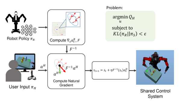
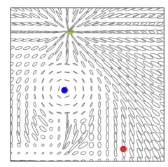
In this work, we formulate shared control as an optimization problem, as shown in Figure 1. The shared control action is chosen to maximize the user’s internal action-value function while we constrain the shared control policy not to diverge away from the autonomous robot policy. We construct the Fisher information matrix which expresses how sensitive a distribution changes in the local neighborhood of the state. When the robot policy is represented as a vector field over the state space, the user can maintain more control authority in regions where the field does not diverge. On the contrary, the inverse Fisher information matrix adjusts the user’s actions so that the robot gains more authority where the robot policy is rapidly changing in the local region (e.g. near an obstacle or near a goal). Utilizing the Fisher information matrix we introduce the term “Natural gradient shared control”.

To assess the efficacy of the approach, we define a teleoperation task where a user performs pick-and-place tasks with a simulated robot arm and compare the quantitative metrics. We show that our shared control paradigm can assist the user towards accomplishing the goal while enabling more control authority to the user.

We summarize our main contributions as the following:

• A shared control paradigm that relies on natural gradients emerging from the divergence constraint between the robot and the shared policy

• Estimating the Fisher information matrix by sampling the autonomous robot policy and computing the local gradient using the finite difference method

• Generating an autonomous robot policy that only relies on task space states and can be regressed over the entire state space

• Quantitative results of a preliminary human user study including 16 participants that shows the potency of the proposed paradigm to allow more control authority to the user

This paper is structured as follows: we present relevant related work in Section II. We review the background theory that underlies our concept of using natural gradients in Section III. Sections IV and V introduce our framework and explain the implementation. The overview of our pilot user study method is described in Section VI and we present the results in Section VII. Finally conclusions are drawn in Section VIII.

II RELATED WORK

II-A Shared Control

Shared control refers to a cooperation between the user and the autonomous robot agent to achieve a common task at a control level [9]. In previous works, different paradigms for shared control have been developed depending on the task and purpose of the application. We categorize the paradigms in three groups depending on how the agents share control: control switching, direct blending, and indirect blending.

Control switching We refer to control switching as allocating all-or-none assistance during control. It is a discrete switching between full autonomy and direct control depending on a predefined circumstance. Control switching can be momentary: at each state the robot evaluates whether to take over depending on the confidence of the user’s intentions [1] (aggressive mode); or to prevent the system from entering an unsafe state [7]. Control switching is also referred to as Traded control when the robot takes over and autonomously executes a sub-task over a sequence of timesteps [10, 11, 12].

Direct blending It involves explicitly combining both agents’ control using an arbitration function. The above control switching corresponds to when the step function is used as the arbitration function. Approaches include using a linear function [1, 3, 4], a sigmoid function [13], specifically tuned [14, 15], or learned [2, 16]. It can be tedious to define and tune an arbitration function that generalizes between users and tasks. As a result, the blended action may be worse than following one of either policy.

Indirect blending We relate to Indirect blending when the shared control is a result of an optimization problem. Javdani et al. [6] formulated the problem as a POMDP and approximated using hindsight optimization to provide assistance which minimizes the expected cost-to-go for an unknown goal. Reddy et al. [17] used deep Q-learning to select an action closest to the user’s suggestion while being suboptimal in discrete states. Broad et al. [8] introduced shared control with “minimal intervention”, such that the human’s command is perturbed when the system leads to an inevitable collision state. Similarly, our work does not directly blend the controls despite the presence of the autonomous robot action but rather computes a metric based on the topology of the autonomous policy in the local neighborhood and adjusts the user commands.

II-B Natural Gradients

The natural gradient adjusts the direction of the standard gradient according to the underlying Riemannian structure of the parameter space. It is effective when the direction of the standard gradient descent does not represent the steepest descent direction of the cost function in the parameter space which lead to poor convergence [18, 19].

The natural gradient is advantageous as it is invariant under coordinate transformations and unlike Newton’s method, it doesn’t assume the cost function as locally-quadratic. It is widely applicable to non-linear functions in neural networks [18], including reinforcement learning methods such as policy gradient [20] and actor-critic [21]. In Schulman et. al [22], a trust-region is defined by constraining the KL-divergence between the old and the new policy during policy updates. Similarly, our shared control framework imposes a constraint on the KL-divergence of the autonomous policy and the shared control policy such that the shared control policy does not diverge far from the autonomous robot policy.

III Understanding Natural Gradients

Gradient descent is a procedure to locally minimize a function $f(\theta)$ by updating its parameters. It can be written as an optimization problem where we minimize a linear approximation of the function $f(\theta)$ subject to the constraint that the distance in the step $\delta\theta=\theta-\theta_{t}$ is marginal [23]: θf(θ_t)+∇f(θ_t)^T(θ-θ_t) ——θ-θ_t——^2_G = ϵ^2 The natural gradient descent computes the distance over the manifold in the Riemannian space that the coordinates parameterize. It is measured as $|\delta\theta|^{2}\equiv\sum_{ij}G_{ij}(\theta)\delta\theta_{i}\delta\theta_{j}=\delta\mathbf{\theta}^{T}G(\theta)\delta\mathbf{\theta}$ (in vector notation) where $G(\theta)$ is called the Riemannian metric tensor which characterizes the intrinsic curvature of a particular manifold in $N$-dimensional space. The natural gradient is then defined as

$$\tilde{\nabla}f=F^{-1}\nabla f$$ (1)

It is equivalent to standard gradient descent when $G(\theta)$ is the identity matrix, such that $|\delta\theta|^{2}$ is equivalent to the squared Euclidean norm [18]. When $G(\theta)$ is a positive-definite Hessian, it corresponds to taking Newton direction steps in the Newton’s method. However, Newton’s method and natural gradient adaptation differ in general: $G(\theta)$ is always positive-definite by construction and the Hessian may not be [19]. When $G(\theta)$ lies in the parameter space of a statistical model, $G(\theta)$ refers to the Fisher information matrix $F(\theta)$.

The Fisher information $F(\theta)$, by definition, measures the expectation of the overall sensitivity of a probability distribution $p(x|\theta)$ to changes of $\theta$. It is defined as the variance of the $\textit{score}=\frac{d}{d\theta}\log p(x|\theta)$, which indicates the sensitivity of the model to changes in $\theta$ [24].

$$F(\theta) =\mathop{\mathbb{E}}_{p(x|\theta)}\Big{[}\Big{(}\frac{d}{d\theta}\log p(x|\theta)\Big{)}^{2}\Big{]}$$ (2)

$$=-\int p(x|\theta)\frac{d^{2}}{d\theta^{2}}\log p(x|\theta)dx$$

Most importantly to our interest, the Fisher information is the second order derivative of the KL-divergence [23][25].

$$F(\theta) =-\int p(x|\theta)\nabla^{2}_{\theta^{\prime}}\log p(x|\theta^{\prime})\big{|}_{\theta^{\prime}=\theta}dx$$ (3)

$$=H_{\mathrm{KL}(p(x|\theta||p(x|\theta^{\prime})))}$$

This gives the key to the connection between natural gradient and the KL-divergence, where KL-divergence is the function to measure the “distance” in gradient descent [26] as below:

$$\mathrm{KL}(p(x|\theta)||p(x|\theta^{\prime}))\approx\frac{1}{2}\delta\theta^{T}F(\theta)\delta\theta$$ (4)

We use Equations 2-4 in the following section to solve our optimization problem and approximate the Fisher information matrix.

IV Natural Gradient Shared Control

IV-A Expressing Shared Control as an Optimization Problem

Let $s\in\mathcal{S}$ be the state of the system. Let $a^{H}\in\mathcal{A^{H}}$ as the user action, $a^{R}\in\mathcal{A^{R}}$ be the autonomous robot action, and $u\in\mathcal{U}$ be the shared control action. The human and the robot agent each select actions following their stochastic policies, $\pi_{H}$, and $\pi_{R}$. Our goal is to find a shared control policy $\pi_{S}$ that solves the following optimization problem. u_tQ_H (s_t, u_t) KL(π_R ∥ π_S) ¡ ϵ

The shared control policy is chosen to maximize the user’s internal action-value function $Q_{H}(s_{t},u_{t})$ at each step. Although it is possible to learn $Q_{H}$ using methods such as MaxEnt IOC [27], predicting the user controls $a^{H}_{t}$ can be challenging due to interpersonal differences. Instead, we regard the user action as an estimate of $\nabla_{s}Q_{H}(s_{t},a^{H}_{t})$ at each step.

The constraint on the KL-divergence between the robot policy and the shared policy ensures that the shared policy does not deviate far from the autonomous robot policy. The problem can be expressed using a Lagrange Multiplier, assuming a linear approximation of our objective $\nabla_{s}Q_{H}(s_{t},a^{H}_{t})$ and a quadratic approximation of the KL-divergence constraint. Solving this approximation of the Lagrangian leads to an update rule which introduces natural gradient adaptation.

for $t=1,T$ do

      Observe user action $a^{H}_{t}$

      foreach $g\in\mathcal{G}$ do

           Compute belief $b_{t,g}$

           $F_{g}(s_{t})=$ ComputeFisher($s_{t},g$)

          

           end foreach

          $F(s_{t})^{-1}=\sum_{g}b_{t,g}F_{t,g}^{-1}(s_{t})$

            $\triangleright$ weighted sum over goals

           $u_{t}\leftarrow F(s_{t})^{-1}a^{H}_{t}$

            $\triangleright$ compute shared action

           $s\leftarrow s+\eta u_{t}$

            $\triangleright$ update state

          

           end for

Algorithm 1 Natural Gradient Shared Control

IV-B Natural Gradient Shared Control

We introduce a new control paradigm for shared control using natural gradient adaptation. Note that our goal is to find the action that maximizes $Q_{H}$, resulting in taking gradient steps in the direction of ascent.

$$s_{t+1} =s_{t}+\eta F(s_{t})^{-1}\nabla_{s}Q_{H}(s_{t},a^{H}_{t})$$ (5)

$$=s_{t}+\eta u_{t}$$

$\eta$ is the step size and the natural gradient in Equation 1 corresponds to the shared control action ${u_{t}\sim\pi_{S}(\cdot|s_{t},a^{H}_{t},a^{R}_{t})}$. We utilize the approximation ${a^{H}_{t}\propto\nabla_{s}Q_{H}(s_{t},a^{H}_{t})}$ in Equation 7. The proportionality constant is absorbed by the step size $\eta$. The overall algorithm is summarized in Algorithm 1.

$$u_{t} =F(s_{t})^{-1}\nabla_{s}Q_{H}(s_{t},a^{H}_{t})$$ (6)

$$=F(s_{t})^{-1}a^{H}_{t}$$ (7)

The Fisher information matrix $F(s_{t})$ can be interpreted as the sensitivity of the autonomous robot policy $\pi_{R}$ to changes of the parameter.

Intuitively, a deterministic robot policy regressed over the whole state space defines a vector field. This vector field integrates information about which optimality and constraint trade-offs are made about the underlying actions. For example when an obstacle is in an environment, it acts as a source (positive divergence) in the vector field resulting in a repulsive action. When the policy is goal-directed, the goal acts as a sink (negative divergence). The vectors around the goal point inward. $F$ measures how sensitive the field changes and emphasizes or discounts towards certain directions of $u_{t}$.

Init: Load pre-trained robot policy model $f_{nn}$

Input: $s_{t},g$

Output: $F_{t,g}$

Function ComputeFisher($s_{t},g$):

      Sample set of states $\mathcal{S}=\{(s_{i},g)\}^{N}_{i=1}$

      Infer robot actions $\mathcal{D}=f_{nn}(\mathcal{S})$

      Fit LWR model $L_{g}=\textrm{LWR}(\mathcal{S},\mathcal{D})$

      $\tilde{a}^{R}_{t,g}\leftarrow L_{g}(s_{t})$

       $\triangleright$ query action from LWR

      $H_{t,g}\leftarrow\nabla_{s}\tilde{a}^{R}_{t,g}$

       $\triangleright$ compute Jacobian of action

      $F_{t,g}\leftarrow\frac{1}{2}(H_{t,g}+H_{t,g}^{T})$

       $\triangleright$ ensure symmetry

      return $F_{t,g}$

     

     

     End Function

Algorithm 2 Computing Fisher Information Matrix

IV-C Computing the Fisher Information Matrix

We approximate $F$ as the curvature of the robot’s action-value function at a given state:

$$F(s_{t}) =\displaystyle\mathop{\mathbb{E}}_{\pi_{H}}[\nabla_{s}\log\pi_{R}(a^{R}_{t}|s_{t})\nabla_{s}\log\pi_{R}(a^{R}_{t}|s_{t})^{T}]$$ (8)

$$\approx\nabla_{s}^{2}Q_{R}(s_{t},a_{t})$$ (9)

Keeping in mind the connection between $F$ and the KL-divergence and the asymmetry of the KL-divergence, one may ask how dependent is $F$ to the underlying assumption of $\mathrm{KL}(p||q)$ or $\mathrm{KL}(q||p)$. It turns out that when $p$ and $q$ are close, the KL-divergence is locally/asymptotically symmetric [26]. Hence our definition for $F\approx\nabla_{s}^{2}Q_{R}$ is equivalent to integrating the user actions over all possible robot actions.

We describe our method for computing $F$ in Algorithm 2, where $F$ is computed at each state for each goal. We use Locally Weighted Regression (LWR) to fit a local model $L_{g}$ using a set of sampled states and actions inferred using a pre-trained model. A detailed explanation regarding LWR is described in Subsection V-B. As we consider action as an approximate of the first derivative of the Q-function, we consider the Jacobian of the robot action w.r.t. state $\nabla_{s}a^{R}_{t}$ as the Hessian of the Q-function. $\nabla_{s}\tilde{a}^{R}_{t}$ is the Jacobian computed using the finite difference method with actions $\tilde{a}^{R}_{t,g}$ from $L_{g}$. The Fisher information matrix $F$ is positive-definite by definition. However, the Jacobian computed using the finite difference method may not always be symmetric. Thus, We decompose the matrix as a sum of symmetric and a skew-symmetric matrix and apply the symmetric matrix.

(a) Single goal

(b) Belief-weighted
over goals

(c) Obstacle avoidance

Figure 2: Ellipse plots from the eigenvalues, eigenvectors of $F(s)^{-1}$ for (a) a single goal and (b) in the presence of multiple goals computed as weighted sum over beliefs, (c) obstacle avoidance

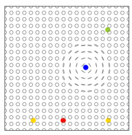
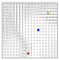
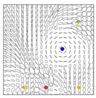
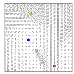
The objective of the robot assistance can be flexibly defined depending on the cost function that the robot policy optimizes. Figure 2 shows the $F(s)^{-1}$ computed over the state space with different assistance modes; the robot assistance can be goal-directed (in Figure 2(a)) or it can minimally assist to avoid obstacles (in Figure 2(c)). The ellipse represents the direction that the user’s action is stretched along. When the ellipse is close to a circle the user has more control authority over the system. When the ellipse is narrow, for example near an obstacle, the robot augments the user’s action towards one direction.

In the case of goal-directed assistance with multiple goals, the robot must predict a goal among goal candidates. We compute $F(s_{t})^{-1}$ as a weighted sum over the beliefs which represent the confidence of the goal prediction. Figure 2(b) shows $F(s_{t})^{-1}$ computed using beliefs as a naive distance-based goal prediction. It is shown that when the confidence is low (right top corner, or above the left two objects), user gains more control authority.

V Autonomous Robot Policy Generation

V-A Learning a Robot Policy

We train a neural network policy that imitates optimized robot trajectories. Given the system’s state $s_{t}$ and a goal $g$, the network infers a normalized velocity $v_{gripper}$ and end-effector rotation $\mathbf{v}_{rot_{Z}}$ that represents an optimal action towards the goal. The network is regressed over the whole state space, such that it can infer an optimal action at any state that the robot is located in. This is advantageous when the robot state is modified with user inputs.

The overview of the training network is shown in Figure 3. The state $\tilde{s}_{t}$ is a concatenation of robot and environment states consisting of: end-effector position $p_{gripper}$, vector components of current gripper rotation in z-axis

$$\mathbf{v}_{rot_{Z}}=[\cos\varphi,\sin\varphi]^{T}$$ (10)

obstacle position $p_{obstacle}$, as well as the position $p_{goal}$ of the inferred goal. In the pick phase $p_{goal}$ refers to the position of the predicted goal object and in the place phase $p_{goal}$ refers to where the object should be placed. In our experiment, we constrict our environment to a 2-dim plane over the workspace.

The state and action space of our robot policy are solely defined in task space. Consequently, the network must learn to distinctively output end-effector actions such that it avoids collision when joint configurations are computed using inverse kinematics. We collect training data by computing pick-and-place trajectories with random starting positions and environment configurations using a Gauss-Newton trajectory optimizer [28] that is tuned to perform specific pick-and-place motions.

Figure 3: Overview of the training network. We use supervised learning to mimic optimal trajectory actions $a^{R}_{t}$ while using a multi-loss to infer additional features such as $p_{approach}$ and $V(s)$

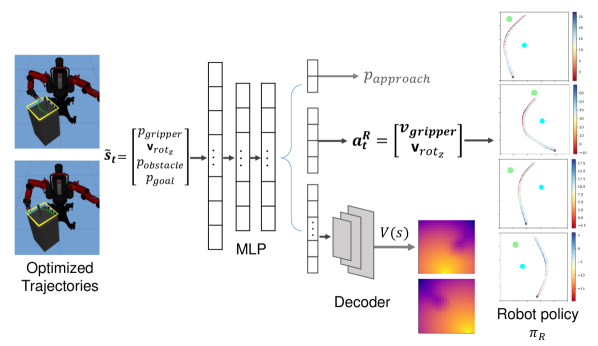
To improve training, we use a multi-loss function to penalize/enforce specific behaviors. In the pick phase, we add an additional cost term to predict the approach position $p_{approach}$, which is a data point in the optimal trajectory that the gripper reaches when approaching the object. This ensures that the gripper approaches the object in the direction parallel to the gripper fingers for grasping.

In addition, we learn a feature-based cost function of the environment and compute the state log partition function $V(s)$ using MaxEnt IOC [27, 29]. The state log partition function $V(s)$ is a soft estimate of the expected cost to reach the goal from a state $s$. Here, even though we limit the state/action space to 2-dim position and discrete neighboring actions, we were able to generate smoother trajectories by enforcing the network to reconstruct the learned $V(s)$ (shown as heatmaps in Figure 1) from the latent layer of the network using a series of convolutions and up-sampling layers.

(a) Pick policy

(b) Place policy

Figure 4: First row: Vector field of the robot policy (green arrows) and the LWR fit policy (red arrows) projected onto position space. Second row: Ellipse plots from the eigenvalues and eigenvectors of $F(s)^{-1}$. Red, blue, green dots each correspond to positions of the object, obstacle, and goal.

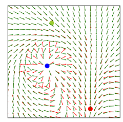
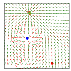
The robot policy is represented as a vector field over the state space, as shown in green arrows in the top row of Figure 4. It shows positive divergence from the obstacle and negative divergence towards a goal. When strictly following the inferred action at each state, the robot generates an autonomous pick-and-place trajectory with a success rate of 95% in random environments.

V-B Fitting Locally Weighted Regression Models

Locally Weighted Regression (LWR) fits a regression model that is valid only in the local region given a set of data points around the point of interest [30]. Since the resulting model is linear, we fit the robot policy to a LWR model to reduce any non-linearity generated by the output of the network. The model is used to query data points to compute smoother Jacobians using the finite difference method, as part of the process to compute $F$ described in Subsection IV-C.

Another advantage of using LWR is that we can augment the model by providing additional data points since the model is fit only in the local region. This is useful to improve the behavior of the learned policy. For instance, we prefer the learned policy to enforce stronger obstacle avoidance, thus we provide additional data points computed using a signed distance field when fitting LWR near the obstacle.

The vector fields of the policies regressed using LWR are shown as red arrows in the top row in Figure 4. The LWR model successfully approximates the neural network policy, as well as augmenting a stronger repulsion in neighboring points of the obstacle.

VI EXPERIMENTS

VI-A Experimental System

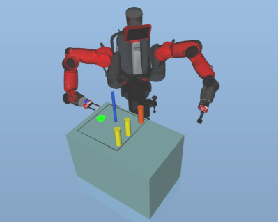
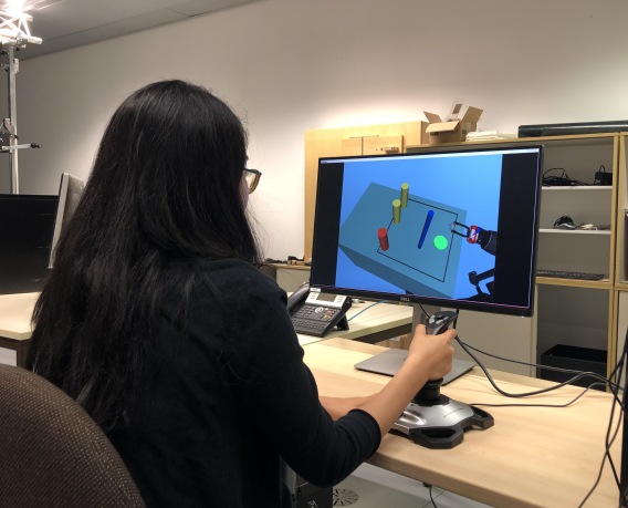
We perform a human participant study to assess the efficacy of our method. We define a simulated teleoperation environment, which consists of the Baxter robot that operates in a $50\text{cm}\times 50\text{cm}$ workspace over a table (see Figure 5) and multiple cylinders that represent objects and an obstacle. The user controls the robot’s right arm end-effector using a joystick (Logitech Extreme 3D Pro). The robot is controlled at around 30Hz. Physical collisions are not simulated in the environment and grasping is simulated by attaching the object to the gripper when grasping is initiated. We hypothesize the following:

• The natural gradient shared control method allows the user to take more control during the task while ensuring safety and efficiency.

Figure 5: Teleoperation workspace setup (left) and user interaction using a joystick (right)

VI-B User Study Procedure

The user study comprised of 16 participants (12 male, 4 female) with the right hand all being their dominant hand. The participants had no noticeable prior experience with robots and gave their informed consent before starting the study.

Users were asked to teleoperate the robot’s gripper using the joystick to pick the red cylinder and bring it back to the green goal position while avoiding the blue pole as shown in Figure 5. The users controlled the robot’s arm in task space: the gripper’s velocity using pitch and roll motions and the z-axis rotation using the yaw motion of the joystick. Grasping was initiated using the trigger button. Users were provided with a perspective view of the robot’s workspace (see Figure 5 right) to simulate a teleoperation scenario with limited camera view.

We chose a within-subjects design, where each user participated in all systems. Each user performed three sets of demonstrations. Each set consisted of four different environments repeated over the control methods: in total 16 of episodes. The random order of teleoperation was predefined and balanced over the study. The teleoperation methods were as following:

• DC: Direct Control

• NG: Natural Gradient Shared Control

• LB: Linear Blending

• OA: Obstacle Avoidance

For LB, we followed the “timid” mode for linear arbitration suggested in Dragan et.al. [1]. The robot policy described in V-A was also using the robot policy described in. Minimal assistance was provided to avoid the obstacle in OA using a signed distance function as shown in Figure 2(c). In all cases, the speed of the action was determined by the user.

VII RESULTS

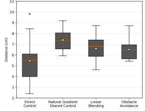
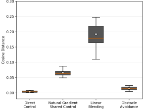
We evaluate the results using a repeated measures analysis of variance (ANOVA), where the assistance method was used as a factor. We compared four quantitative measures as shown in Table I and Figure 6: task duration, travel distance, minimum proximity to the obstacle, and the cosine distance between actions. The results show that our method was effective in assisting while allowing more user control authority.

TABLE I: User study results: Mean and standard deviation

Method	Duration	Travel Dist.	Proximity	Cosine Dist.
	(s)	(cm)	(cm)	($\times$ ${10}^{-2}$)
DC	14.1 $\pm$ 3.5	163.0 $\pm$ 26.2	5.5 $\pm$ 1.8	0.4 $\pm$ 0.25
NG	12.7 $\pm$ 2.8	155.2 $\pm$ 20.5	7.4 $\pm$ 1.0	6.6 $\pm$ 1.0
LB	15.2 $\pm$ 4.0	148.0 $\pm$ 14.6	6.6 $\pm$ 1.1	19.2 $\pm$ 5.2
OA	16.5 $\pm$ 4.2	191.2 $\pm$ 40.4	6.5 $\pm$ 0.9	1.5 $\pm$ 0.6

(a) Duration

(b) Travel distance

(c) Minimum proximity to obstacle

(d) Cosine distance

Figure 6: Comparison of control paradigms across all users for (a) execution time, (b) travel distance, (c) minimum proximity to obstacle, (d) cosine distance.

(a) Direct control

(b) Natural Gradient Shared Control

(c) Linear Blending

(d) Obstacle Avoidance

Figure 7: Top-down visualization of user demonstrations for teloperation method (rows) of three environments (columns).

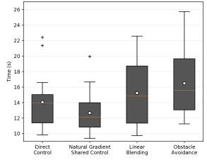
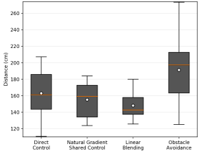
When comparing the average task duration in Figure 6 (a), NG reported the shortest duration over all other methods with statistical significance: DC($f(4,12)=20.67,p=0.0004$), LB($f(4,12)=16.93,p=0.0009$), and LB($f(4,12)=61.50,p<0.0001$). When comparing the travel distance of the end-effector in Figure 6 (b), LB showed the lowest average distance followed by NG. However, the results were statistically equivalent compared to NG ($f(4,12)=1.7933,p=0.2005$). This implies that NG is capable of providing assistance towards achieving efficient teleperation.

We compared the average minimum proximity between the gripper and the obstacle as a notion of safety. The closer distance denotes that it is more likely to collide to the obstacle. As shown in Figure 6 (c), NG showed to provide highest obstacle avoidance compared to all other methods with statistical significance: DC($f(4,12)=31.42,p<0.0000$), LB($f(4,12)=18.7363,p=0.0006$), and OA($f(4,12)=23.2720,p=0.0002$).

The cosine distance represents the amount of disagreement between the user and the executed command. As shown in Figure 6 (d), the average cosine distance of NG is significantly smaller than LB ($f(4,12)=104.36,p<0.0000$) suggesting that the method performed actions closer to what the user intended thus supporting our hypothesis that NG would allocate more control authority. DC and OA naturally showed the lowest in cosine distance since there was zero or minimum assistance.

In LB, assistance is provided such that the robot proceeds towards the optimal path. When the prediction is wrong with high confidence, the user must give an exaggerated opposing command to fight off the autonomous robot actions. This explains the results shown in Figure 6, in which the travel distance was low but still showed large variance in task duration and cosine distance.

Figure 7 shows trajectories of user demonstrations in three environments. As seen from quantitative results, DC and OA trajectories exhibit divergent paths compared to NG or LB methods. Trajectories include dragging along the workspace boundary or approaching the place position from various directions. One notable characteristic of the LB method is shown in the second column of Figure 7. Since the target object and another object were relatively close in this environment, assistance was often provided towards the wrong goal. The user had to fight against the assistance and noisy trajectories are are near the objects.

Overall, NG showed reliable performance in task execution while still maintaining compliance with user commands. The results show that our method can be an option towards reducing the discrepancy and increasing user satisfaction during teleoperation.

VIII CONCLUSIONS

We proposed a formalism for shared control that is based on natural gradients emerging from the divergence constraint between the user and robot policy. We introduced a method to approximate the Fisher information matrix, as a second derivative of the Q-function. The efficacy of the system was demonstrated through a pilot user study and the initial results to quantitative measures showed that our approach allows efficient task completion while allowing more control authority to the user. We believe the results are convincing towards positive user experience and we plan to investigate it in our future work.

References

- [1] A. D. Dragan and S. S. Srinivasa, “A policy-blending formalism for shared control,” The International Journal of Robotics Research, vol. 32, no. 7, pp. 790–805, 2013.
- [2] A. Goil, M. Derry, and B. D. Argall, “Using machine learning to blend human and robot controls for assisted wheelchair navigation,” in 2013 IEEE 13th International Conference on Rehabilitation Robotics (ICORR). IEEE, 2013, pp. 1–6.
- [3] S. J. Anderson, J. M. Walker, and K. Iagnemma, “Experimental performance analysis of a homotopy-based shared autonomy framework,” IEEE Transactions on Human-Machine Systems, vol. 44, no. 2, pp. 190–199, 2014.
- [4] M. Gao, J. Oberländer, et al., “Contextual task-aware shared autonomy for assistive mobile robot teleoperation,” in 2014 IEEE/RSJ International Conference on Intelligent Robots and Systems. IEEE, 2014, pp. 3311–3318.
- [5] D.-J. Kim, R. Hazlett-Knudsen, et al., “How autonomy impacts performance and satisfaction: Results from a study with spinal cord injured subjects using an assistive robot,” IEEE Transactions on Systems, Man, and Cybernetics-Part A: Systems and Humans, vol. 42, no. 1, pp. 2–14, 2011.
- [6] S. Javdani, H. Admoni, et al., “Shared autonomy via hindsight optimization for teleoperation and teaming,” The International Journal of Robotics Research, vol. 37, no. 7, pp. 717–742, 2018.
- [7] A. Broad, T. Murphey, and B. Argall, “Operation and imitation under safety-aware shared control,” in Workshop on the Algorithmic Foundations of Robotics, 2018.
- [8] ——, “Highly parallelized data-driven mpc for minimal intervention shared control,” in Robotics: science and systems, 2019.
- [9] F. Flemisch, D. Abbink, et al., “Shared control is the sharp end of cooperation: Towards a common framework of joint action, shared control and human machine cooperation,” IFAC-PapersOnLine, vol. 49, no. 19, pp. 72–77, 2016.
- [10] J. Kofman, X. Wu, et al., “Teleoperation of a robot manipulator using a vision-based human-robot interface,” IEEE transactions on industrial electronics, vol. 52, no. 5, pp. 1206–1219, 2005.
- [11] C. Smith, M. Bratt, and H. I. Christensen, “Teleoperation for a ball-catching task with significant dynamics,” Neural Networks, vol. 21, no. 4, pp. 604–620, 2008.
- [12] C. Phillips-Grafflin, H. B. Suay, et al., “From autonomy to cooperative traded control of humanoid manipulation tasks with unreliable communication,” Journal of Intelligent & Robotic Systems, vol. 82, no. 3-4, pp. 341–361, 2016.
- [13] K. Muelling, A. Venkatraman, et al., “Autonomy infused teleoperation with application to bci manipulation,” arXiv preprint arXiv:1503.05451, 2015.
- [14] D. Gopinath, S. Jain, and B. D. Argall, “Human-in-the-loop optimization of shared autonomy in assistive robotics,” IEEE Robotics and Automation Letters, vol. 2, no. 1, pp. 247–254, 2016.
- [15] S. Jain and B. Argall, “An approach for online user customization of shared autonomy for intelligent assistive devices,” in Proc. of the IEEE Int. Conf. on Robot. and Autom., Stockholm, Sweden, 2016.
- [16] Y. Oh, M. Toussaint, and J. Mainprice, “Learning arbitration for shared autonomy by hindsight data aggregation,” in Workshop on AI and Its Alternatives for Shared Autonomy in Assistive and Collaborative Robotics, 2019.
- [17] S. Reddy, A. D. Dragan, and S. Levine, “Shared autonomy via deep reinforcement learning,” arXiv preprint arXiv:1802.01744, 2018.
- [18] S.-I. Amari, “Natural gradient works efficiently in learning,” Neural computation, vol. 10, no. 2, pp. 251–276, 1998.
- [19] S.-I. Amari and S. C. Douglas, “Why natural gradient?” in Proceedings of the 1998 IEEE International Conference on Acoustics, Speech and Signal Processing, ICASSP’98 (Cat. No. 98CH36181), vol. 2. IEEE, 1998, pp. 1213–1216.
- [20] S. M. Kakade, “A natural policy gradient,” in Advances in neural information processing systems, 2002, pp. 1531–1538.
- [21] J. Peters and S. Schaal, “Natural actor-critic,” Neurocomputing, vol. 71, no. 7-9, pp. 1180–1190, 2008.
- [22] J. Schulman, S. Levine, et al., “Trust region policy optimization,” in International conference on machine learning, 2015, pp. 1889–1897.
-
[23]
N. Ratliff, “Information geometry and natural gradients,” 2013. [Online].
Available:
https://ipvs.informatik.uni-stuttgart.de/mlr/wp-content/uploads/2015/01/
mathematics_for_intelligent_systems_lecture12_notes_I.pdf - [24] A. Ly, M. Marsman, et al., “A tutorial on fisher information,” Journal of Mathematical Psychology, vol. 80, pp. 40–55, 2017.
- [25] A. Kristiadi. (2018, Mar.) Natural gradient descent. [Online]. Available: https://wiseodd.github.io/techblog/2018/03/14/natural-gradient/
- [26] J. Martens, “New insights and perspectives on the natural gradient method,” arXiv preprint arXiv:1412.1193, 2014.
- [27] B. D. Ziebart, N. Ratliff, et al., “Planning-based prediction for pedestrians,” in 2009 IEEE/RSJ International Conference on Intelligent Robots and Systems. IEEE, 2009, pp. 3931–3936.
- [28] J. Mainprice, N. Ratliff, and S. Schaal, “Warping the workspace geometry with electric potentials for motion optimization of manipulation tasks,” in 2016 IEEE/RSJ International Conference on Intelligent Robots and Systems (IROS). IEEE, 2016, pp. 3156–3163.
- [29] K. M. Kitani, B. D. Ziebart, et al., “Activity forecasting,” in European Conference on Computer Vision. Springer, 2012, pp. 201–214.
- [30] C. G. Atkeson, A. W. Moore, and S. Schaal, “Locally weighted learning,” in Lazy learning. Springer, 1997, pp. 11–73.