Multiple phases in a generalized Gross-Witten-Wadia matrix model

Abstract

We study a unitary matrix model of the Gross-Witten-Wadia type, extended with the addition of characteristic polynomial insertions. The model interpolates between solvable unitary matrix models and is the unitary counterpart of a deformed Cauchy ensemble. Exact formulas for the partition function and Wilson loops are given in terms of Toeplitz determinants and minors and large $N$ results are obtained by using Szegö theorem with a Fisher-Hartwig singularity. In the large $N$ (planar) limit with two scaled couplings, the theory exhibits a surprisingly intricate phase structure in the two-dimensional parameter space.

1 Introduction

The study of random matrix ensembles has been a subject developing for many decades already. The array of applications is vast by now and ever expanding Mehta ; Forrester ; BDS . Among the many aspects of random matrices that can be studied is the analysis of phase transitions in a so-called double scaling limit.

This type of analysis is relevant for example in the study of phase transitions in gauge theories. When combined with localization results, which effectively provide integral representation, of random-matrix type, of observables of the gauge theory, such as partition functions or Wilson loop averages, this analysis is especially potent and has led to many novel results in the study of supersymmetric and topological gauge theories.

In this context, the matrix models are typically and predominantly models of Hermitian random matrices. However, another important type of matrix models are the unitary matrix models, such as Dyson’s circular ensembles Mehta or the matrix model of Gross and Witten Gross:1980he and Wadia Wadia:2012fr ; Wadia:1980cp , for example.

The unitary group $U(N)$ with Haar measure has eigenvalue probability density function (see (Forrester, , Chapter 2), for example)

$$\frac{1}{(2\pi)^{N}N!}\prod_{1\leq j<k\leq N}|z_{k}-z_{j}|^{2},\quad z_{l}:=e^{i\theta_{l}}\in\mathbb{T},\quad\theta_{l}\in(-\pi,\pi],$$ (1)

where $\mathbb{T}=\{z\in\mathbb{C}:|z|=1\}$. By unitary matrix model, we refer to the setting where one studies averages over $U\in U(N)$ of functions $w(U)$, which are symmetric functions of the eigenvalues of $U$ only (class functions) with the factorization property $\prod_{l=1}^{N}w(z_{l})$ for $\{z_{1},\dots,z_{N}\}\in{\rm Spec}(U)$. Writing down the Fourier components $\{w_{l}\}_{l\in\mathbb{Z}}$ of the weight $w(z)=\sum_{l=-\infty}^{\infty}w_{l}z^{l}$, it holds that Forrester

$$\Big{\langle}\prod_{l=1}^{N}w(z_{l})\Big{\rangle}_{U(N)}=\det[w_{i-j}]_{i,j=1,\dots,N},$$ (2)

relating the partition function with the determinant of a Toeplitz matrix, whose entries are the Fourier coefficients of the weight function. We will make use of this equivalent Toeplitz determinant formulation below.

As we shall explain in the next Section, the Gross-Witten-Wadia (GWW) model corresponds to the case where the weight function is:

$$\omega(z)=\exp(t(z+z^{-1})),$$ (3)

where $t$ is a real parameter, although we will be using the original physics notation in Gross:1980he , in terms of a coupling constant.

One of the main aspects associated with this model is that it exhibits a third-order phase transition at large $N$ Gross:1980he ; Wadia:2012fr . The study of this transition has lead to many delicate results and its detailed analysis also encompasses many influential works in mathematics as well, involving also the Tracy-Widom law and culminating in the seminal solution of the long-standing conjecture (as it was proposed by Ulam in the early 1960s) on the longest increasing subsequence of a random permutation, by Baik, Deift and Johansson BDJ ; BDS ; Romik .

On the other hand, models involving other weights, that correspond to a pure Fisher-Hartwig (FH) singularity in the context of Toeplitz matrices Toep-book , such as

$$\omega\left(z\right)=(1+z)^{\alpha}(1+z^{-1})^{\beta}\ ,$$ (4)

are actually solvable even at finite $N$ and have been also thoroughly studied, with many mathematical applications in problems in combinatorics, representation theory and number theory Forrester ; BDS . Here $\alpha$ and $\beta$ are real parameters that will be equal in our discussion below. Both models emerge in the study of probability measures associated to partitions (see TW , for example).

In this work, we shall be studying a unitary matrix model that is made of both terms and we will be stressing its large $N$ behavior and the ensuing phase transitions in scaling limits involving the two parameters present.

2 New unitary matrix model from deformation of GWW model

By an appropriate axial gauge choice, two-dimensional lattice $U(N)$ gauge theory with Wilson lattice action is effectively described by a random unitary matrix model, with partition function

$$Z=\int dUe^{\frac{1}{g^{2}}\mathrm{Tr}(U+U^{\dagger})},$$ (5)

where $g$ is the coupling constant and only parameter in the theory. Integrating over the volume of the $U(N)$ group following a standard procedure, one arrives at

$$Z_{N}=\int_{(0,2\pi]^{N}}\prod_{1\leq j<k\leq N}\left|e^{\mathrm{i}\varphi_{j}}-e^{\mathrm{i}\varphi_{k}}\right|^{2}\prod_{j=1}^{N}\exp\left(\frac{2}{g^{2}}\cos\left(\varphi_{j}\right)\right)\frac{\mathrm{d}\varphi_{j}}{2\pi}.$$ (6)

This is the celebrated Gross-Witten-Wadia matrix model Gross:1980he ; Wadia:2012fr alluded above. It has generated a large amount of interest, spanning now four decades. As mentioned above, chief among the reasons for this interest, is the existence of a large $N$ third order phase transition in a double scaling limit.

In this work, we shall study a generalized version of the model, emphasizing the analysis of its phase structure in a number of scaling limits. To obtain our model, we start with the Hermitian matrix model introduced in Russo:2020pnv , with potential

$$V(M)=A\,{\rm Tr}\ln(1+M^{2})+B\,{\rm Tr}\frac{1}{1+M^{2}}\ .$$ (7)

The partition function is given by

$$Z=\frac{1}{N!}\int\frac{d^{N}a}{(2\pi)^{N}}\,\prod_{i<j}^{N}(a_{i}-a_{j})^{2}\,\prod_{i=1}^{N}\frac{\exp[-B/(1+a_{i}^{2})]}{(1+a_{i}^{2})^{A}}\ .$$ (8)

We pass from angular variables to the real line using the usual one-dimensional stereographic projection:

$$e^{\mathrm{i}\varphi}=\frac{1+\mathrm{i}x}{1-\mathrm{i}x},\qquad-\pi<\varphi<\pi,\ x\in{\mathbb{R}}.$$

Thus, we have the following unitary matrix model:

$$Z_{N}=\frac{e^{-\frac{1}{2}BN}}{N!}\int_{(0,2\pi]^{N}}\prod_{1\leq j<k\leq N}\left|e^{\mathrm{i}\varphi_{j}}-e^{\mathrm{i}\varphi_{k}}\right|^{2}\prod_{j=1}^{N}\cos^{2\nu}\left(\frac{\varphi_{j}}{2}\right)\exp\left(-\frac{1}{2}B\cos\left(\varphi_{j}\right)\right)\frac{\mathrm{d}\varphi_{j}}{2\pi}\ .$$ (9)

with $\nu\equiv A-N$. The shift $A\to A-N$ takes into account the Jacobian of the transformation from $a_{j}$ to $\varphi_{j}$ (see WitteForr for the similar calculation in the Cauchy ensemble). As explained in the introduction, this matrix model interpolates between two matrix models. On one hand, for $\nu=0$, it is the celebrated and influential Gross-Witten-Wadia model and, on the other hand, for $B=0$ is the exactly solvable matrix model (4), which is actually very central in random matrix theory Forrester and in the theory of Toeplitz banded matrices Toep-book . Indeed, for $B=0$ the matrix model is

$$\frac{1}{2^{2N\nu}}\Big{\langle}\prod_{l=1}^{N}\left|1+z_{l}\right|^{2\nu}\Big{\rangle}_{U(N)}\ ,$$ (10)

which is the average of a characteristic polynomial over the Circular Unitary Ensemble (CUE) (1) WitteForr ; Forrester and is also a particular case of the pure FH weight (4), when $\alpha=\beta=\nu$. From the point of view of the right hand side of (2), that is, as a Toeplitz determinant, it corresponds to the pure Fisher-Hartwig singularity case, and its exact evaluation is known FH ; Toep-book :

$$\mathcal{Z}_{N}(B=0)=\frac{G(N+1)}{2^{2\nu N}}\frac{G(\nu+1)^{2}G(2\nu+N+1)}{G(2\nu+1)G(\nu+N+1)^{2}}\ ,$$ (11)

where $G(\cdot)$ is the Barnes $G$-function, which, for integer values of the argument is $G(n)=\prod_{j=0}^{n-2}j!$. This result holds for complex $\nu$ with $\Re\left(\nu\right)>-\frac{1}{2}$ FH .

In these two limits, the matrix model partition function is a tau function of Painlevé III’, in the GWW case, or a tau function of Painlevé V for a generalization of (10) Forrester . Among many other aspects, the connection with Painlevé is useful for resurgence computations Ahmed:2017lhl ; Ahmed:2018gbt .

2.1 Finite $N$ partition function and Wilson loops

We can adopt the Toeplitz determinant point of view (2) for finite $N$ evaluations of the partition function. Let us consider the case when $\nu$ is a positive integer. The relationship between our matrix model and the ordinary GWW matrix model is not that of a parametric derivative with regards to $B$. However, the weight function $\omega\left(\varphi\right)$ of our matrix model has this property, as it satisfies

$$\omega\left(\varphi\right)=\frac{1}{2^{\nu}}\left(1+\cos\left(\varphi\right)\right)^{\nu}e^{-\frac{1}{2}B(1+\cos\left(\varphi\right))}=(-1)^{\nu}\frac{d^{\nu}\omega_{\nu=0}(\varphi)}{dB^{\nu}},$$ (12)

for positive integer $\nu.$ It has the well-known expansion

$$\omega_{\nu=0}\left(\varphi\right)=e^{-B/2}\sum_{n\in\mathbb{Z}}(-1)^{n}\ I_{n}(B/2)e^{in\varphi},$$ (13)

where $I_{n}(B)$ are the modified Bessel functions of first kind. The derivative of these Bessel functions can be written as a recurrence relation:

$$\frac{dI_{0}(x)}{dx} = I_{1}(x),$$ (14)

$$\frac{dI_{n}(x)}{dx} = \frac{1}{2}(I_{n-1}(x)+I_{n+1}(x)).$$ (15)

Although the prefactor $e^{-NB/2}$ in (9) is not essential for the definition of the model, as one may define the matrix model without this prefactor, we can take into account by considering derivatives of $e^{-B/2}I_{n}(B/2)$, not just the derivative of the Bessel function, otherwise we would be generating the term $\cos\theta$ in the matrix model, instead of $\cos\left(\theta/2\right)$. One can use the formula

$$\frac{d^{\nu}(e^{-x}I_{n}(x))}{dx^{\nu}}=\sum\limits_{k=0}^{\nu}(-1)^{\nu-k}\binom{\nu}{k}e^{-x}\frac{d^{k}\left(I_{n}(x)\right)}{dx^{k}}\ .$$ (16)

The $kth$ derivative of the Bessel function admits several interesting expressions, including hypergeometric ones. The simplest one is:

$$\frac{d^{k}\left(I_{n}(x)\right)}{dx^{k}}=2^{-k}\sum\limits_{j=0}^{k}\binom{k}{j}I_{2j-k+n}(x).$$ (17)

We have then that (9) is the determinant:

$$Z_{N}(\nu,B)=\frac{1}{2^{\nu N}}\det[w_{i-j}]_{i,j=1,\dots,N},$$ (18)

with

$$w_{i-j}=(-1)^{i-j}\sum\limits_{k=0}^{\nu}\sum\limits_{l=0}^{k}2^{-k}\binom{\nu}{k}\binom{k}{l}e^{-\frac{B}{2}}I_{2l-k+i-j}(\frac{B}{2}).$$ (19)

As for particular cases, we see that $\nu=0$ corresponds indeed to GWW model with the prefactor $e^{-BN/2}$ and, for $\nu=1$, we have that the matrix entry $(i,j)$ is:

$$(-1)^{i-j}e^{-\frac{B}{2}}\left(I_{i-j}(\frac{B}{2})+2^{-1}I_{i-j-1}(\frac{B}{2})+2^{-1}I_{i-j+1}(\frac{B}{2})\right),$$ (20)

in consistency with (15). Notice that there is no problem if $\nu>n$ because it holds that $I_{-\alpha}(\frac{B}{2})=I_{\alpha}(\frac{B}{2}).$ Expressions for higher values of $\nu$ and specific values of $N$ can be quickly generated, case-by-case (as happens with the GWW model) with (19).

We note that the same result can be obtained, without having to consider any derivative of Bessel functions, by carrying out the product of the term $\left(1+\cos\left(\varphi\right)\right)^{\nu}$, which is a polynomial in the variables $e^{i\varphi}$ and $e^{-i\varphi}$, with (13), and then identifying again all the coefficients corresponding to a given power of $z=e^{i\varphi}$. By using the trinomial theorem (or twice the binomial theorem), it is immediate that:

$$\left(1+\cos\left(\varphi\right)\right)^{\nu}=\sum_{k=0}^{\nu}\sum_{l=0}^{k}\frac{1}{2^{k}}\binom{\nu}{k}\binom{k}{l}z^{2l-k},$$ (21)

where $z=e^{i\varphi}$. The product of this expansion with the Bessel expansion of the remaining term, Eq. (13) above, leads then again to (19).

The determinant representation can be applied directly to the study of averages of product of two traces, in arbitrary representations $\tilde{r}$ and $r$:

$$\left\langle W_{N}^{r,\tilde{r}}\right\rangle=\left\langle\mathrm{Tr}_{r}(U)\mathrm{Tr}_{\tilde{r}}(U^{{\dagger}})\right\rangle=\frac{1}{Z_{N}\left(B,\nu\right)}\int dU\omega(U)s_{r}(U)s_{\tilde{r}}(U^{{\dagger}}).$$ (22)

This describes, when we only have one trace (taking the void partition, $\tilde{r}=\varnothing$, for example), Wilson loops in arbitrary representation. The determinant description is now:

$$\left\langle W_{N}^{r,\tilde{r}}\right\rangle=\frac{\det[w_{i-\tilde{r}_{i}-j+r_{j}}]_{i,j=1,\dots,N}}{\det[w_{i-j}]_{i,j=1,\dots,N}}.$$ (23)

Hence, the un-normalized average is a minor of the matrix in (18). The striking pattern of columns and rows is described in Minors , but can be read off from (23) as well.

Additionally, there is an extension of Szegö theorem, applicable to these averages Minors . As with the partition function, the result is expressed in terms of the Fourier coefficients of the potential. We summarize a few cases for the model at hand in the Table 1.

boxsize=0.2cm

$\tilde{r}$	$r$	$\lim_{N\rightarrow\infty}\left\langle W_{N}^{r,\tilde{r}}\right\rangle$	$\tilde{r}$	$r$	$\lim_{N\rightarrow\infty}\left\langle W_{N}^{r,\tilde{r}}\right\rangle$
$\varnothing$	$\ydiagram{1}$	$\nu-\frac{B}{4}$	$\varnothing$	$\ydiagram{2}$	$\frac{1}{2}(\nu-\frac{B}{4})^{2}-\frac{\nu}{2}$
$\varnothing$	$\ydiagram{1,1}$	$\frac{1}{2}(\nu-\frac{B}{4})^{2}+\frac{\nu}{2}$	$\varnothing$	$\ydiagram{3}$	$\frac{1}{6}(\nu-\frac{B}{4})^{3}-(\nu-\frac{B}{4})\frac{\nu}{2}+\frac{\nu}{3}$
$\varnothing$	$\ydiagram{1,1,1}$	$\frac{1}{6}(\nu-\frac{B}{4})^{3}+(\nu-\frac{B}{4})\frac{\nu}{2}+\frac{\nu}{3}$	$\varnothing$	$\ydiagram{2,2}$	$\frac{1}{12}(\nu-\frac{B}{4})^{4}-(\nu-\frac{B}{4})\frac{\nu}{3}+\frac{\nu^{2}}{4}$
$\tilde{r}$	$r$	$\lim_{N\rightarrow\infty}\left\langle W_{N}^{r,\tilde{r}}\right\rangle$
$\ydiagram{1,1}$	$\ydiagram{1,1}$	$\frac{1}{4}(\nu-\frac{B}{4})^{4}+(\nu-\frac{B}{4})^{2}+\frac{\nu}{2}(\nu-\frac{B}{4})^{2}+\frac{\nu^{2}}{4}+1$
$\ydiagram{1}$	$\ydiagram{3}$	$\frac{1}{6}(\nu-\frac{B}{4})^{4}+\frac{1}{2}(\nu-\frac{B}{4})^{2}-\frac{\nu}{2}(\nu-\frac{B}{4})^{2}-\frac{\nu}{2}+\frac{\nu}{3}(\nu-\frac{B}{4})$

Table 1: Some large $N$ limit evaluations of Wilson loops.

Expressions for a generic model can be found in Minors , reproduced here for the present model. Two observations then follow:

1. For Wilson loops, they only depend on the positive Fourier coefficients of the potential. Hence, the model with an insertion $(\det(1+U))^{\nu}$ will give the same result as in our model, where the insertion is $(\det(1+U)\det(1+U^{{\dagger}}))^{\nu}$.

2. For the more general case of two traces, they depend on both sets of coefficients, but still the result in the Table is simplified (with regards to the general one in Minors ) due to the symmetry $V(z)=V(z^{-1})$ of our model.

2.2 Large $N$ limits

In section 3 we will be studying the large $N$ limit with fixed ’t Hooft couplings, where $A$ and $B$ scale to infinity like $N$. That is, a triple scaling limit. However, it is interesting to also study large $N$ limits with different scalings. We will now consider two cases: a) no scaling of the couplings and b) the double-scaling limit of the GWW model, where $\nu$ will be finite.

With this aim, we take into account the equivalent Toeplitz determinant description given by (2). The strong Szegö theorem establishes that, in the large $N$ limit, the determinant is, as we have already seen, governed by the Fourier coefficients of the potential.

The large $N$ limit without scaling of couplings ($\nu,B$ fixed)

The $\nu$-dependent term adds a zero to the GWW weight function, and hence we have to consider the Fisher-Hartwig extension of Szegö asymptotics, which for the GWW model gives

$$\lim_{N\rightarrow\infty}Z_{N}(\nu=0)=e^{\frac{B^{2}}{16}-\frac{BN}{2}}.$$ (24)

This is the large $N$ behavior of the GWW without scaling. In the usual double-scaling behavior of the model, this corresponds to the weak-coupling phase.

The asymptotics of the full model is that of the GWW but with a single FH singularity. Note that the FH singularity is just a zero of the weight function $\omega\left(\varphi\right)$ of the model for $\varphi=\pi$. Using the extended formula DAK2 , we obtain:

$$\lim_{N\rightarrow\infty}Z_{N}(\nu,B)=\frac{e^{\frac{B^{2}}{16}-\frac{BN}{2}-\frac{\nu B}{2}}N^{\nu^{2}}G^{2}(1+\nu)}{2^{2N\nu}G(1+2\nu)}.$$ (25)

The term that mixes the two parts of weight function is obviously (and simply) $\exp(-\frac{\nu B}{2})$. The term $N^{\nu^{2}}G^{2}(1+\nu)/G(1+2\nu)$ is the large $N$ limit of the finite $N$ result for the pure FH singularity (11).

Large $N$ limit with fixed $\nu$ and fixed $B/N$

It is convenient to introduce a coupling $g^{2}$ as $B=-4/g^{2}$, to match Gross-Witten notation. We will also omit the multiplicative constant $e^{-NB/2}$ in (9). We would now like to investigate the theory in the large $N$ limit with fixed $\nu=A-N$ and fixed $\lambda\equiv g^{2}N$.

We can study this limit by computing the average of the term $\left[\cos(\theta/2)\right]^{2\nu}$ in the two phases of the GWW matrix model, described by the density of states of the model Gross:1980he , and also given below. Expressing the power of the cosine in terms of a sum of multiple-angle cosines:

$$\cos^{2\nu}\Big{(}\frac{\theta}{2}\Big{)}=\frac{1}{2^{2\nu}}\binom{2\nu}{\nu}+\frac{2}{2^{2\nu}}\sum_{k=0}^{\nu-1}\binom{2\nu}{k}\cos\left(\left(\nu-k\right)\theta\right),$$ (26)

we can then use a non-trivial but well-known result available for averages with $\rho(\phi)$ in the GWW model, Gross:1980he ; Rossi:1996hs ; Okuyama:2017pil ; Alfinito:2017hsh :

$$W_{k} = \int_{-\phi_{c}}^{\phi_{c}}\mathrm{d}\phi\cos k\phi\,\rho(\phi)$$ (29)

$$= \left\{\begin{array}[]{l@{\quad}l}0\,,&\lambda\geq 2,\\ \displaystyle\left(1-{\lambda\over 2}\right)^{\!\!2}{1\over k-1}\,P^{(1,2)}_{k-2}\!\left(1-{\lambda}\right),&\lambda\leq 2\,,\end{array}\right.$$

for $k\geq 2$ and where $P^{(\alpha,\beta)}_{k}$ are the Jacobi polynomials. These quantities $W_{k}$ are the multiply winded (with $k$-winding) GWW Wilson loop averages, that is:

$$W_{k}=\frac{1}{N}\left\langle\mathrm{Tr}\ U^{k}\right\rangle.$$ (30)

These Wilson loops have been studied in much more detail recently Okuyama:2017pil ; Alfinito:2017hsh . In particular, series expansions in $1/N$ have been proposed for both the purely perturbative genus expansion as well as for the instanton parts of the $W_{k}$. The case $w_{1}$ is of course the standard Wilson loop in the fundamental representation, which can also be obtained from the derivative of the GWW free energy:

$$W_{1}=\frac{\lambda^{2}}{2N^{2}}\frac{\partial F}{\partial\lambda}\ ,\quad F\equiv-\ln Z=\left\{\begin{array}[]{l@{\quad}l}-\frac{N^{2}}{\lambda^{2}}\,,&\lambda\geq 2\,,\\ \displaystyle-N^{2}\left(\frac{2}{\lambda}+\frac{1}{2}\ln\frac{\lambda}{2}-\frac{3}{4}\right)\,,&\lambda\leq 2\,.\end{array}\right.$$ (31)

In this way, we compute the partition function of our model in this limit in terms of a sum of winding Wilson loops of the GWW theory, in the two phases. From (26), we obtain

$$\frac{Z(\lambda,\nu)}{Z(\lambda,\nu=0)}=\langle\cos^{2\nu}\Big{(}\frac{\theta}{2}\Big{)}\rangle=\frac{1}{2^{2\nu}}\binom{2\nu}{\nu}+\frac{2}{2^{2\nu}}\sum_{k=0}^{\nu-1}\binom{2\nu}{k}W_{\nu-k}(\lambda),$$ (32)

where $Z(\lambda,\nu=0)=Z$ is the partition function of GWW model given in (31).

In the strong-coupling (ungapped) phase we only have contribution of the fundamental Wilson loop and in the gapped phase, all winding wilson loops up to the $\nu$-nth winding contribute. All together, for this phase we have an expression for the partition function in terms of sums of Jacobi polynomials. For the strong-coupling (ungapped) phase, $\lambda\geq 2$ this is:

$$\frac{Z(\lambda,\nu)}{Z(\lambda,\nu=0)}=\frac{1}{2^{2\nu}}\left[\binom{2\nu}{\nu}+\binom{2\nu}{\nu-1}\frac{2}{\lambda}\right],$$ (33)

and for the weak coupling phase, $\lambda\leq 2$ we have:

$$\frac{Z(\lambda,\nu)}{Z(\lambda,\nu=0)}=\frac{1}{2^{2\nu}}\left[\binom{2\nu}{\nu}+2\left(1-\frac{\lambda}{4}\right)\binom{2\nu}{\nu-1}+2\left(1-\frac{\lambda}{2}\right)^{2}\sum_{k=0}^{\nu-2}\binom{2\nu}{k}\frac{P_{\nu-k-2}^{(1,2)}(1-\frac{\lambda}{2})}{\nu-k-1}\right].$$ (34)

It would be interesting to study how other results in Alfinito:2017hsh for the $W_{k}$ can be generalized to our model.

3 Large $N$ partition function in deformed GWW model

Our starting point is the partition function (9). It can also be written as

$$Z_{N}=\frac{1}{N!}\int_{(0,2\pi]^{N}}\prod_{1\leq j<k\leq N}\left|e^{\mathrm{i}\varphi_{j}}-e^{\mathrm{i}\varphi_{k}}\right|^{2}\ \ \prod_{j=1}^{N}\exp\left(\frac{2}{g^{2}}\cos\left(\varphi_{j}\right)+2\nu\ln\cos\frac{\varphi_{j}}{2}\right)\frac{\mathrm{d}\varphi_{j}}{2\pi}\ .$$ (35)

As in the previous section, we have defined $B=-4/g^{2}$, to match Gross-Witten notation. We have also dropped the overall constant factor $e^{-\frac{NB}{2}}$, which is not essential for the analysis of the dynamics of the model (one may define the model without this factor). As pointed out above, for $\nu=0$ the theory reduces to the GWW model.

In this section we study the large $N$ limit of the model with fixed ’t Hooft couplings. We consider the new variables

$$\lambda\equiv g^{2}N\ ,\qquad\tau\equiv\frac{\nu}{N}=\frac{A}{N}-1\ ,$$ (36)

and take the limit $g\to 0$, $\nu\to\infty$, $N\to\infty$ with $\lambda$, $\tau$ fixed. This gives the planar limit of the theory.

In the GWW model, the physical range for the coupling $\lambda$ is $\lambda>0$. The range $\lambda<0$ is formally equivalent to the range $\lambda>0$ as one can switch the sign of $\lambda$ by a shift of integration variables $\varphi_{j}\to\varphi_{j}+\pi$. The equivalence no longer holds in the present theory with the $\tau$ deformation, since such shift turns $\ln|\cos(\varphi/2)|$ into $\ln|\sin(\varphi/2)|$. By virtue of this property, the present model with $\lambda<0$ can be alternatively viewed as the usual GWW model with $\lambda>0$, but deformed by a term $2\nu\ln|\sin\frac{\alpha}{2}|$ instead of $2\nu\ln|\cos\frac{\alpha}{2}|$. Therefore the region $-\infty<\lambda<0$ has a new dynamics, which has to be investigated.

Regarding the range of the $\tau$ parameter, we note that in the finite $N$ partition function convergence requires $\nu>-1/2$. In turn, this means positive $\tau$, as only $\nu\to+\infty$ would be allowed on the basis of convergence. Nevertheless, as well known in matrix models, in the large $N$ double scaling limit one can as well study potentials which are unbounded from below. Thus we shall also study the theory in the region of negative $\tau$, even though this region may be irrelevant for the interpretation of the model as a deformation of lattice gauge theory (the logarithmic singularity of the potential appearing at negative $\tau$ is a familiar one, extensively studied in Penner’s matrix models).

The partition function can be computed as usual by the method of saddle point. Introducing a density of eigenvalues $\rho(\alpha)$ normalized to 1, the saddle-point equations lead to the following integral equation

$$\frac{2}{\lambda}\,\sin\alpha+\tau\tan\frac{\alpha}{2}=P\int_{L}d\beta\,\rho(\beta)\cot\left(\frac{\alpha-\beta}{2}\right)\ ,$$ (37)

where $L$ represents the region where eigenvalues condense. There are different solutions, thus different phases, according to the values of the couplings $\lambda,\,\tau$. The particular case $\tau=0$ corresponds to the GWW model. In this case, for $\lambda<2$ the solution is given by

$$\rho(\alpha)=\frac{2}{\pi\lambda}\cos\frac{\alpha}{2}\sqrt{m-\sin^{2}\frac{\alpha}{2}}\ ,\qquad\alpha\in(-\alpha_{0},\alpha_{0})\ ,$$ (38)

where $m\equiv\sin^{2}\alpha_{0}/2=\lambda/2$. This represents the “gapped” phase. The cut exists for $|\alpha_{0}|<\pi$, i.e. $m\leq 1$, which implies that, when $\tau=0$, this phase only exists in the weak coupling regime $0<\lambda\leq 2$. On the half-line $\{\tau=0,\lambda>2\}$, one has the ungapped (strong coupling) phase where the solution is given by

$$\rho_{\rm ungap}=\frac{1}{2\pi}+\frac{1}{\pi\lambda}\,\cos\alpha\ ,\qquad-\pi<\alpha\leq\pi\ .$$ (39)

When $\tau\neq 0$, one can find the exact one-cut solution representing a gapped phase with $\alpha\in(-\alpha_{0},\alpha_{0})$ by standard methods, where the new $\alpha_{0}$ depends on $\tau$ and $\lambda$. The general solution is given by

$$\rho(\alpha)=\left(\frac{2}{\pi\lambda}\cos\frac{\alpha}{2}+\frac{\tau}{2\pi}\frac{1}{\cos\frac{\alpha_{0}}{2}\cos\frac{\alpha}{2}}\right)\sqrt{m-\sin^{2}\frac{\alpha}{2}}\ .$$ (40)

In terms of the variable $t=\sin\frac{\alpha}{2}$, the eigenvalue density becomes

$$\rho(t)=\left(\frac{4}{\pi\lambda}+\frac{\tau}{\pi}\frac{1}{\sqrt{1-t_{0}^{2}}\,(1-t^{2})}\right)\sqrt{t_{0}^{2}-t^{2}}\ ,\qquad t_{0}^{2}=m=\sin^{2}\frac{\alpha_{0}}{2}\ .$$ (41)

where the transformation of the measure was taken into account. The width of the eigenvalue distribution is determined by the normalization condition. Integrating (40), we find

$$1=\int_{-\alpha_{0}}^{\alpha_{0}}d\beta\,\rho(\beta)=\frac{2m}{\lambda}+\left(\frac{1}{\sqrt{1-m}}-1\right)\tau\ .$$ (42)

This leads to a cubic equation for $m$ which determines $m=m(\lambda,\tau)$:

$$m^{3}-m^{2}(1+\lambda(\tau+1))+\frac{1}{4}m\lambda(\tau+1)(\lambda\tau+\lambda+4)-\frac{1}{4}\lambda^{2}(2\tau+1)=0\ .$$ (43)

The phase can exist as long as $0<m\leq 1$ and as long as $\rho$ is non-negative in the interval $(-\alpha_{0},\alpha_{0})$. The conditions for the existence of the phase can be more simply elucidated by solving (42) for $\tau$. We find

$$\tau=\frac{\sqrt{1-m}\ (\lambda-2m)}{\lambda\left(1-\sqrt{1-m}\right)}\ .$$ (44)

3.1 Case $\lambda>0$

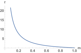
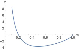
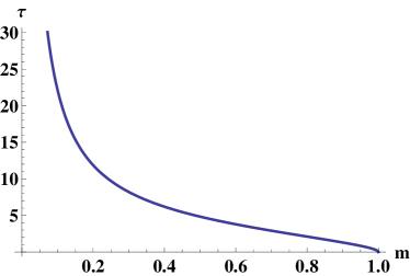
The behavior of $\tau$ is shown in figs 1a, 1b, corresponding to the cases $\lambda\geq 2$ and $0<\lambda<2$. In either case, as $m\to 0^{+}$, one has $\tau\approx\frac{2}{m}\to\infty$.

(a)	(b)

Figure 1: The relation between the width of the eigenvalue distribution and the coupling $\tau$ for given $\lambda$. In the interval $0<\lambda<2$, $\tau(m)$ has the form of figure (b). (a) $\lambda=4$. (b) $\lambda=1$.

Consider first $\lambda\geq 2$. Then $\tau$ is monotonic decreasing until $\tau=0$ at $m=1$. For any given $\lambda\geq 2$ and $\tau$, there is a unique $m$, hence a unique normalizable solution.

On the other hand, if $0<\lambda<2$, $\tau$ decreases up to a minimum value $\tau_{\rm min}<0$ and then increases monotonically until $\tau=0$ at $m=1$. In the region where $\tau>0$, there is a unique solution for $m$ for any given $0<\lambda<2$. On the other hand, in the region $\tau_{\rm min}<\tau<0$, there are two solutions for $m$ for a given $\tau$. However, the solution in the branch with higher $m$ is ruled out because $\rho$ becomes negative in two intervals $(\alpha_{1},\alpha_{0})$ and $(-\alpha_{0},-\alpha_{1})$ near the endpoint of the eigenvalue distribution.

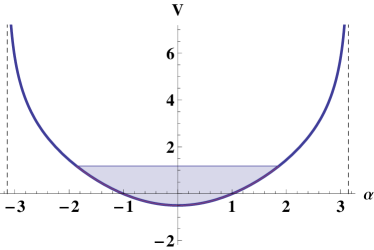
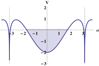
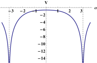
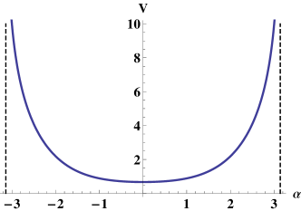
One surprising feature is that, when $\tau>0$, the gapped phase represented by the solution (40) exists all the way from $\lambda=0$ to $\lambda=\infty$. The reason can be understood from the potential, which goes to infinity as $\alpha=\pm\pi$ is approached (see fig. 3). This feature keeps the eigenvalues confined in a finite domain with $|\alpha_{0}|<\pi$ for all couplings $0<\lambda<\infty$ as long as $\tau>0$. As a result, the GWW phase transition disappears from the region $0<\lambda<\infty$ when a positive coupling $\tau$ is turned on. In other regions of the $(\lambda,\tau)$ parameter space there will be other phase transitions of different nature.

The transition to the region $\tau<0$ depends on the value of $\lambda$. For $0<\lambda<2$, one has $m<1$ so $\alpha_{0}<\pi$ (see fig. 1b); the solution (40) has no discontinuity in going from $\tau>0$ to $\tau<0$, i.e. from region I to region II of fig. 2. On the other hand, for $\lambda>2$, in the region $\tau\to 0^{+}$, one has $m\to 1^{-}$ and $\tau\approx\frac{\lambda-2}{\lambda}\,\sqrt{1-m}=\frac{\lambda-2}{\lambda}\,\cos\frac{\alpha_{0}}{2}$. The solution (40) becomes

$$\rho\to\frac{1}{2\pi}+\frac{1}{\pi\lambda}\,\cos\alpha\ ,\qquad\lambda>2,\ \tau\to 0^{+}\ .$$ (45)

Thus it matches continuously the ungapped solution (39) of the GWW model that exists on the half-line $\{\tau=0,\lambda>2\}$.

When $\tau$ is negative, the solution (40) exists in the shaded region II of fig. 2, $\tau_{\rm min}(\lambda)<\tau<0$ and $0<\lambda<2$, where $\tau_{\rm min}(\lambda)$ is the minimum of $\tau$ for a given $0<\lambda<2$ (fig. 1b). The curve separating regions II and III is $\tau_{\rm min}(\lambda)$ and it can be represented parametrically as follows

$$\tau=\frac{2(1-m)^{\frac{3}{2}}}{2-3m-2(1-m)^{\frac{3}{2}}}$$

(46)

$$\lambda=6m+4(1-m)^{\frac{3}{2}}-4\ ,\qquad 0<m<1\ .$$ (47)

On the critical curve, one has $m\to 1$ for $(\tau,2/\lambda)\to(0^{-},1)$. In the opposite limit, one has $m\to 0$ for $(\tau,2/\lambda)\to(\infty,\infty)$.

Because $m$ never reaches 1 for $\tau<0$ on the critical curve (i.e. $\alpha_{0}<\pi$), there cannot be a continuous transition to an ungapped phase across the critical line separating regions II and III. There is an ungapped phase in the GWW line at $\tau=0$ and $\lambda>2$, and also in region V. The solution is constructed below.

Figure 2: Partial representation of the phases of the theory in the region $\lambda>0$. The one-cut solution (40) exists in the shaded regions I and II. In region IV the minimum of the potential at $\alpha=0$ has disappeared. The ungapped solution (48) exists in region V. It matches continuously on the red dashed vertical line with the solution at $\tau\geq 0$.

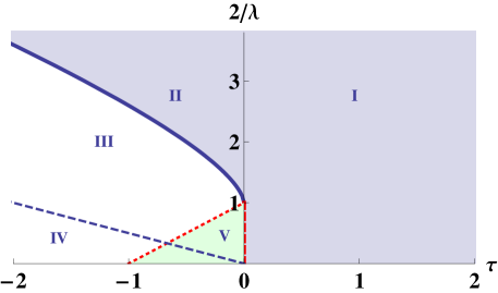
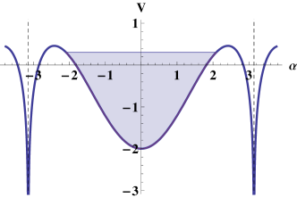
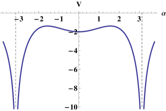
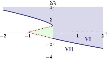
The phase diagram of fig. 2 summarizes the different regimes of the theory with $\lambda>0$. An interesting question is what is the solution in regions III and IV. The new solution must match continuously the solution (40) on the critical line separating regions II and III. A hint on the nature of the new phases is provided by the form of the potential in the different regions:

• In region I, the potential is shown in fig. 3. It goes to infinity as $\alpha=\pm\pi$ is approached, which explains why for $\tau>0$ there is never a transition to an ungapped solution.

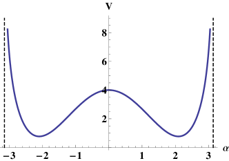
• In region II, the potential has the form of fig. 4a. As the critical line is approached, eigenvalues almost fill the well, indicating a possible transition to a solution where part of the eigenvalues sit on the wells at $\pm\pi$.

• Finally, figs. 5a, b represent the potential in regions III and IV. They suggest the existence of a critical line near the dashed line in fig. 2 where there is a transition to a solution where all eigenvalues sit on the wells at $\pm\pi$.

Let us now describe the ungapped solution where eigenvalues are spread over the whole circle, $\alpha_{0}=\pi$. The normalized solution is given by

$$\rho(\alpha)=\frac{(1+\tau)}{2\pi}+\frac{1}{\pi\lambda}\cos\alpha-\frac{1}{2}\tau\left(\delta(\alpha-\pi)+\delta(\alpha+\pi)\right)\ .$$ (48)

The solution continuously matches the GWW solution (39) on the half-line $\tau=0$, $\lambda>2$, which also matches the solution (40) in region I at $\tau\to 0^{+}$, $\lambda>2$. The critical line separating the region where this solution exists can be found from the requirement that $\rho$ is non-negative in the whole interval $[-\pi,\pi)$. This gives the condition

$$\tau+1>\frac{2}{\lambda}>-\tau-1\ .$$ (49)

The complete relevant region for this phase is shown in fig. 9.

Figure 3: Potential in region I (here $\lambda=4$, $\tau=1$).

(a)	(b)

Figure 4: Potential. (a) $\tau=-0.3,\lambda=1$, corresponding to region II. (b) $\tau=-0.5,\lambda=1$, $\alpha_{0}=2\pi/3$, corresponding to the critical line separating region II and region III.

(a)	(b)

Figure 5: Potential. (a) $\tau=-2$, $\lambda=1$ corresponding to region III. (b) $\tau=-2$, $\lambda=3$, corresponding to region IV.

3.2 Case $\lambda<0$

The solution (40) still holds in part of the region $\lambda<0$, $\tau>0$. For all $\lambda<0$, provided $\tau>0$, there is a unique solution $m(\lambda,\tau)$ to the normalization condition for each pair $(\lambda,\tau)$. This is shown in fig. 6. On the other hand, there is no solution for $\tau<0$, so the phase described by the solution (40) does not exist in the quadrant $(\lambda<0,\tau<0)$. In this quadrant eigenvalues should condense on a cut near the wells at $\pm\pi$. We expect a smooth transition from region IV of fig. 2, since the potential is qualitatively the same.

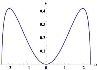
Thus, let us consider the quadrant $(\lambda<0,\tau>0)$. Starting with large $|\lambda|$, the potential has an absolute minimum at $\alpha=0$ and it develops a double well for a coupling $\lambda>\lambda_{1}$, $\lambda_{1}=-4/\tau$ (see fig. 7). Therefore one expects a phase transition where the eigenvalue distribution splits in two cuts, at some critical coupling $\lambda_{\rm cr}>\lambda_{1}$ (i.e. $|\lambda_{\rm cr}|<|\lambda_{1}|$). This phase transition is nothing but the unitary model version of the phase transition described in Russo:2020pnv for the corresponding Hermitian matrix model (8). The eigenvalue density may be found from the two-cut solution in Russo:2020pnv by using the duality map between Hermitian and unitary models Mizoguchi:2004ne (see also Okuyama:2017pil ). However, in this paper we will not explore this region.

Figure 6: $\tau$ in terms of $m$ given by (44) (here $\lambda=-1$). For any given $\tau>0$ and $\lambda<0$ there is a unique solution $m$ to the normalization condition.

(a)	(b)

Figure 7: Potential. (a) $\tau=2,\lambda=-3$, corresponding to region VI with $\lambda<\lambda_{\rm cr}$. (b) $\tau=2,\lambda=-0.5$, corresponding to region VII with $\lambda>\lambda_{\rm cr}$.

(a)	(b)

Figure 8: Eigenvalue density. (a) $\tau=2,\lambda=-1$, corresponding to region VI. (b) $\tau=2,\lambda=\lambda_{\rm cr}(\tau=2)$, corresponding to the critical line. For higher $\lambda$, the eigenvalues split in a two-cut distribution.

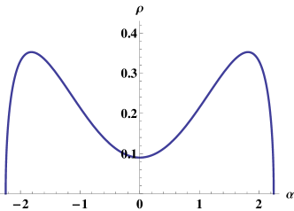
Like in Russo:2020pnv , the critical line occurs when the eigenvalue density vanishes at $\alpha=0$ (see fig. 8b). This gives the equation

$$\lambda\tau=-4\sqrt{1-m}\ .$$

Hence $|\lambda_{\rm cr}/\lambda_{1}|<1$, which means that the phase transition does not occur immediately when the double well forms, but for a greater $\lambda$. When $\lambda$ overcomes $\lambda_{1}=-4/\tau$, there is still a one-cut solution due to overfilling of eigenvalues fully covering the two wells. At $\lambda>\lambda_{\rm cr}$, the eigenvalues get separated in two sets filling part of each well. Combining with (44) – which implicitly determines $m$ in terms of $\lambda,\ \tau$, we find the critical line

$$\lambda_{\rm cr}=-\frac{4}{\tau^{2}}\left(\tau-\sqrt{2\tau+1}+1\right)\ .$$ (50)

For $\tau\to\infty$, one has $m\to 0$ and $\lambda\approx-4/\tau$. In the opposite limit, for $\tau\to 0^{+}$, one has $m\approx 1$ and $\lambda_{\rm cr}\to-2$. This is expected, since, as explained above, when $\tau=0$ the theory with $\lambda<0$ is equivalent to the theory in the interval $\lambda>0$ and thus it has a GWW phase transition at $\lambda=-2$.

Viewing the $\lambda<0$ model as the standard GWW model with $\lambda>0$ deformed by $2\tau\ln|\sin\frac{\alpha}{2}|$, one can get another insight on the origin of the two-cut solution. This deformation makes the potential to go to $+\infty$ as $\alpha\to 0$; as a result, the eigenvalue distribution – that for $\tau=0$ and small $\lambda$ would have support in a cut near $\alpha=0$ – now necessarily splits into two cuts. On the other hand, for strong $\lambda$, the eigenvalue distribution, that in the $\tau=0$ theory would cover the whole circle, now must have a gap near $\alpha=0$ due to the infinite wall. Therefore, in the GWW model with $\lambda>0$ deformed by $2\tau\ln|\sin\frac{\alpha}{2}|$ the GWW phase transition extends to the full critical line $|\lambda_{\rm cr}(\tau)|$. For any $\tau>0$, the phase transition now involves a transition between a solution with two gaps and a solution with one gap.

The resulting phase diagram is shown in fig. 9.

Figure 9: Phase diagram. The gapped phase described by solution (40) exists in the grey shaded region. The green shaded area describes the region V where the ungapped phase solution (48) exists. Below the critical line $\lambda_{\rm cr}$ in region VII there is a two-cut phase where eigenvalues accumulate at the two minima of the potential (c.f. fig. 7b).

3.3 Free energy and Wilson loops

Here we use the eigenvalue densities (40) and (48) to compute the free energy in regions I, II, V and VI. By differentiating with respect to $\lambda$, one obtains a formula for the VEV of the Wilson loop:

$$\langle W\rangle=\frac{\lambda^{2}}{2N^{2}}\frac{\partial F}{\partial\lambda}=\langle\cos\alpha\rangle\ .$$ (51)

Let us first consider the eigenvalue density (40). Computing the integrals we find

$$\langle W\rangle=\int_{-\alpha_{0}}^{\alpha_{0}}d\alpha\ \rho(\alpha)\ \cos\alpha\ =\frac{1}{\lambda}m(2-m)+\tau\left(1-\sqrt{1-m}\right)\ .$$ (52)

The dependence of the Wilson loop as a function of the couplings $\lambda$ and $\tau$ is complicated, because $m(\lambda,\tau)$ is a solution of a cubic equation. However, we can expand $\langle W\rangle$ in series to exhibit the small $\lambda$ and the small $\tau$ behavior. At small $\lambda>0$, one has the expansion

$$\langle W\rangle=1-\frac{\lambda}{4}+\frac{\lambda^{2}\tau}{16}+\frac{1}{64}\lambda^{3}\left(\tau-\tau^{2}\right)+\frac{\lambda^{4}\left(4\tau^{3}-12\tau^{2}+5\tau\right)}{1024}+O\left(\lambda^{5}\right)\ .$$ (53)

At small $\tau$ and in the region $0<\lambda<2$, one has the expansion

$$m=\frac{\lambda}{2}+\frac{\lambda\left(2-\lambda-\sqrt{4-2\lambda}\right)\tau}{2(2-\lambda)}+\frac{\left(2-\sqrt{4-2\lambda}\right)\lambda^{2}\tau^{2}}{4(2-\lambda)^{2}}+O\left(\tau^{3}\right)\ ,$$ (54)

and

$$\langle W\rangle=1-\frac{\lambda}{4}+\left(2-\frac{\lambda}{2}-\sqrt{4-2\lambda}\right)\tau+\frac{\lambda\left(\lambda+2\sqrt{4-2\lambda}-4\right)\tau^{2}}{4(2-\lambda)}+O\left(\tau^{3}\right)\ .$$ (55)

The first term in (55) is of course the VEV of the Wilson loop in the GWW model in the weak coupling phase. The second term displays the non-analytic behavior at the GWW critical point $\lambda=2$.

Let us now consider the regions where $\lambda>2$. In this region the parameter $m$ solving the normalization condition (42) has the small $\tau$ expansion

$$m=1-\frac{\lambda^{2}\tau^{2}}{(\lambda-2)^{2}}+O\left(\tau^{3}\right)\ .$$ (56)

This gives

$$\langle W\rangle=\frac{1}{\lambda}+\tau-\frac{\lambda}{\lambda-2}\,\tau^{2}+O\left(\tau^{3}\right)\ .$$ (57)

For $\tau\to 0$, this agrees with the VEV of the Wilson loop of GWW theory in the strong coupling phase.

Another useful observable is

$$-\frac{1}{N^{2}}\frac{\partial F}{\partial\tau}=\langle\ln\cos^{2}\frac{\alpha}{2}\rangle=\int_{-\alpha_{0}}^{\alpha_{0}}d\alpha\ \rho(\alpha)\ \ln\cos^{2}\frac{\alpha}{2}\,.$$ (58)

The order of a phase transition is determined by the continuity properties of the derivatives of the free energy in crossing a critical line in $(\lambda,\tau)$ space. In particular, for a third-order phase transition, the second derivatives $\partial^{2}_{\tau}F$, $\partial^{2}_{\lambda}F$ and $\partial_{\lambda}\partial_{\tau}F$ must be continuous. Hence this observable and $\langle W\rangle$ are instrumental in order to classify the different types of transitions occurring in $(\lambda,\tau)$ space. Computing the integral, we obtain

$$-\frac{1}{N^{2}}\frac{\partial F}{\partial\tau}=\frac{1}{\lambda}J_{1}+\tau J_{2}\ ,$$ (59)

with

$$J_{1}=4-4\sqrt{1-m}-2m\left(1-2\log\frac{1}{2}\left(1+\sqrt{1-m}\right)\right)\ ,$$

(60)

$$J_{2}=-\left(\frac{1}{\sqrt{1-m}}+1\right)\log\left(\frac{4\left(2-m-2\sqrt{1-m}\right)}{m^{2}}\right)-\log(1-m)\ .$$ (61)

In the region $\lambda>2$, one finds the small $\tau$ expansion,

$$-\frac{1}{N^{2}}\frac{\partial F}{\partial\tau} = \frac{2}{\lambda}-\log 4+\tau\left(\log\frac{(\lambda-2)^{2}}{16\tau^{2}\lambda^{2}}+2\right)$$ (62)

$$+ \frac{\lambda\tau^{2}(3\lambda(1-\log 2)-6+10\log 2)}{(\lambda-2)^{2}}+O\left(\tau^{3}\right)$$

We can check that (57) and (62) satisfy the integrability condition $\partial_{\lambda}\partial_{\tau}F=\partial_{\tau}\partial_{\lambda}F$.

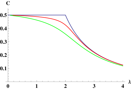
The critical behavior of the free energy can be studied by expanding these expressions near critical lines. As a first example, we consider the GWW phase transition. We have seen that there is no critical line when $\tau>0$ and that the phase transition becomes a cross-over. Figure 10 illustrates how the phase transition is smoothed out, by means of a plot of the “specific heat” $C=dE/d\lambda$, $E=\lambda^{2}\partial F/\partial\lambda=2N^{2}\langle W\rangle$ in terms of the “temperature” $\lambda$. This shows that $\partial_{\lambda}^{2}F$ is smooth for $\tau>0$. A similar behavior is observed for $\partial_{\tau}\partial_{\lambda}F$ and $\partial_{\tau}^{2}F$.

Figure 10: Specific heat $C/N^{2}=-2\partial_{\lambda}W$ as a function of $\lambda$. From top to bottom, $\tau=0$, $\tau=0.03$ and $\tau=0.1$.

As a second example, let us discuss the phase transition across the critical line defined by $\{\tau=0,\ \lambda>2\}$ in going from positive $\tau$ to negative $\tau$. This is a rather drastic transition, since the potential has infinite wells on the other side, in region V. Nevertheless, from a mathematical viewpoint, it is interesting to examine analytic properties in going across this line. We need the first derivatives of the free energy with respect to the couplings $\lambda$ and $\tau$ in region V, where the eigenvalue density is given by (48). In this phase the integrals are very simple and we obtain

$$\langle W\rangle=\frac{1}{\lambda}+\tau\ ,$$ (63)

$$-\frac{1}{N^{2}}\frac{\partial F}{\partial\tau}=\langle\ln\cos\frac{\alpha}{2}\rangle=\frac{2}{\lambda}-\log 4-\tau\log 4-\tau\ln\cos\frac{\pi-\epsilon}{2}\ .$$ (64)

We see that, in phase V, the VEV of $\ln\cos\frac{\alpha}{2}$ has a logarithmic singularity, which here has been regularized with a cutoff $\epsilon>0$. Note also the crucial role of the $\delta$ function term in the density (48) to produce the $\tau$ term in $\langle W\rangle$, which is required by the integrability condition $\partial_{\lambda}\partial_{\tau}F=\partial_{\tau}\partial_{\lambda}F$. From the small $\tau$ expansions, we see that $\partial_{\lambda}F$ and $\partial_{\tau}F$ are continuous across the $\tau=0$ line. Likewise, $\partial^{2}_{\lambda}F$ and $\partial_{\lambda}\partial_{\tau}F$ are also continuous. However, $\partial^{2}_{\tau}F$ is discontinuous. This indicates that the phase transition across the $\tau=0$ line in going from phase V to phase I (or to phase VI) is second order.

One can similarly compute the VEV of winding Wilson loops $W_{k}=\cos k\alpha$. In particular, in the gapped phase described by (40), we find

$$\langle\cos 2\alpha\rangle=\frac{2m(1-m)^{2}}{\lambda}+\left((1+m)\sqrt{1-m}-1\right)\tau\ ,$$

$$\langle\cos 3\alpha\rangle=\frac{m(2-5m)(1-m)^{2}}{\lambda}-\left((2m^{2}+1)\sqrt{1-m}-1\right)\tau\ ,$$ (65)

etc. Near the critical line $\{\tau=0,\ \lambda>2\}$, one can use the expansion (56) to find a general formula for the near critical behavior:

$$\langle\cos k\alpha\rangle=(-1)^{k+1}\ \tau\left(1-\frac{k\lambda}{(\lambda-2)}\tau+O\left(\tau^{2}\right)\right)\ ,\qquad k=1,2,\cdots$$ (66)

This can be compared with the result in the ungapped phase, i.e. on the other side of the transition. Using (48), we find

$$\langle W_{k}\rangle=(-1)^{k+1}\ \tau\ .$$ (67)

Comparing with (66), we see that all $W_{k}$ and $\partial_{\tau}W_{k}$ are continuous as functions of $\tau$ at $\tau=0$, but the second derivatives $\partial^{2}_{\tau}W_{k}$ are discontinuous. Once again, note the crucial role of the delta function terms in (48), this time to ensure continuity of $\partial_{\tau}W_{k}$.

In conclusion, we have seen that the theory has a complicated phase structure. It is clear that much deeper analysis is required to establish the dominant phases in each region and, in particular, to determine the order of phase transitions that occur when crossing the different critical lines. If we restrict ourselves to the “physical” $\tau>0$ region, the phase structure seems to be simpler, with a single phase transition from region VI to region VII, which can be thought of as the extension of the GWW phase transition in the presence of the $\tau$ coupling (analogous to the liquid-vapor phase transition, in a phase diagram that includes temperature and pressure). The transition should be of the third order, being the counterpart of the third-order phase transition found in Russo:2020pnv in the dual Hermitian model. We leave these problems for future work.

4 Discussion

The generalized GWW matrix theory studied in this work may be viewed as two-dimensional lattice gauge theory with an insertion

$$\hat{O}^{\nu}\ ,\qquad\hat{O}\equiv\frac{1}{4}\det(1+U)\det(1+U^{\dagger})\ ,$$ (68)

in the plaquette partition function, arising after the axial gauge choice. A relevant open problem is to see if this deformation of the GWW model can arise in a natural way in the context of the original 2d lattice gauge theory (for example, by starting with a Hamiltonian of the Kogut-Susskind type). Clearly, a deeper understanding of a possible lattice gauge theory origin of the model is desirable. This seems relevant considering also that low dimensional lattice gauge theories are being understood nowadays with modern tools from quantum information theory (such as matrix product states or tensor networks) and from the point of view of quantum simulation Banuls:2019bmf .

Alternatively, one could view the $\tau$ deformed matrix model as a phenomenological model which may incorporate some interesting physical features of gauge theory. The most dramatic effect of the deformation is to smooth out the GWW phase transition. For any small positive $\tau$, the transition becomes a cross-over. As a result, there is no ungapped phase where eigenvalues get distributed over the whole circle in the “physical” region $\tau>0$. In addition, there are many new features in other regions of parameter space, including various phase transitions, which, perhaps, could eventually find some interesting physical interpretation in the context of gauge theory.

In particular, in the $\lambda<0$ region the deformation has a different effect. We recall that one can switch the sign of $\lambda$ by a formal shift in the angular variables and view the model as the usual GWW model with $\lambda>0$ deformed by a $2\tau\ln|\sin\frac{\varphi}{2}|$ term in the potential. This corresponds to the insertion of an operator

$$\tilde{O}^{\nu}\ ,\qquad\tilde{O}\equiv\frac{1}{4}\det(1-U)\det(1-U^{\dagger})\ .$$ (69)

With this deformation, the GWW transition extends to a critical line $|\lambda_{\rm cr}(\tau)|$, given in (50), and in the new phase eigenvalues get distributed into two separated, symmetric cuts. This is the counterpart of the third order phase transition found in the dual Hermitian model Russo:2020pnv .

An interesting question is if all phases appearing in the whole $(\lambda,\tau)$ parameter space have a counterpart in the Hermitian model of Russo:2020pnv . The correspondence in the phase structure of unitary and Hermitian matrix models in the large $N$ limit involves subtle issues that have been recently discussed in Santilli:2020ueh . In the present model, the main difference will occur in the $\tau<0$ region. In the unitary model there are normalizable solutions with eigenvalues sitting at the wells $\pm\pi$; in the Hermitian model eigenvalues will be spread to infinity and the corresponding solution would not be normalizable. In some unitary models the underlying mechanism triggering some phase transitions may be different. See for example a discussion in Appendix (B.1) in Santilli:2018byi .

It would also be very interesting to understand the contribution of large $N$ instantons by computing complex saddle-points. This analysis was carried out only recently for the GWW model Buividovich:2015oju ; Alvarez:2016rmo (see also Okuyama:2017pil ). The GWW model describes certain quantum amplitudes of the XX spin chain model Perez-Garcia:2013lba . If $B=\mathrm{i}t$ with $t$ real, the amplitude is related to real-time dynamics of the spin chain model, but then there is no phase transition spinchain . In general, it is relevant, in that context, to study the case of a GWW model with a complex parameter spinchain ; Santilli:2018byi . It would then be interesting to study the eventual phase structure for imaginary or even complex values of at least one of the parameters of the model.

In addition to lattice gauge theory and spin chain models, there are a number of extremely insightful applications of the GWW model in low-energy QCD Leutwyler:1992yt ; Verbaarschot:2005rj . In that context, insertions of the characteristic polynomial type, such as (68), appear often. In the specific case of the GWW model, a simpler insertion of the form $\det(U)^{\nu}$ (which has an interpretation as a topological term) has been considered in Rossi:1996hs ; Leutwyler:1992yt ; Verbaarschot:2005rj ,

Acknowledgements

J.G.R. acknowledges financial support from projects 2017-SGR-929, MINECO grant FPA2016-76005-C. The work of MT was partially supported by the Fundação para a Ciência e a Tecnologia (FCT) through FCT Project PTDC/MAT-PUR/30234/2017.

References

- (1) M. L. Mehta, Random Matrices, Pure and Applied Mathematics. Elsevier Science, 2004.
- (2) P. J. Forrester, “Log-gases and random matrices”, London Mathematical Society Monographs Series, vol. 34 (Princeton University Press. Princeton, NJ, 2010).
- (3) J. Baik, P. Deift and T. Suidan, Combinatorics and random matrix theory, vol. 172 of Graduate Studies in Mathematics. American Mathematical Society, Providence, RI, (2016).
- (4) D. Gross and E. Witten, “Possible Third Order Phase Transition in the Large N Lattice Gauge Theory,” Phys. Rev. D 21, 446-453 (1980)
- (5) S. R. Wadia, “A Study of U(N) Lattice Gauge Theory in 2-dimensions,”, [arXiv:1212.2906 [hep-th]].
- (6) S. R. Wadia, “ = Infinity Phase Transition in a Class of Exactly Soluble Model Lattice Gauge Theories,” Phys. Lett. B 93, 403-410 (1980)
- (7) J. Baik, P. Deift, K. Johansson, “On the distribution of the length of the longest increasing subsequence of random permutations,” Journal of the American Mathematical Society, 12(4), 1119-1178, (1999), [arXiv:math/9810105 [math.CO]]
- (8) D. Romik, “The surprising mathematics of longest increasing subsequences,” Vol. 4. Cambridge University Press, (2015).
- (9) A. Böttcher, S. M. Grudsky, “Spectral properties of banded Toeplitz matrices.” Society for Industrial and Applied Mathematics (2005).
- (10) C. A. Tracy and H. Widom, “On the distributions of the lengths of the longest monotone subsequences in random words,” Probab. Theory Related Fields, 119 (3), 350-380 (2001), [arXiv:math/9904042]
- (11) J. G. Russo, “Deformed Cauchy random matrix ensembles and large phase transitions,” [arXiv:2006.00672 [hep-th]].
- (12) N. S. Witte and P. J. Forrester, “Gap probabilities in the finite and scaled Cauchy random matrix ensembles,” Nonlinearity 13 (2000) 1965-1986, [arXiv:math-ph/0009022].
- (13) A. Böttcher, B. Silbermann, “Toeplitz matrices and determinants with Fisher-Hartwig symbols,” Journal of functional analysis, 63(2), 178-214 (1985).
- (14) A. Ahmed and G. V. Dunne, “Non-perturbative large trans-series for the Gross–Witten–Wadia beta function,” Phys. Lett. B 785, 342-346 (2018) [arXiv:1808.05236 [hep-th]].
- (15) A. Ahmed and G. V. Dunne, “Transmutation of a Trans-series: The Gross-Witten-Wadia Phase Transition,” JHEP 11, 054 (2017) [arXiv:1710.01812 [hep-th]].
- (16) D. García-García and M. Tierz. “Toeplitz minors and specializations of skew Schur polynomials,” Journal of Combinatorial Theory, Series A 172 (2020): 105201, [arXiv:1706.02574 [math.CO]].
- (17) P. Deift, A. Its, and I. Krasovsky, “Toeplitz Matrices and Toeplitz Determinants under the Impetus of the Ising Model: Some History and Some Recent Results,” Communications on Pure and Applied Mathematics 66, no. 9 (2013): 1360-1438, [arXiv:1207.4990 [math.FA]].
- (18) P. Rossi, M. Campostrini and E. Vicari, “The Large N expansion of unitary matrix models,” Phys. Rept. 302, 143-209 (1998) [arXiv:hep-lat/9609003 [hep-lat]].
- (19) K. Okuyama, “Wilson loops in unitary matrix models at finite ,” JHEP 07, 030 (2017) [arXiv:1705.06542 [hep-th]].
- (20) E. Alfinito and M. Beccaria, “Large expansion of Wilson loops in the Gross-Witten-Wadia matrix model,” J. Phys. A 51, no.5, 055401 (2018) [arXiv:1707.09625 [hep-th]].
- (21) S. Mizoguchi, “On unitary / hermitian duality in matrix models,” Nucl. Phys. B 716 (2005), 462-486 [arXiv:hep-th/0411049 [hep-th]].
- (22) M. C. Bañuls et al., “Simulating Lattice Gauge Theories within Quantum Technologies,” [arXiv:1911.00003 [quant-ph]].
- (23) L. Santilli and M. Tierz, “Exact equivalences and phase discrepancies between random matrix ensembles,” [arXiv:2003.10475 [math-ph]], J. Stat. Mech. (JSTAT) in press.
- (24) L. Santilli and M. Tierz, “Phase transitions and Wilson loops in antisymmetric representations in Chern–Simons-matter theory,” J. Phys. A 52, no.38, 385401 (2019) [arXiv:1808.02855 [hep-th]].
- (25) P. V. Buividovich, G. V. Dunne and S. N. Valgushev, “Complex Path Integrals and Saddles in Two-Dimensional Gauge Theory,” Phys. Rev. Lett. 116, no.13, 132001 (2016) [arXiv:1512.09021 [hep-th]].
- (26) G. Álvarez, L. Martínez Alonso and E. Medina, “Complex saddles in the Gross-Witten-Wadia matrix model,” Phys. Rev. D 94 (2016) no.10, 105010 [arXiv:1610.09948 [hep-th]].
- (27) D. Pérez-García and M. Tierz, “Mapping between the Heisenberg XX Spin Chain and Low-Energy QCD,” Phys. Rev. X 4, no.2, 021050 (2014) [arXiv:1305.3877 [cond-mat.str-el]].
- (28) L. Santilli and M. Tierz, “Phase transition in complex-time Loschmidt echo of short and long range spin chain,” Journal of Statistical Mechanics: Theory and Experiment 2020, no. 6 (2020) 063102, [arXiv:1902.06649 [cond-mat.stat-mech]].
- (29) H. Leutwyler and A. V. Smilga, “Spectrum of Dirac operator and role of winding number in QCD,” Phys. Rev. D 46, 5607-5632 (1992)
- (30) J. J. M. Verbaarschot, “QCD, chiral random matrix theory and integrability,” [arXiv:hep-th/0502029 [hep-th]].