The miniJPAS survey: star-galaxy classification using machine learning

Abstract

Context. Future astrophysical surveys such as J-PAS will produce very large datasets, the so-called “big data”, which will require the deployment of accurate and efficient Machine Learning (ML) methods. In this work, we analyze the miniJPAS survey, which observed about $\sim$$1\text{deg}^{2}$ of the AEGIS field with 56 narrow-band filters and 4 $ugri$ broad-band filters. The miniJPAS primary catalogue contains approximately 64000 objects in the $r$ detection band (mag${}_{AB}\lesssim 24$), with forced-photometry in all other filters.

Aims. We discuss the classification of miniJPAS sources into extended (galaxies) and point-like (e.g. stars) objects, a necessary step for the subsequent scientific analyses. We aim at developing an ML classifier that is complementary to traditional tools based on explicit modeling. In particular, our goal is to release a value added catalog with our best classification.

Methods. In order to train and test our classifiers, we crossmatched the miniJPAS dataset with SDSS and HSC-SSP data, whose classification is trustworthy within the intervals $15\leq r\leq 20$ and $18.5\leq r\leq 23.5$, respectively. We trained and tested 6 different ML algorithms on the two crossmatched catalogs: K-Nearest Neighbors (KNN), Decision Trees (DT), Random Forest (RF), Artificial Neural Networks (ANN), Extremely Randomized Trees (ERT) and Ensemble Classifier (EC). EC is a hybrid algorithm that combines ANN and RF with J-PAS’s stellar/galaxy loci classifier (SGLC). As input for the ML algorithms we use the magnitudes from the 60 filters together with their errors, with and without the morphological parameters. We also use the mean PSF in the $r$ detection band for each pointing.

Results. We find that the RF and ERT algorithms perform best in all scenarios. When analyzing the full magnitude range of $15\leq r\leq 23.5$ we find $AUC=0.957$ (area under the curve) with RF when using only photometric information, and $AUC=0.986$ with ERT when using photometric and morphological information. Regarding feature importance, when using morphological parameters, FWHM is the most important feature. When using photometric information only, we observe that broad bands are not necessarily more important than narrow bands, and errors (the width of the distribution) are as important as the measurements (central value of the distribution). In other words, the full characterization of the measurement seems to be important.

Conclusions. ML algorithms can compete with traditional star/galaxy classifiers, outperforming the latter at fainter magnitudes ($r\gtrsim 21$). We use our best classifiers, with and without morphology, in order to produce a value added catalog available at j-pas.org/datareleases via the ADQL table minijpas.StarGalClass. The ML models are available at github.com/J-PAS-collaboration/StarGalClass-MachineLearning.

1 Introduction

An important step in the analysis of data from wide-field surveys is the classification of sources into stars and galaxies. Although challenging, this separation is crucial for many areas of cosmology and astrophysics. Different classification methods have been proposed in the literature, each having their respective advantages and disadvantages. One of the most used methods is based on morphological separation, where parameters related to the object structure and photometry are used (Bertin & Arnouts, 1996; Henrion et al., 2011; Molino et al., 2014; Díaz-García et al., 2019; López-Sanjuan et al., 2019). In these methods one assumes that stars appear as point sources while galaxies as extended sources. This has been shown to be consistent with previous spectroscopic observations (Le Fevre et al., 1995; Dawson et al., 2013; Newman et al., 2013). However, at fainter magnitudes, the differences between these point-like and extended structures decrease and this method becomes unreliable. In what follows, by “stars” we mean point-like objects that are not galaxies, that is, both stars and quasars.

Future photometric surveys such as the Javalambre-Physics of the Accelerating Universe Astrophysical Survey (J-PAS, Benitez et al., 2014) and the Vera Rubin Observatory Legacy Survey of Space and Time (LSST, Marshall et al., 2017) will detect a large number of objects and are facing the management of data produced at an unprecedented rate. The LSST, in particular, will reach a rate of petabytes of data per year (Garofalo et al., 2016). This wealth of data demands very efficient numerical methods but also gives us the opportunity to deploy Machine Learning (ML) algorithms, which, trained on big astronomical data, have the potential to outperform traditional methods based on explicit programming, if biases due to potentially unrepresentative training sets are kept under control.

ML has been widely applied in the context of cosmology and astrophysics, see Ishak (2017). A non-exhaustive list of applications is photometric classification of supernovae (Lochner et al., 2016; Charnock & Moss, 2017; Vargas dos Santos et al., 2020), gravitational wave analysis (Biswas et al., 2013; Carrillo et al., 2015), photometric redshift (Bilicki et al., 2018; Cavuoti et al., 2015), morphology of galaxies (Gauci et al., 2010; Banerji et al., 2010), and determination of atmospheric parameters for stellar sources (Whitten et al., 2019).

ML applications to star-galaxy separation have been successfully performed on many surveys. Vasconcellos et al. (2011), for example, used various tree methods to classify SDSS sources. Kim et al. (2015) used classifiers that mix supervised and unsupervised ML methods with CFHTLenS data. Recently, Convolutional Neural Networks (CNN) have been adopted: using images as input, they achieve an Area Under the Curve (AUC) ¿ 0.99 for CFHTLenS and SDSS data (Kim & Brunner, 2017). For more ML applications in the context of star/galaxy classification see Costa-Duarte et al. (2019); Sevilla-Noarbe et al. (2018); Cabayol et al. (2019); Fadely et al. (2012); Odewahn et al. (2004).

Our goal here is to classify the objects detected by Pathfinder miniJPAS (Bonoli et al., 2020), which observed $\sim$$1\text{deg}^{2}$ of the AEGIS field with the 56 narrow-band J-PAS filters and the 4 $ugri$ broad-band filters, for a total of approximately 64000 objects (mag${}_{AB}\lesssim 24$). The ML algorithms that we consider in this work are supervised and, for the learning process, need an external trustworthy classification. We adopt Sloan Digital Sky Survey (SDSS, Alam et al., 2015) and Hyper Suprime-Cam Subaru Strategic Program (HSC-SSP, Aihara et al., 2019) data. We compare different ML models to each other and to the two classifiers adopted by the JPAS survey: the CLASS_STAR provided by SExtractor (Bertin & Arnouts, 1996) and the stellar/galaxy loci classifier (SGLC) introduced in López-Sanjuan et al. (2019).

This paper is organized as follows. In Section 2, we briefly describe J-PAS and miniJPAS and we review the classifiers adopted in miniJPAS. In Section 3 we present the ML algorithms used in this work, and in Section 4 we define the metrics that we use to assess the performance of the classifiers. Our results are presented in Sections 5 and 5.3, and our conclusions in Section 6.

2 J-PAS and miniJPAS

J-PAS is a ground-based imaging survey that will observe 8500 deg² of the sky via the technique of quasi-spectroscopy: by observing with 56 narrow-band filters and 4 $ugr(i)$ broad-band filters it will produce a pseudo-spectrum ($R\sim 50$) for every pixel (for the filters’ specifications see Bonoli et al., 2020). It features a dedicated 2.5m telescope with an excellent étendue, equipped with a 1.2 Gigapixel camera with a very large field of view of $4.2\deg^{2}$. The observatory is on the mountain range “Sierra de Javalambre” (Spain), at an altitude of approximately 2000 meters, an especially dark region with the very good median seeing of $0.7^{\prime\prime}$ (Cenarro et al., 2010). Therefore, J-PAS sits between photometric and spectroscopic surveys, fruitfully combining the advantages of the former (speed and low cost) with the ones of the latter (spectra). In particular, thanks to its excellent photo-$z$ performance, it will be possible to accurately study the large scale structure of the universe using the galaxy and quasar catalogs produced by J-PAS (Bonoli et al., 2020).

Between May and September 2018, the 2.5m J-PAS telescope with its filter set was equipped with the Pathfinder camera, used to test the telescope performance and execute the first scientific operations. The camera features a 9k $\times$ 9k CCD, with a 0.3 deg² field-of-view and 0.225 arcsec pixel size. This led to the miniJPAS survey which covered a total of $\sim 1\text{deg}^{2}$ of the AEGIS field, reaching the target depth planned for J-PAS (mag_AB, 5$\sigma$ in a 3” aperture, between 21.5 and 22.5 for the narrow-band filters and up to 24 for the broad-band filters). miniJPAS consists of the 4 fields/pointings AEGIS1-4, each of approximately 0.25 deg² field-of-view. The miniJPAS primary catalogue contains 64293 objects in the $r$ detection band, with forced-photometry in all other filters. See Bonoli et al. (2020) for the presentation paper. The miniJPAS Public Data Release was presented to the public in December 2019.

2.1 Crossmatched catalogs

Figure 1: Histograms of the $r$-band magnitudes of the sources of the miniJPAS catalog crossmatched with the SDSS (top) and HSC-SSP (bottom) catalogs. Classification by SDSS and HSC-SSP, respectively. Galaxies are shown in red, stars in semi-transparent blue.

Figure 2: Histograms of the photometric redshifts of the galaxies of the miniJPAS catalog crossmatched with the SDSS (semi-transparent purple) and HSC-SSP (green) catalogs.

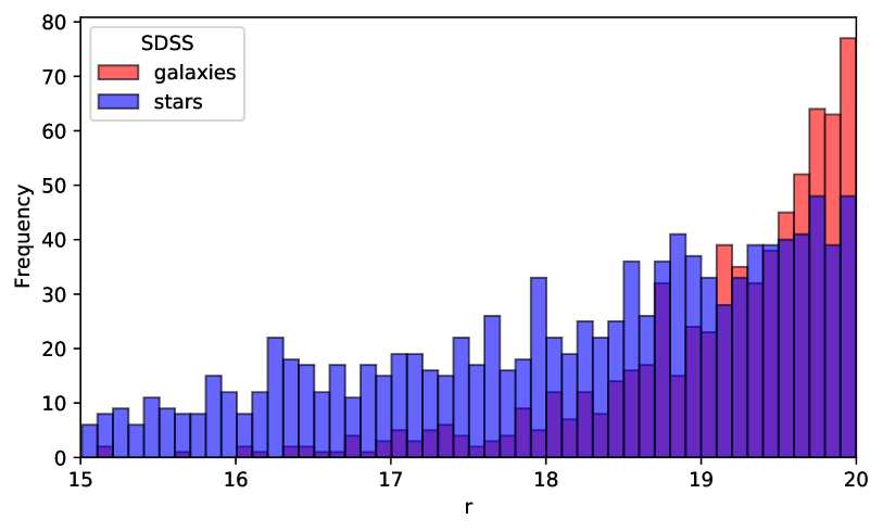
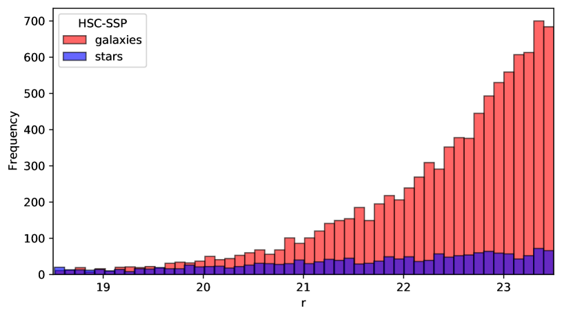
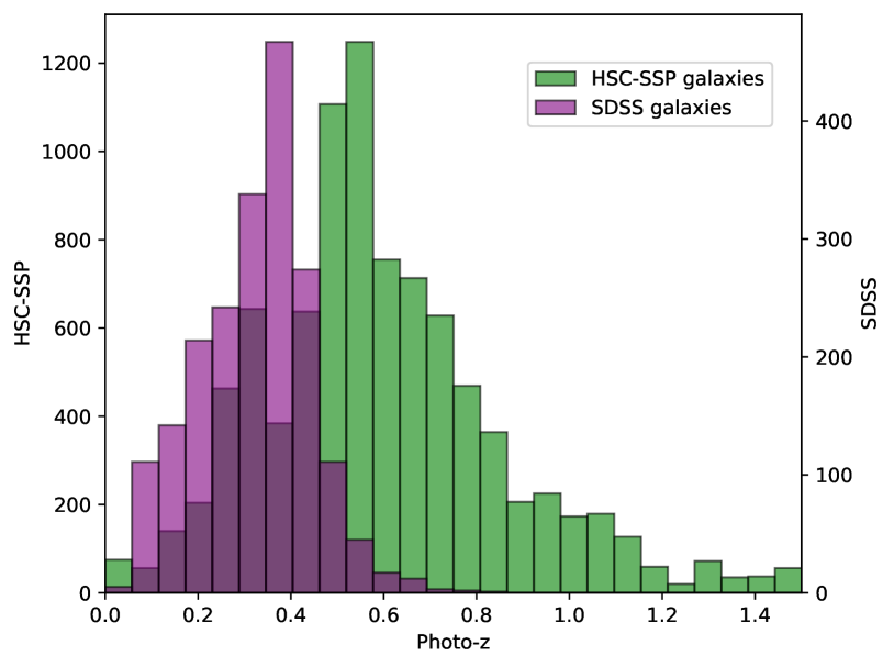
The goal of this paper is to develop an ML model that can accurately classify the objects detected by Pathfinder miniJPAS. As we will consider supervised ML algorithms, we need, for the learning process, a trustworthy classification by some other survey that has a sufficiently high overlap with miniJPAS. We use SDSS and HSC-SSP data, whose classification is expected to be trustworthy within the intervals $15\leq r\leq 20$ and $18.5\leq r\leq 23.5$, respectively. As said earlier, by “stars” we mean point-like objects that are not galaxies, that is, both stars and quasars. We assume that the classification by SDSS and HSC-SSP is trustworthy within this definition (Alam et al., 2015; Aihara et al., 2019).

We found 1810 common sources with SDSS, 691 galaxies and 1119 stars, and 11089 common sources with HSC-SSP, 9398 galaxies and 1691 stars. See Fig. 1 for the $r$-band distributions of stars and galaxies and Fig. 2 for the redshift distribution of galaxies.

2.1.1 SDSS classification

SDSS is a photometric and spectroscopic survey conducted at the Apache Point Observatory (New Mexico, USA) with a 2.5-m primary mirror. We used the SDSS DR12 photometric catalog minijpas.xmatch_sdss_dr12. Stars are defined according to an extendedness (difference between the CModel and PSF magnitudes) less than 0.145.

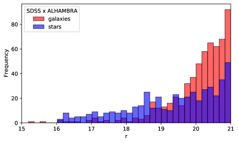
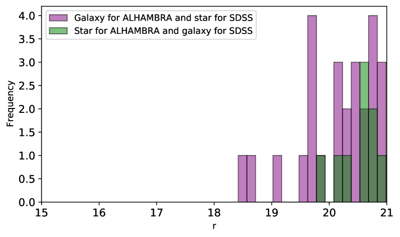
In order to test the photometric calibration by SDSS we crossmatched the latter with the catalog from the ALHAMBRA (Advance Large Homogeneous Area Medium Band Redshift Astronomical) survey (Moles et al., 2008). We obtained 1055 sources after imposing mask and saturation flags. As discussed in Molino et al. (2014), ALHAMBRA provides a trustworthy classification in the magnitude range $15\leq r\leq 21$.

As one can see from Fig. 3 (top) ALHAMBRA covers the relevant magnitude range and agrees with SDSS well till $r=20$ (bottom). Indeed, within $15\leq r\leq 20$, the percentages of false negatives and false positives are 0.2% and 1.9%, respectively (positive refers to the object being a galaxy). Note that, for the value added catalog, we will use SDSS in the more limited range $15\leq r\leq 18.5$ so that the percentages of false negatives and false positives are 0% and 0.7%, respectively (using $p_{\rm cut}=0.5$, see Section 4.1).

Figure 3: Top: Histograms of the $r$-band magnitudes of the objects resulting from the crossmatch between the SDSS catalog used in this paper and ALHAMBRA. Galaxies are shown in red, stars in semi-transparent blue. Bottom: disagreement between SDSS and ALHAMBRA as a function of $r$ magnitude. Sources classified as galaxies by ALHAMBRA and as stars by SDSS are in purple, while vice versa in semi-transparent green.

2.1.2 HSC-SSP classification

The HSC-SSP is a photometric survey with a 8.2-m primary mirror located in Hawaii, USA. We crossmatched the miniJPAS data with the wide field from the Public Data Release 2. Stars are defined according to an extendedness less than 0.015. We used the following data quality constraints: isprimary = True, r_extendedness_flag!=1 and r_inputcount_value>=4 for HSC-SSP, and flag=0 and mask=0 for miniJPAS. The crossmatch was performed with the TOPCAT software with a tolerance of 1 arcsec.

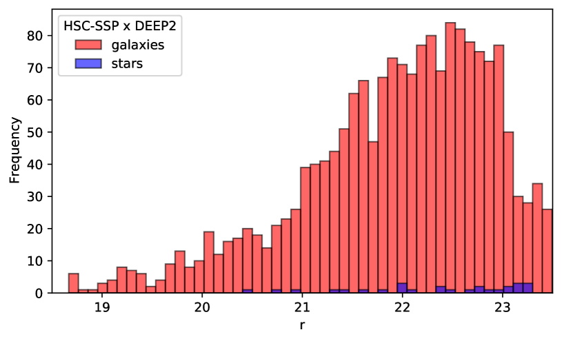
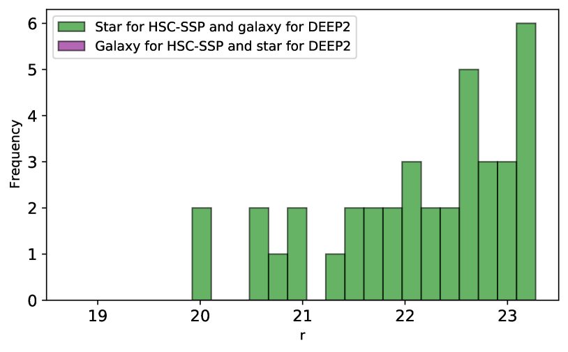
In order to test the photometric calibration by HSC-SSP we crossmatched the latter with the spectroscopic catalogs from the DEEP2 Galaxy Redshift Survey (1992 sources Matthews et al. (2013)). We could not use this spectroscopic catalog to check the photometric SDSS calibration because it does not cover the required magnitude range.

As one can see from Fig. 4 (top) DEEP2 covers the relevant magnitude range and agrees with HSC-SSP well (bottom). Indeed, for the range $18.5\leq r\leq 23.5$, the percentages of false negatives and false positives are 1.9% and 0%, respectively.

Figure 4: Top: Histograms of the $r$-band magnitudes of the objects resulting from the crossmatch between the HSC-SSP catalog used in this paper and DEEP2. Bottom: disagreement between HSC-SSP and DEEP2 as a function of $r$ magnitude. No object was classified as galaxy by HSC-SSP and star by DEEP2.

2.2 Input parameters for the ML algorithms

The features that are used as input for our algorithms can be grouped into photometric and morphological classes. Besides these two sets of features, we also consider the average PSF in the $r$ detection band of the 4 fields of miniJPAS, which is 0.70” for AEGIS1, 0.81” for AEGIS2, 0.68” for AEGIS3 and 0.82” for AEGIS4. The different PSF values signal different observing conditions: by including the PSF value we let the ML algorithms know that data is not homogeneous.

2.2.1 Photometric information

As photometric information we consider the MAG_AUTO magnitudes associated to the 60 filters together with their errors. The rationale behind including the errors is that, in this way, one can characterize the statistical distribution associated to a magnitude measurement. Indeed, observations may suffer from inhomogeneity due to varying observing conditions and the measurement errors should be able to account, at least in part, for this potential bias. As we will see, how well can one measure the magnitude associated to a filter may be more important than the actual measurement.

As said earlier, sources are detected in the $r$ band so that one may have non-detection in the other filters. Null or negative fluxes (after background subtraction) are assigned a magnitude value of 99. The ML algorithms are expected to learn that 99 marks missing values.

2.2.2 Morphological information

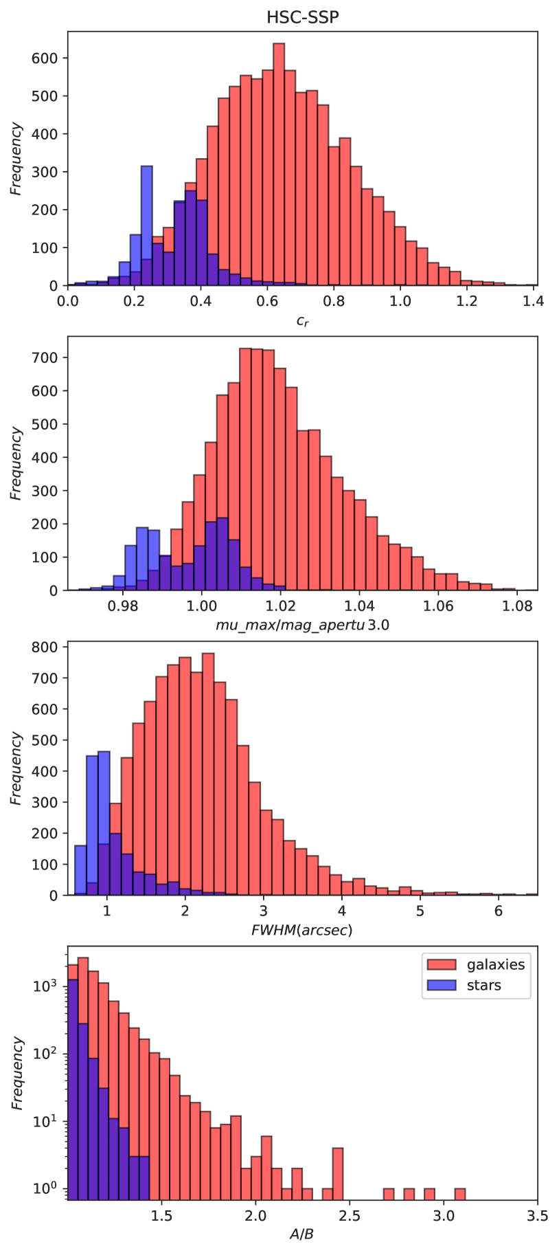
We consider the following 4 morphological parameters:

• concentration $c_{r}=r_{1.5^{\prime\prime}}-r_{3.0^{\prime\prime}}$, where $r_{1.5^{\prime\prime}}$ and $r_{3.0^{\prime\prime}}$ are the $r$-band magnitudes within fixed circular apertures of 1.5” and 3.0”, respectively,

• ellipticity $A/B$, where $A$ and $B$ are the RMS of the light distribution along the maximum and minimum dispersion directions, respectively.

• the full width at half maximum $FWHM$ assuming a Gaussian core,

• MU_MAX/MAG_APER_3_0 ($r$ band), where MU_MAX and MAG_APER_3_0 are the peak surface brightness above background and the magnitude within 3.0”, respectively. Note that here we are taking the ratio in order to have a parameter that is complementary to $c_{r}$.

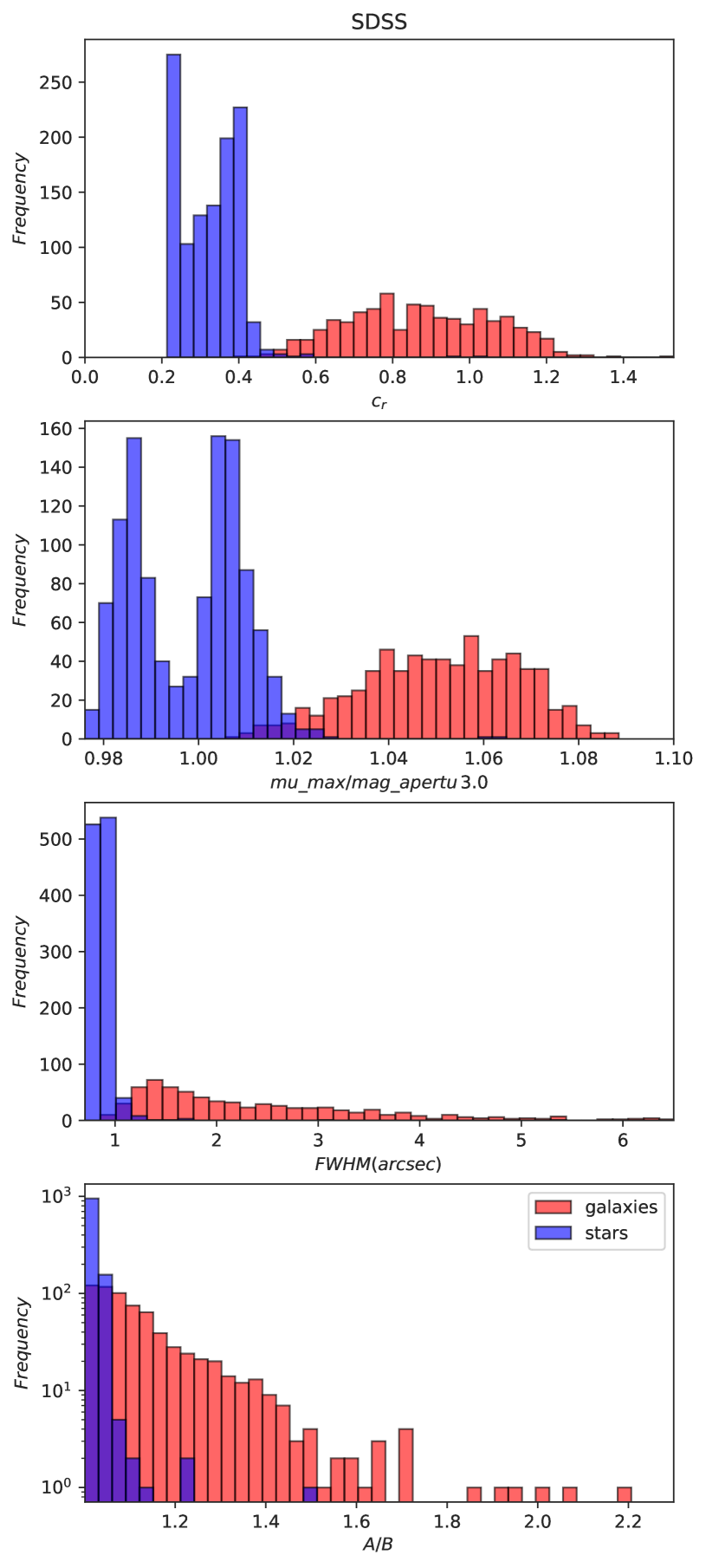
Figures 5 and 6 show their distributions for stars and galaxies and the two catalogs. The stellar bimodality in $c_{r}$ and MU_MAX/MAG_APER_3_0 is due to the fact that the four fields feature a different average PSF. We discuss these figures when examining feature importance in Section 5.4.

Figure 5: Distributions of the morphological parameters of stars and galaxies for the miniJPAS catalog crossmatched with SDSS. Galaxies are shown in red, stars in semi-transparent blue.

Figure 6: Distributions of the morphological parameters of stars and galaxies for the miniJPAS catalog crossmatched with HSC-SSP. Galaxies are shown in red, stars in semi-transparent blue.

2.3 J-PAS star/galaxy classifiers

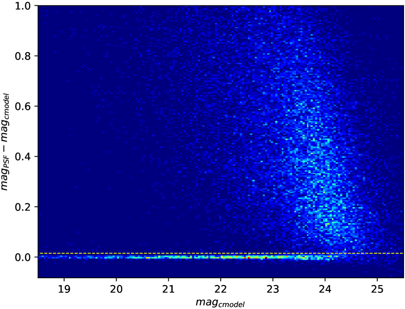
Here, we briefly discuss the star/galaxy classifiers available for miniJPAS. However, first we show how HSC-SSP classifies objects into stars and galaxies. This is performed by drawing a “hard cut” in the source parameter space. In Figure 7 we plot the difference between $mag_{PSF}$ and $mag_{cmodel}$ as a function of $mag_{cmodel}$ for the HSC-SSP data using their $r$ band (for the definitions see Aihara et al., 2019). Stars are expected to have $mag_{PSF}\simeq mag_{cmodel}$ while galaxies, due to their extended structure, should feature $mag_{PSF}>mag_{cmodel}$. Therefore, one can separate stars from galaxies via a cut in the extendedness parameter $mag_{PSF}-mag_{cmodel}$, which we show with a yellow line in Figure 7. The disadvantage of this model is that it provides an absolute classification for a scenario in which the uncertainties increase as we move toward weaker magnitudes. Note that for $r_{cmodel}\gtrsim 24$ the separation is not reliable as stars do not cluster anymore around a null extendedness.

Figure 7: Density of objects as a function of extendedness (the difference between $mag_{PSF}$ and $mag_{cmodel}$) and $mag_{cmodel}$ for HSC-SSP data. The yellow line marks an extendedness of 0.015. According to this morphological classification the sources below the cut are stars and the ones above the cut are galaxies.

2.3.1 CLASS_STAR

SExtractor (Source Extractor, Bertin & Arnouts, 1996) is a software developed for processing large images (60k $\times$ 60k pixels). It has been widely applied to photometric surveys including miniJPAS. Besides detecting sources, SExtractor also classifies objects into stars and galaxies. The software has two internal classifiers, CLASS_STAR and SPREAD_MODEL. miniJPAS includes the classification via CLASS_STAR which is based on neural networks (see Section 3.5). The network has 10 inputs: 8 isophotal areas, the peak intensity and the “seeing” control parameter. The output is probabilistic and quasars are classified as stars (in agreement with our convention). CLASS_STAR is reliable up to $r\sim 21$ (see also Bertin & Arnouts, 1996).

2.3.2 Stellar/galaxy loci classifier

miniJPAS includes the Bayesian classifier (SGLC) developed by López-Sanjuan et al. (2019) for J-PLUS data. The concentration versus magnitude diagram presents a bimodal distribution, corresponding to compact point-like objects and extended sources. López-Sanjuan et al. (2019) models both distributions to obtain the probability of each source to be compact or extended. The model with suitable priors is then used to estimate the Bayesian probability that a source is a star or a galaxy. Also in this case quasars are expected to be classified as “stars.” This method was updated to miniJPAS data, in particular a different galaxy population model was adopted. See Bonoli et al. (2020) for more details.

3 Machine learning

Machine learning is a branch of artificial intelligence that includes statistical and computational methods dedicated to providing predictions or taking decisions without being explicitly programmed to perform the task. Machine learning is employed in a variety of computing tasks, for which the explicit programming of well-performing algorithms is difficult or unfeasible. ML methods can either be supervised or unsupervised. The former learn from pre-classified data that has known inputs and outputs. When classification is unavailable, one relies instead on unsupervised methods, which can group items that are related in the parameter space, i.e., learn without the need of external information.

In this paper, we focus on binary supervised classification methods. In this case, the model (the internal parameters of the algorithm) is implicitly adjusted via the “training set.” Its performance is then tested with the remaining part of the dataset—the “test set.” Specifically, the internal parameters of the prediction function $f:\mathbb{R}^{n}\to Y$ are trained via the training dataset $\mathbf{x}_{i}\in\mathbb{R}^{n}$ ($n$ is the dimensionality of the feature space, $i$ labels the elements of the training set) with classifications $y_{i}$ $\in\{0,1\}$, where 1 stands for galaxy and 0 for star. Classifiers are divided into non-probabilistic and probabilistic classifiers. The former type of classifier outputs the best class while the latter the probability of the classes (the best class is taken as the one with the highest probability). Here, we will consider only binary probabilistic classifiers so that it is $f:\mathbb{R}^{n}\to[0,1]$, that is, $f$ gives the probability that an object is a galaxy. The probability of being a star is simply $1-f$. A value of $f$ close to 1 means that the object is likely a galaxy.

According to the No-Free Lunch theorem there is not an ideal algorithm that performs better than the others in any situation (Wolpert, 1996). As it is impossible to test all the methods available with all the possible choices of hyperparameters, we followed the strategy to explore firstly some of the main ML methods, namely, K-Nearest Neighbors (KNN), Decision Trees (DT), Random Forest (RF) and Artificial Neural Networks (ANN). Subsequently, because of the best response of the RF technique, we decide to focus on decision tree algorithms and ensemble models, so we added Extremely Randomized Trees (ERT) and Ensemble Classifier (EC) to our analysis. These algorithms can be used for both regression and classification. Here, we will only consider classification. We implemented these algorithms using the scikit-learn package written in python (Pedregosa et al., 2011). For more information about supervised learning see Mitchell (1997); Hastie et al. (2009). For the training and test sets we use 80% and 20% of the crossmatched catalogs, respectively. The division is performed randomly. This guarantees a good training and an accurate testing. A 70%-30% split is also a viable alternative. As mentioned in Section 2.1, the training sets are unbalanced as they feature a different number of galaxies and stars. We will show the purity curves for stars and galaxies in order to estimate the performance for each class. We now briefly review the six ML algorithms adopted in this paper. The hyperparameters used in the algorithms can be found in appendix F.

3.1 K-Nearest-Neighbors

The KNN algorithm is one of the most simple ML methods (Altman, 1992; Hastie et al., 2009). It calculates the distance between the element to be classified (within the test set) and the ones belonging to the training set. The predicted class will be calculated using the $k$ nearest neighbors. Although in this work we use the Euclidean metric, it is possible to choose others metrics to compute the distances. This method is very fast and its computational cost is proportional to the size of training set.

The output of the model is discrete if one uses the majority vote from the $k$ nearest neighbors. Here, we use the probabilistic version which assigns a probability to each class. In this case the classification is given by the average of the nearest $k$ neighbors:

$$f(\mathbf{x}_{q})=\frac{\sum_{i=1}^{k}w_{i}f(\mathbf{x}_{i})}{\sum_{i=1}^{k}w_{i}}\qquad\textrm{with}\qquad w_{i}=\frac{1}{d(\mathbf{x}_{q},\mathbf{x}_{i})^{2}}\,,$$ (1)

where the sum over the $k$ nearest neighbors is weighted by the weights $w_{i}$ which are the inverse of the square of the distance $d(\mathbf{x}_{q},\mathbf{x}_{i})$ from the neighbors ($\mathbf{x}_{i}$) to the element to be classified ($\mathbf{x}_{q}$, $q$ labels the test set), and $f(\mathbf{x}_{i})=y_{i}$ are the classifications of the training set. As discussed in Section 4.3, the number $k$ of neighbors is optimized via $k$-fold cross-validation. KNN has the advantage of being simple, intuitive and competitive in many areas. However, its computational complexity increases with the number of data.

3.2 Decision Trees

DT methods (see Breiman et al., 1984; Hastie et al., 2009) divide recurrently the parameter space according to a tree structure, following the choice of minimum class impurity of the groups at every split. To build a Decision Tree we first define an Information Gain (IG) function:

$$IG(D_{p},x_{t})=I(D_{p})-\frac{N_{\rm left}}{N_{p}}I(D_{\rm left})-\frac{N_{\rm right}}{N_{p}}I(D_{\rm right})\,,$$ (2)

where $D_{p}$ is the parent dataset of size $N_{p}$, $D_{\rm left}$ and $D_{\rm rigth}$ are the child datasets of sizes $N_{\rm left}$ and $N_{\rm right}$, respectively, and $I$ is a function called impurity. At every step the dataset is divided according to the feature and threshold $x_{t}$ that maximize the $IG$ function, or, equivalently, that minimize the impurity in the children dataset. We considered several impurity functions, such as entropy, classification error and Gini. For example, the latter is:

$$I_{G}(m)=1-\sum_{i=0,1}p(i|m)^{2}\,,$$ (3)

where $p(i|m)$ is the fraction of data belonging to the class $i$ (0 or 1) for a particular node $m$ that splits the parent dataset into the child datasets. After the growth of the tree is completed, the feature space is divided with probabilities associated to each class, and the probability for a test element is that of the region it belongs to.

During the branching process described above, some features appear more often than others. Using this frequency we can measure how important each feature is in the prediction process. We define the importance of each feature as:

$$Imp(x)=\sum_{t}\frac{N_{p}}{N_{\rm tot}}IG(D_{p},x_{t})\,,$$ (4)

where $N_{\rm tot}$ is the size of the dataset. The higher the number of times a feature branches a tree, higher its importance. Note that the first features that divide the tree tend to be of greater importance because the factor $N_{p}/N_{\rm tot}$ in Eq. (4) decreases as the tree grows ($N_{p}$ decreases). DT is characterized by an easy interpretability and handling but it is sensitive to small changes in the training set, thus suffering from potential biases.

3.3 Random Forest

Random Forest (Breiman, 2001; Hastie et al., 2009) is an ensemble algorithm built from a set of decision trees (the forest). Each tree generates a particular classification and the RF prediction is the combination of the different outputs. Each tree is different because of the stochastic method used to find the features when maximizing the IG function. Moreover, using the bootstrap statistical method, different datasets are built from the original one in order to grow more trees. For the discrete case the output is built from the majority vote, as seen with the KNN algorithm. For the probabilistic case we calculate the RF output as the average of the probabilities of each class for each tree. Finally, one computes the feature importances $Imp(x)$ for each tree of the ensemble and then averages them to obtain the RF feature importance. The diversity of trees decreases the bias as compared to DT, generating globally better models. On the other hand, RF requires greater memory and time as compared to DT.

3.4 Extremely Randomized Trees

Extremely Randomized Trees (Geurts et al., 2006) is an ensemble method similar to RF. There are only two differences between RF and ERT. The first is that ERT originally does not use bootstrap, although the implementation in scikit-learn allows one to insert it in the analysis. The second is that, while RF tries to find the best threshold for a features via the $IG$ function, in ERT the division is done randomly. Then, of all the randomly generated splits, the split that yields the highest score is chosen to split the node. For large datasets ERT algorithms are faster than RF ones and yield a similar performance (Geurts et al., 2006).

3.5 Artificial Neural Networks

Artificial Neural Networks mimic the functioning of the nervous system, being able to recognize patterns from a representative dataset (for an introduction see Mitchell, 1997; Hastie et al., 2009). The model we will use in our analysis consists of a simple supervised model called Multilayer Perceptron (MLP).

MLP consists of a set of perceptrons arranged in different layers. A perceptron, or artificial neuron, is a binary classifier. The data features are inserted in the input layer, the learning process occurs in the hidden layers, and the object classification is performed by the output layer. The information in the hidden layers is passed through each perceptron several times until convergence. In this algorithm, we can have several layers containing hundreds of perceptrons. To train the neural network, one uses a Cost Function that should be minimized. As learning method we use backpropagation (Rumelhart et al., 1986). We use LBFGS, Stochastic Gradient Descent and Adam cost functions, besides various activation functions. The values of the hyperparameters that give the best performance are given in Appendix F. In particular, we adopted 1 hidden layer with 200 neurons. ANN algorithms are very competitive and have the ability to deal with complex non-linear problems, but possess low interpretability and require powerful processors.

Finally, we briefly discuss the differences between CLASS_STAR and the ANN classifier used in this work. First, our ANN classifier is trained on real miniJPAS data, while CLASS_STAR was trained on simulated images. Second, although they both feature one hidden layer, CLASS_STAR has an input layer with 10 parameters and a hidden layer with 10 neurons while our classifier uses an input layer with 64 parameters (4 morphological features plus 60 photometric bands) and has a hidden layer with 200 neurons.

3.6 Ensemble Classifiers

The Ensemble method aims to construct a meta classifier from the union of different algorithms. Generally, when efficiently combined, these classifiers can perform better than the single best algorithm. In order to combine the classifiers we adopt the weighted sum rule with equal weights. The probability prediction function $f$ can be written as:

$$f(\textbf{x}_{q})=\frac{\sum^{m}_{j=1}w_{j}f_{j}(\textbf{x}_{q})}{\sum^{m}_{j=1}w_{j}}\,,$$ (5)

where $f_{j}(\textbf{x}_{q})$ is the probabilistic binary classification from the classifier $j$ and $m$ is the number of classifiers considered. We implemented this algorithm using the VotingClassifier function from scikit-learn. In the following, the ensemble classifier (EC) comprises ANN, RF and SGLC methods with equal weight ($w_{j}=1/3$). Note that EC is not a pure ML classifier as it uses SGLC, see Section 2.3.2. These algorithms generally will inherit the advantages and disadvantages of the methods which are based on.

4 Performance metrics

We will now introduce the metrics that we adopt in order to assess the performance of the classifiers. See Mitchell (1997); Hastie et al. (2009) for more details.

4.1 Confusion Matrix

As we are considering probabilistic classifiers, the classification of sources into stars or galaxies depends on a probability threshold $p_{\rm cut}$ to be specified. In our case, all objects with $f>p_{\rm cut}$ will be classified as galaxies. The choice of $p_{\rm cut}$ depends on completeness and purity requirements.

Once $p_{\rm cut}$ is specified, one can summarize the classification performance using the confusion matrix, which thoroughly compares predicted and true values. For a binary classifier the confusion matrix has four entries: True Positives (TP), True Negatives (TN), False Positives (FP) and False Negatives (FN). TP are sources correctly classified as galaxies by the model. TN are sources correctly classified as stars. FN are sources classified as stars by the model when, actually, they are galaxies. FP are sources classified as galaxies when they are stars.

4.2 Metrics

The receiver operating characteristic (ROC) curve represents a comprehensive way to summarize the performance of a classifier. It is a parametric plot of the true positive rate (TPR) and false positive rate (FPR) as a function of $p_{\rm cut}$:

$$TPR(p_{\rm cut})=\frac{TP}{TP+FN}\qquad FPR(p_{\rm cut})=\frac{FP}{FP+TN}$$ (6)

with $0\leq p_{\rm cut}\leq 1$. TPR is also called “recall” and, in astronomy, is the completeness. The performance of a classifier can then be summarized with the area under the curve (AUC). The AUC can assume values between 0 and 1. A perfect classifier has a value of 1, while a random classifier, on average, a value of 1/2.

The purity curve is a useful method to assess the performance of an unbalanced classifier (as the training set does not feature the same number of stars and galaxies). It is a parametric plot of the completeness (or recall) and the purity (or precision) as a function of $p_{\rm cut}$:

$$\text{Purity}=\frac{TP}{TP+FP}\,.$$ (7)

In order to summarize the purity curve, we consider the average precision (AP) which is the area under the purity curve and takes values between 0 and 1.

Finally, one can measure the algorithm performance with the mean squared error ($MS\!E$) defined as:

$$MS\!E=\frac{1}{N_{\rm test}}\sum_{q=1}^{N_{\rm test}}\left(y_{q}-f(\mathbf{x}_{q})\right)^{2}\,,$$ (8)

where $y_{q}$ are the test-set classifications and $N_{\rm test}$ is the test-set size. $MS\!E=0$ characterizes a perfect performance. In the present case of a binary classifier it is $MS\!E=(FP+FN)/N_{\rm test}$.

4.3 $k$-fold cross-validation

We use the $k$-fold cross-validation method in order to optimize the algorithm’s hyperparameters, test for overfitting and underfitting and estimate the errors on AUC and AP. $k$-fold cross-validation separates the training data in $k$ equal and mutually exclusive parts (we adopt $k=10$). The model is trained in $k-1$ parts and validated in the remaining one, called validation. This process is repeated cyclically $k$ times. The final result is the mean and standard deviation of the metric.

The ML methods described in Section 3 depend on several internal hyperparameters (for example, the number $k$ of neighbors in KNN). In order to optimize them we performed $k$-fold cross-validation for several hyperparameter configurations. The results of the next Section are relative to the best configuration according to the AUC. See Appendix F for details.

We also tested the ML algorithms against overfitting and underfitting. The former happens when the training is successful (high AUC) but not the testing (low AUC). The latter when training and testing are not successful (both AUC’s are low). We checked that the average AUC from the $k$-fold cross-validation agrees with the AUC from the test set; all the methods pass this test.

Finally, we can use $k$-fold cross-validation in order to estimate the error in the determination of the AUC and AP. This will help us understand if the differences between two estimators are significative and also how sensitive a classifier is with respect to the division of the dataset into training and test sets.

5 Results

Table 1: Performance of the classifiers considered in this paper for the miniJPAS catalog crossmatched with the SDSS catalog ($15\leq r\leq 20$, top) and with the HSC-SSP catalog ($18.5\leq r\leq 23.5$, bottom). The best performance is marked in bold (EC is not considered). $P$ stands for the analysis that uses only photometric bands while $M\!+\!P$ stands for the analysis that uses photometric bands together with morphological parameters.

miniJPAS-SDSS	$AUC_{M+P}$	$AUC_{P}$	$AP_{M+P}^{\rm gal}$	$AP_{P}^{\rm gal}$	$MS\!E_{M+P}$	$MS\!E_{P}$
SGLC	0.994	–	0.989	–	0.006	–
CLASS_STAR	0.997	–	0.993	–	0.032	–
KNN	$0.996\!\pm\!0.003$	$0.991\!\pm\!0.007$	$0.990\!\pm\!0.008$	$0.984\!\pm\!0.009$	0.015	0.027
DT	$0.992\!\pm\!0.006$	$0.984\!\pm\!0.012$	$0.983\!\pm\!0.011$	$0.974\!\pm\!0.018$	0.011	0.032
RF	$\mathbf{0.997\!\pm\!0.006}$	$0.996\!\pm\!0.004$	$0.992\!\pm\!0.009$	$0.995\!\pm\!0.010$	0.006	0.019
EC	0.997	0.997	0.995	0.996	0.006	0.014
ANN	$0.997\!\pm\!0.004$	${0.988\!\pm\!0.009}$	$\mathbf{0.994\!\pm\!0.017}$	$0.983\!\pm\!0.015$	0.012	0.043
ERT	$0.997\!\pm\!0.002$	$\mathbf{0.997\!\pm\!0.003}$	$0.993\!\pm\!0.006$	$\mathbf{0.996\!\pm\!0.004}$	0.005	0.019
miniJPAS-HSC-SSP	$AUC_{M+P}$	$AUC_{P}$	$AP_{M+P}^{\rm gal}$	$AP_{P}^{\rm gal}$	$MS\!E_{M+P}$	$MS\!E_{P}$
SGLC	0.970	–	0.992	–	0.040	–
CLASS_STAR	0.956	–	0.991	–	0.053	–
KNN	$0.950\!\pm\!0.010$	$0.824\!\pm\!0.023$	$0.989\!\pm\!0.003$	$0.959\!\pm\!0.006$	0.053	0.098
DT	$0.961\!\pm\!0.009$	$0.855\!\pm\!0.017$	$0.990\!\pm\!0.003$	$0.959\!\pm\!0.007$	0.061	0.132
RF	$0.978\!\pm\!0.005$	$\mathbf{0.938\!\pm\!0.007}$	$0.995\!\pm\!0.002$	$\mathbf{0.986\!\pm\!0.002}$	0.032	0.054
EC	0.979	0.967	0.996	0.993	0.031	0.040
ANN	$0.970\!\pm\!0.007$	$0.885\!\pm\!0.014$	$0.993\!\pm\!0.003$	$0.969\!\pm\!0.005$	0.036	0.070
ERT	$\mathbf{0.979\!\pm\!0.006}$	$0.931\!\pm\!0.006$	$\mathbf{0.995\!\pm\!0.002}$	$0.982\!\pm\!0.002$	0.032	0.053

We now present our results for the algorithms introduced in Sections 3 applied to the crossmatched catalogs described in Section 2.1. Regarding stars and galaxy number counts we refer the reader to the miniJPAS presentation paper (Bonoli et al., 2020).

5.1 miniJPAS-SDSS catalog

The performance of the star/galaxy classifiers considered in this paper for the miniJPAS catalog crossmatched with the SDSS catalog in the magnitude interval $15\leq r\leq 20$ is excellent. The results are summarized in Table 1, where the best result are marked in bold (EC is not considered as it is not a pure ML classifier). The errors on the pure-ML classifiers are estimated via $k$-fold cross-validation. In order to assess the importance of photometric bands and morphological parameters, the analysis considers two cases: only photometric bands ($P$ subscript in the table) and photometric bands together with morphological parameters ($M+P$ subscript in the table). Note that this distinction does not apply to SGLC and CLASS_STAR as they always include the use of morphological parameters.

Regarding the analysis with photometric bands only, the best ML methods are RF and ERT, showing the power of combining several trees when making a prediction. Remarkably, using only photometric information, RF and ERT outperform SGLC and CLASS_STAR. If now we add morphological information, the almost perfect performance of RF and ERT does not improve, showing again that, in this magnitude range, photometric information is sufficient. In Table 1 we also show the $MS\!E$, whose results agree with the ones from the ROC and purity curves.

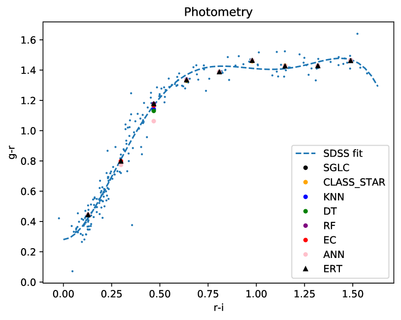
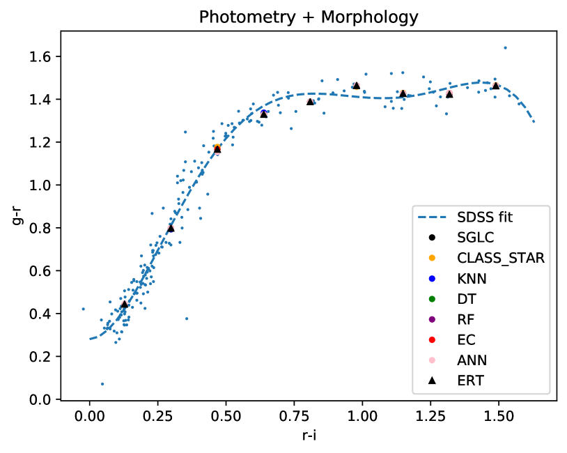
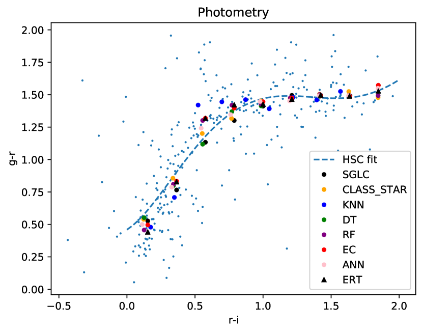
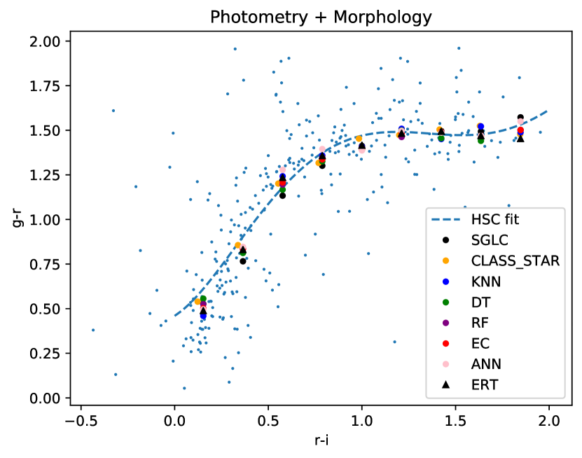
Another way to analyze qualitatively the performance of a classifier is via a color-color diagram for objects classified as stars ($p\leq p_{\rm cut}=0.5$). Figure 8 shows the stellar locus in the $g-r$ versus $r-i$ color space. The blue line is a fifth-degree polynomial fit, based on miniJPAS data that were classified as stars by SDSS. The various markers represent the averages of each classifier for different bins. We observe a small dispersion around the curve, which decreases when morphological parameters are included. This indicates that the classifiers and the classification from SDSS are in good agreement.

Figure 8: The blue small dots represent the stellar locus for the objects classified as stars ($p\leq p_{\rm cut}=0.5$) of the miniJPAS catalog crossmatched with the SDSS catalog in the magnitude interval $15\leq r\leq 20$. The dashed line represent a polynomial fit to the stellar locus. The top panel is relative to the analysis that uses only photometric bands, while the bottom panel is relative to the analysis that also uses morphological information. The colored larger symbols represent the mean stellar locus provided by the different ML models. For comparison it is shown also the classification by CLASS_STAR and SGLC that always use morphological parameters.

5.2 miniJPAS-HSC-SSP catalog

Figure 9: ROC curves (left panels) and purity curves for galaxies (right panels) for the classifiers considered in this paper for the miniJPAS catalog crossmatched with the HSC-SSP catalog in the magnitude interval $18.5\leq r\leq 23.5$. The top panels are relative to the analysis that uses only photometric bands while the bottom panels to the analysis that uses photometric bands and morphological parameters. For comparison it is shown also the classification by CLASS_STAR and SGLC that always use morphological parameters. Note that the axes ranges are varied in order to better show the curves. The results are summarized in Table 1 (bottom).

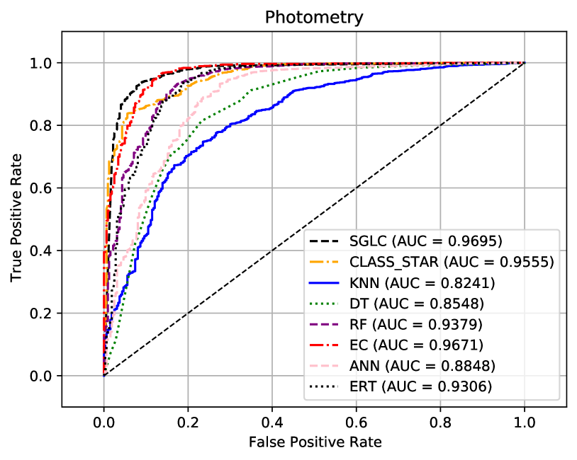
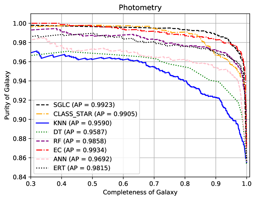
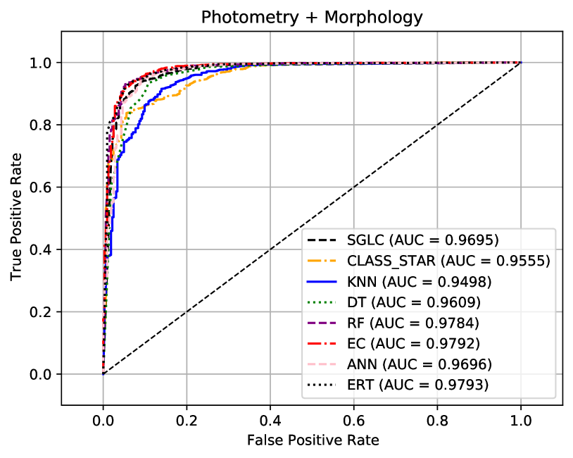
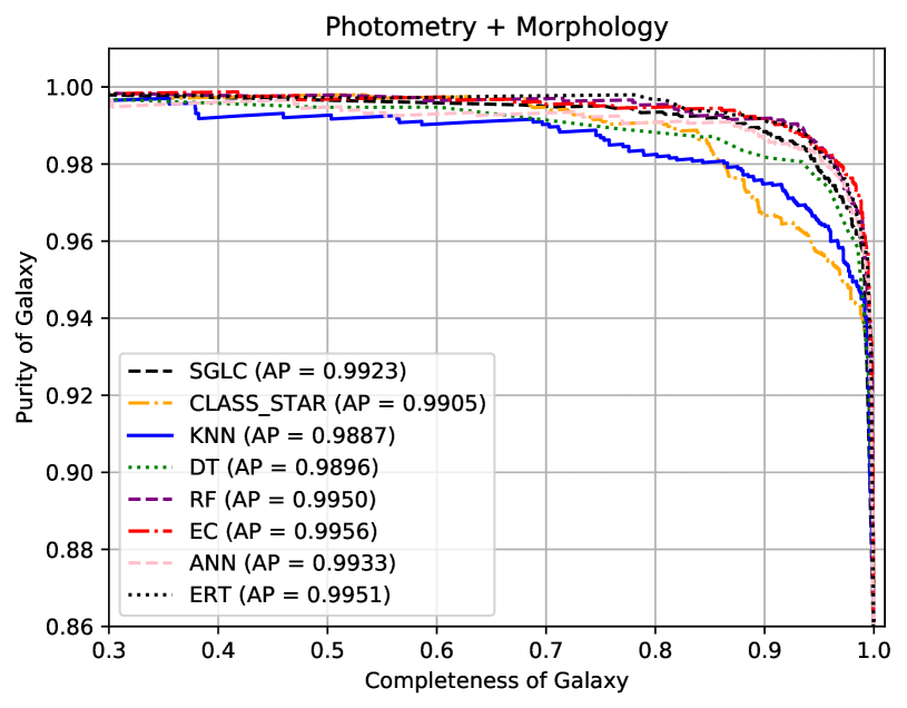
As shown in the previous Section, star/galaxy classification in the range $15\leq r\leq 20$ is not problematic. However, the scenario changes when one moves to fainter magnitudes. As the amount of light decreases, with less information reaching the telescope, the performance of the algorithms decreases to the point that it is important to look for alternative solutions such as ML. Here, we present the analysis of the previous Section applied to the miniJPAS catalog crossmatched with the HSC-SSP catalog in the magnitude interval $18.5\leq r\leq 23.5$.

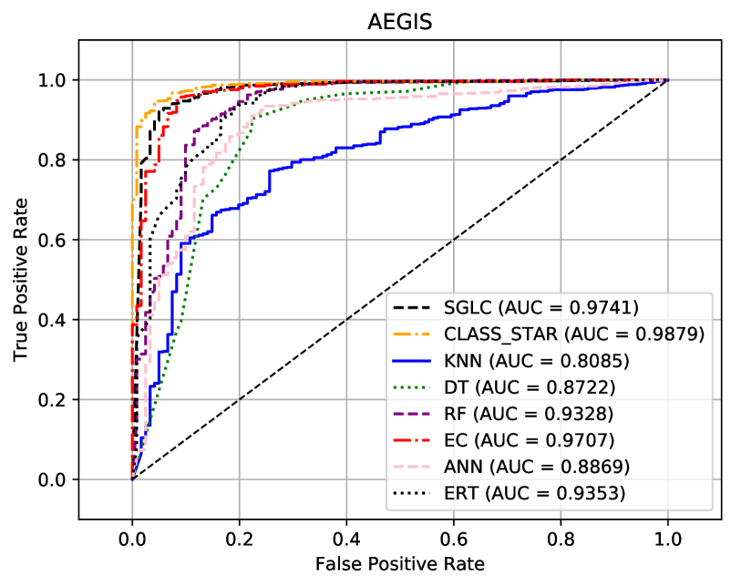
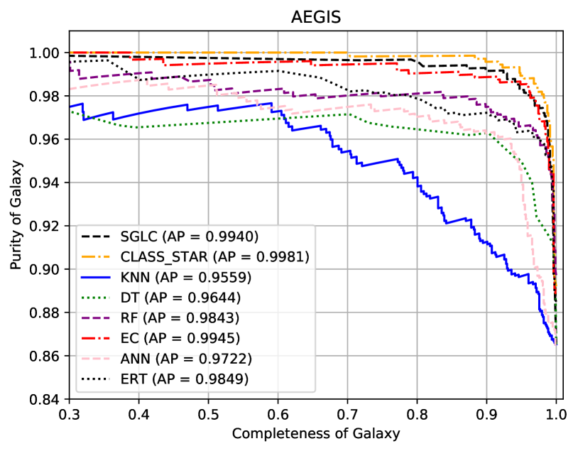
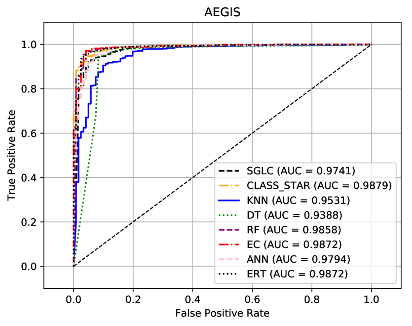
Figure 9 and Table 1 show the results. Using photometric information only, the RF algorithm achieves the remarkable score of $AUC=0.938$. Although it is less performant than SGLC and CLASS_STAR (that use morphology), this result shows that ML has the potential of identifying compact galaxies, which share the same morphology of stars. Also, it has been argued that models that use just photometry can classify QSO’s as extragalactic objects better than models that use morphological parameters (Costa-Duarte et al., 2019). The use of the morphological parameters improves the performance of the ML methods to the point that ERT and RF perform better than CLASS_STAR and SGLC. In Appendix C we repeat the analysis of Figure 9 for the mJP-AEGIS1 field, which is the miniJPAS pointing with the best point spread function (PSF).

It is interesting to note that, although the classifiers feature lower $AUC$’s and higher $MS\!E$’s as compared to the analyses of the previous Section, the $AP$’s reach similar values, even when we use only photometric bands. This is due to this dataset having many more galaxies and only 15.3% of stars. Therefore, even if there are contaminations by stars, the impact is lower.

Finally, in Figure 10 we show the stellar locus. We can observe a greater dispersion as compared with Figure 8, especially when we use only photometric bands in the analysis. Nevertheless, the ML methods return the correct shape of the stellar locus and their performance is similar to the one by SGLC.

Figure 10: The blue small dots represent the stellar locus for the objects classified as stars ($p\leq p_{\rm cut}=0.5$) of the miniJPAS catalog crossmatched with the HSC-SSP catalog in the magnitude interval $18.5\leq r\leq 23.5$. The dashed line represent a polynomial fit to the stellar locus. The top panel is relative to the analysis that uses only photometric bands, while the bottom panel is relative to the analysis that also uses morphological information. The colored larger symbols represent the mean stellar locus provided by the different ML models. For comparison it is shown also the classification by CLASS_STAR and SGLC that always use morphological parameters.

5.3 Value added catalog

The ultimate goal of this work is to release a value added catalog with our best alternative classification. In the previous Section we studied star/galaxy classification in the (partially overlapping) magnitude ranges $15\leq r\leq 20$ and $18.5\leq r\leq 23.5$. Here, in order to have a uniform dependence on $p_{\rm cut}$, we wish to produce a catalog that is obtained using a single classifier. As seen in Section 2.1, in the magnitude range $18.5\leq r\leq 20$, the classification by HSC-SSP is more reliable than the one by SDSS. Therefore, we consider the classification by SDSS in the range $15\leq r<18.5$ and the one by HSC-SSP in the range $18.5\leq r\leq 23.5$. This catalog spans the magnitude range $15\leq r\leq 23.5$ and features a total of 11763 sources, 9517 galaxies and 2246 stars. We call it XMATCH catalog.

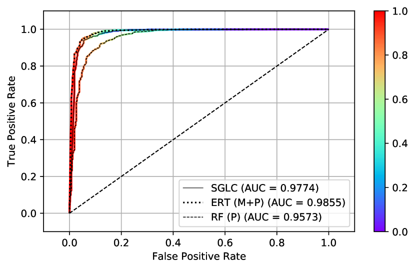
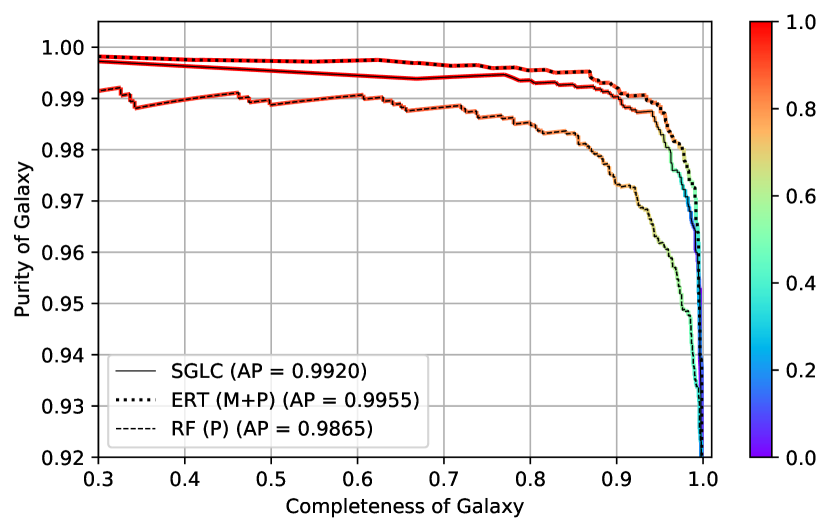
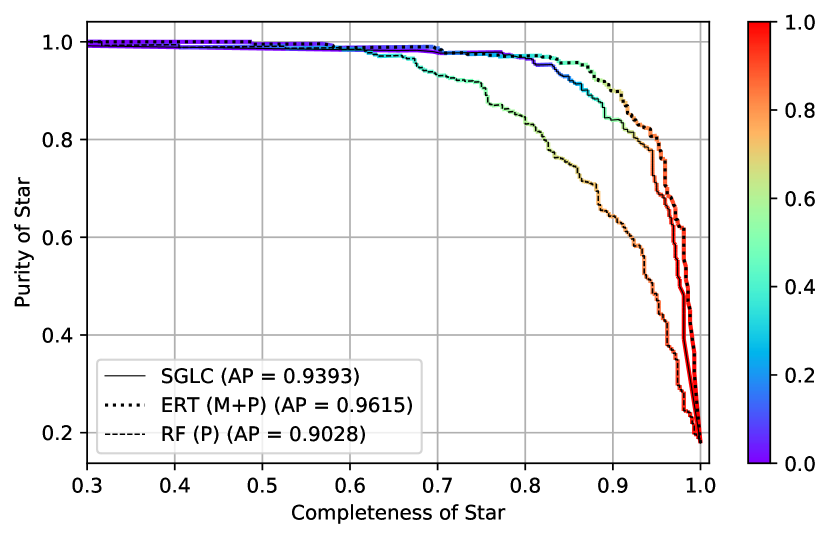
Next, we train and test all the models on this catalog. Using only photometric information the best classifier is RF, which reaches $AUC=0.957\pm 0.008$, close to the performance of SGLC that uses morphological information. Using photometric and morphological information the best classifier is ERT, which, with $AUC=0.986\pm 0.005$, outperforms SGLC. Figure 11 shows the ROC curve and the purity curve for galaxies and stars for the three classifiers above, with the addition of the probability threshold $p_{\rm cut}$ via color coding. These plots are meant to help choosing the probability threshold that best satisfies one’s needs of completeness and purity (see also Appendix B). These plots were made with the code available at github.com/PedroBaqui/minijpas-astroclass. As shown in the bottom panel of Figure 11, the AP of stars is quite good (and significantly better than SGLC), showing that the fact that we used an unbalanced set did not affect the results regarding the least represented class.

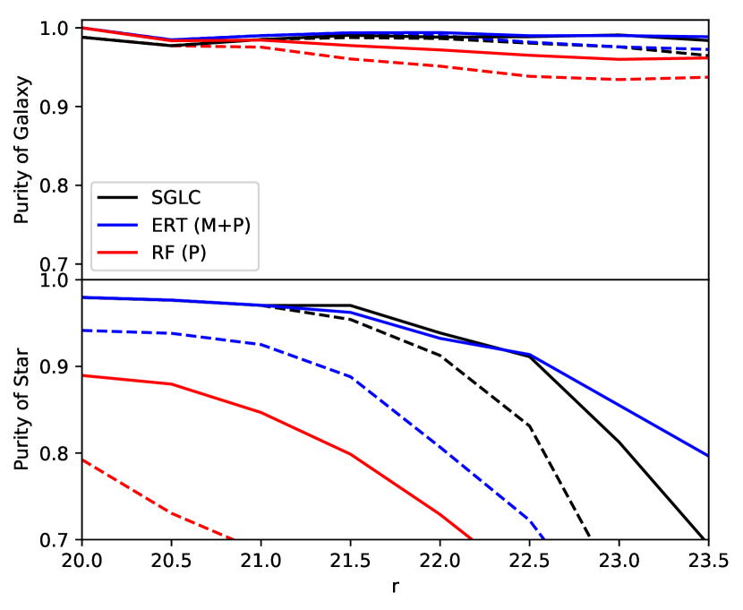
Finally, we show in Figure 12 the cumulative purity of the galaxy and star samples as a function of $r$ magnitude for a fixed completeness of 95% and 99%, which are achieved by choosing a suitable $p_{\rm cut}$. For a completeness of 95% and the ERT classifier, the purity of the galaxy sample remains higher than 99% throughout the magnitude range, better than SGLC. Regarding stars, for a completeness of 95% and ERT, purity remains higher that 90% for $r<22.5$. For fainter stars, ERT outperforms SGLC.

In order to build our catalog, we applied our two best classifiers (RF without morphology and ERT with morphology) to the 29551 miniJPAS sources in the magnitude range $15\leq r\leq 23.5$. It is important to note that, given the completeness of miniJPAS (see Bonoli et al., 2020), sources outside this magnitude interval are less likely to enter scientific studies. The catalog is publicly available at j-pas.org/datareleases via the ADQL table minijpas.StarGalClass. See Appendix D for more informations and an ADQL query example.

Figure 11: ROC curve (top panel) and purity curve for galaxies (middle panel) and stars (bottom panel) for RF (no morphology), ERT (with morphology) and SGLC for sources in the magnitude range $15\leq r\leq 23.5$. The color coding indicates the probability threshold $p_{\rm cut}$. Note that the axes ranges are varied in order to better show the curves.

Figure 12: Cumulative purity of the galaxy (top) and star (bottom) samples as a function of magnitude for the ML classifiers of Fig. 11, for a fixed completeness of 95% (solid line) and 99% (dashed line).

5.4 Feature importance

We use the RF algorithm (see Eq. 4) to assess feature importance which can give us insights on the way objects are classified. The 15 most important features are listed in Table 2. The full tables are provided as machine readable supplementary material.

When including morphological parameters, FWHM is the most important feature. This agrees with the distributions of FWHM in Figs. 5 and 6 which show a good separation between stars and galaxies. Although this separation is less evident for the other parameters, they also contribute to classification. In particular, the mean PSF is the fourth most importante feature, while the least important morphological feature is the ellipticity parameter $A/B$. To some extent, these results could depend on the choice of the impurity function (see Eq. (3)). We tested different impurity functions and confirmed that morphological parameters are generally more important than photometric bands.

When using photometric information only, the importance of the features is more evenly distributed as more features work together towards object classification. In particular, broad bands are not necessarily more important than narrow bands and errors (the width of the distribution) are as important as the measurements (central value of the distribution). In other words, the full characterization of the measurement seems to be important.

Figure 13: Top: The shaded area represents the relative importance (see Eq. 4) of the narrow-band filters as function of the filters’ wavelength for the analysis relative to the full magnitude range $15\leq r\leq 23.5$ (see Section 5.3). The importance of the 4 broad-band filters is shown using black circles. The red and blue lines show the average photo-spectrum of stars and galaxies, respectively. Bottom: as the top panels but for the relative importance of the magnitude errors. The green line shows the percentage of missing values (magnitude of 99) for the narrow band filters.

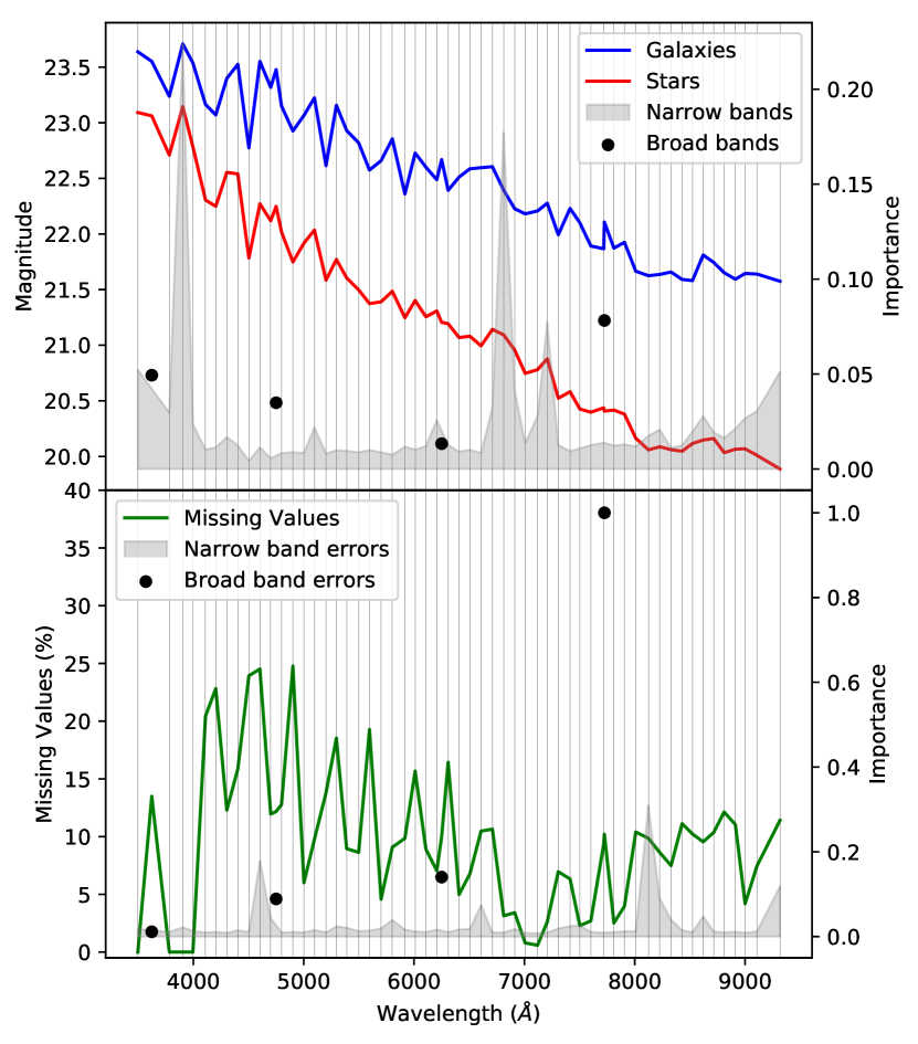
In order to get a physical insight on the regions of the spectrum that matter most for classification, we show in Figure 13 (top) the relative importance of the filters’s magnitudes as function of the filters’ wavelength together with the median star and galaxy photo-spectrum. It is clear that there are regions systematically more important than others (neighboring filters with higher importance) and that there is correlation between the most important regions and the average features in the spectra. In the bottom panel of Figure 13 we show the importance of the magnitude errors, which also show regions that are systematically more important than others. Particularly important is the error on the $i$ band. In the same panel we also show the fraction of missing values (magnitude of 99) for each narrow band filter. We can see that this fraction anti-correlates with the filter importance (top panel).

Table 2: Feature importance with ($M+P$) and without ($P$) morphological parameters for the analysis relative to the full crossmatched catalog XMATCH ($15\leq r\leq 23.5$, see Section 5.3). The importance is normalized relative to the best feature. The quantity max/ap3 is MU_MAX/MAG_APER_3_0. The full tables are provided as machine readable supplementary material. See also Figure 13.

XMATCH ($P$)		XMATCH ($P+M$)
Feature	Importance	Feature	Importance
iSDSSerr	1.00	FWHM	1.00
J0810err	0.31	$c_{r}$	0.30
J0390	0.22	max/ap3	0.18
J0460err	0.18	PSF	0.10
J0680	0.18	iSDSSerr	0.08
rSDSSerr	0.14	J0820err	0.02
J1007err	0.12	J0390err	0.02
J0820err	0.09	A/B	0.01
gSDSSerr	0.09	J1007err	0.01
iSDSS	0.08	J0810err	0.01
J0720	0.08	J0390	0.01
J0660err	0.07	gSDSS	0.009
uJAVA	0.05	uJAVAerr	0.008
J1007	0.05	J0790err	0.008
uJPAS	0.05	J0680	0.007
…	…	…	…

5.5 Transmission curve variability

The transmission curves of the narrow band filters vary according to the relative position in the filters. In particular, the transmission curve variability depends on the SED of each object so that the map of relative variation in flux for a given filter is different for objects with different SEDs. This effect should affect classifications that depend strongly on particular narrow spectral features (even more if they fall in one of the edges of the narrow band transmission curve) and would have almost no effect when considering mainly the continuum. As we use photometric data, our results could be impacted by this effect.

miniJPAS data, in particular the size of the XMATCH catalog, does not allow us to perform a thorough investigation of this effect. Therefore, we explore this issue by dividing the test set into the 4 quadrants of the filter area and compute the $AUC$ for each quadrant. The filter coordinates are given in pixels via the X_IMAGE and Y_IMAGE variables ($9000\times 9000$ pixels). As can be seen from Table 3, the $AUC$ variation is compatible with the overall performance of $AUC=0.957\pm 0.008$ (RF) and $AUC=0.986\pm 0.005$ (ERT), showing that the effect should not strongly bias our results.

Table 3: Area under the curve ($AUC$) for the 4 filter quadrants relative to the best classifiers shown in Figure 11.

RF ($P$)	$\texttt{X}<4500$	$4500\leq\texttt{X}\leq 9000$
$\texttt{Y}<4500$	0.9633	0.9592
$4500\leq\texttt{Y}\leq 9000$	0.9449	0.9588
ERT ($P+M$)	$\texttt{X}<4500$	$4500\leq\texttt{X}\leq 9000$
$\texttt{Y}<4500$	0.9917	0.9775
$4500\leq\texttt{Y}\leq 9000$	0.9822	0.9938

6 Conclusions

In this work we applied different machine learning methods for the classification of sources of miniJPAS. The goal was to build models that are competitive with and complementary to those adopted in the miniJPAS 2019 public data release and to offer to the astronomical community a value added catalog with an alternative classification. As we considered supervised ML algorithms, we classified the miniJPAS objects that are in common with SDSS and HSC-SSP, whose classifications are trustworthy within the magnitude intervals $15\leq r\leq 20$ and $18.5\leq r\leq 23.5$, respectively. We used as input the magnitudes associated to the 60 filters along with their errors, 4 morphological parameters and the mean PSF of the pointings. The output of the algorithms is probabilistic. We tested K-Nearest Neighbors, Decision Trees, Random Forest, Artificial Neural Networks, Extremely Randomized Trees and Ensemble Classifier.

Our results show that ML is able to classify objects into stars and galaxies without the use of morphological parameters. This makes ML classifiers quite valuable as they can distinguish compact galaxies from stars, differently from methods that necessarily use morphological parameters in the classification process. Of course, the inclusion of morphological parameters improves the results to the point that ERT can outperform CLASS_STAR and SGLC (the default classifier in J-PAS).

We used the RF algorithm to assess feature importance. When using morphological parameters, FWHM is the most important feature. When using photometric information only, we observe that broad bands are not necessarily more important than narrow bands and errors (the width of the distribution) are as important as the measurements (central value of the distribution). In other words, the full characterization of the measurement seems to be important. We have also shown that ML can give meaningful insights on the regions of the spectrum that matter most for classification.

After having validated our methods, we applied our best classifiers, with and without morphology, to the full dataset. This classification is available as a value added catalog at j-pas.org/datareleases via the ADQL table minijpas.StarGalClass. The ML models are available at github.com/J-PAS-collaboration/StarGalClass-MachineLearning. Our catalog both validates the quality of SGLC and produces an independent classification that can be useful to test the robustness of subsequent scientific analyses. In particular, our classification uses the full photometric information, with and without morphology, which is important for faint galaxies whose morphology is similar to the one of stars.

We conclude stressing that our methodology can be further improved both at the algorithmic and at the data input level. A promising avenue is the direct use of the object images with convolutional neural networks. This approach has the potential of outperforming presently available classifiers.

Appendix A Purity curves for stars

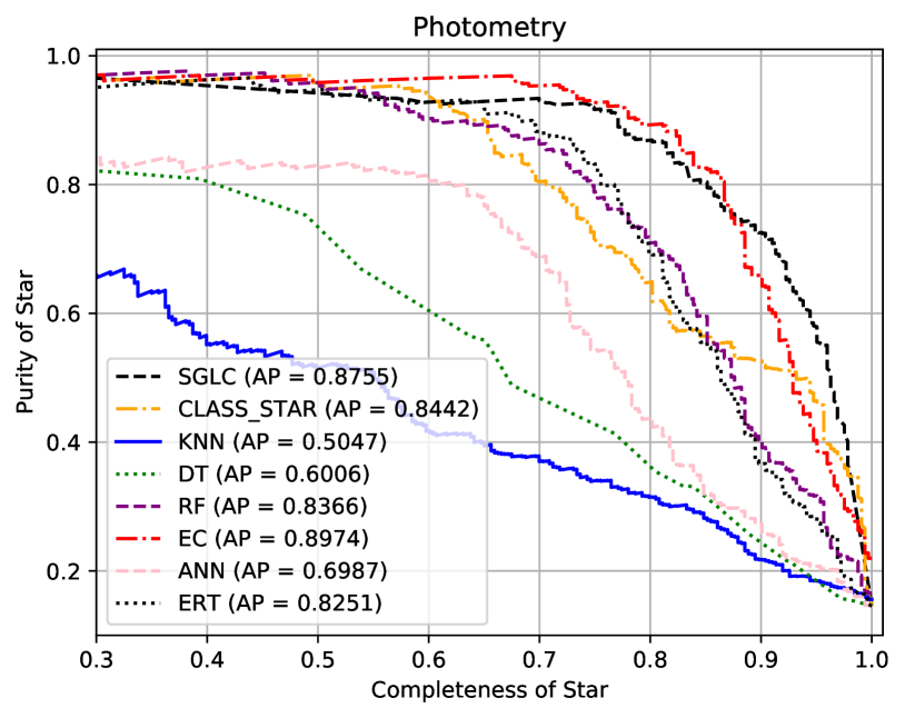
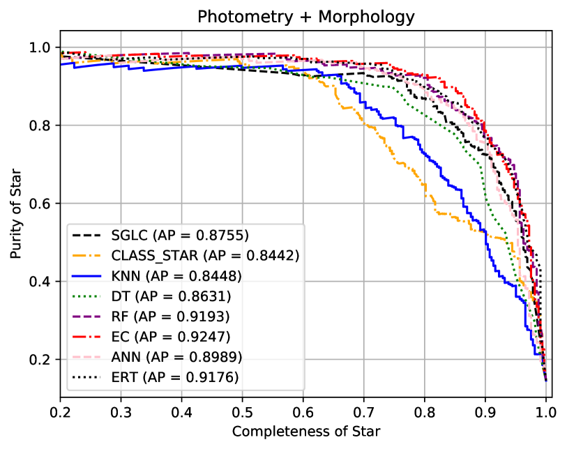
For completeness we report in Figure 14 the purity curves relative to the stars. For a comparison see, for example, Sevilla-Noarbe et al. (2018); Fadely et al. (2012); Cabayol et al. (2019).

Figure 14: Purity curves for stars using J-PAS data with HSC-SSP classification. The top panel uses only photometric information while the bottom one uses also morphology. For comparison it is shown the classification by CLASS_STAR and SGLC that always use morphological parameters. Note that the axes ranges are varied in order to better show the curves.

Appendix B Classification vs. probability threshold

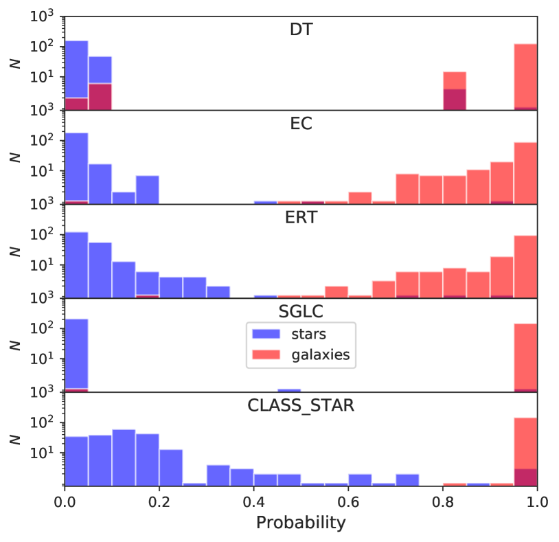
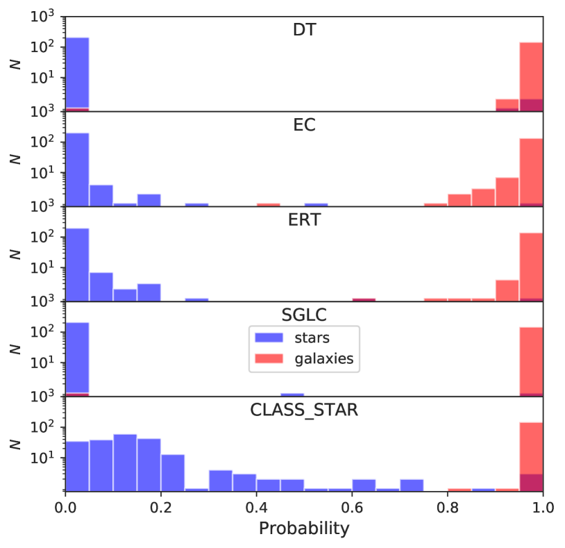
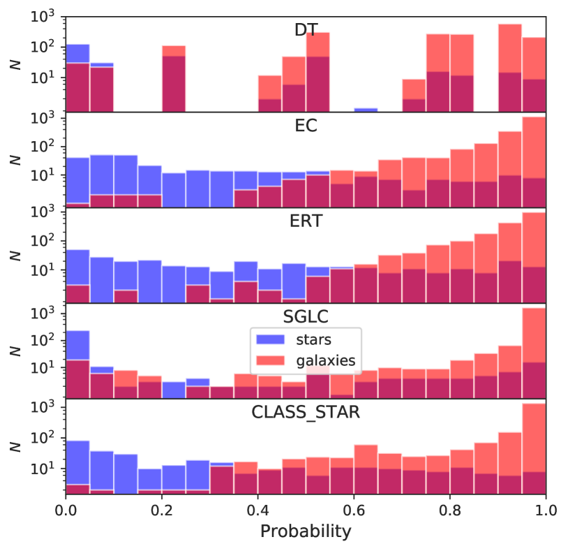
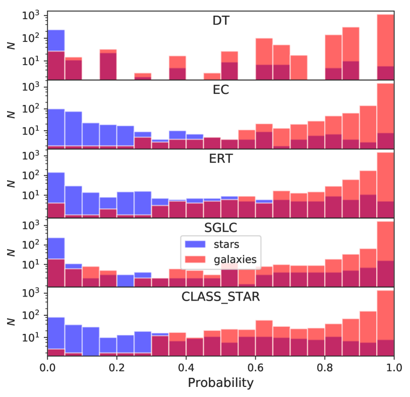
We show in Figure 15 the histograms of the probabilities that the objects received from the classifiers. In red we have objects classified as galaxies and in blue as stars. These plots allow us to assess the performance of the algorithms from a different point of view. When one choses a value for $p_{\rm cut}$, all the objects to the right of this value will be classified as galaxies while the ones with lower probability will be classified as stars. It is then clear that an ideal algorithm should have well separated and non-intersecting probability distributions for stars and galaxies.

A first remark is that the addition of morphology makes the distributions tighter and with less intersections. Similar results were obtained with CFHTLenS data (Kim et al., 2015) . We observe instead that the probability distribution of galaxies for CLASS_STAR is more concentrated than the probability distribution for stars. This leads us to the conclusion that CLASS_STAR has a tendency to classify galaxies better than stars. It is also clear that by varying $p_{\rm cut}$ one can sacrifice the completeness of the dataset in favor of a higher purity of galaxies.

Figure 15: Histograms of the probability that a source belongs to the class of galaxy. The histograms relative to actual stars and galaxies, as classified by SDSS (top) and HSC-SSP (bottom), are in blue and semi-transparent red, respectively. The panels on the left use only photometric information while the ones on the right use also morphology. For comparison it is shown also the classification by CLASS_STAR and SGLC that always use morphological parameters.

Appendix C mJP-AEGIS1 field

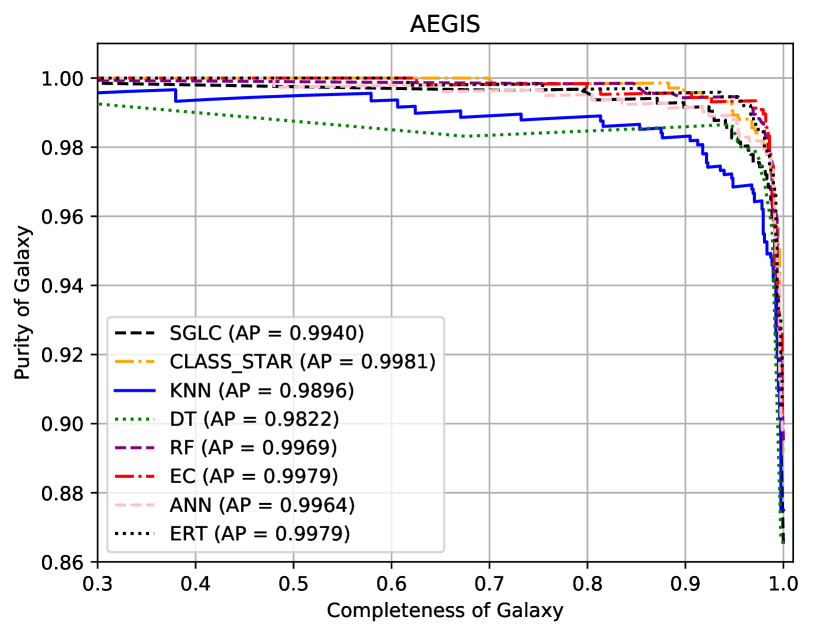
As said earlier, miniJPAS consists of 4 fields, each of approximately 0.25 deg² field-of-view (for details see Bonoli et al., 2020). The mJP-AEGIS1 has 20016 objects and features an $r$-band PSF which is similar to mJP-AEGIS3 ($\sim$0.7”) and better than mJP-AEGIS2 and mJP-AEGIS4 ($\sim$0.8”). It is then interesting to repeat for mJP-AEGIS1 the analysis relative to HSC-SSP (see Section 5.2). We do not consider the analysis relative to SDSS as the crossmatched catalog would be too small.

The crossmatch of mJP-AEGIS1 with HSC-SSP in the range $18.5\leq r\leq 23.5$ has 4486 objects, 3809 galaxies and 677 stars. We show the results in Figure 16, which should be compared with the analysis that considers the full miniJPAS catalog in Figure 9. It is clear that the results relative to the various classifiers improve as expected. In particular, when considering both morphological and photometric features, ERT goes from $AUC=0.979$ (Fig. 9) to $AUC=0.987$ (Fig. 16).

Figure 16: ROC curves (left panels) and purity curves for galaxies (right panels) for the classifiers considered in this paper for the AEGIS1 field crossmatched with the HSC-SSP catalog in the magnitude interval $18.5\leq r\leq 23.5$. The top panels are relative to the analysis that uses only photometric bands while the bottom panels to the analysis that uses photometric bands and morphological parameters. For comparison it is shown also the classification by CLASS_STAR and SGLC that always use morphological parameters. Note that the axes ranges are varied in order to better show the curves.

Appendix D ADQL query

The value added catalog with the ERT and RF classifications is publicly available at j-pas.org/datareleases via the ADQL table minijpas.StarGalClass. The column ert_prob_star gives the probability $1-f$ of being a star provided by the ERT classifier, using both morphological and photometric information. The column rf_prob_star gives the probability $1-f$ of being a star provided by the RF classifier, using only photometric information. Note that here, in order to follow the convention of the minijpas.StarGalClass table, we are using the probability $1-f$ of being a star and not, as in the rest of this work, the probability $f$ of being a galaxy.

In order to facilitate access to our results we now report a simple query example that allows one to access the classifications generated by ML along with the miniJPAS photometric bands with flag and mask quality cuts:

SELECT

t1.MAG_AUTO[minijpas::uJAVA] as uJAVA,
t1.MAG_AUTO[minijpas::J0378] as J0378,
t1.MAG_AUTO[minijpas::J0390] as J0390,
t1.MAG_AUTO[minijpas::J0400] as J0400,
t1.MAG_AUTO[minijpas::J0410] as J0410,
t2.ert_prob_star,
t2.rf_prob_star

FROM

minijpas.MagABDualObj t1

JOIN

minijpas.StarGalClass t2

ON

t1.tile_id = t2.tile_id AND
t1.number=t2.number

WHERE

t1.flags[minijpas::rSDSS]=0 AND
t1.mask_flags[minijpas::rSDSS]=0

Appendix E Analysis using only morphology

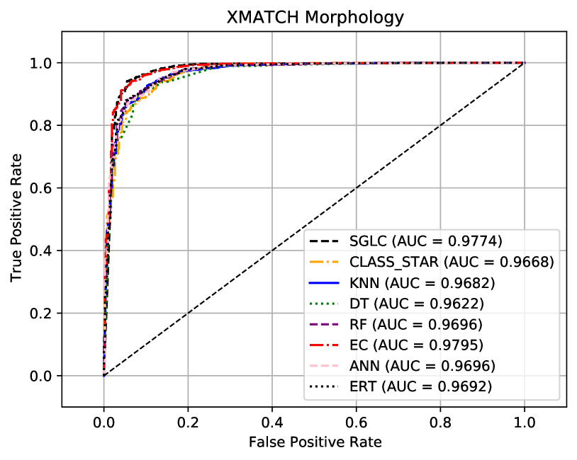
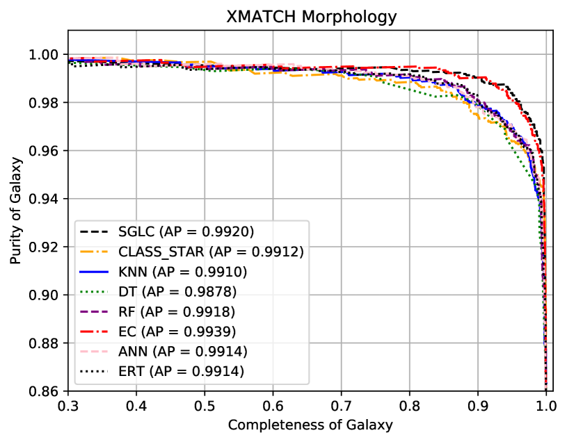
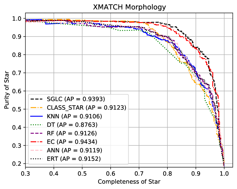
Here, we apply the ML methods discussed in the main text to the XMATCH catalog using only morphological parameters as input. In the Figure 17 one can see the performances of the different algorithms. Comparing these results with the ones of Figure 11 (morphology $+$ photometry), we observe that the inclusion of the photometric bands in the analysis increases the performance of the models. When using only morphological parameters the AUC, galaxy AP ad star AP of the best pure ML classifier are 0.9696, 0.9918 and 0.9152, respectively. Instead, when using morphological parameters and photometric bands the AUC, galaxy AP ad star AP of the best pure ML classifier are 0.9855, 0.9955 and 0.9615, respectively.

Figure 17: ROC curve (top panel) and purity curve for galaxies (middle panel) and stars (bottom panel) when using only morphological parameters in the magnitude range $15\leq r\leq 23.5$ of the XMATCH catalog.

Appendix F Hyperparameter optimization

The best values of the hyperparameters were found via the GridSearchCV method. They were selected according to the best mean from $k=10$ folds using the AUC-ROC metric. Below are the hyperparameters relative to the XMATCH catalog; the unspecified hyperparameters take the default values by scikit-learn version 0.23.1. We fixed random seed = 5.

F.1 Using photometric bands only

KNN

n_neighbors: 50, weights: distance

DT

class_weight: balanced, criterion: gini,
max_depth: 5, max_features: None, random_state: 5

RF

n_estimators: 100, bootstrap: True, class_weight:
balanced_subsample, criterion: entropy,
max_depth: 10, max_features: None

ANN

activation: logistic, hidden_layer_sizes: 200,
learning_rate: constant, solver: adam,
max_iter: 200, tol=0.0001

ERT

n_estimators: 200, bootstrap: False,
class_weight: balanced_subsample, criterion:
entropy, max_depth: 20, max_features: None

F.2 Using morphological parameters only

KNN

n_neighbors: 100, weights: distance

DT

class_weight: balanced, criterion: entropy,
max_depth: 5, max_features: None


RF

bootstrap: True, class_weight: balanced_
subsample, criterion: entropy, max_depth: 5,
max_features: None, ’n_estimators’: 100


ANN

activation: relu, hidden_layer_sizes: 200,
learning_rate: constant, solver: adam,
max_iter: 200, tol=0.0001

ERT

bootstrap: False, class_weight: balanced_
subsample, criterion: entropy, max_depth: 10,
max_features: None, n_estimators: 200

F.3 Using photometric bands together morphology parameters

KNN

n_neighbors: 100, weights: distance

DT

class_weight: balanced, criterion: entropy,
max_depth: 5, max_features: None

RF

n_estimators: 100, bootstrap: True,
class_weight: balanced_subsample,
criterion: entropy, max_depth: 20,
max_features: None

ANN

activation: logistic, hidden_layer_sizes:
200, learning_rate: constant, solver: sgd,
max_iter: 200, tol=0.0001

ERT

n_estimators: 200, bootstrap: False,
class_weight: balanced_subsample, criterion:
entropy, max_depth: 20, max_features: None

References

- Aihara et al. (2019) Aihara, H., AlSayyad, Y., Ando, M., et al. 2019, PASJ, 71, 114, [1905.12221].
- Alam et al. (2015) Alam, S., Albareti, F. D., Allende Prieto, C., et al. 2015, ApJS, 219, 12, [1501.00963].
- Altman (1992) Altman, N. 1992, American Statistician, 46, 175.
- Amorín et al. (2010) Amorín, R. O., Pérez-Montero, E., & Vílchez, J. M. 2010, ApJ, 715, L128, [1004.4910].
- Banerji et al. (2010) Banerji, M., Lahav, O., Lintott, C. J., et al. 2010, MNRAS, 406, 342, [0908.2033].
- Benitez et al. (2014) Benitez, N. et al. , [1403.5237].
- Bertin & Arnouts (1996) Bertin, E. & Arnouts, S. 1996, Astron. Astrophys. Suppl. Ser., 117, 393.
- Bilicki et al. (2018) Bilicki, M., Hoekstra, H., Brown, M. J. I., et al. 2018, A&A, 616, A69, [1709.04205].
- Biswas et al. (2013) Biswas, R., Blackburn, L., Cao, J., et al. 2013, Phys. Rev. D, 88, 062003, [1303.6984].
- Bonoli et al. (2020) Bonoli, S. et al. , [2007.01910].
- Breiman (2001) Breiman, L. 2001, Machine learning, 45, 5.
- Breiman et al. (1984) Breiman, L., Friedman, J. H., Olshen, R. A., & Stone, C. J. 1984, International Group, 432, 151.
- Cabayol et al. (2019) Cabayol, L., Sevilla-Noarbe, I., Fernández, E., et al. 2019, MNRAS, 483, 529, [1806.08545].
- Cardamone et al. (2009) Cardamone, C., Schawinski, K., Sarzi, M., et al. 2009, MNRAS, 399, 1191, [0907.4155].
- Carrillo et al. (2015) Carrillo, M., González, J. A., Gracia-Linares, M., & Guzmán, F. S. 2015, in Journal of Physics Conference Series, Vol. 654, Journal of Physics Conference Series, 012001
- Cavuoti et al. (2015) Cavuoti, S., Brescia, M., Tortora, C., et al. 2015, MNRAS, 452, 3100, [1507.00754].
- Cenarro et al. (2010) Cenarro, A. J., Moles, M., Cristóbal-Hornillos, D., et al. 2010, Society of Photo-Optical Instrumentation Engineers (SPIE) Conference Series, Vol. 7738, The Javalambre Astrophysical Observatory project, 77380V
- Charnock & Moss (2017) Charnock, T. & Moss, A. 2017, supernovae: Photometric classification of supernovae
- Costa-Duarte et al. (2019) Costa-Duarte, M. V., Sampedro, L., Molino, A., et al. 2019, , [1909.08626].
- Davis et al. (2007) Davis, M. et al. 2007, Astrophys. J., 660, L1, [astro-ph/0607355].
- Dawson et al. (2013) Dawson, K. S. et al. 2013, Astron. J., 145, 10, [1208.0022].
- Díaz-García et al. (2019) Díaz-García, L. A., Cenarro, A. J., López-Sanjuan, C., et al. 2019, A&A, 631, A156, [1711.10590].
- Fadely et al. (2012) Fadely, R., Hogg, D. W., & Willman, B. 2012, ApJ, 760, 15, [1206.4306].
- Garofalo et al. (2016) Garofalo, M., Botta, A., & Ventre, G. 2016, Proceedings of the International Astronomical Union, 12, 345–348.
- Gauci et al. (2010) Gauci, A., Adami, K. Z., Abela, J., & Magro, A. , [1005.0390].
- Geurts et al. (2006) Geurts, P., Ernst, D., & Wehenkel, L. 2006, Machine learning, 63, 3.
- Hastie et al. (2009) Hastie, T., Tibshirani, R., & Friedman, J. 2009, The elements of statistical learning: data mining, inference, and prediction (Springer Science & Business Media)
- Henrion et al. (2011) Henrion, M., Mortlock, D. J., Hand, D. J., & Gand y, A. 2011, MNRAS, 412, 2286, [1011.5770].
- Ishak (2017) Ishak, B. 2017, Contemporary Physics, 58, 99.
- Kim & Brunner (2017) Kim, E. J. & Brunner, R. J. 2017, MNRAS, 464, 4463, [1608.04369].
- Kim et al. (2015) Kim, E. J., Brunner, R. J., & Carrasco Kind, M. 2015, MNRAS, 453, 507, [1505.02200].
- Le Fevre et al. (1995) Le Fevre, O., Crampton, D., Lilly, S. J., Hammer, F., & Tresse, L. 1995, Astrophys. J., 455, 60, [astro-ph/9507011].
- Lochner et al. (2016) Lochner, M., McEwen, J. D., Peiris, H. V., Lahav, O., & Winter, M. K. 2016, ApJS, 225, 31, [1603.00882].
- López-Sanjuan et al. (2019) López-Sanjuan, C., Vázquez Ramió, H., Varela, J., et al. 2019, A&A, 622, A177, [1804.02673].
- Marshall et al. (2017) Marshall, P., Anguita, T., Bianco, F. B., et al. , [1708.04058].
- Matthews et al. (2013) Matthews, D. J., Newman, J. A., Coil, A. L., Cooper, M. C., & Gwyn, S. D. J. 2013, ApJS, 204, 21, [1210.2405].
- Mitchell (1997) Mitchell, T. M. 1997, Machine learning
- Moles et al. (2008) Moles, M., Benítez, N., Aguerri, J. A. L., et al. 2008, AJ, 136, 1325, [0806.3021].
- Molino et al. (2014) Molino, A. et al. 2014, Mon. Not. Roy. Astron. Soc., 441, 2891, [1306.4968].
- Newman et al. (2013) Newman, J. A., Cooper, M. C., Davis, M., et al. 2013, ApJS, 208, 5, [1203.3192].
- Odewahn et al. (2004) Odewahn, S. C., de Carvalho, R. R., Gal, R. R., et al. 2004, AJ, 128, 3092.
- Pedregosa et al. (2011) Pedregosa, F. et al. 2011, J. Machine Learning Res., 12, 2825, [1201.0490].
- Rumelhart et al. (1986) Rumelhart, D. E., Hinton, G. E., & Williams, R. J. 1986, Nature, 323, 533.
- Sevilla-Noarbe et al. (2018) Sevilla-Noarbe, I., Hoyle, B., Marchã, M. J., et al. 2018, MNRAS, 481, 5451, [1805.02427].
- Vargas dos Santos et al. (2020) Vargas dos Santos, M., Quartin, M., & Reis, R. R. 2020, Mon. Not. Roy. Astron. Soc., 497, 2974, [1908.04210].
- Vasconcellos et al. (2011) Vasconcellos, E. C., de Carvalho, R. R., Gal, R. R., et al. 2011, AJ, 141, 189, [1011.1951].
- Whitten et al. (2019) Whitten, D. D., Placco, V. M., Beers, T. C., et al. 2019, A&A, 622, A182, [1811.02279].
- Wolpert (1996) Wolpert, D. H. 1996, Neural Computation, 8, 1341.