Bayesian Optimization of Risk Measures 111To appear in NeurIPS 2020.
Abstract
We consider Bayesian optimization of objective functions of the form , where is a black-box expensive-to-evaluate function and denotes either the VaR or CVaR risk measure, computed with respect to the randomness induced by the environmental random variable . Such problems arise in decision making under uncertainty, such as in portfolio optimization and robust systems design. We propose a family of novel Bayesian optimization algorithms that exploit the structure of the objective function to substantially improve sampling efficiency. Instead of modeling the objective function directly as is typical in Bayesian optimization, these algorithms model as a Gaussian process, and use the implied posterior on the objective function to decide which points to evaluate. We demonstrate the effectiveness of our approach in a variety of numerical experiments.
1 Introduction
Traditional Bayesian optimization (BO) has focused on problems of the form , or more generally, , where is a time-consuming black box function that does not provide derivatives, and is a random variable. This has seen an enormous impact, and has expanded from hyper-parameter tuning [1, 2] to more sophisticated applications such as drug discovery and robot locomotion [3, 4, 5, 6]. However, in many truly high-stakes settings, optimizing average performance is inappropriate: we must be risk-averse. In such settings, risk measures have become a crucial tool for quantifying risk. For instance, by law, banks are regulated using the Value-at-Risk [7]. Risk measures have also been used in cancer treatment planning [8, 9], healthcare operations [10], natural resource management [11], disaster management [12], data-driven stochastic optimization [13], and risk quantification in stochastic simulation [14].
In this work, we consider risk averse optimization of the form , where is a risk measure that maps the probability distribution of (induced by the randomness on ) onto a real number describing its level of risk. We focus on the setting, where, during the evaluation stage, can be evaluated for any , e.g., using a simulation oracle. After the evaluation stage, we choose a decision to be implemented in the real world, nature chooses the random , and the objective is then realized.
When is inexpensive and has convenient analytic structure, optimizing against a risk measure is well understood [15, 16, 17, 18]. However, when is expensive-to-evaluate, derivative-free, or is a black box, the existing literature is inadequate in answering the problem. A naive approach would be to use the standard BO algorithms with observations of . However, a single evaluation of the objective function, , requires multiple evaluations of , which can be prohibitively expensive when the evaluations of are expensive. For example, if each evaluation of takes one hour, and we need samples to obtain a high-accuracy estimate of , a single evaluation of the objective function would require more than four days. Moreover, if we do not obtain a high-accuracy estimate, estimators are typically biased [19] in a way that is unaccounted for by traditional Gaussian process regression. For the risk measure Value-at-Risk, the recent work of [20] addresses this issue by modeling using individual observations of . However, their method only chooses the to evaluate, and is randomly set according to its environmental distribution. As evidenced by [21, 22], jointly selecting and to evaluate offers significant improvements to query efficiency. This ability, unlocked when evaluations are made using a simulation oracle, is leveraged by the methods we introduce here.
As an example of the benefits of choosing intelligently, consider a function that is monotone in . To optimize VaR of , we only need to evaluate a single value of , the one that corresponds to the VaR, and evaluating any other is simply inefficient. In a black-box setting, we would not typically know that was monotone but, by modeling directly, we can discover the regions of that matter and focus most of our effort into selectively evaluating from these regions.
In this paper, we focus on two risk measures commonly used in practice, Value-at-Risk (VaR) and Conditional Value-at-Risk (CVaR); and develop a novel approach that overcomes the aforementioned challenges. Our contributions are summarized as follows:
-
•
To the best of our knowledge, our work is the first to consider BO of risk measures while leveraging the ability to choose and at query time. The selection of enables efficient search of the solution space, and is a significant contributor to the success of our algorithms.
-
•
We provide a novel one-step Bayes optimal algorithm , and a fast approximation that performs well in numerical experiments; significantly improving the sampling efficiency over the state-of-the-art BO methods.
-
•
We combine ideas from different strands of literature to derive gradient estimators for efficient optimization of and , which are shown to be asymptotically unbiased and consistent.
-
•
To further improve the computational efficiency, we propose a two time scale optimization approach, that is broadly applicable for optimizing acquisition functions whose computation involves solving an inner optimization problem.
The remainder of this paper is organized as follows. Section 2 provides a brief background on BO and risk measures. Section 3 formally introduces the problem setting. Section 4 introduces the statistical model on , a Gaussian process (GP) prior, and explains how to estimate VaR and CVaR of a GP. Section 5 introduces , a knowledge gradient type of acquisition function for optimization of VaR and CVaR, along with a cheaper approximation, , and efficient optimization of both acquisition functions. Section 6 presents numerical experiments demonstrating the performance of the algorithms developed here. Finally, the paper is concluded in Section 7.
2 Background
2.1 Bayesian optimization
BO is a framework for global optimization of expensive-to-evaluate, black-box objective functions [23], whose origins date back to the seminal work of [24]. Among the various types of acquisition functions in BO [25, 26, 27], our proposed acquisition functions can be catalogued as knowledge gradient methods, which have been key to extending BO beyond the classical setting, allowing for parallel evaluations [28], multi-fidelity observations [29], and gradient observations [30].
Within the BO literature, a closely related work to ours is [22], which studies the optimization of , while jointly selecting and to evaluate. Due to linearity of the expectation, the GP prior on translates into a GP prior on , a fact that is leveraged to efficiently compute the one-step Bayes optimal policy, also known as the knowledge gradient (KG) policy. Although it is not the focus of this study, since CVaR at risk level is the expectation, our methods can be directly applied for solving the expectation problem, and the resulting algorithm is equivalent to the algorithm proposed in [22].
Our work also falls within a strand of the BO literature that aims to find solutions that are risk-averse to the effect of an unknown environmental variable [31, 32, 20, 33, 34]. Worst-case optimization, also known as minimax or robust optimization, is considered by [31] and [32], whereas [33] and [34] consider distributionally robust optimization [35]. Within this line of research, [20], which studies the optimization of , is arguably the most closely related to work. Like our statistical model, their model is also built using individual observations of and not directly using observations of . However, unlike our approach, their approach is only able to choose at which to evaluate. Our approach jointly chooses and to evaluate, which is critical when is large. Moreover, our model allows for noisy evaluations of , which could introduce additional bias in their model.
2.2 Risk measures
We recall that a risk measure (cf. [36, 37, 38, 39]) is a functional that maps probability distributions onto a real number. Risk measures offer a middle ground between the risk-neutral expectation operator and the worst-case performance measure, which is often more interpretable than expected utility [13]. For a generic random variable , we often use the notation to indicate the risk measure evaluated on the distribution of .
The most widely used risk measure is VaR [40], which measures the maximum possible loss after excluding worst outcomes with a total probability of , and is defined as where indicates the distribution of . Another widely used risk measure is CVaR, which is the expectation of the worst losses with a total probability of , and is given by .
VaR and CVaR have been applied in a wide range of settings, including simulation optimization under input uncertainty [13, 18], insurance [41] and risk management [42]. They are widely used in finance, and VaR is encoded in the Basel II accord [43]. We refer the reader to [44] for a broader discussion on VaR and CVaR.
3 Problem setup
We consider the optimization problem
| (1) |
where is a simple compact set, e.g., a hyper-rectangle; is a random variable with probability distribution and compact support ; and is a known risk measure, mapping the random variable (induced by ) to a real number. We assume that is a continuous black-box function whose evaluations are expensive, i.e., each evaluation takes hours or days, has significant monetary cost, or the number of evaluations is limited for some other reason. We also assume that evaluations of are either noise-free or observed with independent normally distributed noise with known variance.
We emphasize that the risk measure is only over the randomness in , and is calculated holding fixed. For example, if is VaR, and is a continuous random variable with density , then this is explicitly written as:
| (2) |
Later, we will model as being drawn from a GP, but we will continue to compute only over the randomness in . Thus, this quantity is a function of and , and will be random with a distribution induced by the distribution on (and more precisely by the distribution on ).
4 Statistical model
We assume a level of familiarity with GPs and refer the reader to [45] for details. We place a GP prior on , specified by a mean function and a positive definite covariance function , and assume that queries of are of the form , where is independent across evaluations. The posterior distribution on given the history after evaluations, , is again a GP with mean and covariance functions and , which can be computed in closed form in terms of and .
The GP posterior distribution on implies a posterior distribution on the mapping . In contrast with the case where is the expectation operator, this distribution is, in general, non-Gaussian, rendering computations more challenging. As we discuss next, however, quantities of interest can still be computed following a simple Monte Carlo (MC) approach. Specifically, we discuss how to compute the posterior mean of , i.e., , where denotes the conditional expectation given .
Our approach to estimating the value of builds on samples of drawn from the posterior, and the corresponding implied values of . For the purposes of this discussion, we assume is finite and small, say , and that is uniform over . When the cardinality of is finite but large or is continuous, we instead use a set of i.i.d. samples drawn from .
Denote and . The time- joint posterior distribution of is normal with mean vector and covariance matrix . A sample from this distribution can be obtained via the reparameterization trick [46], i.e., as , where is is the Cholesky factor of and is drawn from the -variate standard normal distribution.
Let denote a realization of , computed as described above. The corresponding MC estimate of can be calculated as the empirical risk measure corresponding to this realization, which, under the assumption that is uniform over , can obtained by ordering the coordinates of so that , and letting
| (3) |
be the empirical VaR and CVaR respectively (cf. [44]), where is the ceiling operator. This can be easily extended to non-uniform discrete by accounting for the probability mass of each .
Finally, if and , , are samples of and , obtained as described above. Then, MC estimates of and are given by and , respectively.
5 The acquisition function
As is standard in the BO literature, our algorithm’s search is guided by an acquisition function, whose maximization indicates the next point to evaluate. Our proposed acquisition function generalizes the well-known knowledge gradient acquisition function [26], which has been generalized to other settings such as parallel and multi-fidelity optimization [28, 29].
Before formally introducing our acquisition function, we note that, in our setting, choosing a decision to be implemented after the evaluation stage is complete, is not a straightforward task. If the cardinality of is large, then the chances are will not be known exactly as this would require evaluating for all . A common approach in such scenarios is to choose the decision with best expected objective value according to the posterior distribution (c.f. [23]),
| (4) |
Having defined the choice of the decision to be implemented after the evaluation stage is complete, we can now introduce our acquisition function, the knowledge gradient for risk measures. We motivate this acquisition function by noting that, if we had to choose a decision with the information available at time , the expected objective value we would get according to equation (4) is simply On the other hand, if we were allowed to make one additional evaluation, the expected objective value we would get is . Therefore, measures improvement due to making one additional evaluation.
We emphasize that, given the information available at time , is random due to its dependence on the yet unobserved -st evaluation. The knowledge gradient for risk measures acquisition function is defined as the expected value of given the information available at time and the next point to evaluate, termed the "candidate" from here on:
| (5) |
Our algorithm sequentially chooses the next point to evaluate as the candidate that maximizes (5), and is, by construction, one-step Bayes optimal.
5.1 Optimization of
In this section, we discuss how to evaluate and optimize using a sample average approximation (SAA) approach [47]. In a nutshell, this approach works by constructing a MC approximation of , that is deterministic given a finite set of base samples not depending on the candidate . Such an approximation can be optimized using deterministic optimization methods. This is usually faster than optimizing the original acquisition function with stochastic optimization techniques. Below, we discuss how to construct this SAA. Moreover, we show that its gradients can be readily computed, thus allowing the use of higher-order optimization methods. A more detailed discussion of our approach to optimize can be found in the supplement.
We begin by noting that does not depend on the candidate being evaluated. Therefore, maximizing is equivalent to solving
| (6) |
The first step in building an SAA of (6) is to draw fantasy samples from the time- posterior distribution on , which, conditioned on , is Gaussian with mean and variance . Using the reparameterization trick, these samples can be obtained as , , where the base samples are drawn from a standard normal distribution. These samples give rise to fantasy GP models of the posterior distribution at time , obtained by conditioning the GP model on the event and , i.e., by adding as the hypothetical -st observation.
For each fantasy GP model , an MC estimate of , , can be constructed by averaging samples as described in Section 4. Let denote the -th such sample corresponding to the -th fantasy GP model, where the dependence of on the candidate and is made implicit. Additional base samples needed to define are generated once and held fixed so that it becomes a deterministic function of . The SAA of (6) is then given by
| (7) |
In the supplement, we show that the gradient of with respect to , denoted , can be computed explicitly as and for VaR and CVaR respectively, where this notation is defined explicitly in the supplement. We use these gradients within the LBFGS algorithm [48] to solve the inner optimization problems in (7). Moreover, we show that, under mild regularity conditions, the envelope theorem ([49], Corollary 4) can be used to express the gradient of the objective in (7) as
| (8) |
where denotes the gradient of with respect to evaluated at , and is a solution to the -th inner optimization problem in (7). Again, we use these gradients within LBFGS to solve (7). In addition, we also show that the above gradients are asymptotically unbiased and consistent gradient estimators as . Therefore, can be maximized using (multi-start) stochastic gradient ascent (SGA), following an approach similar to a proposal in [30].
Proposition 1.
Under suitable regularity conditions, (8) is an asymptotically unbiased and consistent estimator of the gradient of as .
A formal statement of the proposition and its proof is given in the supplement for the case of . It is also shown that selecting the -th candidate to evaluate using the algorithm, including the training of the GP model, has a computational complexity of , where are the number of LBFGS [48] iterations performed for training the GP model, and the outer and inner optimization loops respectively.
Remark 1.
5.2 The approximation
The algorithm is computationally intensive, as it requires solving a nested non-convex optimization problem. In a wide range of settings, the sampling efficiency it provides justifies its computational cost, but in certain not-so-expensive settings, a faster algorithm is desirable.
Inspired by the EI [25] and KGCP [26] acquisition functions, we propose , which replaces the inner optimization problem of with a much simpler one. In , the inner optimization is restricted to the points that have been evaluated for at least one , denoted by , and the resulting value of the optimization problem is . The intuition behind this is that the GP model is an extrapolation of the data. Thus, these points carry an immense amount of information on the GP model and the posterior objective, which makes them an ideal set of candidates to consider. The resulting approximation to is,
| (9) |
We note that, like , has an appealing one-step Bayes optimal interpretation; the maximizer of is the one-step optimal point to evaluate if we restrict the choice of the decision to be implemented, , among those that have been evaluated for at least one environmental condition, .
5.3 Two time scale optimization
In this paper, we introduce two acquisition functions, and . These acquisition functions share a nested structure, making their maximization computationally challenging. Here, we describe a novel two time scale optimization approach for reducing this computational burden.
Since the posterior mean and kernel are continuous functions of the data, if we fix the base samples used to generate the fantasy model and the GP sample path, a small perturbation to the candidate solution results in only a slight shift to the sample path. Thus, the optimal solutions to the inner problems, obtained using the previous candidate solution, should remain within a small neighborhood of a current high quality local optimal solution (and likely of the global solution). We can thus use the inner solutions obtained in the previous iteration to obtain a good approximation of the acquisition function value and its gradient for the current candidate. We utilize this observation by solving the inner optimization problem once every iterations, and using this solution to evaluate for the remaining iterations. We refer to this approach as two time scale optimization and present an algorithmic description with more detail in the supplement.
The two time scale optimization approach outlined here is not limited to , and can be applied to other acquisition functions that require nested optimization, such as [26, 51, 22]. In numerical testing, the two-time-scale optimization approach did not affect the performance of either of our algorithms while offering significant computational savings.
5.4 A visual analysis of the acquisition functions
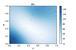
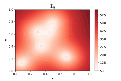
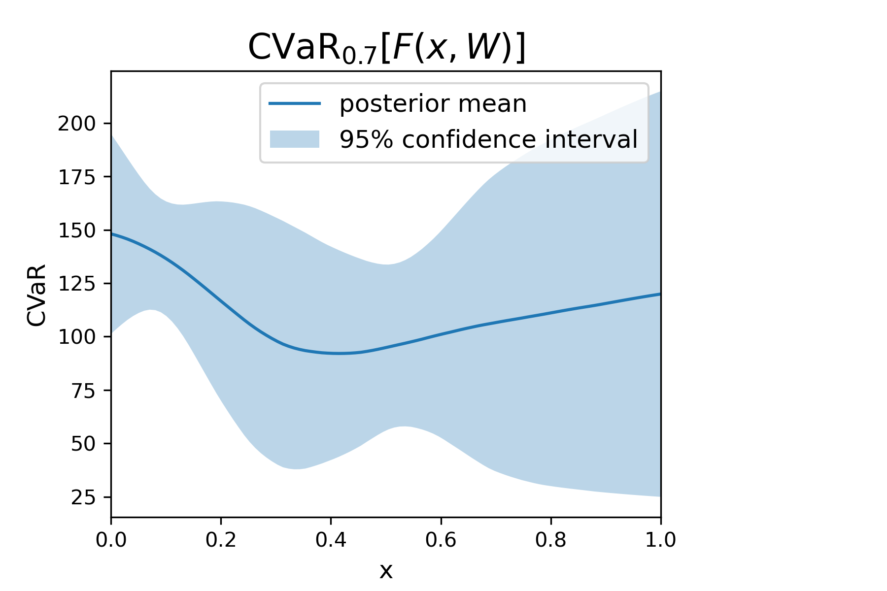
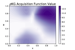
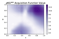
Figure 1 plots a GP model based on 6 random samples taken from a 2-dim test function and the corresponding acquisition function values of and over . We use a CVaR objective with risk level and a uniform distribution over .
First, observe that the plot closely resembles , supporting our claim that it is a good approximation. Second, the implied posterior on the objective shows a large uncertainty for larger values of , and we expect a large for these to encourage exploration. plots show that this is indeed the case, while also showing a large variation along the axis. In this region of , the posterior uncertainty is much larger for larger values of . These also happen to have a posterior mean near likely -quantiles of , making them more informative about CVaR. Indeed, prefers these , reaching a maximum near .
Another area of interest is the promising region of , as it contains the minimizer of the current posterior mean of the objective. We observe both a posterior mean substantially below the likely -quantiles of and a low posterior uncertainty for in this region, making them less useful for estimating CVaR, and correspondingly low . However, the at the two ends of the range are more likely to be near an -quantile and have larger uncertainty. Thus, an observation from these would help pinpoint the exact location of the minimizer of the posterior expectation of the objective and thus are associated with larger .
We hope that these plots and accompanying discussion help the reader appreciate the value of considering the environmental variable, , in designing the acquisition function.
6 Numerical experiments
In this section, we present several numerical examples that demonstrate the sampling efficiency of our algorithms. We compare our algorithms with the Expected Improvement (EI, [25]), Knowledge Gradient (KG, [51]), Upper Confidence Bound (UCB), and Max Value Entropy Search (MES, [52]) algorithms. We use the readily available implementations from the BoTorch package [53], and the default parameter values given there. The benchmark algorithms cannot utilize observations of while optimizing . Therefore, for these algorithms, we fit a GP on observations of , which are obtained by evaluating a given for all (or a subset ) and then calculating the value of the risk measure on these samples. As a result, the benchmark algorithms require (or ) samples per iteration whereas and require only one. We could not compare with [20] since the code was not available at the time of the writing of this paper.
We optimize each acquisition function using the LBFGS [48] algorithm with restart points. The restart points are selected from raw samples using a heuristic. For the inner optimization problem of , we use random restarts with raw samples. For both and , we use the two time scale optimization where we solve the inner optimization problem once every optimization iterations. and are both estimated using fantasy GP models, and sample paths for each fantasy model.
We initialize each run of the benchmark algorithms with starting points from the space, and the corresponding evaluations of obtained by evaluating for each (or , to be specified for each problem). The GP models for and are initialized using the equivalent number of evaluations, with randomly drawn from . Further details on experiment settings is given in the supplement. The code for our implementation of the algorithms and experiments can be found at https://github.com/saitcakmak/BoRisk.
6.1 Synthetic test problems
The first two problems we consider are synthetic test functions from the BO literature. The first problem is the 4-dim Branin-Williams problem in [54]. We consider minimization of both VaR and CVaR at risk level with respect to the distribution of environmental variables . The second problem we consider is the 7-dim function from [31]. We formulate this problem for minimization of CVaR at risk level with respect to the distribution of the -dim environmental variable . More details on these two problems can be found in the supplement.
6.2 Portfolio optimization problem
In this test problem, our goal is to tune the hyper-parameters of a trading strategy so as to maximize return under risk-aversion to random environmental conditions. We use CVXPortfolio [55] to simulate and optimize the evolution of a portfolio over a period of four years using open-source market data. Each evaluation of this simulator returns the average daily return over this period of time under the given combination of hyper-parameters and environmental conditions. The details of this simulator can be found in Sections 7.1-7.3 of [55].
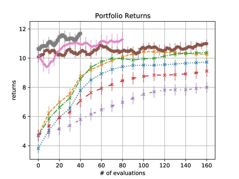
The hyper-parameters to be optimized are the risk and trade aversion parameters, and the holding cost multiplier over the ranges , , and , respectively. The environmental variables are the bid-ask spread and the borrow cost, which we assume are uniform over and , respectively. For this problem, we use the VaR risk measure at risk level We use a random subset of size for the inner computations of our algorithms, and a random subset of size is used for the evaluations of by the benchmark algorithms.
Since this simulator is indeed expensive-to-evaluate, with each evaluation taking around 3 minutes, evaluating the performance of the various algorithms becomes prohibitively expensive. Therefore, in our experiments we do not use the simulator directly. Instead, we build a surrogate function obtained as the mean function of a GP trained using evaluations of the actual simulator across points chosen according to a Sobol sampling design [50].
|
|
|
|
|
|
6.3 Allocating COVID-19 testing capacity
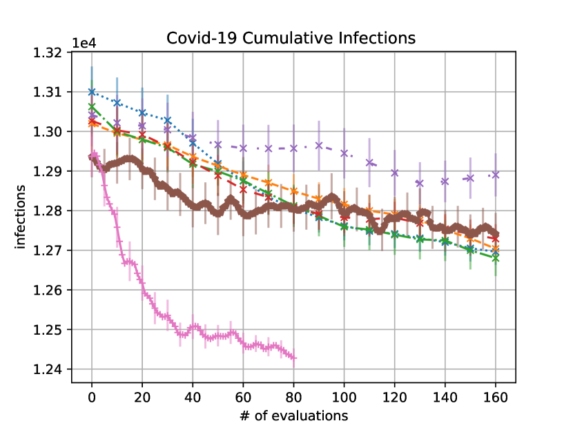
In this example, we study allocation of a joint COVID-19 testing capacity between three neighboring populations (e.g., cities, counties). The objective is to allocate the testing capacity between the populations to minimize the total number of people infected with COVID-19 in a span of two weeks. We use the COVID-19 simulator provided in [56] and discussed in [57, 58]. The simulator models the interactions between individuals within the population, the disease spread and progression, testing and quarantining of positive cases. Contact tracing is performed for people who test positive, and the contacts that are identified are placed in quarantine.
We study three populations of sizes , , and that share a combined testing capacity of tests per day. The initial disease prevalence within each population is estimated to be in the range of and respectively. We assign a probability of to the middle of the range and to the two extremes, independently for each population. Thus, the initial prevalence within each population defines the environmental variables. We pick the fraction of testing capacity allocated to the first two populations as the decision variable (remaining capacity is allocated to the third), with the corresponding decision space . For the inner computations of , we use the full set, however, for the evaluations of benchmark algorithms we randomly sample a subset of size to avoid using evaluations per iteration.
6.4 Results
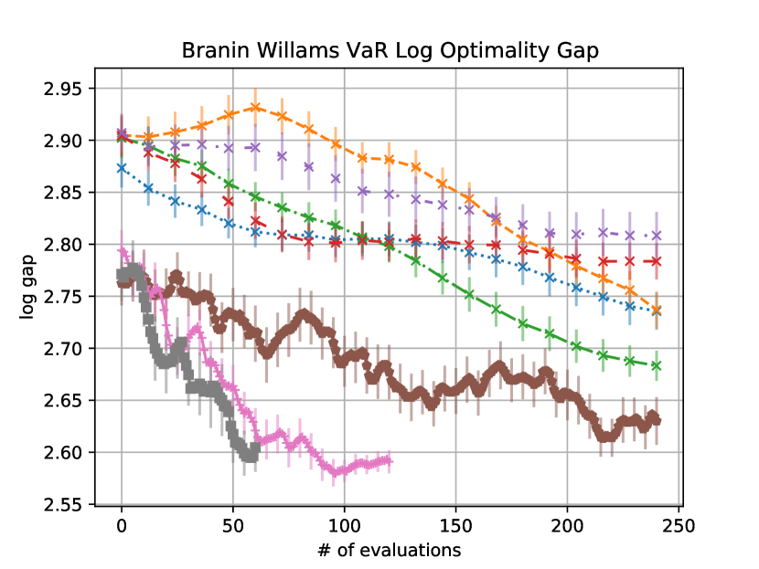
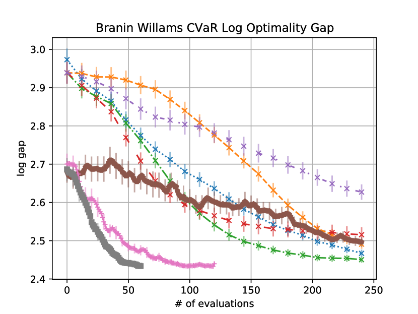
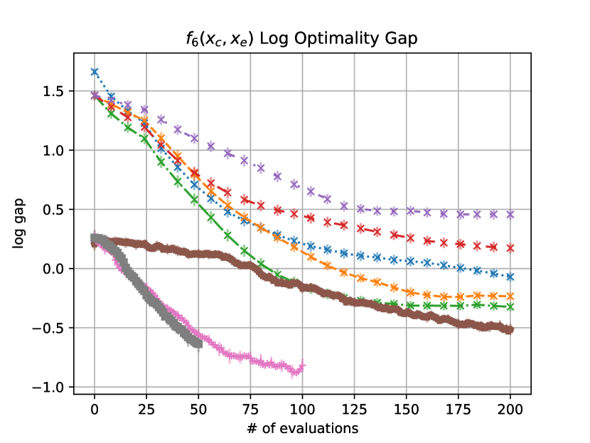
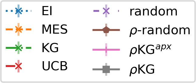
Figure 2 plots results of the experiments. Evaluations reported exclude the GP initialization, and the error bars denote one standard error. In each experiment, and match or beat the performance of all benchmarks using less than half as many function evaluations, thus, demonstrating superior sampling efficiency. In the experiments was intentionally kept small (between 8-12) to avoid giving our methods an outsized advantage. If were larger, the benchmarks would use up even more evaluations per iteration, and our algorithms would provide an even larger benefit.
To demonstrate the benefit of using our novel statistical model, we included experiments with two random sampling strategies. The one labeled “random” evaluates , and uses the corresponding GP model over . “-random”, on the other hand, evaluates at a randomly selected , uses our statistical model, and reports as the solution. The ability to survey the whole space gives “-random" a significant boost. We see that, despite choosing evaluations randomly, it is highly competitive against all the benchmarks, and outperforms “random" by a significant margin. This demonstrates the added value of our statistical model, which captures all the information available in the data, and suggests an additional cheap-to-implement algorithm that is useful whenever is cheap enough to render other algorithms too expensive.
The supplement presents additional plots comparing algorithm run-times. Data from Branin Williams and show that even with only moderately expensive function evaluations (a few minutes per evaluation), our algorithms save time compared with the benchmarks presented here.
7 Conclusion
In this work, we introduced a novel Bayesian optimization approach for solving problems of the form , where is a risk measure and is a black-box function that can be evaluated for any . By modeling with a GP model instead of the objective function directly as is typical in Bayesian optimization, our approach is able to leverage more fine-grained information and, importantly, to jointly select both and at which to evaluate . This allows our algorithms to significantly improve sampling efficiency over existing Bayesian optimization methods.
We propose two acquisition functions, , which is one step-Bayes optimal, and a principled cheap approximation, , along with an efficient, gradient-based approach to optimize them. To further improve numerical efficiency, we introduced a two time scale optimization approach that is broadly applicable for acquisition functions that require a nested optimization.
Broader Impact
Our work is of interest whenever one needs to make a decision guided by an expensive simulator, and subject to environmental uncertainties. Such scenarios arise in simulation assisted medical decision making [4], in financial risk management [7, 59, 60], in public policy, and disaster management [61].
The impact of our algorithms could be summarized as facilitating risk averse decision making. In many scenarios, risk averse approaches result in decisions that are more robust to environmental uncertainties compared to decisions resulting from common risk neutral alternatives. For example, in a financial crisis, an earlier risk-averse decision of holding more cash and other low-risk securities might prevent large losses or even the default of a financial institution. As another example, a risk averse decision of stockpiling of excess medical supplies in non-crisis times would alleviate the shortages faces during crisis times, such as the COVID-19 pandemic we are facing today.
On the negative side of things, the risk averse decisions we facilitate may not always benefit all stakeholders. For a commercial bank, a risk averse approach may suggest a higher credit score threshold for making loans, which might end up preventing certain groups from access to much needed credit.
In our case, the failure of the system would mean a poor optimization of the objective, and recommendation of a bad solution. Implementation of a bad decision can have harmful consequences in many settings; however, we imagine that any solution recommended by our algorithms would then be evaluated using the simulator, thus preventing the implementation of said decision.
Our methods do not rely on training data, and only require noisy evaluations of the function value. Thus, it can be said that our method does not leverage any bias in any training data. However, the solutions recommended by our algorithms are only good up to the supplied function evaluations, thus are directly affected by any biases built into the simulator used for these evaluations.
Acknowledgements
The authors gratefully acknowledge the support by the National Science Foundation under Grants CAREER CMMI-1453934 and CCF-1740822; and the Air Force Office of Scientific Research under Grants FA9550-19-1-0283 and FA9550-15-1-0038. We also thank the anonymous reviewers, whose comments helped improve and clarify the presentation of our paper.
References
- [1] J. Snoek, H. Larochelle, and R. Adams, “Practical Bayesian optimization of machine learning algorithms,” Advances in Neural Information Processing Systems, pp. 2951–2959, December 2012.
- [2] M.-A. Zöller and M. F. Huber, “Benchmark and survey of automated machine learning frameworks,” arXiv 1904.12054, 2019.
- [3] D. Negoescu, P. Frazier, and W. Powell, “The knowledge-gradient algorithm for sequencing experiments in drug discovery,” INFORMS Journal on Computing, vol. 23, pp. 346–363, June 2011.
- [4] J. Xie, P. Frazier, S. Sankaran, A. Marsden, and S. Elmohamed, “Optimization of computationally expensive simulations with Gaussian processes and parameter uncertainty: Application to cardiovascular surgery,” 50th Annual Allerton Conference on Communication, Control, and Computing, October 2012.
- [5] B. Letham, B. Karrer, G. Ottoni, and E. Bakshy, Efficient tuning of online systems using Bayesian optimization, 2018. Available at https://research.fb.com/blog/2018/09/efficient-tuning-of-online-systems-using-bayesian-optimization/.
- [6] A. Rai, R. Antonova, F. Meier, and C. G. Atkeson, “Using simulation to improve sample-efficiency of Bayesian optimization for bipedal robots,” Journal of Machine Learning Research, vol. 20, no. 49, 2019.
- [7] J. A. Lopez, Regulatory Evaluation of Value-at-Risk Models, December 1997. Staff Report, Federal Reserve Bank of New York.
- [8] Y. An, J. Liang, S. E. Schild, M. Bues, and W. Liu, “Robust treatment planning with conditional value at risk chance constraints in intensity-modulated proton therapy,” Medical Physics, vol. 44, no. 1, 2017.
- [9] G. J. Lim, L. Kardar, S. Ebrahimi, and W. Cao, “A risk-based modeling approach for radiation therapy treatment planning under tumor shrinkage uncertainty,” European Journal of Operational Research, vol. 280, no. 1, pp. 266–278, 2020.
- [10] P. C. Austin and M. J. Schull, “Quantile regression: A statistical tool for out-of-hospital research,” Academic Emergency Medicine, vol. 10, no. 7, pp. 789–797, 2003.
- [11] S. A. Sethi and M. Dalton, “Risk measures for natural resource management: Description, simulation testing, and R code with fisheries examples,” Journal of Fish and Wildlife Management, 2012.
- [12] M. Meraklı and S. Küçükyavuz, “Risk aversion to parameter uncertainty in Markov decision processes with an application to slow-onset disaster relief,” IISE Transactions, vol. 52, no. 8, pp. 811–831, 2020.
- [13] D. Wu, H. Zhu, and E. Zhou, “A Bayesian risk approach to data-driven stochastic optimization: Formulations and asymptotics,” SIAM Journal on Optimization, vol. 28, no. 2, pp. 1588–1612, 2018.
- [14] H. Zhu, T. Liu, and E. Zhou, “Risk quantification in stochastic simulation under input uncertainty,” ACM Transactions on Modeling and Computer Simulation, vol. 30, no. 1, 2020.
- [15] A. Ruszczyński and A. Shapiro, “Optimization of risk measures,” in Probabilistic and Randomized Methods for Design under Uncertainty, pp. 119–157, Springer London, 2006.
- [16] A. Ben-Tal, L. El Ghaoui, and A. Nemirovski, Robust Optimization. Princeton University Press, 2009.
- [17] D. Bertsimas, D. Brown, and C. Caramanis, “Theory and applications of robust optimization,” SIAM Review, vol. 53, no. 3, pp. 464–501, 2011.
- [18] S. Cakmak, D. Wu, and E. Zhou, “Solving Bayesian risk optimization via nested stochastic gradient estimation,” arXiv: 2007.05860, 2020.
- [19] A. A. Trindade, S. Uryasev, A. Shapiro, and G. Zrazhevsky, “Financial prediction with constrained tail risk,” Journal of Banking & Finance, vol. 31, no. 11, pp. 3524 – 3538, 2007.
- [20] L. Torossian, V. Picheny, and N. Durrande, “Bayesian quantile and expectile optimisation,” arXiv: 2001.04833, 2020.
- [21] J. Janusevskis and R. Le Riche, “Simultaneous kriging-based estimation and optimization of mean response,” Journal of Global Optimization, 2013.
- [22] S. Toscano-Palmerin and P. I. Frazier, “Bayesian optimization with expensive integrands,” arXiv: 1803.08661, 2018.
- [23] P. I. Frazier, “A tutorial on Bayesian optimization,” in Recent Advances in Optimization and Modeling of Contemporary Problems, ch. 11, pp. 255–278, 2018.
- [24] H. J. Kushner, “A new method of locating the maximum point of an arbitrary multipeak curve in the presence of noise,” Journal of Basic Engineering, vol. 86, no. 1, pp. 97–106, 1964.
- [25] D. R. Jones, M. Schonlau, and W. J. Welch, “Efficient global optimization of expensive black-box functions,” Journal of Global Optimization, vol. 13, p. 455–492, December 1998.
- [26] W. Scott, P. Frazier, and W. Powell, “The correlated knowledge gradient for simulation optimization of continuous parameters using Gaussian process regression,” SIAM Journal on Optimization, vol. 21, no. 3, pp. 996–1026, 2011.
- [27] J. M. Hernández-Lobato, M. W. Hoffman, and Z. Ghahramani, “Predictive entropy search for efficient global optimization of black-box functions,” in Advances in Neural Information Processing Systems, pp. 918–926, 2014.
- [28] J. Wu and P. I. Frazier, “The parallel knowledge gradient method for batch Bayesian optimization,” in Advances Neural Information Processing Systems, p. 3134–3142, 2016.
- [29] M. Poloczek, J. Wang, and P. Frazier, “Multi-information source optimization,” in Advances in Neural Information Processing Systems, pp. 4288–4298, 2017.
- [30] J. Wu, M. Poloczek, A. G. Wilson, and P. I. Frazier, “Bayesian optimization with gradients,” in Proceedings of the 31st International Conference on Neural Information Processing Systems, p. 5273–5284, 2017.
- [31] J. Marzat, E. Walter, and H. Piet-Lahanier, “Worst-case global optimization of black-box functions through kriging and relaxation,” Journal of Global Optimization, vol. 55, pp. 707–727, 04 2013.
- [32] I. Bogunovic, J. Scarlett, S. Jegelka, and V. Cevher, “Adversarially robust optimization with Gaussian processes,” in Advances in Neural Information Processing Systems, pp. 5760–5770, 2018.
- [33] J. Kirschner, I. Bogunovic, S. Jegelka, and A. Krause, “Distributionally robust Bayesian optimization,” in Proceedings of the 23rd International Conference on Artificial Intelligence and Statistics, 2020.
- [34] T. T. Nguyen, S. Gupta, H. Ha, S. Rana, and S. Venkatesh, “Distributionally robust Bayesian quadrature optimization,” in Proceedings of the 23rd International Conference on Artificial Intelligence and Statistics, 2020.
- [35] H. Rahimian and S. Mehrotra, “Distributionally robust optimization: A review,” arXiv: 1908.05659, 2019.
- [36] P. Artzner, F. Delbaen, J.-M. Eber, and D. Heath, “Coherent measures of risk,” Mathematical Finance, vol. 9, no. 3, pp. 203–228, 1999.
- [37] R. Rockafellar and S. Uryasev, “Conditional value-at-risk for general loss distributions,” Journal of Banking & Finance, vol. 26, no. 7, pp. 1443 – 1471, 2002.
- [38] F. Delbaen, “Coherent risk measures on general probability spaces,” in Advances in Finance and Stochastics: Essays in Honour of Dieter Sondermann, pp. 1–37, Springer Berlin Heidelberg, 2002.
- [39] R. Rockafellar and S. Uryasev, “The fundamental risk quadrangle in risk management, optimization and statistical estimation,” Surveys in Operations Research and Management Science, vol. 18, p. 33–53, October 2013.
- [40] P. Jorion, Value at Risk: The New Benchmark for Managing Financial Risk. McGraw-Hill, 2007.
- [41] S. Zymler, B. Rustem, and D. Kuhn, “Robust portfolio optimization with derivative insurance guarantees,” European Journal of Operational Research, vol. 210, pp. 410–424, April 2011.
- [42] P. Jorion, Financial Risk Manager Handbook. Wiley, New York, 2010.
- [43] Basel Committee on Banking Supervision, “Fundamental review of the trading book,” Consultative Document, 2012.
- [44] L. J. Hong, Z. Hu, and G. Liu, “Monte carlo methods for value-at-risk and conditional value-at-risk: a review,” ACM Transactions on Modeling and Computer Simulation, vol. 24, no. 4, pp. 1–37, 2014.
- [45] C. E. Rasmussen and C. K. I. Williams, Gaussian Processes for Machine Learning. The MIT Press, 2006.
- [46] J. Wilson, F. Hutter, and M. Deisenroth, “Maximizing acquisition functions for Bayesian optimization,” in Advances in Neural Information Processing Systems, pp. 9884–9895, 2018.
- [47] S. Kim, R. Pasupathy, and S. G. Henderson, “A guide to sample average approximation,” in Handbook of Simulation Optimization, pp. 207–243, Springer New York, 2015.
- [48] C. Zhu, R. H. Byrd, P. Lu, and J. Nocedal, “Algorithm 778: L-bfgs-b: Fortran subroutines for large-scale bound-constrained optimization,” ACM Trans. Math. Softw., vol. 23, p. 550–560, December 1997.
- [49] P. Milgrom and I. Segal, “Envelope theorems for arbitrary choice sets,” Econometrica, vol. 70, no. 2, pp. 583–601, 2002.
- [50] A. B. Owen, “Scrambling Sobol’ and Niederreiter–Xing points,” Journal of Complexity, vol. 14, no. 4, pp. 466 – 489, 1998.
- [51] J. Wu and P. I. Frazier, “The parallel knowledge gradient method for batch Bayesian optimization,” in Advances in Neural Information Processing Systems, pp. 3134–3142, 2016.
- [52] Z. Wang and S. Jegelka, “Max-value entropy search for efficient Bayesian optimization,” in Proceedings of the 34th International Conference on Machine Learning, pp. 3627–3635, PMLR, 2017.
- [53] M. Balandat, B. Karrer, D. R. Jiang, S. Daulton, B. Letham, A. G. Wilson, and E. Bakshy, “BoTorch: Programmable Bayesian Optimization in PyTorch,” arXiv: 1910.06403, 2019.
- [54] B. Williams, T. Santner, and W. Notz, “Sequential design of computer experiments to minimize integrated response functions,” Statistica Sinica, vol. 10, pp. 1133–1152, October 2000.
- [55] S. Boyd, “Multi-period trading via convex optimization,” Foundations and Trends® in Optimization, vol. 3, no. 1, pp. 1–76, 2017.
- [56] M. Cashore, P. Frazier, Y. Zhang, and J. Wan, Group Testing, 2020. Available at https://github.com/peter-i-frazier/group-testing/.
- [57] P. Frazier, Y. Zhang, and M. Cashore, Feasibility of COVID-19 screening for the U.S. population with group testing, 2020. Available at https://docs.google.com/document/d/1hw5K5V7XOug_r6CQ0UYt25szQxXFPmZmFhK15ZpH5U0/.
- [58] L. Kotlikoff, Drs. Fauci & Birx: Here’s a way to contain Covid-19 and reopen the economy in as little as one month, May 2020. Available at https://www.forbes.com/sites/kotlikoff/2020/05/03/dr-fauci-heres-a-way-to-contain-covid-19-and-reopen-the-economy-in-as-little-as-one-month/.
- [59] A. J. McNeil, R. Frey, and P. Embrechts, Quantitative Risk Management: Concepts, Techniques and Tools. Princeton University Press, 2005.
- [60] M. B. Gordy and S. Juneja, “Nested simulation in portfolio risk measurement,” Management Science, vol. 56, no. 10, pp. 1833–1848, 2010.
- [61] D. Steward and T. T. H. Wan, “The role of simulation and modeling in disaster management,” Journal of Medical Systems, 2007.