From Spectrum Wavelet to Vertex Propagation: Graph Convolutional Networks Based on Taylor Approximation
Abstract
Graph convolutional networks (GCN) have been recently utilized to extract the underlying structures of datasets with some labeled data and high-dimensional features. Existing GCNs mostly rely on a first-order Chebyshev approximation of graph wavelet-kernels. Such a generic propagation model does not always suit the various datasets and their features. This work revisits the fundamentals of graph wavelet and explores the utility of signal propagation in the vertex domain to approximate the spectral wavelet-kernels. We first derive the conditions for representing the graph wavelet-kernels via vertex propagation. We next propose alternative propagation models for GCN layers based on Taylor expansions. We further analyze the choices of detailed graph representations for TGCNs. Experiments on citation networks, multimedia datasets and synthetic graphs demonstrate the advantage of Taylor-based GCN (TGCN) in the node classification problems over the traditional GCN methods.
Index Terms:
graph convolutional network, graph spectral wavelet, Taylor approximationI Introduction
Learning and signal processing over graph models have gained significant traction owing to their demonstrated abilities to capture underlying data interactions. Modeling each data point as a node and their interactions as edges in a graph, graph-based methods have been adopted in various signal processing and analysis tasks, such as semi-supervised classification [1, 2], spectral clustering [3, 4], link prediction [5] and graph classification [6]. For example, in [7], an undirected graph is constructed based on a Gaussian-distance model to capture geometric correlations among points in a point cloud, with which several graph-based filters have been developed to extract contour features of objects.
Among various graph-based tools, graph signal processing (GSP) has emerged as an efficient analytical tool for processing graph-modeled signals [8],[9]. Based on a graph Fourier space defined by the eigenspace of the representing adjacency or Laplacian matrix, GSP filters have found applications in practice, including bridge health monitoring [10], point cloud denoising [11], and image classification [12]. Leveraging graph Fourier transform [13], graph wavelet [14] and graph spectral convolution [15] can extract additional features from graph signals. For example, graph convolutional filters have been successful in edge detection and video segmentation [16].
Although GSP-based spectral filtering has demonstrated successes in a variety of applications, it still suffers from the high-complexity of spectrum computation and the need to select suitable propagation models. To efficiently extract signal features and integrate traditional GSP within the machine learning framework, graph convolutional networks (GCN) [1] have been developed for semi-supervised classification problems. Approximating graph spectral convolution with first-order Chebyshev expansions, GCN has been effective in such learning tasks. Furthermore, different GCN-related graph learning architectures, including personalized propagation of neural predictions (PPNP)[17] and N-GCN[18], have also been developed to process graph-represented datasets. However, some limitations remain with the traditional GCN based on Chebyshev expansions. For example, traditional GCN requires strong assumptions on maximum eigenvalues and Chebyshev coefficients for approximating spectral convolution, at the cost of possible information loss when compared against basic convolutional filters. Furthermore, systematic selection and design of graph representations for GCN remain elusive.
Our goal is to improve GCN by exploring its relationship with GSP. Specifically in this work, we explore the process from spectrum wavelet to vertex propagation, and investigate alternative designs for graph convolutional networks. Our contributions can be summarized as follows:
-
•
We revisit graph spectral convolution in GSP and define conditions for approximating spectrum wavelet via propagation in the vertex domain. These conditions could provide insights to design GCN layers.
-
•
We propose alternative propagation models for the GCN layers and develop a Taylor-based graph convolutional networks (TGCN) based on the aforementioned approximation conditions.
-
•
We illustrate the effectiveness of the proposed frameworks over several well-known datasets in comparison with other GCN-type and graph-based methods in node signal classification.
-
•
We also provide an interpretability discussion on the use of Taylor expansion, together with guidelines on selecting suitable graph representations for GCN layers.
In terms of the manuscript organization, we first provide an overview on graph-based tools and review the fundamentals of GCN in Section II and Section III, respectively. Next, we present the theoretical motivation and basic design of the Taylor-based graph convolutional networks (TGCN) in Section IV. Section V discusses the interpretability of Taylor expansion in approximation, and highlights the difference between TGCN and traditional GCN-based methods. We report the experimental results of the proposed TGCN framework on different datasets in Section VI, before concluding in Section VII.
II Related Work
In this section, we provide an overview on state-of-the-art graph signal processing (GSP) and graph convolutional networks (GCN).
II-A Graph Signal Processing
Graph signal processing (GSP) has emerged as an exciting and promising new tool for processing large datasets with complex structures [8, 9]. Owing to its power to extract underlying relationships among signals, GSP has achieved significant success in generalizing traditional digital signal processing (DSP) and processing datasets with complex underlying features. Modeling data points and their interactions as graph nodes and graph edges, respectively, graph Fourier space could be defined according to the eigenspace of a graph representing matrix, such as the Laplacian or adjacency matrix, to facilitate data processing operations such as denoising [19], filter banks [20], and compression [21]. The framework of GSP can be further generalized over the graph Fourier space to include sampling theory [22], graph Fourier transform [13], frequency analysis [23], graph filters [12], graph wavelet [14] and graph stationary process [24]. In addition, GSP has also been considered for high-dimensional geometric signal processing, such as hypergraph signal processing [25] and topological signal processing [26].
II-B Graph Convolutional Networks
Graph-based learning machines have become useful tools in data analysis. Leveraging graph wavelet processing [14], graph convolutional networks (GCN) approximate the spectral wavelet convolution via first-order Chebyshev expansions [1] and have demonstrated notable successes in semi-supervised learning tasks. Recent works, e.g., [17], have developed customized propagation of neural predictions (PPNP) to integrate PageRank [27] with GCNs. Other typical graph-based learning machines include GatedGCN [28], GraphSAGE [29], Gaussian Mixture Model Network (MoNet) [30], Graph Attention Networks (GAT) [31], Differential Pooling (DiffPool) [32], Geom-GCN [33], Mixhop [34], Diffusion-Convolutional Neural Networks (DCNN) [35], and Graph Isomorphism Network (GIN) [36]. For additional information, interested readers are referred to an extensive literature review [37] and a survey paper [38].
| Notation | Definition |
|---|---|
| The undirected graph | |
| The set of nodes in the graph | |
| The set of edges in the graph | |
| The adjacency matrix | |
| The Lapalcian matrix | |
| The general propagation matrix of the graph | |
| The diagonal matrix of node degree | |
| The eigenvalue of the propagation matrix | |
| The maximal eigenvalue | |
| The spectral matrix with eigenvectors of as each column | |
| The graph signal vector | |
| The feature data at layer | |
| The identity matrix |
III Graph Wavelet and Graph Convolutional Networks
In this section, we first review the fundamentals of graph spectral convolution and wavelets, necessary for the development of propagation models of the GCN layers. We will then briefly introduce the structures of traditional GCN [1]. For convenience, some of the important notations and definitions are illustrated in Table I.
III-A Graph Spectral Convolution and Wavelet-Kernels
An undirected graph with nodes can be represented by a representing matrix (adjacency/Laplacian) decomposed as , where the eigenvectors form the graph Fourier basis and the eigenvalues ’s represent graph frequency [13].
In GSP [15][39], graph Fourier transform of convolution between two signals is a product between their respective Fourier transforms denoted by , i.e.,
| (1) |
where refers to the graph Fourier transform (GFT) of signals , is the inverse GFT and is the Hadamard product. This definition generalizes the property that convolution in the vertex domain is equivalent to product in the corresponding graph spectral domain.
In [14], the graph wavelet transform is defined according to graph spectral convolution. Given a spectral graph wavelet-kernel with kernel function , the graph wavelet operator is defined as
| (2) | ||||
| (3) |
Note that graph wavelet can be interpreted as a graph convolutional filter with a spectrum wavelet-kernel . Depending on the datasets and applications, different kernel functions may be utilized in (3).
III-B Graph Convolutional Networks and Their Limitations
To overcome the complexity for computing the spectrum matrix and the difficulty of seeking suitable wavelet-kernel functions, one framework of GCN developed in [1] considers a first-order Chebyshev expansion. Considering Chebyshev polynomials up to orders and the Laplacian matrix as the propagation matrix, the graph convolutional filter with wavelet-kernel is approximated by
| (4) |
where . With careful choice of and parameters , the graph convolutional filter can be further approximated by the 1st-order Chebyshev expansion
| (5) |
where is the diagnal matrix of node degree. From here, by generalizing the approximated graph convolutional filter to a signal with features for each node, the filtered signals can be written as
| (6) |
where , , and is the parameter matrix. Furthermore, by integrating the nonlinear functions within the approximated convolutional filters, a two-layer GCN can be designed with message propagation as
| (7) |
where and are the parameters for the hidden units. Here we use standard terminologies of “softmax” and “RELU” from deep learning neural networks.
Although GCN has achieved success in some applications, some drawbacks remain. First, it relies on several strong assumptions to approximate the original convolutional filters. For example, are used to approximate in implementation due to the range of variables in Chebyshev expansions, and the Chebyshev coefficients are set to to obtain Eq. (6). These assumptions may compromise the efficacy of spectral convolution. Second, the graph representation may not always be the optimal choice while the Chebyshev approximation limits the type of representing matrix. We provide a more detailed discussion in Section V. In addition, it remains unclear as to how best to derive a suitable kernel-function and its approximation. Moreover, insights in terms of interpretability is highly desirable from spectral wavelet convolution to vertex propagation.
To explore alternatives in designing propagation model for GCNs, we focus on the process between graph spectral wavelet-kernels and propagation in the vertex domain. We will further propose alternative propagation models for GCNs.
IV Taylor-based Graph Convolutional Networks
In this section, we investigate conditions needed for approximating the spectral convolution via vertex propagation. Next, we propose alternative propagation models for graph convolution layers based on Taylor expansion, where the general convolutional filter can be written as
| (8) |
where is a polynomial function with parameter , is the representing matrix of the graph, and are parameters of feature projection.
IV-A Approximation of Spectral Convolution
We first present the theoretical motivation for designing a polynomial-based propagation model, and its relationship to the graph spectral wavelets. For a polynomial filter in GSP, let be the representing (adjacency/Laplacian) matrix. We can obtain the following property.
Lemma 1.
Given a GSP polynomial filter , the filtered signals are calculated by
| (9) |
where ’s are the graph spectrum and ’s are the eigenvalues of related to graph frequency.
Proof.
Let and . Since , we have
| (10) | ||||
| (11) |
Since is a polynomial graph filter, we can directly obtain
| (12) | ||||
| (13) |
∎
This lemma shows that the response of the filter to an exponential is the same exponential amplified by a gain that is the frequency response of the filter at the frequency of the exponential [8]. The exponentials are the eigenfunctions/eigenvectors, similar to complex exponential signals in linear systems.
Looking into the graph wavelet convolutional filter in Eq. (3), the wavelet-kernel function operates to modify frequency coefficients ’s. Thus, we have the following property of transferring spectrum wavelet to vertex propagation.
Theorem 1.
Given a polynomial wavelet kernel function , the GSP convolutional filter on signal is calculated as
| (14) |
Proof.
Since the convolution filter can be written in
| (15) |
the proof is straightforward by invoking with Lemma 1. ∎
This theorem indicates that we can bypass computing the spectrum by implementing the convolution directly in vertex domain, since the wavelet kernel is polynomial or can be approximated by a polynomial expansion. We can see that the Chebyshev expansion is a special case of Theorem 1. In addition to Chebyshev expansion, Legendre [40] and Taylor [41] expansions can also approximate the spectral convolution. In addition, other polynomial design on the wavelet-function are also possible.
IV-B Taylor-based Propagation Model
We now provide alternative propagation models for the GCN layers based on Taylor expansions, with which the wavelet-kernel function can be approximated via
| (16) |
Here, is the expansion coefficients.
Since the Taylor approximation of in Eq. (16) is a polynomial function of the variable which meets the condition in Theorem 1, the graph spectral convolutional filter can be approximated as
| (17) |
where is a generalization of the parameter . We will discuss further the intuition of applying Taylor expansion and its difference with Chebyshev approximation in Section V.
We can develop different models based on Eq. (17) to develop the Taylor-based GCN (TGCN). The matrix here can be any practical graph representing matrix used to capture overall information of the graph. For example, typical representing matrices include the adjacency matrix , the Laplacian matrix , or the normalized propagation matrix . Section VI provides further discussions on the selection of representing matrix.
We now provide several types of TGCN design.
Type-1 First-Order TGCN: Similar to the traditional GCN, we first consider TGCN based on the first-order Taylor expansions with a simpler diagonal matrix . Letting , Eq. (17) can be written as
| (18) | ||||
| (19) |
where and are the new parameters for the convolutional filter. As a result, the GCN layer with generalized signal can be designed as
| (20) |
where and are the trainable variables for the layer.
Type-2 First-Order TGCN: We also consider more general diagonal matrix in place of , i.e.,
| (21) |
where and are the parameters of the layer. Here, the self-influence for each node varies from node to node, whereas each node affects itself equivalently in the type-1 first-order TGCN model.
Type-3 -Order TGCN: We also consider the higher-order polynomial propagation models for each layer. To avoid overfitting and reduce the complexity, we require for all and the diagonal matrix as in Eq. (17). Then the resulting TGCN layer becomes
| (22) |
Compared to the 1st-order approximation, the higher-order approximation contains more trainable parameters and computations, resulting in higher implementation complexity.
Type-4 -Order TGCN: More general TGCN layers can be designed without requiring for all as follows:
| (23) |
Here, we only consider simple diagonal with one parameter in the higher-order polynomials to avoid overfitting and high complexity. We will provide some insights into the choice of different approximation models in Section VI.
V Discussion
In this section, we discuss the interpretability of the Taylor approximation of wavelet-kernels, and illustrate its differences with the existing GCNs.
V-A Interpretation of the Graph Convolution Approximation
To understand the connection between the graph convolution filters and the approximated GCNs, we start from the basic graph wavelet operator in Eq. (3). Given the definition of graph convolution in Eq. (1) and the graph spectrum matrix , the graph wavelet operator is a convolution-based filter on the signal with a parameter vector , and is denoted by
| (24) |
where the graph Fourier transform of requires . Suppose that is the corresponding eigenvector of . Each term in the wavelet-kernel (i.e., ) embeds the information of graph spectrum with the parameters by the function . Thus, the optimization on the wavelet-kernel is equivalent to finding suitable parameters for the convolution filter to achieve the goals, such as minimizing the error between the filtered signal and its labels.
Computing the exact graph spectra can be time-consuming. Nevertheless, GCNs and TGCNs approximate the graph-kernel by polynomial expansions, i.e.,
| (25) |
where is the expansion coefficients and is the -th term of polynomials. Here, the is a function of , i. e.,
| (26) |
for Taylor polynomials, and
| (27) |
for Chebyshev polynomials [14].
Since is already determined for each type of expansions, the optimization on the wavelet-kernel function is transformed into estimating the polynomial coefficients , i.e., , in the GCN propagation layers. More specifically, although we may need prior knowledge on the derivatives of for Taylor coefficients, can be reparametrized as the parameters of the convolution filter, given our goal to optimize the function by using deep learning networks. The information of the Taylor expansions remains in the polynomials terms, i.e.,
| (28) |
which differs from the Chebyshev expansions.
V-B Comparison with Chebyshev-based GCNs
Now, we compare the differences between Chebyshev-based GCNs and Taylor-based GCNs to illustrate the benefits of Taylor expansions.
For the Chebyshev expansion, variable is bounded within . In the graph wavelet-kernel, each is within [0, for the Laplacian matrix. A simple transformation , with [14] can change variables from to :
| (29) |
which accounts for the use of graph representation, i. e.,
| (30) |
in Eq. (4) for Chebyshev-based GCNs. Unlike Chebyshev expansion, Taylor polynomials do not limit variable to an interval (without using ). For this reason, TGCN admits a more flexible design of graph representation without limiting the intervals of eigenvalues. There is no need to set the value of the largest eigenvalue or normalize the graph representation when implementing TGCNs. We shall test different graph representations when we present the experiment results next.
In addition, the Taylor polynomial gives a more unified simple design for polynomial terms . In Chebyshev polynomials, each polynomial term is recursive from its previous terms, thereby making it less expedient to implement higher-order GCN. However, Taylor polynomials take the same form regardless of and are regular. The additional parameters also provide benefits for TGCN. In signal propagation, parameters can be interpreted as the self-influence from the looping effects. In practical applications, such self-influence does occur and may be less obvious within the data. For example, in the citation networks, the work from highly-cited authors may have greater impact and trigger the appearance of a series of related new works on its own, which indicates larger self-influence as well as higher impact on other works. We will illustrate this impact further in Section VI.
V-C Single-layer High-order vs. Multi-layer First-order
From the design of the first-order TGCN, multiple layers of the first-order propagation also forms a higher-order polynomial design. However, such design with multiple layers of the first-order polynomials is different from the single-layer high-order propagation. Suppose that a single-layer -order polynomial convolutional filter is written as
| (31) |
and the first-order polynomial is
| (32) |
For a -layer first-order polynomial convolutional filter, the filtered result can be written as
| (33) | ||||
| (34) |
which is one term in the single-layer -order polynomial convolutional filter. Thus, the multi-layer first-order TGCN is a special case of single-layer higher-order polynomials. Since the high-order polynomial designs have already embedded the high-dimensional propagation of signals over the graphs, we usually apply the single-layer design instead of multi-layer for higher-order TGCNs in implementation to reduce complexity.
VI Experiments
We now test the TGCN models in different classification experiments. We first measure the influence of depth and polynomial orders in different types of TGCNs in citation networks. Next, we experiment with different representing matrices and propagation models to explore the choice of suitable layer design and graph representations. We also report comparative results with other GCN-like methods in node classification and demonstrate the practical competitiveness of our newly proposed framework.
VI-A Evaluation of Different TGCN Designs
In this subsection, we evaluate different designs of TGCN to show its overall performance in node classification of citation networks. Additional comparisons with other existing methods are provided in Section VI-B.
VI-A1 Experiment Setup
We first provide the TGCN experiment setup.
Datasets: We use three citation network datasets for validation, i.e., Cora-ML [42, 43], Citeseer [44], and Pubmed [45]. In these citation networks, published articles are denoted as nodes and their citation relationships are represented by edges. The data statistics of these citation networks are summary in Table II. We randomly select the a subset from the original datasets with 10% training data, 60% test data and 30% validation data.
| Datasets | Number of Nodes | Number of Edges | Number of Features | Number of Classes | Label Ratio |
|---|---|---|---|---|---|
| Cora | 2708 | 5728 | 1433 | 7 | 0.052 |
| Citeseer | 3327 | 4614 | 3703 | 6 | 0.036 |
| Pumbed | 19717 | 44325 | 500 | 3 | 0.0031 |
[b] Methods Representing Matrix Cora Citeseer Pubmed GCN 78.72.7 68.72.7 78.83.1 Type-1 First-Order TGCN1 79.91.7 70.1 79.32.0 Type-1 First-Order TGCN2 78.83.4 68.91.4 78.92.5 Type-2 First-Order TGCN
-
*
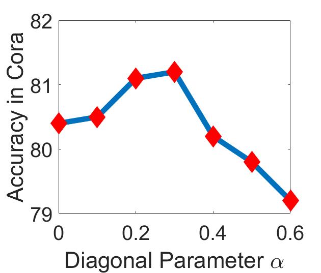
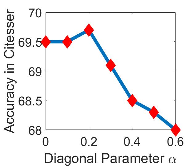
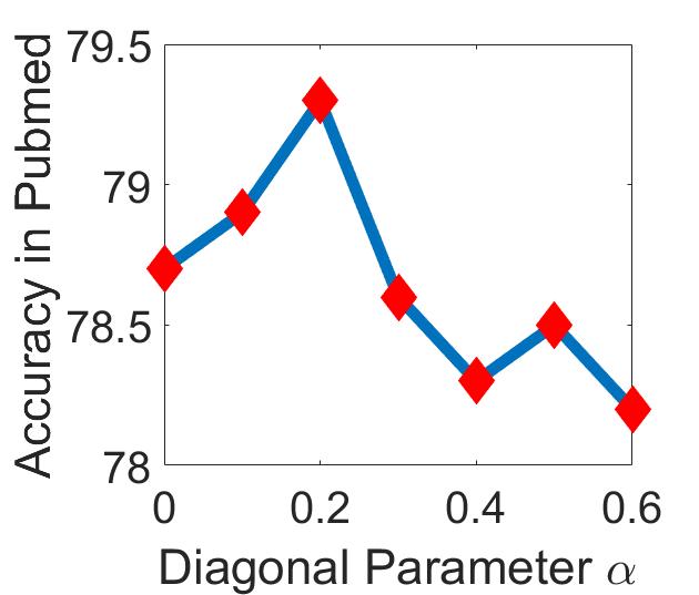
For type-1 first-order TGCN with propagation model , we adjust parameters both manually and automatically. The results are reported in 1 for manual and 2 for automatic adjustments, respectively.
Convolution Layer: For the first-order TGCN, we consider a two-layer structure designed as follows.
| (35) |
where is the specific type of TGCN propgation model, and together with are the parameters of the hidden units. For the higher-order TGCN, we consider a single-layer structure, i.e.,
| (36) |
When training the parameters, we let the neural networks learn the diagonal parameters for type-2 first-order TGCN, and for higher-order TGCN. We applied Adam optimizer [46] for network training. For type-1 first-order TGCN, we apply both manual and automatic adjustments on the diagonal parameters . We train the projection parameter for a variety of TGCNs. For graph representing matrices, we first apply the normalized to measure the effects of layer depth, polynomial orders, and propagation models, respectively. We then test the results of different representing matrices to gain insights and guidelines on how to select suitable graph representations.
Implementation: Let be the set of labeled examples and denote the labels. We evaluate the cross-entropy error over all labeled examples to train parameters, i.e.,
| (37) |
Hyperparameter: For fair comparison of different designs of TGCN, we use the similar hyperparameters, with dropout rate , learning rate and weight decay . For two-layer TGCNs, we let the number of hidden units be . For the higher-order TGCNs, we use fewer hidden units to reduce the complexity.
[b] Num of Layers Polynomial Order TGCN Type Cora Citeseer 2-Layer -order Type-1 81.4 70.1 2-Layer -order Type-2 81.5 70.5 2-Layer -order Type-3 79.5 65.7 2-Layer -order Type-4 79.3 66.9 1-Layer -order Type-1 75.6 67.3 1-Layer -order Type-3 78.4 69.0 1-Layer -order Type-3 79.1 68.4 1-Layer -order Type-4 76.3 67.9 1-Layer -order Type-4 78.6 70.2
-
*
For each method, we test with the representing matrix .
VI-A2 Performances of Different TGCN Propagation Models
We first measure the performances of first-order TGCNs by comparing different propagation models against the traditional GCNs. Note that, the type-1 first-order TGCN degenerates into traditional GCN if the diagonal parameter . To explore the difference between GCN and type-1 first-order TGCN, we adjust the parameter both manually and automatically. The overall accuracy is reported in Table III.
For type-1 first-order TGCN, our manual adjustment results in higher accuracy than automatic adjustment. This indicates that the deep learning network may be more susceptible to local convergence when learning by itself. Usually, the optimal for type-1 TGCN would be in as shown in Fig. 1, while the TGCN degenerates to the traditional GCN for . Generally, type-2 first-order TGCN has a clear advantage in accuracy for all datasets, whereas type-1 frist-order TGCN exhibits only marginal improvement given suitable choice of diagonal parameters.
We then compare different propagation models with different orders of polynomials under the same experiment setup. We start with 100 Monte Carlo random initializations and report the average accuracy of each model in Table IV. The first-order TGCNs generally achieve superior overall accuracy than higher-order TGCNs. Higher-order methods may be occasionally better for some datasets. Recall that the multi-layer first-order TGCN is a special case of single-layer higher-order polynomials as illustrated in Section IV-B. The large number of parameters in the higher-order methods may leads to highly likelihood of overfitting and local convergence, thereby contributing to their less impressive outcomes.
VI-A3 Depth and Polynomial Orders
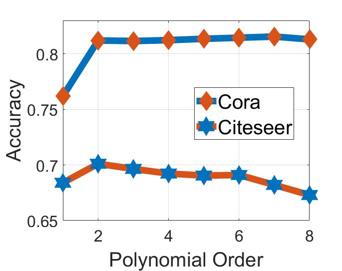
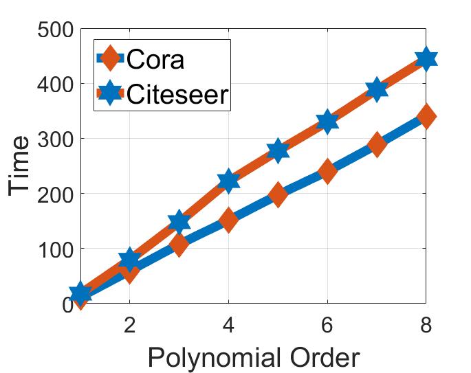
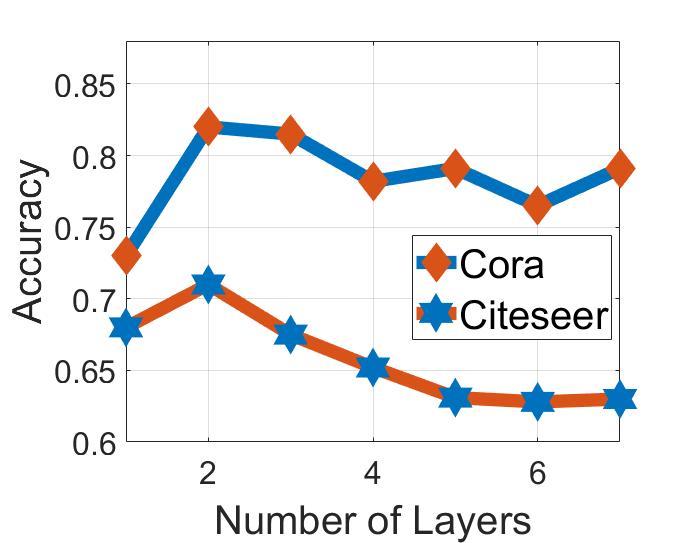
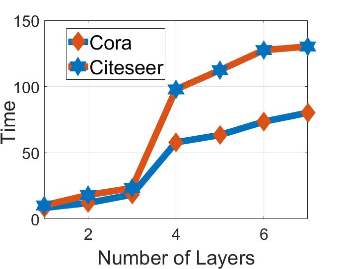
We also test the effects of different polynomial orders and layer numbers. The accuracy and training time (200 epochs) for different polynomial orders (Type-3 as an example) are shown in the first group of plots in Fig. 2. We note that performance improvement appears to saturate beyond certain polynomial order. Since the results also indicate growing training time for higher order polynomials, it would be more efficient to limit the polynomial order to 2 or 3. We also test the performance of first-order TGCNs (Type-2 as an example) with different layers in the last two plots in Fig.2, which also show that a 2-layer or 3-layer TGCN would typically suffice.
VI-A4 Convergence
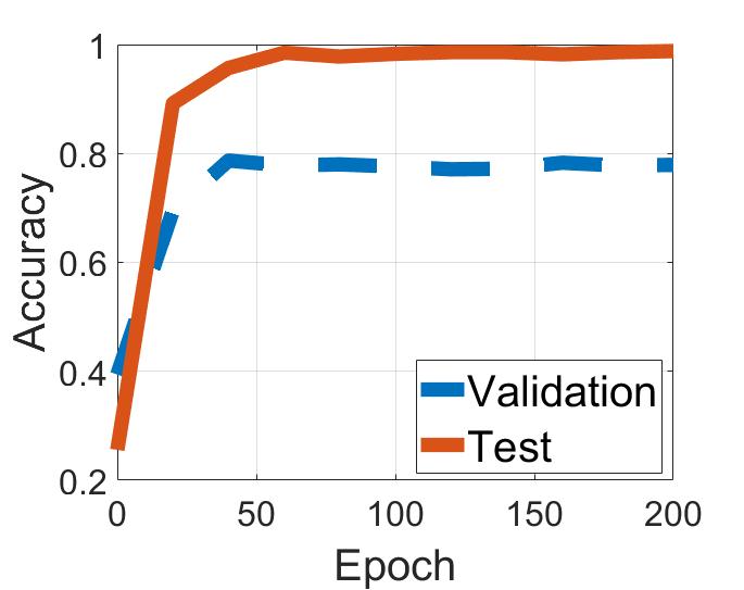
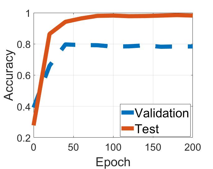
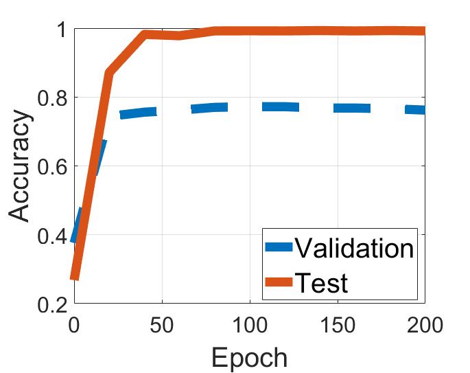
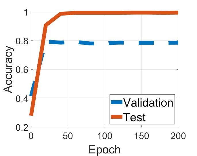
We evaluate the convergence of different TGCN models in Fig. 3. Here, we report the accuracy of training data and validation data for the Cora dataset. Form the results, we can see that TGCN models can converge well in the citation network datasets.
VI-A5 Training Efficiency
[b] Dataset GCN 2L1KT1 2L1KT2 2L2KT3 2L2KT4 Cora 21.2ms 24.3ms 34.0ms 506.1ms 479.5ms Citesser 30.5ms 33.4ms 42.9ms 681.1ms 726.5ms Dataset 1L2KT3 1L3KT3 1L2KT4 1L3KT4 1L1KT1 Cora 253.8ms 463.2ms 244.5ms 641.0ms 11.3ms Citesser 339.3ms 609.7ms 314.7ms 1085.6ms 33.2ms
-
*
Different methods are measured in a CPU-only implementation.
-
*
LKT is short for a Type- TGCN with layers and polynomial order .
We compare the training efficiency for different methods based on the average training time for each epoch over epochs in total. We use the same number of hidden units for multi-layer graph convolutional networks to be fair. From the results of Table V, 2-layer TGCN takes nearly longer than traditional 2-layer GCN because of the larger number of parameters and matrix computations. Moreover, larger layer depth and higher polynomial order also increase TGCN training time.
| Dataset | Cora | Citeseer | Pubmed |
| Type-1 TGCN (2-Layer/Auto-training on ) | |||
| 76.0 | 67.8 | 77.9 | |
| 79.3 | 70.2 | 80.5 | |
| 78.6 | 69.2 | 78.9 | |
| 80.1 | 70.1 | 79.3 | |
| Type-2 TGCN (2-Layer) | |||
| 76.8 | 67.6 | 77.8 | |
| 81.9 | 70.0 | 80.3 | |
| 81.6 | 70.1 | 79.4 | |
| 81.8 | 70.1 | 80.1 | |
| Type-3 TGCN (1-Layer -Order) | |||
| 77.9 | 68.5 | / | |
| 79.0 | 68.9 | / | |
| 78.5 | 69.1 | / | |
| 78.8 | 68.7 | / | |
| Type-4 TGCN (1-Layer -Order) | |||
| 75.2 | 67.0 | / | |
| 79.7 | 68.2 | / | |
| 76.3 | 67.9 | / | |
| 78.3 | 68.0 | / | |
VI-A6 Different Choices of Graph Representations
Thanks to the flexibility of in the TGCN, it is interesting to explore different graph representations in different types of TGCN propagation models. Note that the Laplacian-based model can be written in the form of the adjacency matrix and a corresponding diagonal matrix, which can be included within the category of adjacency-based convolutional propagation models in TGCNs. Thus, we mainly investigate adjacency-based representation for TGCNs. Since there is no constraint on the range of eigenvalues, we test the effect of normalization. More specifically, we use the original adjacency matrix , the normalized adjacency matrix , the traditional GCN propagation , and the pagerank [17]. For the higher-order TGCNs, we mainly focus on Cora and Citeseer datasets due to complexity.
The experiment results are shown in Table VI. The results show that normalized representations exhibit better performance than the unnormalized graph representation for TGCN propagation. More specifically, the normalized adjacency matrix achieves better performance in most TGCN designs. Although the pagerank propagation also shows good performance in some of the TGCN categories, the high-complexity of calculating the inverse matrix is detrimental to its applications in higher-order TGCNs. Note that we only test some of the common graph representations of in our TGCN designs. The Taylor expansions allow a more flexible combination with other existing GCN propagations, such as pagerank and GCN propagations. We plan to further investigate alternative graph representations in future works.
VI-A7 Discussion
In terms of formulation, type-1 TGCN is an extension of GCN, which allows flexible self-influence for each node. Type-2 TGCN is an extension of type-1 TGCN, where different self-influence parameters are assigned for different nodes. In practical applications, such self-influence does exist and may be less obvious. Type-2 TGCN allows different self-influence parameters to be learned while training, which may lead to better performance in the citation networks. Higher-order TGCNs, as discussed in Section IV-B, are different from multi-layer TGCN as various orders may lead to different performances. However, to mitigate complexity concerns, lower-order TGCNs are more efficient in applications. With the steady advances of computation hardware, higher-order TGCNs is expected to play increasingly important roles in future data analysis. In addition, the TGCN designs show a scalable combination with existing GCN propagations and graph representations.
VI-B Comparison with Several Existing Methods
In this section, we compare our proposed TGCNs with several state-of-the-art methods in three different tasks: 1) node classification in the citation network; 2) point cloud segmentation; and 3) classification in synthetic datasets.
| Cora | Citeseer | Pubmed | |
|---|---|---|---|
| GCN | 85.77 | 73.68 | 88.13 |
| GAT | 86.37 | 74.32 | 87.62 |
| GIN | 86.20 | 76.80 | 87.39 |
| Geom-GCN-I | 85.19 | 77.99 | 90.05 |
| Geom-GCN-P | 84.93 | 75.14 | 88.09 |
| Geom-GCN-S | 85.27 | 74.71 | 84.75 |
| APPNP | 86.88 | 77.74 | 88.41 |
| Type-1 TGCN | 86.79 | 77.82 | 87.99 |
| Type-2 TGCN | 87.23 | 78.31 | 86.89 |
VI-B1 Classification in the Citation Networks
We first compare the proposed TGCN frameworks with other GCN-style methods in the citation networks summarized in Table II, but with a different splits on the datasets. Instead of randomly splitting a subset of the citation networks, we apply similar data splits as [33] with 60%/20%/20% for training/testing/validation datasets. We compare our methods with graph convolutional networks (GCN) [1], geometric graph convolutional networks (Geom-GCN) [33], graph attention networks (GAT) [31], approximated personalized propagation of neural predictions (APPNP) [17], and graph isomorphism networks (GIN) [36]. In TGCN propagation, we use the normalized adjacency matrix, i.e., , and set the number of layer to be two. The test results are reported in Table VII. The results show that the proposed TGCN achieves competitive performance against various GCN-type methods. Together with the results presented in Section VI-A, our experiments demonstrate that TGCN is very effective in node classification over the citation graphs despite data splits.
[b] Type-2 TGCN1 Type-1 TGCN1 Type-2 TGCN2 Type-1 TGCN2 GSP HGSP GCN PointNet Airplane 0.7551 0.7883 0.7785 0.7824 0.5272 0.5566 0.7660 0.834 Bag 0.9165 0.9202 0.9399 0.9409 0.5942 0.5620 0.9176 0.787 Cap 0.7670 0.7599 0.7479 0.7577 0.6698 0.7212 0.7629 0.825 Car 0.7114 0.7052 0.7018 0.6976 0.3785 0.3702 0.6790 0.749 Chair 0.6603 0.6197 0.7412 0.6885 0.4701 0.5782 0.6430 0.896 Earphone 0.7037 0.7135 0.7606 0.7712 0.4706 0.5637 0.7054 0.730 Guitar 0.8449 0.8401 0.8176 0.8265 0.5731 0.5889 0.8304 0.915 Knife 0.7675 0.7474 0.7610 0.7614 0.6395 0.7045 0.7502 0.859 Lamp 0.7787 0.7836 0.7853 0.7712 0.2510 0.3112 0.7821 0.808 Laptop 0.8142 0.8365 0.8185 0.8275 0.6704 0.9077 0.8272 0.953 Motorbike 0.7167 0.7183 0.7239 0.7623 0.7663 0.7588 0.7297 0.652 Mug 0.9324 0.9436 0.9348 0.9376 0.7465 0.6290 0.9302 0.930 Pistol 0.7362 0.7387 0.7145 0.7107 0.5336 0.6277 0.7205 0.812 Rocket 0.7895 0.7712 0.7824 0.7742 0.4792 0.5481 0.7807 0.579 Skateboard 0.8323 0.8364 0.8230 0.8493 0.6088 0.5440 0.8176 0.728 Table 0.7984 0.8154 0.7972 0.8194 0.4726 0.4568 0.8164 0.806 Mean 0.7828 0.7836 0.7892 0.7966 0.5532 0.5893 0.7788 0.803
-
1
TGCN1 applies the graph representation .
-
2
TGCN2 applies the graph representation .
-
*
The best graph-based method is marked in bold font.
-
*
The best method is marked in italic script.
VI-B2 Point Cloud Segmentation
We next test the performance of TGCN in the point cloud segmentation. The goal of point cloud segmentation is to identify and cluster points in a point cloud that share similar features into their respective regions [47]. The segmentation problem can be posed as a semi-supervised classification problem if the labels of several samples are known [48].
Datasets and Baselines: In this work, we use the ShapeNet datasets [49, 50] as examples. In this dataset, there are 16 object categories, each of which may contain 2-6 classes. We compare both type-1 and type-2 TGCNs with traditional GCN in all categories. To explore the features extracted from the graph convolution, we also compare the proposed methods with geometric clustering-based methods, including the graph spectral clustering (GSP) and hypergraph spectral clustering (HGSP) [51]. A comparison with a specifically-designed neural networks for point cloud segmentation, i. e., PointNet [52], is also reported.
Experiment Setup:
-
•
To implement TGCN efficiently, we randomly pick 20 point cloud objects from each category, and randomly set points as training data with labels while using the remaining points as the test data for each point cloud. We use -nearest neighbor method to construct an adjacency matrix with elements to indicate the presence or the absence of connection between two nodes , respectively. More specifically, we set in graph construction for all point clouds. For the GCN-like methods, we fix the number of layer as two and the number hidden units as 40 to ensure a fair comparison.
-
•
For the spectral-clustering based methods, we use the hypergraph stationary process [16] to estimate the hypergraph spectrum for the HGSP-based method, and apply the Gaussian distance model [7] to construct the graph for the GSP-based method. The -means clustering is applied for segmentation after obtaining the key spectra.
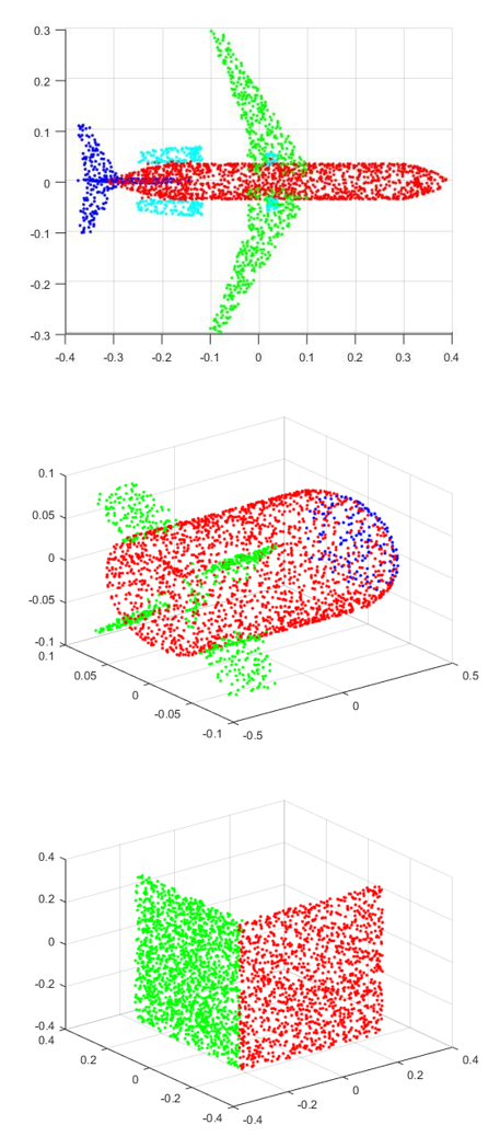
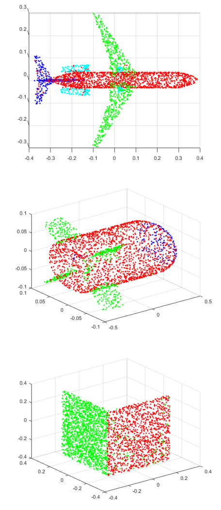
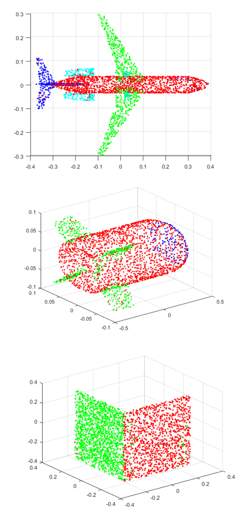
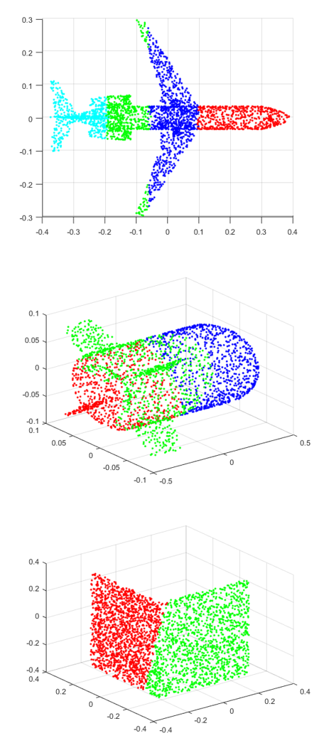
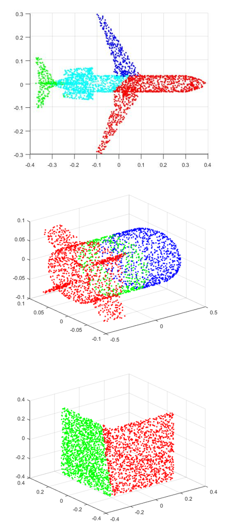
Experiment Results: The overall accuracies of different methods are reported in Table VIII. The resulting mean accuracy of segmentation illustrates that each method under comparison may exhibit some unique strength in different categories. The PointNet exhibits an overall largest mean accuracy, since it is specifically designed for point cloud segmentation while the GCN-like methods are directly applied in classifying the points without adjustment. Even though, the TGCN still shows better performances in some of the categories than PointNet, such as table, skateboard, mug, motorbike, earphone and bag. Compared to the traditional GCN, TGCN generally achieves higher accuracy and provides the better performance in most of the categories. For the graph representation, the normalized adjacency matrix performs better than the traditional GCN propagation matrix in the TGCN designs for point cloud segmentation. The clustering-based methods perform worse than the classification-based methods, since they use no prior knowledge of the ground truth. However, they still achieve satisfying performances in the point clouds with fewer classes and more regular shapes.
To further illustrate different methods, several visualized segmentation results are presented in Fig. 4. Since different TGCN exhibits similar visualized results, we report type-2 TGCN with as an example. From the results, we see that the classification-based methods, i. e., TGCN and GCN, exhibit similar results, where errors are distributed scatteredly over the point clouds. Generally, the TGCN results show fewer errors than those of the traditional GCN, such as in the wings of rockets and planes. Different from GCN-like methods trained according to the ground truth, the clustering-based methods show different results. For example, in the first row of Fig. 4(e), although the segmentation result differ from the ground truth, these results still make sense by grouping two wings to different classes. In addition, the errors of clustering-based methods are grouped together in the intersections of two classes. It will be interesting to explore the integration of classification-based methods and clustering-based methods to extract more features of point clouds in the future works.
| Pattern | Cluster | |||
|---|---|---|---|---|
| Method | Layer | Accuracy | Layer | Accuracy |
| GCN | 4 | 63.88 | 4 | 53.4 |
| GraphSage | 4 | 50.52 | 4 | 68.5 |
| GAT | 4 | 75.84 | 4 | 58.3 |
| GateGCN | 4 | 84.53 | 4 | 60.4 |
| GIN | 4 | 85.59 | 4 | 58.3 |
| RingGNN | 2 | 86.24 | 2 | 42.4 |
| Type-1 TGCN | 4 | 85.43 | 4 | 58.8 |
| Type-2 TGCN | 4 | 85.87 | 4 | 61.2 |
VI-B3 Node Classification in Synthetic Datasets
To provide more comprehensive results of the proposed TGCNs, we also test on the node classification on synthetic datasets following the stochastic block models (SBM), which are widely used to model communities in social networks. We randomly generated SBM graphs with a smaller data size following the similar strategies as [38] with 70%/15%/15% for the training/test/validation. In designing TGCNs, we set the graph representation . An overall result is reported in Table IX. Although the proposed TGCNs do not deliver the top performance in each test case, they are generally robust and competitive across the board.
VII Conclusion
In this work, we explore the inherent connection between GSP convolutional spectrum wavelet and the GCN vertex propagation. Our work shows that spectral wavelet-kernel can be approximated in vertex domain if it admits a polynomial approximation. In addition, we develop an efficient and simple alternative design of GCN layers based on the simple Taylor expansion (TGCN), which exhibits computation efficiency and outperforms a number of state-of-the-art GCN-type methods. Our work derives practial guidelines on the selection of representing matrix and the propagation model for TGCN designs. Our interpretability discussion presents good insights into Taylor approximation of graph convolution.
Future Works: In existing works, the design of GCN centers on performance while neglecting the underlying connection to the original graph spectrum convolution in GSP. Evaluating GCN from the GSP-perspective may provide better insights for layer design and basis for performance analysis in the future. It is equally important for future works to explore the choice of representing matrix and propagation models to further enhance the performance and robustness of GCNs.
References
- [1] T. N. Kipf and M. Welling, “Semi-supervised classification with graph convolutional networks,” in International Conference on Learning Representations (ICLR), Toulon, France, Apr. 2017.
- [2] X. Zhu, Z. Ghahramani, and J. D. Lafferty, “Semi-supervised learning using gaussian fields and harmonic functions,” in Proceedings of the 20th International Conference on Machine learning (ICML-03), Washington DC, USA, Aug. 2003, pp. 912–919.
- [3] S. White and P. Smyth, “A spectral clustering approach to finding communities in graphs,” in Proceedings of the 2005 SIAM International Conference on Data Mining, Newport Beach, CA, USA, 2005, pp. 274–285.
- [4] T. Bühler and M. Hein, “Spectral clustering based on the graph p-laplacian,” in Proceedings of the 26th Annual International Conference on Machine Learning, New York, NY, USA, Jun. 2009, pp. 81–88.
- [5] A. Grover and J. Leskovec, “node2vec: Scalable feature learning for networks,” in Proceedings of the 22nd ACM SIGKDD International Conference on Knowledge Discovery and Data Mining, San Francisco, CA, USA, 2016, pp. 855–864.
- [6] M. Niepert, M. Ahmed, and K. Kutzkov, “Learning convolutional neural networks for graphs,” in International Conference on Machine Learning, New York, NY, USA, Jun. 2016, pp. 2014–2023.
- [7] S. Chen, D. Tian, C. Feng, A. Vetro, and J. Kovačević, “Fast resampling of three-dimensional point clouds via graphs,” IEEE Transactions on Signal Processing, vol. 66, no. 3, pp. 666–681, 2018.
- [8] A. Ortega, P. Frossard, J. Kovačević, J. M. Moura, and P. Vandergheynst, “Graph signal processing: Overview, challenges, and applications,” Proceedings of the IEEE, vol. 106, no. 5, pp. 808–828, May 2018.
- [9] D. I. Shuman, S. K. Narang, P. Frossard, A. Ortega, and P. Vandergheynst, “The emerging field of signal processing on graphs: Extending high-dimensional data analysis to networks and other irregular domains,” IEEE Signal Processing Magazine, vol. 30, no. 3, pp. 83–98, Apr. 2013.
- [10] S. Chen, F. Cerda, P. Rizzo, J. Bielak, J. H. Garrett, and J. Kovačević, “Semi-supervised multiresolution classification using adaptive graph filtering with application to indirect bridge structural health monitoring,” IEEE Transactions on Signal Processing, vol. 62, no. 11, pp. 2879–2893, Jun. 2014.
- [11] Y. Schoenenberger, J. Paratte, and P. Vandergheynst, “Graph-based denoising for time-varying point clouds,” in 2015 3DTV-Conference: The True Vision-Capture, Transmission and Display of 3D Video (3DTV-CON), Lisbon, Portugal, Jul. 2015, pp. 1–4.
- [12] A. Sandryhaila and J. M. Moura, “Discrete signal processing on graphs: Graph filters,” in 2013 IEEE International Conference on Acoustics, Speech and Signal Processing, Vancouver, Canada, May 2013, pp. 6163–6166.
- [13] ——, “Discrete signal processing on graphs: Graph fourier transform,” in 2013 IEEE International Conference on Acoustics, Speech and Signal Processing, Vancouver, Canada, May 2013, pp. 6167–6170.
- [14] D. K. Hammond, P. Vandergheynst, and R. Gribonval, “Wavelets on graphs via spectral graph theory,” Applied and Computational Harmonic Analysis, vol. 30, no. 2, pp. 129–150, Mar. 2011.
- [15] D. I. Shuman, B. Ricaud, and P. Vandergheynst, “A windowed graph fourier transform,” in 2012 IEEE Statistical Signal Processing Workshop (SSP), Ann Arbor, USA, Aug. 2012, pp. 133–136.
- [16] S. Zhang, S. Cui, and Z. Ding, “Hypergraph-based image processing,” in 2020 IEEE International Conference on Image Processing (ICIP), Abu Dhabi, United Arab Emirates, 2020, pp. 216–220.
- [17] J. Klicpera, A. Bojchevski, and S. Günnemann, “Predict then propagate: Graph neural networks meet personalized pagerank,” arXiv preprint arXiv:1810.05997, 2018.
- [18] S. Abu-El-Haija, A. Kapoor, B. Perozzi, and J. Lee, “N-gcn: Multi-scale graph convolution for semi-supervised node classification,” arXiv preprint arXiv:1802.08888, 2018.
- [19] R. Wagner, V. Delouille, and R. Baraniuk, “Distributed wavelet de-noising for sensor networks,” in Proceedings of the 45th IEEE Conference on Decision and Control, San Diego, CA, USA, Dec. 2006, pp. 373–379.
- [20] S. K. Narang and A. Ortega, “Local two-channel critically sampled filter-banks on graphs,” in 2010 IEEE International Conference on Image Processing, Hong Kong, China, Jan. 2010, pp. 333–336.
- [21] X. Zhu and M. Rabbat, “Approximating signals supported on graphs,” in 2012 IEEE International Conference on Acoustics, Speech and Signal Processing (ICASSP), Japan, Mar. 2012, pp. 3921–3924.
- [22] S. Chen, R. Varma, A. Sandryhaila, and J. Kovačević, “Discrete signal processing on graphs: sampling theory,” IEEE Transactions on Signal Processing, vol. 63, no. 24, pp. 6510–6523, Dec. 2015.
- [23] A. Sandryhaila and J. M. Moura, “Discrete signal processing on graphs: Frequency analysis,” IEEE Transactions on Signal Processing, vol. 62, no. 12, pp. 3042–3054, Apr. 2014.
- [24] A. G. Marques, S. Segarra, G. Leus, and A. Ribeiro, “Stationary graph processes and spectral estimation,” IEEE Transactions on Signal Processing, vol. 65, no. 22, pp. 5911–5926, Aug. 2017.
- [25] S. Zhang, Z. Ding, and S. Cui, “Introducing hypergraph signal processing: Theoretical foundation and practical applications,” IEEE Internet of Things Journal, vol. 7, no. 1, Jan. 2020.
- [26] S. Barbarossa and S. Sardellitti, “Topological signal processing over simplicial complexes,” IEEE Transactions on Signal Processing, Mar. 2020.
- [27] L. Page, S. Brin, R. Motwani, and T. Winograd, “The pagerank citation ranking: Bringing order to the web.” Stanford InfoLab, Tech. Rep., 1999.
- [28] X. Bresson and T. Laurent, “Residual gated graph convnets,” arXiv preprint arXiv:1711.07553, 2017.
- [29] W. Hamilton, Z. Ying, and J. Leskovec, “Inductive representation learning on large graphs,” in Advances in Neural Information Processing Systems, Long Beach, USA, Dec. 2017, pp. 1024–1034.
- [30] F. Monti, D. Boscaini, J. Masci, E. Rodola, J. Svoboda, and M. M. Bronstein, “Geometric deep learning on graphs and manifolds using mixture model cnns,” in Proceedings of the IEEE Conference on Computer Vision and Pattern Recognition, Hawaii, USA, Jul. 2017, pp. 5115–5124.
- [31] P. Veličković, G. Cucurull, A. Casanova, A. Romero, P. Lio, and Y. Bengio, “Graph attention networks,” arXiv preprint arXiv:1710.10903, 2017.
- [32] Z. Ying, J. You, C. Morris, X. Ren, W. Hamilton, and J. Leskovec, “Hierarchical graph representation learning with differentiable pooling,” in Advances in Neural Information Processing Systems, Montreal, Canada, Dec. 2018, pp. 4800–4810.
- [33] H. Pei, B. Wei, K. C.-C. Chang, Y. Lei, and B. Yang, “Geom-gcn: Geometric graph convolutional networks,” arXiv preprint arXiv:2002.05287, 2020.
- [34] S. Abu-El-Haija, B. Perozzi, A. Kapoor, N. Alipourfard, K. Lerman, H. Harutyunyan, G. V. Steeg, and A. Galstyan, “Mixhop: Higher-order graph convolutional architectures via sparsified neighborhood mixing,” arXiv preprint arXiv:1905.00067, 2019.
- [35] J. Atwood and D. Towsley, “Diffusion-convolutional neural networks,” in Advances in Neural Information Processing Systems, 2016, pp. 1993–2001.
- [36] K. Xu, W. Hu, J. Leskovec, and S. Jegelka, “How powerful are graph neural networks?” arXiv preprint arXiv:1810.00826, 2018.
- [37] M. M. Bronstein, J. Bruna, Y. LeCun, A. Szlam, and P. Vandergheynst, “Geometric deep learning: going beyond euclidean data,” IEEE Signal Processing Magazine, vol. 34, no. 4, pp. 18–42, Jul. 2017.
- [38] V. P. Dwivedi, C. K. Joshi, T. Laurent, Y. Bengio, and X. Bresson, “Benchmarking graph neural networks,” arXiv preprint arXiv:2003.00982, 2020.
- [39] J. Shi and J. M. Moura, “Graph signal processing: Modulation, convolution, and sampling,” arXiv preprint arXiv:1912.06762, 2019.
- [40] J. Pons, J. Miralles, and J. M. Ibáñez, “Legendre expansion of the kernel: Influence of high order terms,” Astronomy and Astrophysics Supplement Series, vol. 129, no. 2, pp. 343–351, 1998.
- [41] S. Linnainmaa, “Taylor expansion of the accumulated rounding error,” BIT Numerical Mathematics, vol. 16, no. 2, pp. 146–160, 1976.
- [42] A. K. McCallum, K. Nigam, J. Rennie, and K. Seymore, “Automating the construction of internet portals with machine learning,” Information Retrieval, vol. 3, no. 2, pp. 127–163, Jul. 2000.
- [43] A. Bojchevski and S. Günnemann, “Deep gaussian embedding of graphs: Unsupervised inductive learning via ranking,” arXiv preprint arXiv:1707.03815, 2017.
- [44] P. Sen, G. Namata, M. Bilgic, L. Getoor, B. Galligher, and T. Eliassi-Rad, “Collective classification in network data,” AI magazine, vol. 29, no. 3, pp. 93–93, 2008.
- [45] G. Namata, B. London, L. Getoor, B. Huang, and U. EDU, “Query-driven active surveying for collective classification,” in 10th International Workshop on Mining and Learning with Graphs, vol. 8, Edinburgh, Scotland, Jul. 2012.
- [46] D. P. Kingma and J. Ba, “Adam: A method for stochastic optimization,” arXiv preprint arXiv:1412.6980, 2014.
- [47] A. Nguyen and B. Le, “3d point cloud segmentation: A survey,” in 2013 6th IEEE Conference on Robotics, Automation and Mechatronics (RAM), Manila, Philippines, Nov. 2013, pp. 225–230.
- [48] J. Lv, X. Chen, J. Huang, and H. Bao, “Semi-supervised mesh segmentation and labeling,” in Computer Graphics Forum, vol. 31, no. 7. Wiley Online Library, 2012, pp. 2241–2248.
- [49] A. X. Chang, T. Funkhouser, L. Guibas, P. Hanrahan, Q. Huang, Z. Li, S. Savarese, M. Savva, S. Song, H. Su et al., “Shapenet: An information-rich 3d model repository,” arXiv preprint arXiv:1512.03012, 2015.
- [50] L. Yi, L. Shao, M. Savva, H. Huang, Y. Zhou, Q. Wang, B. Graham, M. Engelcke, R. Klokov, V. Lempitsky et al., “Large-scale 3d shape reconstruction and segmentation from shapenet core55,” arXiv preprint arXiv:1710.06104, 2017.
- [51] S. Zhang, S. Cui, and Z. Ding, “Hypergraph spectral clustering for point cloud segmentation,” IEEE Signal Processing Letters, vol. 27, pp. 1655–1659, 2020.
- [52] C. R. Qi, H. Su, K. Mo, and L. J. Guibas, “Pointnet: Deep learning on point sets for 3d classification and segmentation,” in Proceedings of the IEEE Conference on Computer Vision and Pattern Recognition, 2017, pp. 652–660.