Bayesian Coresets:
Revisiting the Nonconvex Optimization Perspective


Jacky Y. Zhang1                        Rajiv Khanna2                        Anastasios Kyrillidis3                        Oluwasanmi Koyejo1 yiboz@illinois.edu         rajivak@berkeley.edu         anastasios@rice.edu         sanmi@illinois.edu 1University of Illinois at Urbana-Champaign        2University of California, Berkeley        3Rice University

Abstract

Bayesian coresets have emerged as a promising approach for implementing scalable Bayesian inference. The Bayesian coreset problem involves selecting a (weighted) subset of the data samples, such that the posterior inference using the selected subset closely approximates the posterior inference using the full dataset. This manuscript revisits Bayesian coresets through the lens of sparsity constrained optimization. Leveraging recent advances in accelerated optimization methods, we propose and analyze a novel algorithm for coreset selection. We provide explicit convergence rate guarantees and present an empirical evaluation on a variety of benchmark datasets to highlight our proposed algorithm’s superior performance compared to state-of-the-art on speed and accuracy.

1 Introduction

Bayesian coresets have emerged as a promising approach for scalable Bayesian inference (Huggins et al., 2016; Campbell & Broderick, 2018, 2019; Campbell & Beronov, 2019). The key idea is to select a (weighted) subset of the data such that the posterior inference using the selected subset closely approximates the posterior inference using the full dataset. This creates a trade-off, where using Bayesian coresets as opposed to the full dataset exchanges approximation accuracy for computational speedups. We study Bayesian coresets as they are easy to implement, effective in practice, and come with useful theoretical guarantees that relate the coreset size with the approximation quality.

The main technical challenge in the Bayesian coreset problem lies in handling the combinatorial constraints – we desire to select a few data points out of many as the coreset. In terms of optimization, previous approaches mainly rely on two ideas: convexification and greedy methods. In convexification (Campbell & Broderick, 2019), the sparsity constraint – i.e., selection of k𝑘k data samples – is relaxed into a convex 1subscript1\ell_{1}-norm constraint. This allows them to use out-of-the-box solvers such as Frank-Wolfe (FW) type-of methods (Frank & Wolfe, 1956; Jaggi, 2013). An alternative approach is by using greedy methods (Campbell & Broderick, 2018), which constructs a sparse weight vector based on local decisions to greedily optimize the approximation problem (Tropp & Gilbert, 2007; Needell & Tropp, 2009). The resulting method, greedy iterative geodesic ascent (GIGA), achieves linear convergence with no hyper-parameter tuning and optimal scaling (Campbell & Broderick, 2018). More recently, sparse variational inference (SparseVI) is considered for Bayesian coreset construction. SparseVI also employs a greedy algorithm to minimize a KL divergence objective. The method achieves state-of-the-art accuracy, but at a cost of higher computational requirements. Therefore, existing work illustrates the trade-off between accuracy and efficiency, opening a gap for improvements.

We revisit Bayesian coresets through the lens of sparsity constrained optimization. Sparsity, a kind of nonconvexity, appears in a variety of applications in machine learning and statistics. For instance, compressed sensing (Donoho et al., 2006; Candes, 2008) is an example where sparsity is used as a complexity measure for signal representation. Leveraging and building upon recent advances in non-convex optimization, we solve the Bayesian coreset problem based on hard thresholding algorithms (Blumensath & Davies, 2009) that directly work on the non-convex sparsity constraint. Hard-thresholding schemes are highly flexible, and easily accommodate variations such as subspace exploration (Dai & Milenkovic, 2009), de-bias steps (Needell & Tropp, 2009), adaptive step size selections (Kyrillidis & Cevher, 2011), as well as different types of sparsity constraints, such as group sparsity (Baldassarre et al., 2016), sparsity within groups (Kyrillidis et al., 2015), and generic structured sparsity (Baraniuk et al., 2010). The thresholding step involves a projection onto the k𝑘k-sparsity constraint set to determine the selected sample set in each iteration. While we achieve state-of-the-art accuracy using direct application of this algorithm, re-building the set in every iteration makes it slower than previous works. To fix this, we employ line search for step size selection and momentum based techniques (Khanna & Kyrillidis, 2018) to accelerate the algorithm, also achieving state-of-the-art speed.

Contributions. In this paper, we adapt accelerated iterative hard thresholding schemes to the Bayesian coreset problem. Despite directly attacking the non-convex optimization problem, we provide strong convergence guarantees. To summarize our contributions:

  • We revisit the Bayesian coreset problem via a non-convex (sparse) optimization lens, and provide an IHT-based algorithm that combines hard thresholding and momentum steps;

  • We analyze its convergence based on standard assumptions;

  • We provide extensive empirical evaluation111Code available at https://github.com/jackyzyb/bayesian-coresets-optimization to show superior performance of the proposed method vis-à-vis state-of-the-art algorithms in terms of approximation accuracy as well as speed.

2 Problem Formulation

Given n𝑛n observations, one can compute the log-likelihood i(θ)subscript𝑖𝜃{\mathcal{L}}_{i}(\theta) of each of the observations, parameterized by θ𝜃\theta. Assuming observations are conditionally independent given θ𝜃\theta, one can represent the likelihood of all the observations as the sum of individual log-likelihoods, i.e., (θ)=i=1ni(θ)𝜃superscriptsubscript𝑖1𝑛subscript𝑖𝜃{\mathcal{L}}(\theta)=\sum_{i=1}^{n}{\mathcal{L}}_{i}(\theta). With prior density π0(θ)subscript𝜋0𝜃\pi_{0}(\theta), the posterior density can be derived as:

π(θ):=1Z\displaystyle\pi(\theta):=\tfrac{1}{Z}\cdot e(θ)π0(θ),superscript𝑒𝜃subscript𝜋0𝜃\displaystyle e^{{\mathcal{L}}(\theta)}\cdot\pi_{0}(\theta), (1)

where Z=e(θ)π0(θ)𝑑θ𝑍superscript𝑒𝜃subscript𝜋0𝜃differential-d𝜃Z=\int e^{{\mathcal{L}}(\theta)}\pi_{0}(\theta)d\theta is a normalization factor.

However, for most applications, exact posterior estimation is intractable; i.e., π𝜋\pi is too hard to evaluate exactly. Practitioners use algorithms for approximate inference that may approximate the π𝜋\pi in a closed-form (e.g., using variational inference), or allow for sampling from the posterior without providing a closed-form expression (e.g., MCMC methods). Such algorithms often scale at least linearly with the size of the dataset n𝑛n, which makes them prohibitively expensive for large datasets. As such, designing algorithms to speed up inference is an area of active research.

One solution to the scalability problem is to use coresets. Coresets approximate the empirical log-likelihood =i=1nisuperscriptsubscript𝑖1𝑛subscript𝑖{\mathcal{L}}=\sum_{i=1}^{n}{\mathcal{L}}_{i} using a weighted sum of a subset of all the log-likelihoods isubscript𝑖{\mathcal{L}}_{i}. In other words, we use w=i=1nwiisubscript𝑤superscriptsubscript𝑖1𝑛subscript𝑤𝑖subscript𝑖{\mathcal{L}}_{w}=\sum_{i=1}^{n}w_{i}{\mathcal{L}}_{i} to approximate the true {\mathcal{L}}, where w+n𝑤superscriptsubscript𝑛w\in\mathbb{R}_{+}^{n} is a non-negative sparse vector. It will be useful to view that ,isubscript𝑖{\mathcal{L}},{\mathcal{L}}_{i} and wsubscript𝑤{\mathcal{L}}_{w} are functions in a Hilbert space, and we will use L2superscript𝐿2L^{2}-norm to denote the 2-norm defined in function space, differentiating with the 2subscript2\ell_{2}-norm defined in Euclidean space. We enforce the sparsity constraint as w0ksubscriptnorm𝑤0𝑘\|w\|_{0}\leq k, for k<n𝑘𝑛k<n; here 0\|\cdot\|_{0} denotes the pseudo-norm that counts the number of non-zero entries.

When k<n𝑘𝑛k<n, posterior estimation (e.g., using MCMC or variational inference) is less expensive on the coreset as opposed to the entire dataset. However, sparsifying w𝑤w involves dropping some samples, which in turn implies deviating from the best performance possible from using the full dataset. The Bayesian coreset problem is formulated to minimize this loss in performance.

The Bayesian Coreset Problem. The Bayesian coreset problem is to control the deviation of coreset log-likelihood from true log-likelihood via sparsity:

argminwn𝑤superscript𝑛argmin\displaystyle\underset{w\in\mathbb{R}^{n}}{\operatorname*{arg\,min}} f(w):=Dist(,w)assign𝑓𝑤Distsubscript𝑤\displaystyle f(w):=\textsc{Dist}(\mathcal{L},\;\mathcal{L}_{w}) (2)
      s.t. w0k,wi0,i.formulae-sequencesubscriptnorm𝑤0𝑘subscript𝑤𝑖0for-all𝑖\displaystyle\|w\|_{0}\leq k,\;w_{i}\geq 0,\forall i.\vspace{-0.1cm}

Key components are (i)𝑖(i) the weights w+n𝑤superscriptsubscript𝑛w\in\mathbb{R}_{+}^{n} over n𝑛n data points, (ii)𝑖𝑖(ii) the function f()𝑓f(\cdot) that controls the deviation between the full-dataset log-likelihood \mathcal{L} and the coreset log-likelihood wsubscript𝑤\mathcal{L}_{w} using the distance functional Dist(,)Dist\textsc{Dist}(\cdot,\;\cdot), and (iii)𝑖𝑖𝑖(iii) the non-convex sparsity constraint that restricts the number of nonzeros in w𝑤w, thus constraining the number of active data points in the coreset. Examples of Dist(,)Dist\textsc{Dist}(\cdot,\;\cdot) include the weighted L2superscript𝐿2L^{2}-norm (Campbell & Broderick, 2019) and the KL-divergence (Campbell & Beronov, 2019). In this manuscript, we consider the L2(π^)superscript𝐿2^𝜋L^{2}(\hat{\pi})-norm as the distance metric in the embedding Hilbert space, i.e.,

Dist(,w)2Distsuperscriptsubscript𝑤2\displaystyle\textsc{Dist}(\mathcal{L},\;\mathcal{L}_{w})^{2} =wπ^,22absentsubscriptsuperscriptnormsubscript𝑤2^𝜋2\displaystyle=\|\mathcal{L}-\mathcal{L}_{w}\|^{2}_{\hat{\pi},2} (3)
=𝔼θπ^[((θ)w(θ))2],absentsubscript𝔼similar-to𝜃^𝜋delimited-[]superscript𝜃subscript𝑤𝜃2\displaystyle=\mathbb{E}_{\theta\sim\hat{\pi}}\left[(\mathcal{L}(\theta)-\mathcal{L}_{w}(\theta))^{2}\right], (4)

where π^^𝜋\hat{\pi} is a weighting distribution that has the same support as true posterior π𝜋\pi. Ideally, π^^𝜋\hat{\pi} is the true posterior, which is obviously unknown. However, one can employ Laplace approximation to derive an inexpensive and reasonable approximation for π^^𝜋\hat{\pi} (Campbell & Broderick, 2019).

To account for the shift invariance, we write gi=i𝔼θπ^i(θ)subscript𝑔𝑖subscript𝑖subscript𝔼similar-to𝜃^𝜋subscript𝑖𝜃g_{i}={\mathcal{L}}_{i}-\mathbb{E}_{\theta\sim\hat{\pi}}{\mathcal{L}}_{i}(\theta), so the equivalent optimization problem is now: minimize i=1ngii=1nwigiπ^,22subscriptsuperscriptnormsuperscriptsubscript𝑖1𝑛subscript𝑔𝑖superscriptsubscript𝑖1𝑛subscript𝑤𝑖subscript𝑔𝑖2^𝜋2\|\sum_{i=1}^{n}g_{i}-\sum_{i=1}^{n}w_{i}g_{i}\|^{2}_{\hat{\pi},2}. Further, noting that the L2(π^)superscript𝐿2^𝜋L^{2}(\hat{\pi})-norm is in the form of expectation (equation (4)), it can be approximated by a finite-dimensional 2subscript2\ell_{2}-norm which replaces the function with a vector of sampled evaluations θπ^similar-to𝜃^𝜋\theta\sim\hat{\pi}, i.e., its Monte Carlo approximation. Thus, given S𝑆S samples {θj}j=1S,θjπ^similar-tosuperscriptsubscriptsubscript𝜃𝑗𝑗1𝑆subscript𝜃𝑗^𝜋\{\theta_{j}\}_{j=1}^{S},\theta_{j}\sim\hat{\pi}, and using

g^i=1S[i(θ1)i¯,,i(θS)i¯]Ssubscript^𝑔𝑖1𝑆superscriptsubscript𝑖subscript𝜃1¯subscript𝑖subscript𝑖subscript𝜃𝑆¯subscript𝑖topsuperscript𝑆\hat{g}_{i}=\tfrac{1}{\sqrt{S}}\cdot\left[{\mathcal{L}}_{i}(\theta_{1})-\bar{{\mathcal{L}}_{i}},\dots,{\mathcal{L}}_{i}(\theta_{S})-\bar{{\mathcal{L}}_{i}}\right]^{\top}\in\mathbb{R}^{S}

as projections from function space to standard Euclidean space, where i¯=1Sj=1Si(θj)¯subscript𝑖1𝑆superscriptsubscript𝑗1𝑆subscript𝑖subscript𝜃𝑗\bar{{\mathcal{L}}_{i}}=\frac{1}{S}\sum_{j=1}^{S}{\mathcal{L}}_{i}(\theta_{j}), the Bayesian coreset problem (2) becomes a finite-dimensional sparse regression problem:

argminwnf(w):=i=1ng^ii=1nwig^i22 s.t. w0k,wi0,i.missing-subexpressionassign𝑤superscript𝑛𝑓𝑤superscriptsubscriptnormsuperscriptsubscript𝑖1𝑛subscript^𝑔𝑖superscriptsubscript𝑖1𝑛subscript𝑤𝑖subscript^𝑔𝑖22missing-subexpressionformulae-sequence s.t. subscriptnorm𝑤0𝑘subscript𝑤𝑖0for-all𝑖\displaystyle\begin{aligned} &\underset{w\in\mathbb{R}^{n}}{\arg\min}\quad f(w):=\left\|\sum_{i=1}^{n}\hat{g}_{i}-\sum_{i=1}^{n}w_{i}\hat{g}_{i}\right\|_{2}^{2}\\ &\quad\text{ s.t. }\quad\|w\|_{0}\leq k,\quad w_{i}\geq 0,\forall i.\end{aligned} (5)

The resulting sparse regression problem is non-convex due to the combinatorial nature of the constraints. Previous methods that use this 2subscript2\ell_{2}-norm formulation (Campbell & Broderick, 2019, 2018) offers less satisfactory approximation accuracy compared to the state-of-the-art sparse variational inference method (Campbell & Beronov, 2019). However, the high computational cost of the latter method makes it impractical for real-world large datasets. Nonetheless, as we will show, our approach for solving equation (5) using a variant of iterative hard thresholding, achieves better accuracy and speed.

3 Our approach

0:  Objective f:n:𝑓superscript𝑛f:\mathbb{R}^{n}\to\mathbb{R}; sparsity k𝑘k; step size μ𝜇\mu
1:  Initialize w𝑤w
2:  repeat
3:     wΠ𝒞k+n(wμf(w))𝑤subscriptΠsubscript𝒞𝑘subscriptsuperscript𝑛𝑤𝜇𝑓𝑤w\leftarrow\Pi_{\mathcal{C}_{k}\cap{\mathbb{R}}^{n}_{+}}\left(w-\mu\nabla f(w)\right)
4:  until Stop criteria met
5:  return w𝑤w
Algorithm 1 Vanilla IHT

For clarity of exposition, we gradually build up our approach for solving the optimization problem (5). The fundamental ingredient of our approach is the vanilla Iterative Hard Thresholding (IHT) method presented in Algorithm 1. We develop our approach by augmenting IHT with momentum updates, step size selection for line search and active subspace expansion techniques to accelerate and automate the algorithm (Algorithms 23). Details follow.

3.1 Iterative Hard Thresholding (IHT)

The classical IHT (Blumensath & Davies, 2009) is a projected gradient descent method that performs a gradient descent step and then projects the iterate onto the non-convex k𝑘k-sparsity constraint set. We denote the orthogonal projection of a given zn𝑧superscript𝑛z\in\mathbb{R}^{n} to a space 𝒞n𝒞superscript𝑛\mathcal{C}\subseteq\mathbb{R}^{n} as: Π𝒞(z):=argminw𝒞wz2assignsubscriptΠ𝒞𝑧subscriptargmin𝑤𝒞subscriptnorm𝑤𝑧2\Pi_{\mathcal{C}}(z):=\operatorname*{arg\,min}_{w\in\mathcal{C}}\|w-z\|_{2}. Define the sparsity restricted space as: 𝒞k={wn:|supp(w)|k}subscript𝒞𝑘conditional-set𝑤superscript𝑛supp𝑤𝑘\mathcal{C}_{k}=\big{\{}w\in\mathbb{R}^{n}:\left|\text{supp}(w)\right|\leq k\big{\}}, where supp(w)={i|wi0}supp𝑤conditional-set𝑖subscript𝑤𝑖0\text{supp}(w)=\{i|w_{i}\neq 0\} denotes the support set of w𝑤w. Here, we describe the plain sparsity case, but one can consider different realizations of 𝒞ksubscript𝒞𝑘\mathcal{C}_{k} as in (Baldassarre et al., 2016; Kyrillidis et al., 2015; Baraniuk et al., 2010). The projection step in the classical IHT, i.e.,, Π𝒞ksubscriptΠsubscript𝒞𝑘\Pi_{{\mathcal{C}}_{k}}, can be computed easily by selecting the top-k𝑘k elements in O(nlogk)𝑂𝑛𝑘O(n\log k) time; but projection can be more challenging for more complex constraint sets, e.g., if the variable is a distribution on a lattice (Zhang et al., 2019).

For our problem, we require that the projected sparse vector only has non-negative values. For vector variate functions, the projection step in Algorithm 1, i.e., Π𝒞k+n(w)subscriptΠsubscript𝒞𝑘subscriptsuperscript𝑛𝑤\Pi_{\mathcal{C}_{k}\cap\mathbb{R}^{n}_{+}}(w) is also straightforward; it can be done optimally in O(nlogk)𝑂𝑛𝑘O(n\log k) time by simply picking the top k𝑘k largest non-negative elements. More discussions about the projections are presented in section B in appendix.

3.2 Accelerated IHT

For clarity, we rewrite the problem in equation (5) as:

w=argminw𝒞k+nf(w):=yΦw22,formulae-sequencesuperscript𝑤subscriptargmin𝑤subscript𝒞𝑘subscriptsuperscript𝑛assign𝑓𝑤superscriptsubscriptnorm𝑦Φ𝑤22\displaystyle w^{*}=\operatorname*{arg\,min}_{w\in\mathcal{C}_{k}\cap\mathbb{R}^{n}_{+}}\quad f(w):=\|y-\Phi w\|_{2}^{2}, (6)

where y=i=1ng^i𝑦superscriptsubscript𝑖1𝑛subscript^𝑔𝑖y=\sum_{i=1}^{n}\hat{g}_{i} and Φ=[g^1,,g^n]Φsubscript^𝑔1subscript^𝑔𝑛\Phi=[\hat{g}_{1},\dots,\hat{g}_{n}]. In this case, f(w)2Φ(yΦw)𝑓𝑤2superscriptΦtop𝑦Φ𝑤\nabla f(w)\equiv-2\Phi^{\top}(y-\Phi w).

Step size selection in IHT: Classical results on the performance of IHT algorithms come with rigorous convergence guarantees (under regularity conditions) (Blumensath & Davies, 2009; Foucart, 2011). However, these results require step size assumptions that either do not work in practice, or rely on strong assumptions. For example, in (Blumensath & Davies, 2009; Foucart, 2011) strong isometry constant bounds are assumed to allow step size μ=1𝜇1\mu=1 for all the iterations, and thus remove the requirement of hyper-parameter tuning. Moreover, the authors in (Blumensath & Davies, 2010) present toy examples by carefully selecting ΦΦ\Phi so that the vanilla IHT algorithm diverges without appropriate step size selection. In this work, given the quadratic objective f(w)𝑓𝑤f(w), we perform exact line search to obtain the best step size per iteration (Blumensath & Davies, 2010; Kyrillidis & Cevher, 2011): μt:=~t22/2Φ~t22assignsubscript𝜇𝑡superscriptsubscriptnormsubscript~𝑡222subscriptsuperscriptnormΦsubscript~𝑡22\mu_{t}:=\|\widetilde{\nabla}_{t}\|_{2}^{2}/2\|\Phi\widetilde{\nabla}_{t}\|^{2}_{2}; details in Algorithm 2.

Algorithm 2 Automated Accelerated IHT (A-IHT)
0:  Objective f(w)=yΦw22𝑓𝑤superscriptsubscriptnorm𝑦Φ𝑤22f(w)=\|y-\Phi w\|_{2}^{2}; sparsity k𝑘k
1:  t=0𝑡0t=0, z0=0subscript𝑧00z_{0}=0, w0=0subscript𝑤00w_{0}=0
2:  repeat
3:     𝒵=supp(zt)𝒵suppsubscript𝑧𝑡\mathcal{Z}=\text{supp}(z_{t})
4:     𝒮=supp(Π𝒞k𝒵(f(zt)))𝒵𝒮suppsubscriptΠsubscript𝒞𝑘𝒵𝑓subscript𝑧𝑡𝒵\mathcal{S}=\text{supp}(\Pi_{\mathcal{C}_{k}\setminus\mathcal{Z}}\left(\nabla f(z_{t})\right))\cup\mathcal{Z} where |𝒮|3k𝒮3𝑘|\mathcal{S}|\leq 3k
5:     ~t=f(zt)|𝒮subscript~𝑡evaluated-at𝑓subscript𝑧𝑡𝒮\widetilde{\nabla}_{t}=\nabla f(z_{t})\big{|}_{\mathcal{S}}
6:     μt=argminμf(ztμ~t)=~t222Φ~t22subscript𝜇𝑡subscriptargmin𝜇𝑓subscript𝑧𝑡𝜇subscript~𝑡superscriptsubscriptnormsubscript~𝑡222subscriptsuperscriptnormΦsubscript~𝑡22\mu_{t}=\operatorname*{arg\,min}_{\mu}f(z_{t}-\mu\widetilde{\nabla}_{t})=\frac{\|\widetilde{\nabla}_{t}\|_{2}^{2}}{2\|\Phi\widetilde{\nabla}_{t}\|^{2}_{2}}
7:     wt+1=Π𝒞k+n(ztμtf(zt))subscript𝑤𝑡1subscriptΠsubscript𝒞𝑘subscriptsuperscript𝑛subscript𝑧𝑡subscript𝜇𝑡𝑓subscript𝑧𝑡w_{t+1}=\Pi_{\mathcal{C}_{k}\cap\mathbb{R}^{n}_{+}}\left(z_{t}-\mu_{t}\nabla f(z_{t})\right)
8:     τt+1=argminτf(wt+1+τ(wt+1wt))subscript𝜏𝑡1subscriptargmin𝜏𝑓subscript𝑤𝑡1𝜏subscript𝑤𝑡1subscript𝑤𝑡\tau_{t+1}=\operatorname*{arg\,min}_{\tau}f(w_{t+1}+\tau(w_{t+1}-w_{t}))    =yΦwt+1,Φ(wt+1wt)2Φ(wt+1wt)22absent𝑦Φsubscript𝑤𝑡1Φsubscript𝑤𝑡1subscript𝑤𝑡2subscriptsuperscriptnormΦsubscript𝑤𝑡1subscript𝑤𝑡22=\frac{\langle y-\Phi w_{t+1},\Phi(w_{t+1}-w_{t})\rangle}{2\|\Phi(w_{t+1}-w_{t})\|^{2}_{2}}
9:     zt+1=wt+1+τt+1(wt+1wt)subscript𝑧𝑡1subscript𝑤𝑡1subscript𝜏𝑡1subscript𝑤𝑡1subscript𝑤𝑡z_{t+1}=w_{t+1}+\tau_{t+1}(w_{t+1}-w_{t})
10:     t=t+1𝑡𝑡1t=t+1
11:  until Stop criteria met
12:  return wtsubscript𝑤𝑡w_{t}

Memory in vanilla IHT: Based upon the same ideas as step size selection, we propose to include adaptive momentum acceleration; we select the momentum term as the minimizer of the objective: τt+1=argminτf(wt+1+τ(wt+1wt))=yΦwt+1,Φ(wt+1wt)2Φ(wt+1wt)22subscript𝜏𝑡1subscriptargmin𝜏𝑓subscript𝑤𝑡1𝜏subscript𝑤𝑡1subscript𝑤𝑡𝑦Φsubscript𝑤𝑡1Φsubscript𝑤𝑡1subscript𝑤𝑡2subscriptsuperscriptnormΦsubscript𝑤𝑡1subscript𝑤𝑡22\tau_{t+1}=\operatorname*{arg\,min}_{\tau}f(w_{t+1}+\tau(w_{t+1}-w_{t}))=\frac{\langle y-\Phi w_{t+1},\Phi(w_{t+1}-w_{t})\rangle}{2\|\Phi(w_{t+1}-w_{t})\|^{2}_{2}}, which also comes out as a closed-form solution. The step zt+1=wt+1+τt+1(wt+1wt)subscript𝑧𝑡1subscript𝑤𝑡1subscript𝜏𝑡1subscript𝑤𝑡1subscript𝑤𝑡z_{t+1}=w_{t+1}+\tau_{t+1}(w_{t+1}-w_{t}) at the end of the algorithm captures memory in the algorithm based on the results on acceleration by Nesterov (1983) for convex optimization.

Automated Accelerated IHT for coreset selection: Combining the ideas above leads to Automated Accelerated IHT, as presented in Algorithm 2. The algorithm alternates between the projection step (steps 6 and 7) after the gradient updates, and the momentum acceleration step (step 8). It thus maintains two sets of iterates that alternatively update each other in each iteration at only a constant factor increase in per iteration complexity. The iterate wtsubscript𝑤𝑡w_{t} at iteration t𝑡t is the most recent estimate of the optimizer, while the iterate ztsubscript𝑧𝑡z_{t} models the effect of momentum or “memory" in the iterates. We have shown exact line search that solves one dimensional problems to automate the step size selection (μ𝜇\mu) and the momentum parameter (τ𝜏\tau) for acceleration. In practice, these parameters can also be selected using a backtracking line search.

Using de-bias steps in Automated Accelerated IHT: Based on pursuit methods for sparse optimization (Needell & Tropp, 2009; Dai & Milenkovic, 2009; Kyrillidis & Cevher, 2014), we propose a modification that improves upon Algorithm 2 both in speed and accuracy in empirical evaluation. The modified algorithm is presented in Algorithm 3 in section A in appendix due to space limitations. The key differences of Algorithm 3 from Algorithm 2 are that, with additional de-bias steps, one performs another gradient step and a line search in the sparsified space in each iteration for further error reduction. We omit these steps in the algorithmic description to maintain clarity, since these steps do not provide much intellectual merit to the existing algorithm, but help boost the practical performance of Automated Accelerated IHT.

Time complexity analysis. Here, we analyze the time complexity of IHT in terms of the dataset size n𝑛n and coreset size k𝑘k, and show that IHT is faster than previous methods for Bayesian coreset construction. We take Algorithm 2 as an example and let the stopping criteria be a constant constraint on number of iterations; the time complexity for all the three versions of IHT (i.e., Algorithm 123) are the same. As the dimension of zt,wtsubscript𝑧𝑡subscript𝑤𝑡z_{t},w_{t} is n𝑛n, and the matrix multiplication ΦwΦ𝑤\Phi w has complexity O(n)𝑂𝑛O(n), we can see that each line in Algorithm 2 except for the projection steps (line 4 and line 7) have complexity O(n)𝑂𝑛O(n). The projection steps, as we have discussed in subsection 3.1, can be done in O(nlogk)𝑂𝑛𝑘O(n\log k). Therefore, the total time complexity of IHT is O(nlogk)𝑂𝑛𝑘O(n\log k). In comparison, previous state-of-the-art algorithms GIGA (Campbell & Broderick, 2018) and SparseVI (Campbell & Beronov, 2019) have time complexity O(nk)𝑂𝑛𝑘O(nk), which is exponentially slower than IHT in terms of coreset size k𝑘k. We note that some other factors play a role in the time complexity, e.g., the number of samples from posterior for IHT, GIGA and SparseVI; the number of iterations of the stochastic gradient descent in SparseVI. However, unlike n𝑛n and k𝑘k defined by the problem, those factors are chosen parameters specific to each algorithm. Therefore, we treat them as pre-specified constants, and focus on the complexity w.r.t. dataset size n𝑛n and coreset size k𝑘k.

3.3 Theoretical Analysis of Convergence

In this subsection, we study the convergence properties of our main algorithm Automated Accelerated IHT in Algorithm 2. We make a standard assumption about the objective – the Restricted Isometry Property or RIP (Assumption 1), which is a standard assumption made for analysis of IHT and its variants.

Assumption 1 (Restricted Isometry Property (RIP)).

The matrix ΦΦ\Phi in the objective function satisfies the RIP property, i.e., for w𝒞kfor-all𝑤subscript𝒞𝑘\forall w\in\mathcal{C}_{k}

αkw22Φw22βkw22.subscript𝛼𝑘superscriptsubscriptnorm𝑤22superscriptsubscriptnormΦ𝑤22subscript𝛽𝑘subscriptsuperscriptnorm𝑤22\displaystyle\alpha_{k}\|w\|_{2}^{2}\leq\|\Phi w\|_{2}^{2}\leq\beta_{k}\|w\|^{2}_{2}. (7)

In RIP, αksubscript𝛼𝑘\alpha_{k} reflects the convexity and βksubscript𝛽𝑘\beta_{k} reflects the smoothness of the objective in some sense (Khanna & Kyrillidis, 2018; Kyrillidis & Cevher, 2014). We note that the assumption may not be necessary but is sufficient to show convergence theoretically. For example, if the number of samples required to exactly construct g^^𝑔\hat{g} is less than the coreset size (ak=0subscript𝑎𝑘0a_{k}=0 in RIP), so that the system becomes under-determined, then a local minimum can also be global achieving zero error without assuming that the RIP holds. On the other hand, when the number of samples goes to infinity, RIP is saying that the restricted eigenvalues of covariance matrix, cov[i(θ),j(θ)]𝑐𝑜𝑣subscript𝑖𝜃subscript𝑗𝜃cov[{\mathcal{L}}_{i}(\theta),{\mathcal{L}}_{j}(\theta)] where θπ^similar-to𝜃^𝜋\theta\sim\hat{\pi}, are upper bounded and lower bounded away from 00. It is an active area of research in random matrix theory to quantify RIP constants e.g. see (Baraniuk et al., 2008).

RIP generalizes to restricted strong convexity and smoothness (Chen & Sanghavi, 2010); thus our results could potentially be extended to general convex f()𝑓f(\cdot) functions. We present our main result next, and defer the details of the theory to section B in the appendix.

Theorem 1.

In the worst case scenario, with Assumption 1, the solutions path found by Automated Accelerated IHT satisfies the following iterative invariant.

wt+1w2subscriptnormsubscript𝑤𝑡1superscript𝑤2\displaystyle\|w_{t+1}-w^{*}\|_{2} ρ|1+τt|wtw2absent𝜌1subscript𝜏𝑡subscriptnormsubscript𝑤𝑡superscript𝑤2\displaystyle\leq\rho|1+\tau_{t}|\cdot\|w_{t}-w^{*}\|_{2} (8)
+ρ|τt|wt1w2+2β3kβ2kϵ2,𝜌subscript𝜏𝑡subscriptnormsubscript𝑤𝑡1superscript𝑤22subscript𝛽3𝑘subscript𝛽2𝑘subscriptnormitalic-ϵ2\displaystyle+\rho|\tau_{t}|\cdot{\|w_{t-1}-w^{*}\|_{2}}+2\beta_{3k}\sqrt{\beta_{2k}}\|\epsilon\|_{2}, (9)

where ρ=(2max{β2kα3k1,1α2kβ3k}+β4kα4kα3k)𝜌2subscript𝛽2𝑘subscript𝛼3𝑘11subscript𝛼2𝑘subscript𝛽3𝑘subscript𝛽4𝑘subscript𝛼4𝑘subscript𝛼3𝑘\rho=\left(2\max\{\frac{\beta_{2k}}{\alpha_{3k}}-1,1-\frac{\alpha_{2k}}{\beta_{3k}}\}+\frac{\beta_{4k}-\alpha_{4k}}{\alpha_{3k}}\right), and ϵ2=yΦw2subscriptnormitalic-ϵ2subscriptnorm𝑦Φsuperscript𝑤2\|\epsilon\|_{2}=\|y-\Phi w^{*}\|_{2} is the optimal error.

The theorem provides an upper bound invariant among consecutive iterates of the algorithm. To have a better sense of convergence rate, we can derive linear convergence from our iterative invariant, as shown in Corollary 1.

Corollary 1.

Given the iterative invariant as stated in Theorem 1, and assuming the optimal solution achieves ϵ2=0subscriptnormitalic-ϵ20\|\epsilon\|_{2}=0, the solution found by Algorithm 2 satisfies:

f(wt+1)f(w)ϕt(β2kα2kf(w1)+ρτβ2kϕαkf(w0)),𝑓subscript𝑤𝑡1𝑓superscript𝑤superscriptitalic-ϕ𝑡subscript𝛽2𝑘subscript𝛼2𝑘𝑓subscript𝑤1𝜌𝜏subscript𝛽2𝑘italic-ϕsubscript𝛼𝑘𝑓subscript𝑤0\displaystyle f(w_{t+1})-f(w^{\star})\leq\phi^{t}\left(\frac{\beta_{2k}}{\alpha_{2k}}f(w_{1})+\frac{\rho\tau\beta_{2k}}{\phi\alpha_{k}}f(w_{0})\right), (10)

where ϕ=(ρ(1+τ)+ρ2(1+τ)2+4ρτ)/2italic-ϕ𝜌1𝜏superscript𝜌2superscript1𝜏24𝜌𝜏2\phi=(\rho(1+\tau)+\sqrt{\rho^{2}(1+\tau)^{2}+4\rho\tau})/2 and τ=maxi[t]|τi|𝜏subscript𝑖delimited-[]𝑡subscript𝜏𝑖\tau=\max_{i\in[t]}|\tau_{i}|. It is sufficient to show linear convergence to the global optimum, when ϕ<1italic-ϕ1\phi<1, or equivalently ρ<1/(1+2τ)𝜌112𝜏\rho<1/(1+2\tau).

We note that Theorem 1 holds more generally, and we chose the simplifying condition of ϵ2=0subscriptnormitalic-ϵ20\|\epsilon\|_{2}=0 for Corollary 1 to clearly highlight the main result of linear convergence. If ϵ2>0subscriptnormitalic-ϵ20\|\epsilon\|_{2}>0, the linear convergence (up to an error) can be proved in the same way but with more complicated expressions.

Thus, Algorithm 2 generates a sequence of iterates that decrease the quadratic objective in equation (5) at a geometric rate. The quadratic objective can upper bound the symmetric KL divergence, i.e., the sum of forward KL and reverse KL divergences, between the constructed coreset posterior and the true posterior under certain conditions, as shown in Proposition 2 by Campbell & Beronov (2019), which further justifies our approach of using this objective.

Our theory and algorithm differ from the work by Khanna & Kyrillidis (2018) in several ways. The non-negative constraint is unique to the Bayesian coreset problem, and extending the analysis from the original IHT to our setting is non-trivial (see Section B in appendix). Further, the new analysis we present does not work with the restricted gradient used by Khanna & Kyrillidis (2018), which is why we choose to use the full gradient instead (line 7 in Algorithm 2). We note that the restricted gradient refers to the f(zt)|𝒮evaluated-at𝑓subscript𝑧𝑡𝒮\nabla f(z_{t})|_{\mathcal{S}} in Algorithm 2. We also observe empirically in our experiments that using the full gradient performs better for the coreset problem. The high-level idea is that, during the iterations, it is not guaranteed that 𝒮𝒮\mathcal{S} (line 4 in Algorithm 2) contains the optimal support, while the full gradient is guaranteed to provide information on the optimal support. Further, we also automated the step-size selection, the momentum selection, and the de-bias step selection to minimize the need of tuning. Recall that vanilla IHT (Algorithm 1) is much slower than the greedy approach by Campbell & Broderick (2018), and so the enhancements we propose are crucial to ensure that the overall algorithm is both faster as well as better performing than the state-of-the-art.

4 Related Work
Refer to caption

(a)

Refer to captionRefer to caption

(b)

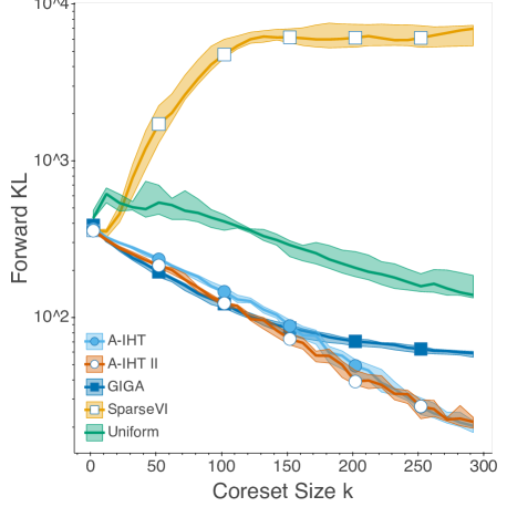
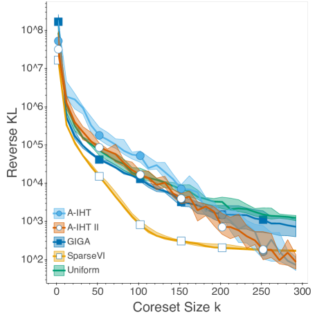
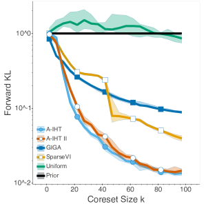
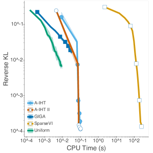
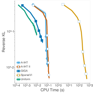
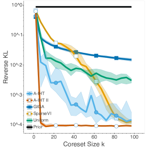
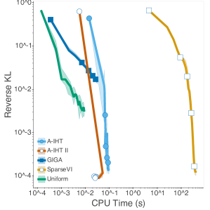
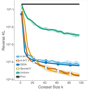
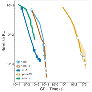
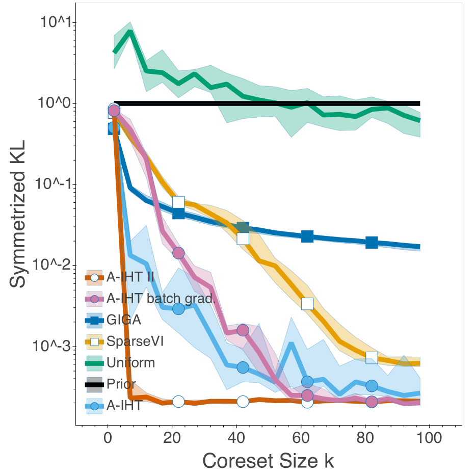
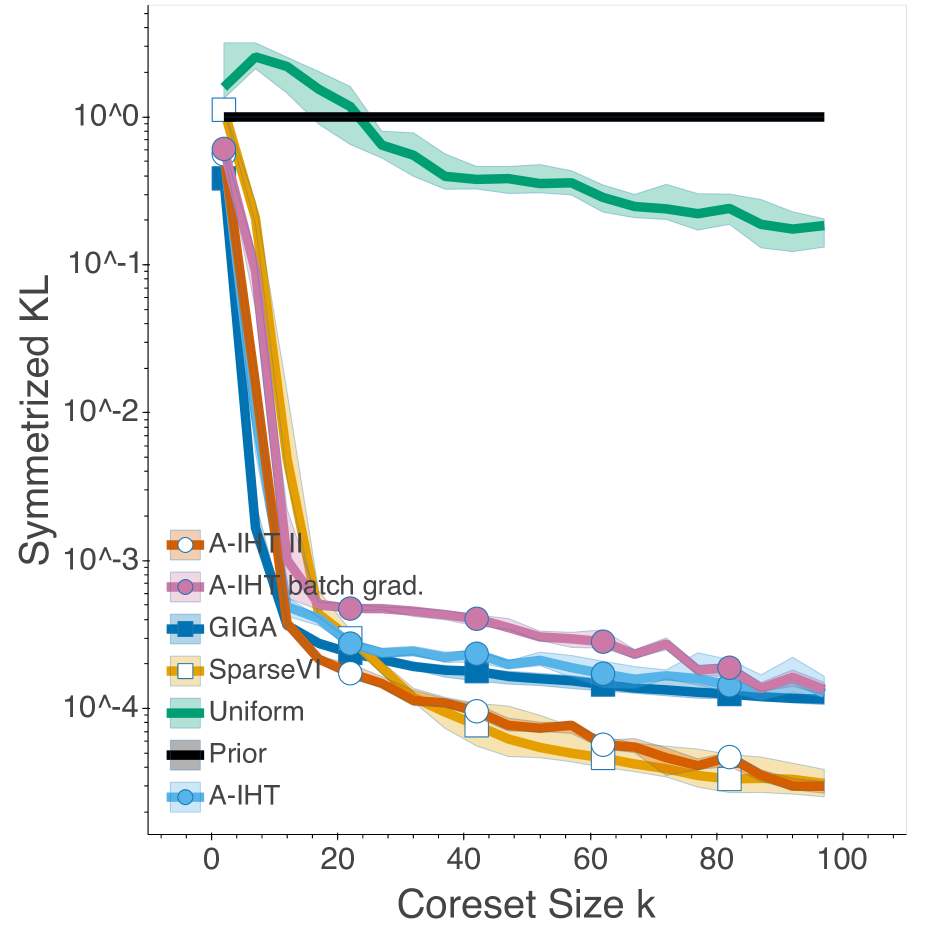
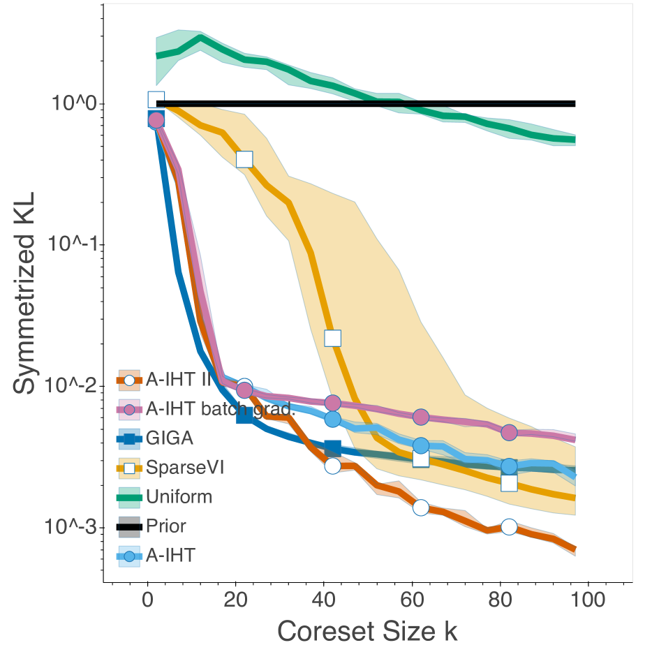
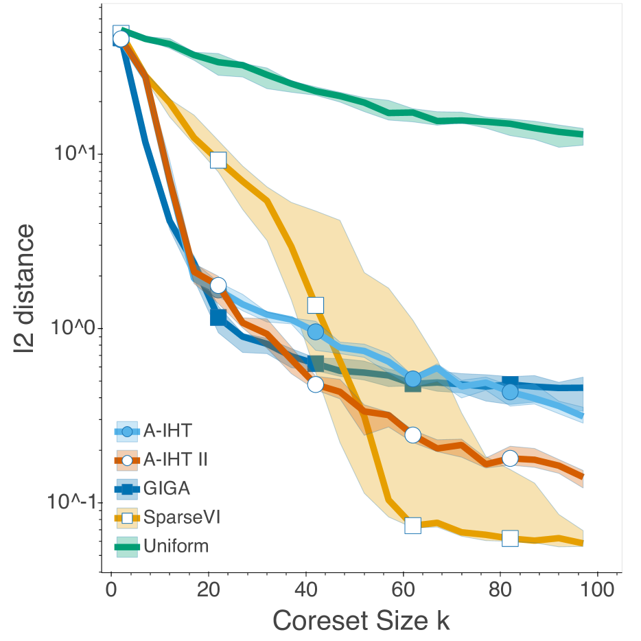
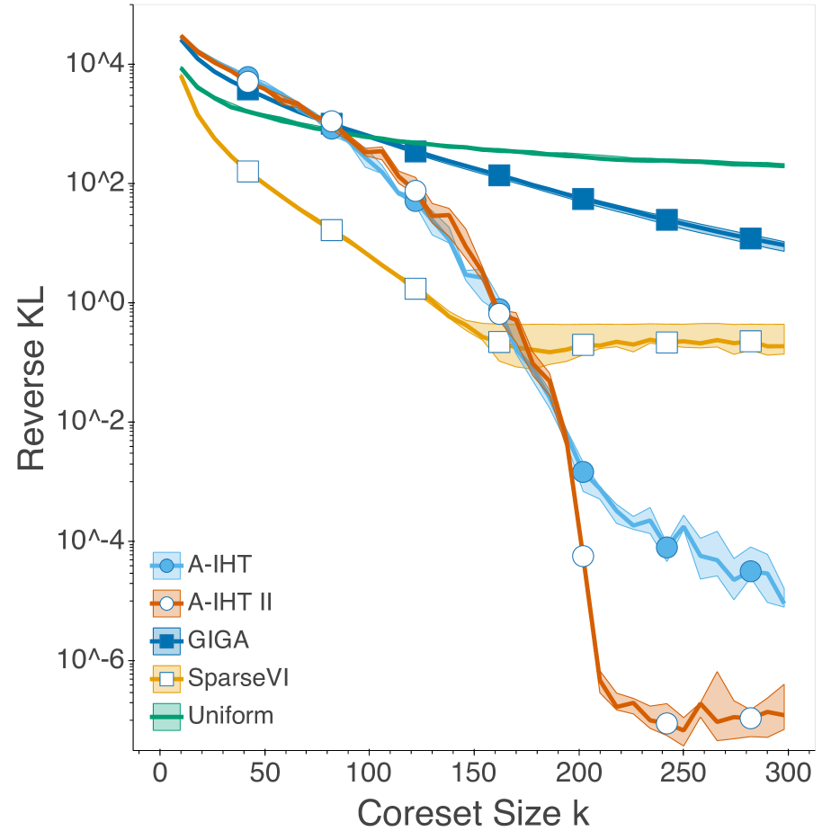
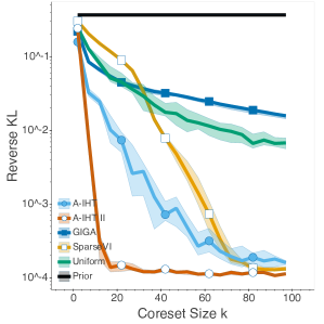
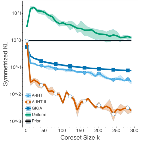
Figure 1: (a): Bayesian coresets for synthetic Gaussian posterior inference. (b): Experiments on Bayesian radial basis function regression, with the difference between true posterior and coreset posterior measured in both forward KL and reverse KL. For both (a) and (b), k𝑘k is the sparsity setting, and the solid lines are the median KL divergence between the constructed coreset posterior and true posterior over 10 trials. The shaded area is the KL divergence between 25thsuperscript25𝑡25^{th} and 75thsuperscript75𝑡75^{th} percentiles.

Other scalable approaches for Bayesian inference include subsampling and streaming methods for variational Bayes (Hoffman et al., 2013; Broderick et al., 2013), subsampling methods for MCMC (Welling & Teh, 2011; Ahn et al., 2012; Korattikara et al., 2014; Maclaurin & Adams, 2015), and consensus methods for MCMC (Srivastava et al., 2015; Rabinovich et al., 2015; Scott et al., 2016). These algorithms are motivated by empirical performance and come with few or no theoretical optimization-based guarantees on the inference quality, and often do not scale to larger datasets. Bayesian coresets could be used as part of these approaches, thus resulting into a universal tool for approximate MCMC and variational inference. Recently, Bayesian coresets have been applied to complex models and data. For example, Pinsler et al. (2019) apply Bayesian coresets to batch active learning on Bayesian neural networks with real-world image datasets.

There have been few studies that study convergence properties of approximate inference algorithms. Campbell & Beronov (2019) presented a linear convergence rate, but the assumptions they make are non-standard as the rate of convergence depends on the how well individual samples correlate with the overall loss. Approximation guarantees in terms of KL-divergence are provided (Koyejo et al., 2014; Khanna et al., 2017) for structured sparse posterior inference using the greedy forward selection procedure. Locatello et al. (2017, 2018) study convergence rates for a boosting based algorithm for iteratively refined variational inference.

Thresholding based optimization algorithms have been attractive alternatives to relaxing the constraint to a convex one or to greedy selection. Bahmani et al. (2013) provide a gradient thresholding algorithm that generalizes pursuit approaches for compressed sensing to more general losses. Yuan et al. (2018) study convergence of gradient thresholding algorithms for general losses. Jain et al. (2014) consider several variants of thresholding based algorithms for high dimensional sparse estimation. Additional related works are discussed in Section D in the appendix.

5 Experiments

We empirically examine the performance of our algorithms to construct coresets for Bayesian posterior approximation. Three sets of experiments are presented: Gaussian posterior inference, Bayesian radial basis function regression, and Bayesian logistic and Poisson regression using real-world datasets.

Besides the Automated Accelerated IHT (Algorithm 2), we propose Automated Accelerated IHT - II (Algorithm 3 in section A of appendix), that adds a de-bias step that further improves Algorithm 2 in practice. We refer to the appendix for detailed explanation and discussion of Algorithm 3 due to space limitation.

The proposed algorithms, Automated Accelerated IHT (A-IHT) and Automated Accelerated IHT II (A-IHT II), are compared with three baseline algorithms, i.e., Random (Uniform), Greedy Iterative Geodesic Ascent (GIGA) (Campbell & Broderick, 2018) and Sparse Variational Inference (SparseVI) (Campbell & Beronov, 2019). We use the public Github resources of GIGA and SparseVI for their implementation, where details are provided in our Github repository (link on page 2). We note that the Frank-Wolfe (FW) method proposed in (Campbell & Broderick, 2019) has been shown to be inferior to GIGA and SparseVI in the two corresponding articles, and thus we believe that comparing with GIGA and SparseVI is sufficient.

We calculate the Kullback–Leibler (KL) divergence between the constructed coresets posterior πwsubscript𝜋𝑤\pi_{w} and the true posterior π𝜋\pi. We measure both the forward KL divergence DKL(ππw)subscript𝐷KLconditional𝜋subscript𝜋𝑤D_{\text{KL}}(\pi\|\pi_{w}) and reverse KL divergence DKL(πwπ)subscript𝐷KLconditionalsubscript𝜋𝑤𝜋D_{\text{KL}}(\pi_{w}\|\pi). Both A-IHT and A-IHT II require minimal tuning, i.e., only the stoping criterion is required: wtwt1105wtnormsubscript𝑤𝑡subscript𝑤𝑡1superscript105normsubscript𝑤𝑡\|w_{t}-w_{t-1}\|\leq 10^{-5}\|w_{t}\|, or number of iterations >300absent300>300 for both A-IHT and A-IHT II .

5.1 Synthetic Gaussian posterior inference

We examine the algorithms in this experiment where we have closed-form exact expressions. Specifically, we compare each of these algorithms in terms of optimization accuracy without errors from sampling.
Refer to captionRefer to captionRefer to caption
Refer to captionRefer to captionRefer to captionRefer to caption
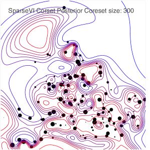
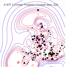
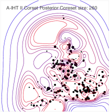
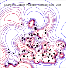
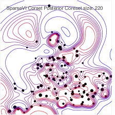
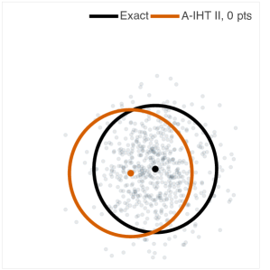
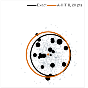
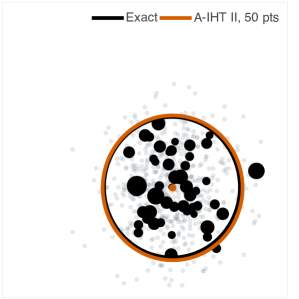
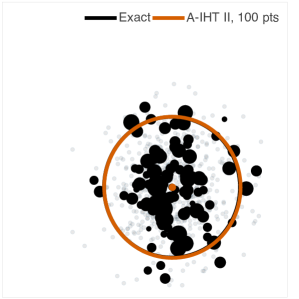
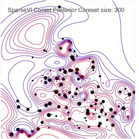
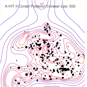
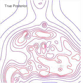
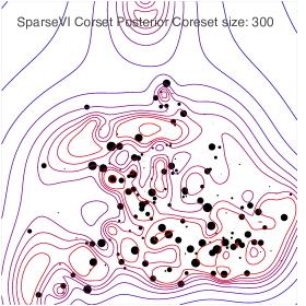
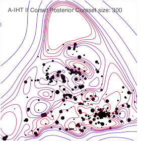
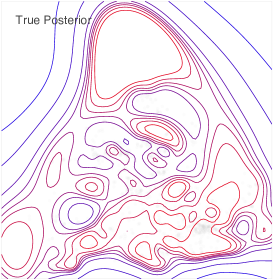
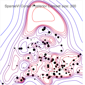
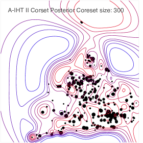
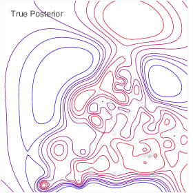
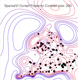
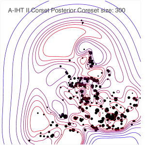
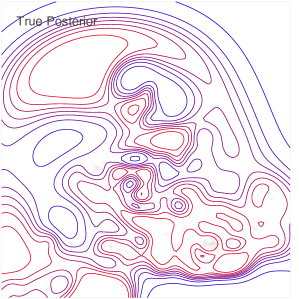
Figure 2: Experiments on Bayesian radial basis function regression, where coreset sparsity setting k=220,260,300𝑘220260300k=220,260,300. Coreset points are presented as black dots, with their radius indicating assigned weights. When k=300𝑘300k=300, posterior constructed by Accelerated IHT II (top left) shows almost exact contours as the true posterior (top middle), while posterior constructed by SparseVI (top right) shows deviated contours from the true posterior distribution.

For the D𝐷D-dimensional Gaussian distribution, we set the parameter θ𝒩(μ0,Σ0)similar-to𝜃𝒩subscript𝜇0subscriptΣ0\theta\sim\mathcal{N}(\mu_{0},\Sigma_{0}) and draw N𝑁N i.i.d. samples xn𝒩(θ,Σ)similar-tosubscript𝑥𝑛𝒩𝜃Σx_{n}{\sim}\mathcal{N}(\theta,\Sigma), which results in a Gaussian posterior distribution with closed-form parameters, as shown in  (Campbell & Beronov, 2019). We set the dimension D=200𝐷200D=200, number of samples N=600𝑁600N=600, and maximal sparsity k𝑘k is set to be 1,,30013001,\dots,300. The initial mean μ0=0subscript𝜇00\mu_{0}=0, and the initial covariance matrix is set to be Σ0=Σ=IsubscriptΣ0Σ𝐼\Sigma_{0}=\Sigma=I. The learning rate for SparseVI is γt=1/tsubscript𝛾𝑡1𝑡\gamma_{t}=1/t, and the number of weight update iterations for Sparse VI is 100100100, as suggested by their paper.

Comparison among all the 5 algorithms measuring the reverse KL divergence between the true posterior and the coreset posterior is presented in Figure 1 (a), which shows that IHT outperforms SparseVI and GIGA, achieving nearly optimal results. We observe that SparseVI stops improving once it hits certain sparsity level, which we suspect is due to the limitations of its greedy nature. It can also be observed that A-IHT II converges faster than A-IHT. Additional results are put in the section E in appendix.

5.2 Bayesian Radial Basis Function Regression

In this subsection, we explore the performance of proposed methods versus the baselines in terms of the both forward KL and reverse KL divergence. The SparseVI algorithm optimizes reverse KL; we show this does not always imply reduction in the forward KL. Indeed selecting more points to greedily optimizing the reverse KL can cause an increase in the forward KL.

Refer to captionRefer to captionRefer to caption

Top Row: synthetic dataset

Refer to captionRefer to captionRefer to caption

Bottom Row: phishing dataset

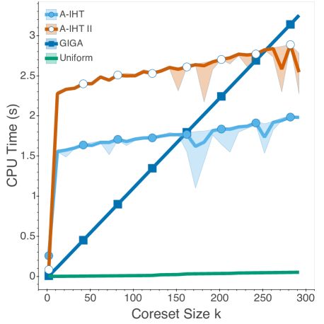
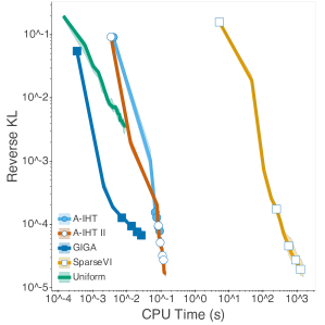
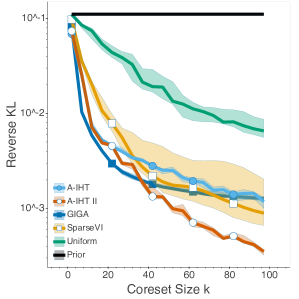
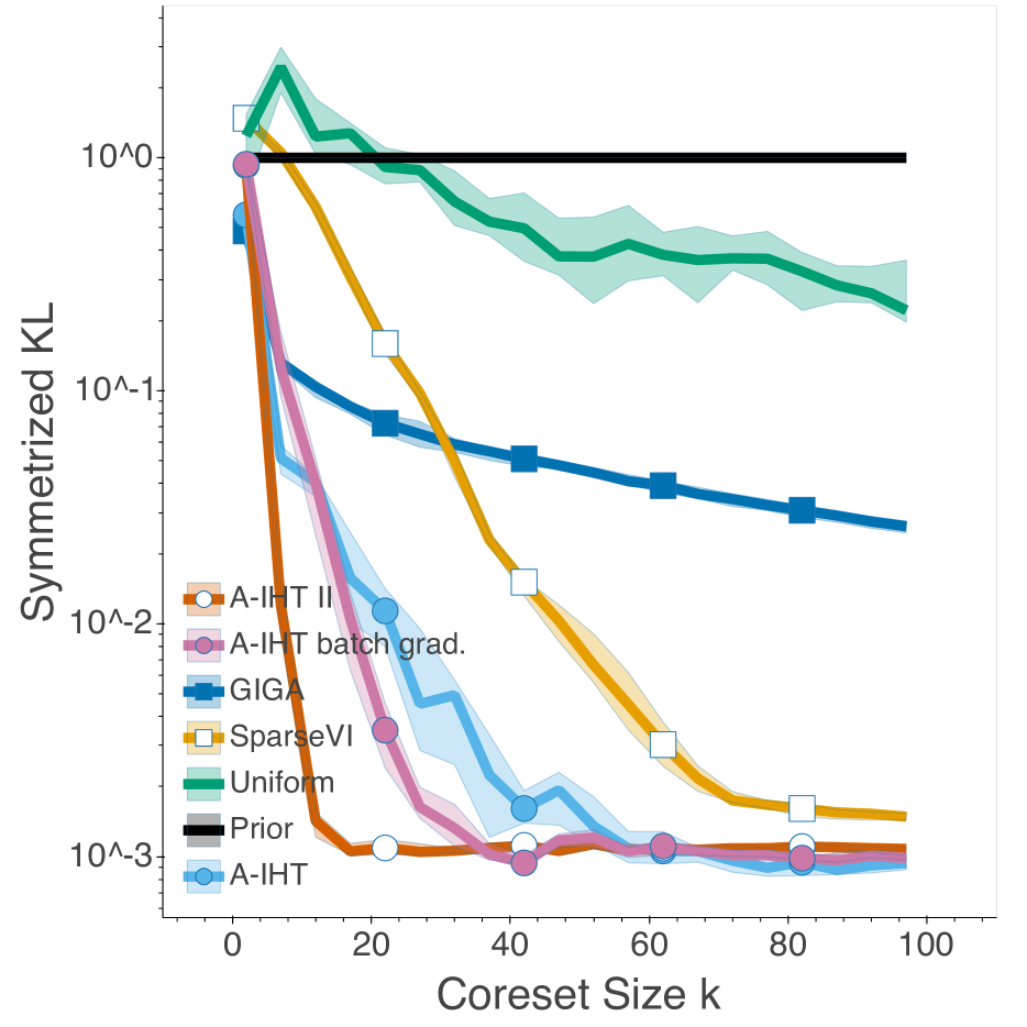
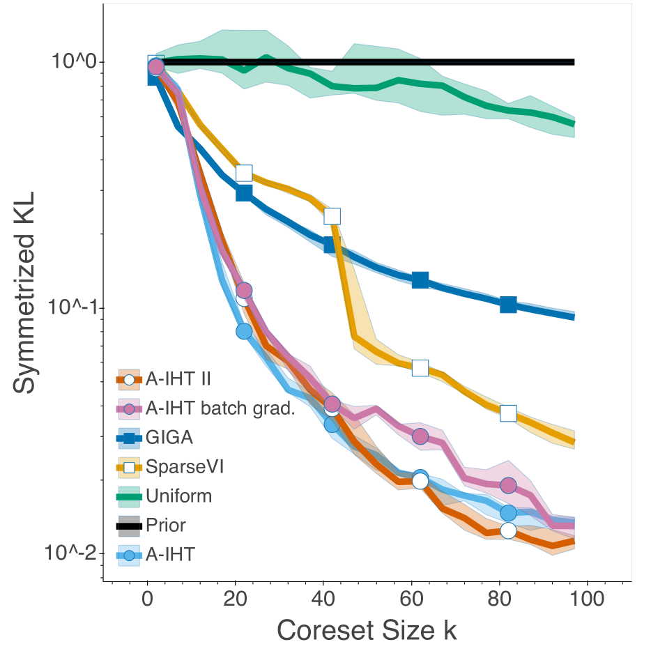
Figure 3: Bayesian coreset construction for logistic regression (LR) using the synthetic dataset (top row) and the phishing dataset (bottom row). All the algorithms are run 202020 times, and the median as well as the interval of 35thsuperscript35𝑡35^{th} and 65thsuperscript65𝑡65^{th} percentile, indicated as the shaded area, are reported. Different maximal coreset size k𝑘k is tested from 111 to 100100100. Forward KL (left column) and reverse KL (middle column) divergence between estimated true posterior and coreset posterior indicate the quality of the constructed coreset. The smaller the KL divergence, the better the coreset is. The running time for each algorithms is also recorded (right column).

We aim to infer the posterior for Bayesian radial basis function regression. Given the dataset222The task is to predict housing prices from the UK land registry data (https://www.gov.uk/government/statistical-data-sets/price-paid-data-downloads) using latitude/longitude coordinates from the Geonames postal code data (http://download.geonames.org/export/zip/) as features. {(xn,yn)2×}n=1Nsuperscriptsubscriptsubscript𝑥𝑛subscript𝑦𝑛superscript2𝑛1𝑁\{(x_{n},y_{n})\in\mathbb{R}^{2}\times\mathbb{R}\}_{n=1}^{N}, where xnsubscript𝑥𝑛x_{n} is the latitude/longitude coordinates and ynsubscript𝑦𝑛y_{n} is house-sale log-price in the United Kingdom, the goal is to infer coefficients αD𝛼superscript𝐷\alpha\in\mathbb{R}^{D} for D𝐷D radial basis functions bd(x)=exp(12σd2(xμd)2)subscript𝑏𝑑𝑥12superscriptsubscript𝜎𝑑2superscript𝑥subscript𝜇𝑑2b_{d}(x)=\exp(-\frac{1}{2\sigma_{d}^{2}}(x-\mu_{d})^{2}) for d[D]𝑑delimited-[]𝐷d\in[D]. The model is yn=bnα+ϵnsubscript𝑦𝑛superscriptsubscript𝑏𝑛top𝛼subscriptitalic-ϵ𝑛y_{n}=b_{n}^{\top}\alpha+\epsilon_{n}, where ϵn𝒩(0,σ2)similar-tosubscriptitalic-ϵ𝑛𝒩0superscript𝜎2\epsilon_{n}\sim\mathcal{N}(0,\sigma^{2}) with σ2superscript𝜎2\sigma^{2} be the variance of {yn}subscript𝑦𝑛\{y_{n}\}, and bn=[b1(xn),,bD(xn)]subscript𝑏𝑛superscriptsubscript𝑏1subscript𝑥𝑛subscript𝑏𝐷subscript𝑥𝑛topb_{n}=[b_{1}(x_{n}),\dots,b_{D}(x_{n})]^{\top}. We set prior α𝒩(μ0,σ02I)similar-to𝛼𝒩subscript𝜇0superscriptsubscript𝜎02𝐼\alpha\sim\mathcal{N}(\mu_{0},\sigma_{0}^{2}I), where μ0,σ02subscript𝜇0superscriptsubscript𝜎02\mu_{0},\sigma_{0}^{2} are empirical mean and second moment of the data. We subsampled the dataset uniformly at random to N=1000𝑁1000N=1000 records for the experiments, and generated 50 basis functions for each of the 6 scales σd{0.2,0.4,0.8,1.2,1.6,2.0}subscript𝜎𝑑0.20.40.81.21.62.0\sigma_{d}\in\{0.2,0.4,0.8,1.2,1.6,2.0\} by generating means μdsubscript𝜇𝑑\mu_{d} for each basis uniformly from data. Except for the 300300300 basis functions, an additional near-constant basis of scale 100100100, with mean corresponding to the mean latitude and longitude of the data, is added. Therefore, D=301𝐷301D=301 basis functions are considered. Each of the algorithms has access to the closed-form of posterior distribution and covariance (see (Campbell & Beronov, 2019) for detailed derivation).

Specific settings for the algorithms are as follows. For SparseVI, the exact covariance can be obtained, and the weight update step can be done without Monte Carlo estimation. For IHT and GIGA, we use true posterior for constructing the 2subscript2\ell_{2} loss function. The learning rate for SparseVI is set to be γt=1/tsubscript𝛾𝑡1𝑡\gamma_{t}=1/t, and iteration number T=100𝑇100T=100, which is the setting SparseVI uses for the experiment (Campbell & Beronov, 2019).

IHT’s objective indicates both bounded forward KL and reverse KL. However, SparseVI, which optimizes the reverse KL, offers no guarantee for the forward KL. As shown in Figure 1 (b), SparseVI increasingly deviates from the true distribution in forward KL as the coreset growths. However, IHT methods offers consistently better coresets in both the metrics.

The reverse KL divergence alone is not enough to indicate good approximation, as shown in Figure 2. We plot the posterior contours for both the true posterior and coreset posterior at a random trial when sparsity level k=220,260,300𝑘220260300k=220,260,300. The coreset posterior constructed by our Algorithm 3 recovers the true posterior almost exactly at k=300𝑘300k=300, unlike SparseVI. The results for other trials are provided in section F in the appendix.

5.3 Bayesian logistic and Poisson regression

We consider how IHT performs when used in real applications where the closed-form expressions are unattainable. Moreover, large-scale datasets are considered to test running time of each algorithm. As the true posterior is unknown, a Laplace approximation is used for GIGA and IHT to derive the finite projection of the distribution, i.e., g^isubscript^𝑔𝑖\hat{g}_{i}. Further, Monte Carlo sampling is used to derive gradients of DKLsubscript𝐷KLD_{\text{KL}} for SparseVI. We compare different algorithms estimating the posterior distribution for logistic regression and Poisson regression. The reverse KL and forward KL between the coreset posterior and true posterior are estimated using another Laplace approximation. The mode of the Laplace approximation is derived by maximizing the corresponding posterior density. The experiment was proposed by Campbell & Broderick (2019), and is used in (Campbell & Broderick, 2018) and (Campbell & Beronov, 2019). Due to space limitations, we refer to section G in the appendix for details of the experimental setup, and extensive additional results.
Refer to captionRefer to caption

Top Row: large synthetic dataset

Refer to captionRefer to caption

Bottom Row: original phishing dataset

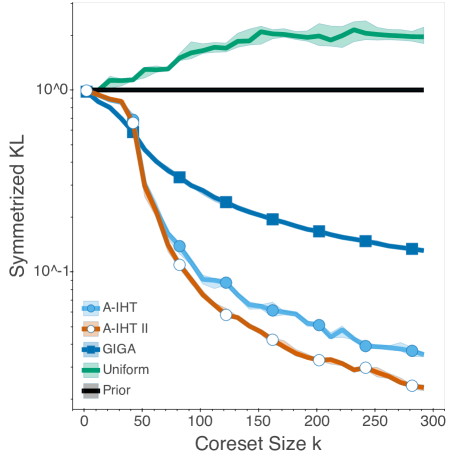
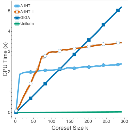
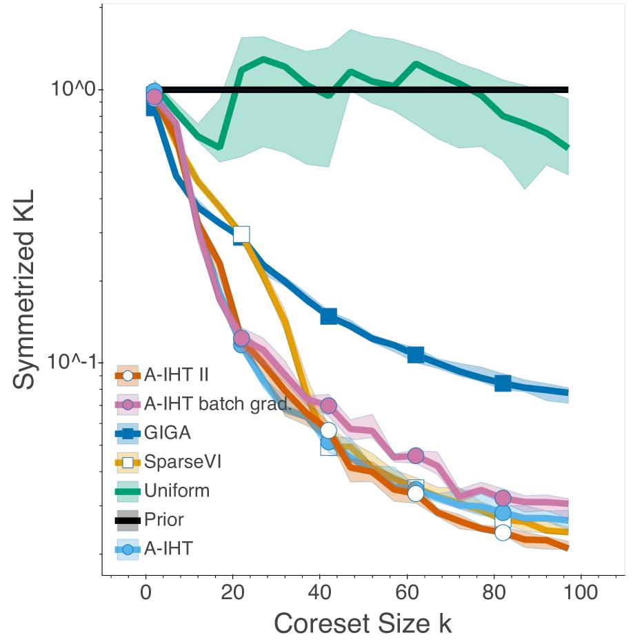
Figure 4: Bayesian coreset construction for logistic regression (LR) using the large synthetic dataset (top row) and the original phishing dataset (bottom row). All the algorithms are run 101010 times, and the median as well as the interval of 35thsuperscript35𝑡35^{th} and 65thsuperscript65𝑡65^{th} percentile, indicated as the shaded area, are reported. Different maximal coreset size k𝑘k is tested. Symmetrized KL divergence between estimated true posterior and coreset posterior indicate the quality of the constructed coreset (left column). The running time for each algorithms is also recorded (right column).

For logistic regression, given a dataset {(xn,yn)D×{1,1}n[N]}conditional-setsubscript𝑥𝑛subscript𝑦𝑛superscript𝐷11𝑛delimited-[]𝑁\{(x_{n},y_{n})\in\mathbb{R}^{D}\times\{1,-1\}\mid n\in[N]\}, we aim to infer θD+1𝜃superscript𝐷1\theta\in\mathbb{R}^{D+1} based on the model:

ynxn,θBern(11+eznθ),similar-toconditionalsubscript𝑦𝑛subscript𝑥𝑛𝜃Bern11superscript𝑒superscriptsubscript𝑧𝑛top𝜃\displaystyle y_{n}\mid x_{n},\theta\sim\text{Bern}\left(\frac{1}{1+e^{-z_{n}^{\top}\theta}}\right), (11)

where zn=[xn,1]subscript𝑧𝑛superscriptsuperscriptsubscript𝑥𝑛top1topz_{n}=[x_{n}^{\top},1]^{\top}. We set N=500𝑁500N=500 by uniformly sub-sampling from datasets due to the high computation cost of SparseVI. Three datasets are used for logistic regression. Two of them are: the synthetic dataset consists of xnsubscript𝑥𝑛x_{n} sampled i.i.d. from normal distribution 𝒩(0,I)𝒩0𝐼{\mathcal{N}}(0,I), and label ynsubscript𝑦𝑛y_{n} sampled from Bernoulli distribution conditioned on xnsubscript𝑥𝑛x_{n} and θ=[3,3,0]𝜃superscript330top\theta=[3,3,0]^{\top}. The phishing dataset333https://www.csie.ntu.edu.tw/~cjlin/libsvmtools/datasets/binary.html is preprocessed (Campbell & Beronov, 2019) via PCA to dimension of D=10𝐷10D=10 to mitigate high computation by SparseVI.

We present two sets of experiments, i.e., logistic regression using the synthetic dataset and the phishing dataset, in Figure 3. One other set of experiments on logistic regression, and three sets of experiments on Poisson regression are deferred to section G in appendix.

It is observed that A-IHT and A-IHT II achieve state-of-the-art performance. The IHT algorithms often obtain coresets with smaller KL between the coreset posterior and true posterior than GIGA and SparseVI, with computing time comparable to GIGA and significantly less than SparseVI. We conjecture that GIGA and SparseVI perform worse than our methods due to their greedy nature: they can be "short-sighted" and do not rectify past decisions. The experiments indicate that IHT outperforms the previous methods, improving the trade-off between accuracy and performance.

Large-scale Datasets. Two large datasets are considered: i)i) the large synthetic dataset for logistic regression is generated following the same procedure as before, but with dataset size N=9000𝑁9000N=9000; ii)ii) the original phishing dataset has size N=11055𝑁11055N=11055 and dimension D=68𝐷68D=68. The maximal iteration number of the two IHT algorithms is 500500500. Symmetrized KL, i.e., the sum of forward and reverse KL, is reported.

Results are shown in Figure 4. We have to omit SparseVI due to its prohibitively high cost (e.g., as shown in Figure 3, SparseVI needs ×104absentsuperscript104\times 10^{4} more time than IHT and GIGA). As our complexity analysis of the algorithms in subsection 3.2, the running time of GIGA grows linearly with respect to the coreset size k𝑘k, while that is almost free for IHT. GIGA begins to cost more time than IHT at k200𝑘200k\approx 200, i.e., about only 2%percent22\% of the dataset.

Additional evaluation. For large-scale datasets, it is often necessary to "batch" the algorithms. We test the performance of IHT using a stochastic gradient estimator. The gradient estimator is calculated with random batches in each iteration, where we use a batch size of 20%percent2020\% of the full dataset size. Results on six datasets are defer to section G in appendix.

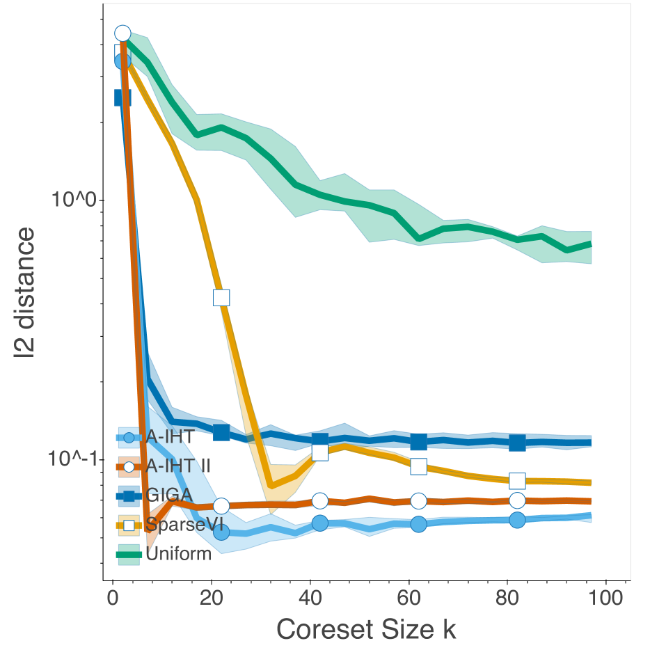
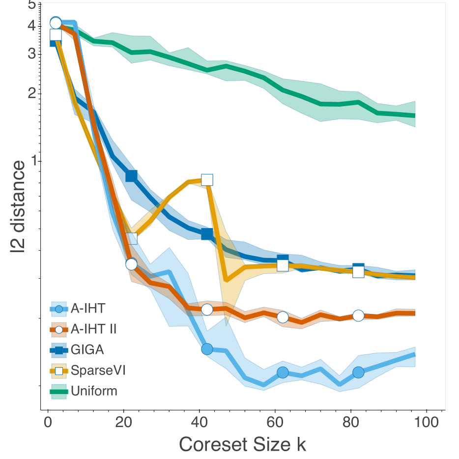
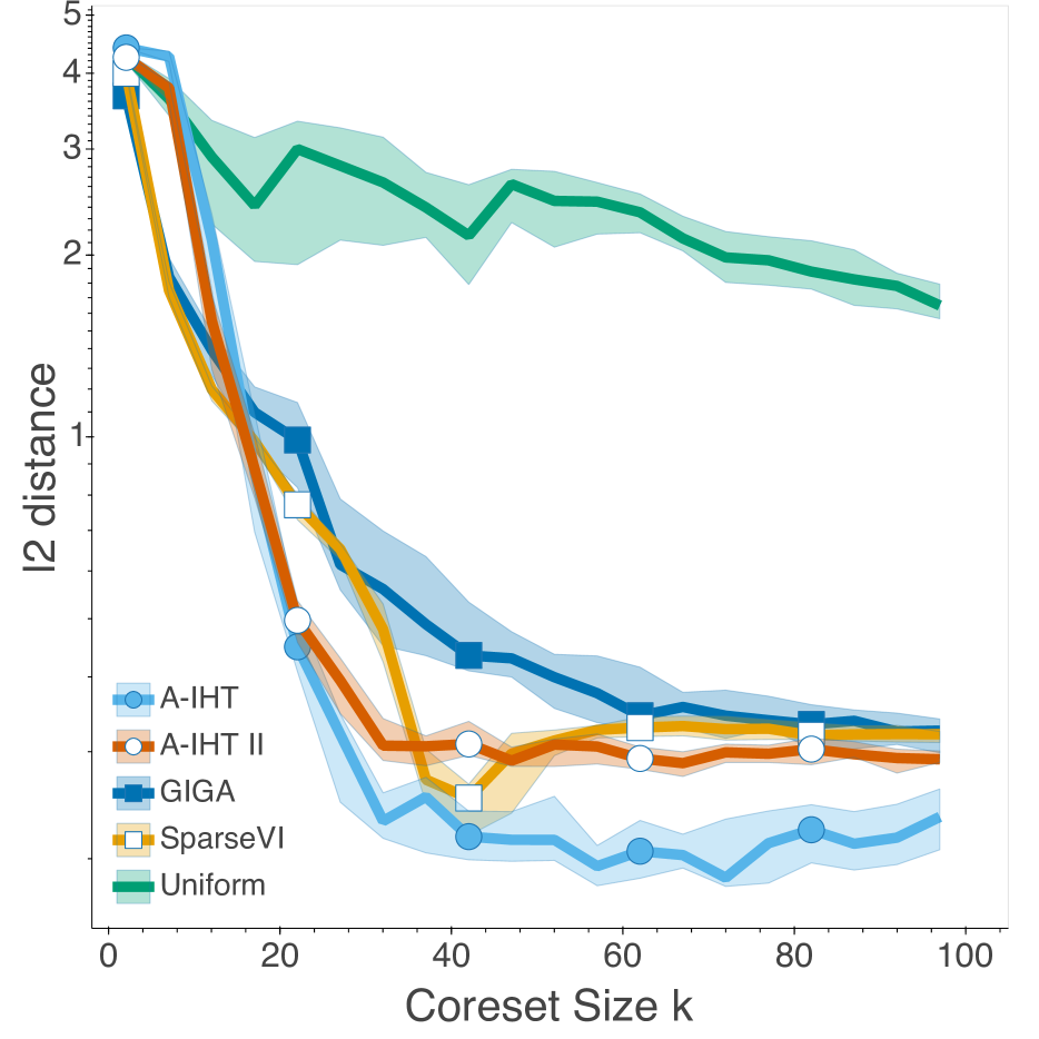
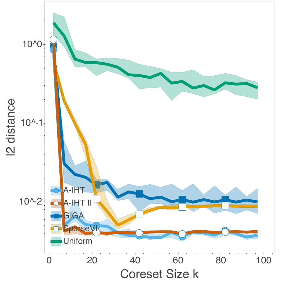
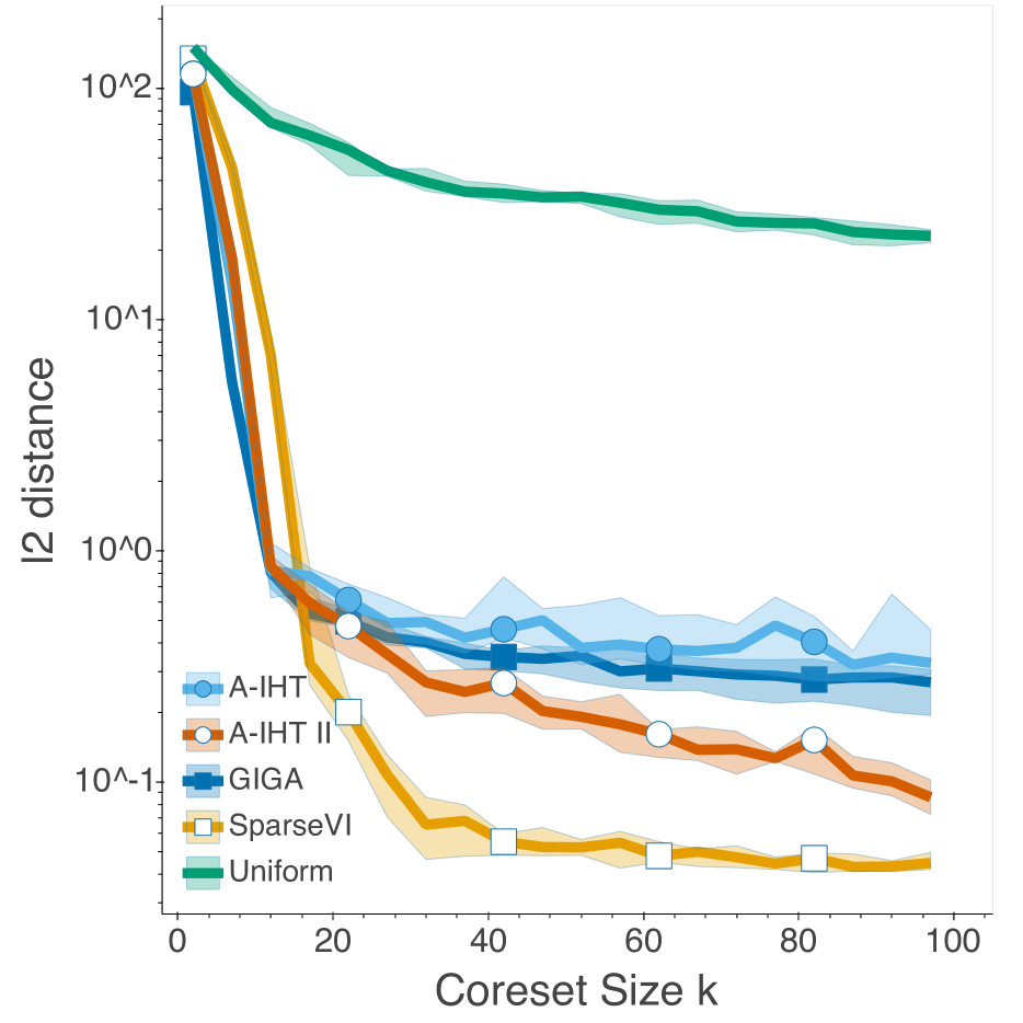
Moreover, as an alternative evaluation of the quality of constructed coresets, we test the 2subscript2\ell_{2}-distance between the maximum-a-posteriori (MAP) estimation of the full-dataset posterior and coreset posterior. Results on six datasets are deferred to section G in appendix.

6 Conclusion

In this paper, we consider the Bayesian coreset construction problem from a sparse optimization perspective, through which we propose a new algorithm that incorporates the paradigms of sparse as well as accelerated optimization. We provide theoretical analysis for our method, showing linear convergence under standard assumptions. Finally, numerical results demonstrate the improvement in both accuracy and efficiency when compared to the state of the art methods. Our viewpoint of using sparse optimization for Bayesian coresets can potentially help to consider more complex structured sparsity, which is left as future work.

Acknowledgements

AK acknowledges funding by the NSF (CCF-1907936, CNS-2003137). AK thanks TOOL’s Danny Carey for his percussion performance in “Pneuma”. We would like to thank the reviewers for their valuable and constructive comments. Their feedback enables us to further improve the paper.

References

  • Ahn et al. (2012) Sungjin Ahn, Anoop Korattikara, and Max Welling. Bayesian posterior sampling via stochastic gradient fisher scoring. In 29th International Conference on Machine Learning, ICML 2012, pp.  1591–1598, 2012.
  • Bahmani et al. (2013) Sohail Bahmani, Bhiksha Raj, and Petros T. Boufounos. Greedy sparsity-constrained optimization. J. Mach. Learn. Res., 14(1):807–841, March 2013. ISSN 1532-4435.
  • Baldassarre et al. (2016) Luca Baldassarre, Nirav Bhan, Volkan Cevher, Anastasios Kyrillidis, and Siddhartha Satpathi. Group-sparse model selection: Hardness and relaxations. IEEE Transactions on Information Theory, 62(11):6508–6534, 2016.
  • Baraniuk et al. (2008) Richard Baraniuk, Mark A. Davenport, Ronald A. DeVore, and Michael B. Wakin. A simple proof of the restricted isometry property for random matrices. Constructive Approximation, 28:253–263, 2008.
  • Baraniuk et al. (2010) Richard G Baraniuk, Volkan Cevher, Marco F Duarte, and Chinmay Hegde. Model-based compressive sensing. IEEE Transactions on information theory, 56(4):1982–2001, 2010.
  • Beck & Teboulle (2009) Amir Beck and Marc Teboulle. A fast iterative shrinkage-thresholding algorithm for linear inverse problems. SIAM J. Imaging Sciences, 2:183–202, 2009.
  • Blumensath & Davies (2009) T. Blumensath and M. Davies. Iterative hard thresholding for compressed sensing. Applied and computational harmonic analysis, 27(3):265–274, 2009.
  • Blumensath (2012) Thomas Blumensath. Accelerated iterative hard thresholding. Signal Process., 92(3):752–756, March 2012. ISSN 0165-1684. doi: 10.1016/j.sigpro.2011.09.017. URL https://doi.org/10.1016/j.sigpro.2011.09.017.
  • Blumensath & Davies (2010) Thomas Blumensath and Mike E Davies. Normalized iterative hard thresholding: Guaranteed stability and performance. IEEE Journal of selected topics in signal processing, 4(2):298–309, 2010.
  • Broderick et al. (2013) Tamara Broderick, Nicholas Boyd, Andre Wibisono, Ashia C Wilson, and Michael I Jordan. Streaming variational bayes. In Advances in Neural Information Processing Systems, pp. 1727–1735, 2013.
  • Campbell & Beronov (2019) Trevor Campbell and Boyan Beronov. Sparse variational inference: Bayesian coresets from scratch. In Advances in Neural Information Processing Systems, pp. 11457–11468, 2019.
  • Campbell & Broderick (2018) Trevor Campbell and Tamara Broderick. Bayesian coreset construction via greedy iterative geodesic ascent. In International Conference on Machine Learning, pp. 697–705, 2018.
  • Campbell & Broderick (2019) Trevor Campbell and Tamara Broderick. Automated scalable bayesian inference via hilbert coresets. The Journal of Machine Learning Research, 20(1):551–588, 2019.
  • Candes (2008) Emmanuel J Candes. The restricted isometry property and its implications for compressed sensing. Comptes rendus mathematique, 346(9-10):589–592, 2008.
  • Chen & Sanghavi (2010) Yuxin Chen and Sujay Sanghavi. A general framework for high-dimensional estimation in the presence of incoherence. In 2010 48th Annual Allerton Conference on Communication, Control, and Computing (Allerton), pp.  1570–1576. IEEE, 2010.
  • Dai & Milenkovic (2009) Wei Dai and Olgica Milenkovic. Subspace pursuit for compressive sensing signal reconstruction. IEEE transactions on Information Theory, 55(5):2230–2249, 2009.
  • Donoho et al. (2006) David L Donoho et al. Compressed sensing. IEEE Transactions on information theory, 52(4):1289–1306, 2006.
  • Foucart (2011) Simon Foucart. Hard thresholding pursuit: an algorithm for compressive sensing. SIAM Journal on Numerical Analysis, 49(6):2543–2563, 2011.
  • Frank & Wolfe (1956) Marguerite Frank and Philip Wolfe. An algorithm for quadratic programming. Naval research logistics quarterly, 3(1-2):95–110, 1956.
  • Ghadimi et al. (2015) E. Ghadimi, H. R. Feyzmahdavian, and M. Johansson. Global convergence of the heavy-ball method for convex optimization. In 2015 European Control Conference (ECC), pp.  310–315, July 2015.
  • Hoffman et al. (2013) Matthew D Hoffman, David M Blei, Chong Wang, and John Paisley. Stochastic variational inference. The Journal of Machine Learning Research, 14(1):1303–1347, 2013.
  • Huggins et al. (2016) Jonathan Huggins, Trevor Campbell, and Tamara Broderick. Coresets for scalable bayesian logistic regression. In Advances in Neural Information Processing Systems, pp. 4080–4088, 2016.
  • Jaggi (2013) Martin Jaggi. Revisiting frank-wolfe: Projection-free sparse convex optimization. In Proceedings of the 30th international conference on machine learning, pp.  427–435, 2013.
  • Jain et al. (2014) Prateek Jain, Ambuj Tewari, and Purushottam Kar. On iterative hard thresholding methods for high-dimensional m-estimation. In Proceedings of the 27th International Conference on Neural Information Processing Systems - Volume 1, NIPS’14, pp.  685–693, Cambridge, MA, USA, 2014. MIT Press.
  • Jain et al. (2016) Prateek Jain, Nikhil Rao, and Inderjit S Dhillon. Structured sparse regression via greedy hard thresholding. In Advances in Neural Information Processing Systems, pp. 1516–1524, 2016.
  • Khanna & Kyrillidis (2018) Rajiv Khanna and Anastasios Kyrillidis. Iht dies hard: Provable accelerated iterative hard thresholding. In International Conference on Artificial Intelligence and Statistics, pp.  188–198, 2018.
  • Khanna et al. (2017) Rajiv Khanna, Joydeep Ghosh, Rusell Poldrack, and Oluwasanmi Koyejo. Information projection and approximate inference for structured sparse variables. In Artificial Intelligence and Statistics, pp.  1358–1366, 2017.
  • Korattikara et al. (2014) Anoop Korattikara, Yutian Chen, and Max Welling. Austerity in mcmc land: Cutting the metropolis-hastings budget. In International Conference on Machine Learning, pp. 181–189, 2014.
  • Koyejo et al. (2014) Oluwasanmi Koyejo, Rajiv Khanna, Joydeep Ghosh, and Russell A. Poldrack. On prior distributions and approximate inference for structured variables. In Proceedings of the 27th International Conference on Neural Information Processing Systems - Volume 1, NIPS’14, pp.  676–684, Cambridge, MA, USA, 2014. MIT Press.
  • Kyrillidis & Cevher (2011) Anastasios Kyrillidis and Volkan Cevher. Recipes on hard thresholding methods. In 2011 4th IEEE International Workshop on Computational Advances in Multi-Sensor Adaptive Processing (CAMSAP), pp.  353–356. IEEE, 2011.
  • Kyrillidis & Cevher (2014) Anastasios Kyrillidis and Volkan Cevher. Matrix recipes for hard thresholding methods. Journal of Mathematical Imaging and Vision, 2(48):235–265, 2014.
  • Kyrillidis et al. (2015) Anastasios Kyrillidis, Luca Baldassarre, Marwa El Halabi, Quoc Tran-Dinh, and Volkan Cevher. Structured sparsity: Discrete and convex approaches. In Compressed Sensing and its Applications, pp.  341–387. Springer, 2015.
  • Li et al. (2016) Xingguo Li, Tuo Zhao, Raman Arora, Han Liu, and Jarvis Haupt. Stochastic variance reduced optimization for nonconvex sparse learning. In Maria Florina Balcan and Kilian Q. Weinberger (eds.), Proceedings of The 33rd International Conference on Machine Learning, volume 48 of Proceedings of Machine Learning Research, pp.  917–925, New York, New York, USA, 20–22 Jun 2016. PMLR.
  • Locatello et al. (2017) Francesco Locatello, Rajiv Khanna, Joydeep Ghosh, and Gunnar Rätsch. Boosting variational inference: an optimization perspective. In AISTATS, 2017.
  • Locatello et al. (2018) Francesco Locatello, Gideon Dresdner, Rajiv Khanna, Isabel Valera, and Gunnar Rätsch. Boosting black box variational inference. In Proceedings of the 32nd International Conference on Neural Information Processing Systems, NIPS’18, pp.  3405–3415, Red Hook, NY, USA, 2018. Curran Associates Inc.
  • Ma et al. (2019) Yi-An Ma, Yuansi Chen, Chi Jin, Nicolas Flammarion, and Michael I. Jordan. Sampling can be faster than optimization. Proceedings of the National Academy of Sciences, 116(42):20881–20885, 2019. ISSN 0027-8424. doi: 10.1073/pnas.1820003116.
  • Maclaurin & Adams (2015) Dougal Maclaurin and Ryan Prescott Adams. Firefly monte carlo: Exact mcmc with subsets of data. In Twenty-Fourth International Joint Conference on Artificial Intelligence, 2015.
  • Needell & Tropp (2009) Deanna Needell and Joel A Tropp. Cosamp: Iterative signal recovery from incomplete and inaccurate samples. Applied and computational harmonic analysis, 26(3):301–321, 2009.
  • Nesterov (1983) Yurii E Nesterov. A method for solving the convex programming problem with convergence rate o(1/k2)𝑜1superscript𝑘2o(1/k^{2}). In Dokl. akad. nauk Sssr, volume 269, pp.  543–547, 1983.
  • Nguyen et al. (2014) Nam Nguyen, Deanna Needell, and Tina Woolf. Linear convergence of stochastic iterative greedy algorithms with sparse constraints. IEEE Transactions on Information Theory, 63:6869–6895, 2014.
  • Pinsler et al. (2019) Robert Pinsler, Jonathan Gordon, Eric Nalisnick, and José Miguel Hernández-Lobato. Bayesian batch active learning as sparse subset approximation. Advances in Neural Information Processing Systems, 32:6359–6370, 2019.
  • Rabinovich et al. (2015) Maxim Rabinovich, Elaine Angelino, and Michael I Jordan. Variational consensus monte carlo. In Advances in Neural Information Processing Systems, pp. 1207–1215, 2015.
  • Scott et al. (2016) Steven L Scott, Alexander W Blocker, Fernando V Bonassi, Hugh A Chipman, Edward I George, and Robert E McCulloch. Bayes and big data: The consensus monte carlo algorithm. International Journal of Management Science and Engineering Management, 11(2):78–88, 2016.
  • Shalev-Shwartz et al. (2010) Shai Shalev-Shwartz, Nathan Srebro, and Tong Zhang. Trading accuracy for sparsity in optimization problems with sparsity constraints. SIAM J. on Optimization, 20(6):2807–2832, August 2010. ISSN 1052-6234. doi: 10.1137/090759574.
  • Srivastava et al. (2015) Sanvesh Srivastava, Volkan Cevher, Quoc Dinh, and David Dunson. Wasp: Scalable bayes via barycenters of subset posteriors. In Artificial Intelligence and Statistics, pp.  912–920, 2015.
  • Tropp & Gilbert (2007) Joel A Tropp and Anna C Gilbert. Signal recovery from random measurements via orthogonal matching pursuit. IEEE Transactions on information theory, 53(12):4655–4666, 2007.
  • Welling & Teh (2011) Max Welling and Yee W Teh. Bayesian learning via stochastic gradient langevin dynamics. In Proceedings of the 28th international conference on machine learning (ICML-11), pp.  681–688, 2011.
  • Yuan et al. (2018) Xiao-Tong Yuan, Ping Li, and Tong Zhang. Gradient hard thresholding pursuit. Journal of Machine Learning Research, 18(166):1–43, 2018.
  • Zhang et al. (2019) Jacky Y Zhang, Rajiv Khanna, Anastasios Kyrillidis, and Oluwasanmi O Koyejo. Learning sparse distributions using iterative hard thresholding. In Advances in Neural Information Processing Systems 32, pp. 6757–6766. Curran Associates, Inc., 2019.

Bayesian Coresets:
Revisiting the Nonconvex Optimization Perspective
Appendix

Appendix Contents

  • Section A: Automated Accelerated IHT with de-bias step (Algorithm 3).

  • Section B: Theoretical Analysis

    • Detailed theoretical analysis on the convergence of our main algorithm, i.e., Automated Accelerated IHT in Algorithm 2.

  • Section C: Proofs

    • Proofs of the theories presented in section B.

  • Section D: Additional related work.

  • Section E: Additional Results for Synthetic Gaussian Posterior Inference (experiments introduced in section 5.1).

    • Convergence speed of the two proposed IHT algorithms.

    • Illustration of the coresets constructed by A-IHT II.

  • Section F: Additional Results for Radial Basis Regression (experiments introduced in section 5.2).

    • Additional experimental results of posterior contours for the radial basis regression experiment.

  • Section G: Details and Extensive Results of the Bayesian logistic and Poisson regression Experiments (experiments introduced in section 5.3).

    • Details of the Bayesian logistic and Poisson regression Experiments.

    • Results on all of the six datasets.

    • Results with a stochastic gradient estimator using batches of data.

    • Results with alternative evaluation on coresets quality—2subscript2\ell_{2}-distance between the maximum-a-posteriori (MAP) estimation of the full-dataset posterior and coreset posterior.

Appendix A Automated Accelerated IHT with De-bias Step

In the main text, we mention that Algorithm 2 can be boosted better in practice using de-bias steps. Here we present the algorithm with de-bias step, as shown in Algorithm 3.

Like Automated Accelerated IHT, Algorithm 3 also starts with active subspace expansion, i.e., line 3 & 4. As 𝒵=supp(zt)=supp(wt1)supp(wt)𝒵suppsubscript𝑧𝑡suppsubscript𝑤𝑡1suppsubscript𝑤𝑡{\mathcal{Z}}=\text{supp}(z_{t})=\text{supp}(w_{t-1})\cup\text{supp}(w_{t}) is a 2k2𝑘2k-sparse index set, the expanded index set 𝒮𝒮{\mathcal{S}} is a 3k3𝑘3k-sparse index set that is the union of the support of three elements, i.e.,

𝒮=supp(wt1)supp(wt)supp(Π𝒞k\𝒵(f(zt))).𝒮suppsubscript𝑤𝑡1suppsubscript𝑤𝑡suppsubscriptΠ\subscript𝒞𝑘𝒵𝑓subscript𝑧𝑡\displaystyle{\mathcal{S}}=\text{supp}(w_{t-1})\cup\text{supp}(w_{t})\cup\text{supp}(\Pi_{\mathcal{C}_{k}\backslash{\mathcal{Z}}}\left(\nabla f(z_{t})\right)). (12)

We note that, with a little abuse of notation, we use 𝒵𝒵{\mathcal{Z}} to denote both the support set 𝒵[n]𝒵delimited-[]𝑛\mathcal{Z}\subset[n], and the subspace restricted by the support, i.e., {xnsupp(x)𝒵}conditional-set𝑥superscript𝑛supp𝑥𝒵\{x\in{\mathbb{R}}^{n}\mid\text{supp}(x)\subseteq\mathcal{Z}\}, depending on the context.

The subspace corresponding to this index set 𝒮𝒮{\mathcal{S}} is a subspace that the algorithm considers as potential to achieve low loss within. Therefore, in the next step, we perform projected gradient descent in this expanded subspace. Note that we use f()|𝒮evaluated-at𝑓𝒮\nabla f(\cdot)\big{|}_{{\mathcal{S}}} to denote a sparse subset 𝒮𝒮{\mathcal{S}} of the gradient, i.e., setting the ithsuperscript𝑖𝑡i^{th} entry of f()𝑓\nabla f(\cdot) to 00 if i𝒮𝑖𝒮i\notin{\mathcal{S}}.

The projected gradient descent step consists of three sub-steps, i.e., step size selection (line 6), gradient descent (line 7), and projection to non-negative k𝑘k-sparse restricted domain (line 7). The step size selection is performed by an exact line search to obtain a good step size automatically. The projection step (line 7) is where we do “hard thresholding” to obtain a k𝑘k-sparse solution xtsubscript𝑥𝑡x_{t}. As mentioned before, this projection step can be done optimally in the sense of 2subscript2\ell_{2}-norm by choosing the k𝑘k-largest non-negative elements.

Then, we come to the key difference between Algorithm 2 and Algorithm 3, i.e., the de-bias step at line 8, 9 & 10. With additional de-bias steps, we adjust the solution k𝑘k-sparse solution xtsubscript𝑥𝑡x_{t} inside its own sparse space, i.e., the space corresponding to supp(xt)suppsubscript𝑥𝑡\text{supp}(x_{t}), such that a better k𝑘k-sparse solution is found. After computing the gradient (line 8), another exact line search is performed (line 9). By gradient descent and imposing the non-negativity constraint (line 10), we have the solution wt+1subscript𝑤𝑡1w_{t+1} for this iteration.

Lastly, the momentum step (line 11 & 12) is the same as Algorithm 2. We select the momentum term as the minimizer of the objective: τt+1=argminτf(wt+1+τ(wt+1wt))subscript𝜏𝑡1subscriptargmin𝜏𝑓subscript𝑤𝑡1𝜏subscript𝑤𝑡1subscript𝑤𝑡\tau_{t+1}=\operatorname*{arg\,min}_{\tau}f(w_{t+1}+\tau(w_{t+1}-w_{t})), and then apply the momentum to our solutions wt+1subscript𝑤𝑡1w_{t+1} and wtsubscript𝑤𝑡w_{t} as zt+1=wt+1+τt+1(wt+1wt)subscript𝑧𝑡1subscript𝑤𝑡1subscript𝜏𝑡1subscript𝑤𝑡1subscript𝑤𝑡z_{t+1}=w_{t+1}+\tau_{t+1}(w_{t+1}-w_{t}) to capture memory in the algorithm. Momentum can offer faster convergence rate for convex optimization (Nesterov, 1983).

Algorithm 3 Automated Accelerated IHT - II (A-IHT II)
0:  Objective f(w)=yΦw22𝑓𝑤superscriptsubscriptnorm𝑦Φ𝑤22f(w)=\|y-\Phi w\|_{2}^{2}; sparsity k𝑘k
1:  t=0𝑡0t=0, z0=0subscript𝑧00z_{0}=0, w0=0subscript𝑤00w_{0}=0
2:  repeat
3:     𝒵=supp(zt)𝒵suppsubscript𝑧𝑡{\mathcal{Z}}=\text{supp}(z_{t})
4:     𝒮=supp(Π𝒞k\𝒵(f(zt)))𝒵𝒮suppsubscriptΠ\subscript𝒞𝑘𝒵𝑓subscript𝑧𝑡𝒵\mathcal{S}=\text{supp}(\Pi_{\mathcal{C}_{k}\backslash{\mathcal{Z}}}\left(\nabla f(z_{t})\right))\cup{\mathcal{Z}} where |𝒮|3k𝒮3𝑘|{\mathcal{S}}|\leq 3k {active subspace expansion}
5:     ~(1)=f(zt)|𝒮superscript~1evaluated-at𝑓subscript𝑧𝑡𝒮\widetilde{\nabla}^{(1)}=\nabla f(z_{t})\big{|}_{\mathcal{S}}
6:     μt(1)=argminμf(ztμ~(1))=~(1)222Φ~(1)22superscriptsubscript𝜇𝑡1subscriptargmin𝜇𝑓subscript𝑧𝑡𝜇superscript~1superscriptsubscriptnormsuperscript~1222subscriptsuperscriptnormΦsuperscript~122\mu_{t}^{(1)}=\operatorname*{arg\,min}_{\mu}f(z_{t}-\mu\widetilde{\nabla}^{(1)})=\frac{\|\widetilde{\nabla}^{(1)}\|_{2}^{2}}{2\|\Phi\widetilde{\nabla}^{(1)}\|^{2}_{2}} {step size selection}
7:     xt=Π𝒞k+n(ztμt(1)f(zt))subscript𝑥𝑡subscriptΠsubscript𝒞𝑘subscriptsuperscript𝑛subscript𝑧𝑡superscriptsubscript𝜇𝑡1𝑓subscript𝑧𝑡x_{t}=\Pi_{\mathcal{C}_{k}\cap{\mathbb{R}}^{n}_{+}}\left(z_{t}-\mu_{t}^{(1)}{\nabla}f(z_{t})\right) {projected gradient descent}
8:     ~(2)=f(xt)|supp(x)superscript~2evaluated-at𝑓subscript𝑥𝑡supp𝑥\widetilde{\nabla}^{(2)}=\nabla f(x_{t})\big{|}_{\text{supp}(x)}
9:     μt(2)=argminμf(xtμ~(2))=~(2)222Φ~(2)22superscriptsubscript𝜇𝑡2subscriptargmin𝜇𝑓subscript𝑥𝑡𝜇superscript~2superscriptsubscriptnormsuperscript~2222subscriptsuperscriptnormΦsuperscript~222\mu_{t}^{(2)}=\operatorname*{arg\,min}_{\mu}f(x_{t}-\mu\widetilde{\nabla}^{(2)})=\frac{\|\widetilde{\nabla}^{(2)}\|_{2}^{2}}{2\|\Phi\widetilde{\nabla}^{(2)}\|^{2}_{2}} {step size selection}
10:     wt+1=Π+n(xtμt(2)~(2))subscript𝑤𝑡1subscriptΠsubscriptsuperscript𝑛subscript𝑥𝑡superscriptsubscript𝜇𝑡2superscript~2w_{t+1}=\Pi_{\mathbb{R}^{n}_{+}}(x_{t}-\mu_{t}^{(2)}\widetilde{\nabla}^{(2)}) {de-bias step}
11:     τt+1=argminτf(wt+1+τ(wt+1wt))=yΦwt+1,Φ(wt+1wt)2Φ(wt+1wt)22subscript𝜏𝑡1subscriptargmin𝜏𝑓subscript𝑤𝑡1𝜏subscript𝑤𝑡1subscript𝑤𝑡𝑦Φsubscript𝑤𝑡1Φsubscript𝑤𝑡1subscript𝑤𝑡2subscriptsuperscriptnormΦsubscript𝑤𝑡1subscript𝑤𝑡22\tau_{t+1}=\operatorname*{arg\,min}_{\tau}f(w_{t+1}+\tau(w_{t+1}-w_{t}))=\frac{\langle y-\Phi w_{t+1},\Phi(w_{t+1}-w_{t})\rangle}{2\|\Phi(w_{t+1}-w_{t})\|^{2}_{2}}
12:     zt+1=wt+1+τt+1(wt+1wt)subscript𝑧𝑡1subscript𝑤𝑡1subscript𝜏𝑡1subscript𝑤𝑡1subscript𝑤𝑡z_{t+1}=w_{t+1}+\tau_{t+1}(w_{t+1}-w_{t}) {momentum step}
13:     t=t+1𝑡𝑡1t=t+1
14:  until Stop criteria met
15:  return wtsubscript𝑤𝑡w_{t}

Appendix B Theoretical Analysis

In this section, we provide a detailed theoretical analysis that is abstracted in the main paper due to space limitation. All of the proofs are defer to section C for clarity. To begin with, let us show that all of the projection operators used in our algorithms can be done optimally and efficiently.

Given an index set 𝒮[n]𝒮delimited-[]𝑛\mathcal{S}\subseteq[n], the projection of w𝑤w to the subspace with support 𝒮𝒮\mathcal{S} is Π𝒮(w)subscriptΠ𝒮𝑤\Pi_{\mathcal{S}}(w), which can be done optimally by setting w𝒮c=0subscript𝑤superscript𝒮𝑐0w_{\mathcal{S}^{c}}=0, where 𝒮csuperscript𝒮𝑐\mathcal{S}^{c} denotes the complement of 𝒮𝒮\mathcal{S}. We note that, with a little abuse of notation, we use 𝒮𝒮{\mathcal{S}} to denote both the support set 𝒮[n]𝒮delimited-[]𝑛\mathcal{S}\subset[n], and the subspace restricted by the support, i.e., {xnsupp(x)𝒮}conditional-set𝑥superscript𝑛supp𝑥𝒮\{x\in{\mathbb{R}}^{n}\mid\text{supp}(x)\subseteq\mathcal{S}\}. The projection to non-negative space, i.e., Π+n(w)subscriptΠsuperscriptsubscript𝑛𝑤\Pi_{\mathbb{R}_{+}^{n}}(w), can also be done optimally and efficiently by setting the negative entries to zero. Moreover, Π𝒞ksubscriptΠsubscript𝒞𝑘\Pi_{\mathcal{C}_{k}} is shown to be optimal by simply picking the top k𝑘k largest (in absolute value) entries. It is also the case for Π𝒞k+n(w)subscriptΠsubscript𝒞𝑘superscriptsubscript𝑛𝑤\Pi_{\mathcal{C}_{k}\cap\mathbb{R}_{+}^{n}}(w), where it can be done by picking the top k𝑘k largest non-negative entries. The optimality for the above projections is in terms of Euclidean distance.

Let us show the optimality for Π𝒞k+n(w)subscriptΠsubscript𝒞𝑘superscriptsubscript𝑛𝑤\Pi_{\mathcal{C}_{k}\cap\mathbb{R}_{+}^{n}}(w). Given a k𝑘k-sparse support 𝒮𝒮\mathcal{S}, the optimal projection of wn𝑤superscript𝑛w\in{\mathbb{R}}^{n} to its restricted sparsity space intersecting the non-negative orthant is w=Π𝒮+n(w)superscript𝑤subscriptΠ𝒮superscriptsubscript𝑛𝑤w^{\prime}=\Pi_{{\mathcal{S}}\cap\mathbb{R}_{+}^{n}}(w). We can see that for entry i[n]𝑖delimited-[]𝑛i\in[n], wi=wisubscriptsuperscript𝑤𝑖subscript𝑤𝑖w^{\prime}_{i}=w_{i} if i𝒮𝑖𝒮i\in{\mathcal{S}} and wi0subscript𝑤𝑖0w_{i}\geq 0, and wi=0subscriptsuperscript𝑤𝑖0w^{\prime}_{i}=0 otherwise. Therefore, the distance between w𝑤w and its projection to 𝒮+n𝒮superscriptsubscript𝑛{\mathcal{S}}\cap\mathbb{R}_{+}^{n} is ww22=w22iS,wi>0wi2subscriptsuperscriptnormsuperscript𝑤𝑤22superscriptsubscriptnorm𝑤22subscriptformulae-sequence𝑖𝑆subscript𝑤𝑖0superscriptsubscript𝑤𝑖2\|w^{\prime}-w\|^{2}_{2}=\|w\|_{2}^{2}-\sum_{i\in S,w_{i}>0}w_{i}^{2}. As Π𝒞k+n(w)=min𝒮:|𝒮|kΠ𝒮+n(w)subscriptΠsubscript𝒞𝑘superscriptsubscript𝑛𝑤subscript:𝒮𝒮𝑘subscriptΠ𝒮superscriptsubscript𝑛𝑤\Pi_{\mathcal{C}_{k}\cap\mathbb{R}_{+}^{n}}(w)=\min_{{\mathcal{S}}:|{\mathcal{S}}|\leq k}\Pi_{{\mathcal{S}}\cap\mathbb{R}_{+}^{n}}(w), we can see that it is the support with k𝑘k largest wisubscript𝑤𝑖w_{i} that has the least distance. Therefore, simply picking top k𝑘k largest non-negative entries gives the optimal projection.

We give the convergence analysis for our main algorithm Automated Accelerated IHT in Algorithm 2. One standard assumption about the objective is required for the theory to begin, i.e., RIP property, which is a normal assumption in IHT context, reflecting convexity and smoothness of the objective in some sense (Khanna & Kyrillidis, 2018; Kyrillidis & Cevher, 2014). We note that the assumption is not necessary but is sufficient. For example, if the number of samples required to exactly construct g^^𝑔\hat{g} is less than the coreset size (ak=0subscript𝑎𝑘0a_{k}=0 in RIP), so that the system becomes underdetermined, then local minima can be global one achieving zero-error without the RIP. On the other hand, when the number of samples goes to infinity, RIP ensures the eigenvalues of the covariance matrix, cov[i(θ),j(θ)]𝑐𝑜𝑣subscript𝑖𝜃subscript𝑗𝜃cov[{\mathcal{L}}_{i}(\theta),{\mathcal{L}}_{j}(\theta)] where θπ^similar-to𝜃^𝜋\theta\sim\hat{\pi}, are lower and upper bounded. It is an active area of research in random matrix theory to quantify RIP constants e.g. see (Baraniuk et al., 2008).

Assumption 1 (Restricted Isometry Property).

Matrix ΦΦ\Phi in the objective function satisfies the RIP property, i.e., for w𝒞kfor-all𝑤subscript𝒞𝑘\forall w\in\mathcal{C}_{k}

αkw22Φw22βkw22.subscript𝛼𝑘superscriptsubscriptnorm𝑤22superscriptsubscriptnormΦ𝑤22subscript𝛽𝑘subscriptsuperscriptnorm𝑤22\displaystyle\alpha_{k}\|w\|_{2}^{2}\leq\|\Phi w\|_{2}^{2}\leq\beta_{k}\|w\|^{2}_{2}. (13)

It is known that there are connections between RIP and restricted strong convexity and smoothness assumptions (Chen & Sanghavi, 2010); thus our results could potentially generalized for different convex f()𝑓f(\cdot) functions.

Leading to our main theorem, some useful technical properties are presented. An useful observation is that, for any set 𝒮[n]𝒮delimited-[]𝑛\mathcal{S}\subseteq[n], the projection operator Π𝒮:nn:subscriptΠ𝒮superscript𝑛superscript𝑛\Pi_{\mathcal{S}}:\mathbb{R}^{n}\to\mathbb{R}^{n} is in fact a linear operator in the form of a diagonal matrix

Π𝒮={diag(δi)}i=1n,subscriptΠ𝒮superscriptsubscriptdiagsubscript𝛿𝑖𝑖1𝑛\displaystyle\Pi_{\mathcal{S}}=\{\text{diag}(\delta_{i})\}_{i=1}^{n}, (14)

where δisubscript𝛿𝑖\delta_{i} is an indicator function: δi=1subscript𝛿𝑖1\delta_{i}=1 if i𝒮𝑖𝒮i\in\mathcal{S}, and δi=0subscript𝛿𝑖0\delta_{i}=0 otherwise. This leads to our first lemma.

Lemma 1.

Supposing ΦΦ\Phi satisfies the RIP assumption, given a sparse set 𝒮[n]𝒮delimited-[]𝑛\mathcal{S}\subseteq[n] and |𝒮|k𝒮𝑘|\mathcal{S}|\leq k, for wnfor-all𝑤superscript𝑛\forall w\in\mathbb{R}^{n} it holds that

αkΠ𝒮w2Π𝒮ΦΦΠ𝒮w2βkΠ𝒮w2.subscript𝛼𝑘subscriptnormsubscriptΠ𝒮𝑤2subscriptnormsubscriptΠ𝒮superscriptΦtopΦsubscriptΠ𝒮𝑤2subscript𝛽𝑘subscriptnormsubscriptΠ𝒮𝑤2\displaystyle\alpha_{k}\|\Pi_{\mathcal{S}}w\|_{2}\leq\|\Pi_{\mathcal{S}}\Phi^{\top}\Phi\Pi_{\mathcal{S}}w\|_{2}\leq\beta_{k}\|\Pi_{\mathcal{S}}w\|_{2}. (15)

Lemma 1 reveals a property of the eigenvalues of Π𝒮ΦΦΠ𝒮subscriptΠ𝒮superscriptΦtopΦsubscriptΠ𝒮\Pi_{{\mathcal{S}}}\Phi^{\top}\Phi\Pi_{{\mathcal{S}}}, which leads to the following lemma that bounds an iterated projection using the RIP property.

Lemma 2.

Supposing ΦΦ\Phi satisfies the RIP assumption, given two sets 𝒮1,𝒮2[n]subscript𝒮1subscript𝒮2delimited-[]𝑛\mathcal{S}_{1},\mathcal{S}_{2}\subseteq[n] and |𝒮1𝒮2|ksubscript𝒮1subscript𝒮2𝑘|\mathcal{S}_{1}\cup\mathcal{S}_{2}|\leq k, for wnfor-all𝑤superscript𝑛\forall w\in\mathbb{R}^{n} it holds that

Π𝒮1ΦΦΠ𝒮1cΠ𝒮2w2βkαk2Π𝒮2w2.subscriptnormsubscriptΠsubscript𝒮1superscriptΦtopΦsubscriptΠsuperscriptsubscript𝒮1𝑐subscriptΠsubscript𝒮2𝑤2subscript𝛽𝑘subscript𝛼𝑘2subscriptnormsubscriptΠsubscript𝒮2𝑤2\displaystyle\|\Pi_{\mathcal{S}_{1}}\Phi^{\top}\Phi\Pi_{\mathcal{S}_{1}^{c}}\Pi_{\mathcal{S}_{2}}w\|_{2}\leq\tfrac{\beta_{k}-\alpha_{k}}{2}\cdot\|\Pi_{\mathcal{S}_{2}}w\|_{2}. (16)

Armed with above two lemmas, we are ready to prove convergence for Automated Accelerated IHT (Algorithm 2). A key observation is that solution wt+1subscript𝑤𝑡1w_{t+1} found by Algorithm 2 is derived by the following two steps:

{wt,wt1}line 9 1ztline 7 2wt+1.line 9 1subscript𝑤𝑡subscript𝑤𝑡1subscript𝑧𝑡line 7 2subscript𝑤𝑡1\displaystyle\{w_{t},w_{t-1}\}\xRightarrow[\text{line 9}]{\text{ \leavevmode\hbox to9.67pt{\vbox to9.67pt{\pgfpicture\makeatletter\hbox{\hskip 4.83623pt\lower-4.83623pt\hbox to0.0pt{\pgfsys@beginscope\pgfsys@invoke{ }\definecolor{pgfstrokecolor}{rgb}{0,0,0}\pgfsys@color@rgb@stroke{0}{0}{0}\pgfsys@invoke{ }\pgfsys@color@rgb@fill{0}{0}{0}\pgfsys@invoke{ }\pgfsys@setlinewidth{0.4pt}\pgfsys@invoke{ }\nullfont\hbox to0.0pt{\pgfsys@beginscope\pgfsys@invoke{ }{ {{}}\hbox{\hbox{{\pgfsys@beginscope\pgfsys@invoke{ }{{}{{{}}}{{}}{}{}{}{}{}{}{}{}{}{{}\pgfsys@moveto{4.63623pt}{0.0pt}\pgfsys@curveto{4.63623pt}{2.56055pt}{2.56055pt}{4.63623pt}{0.0pt}{4.63623pt}\pgfsys@curveto{-2.56055pt}{4.63623pt}{-4.63623pt}{2.56055pt}{-4.63623pt}{0.0pt}\pgfsys@curveto{-4.63623pt}{-2.56055pt}{-2.56055pt}{-4.63623pt}{0.0pt}{-4.63623pt}\pgfsys@curveto{2.56055pt}{-4.63623pt}{4.63623pt}{-2.56055pt}{4.63623pt}{0.0pt}\pgfsys@closepath\pgfsys@moveto{0.0pt}{0.0pt}\pgfsys@stroke\pgfsys@invoke{ } }{{{{}}\pgfsys@beginscope\pgfsys@invoke{ }\pgfsys@transformcm{1.0}{0.0}{0.0}{1.0}{-2.5pt}{-3.22221pt}\pgfsys@invoke{ }\hbox{{\definecolor{pgfstrokecolor}{rgb}{0,0,0}\pgfsys@color@rgb@stroke{0}{0}{0}\pgfsys@invoke{ }\pgfsys@color@rgb@fill{0}{0}{0}\pgfsys@invoke{ }\hbox{{1}} }}\pgfsys@invoke{\lxSVG@closescope }\pgfsys@endscope}}} \pgfsys@invoke{\lxSVG@closescope }\pgfsys@endscope}}} } \pgfsys@invoke{\lxSVG@closescope }\pgfsys@endscope{{{}}}{}{}\hss}\pgfsys@discardpath\pgfsys@invoke{\lxSVG@closescope }\pgfsys@endscope\hss}}\lxSVG@closescope\endpgfpicture}}}}z_{t}\xRightarrow[\text{line 7}]{\text{ \leavevmode\hbox to9.67pt{\vbox to9.67pt{\pgfpicture\makeatletter\hbox{\hskip 4.83623pt\lower-4.83623pt\hbox to0.0pt{\pgfsys@beginscope\pgfsys@invoke{ }\definecolor{pgfstrokecolor}{rgb}{0,0,0}\pgfsys@color@rgb@stroke{0}{0}{0}\pgfsys@invoke{ }\pgfsys@color@rgb@fill{0}{0}{0}\pgfsys@invoke{ }\pgfsys@setlinewidth{0.4pt}\pgfsys@invoke{ }\nullfont\hbox to0.0pt{\pgfsys@beginscope\pgfsys@invoke{ }{ {{}}\hbox{\hbox{{\pgfsys@beginscope\pgfsys@invoke{ }{{}{{{}}}{{}}{}{}{}{}{}{}{}{}{}{{}\pgfsys@moveto{4.63623pt}{0.0pt}\pgfsys@curveto{4.63623pt}{2.56055pt}{2.56055pt}{4.63623pt}{0.0pt}{4.63623pt}\pgfsys@curveto{-2.56055pt}{4.63623pt}{-4.63623pt}{2.56055pt}{-4.63623pt}{0.0pt}\pgfsys@curveto{-4.63623pt}{-2.56055pt}{-2.56055pt}{-4.63623pt}{0.0pt}{-4.63623pt}\pgfsys@curveto{2.56055pt}{-4.63623pt}{4.63623pt}{-2.56055pt}{4.63623pt}{0.0pt}\pgfsys@closepath\pgfsys@moveto{0.0pt}{0.0pt}\pgfsys@stroke\pgfsys@invoke{ } }{{{{}}\pgfsys@beginscope\pgfsys@invoke{ }\pgfsys@transformcm{1.0}{0.0}{0.0}{1.0}{-2.5pt}{-3.22221pt}\pgfsys@invoke{ }\hbox{{\definecolor{pgfstrokecolor}{rgb}{0,0,0}\pgfsys@color@rgb@stroke{0}{0}{0}\pgfsys@invoke{ }\pgfsys@color@rgb@fill{0}{0}{0}\pgfsys@invoke{ }\hbox{{2}} }}\pgfsys@invoke{\lxSVG@closescope }\pgfsys@endscope}}} \pgfsys@invoke{\lxSVG@closescope }\pgfsys@endscope}}} } \pgfsys@invoke{\lxSVG@closescope }\pgfsys@endscope{{{}}}{}{}\hss}\pgfsys@discardpath\pgfsys@invoke{\lxSVG@closescope }\pgfsys@endscope\hss}}\lxSVG@closescope\endpgfpicture}}}}w_{t+1}. (17)

Procedure 1 is a momentum step, with momentum size chosen automatically; procedure 2 aims for exploration in an expanded subspace spanned by a 3k3𝑘3k-sparse subset 𝒮𝒮\mathcal{S}, and projecting to k𝑘k-sparse non-negative subspace.

We break down the proof into two parts. Denoting the optimal solution as

w=argminw𝒞k+nyΦw22,superscript𝑤subscriptargmin𝑤subscript𝒞𝑘subscriptsuperscript𝑛superscriptsubscriptnorm𝑦Φ𝑤22w^{\star}=\operatorname*{arg\,min}_{w\in\mathcal{C}_{k}\cap\mathbb{R}^{n}_{+}}\|y-\Phi w\|_{2}^{2},

we propose the following two lemmas for the two steps respectively.

Lemma 3.

For procedure 1, the following iterative invariant holds.

ztw2|1+τt|wtw2+|τt|wt1w2.subscriptnormsubscript𝑧𝑡superscript𝑤21subscript𝜏𝑡subscriptnormsubscript𝑤𝑡superscript𝑤2subscript𝜏𝑡subscriptnormsubscript𝑤𝑡1superscript𝑤2\displaystyle\|z_{t}-w^{\star}\|_{2}\leq|1+\tau_{t}|\cdot\|w_{t}-w^{\star}\|_{2}+|\tau_{t}|\cdot\|w_{t-1}-w^{\star}\|_{2}. (18)

For the second procedure, we consider the actual step size μtsubscript𝜇𝑡\mu_{t} automatically chosen by the algorithm. Noting that |supp(~t)|3ksuppsubscript~𝑡3𝑘|\text{supp}(\widetilde{\nabla}_{t})|\leq 3k, according to RIP we can see that the step size μt=~t222Φ~t22subscript𝜇𝑡superscriptsubscriptnormsubscript~𝑡222superscriptsubscriptnormΦsubscript~𝑡22\mu_{t}=\frac{\|\widetilde{\nabla}_{t}\|_{2}^{2}}{2\|\Phi\widetilde{\nabla}_{t}\|_{2}^{2}} is bounded as

12β3kμt12α3k.12subscript𝛽3𝑘subscript𝜇𝑡12subscript𝛼3𝑘\displaystyle\frac{1}{2\beta_{3k}}\leq\mu_{t}\leq\frac{1}{2\alpha_{3k}}. (19)

Therefore, using the Lemma 1 and Lemma 2, one can prove the following lemma.

Lemma 4.

For procedure 2, the following iterative invariant holds.

wt+1w2subscriptnormsubscript𝑤𝑡1superscript𝑤2\displaystyle\|w_{t+1}-w^{\star}\|_{2} ρztw2+2β3kβ2kϵ2,absent𝜌subscriptnormsubscript𝑧𝑡superscript𝑤22subscript𝛽3𝑘subscript𝛽2𝑘subscriptnormitalic-ϵ2\displaystyle\leq\rho\|z_{t}-w^{\star}\|_{2}+2\beta_{3k}\sqrt{\beta_{2k}}\|\epsilon\|_{2}, (20)

where ρ=(2max{β2kα3k1,1α2kβ3k}+β4kα4kα3k)𝜌2subscript𝛽2𝑘subscript𝛼3𝑘11subscript𝛼2𝑘subscript𝛽3𝑘subscript𝛽4𝑘subscript𝛼4𝑘subscript𝛼3𝑘\rho=\left(2\max\{\frac{\beta_{2k}}{\alpha_{3k}}-1,1-\frac{\alpha_{2k}}{\beta_{3k}}\}+\frac{\beta_{4k}-\alpha_{4k}}{\alpha_{3k}}\right), and ϵ2=yΦw2subscriptnormitalic-ϵ2subscriptnorm𝑦Φsuperscript𝑤2\|\epsilon\|_{2}=\|y-\Phi w^{\star}\|_{2} is the optimal objective value.

Combining the above two lemmas leads to our main convergence analysis theorem.

Theorem 1 (Restated).

In the worst case scenario, with Assumption 1, the solutions path find by Automated Accelerated IHT (Algorithm 2) satisfy the following iterative invariant.

wt+1w2subscriptnormsubscript𝑤𝑡1superscript𝑤2\displaystyle\|w_{t+1}-w^{\star}\|_{2} ρ|1+τt|wtw2+ρ|τt|wt1w2+2β3kβ2kϵ2,absent𝜌1subscript𝜏𝑡subscriptnormsubscript𝑤𝑡superscript𝑤2𝜌subscript𝜏𝑡subscriptnormsubscript𝑤𝑡1superscript𝑤22subscript𝛽3𝑘subscript𝛽2𝑘subscriptnormitalic-ϵ2\displaystyle\leq\rho|1+\tau_{t}|\cdot\|w_{t}-w^{\star}\|_{2}+\rho|\tau_{t}|\cdot{\|w_{t-1}-w^{\star}\|_{2}}+2\beta_{3k}\sqrt{\beta_{2k}}\|\epsilon\|_{2}, (21)

where ρ=(2max{β2kα3k1,1α2kβ3k}+β4kα4kα3k)𝜌2subscript𝛽2𝑘subscript𝛼3𝑘11subscript𝛼2𝑘subscript𝛽3𝑘subscript𝛽4𝑘subscript𝛼4𝑘subscript𝛼3𝑘\rho=\left(2\max\{\frac{\beta_{2k}}{\alpha_{3k}}-1,1-\frac{\alpha_{2k}}{\beta_{3k}}\}+\frac{\beta_{4k}-\alpha_{4k}}{\alpha_{3k}}\right), and ϵ2=yΦw2subscriptnormitalic-ϵ2subscriptnorm𝑦Φsuperscript𝑤2\|\epsilon\|_{2}=\|y-\Phi w^{\star}\|_{2} is the optimal objective value.

The theorem provides an upper bound invariant among consecutive iterates of the algorithm. To have better sense of convergence rate, we assume the optimal solution achieves ϵ2=0subscriptnormitalic-ϵ20\|\epsilon\|_{2}=0. Theorem 1 then implies

wt+1w2subscriptnormsubscript𝑤𝑡1superscript𝑤2\displaystyle\|w_{t+1}-w^{\star}\|_{2} ρ(1+|τt|)wtw2+ρ|τt|wt1w2.absent𝜌1subscript𝜏𝑡subscriptnormsubscript𝑤𝑡superscript𝑤2𝜌subscript𝜏𝑡subscriptnormsubscript𝑤𝑡1superscript𝑤2\displaystyle\leq\rho(1+|\tau_{t}|)\|w_{t}-w^{\star}\|_{2}+\rho|\tau_{t}|\cdot{\|w_{t-1}-w^{\star}\|_{2}}. (22)

Given the above homogeneous recurrence, we can solve for the following corollary that shows linear convergence of the proposed algorithm under given conditions.

Corollary 1 (Restated).

Given the iterative invariant as stated in Theorem 1, and assuming the optimal solution achieves ϵ2=0subscriptnormitalic-ϵ20\|\epsilon\|_{2}=0, the solution found by Algorithm 2 satisfies:

f(wt+1)f(w)ϕt(β2kα2kf(w1)+ρτβ2kϕαkf(w0)),𝑓subscript𝑤𝑡1𝑓superscript𝑤superscriptitalic-ϕ𝑡subscript𝛽2𝑘subscript𝛼2𝑘𝑓subscript𝑤1𝜌𝜏subscript𝛽2𝑘italic-ϕsubscript𝛼𝑘𝑓subscript𝑤0\displaystyle f(w_{t+1})-f(w^{\star})\leq\phi^{t}\left(\frac{\beta_{2k}}{\alpha_{2k}}f(w_{1})+\frac{\rho\tau\beta_{2k}}{\phi\alpha_{k}}f(w_{0})\right), (23)

where ϕ=(ρ(1+τ)+ρ2(1+τ)2+4ρτ)/2italic-ϕ𝜌1𝜏superscript𝜌2superscript1𝜏24𝜌𝜏2\phi=(\rho(1+\tau)+\sqrt{\rho^{2}(1+\tau)^{2}+4\rho\tau})/2 and τ=maxi[t]|τi|𝜏subscript𝑖delimited-[]𝑡subscript𝜏𝑖\tau=\max_{i\in[t]}|\tau_{i}|. It is sufficient to show linear convergence to the global optimum, when ϕ<1italic-ϕ1\phi<1, or equivalently ρ<1/(1+2τ)𝜌112𝜏\rho<1/(1+2\tau).

Appendix C Proofs

This section provides proofs for the theoretical results presented in the previous section. For the sake of good readability, the lemma/theorem to be proven is also restated preceding its proof.

C.1 Proof of Lemma 1

Lemma 1 (Restated).

Supposing ΦΦ\Phi satisfies the RIP assumption, given a sparse set 𝒮[n]𝒮delimited-[]𝑛\mathcal{S}\subseteq[n] and |𝒮|k𝒮𝑘|\mathcal{S}|\leq k, for wnfor-all𝑤superscript𝑛\forall w\in\mathbb{R}^{n} it holds that

αkΠ𝒮w2Π𝒮ΦΦΠ𝒮w2βkΠ𝒮w2.subscript𝛼𝑘subscriptnormsubscriptΠ𝒮𝑤2subscriptnormsubscriptΠ𝒮superscriptΦtopΦsubscriptΠ𝒮𝑤2subscript𝛽𝑘subscriptnormsubscriptΠ𝒮𝑤2\displaystyle\alpha_{k}\|\Pi_{\mathcal{S}}w\|_{2}\leq\|\Pi_{\mathcal{S}}\Phi^{\top}\Phi\Pi_{\mathcal{S}}w\|_{2}\leq\beta_{k}\|\Pi_{\mathcal{S}}w\|_{2}. (24)
Proof.

Recall that Π𝒮subscriptΠ𝒮\Pi_{\mathcal{S}} is a linear operator that projects a vector wn𝑤superscript𝑛w\in{\mathbb{R}}^{n} to sparse restricted set with support 𝒮𝒮{\mathcal{S}} by simply setting wi=0subscript𝑤𝑖0w_{i}=0 for each i𝒮𝑖𝒮i\notin{\mathcal{S}}. As a result, for a k𝑘k-sparse set 𝒮𝒮{\mathcal{S}}, Π𝒮wsubscriptΠ𝒮𝑤\Pi_{\mathcal{S}}w is a k𝑘k-sparse vector. Given that Φm×nΦsuperscript𝑚𝑛\Phi\in\mathbb{R}^{m\times n} satisfies RIP property, for wnfor-all𝑤superscript𝑛\forall w\in\mathbb{R}^{n}, it holds that

αkΠ𝒮w22ΦΠ𝒮w22βkΠ𝒮w22.subscript𝛼𝑘subscriptsuperscriptnormsubscriptΠ𝒮𝑤22subscriptsuperscriptnormΦsubscriptΠ𝒮𝑤22subscript𝛽𝑘subscriptsuperscriptnormsubscriptΠ𝒮𝑤22\displaystyle\alpha_{k}\|\Pi_{\mathcal{S}}w\|^{2}_{2}\leq\|\Phi\Pi_{\mathcal{S}}w\|^{2}_{2}\leq\beta_{k}\|\Pi_{\mathcal{S}}w\|^{2}_{2}. (25)

Let us denote b=ΦΠ𝒮w𝑏ΦsubscriptΠ𝒮𝑤b=\Phi\Pi_{\mathcal{S}}w, and ,\langle\cdot,\cdot\rangle as standard Euclidean inner product. With regular linear algebra manipulation, the following stands:

Π𝒮Φb22subscriptsuperscriptnormsubscriptΠ𝒮superscriptΦtop𝑏22\displaystyle\|\Pi_{\mathcal{S}}\Phi^{\top}b\|^{2}_{2} =maxxn:x2=1(Π𝒮Φb,x)2\displaystyle=\max_{x\in\mathbb{R}^{n}:\|x\|_{2}=1}\left(\langle\Pi_{\mathcal{S}}\Phi^{\top}b,x\rangle\right)^{2} (26)
=maxxn:x2=1(bΦΠ𝒮x)2\displaystyle=\max_{x\in\mathbb{R}^{n}:\|x\|_{2}=1}\left(b^{\top}\Phi\Pi_{\mathcal{S}}x\right)^{2} (27)
=maxxn:x2=1(b,ΦΠ𝒮x)2\displaystyle=\max_{x\in\mathbb{R}^{n}:\|x\|_{2}=1}\left(\langle b,\Phi\Pi_{\mathcal{S}}x\rangle\right)^{2} (28)
=maxxn:x2=1(ΦΠ𝒮w,ΦΠ𝒮x)2,\displaystyle=\max_{x\in\mathbb{R}^{n}:\|x\|_{2}=1}\left(\langle\Phi\Pi_{\mathcal{S}}w,\Phi\Pi_{\mathcal{S}}x\rangle\right)^{2}, (29)

where the second equality is due to the fact that Π𝒮subscriptΠ𝒮\Pi_{\mathcal{S}} is symmetric, i.e., (Π𝒮Φb)=bΦΠ𝒮superscriptsubscriptΠ𝒮superscriptΦtop𝑏topsuperscript𝑏topΦsubscriptΠ𝒮(\Pi_{\mathcal{S}}\Phi^{\top}b)^{\top}=b^{\top}\Phi\Pi_{\mathcal{S}}.

Letting xsuperscript𝑥x^{\star} be the solution of (29), we have the upper bound of (29):

(29)=(ΦΠ𝒮w,ΦΠ𝒮x)2ΦΠ𝒮w22ΦΠ𝒮x22,29superscriptΦsubscriptΠ𝒮𝑤ΦsubscriptΠ𝒮superscript𝑥2superscriptsubscriptnormΦsubscriptΠ𝒮𝑤22superscriptsubscriptnormΦsubscriptΠ𝒮superscript𝑥22\displaystyle(\ref{eq:1-1})=\left(\langle\Phi\Pi_{\mathcal{S}}w,\Phi\Pi_{\mathcal{S}}x^{\star}\rangle\right)^{2}\leq\|\Phi\Pi_{\mathcal{S}}w\|_{2}^{2}\cdot\|\Phi\Pi_{\mathcal{S}}x^{\star}\|_{2}^{2}, (30)

where the inequality is by Cauchy-Schwarz inequality applying on inner product.

On the other hand, the lower bound can be obtained by removing the maximizing operator and setting x=Π𝒮w/Π𝒮w2𝑥subscriptΠ𝒮𝑤subscriptnormsubscriptΠ𝒮𝑤2x=\Pi_{\mathcal{S}}w/\|\Pi_{\mathcal{S}}w\|_{2}, as follows. Denoting x=Π𝒮w/Π𝒮w2superscript𝑥subscriptΠ𝒮𝑤subscriptnormsubscriptΠ𝒮𝑤2x^{\prime}=\Pi_{\mathcal{S}}w/\|\Pi_{\mathcal{S}}w\|_{2}, we have,

(29)(ΦΠ𝒮w,ΦΠ𝒮x)2=ΦΠ𝒮w22ΦΠ𝒮x22,29superscriptΦsubscriptΠ𝒮𝑤ΦsubscriptΠ𝒮superscript𝑥2superscriptsubscriptnormΦsubscriptΠ𝒮𝑤22superscriptsubscriptnormΦsubscriptΠ𝒮superscript𝑥22\displaystyle(\ref{eq:1-1})\geq\left(\langle\Phi\Pi_{\mathcal{S}}w,\Phi\Pi_{\mathcal{S}}x^{\prime}\rangle\right)^{2}=\|\Phi\Pi_{\mathcal{S}}w\|_{2}^{2}\cdot\|\Phi\Pi_{\mathcal{S}}x^{\prime}\|_{2}^{2}, (31)

where the last equality is due to that Π𝒮wsubscriptΠ𝒮𝑤\Pi_{\mathcal{S}}w and xsuperscript𝑥x^{\prime} are parallel.

Applying (25) to the above upper bound and lower bound, it follows that

(29)ΦΠ𝒮w22ΦΠ𝒮x22βkΠ𝒮w22βkΠ𝒮x22,29superscriptsubscriptnormΦsubscriptΠ𝒮𝑤22superscriptsubscriptnormΦsubscriptΠ𝒮superscript𝑥22subscript𝛽𝑘subscriptsuperscriptnormsubscriptΠ𝒮𝑤22subscript𝛽𝑘subscriptsuperscriptnormsubscriptΠ𝒮superscript𝑥22\displaystyle(\ref{eq:1-1})\leq\|\Phi\Pi_{\mathcal{S}}w\|_{2}^{2}\cdot\|\Phi\Pi_{\mathcal{S}}x^{\star}\|_{2}^{2}\leq\beta_{k}\|\Pi_{\mathcal{S}}w\|^{2}_{2}\cdot\beta_{k}\|\Pi_{\mathcal{S}}x^{\star}\|^{2}_{2}, (32)
(29)ΦΠ𝒮w22ΦΠ𝒮x22αkΠ𝒮w22αkΠ𝒮x22.29superscriptsubscriptnormΦsubscriptΠ𝒮𝑤22superscriptsubscriptnormΦsubscriptΠ𝒮superscript𝑥22subscript𝛼𝑘subscriptsuperscriptnormsubscriptΠ𝒮𝑤22subscript𝛼𝑘subscriptsuperscriptnormsubscriptΠ𝒮superscript𝑥22\displaystyle(\ref{eq:1-1})\geq\|\Phi\Pi_{\mathcal{S}}w\|_{2}^{2}\cdot\|\Phi\Pi_{\mathcal{S}}x^{\prime}\|_{2}^{2}\geq\alpha_{k}\|\Pi_{\mathcal{S}}w\|^{2}_{2}\cdot\alpha_{k}\|\Pi_{\mathcal{S}}x^{\prime}\|^{2}_{2}. (33)

Noting that xsuperscript𝑥x^{\star} is an unit-length vector, and the projection Π𝒮subscriptΠ𝒮\Pi_{\mathcal{S}} is done by setting elements to zero, we can see that Πx21subscriptnormΠsuperscript𝑥21\|\Pi x^{\star}\|_{2}\leq 1. As x=Π𝒮w/Π𝒮w2superscript𝑥subscriptΠ𝒮𝑤subscriptnormsubscriptΠ𝒮𝑤2x^{\prime}=\Pi_{\mathcal{S}}w/\|\Pi_{\mathcal{S}}w\|_{2} has already been a sparse vector in the restricted space by 𝒮𝒮{\mathcal{S}}, we can see that Π𝒮x2=x2=1subscriptnormsubscriptΠ𝒮superscript𝑥2subscriptnormsuperscript𝑥21\|\Pi_{\mathcal{S}}x^{\prime}\|_{2}=\|x^{\prime}\|_{2}=1. Plugging them in (33), it holds that

αk2Π𝒮w22=αkΠ𝒮w22αkΠ𝒮x22(29)βkΠ𝒮w22βkΠ𝒮x22βk2Π𝒮w22.superscriptsubscript𝛼𝑘2subscriptsuperscriptnormsubscriptΠ𝒮𝑤22subscript𝛼𝑘subscriptsuperscriptnormsubscriptΠ𝒮𝑤22subscript𝛼𝑘subscriptsuperscriptnormsubscriptΠ𝒮superscript𝑥2229subscript𝛽𝑘subscriptsuperscriptnormsubscriptΠ𝒮𝑤22subscript𝛽𝑘subscriptsuperscriptnormsubscriptΠ𝒮superscript𝑥22superscriptsubscript𝛽𝑘2subscriptsuperscriptnormsubscriptΠ𝒮𝑤22\displaystyle\alpha_{k}^{2}\|\Pi_{\mathcal{S}}w\|^{2}_{2}=\alpha_{k}\|\Pi_{\mathcal{S}}w\|^{2}_{2}\cdot\alpha_{k}\|\Pi_{\mathcal{S}}x^{\prime}\|^{2}_{2}\leq(\ref{eq:1-1})\leq\beta_{k}\|\Pi_{\mathcal{S}}w\|^{2}_{2}\cdot\beta_{k}\|\Pi_{\mathcal{S}}x^{\star}\|^{2}_{2}\leq\beta_{k}^{2}\|\Pi_{\mathcal{S}}w\|^{2}_{2}. (34)

Plugging that (29)=Π𝒮Φb22=Π𝒮ΦΦΠ𝒮w2229subscriptsuperscriptnormsubscriptΠ𝒮superscriptΦtop𝑏22superscriptsubscriptnormsubscriptΠ𝒮superscriptΦtopΦsubscriptΠ𝒮𝑤22(\ref{eq:1-1})=\|\Pi_{\mathcal{S}}\Phi^{\top}b\|^{2}_{2}=\|\Pi_{\mathcal{S}}\Phi^{\top}\Phi\Pi_{\mathcal{S}}w\|_{2}^{2}, and taking the square root, we finally have

αkΠ𝒮w2Π𝒮ΦΦΠ𝒮w2βkΠ𝒮w2.subscript𝛼𝑘subscriptnormsubscriptΠ𝒮𝑤2subscriptnormsubscriptΠ𝒮superscriptΦtopΦsubscriptΠ𝒮𝑤2subscript𝛽𝑘subscriptnormsubscriptΠ𝒮𝑤2\displaystyle\alpha_{k}\|\Pi_{\mathcal{S}}w\|_{2}\leq\|\Pi_{\mathcal{S}}\Phi^{\top}\Phi\Pi_{\mathcal{S}}w\|_{2}\leq\beta_{k}\|\Pi_{\mathcal{S}}w\|_{2}. (35)

C.2 Proof of Lemma 2

Lemma 2 (Restated).

Supposing ΦΦ\Phi satisfies the RIP assumption, given two sets 𝒮1,𝒮2[n]subscript𝒮1subscript𝒮2delimited-[]𝑛\mathcal{S}_{1},\mathcal{S}_{2}\subseteq[n] and |𝒮1𝒮2|ksubscript𝒮1subscript𝒮2𝑘|\mathcal{S}_{1}\cup\mathcal{S}_{2}|\leq k, for wnfor-all𝑤superscript𝑛\forall w\in\mathbb{R}^{n} it holds that

Π𝒮1ΦΦΠ𝒮1cΠ𝒮2w2βkαk2Π𝒮2w2.subscriptnormsubscriptΠsubscript𝒮1superscriptΦtopΦsubscriptΠsuperscriptsubscript𝒮1𝑐subscriptΠsubscript𝒮2𝑤2subscript𝛽𝑘subscript𝛼𝑘2subscriptnormsubscriptΠsubscript𝒮2𝑤2\displaystyle\|\Pi_{\mathcal{S}_{1}}\Phi^{\top}\Phi\Pi_{\mathcal{S}_{1}^{c}}\Pi_{\mathcal{S}_{2}}w\|_{2}\leq\tfrac{\beta_{k}-\alpha_{k}}{2}\cdot\|\Pi_{\mathcal{S}_{2}}w\|_{2}. (36)
Proof.

Similar to the proof of Lemma 1, we first write the norm in the form of an inner product. Given two sets 𝒮1,𝒮2[n]subscript𝒮1subscript𝒮2delimited-[]𝑛\mathcal{S}_{1},\mathcal{S}_{2}\subseteq[n] and |𝒮1𝒮2|ksubscript𝒮1subscript𝒮2𝑘|\mathcal{S}_{1}\cup\mathcal{S}_{2}|\leq k, for wnfor-all𝑤superscript𝑛\forall w\in\mathbb{R}^{n}, with regular linear algebra manipulation, it holds that

Π𝒮1\displaystyle\|\Pi_{\mathcal{S}_{1}} ΦΦΠ𝒮1cΠ𝒮2w2evaluated-atsuperscriptΦtopΦsubscriptΠsuperscriptsubscript𝒮1𝑐subscriptΠsubscript𝒮2𝑤2\displaystyle\Phi^{\top}\Phi\Pi_{\mathcal{S}_{1}^{c}}\Pi_{\mathcal{S}_{2}}w\|_{2} (37)
=maxbn:b2=1|b,Π𝒮1ΦΦΠ𝒮1cΠ𝒮2w|absentsubscript:𝑏superscript𝑛subscriptnorm𝑏21𝑏subscriptΠsubscript𝒮1superscriptΦtopΦsubscriptΠsuperscriptsubscript𝒮1𝑐subscriptΠsubscript𝒮2𝑤\displaystyle=\max_{b\in\mathbb{R}^{n}:\|b\|_{2}=1}|\langle b,\Pi_{\mathcal{S}_{1}}\Phi^{\top}\Phi\Pi_{\mathcal{S}_{1}^{c}}\Pi_{\mathcal{S}_{2}}w\rangle| (38)
=maxbn:b2=1|ΦΠ𝒮1b,ΦΠ𝒮1cΠ𝒮2w|,absentsubscript:𝑏superscript𝑛subscriptnorm𝑏21ΦsubscriptΠsubscript𝒮1𝑏ΦsubscriptΠsuperscriptsubscript𝒮1𝑐subscriptΠsubscript𝒮2𝑤\displaystyle=\max_{b\in\mathbb{R}^{n}:\|b\|_{2}=1}|\langle\Phi\Pi_{\mathcal{S}_{1}}b,\Phi\Pi_{\mathcal{S}_{1}^{c}}\Pi_{\mathcal{S}_{2}}w\rangle|, (39)

where the second equality is due to the fact that Π𝒮1subscriptΠsubscript𝒮1\Pi_{{\mathcal{S}}_{1}} is symmetric.

Define two unit-length vectors

X=Π𝒮1cΠ𝒮2wΠ𝒮1cΠ𝒮2w2,Y=Π𝒮1bΠ𝒮1b,formulae-sequence𝑋subscriptΠsuperscriptsubscript𝒮1𝑐subscriptΠsubscript𝒮2𝑤subscriptnormsubscriptΠsuperscriptsubscript𝒮1𝑐subscriptΠsubscript𝒮2𝑤2𝑌subscriptΠsubscript𝒮1𝑏normsubscriptΠsubscript𝒮1𝑏\displaystyle X=\frac{\Pi_{\mathcal{S}_{1}^{c}}\Pi_{\mathcal{S}_{2}}w}{\|\Pi_{\mathcal{S}_{1}^{c}}\Pi_{\mathcal{S}_{2}}w\|_{2}},\qquad Y=\frac{\Pi_{\mathcal{S}_{1}}b}{\|\Pi_{\mathcal{S}_{1}}b\|}, (40)

and we can see that X,Y=0𝑋𝑌0\langle X,Y\rangle=0, as 𝒮1csuperscriptsubscript𝒮1𝑐\mathcal{S}_{1}^{c} and 𝒮1subscript𝒮1\mathcal{S}_{1} are disjoint. As a result, X+Y22=X22+Y22=2superscriptsubscriptnorm𝑋𝑌22superscriptsubscriptnorm𝑋22superscriptsubscriptnorm𝑌222\|X+Y\|_{2}^{2}=\|X\|_{2}^{2}+\|Y\|_{2}^{2}=2. Moreover, given that |𝒮1𝒮2|ksubscript𝒮1subscript𝒮2𝑘|{\mathcal{S}}_{1}\cup{\mathcal{S}}_{2}|\leq k, we can see that X+Y𝑋𝑌X+Y is k𝑘k-sparse. Applying the RIP property, the following holds:

2αk=αkX+Y22ΦX+ΦY22βkX+Y22=2βk.2subscript𝛼𝑘subscript𝛼𝑘superscriptsubscriptnorm𝑋𝑌22superscriptsubscriptnormΦ𝑋Φ𝑌22subscript𝛽𝑘superscriptsubscriptnorm𝑋𝑌222subscript𝛽𝑘\displaystyle 2\alpha_{k}=\alpha_{k}\|X+Y\|_{2}^{2}\leq\|\Phi X+\Phi Y\|_{2}^{2}\leq\beta_{k}\|X+Y\|_{2}^{2}=2\beta_{k}. (41)

Similarly, XY22=2subscriptsuperscriptnorm𝑋𝑌222\|X-Y\|^{2}_{2}=2 and XY𝑋𝑌X-Y is also k𝑘k-sparse:

2αkΦXΦY222βk.2subscript𝛼𝑘superscriptsubscriptnormΦ𝑋Φ𝑌222subscript𝛽𝑘\displaystyle 2\alpha_{k}\leq\|\Phi X-\Phi Y\|_{2}^{2}\leq 2\beta_{k}. (42)

Noting that

ΦX,ΦY=ΦX+ΦY22ΦXΦY224,Φ𝑋Φ𝑌superscriptsubscriptnormΦ𝑋Φ𝑌22superscriptsubscriptnormΦ𝑋Φ𝑌224\displaystyle\langle\Phi X,\Phi Y\rangle=\frac{\|\Phi X+\Phi Y\|_{2}^{2}-\|\Phi X-\Phi Y\|_{2}^{2}}{4}, (43)

we can see the following,

βkαk2ΦX,ΦYβkαk2.subscript𝛽𝑘subscript𝛼𝑘2Φ𝑋Φ𝑌subscript𝛽𝑘subscript𝛼𝑘2\displaystyle-\frac{\beta_{k}-\alpha_{k}}{2}\leq\langle\Phi X,\Phi Y\rangle\leq\frac{\beta_{k}-\alpha_{k}}{2}. (44)

Recall that

(39)=maxb2=1|ΦX,ΦY|Π𝒮1b2Π𝒮1cΠ𝒮2w2,39subscriptsubscriptnorm𝑏21Φ𝑋Φ𝑌subscriptnormsubscriptΠsubscript𝒮1𝑏2subscriptnormsubscriptΠsuperscriptsubscript𝒮1𝑐subscriptΠsubscript𝒮2𝑤2(\ref{c-1})=\max_{\|b\|_{2}=1}|\langle\Phi X,\Phi Y\rangle|\cdot\|\Pi_{\mathcal{S}_{1}}b\|_{2}\cdot\|\Pi_{\mathcal{S}_{1}^{c}}\Pi_{\mathcal{S}_{2}}w\|_{2},

and apply (44) to the above, we conclude that

(39)39\displaystyle(\ref{c-1}) maxb2=1βkαk2Π𝒮1b2Π𝒮1cΠ𝒮2w2absentsubscriptsubscriptnorm𝑏21subscript𝛽𝑘subscript𝛼𝑘2subscriptnormsubscriptΠsubscript𝒮1𝑏2subscriptnormsubscriptΠsuperscriptsubscript𝒮1𝑐subscriptΠsubscript𝒮2𝑤2\displaystyle\leq\max_{\|b\|_{2}=1}\frac{\beta_{k}-\alpha_{k}}{2}\cdot\|\Pi_{\mathcal{S}_{1}}b\|_{2}\cdot\|\Pi_{\mathcal{S}_{1}^{c}}\Pi_{\mathcal{S}_{2}}w\|_{2} (45)
βkαk2Π𝒮2w2.absentsubscript𝛽𝑘subscript𝛼𝑘2subscriptnormsubscriptΠsubscript𝒮2𝑤2\displaystyle\leq\frac{\beta_{k}-\alpha_{k}}{2}\|\Pi_{\mathcal{S}_{2}}w\|_{2}. (46)

C.3 Proof of Lemma 3

Lemma 3 (Restated).

For procedure 1, the following iterative invariant holds.

ztw2|1+τt|wtw2+|τt|wt1w2.subscriptnormsubscript𝑧𝑡superscript𝑤21subscript𝜏𝑡subscriptnormsubscript𝑤𝑡superscript𝑤2subscript𝜏𝑡subscriptnormsubscript𝑤𝑡1superscript𝑤2\displaystyle\|z_{t}-w^{\star}\|_{2}\leq|1+\tau_{t}|\cdot\|w_{t}-w^{\star}\|_{2}+|\tau_{t}|\cdot\|w_{t-1}-w^{\star}\|_{2}. (47)
Proof.

According to line 9 in Algorithm 2, with some regular linear algebra manipulation, we can derive

ztw2subscriptnormsubscript𝑧𝑡superscript𝑤2\displaystyle\|z_{t}-w^{\star}\|_{2} =wt+τt(wtwt1)w2absentsubscriptnormsubscript𝑤𝑡subscript𝜏𝑡subscript𝑤𝑡subscript𝑤𝑡1superscript𝑤2\displaystyle=\|w_{t}+\tau_{t}(w_{t}-w_{t-1})-w^{\star}\|_{2} (48)
=(1+τt)(wtw)+τt(wwt1)2absentsubscriptnorm1subscript𝜏𝑡subscript𝑤𝑡superscript𝑤subscript𝜏𝑡superscript𝑤subscript𝑤𝑡12\displaystyle=\|(1+\tau_{t})(w_{t}-w^{\star})+\tau_{t}(w^{\star}-w_{t-1})\|_{2} (49)
|1+τt|wtw2+|τt|wt1w2,absent1subscript𝜏𝑡subscriptnormsubscript𝑤𝑡superscript𝑤2subscript𝜏𝑡subscriptnormsubscript𝑤𝑡1superscript𝑤2\displaystyle\leq|1+\tau_{t}|\|w_{t}-w^{\star}\|_{2}+|\tau_{t}|\|w_{t-1}-w^{\star}\|_{2}, (50)

where the last inequality is done by triangle inequality.

C.4 Proof of Lemma 4

Lemma 4 (Restated).

For procedure 2, the following iterative invariant holds.

wt+1w2subscriptnormsubscript𝑤𝑡1superscript𝑤2\displaystyle\|w_{t+1}-w^{\star}\|_{2} ρztw2+2β3kβ2kϵ2,absent𝜌subscriptnormsubscript𝑧𝑡superscript𝑤22subscript𝛽3𝑘subscript𝛽2𝑘subscriptnormitalic-ϵ2\displaystyle\leq\rho\|z_{t}-w^{\star}\|_{2}+2\beta_{3k}\sqrt{\beta_{2k}}\|\epsilon\|_{2}, (51)

where ρ=(2max{β2kα3k1,1α2kβ3k}+β4kα4kα3k)𝜌2subscript𝛽2𝑘subscript𝛼3𝑘11subscript𝛼2𝑘subscript𝛽3𝑘subscript𝛽4𝑘subscript𝛼4𝑘subscript𝛼3𝑘\rho=\left(2\max\{\frac{\beta_{2k}}{\alpha_{3k}}-1,1-\frac{\alpha_{2k}}{\beta_{3k}}\}+\frac{\beta_{4k}-\alpha_{4k}}{\alpha_{3k}}\right), and ϵ2=yΦw2subscriptnormitalic-ϵ2subscriptnorm𝑦Φsuperscript𝑤2\|\epsilon\|_{2}=\|y-\Phi w^{\star}\|_{2} is the optimal objective value.

Proof.

Denoting v=ztμtf(zt)𝑣subscript𝑧𝑡subscript𝜇𝑡𝑓subscript𝑧𝑡v=z_{t}-\mu_{t}\nabla f(z_{t}), and set 𝒮=supp(wt+1)supp(w)subscript𝒮suppsubscript𝑤𝑡1suppsuperscript𝑤\mathcal{S}_{\star}=\text{supp}(w_{t+1})\cup\text{supp}(w^{\star}), we begin by the projection at line 7 in Algorithm 2. Applying the triangle inequality,

wt+1w2wt+1Π𝒮v2+Π𝒮vw2.subscriptnormsubscript𝑤𝑡1superscript𝑤2subscriptnormsubscript𝑤𝑡1subscriptΠsubscript𝒮𝑣2subscriptnormsubscriptΠsubscript𝒮𝑣superscript𝑤2\displaystyle\|w_{t+1}-w^{\star}\|_{2}\leq\|w_{t+1}-\Pi_{\mathcal{S_{\star}}}v\|_{2}+\|\Pi_{\mathcal{S_{\star}}}v-w^{\star}\|_{2}. (52)

As 𝒮=supp(wt+1)supp(w)subscript𝒮suppsubscript𝑤𝑡1suppsuperscript𝑤{\mathcal{S}}_{\star}=\text{supp}(w_{t+1})\cup\text{supp}(w^{\star}), we can observe that wt+1,Π𝒮cv=0subscript𝑤𝑡1subscriptΠsuperscriptsubscript𝒮𝑐𝑣0\langle w_{t+1},\Pi_{\mathcal{S_{\star}}^{c}}v\rangle=0 and w,Π𝒮cv=0superscript𝑤subscriptΠsuperscriptsubscript𝒮𝑐𝑣0\langle w^{\star},\Pi_{\mathcal{S_{\star}}^{c}}v\rangle=0. As a result,

wt+1Π𝒮v22superscriptsubscriptnormsubscript𝑤𝑡1subscriptΠsubscript𝒮𝑣22\displaystyle\|w_{t+1}-\Pi_{\mathcal{S_{\star}}}v\|_{2}^{2} =wt+1v+Π𝒮cv22absentsuperscriptsubscriptnormsubscript𝑤𝑡1𝑣subscriptΠsuperscriptsubscript𝒮𝑐𝑣22\displaystyle=\|w_{t+1}-v+\Pi_{\mathcal{S_{\star}}^{c}}v\|_{2}^{2} (53)
=wt+1v22+Π𝒮cv22+2wt+1v,Π𝒮cvabsentsubscriptsuperscriptnormsubscript𝑤𝑡1𝑣22superscriptsubscriptnormsubscriptΠsuperscriptsubscript𝒮𝑐𝑣222subscript𝑤𝑡1𝑣subscriptΠsuperscriptsubscript𝒮𝑐𝑣\displaystyle=\|w_{t+1}-v\|^{2}_{2}+\|\Pi_{\mathcal{S_{\star}}^{c}}v\|_{2}^{2}+2\langle w_{t+1}-v,\Pi_{\mathcal{S_{\star}}^{c}}v\rangle (54)
=wt+1v22+Π𝒮cv22+2v,Π𝒮cvabsentsubscriptsuperscriptnormsubscript𝑤𝑡1𝑣22superscriptsubscriptnormsubscriptΠsuperscriptsubscript𝒮𝑐𝑣222𝑣subscriptΠsuperscriptsubscript𝒮𝑐𝑣\displaystyle=\|w_{t+1}-v\|^{2}_{2}+\|\Pi_{\mathcal{S_{\star}}^{c}}v\|_{2}^{2}+2\langle-v,\Pi_{\mathcal{S_{\star}}^{c}}v\rangle (55)
wv22+Π𝒮cv22+2v,Π𝒮cvabsentsubscriptsuperscriptnormsuperscript𝑤𝑣22superscriptsubscriptnormsubscriptΠsuperscriptsubscript𝒮𝑐𝑣222𝑣subscriptΠsuperscriptsubscript𝒮𝑐𝑣\displaystyle\leq\|w^{\star}-v\|^{2}_{2}+\|\Pi_{\mathcal{S_{\star}}^{c}}v\|_{2}^{2}+2\langle-v,\Pi_{\mathcal{S_{\star}}^{c}}v\rangle (56)
=wv22+Π𝒮cv22+2wv,Π𝒮cvabsentsubscriptsuperscriptnormsuperscript𝑤𝑣22superscriptsubscriptnormsubscriptΠsuperscriptsubscript𝒮𝑐𝑣222superscript𝑤𝑣subscriptΠsuperscriptsubscript𝒮𝑐𝑣\displaystyle=\|w^{\star}-v\|^{2}_{2}+\|\Pi_{\mathcal{S_{\star}}^{c}}v\|_{2}^{2}+2\langle w^{\star}-v,\Pi_{\mathcal{S_{\star}}^{c}}v\rangle (57)
=wv+Π𝒮cv22absentsuperscriptsubscriptnormsuperscript𝑤𝑣subscriptΠsuperscriptsubscript𝒮𝑐𝑣22\displaystyle=\|w^{\star}-v+\Pi_{\mathcal{S_{\star}}^{c}}v\|_{2}^{2} (58)
=wΠ𝒮v22,absentsuperscriptsubscriptnormsuperscript𝑤subscriptΠsubscript𝒮𝑣22\displaystyle=\|w^{\star}-\Pi_{\mathcal{S_{\star}}}v\|_{2}^{2}, (59)

where the inequality is due to the projection step wt+1=Π𝒞k+nvsubscript𝑤𝑡1subscriptΠsubscript𝒞𝑘subscriptsuperscript𝑛𝑣w_{t+1}=\Pi_{\mathcal{C}_{k}\cap{\mathbb{R}}^{n}_{+}}v is done optimally, and w𝒞k+nsuperscript𝑤subscript𝒞𝑘subscriptsuperscript𝑛w^{\star}\in\mathcal{C}_{k}\cap{\mathbb{R}}^{n}_{+}. Plugging the above inequality into (52), it holds that

wt+1w22Π𝒮vw2.subscriptnormsubscript𝑤𝑡1superscript𝑤22subscriptnormsubscriptΠsubscript𝒮𝑣superscript𝑤2\displaystyle\|w_{t+1}-w^{\star}\|_{2}\leq 2\|\Pi_{\mathcal{S_{\star}}}v-w^{\star}\|_{2}. (60)

Expanding v𝑣v and denoting ϵ=Φwyitalic-ϵΦsuperscript𝑤𝑦\epsilon=\Phi w^{\star}-y, we have

v𝑣\displaystyle v =ztμt(f(zt))absentsubscript𝑧𝑡subscript𝜇𝑡𝑓subscript𝑧𝑡\displaystyle=z_{t}-\mu_{t}\left(\nabla f(z_{t})\right) (61)
=ztμt(2Φ(Φzty))absentsubscript𝑧𝑡subscript𝜇𝑡2superscriptΦtopΦsubscript𝑧𝑡𝑦\displaystyle=z_{t}-\mu_{t}\left(2\Phi^{\top}(\Phi z_{t}-y)\right) (62)
=ztμt(2ΦΦ(ztw)+2Φ(Φwy))absentsubscript𝑧𝑡subscript𝜇𝑡2superscriptΦtopΦsubscript𝑧𝑡superscript𝑤2superscriptΦtopΦsuperscript𝑤𝑦\displaystyle=z_{t}-\mu_{t}\left(2\Phi^{\top}\Phi(z_{t}-w^{\star})+2\Phi^{\top}(\Phi w^{\star}-y)\right) (63)
=zt2μtΦΦ(ztw)2μtΦϵ.absentsubscript𝑧𝑡2subscript𝜇𝑡superscriptΦtopΦsubscript𝑧𝑡superscript𝑤2subscript𝜇𝑡superscriptΦtopitalic-ϵ\displaystyle=z_{t}-2\mu_{t}\Phi^{\top}\Phi(z_{t}-w^{\star})-2\mu_{t}\Phi^{\top}\epsilon. (64)

Plugging the above into inequality (60), we can further expand

wt+1w2subscriptnormsubscript𝑤𝑡1superscript𝑤2\displaystyle\|w_{t+1}-w^{\star}\|_{2} 2Π𝒮(zt2μtΦΦ(ztw)2μtΦϵ)w2absent2subscriptnormsubscriptΠsubscript𝒮subscript𝑧𝑡2subscript𝜇𝑡superscriptΦtopΦsubscript𝑧𝑡superscript𝑤2subscript𝜇𝑡superscriptΦtopitalic-ϵsuperscript𝑤2\displaystyle\leq 2\|\Pi_{\mathcal{S_{\star}}}(z_{t}-2\mu_{t}\Phi^{\top}\Phi(z_{t}-w^{\star})-2\mu_{t}\Phi^{\top}\epsilon)-w^{\star}\|_{2} (65)
=2Π𝒮(ztw)2μtΠ𝒮ΦΦ(ztw)2μtΠ𝒮Φϵ2absent2subscriptnormsubscriptΠsubscript𝒮subscript𝑧𝑡superscript𝑤2subscript𝜇𝑡subscriptΠsubscript𝒮superscriptΦtopΦsubscript𝑧𝑡superscript𝑤2subscript𝜇𝑡subscriptΠsubscript𝒮superscriptΦtopitalic-ϵ2\displaystyle=2\|\Pi_{\mathcal{S_{\star}}}(z_{t}-w^{\star})-2\mu_{t}\Pi_{\mathcal{S_{\star}}}\Phi^{\top}\Phi(z_{t}-w^{\star})-2\mu_{t}\Pi_{\mathcal{S_{\star}}}\Phi^{\top}\epsilon\|_{2} (66)
2Π𝒮(ztw)2μtΠ𝒮ΦΦ(ztw)2+4μtΠ𝒮Φϵ2absent2subscriptnormsubscriptΠsubscript𝒮subscript𝑧𝑡superscript𝑤2subscript𝜇𝑡subscriptΠsubscript𝒮superscriptΦtopΦsubscript𝑧𝑡superscript𝑤24subscript𝜇𝑡subscriptnormsubscriptΠsubscript𝒮superscriptΦtopitalic-ϵ2\displaystyle\leq 2\|\Pi_{\mathcal{S_{\star}}}(z_{t}-w^{\star})-2\mu_{t}\Pi_{\mathcal{S_{\star}}}\Phi^{\top}\Phi(z_{t}-w^{\star})\|_{2}+4\mu_{t}\|\Pi_{\mathcal{S_{\star}}}\Phi^{\top}\epsilon\|_{2} (67)
=2Π𝒮(ztw)2μtΠ𝒮ΦΦI(ztw)2+4μtΠ𝒮Φϵ2.absent2subscriptnormsubscriptΠsubscript𝒮subscript𝑧𝑡superscript𝑤2subscript𝜇𝑡subscriptΠsubscript𝒮superscriptΦtopΦ𝐼subscript𝑧𝑡superscript𝑤24subscript𝜇𝑡subscriptnormsubscriptΠsubscript𝒮superscriptΦtopitalic-ϵ2\displaystyle=2\|\Pi_{\mathcal{S_{\star}}}(z_{t}-w^{\star})-2\mu_{t}\Pi_{\mathcal{S_{\star}}}\Phi^{\top}\Phi I(z_{t}-w^{\star})\|_{2}+4\mu_{t}\|\Pi_{\mathcal{S_{\star}}}\Phi^{\top}\epsilon\|_{2}. (68)

Expanding the identity matrix by I=Π𝒮+Π𝒮c𝐼subscriptΠsubscript𝒮subscriptΠsuperscriptsubscript𝒮𝑐I=\Pi_{\mathcal{S_{\star}}}+\Pi_{\mathcal{S_{\star}}^{c}}, we have

(68)2(I2μtΠ𝒮ΦΦΠ𝒮)Π𝒮(ztw)2A68subscript2subscriptnorm𝐼2subscript𝜇𝑡subscriptΠsubscript𝒮superscriptΦtopΦsubscriptΠsubscript𝒮subscriptΠsubscript𝒮subscript𝑧𝑡superscript𝑤2𝐴\displaystyle(\ref{eq:2-a})\leq\underbrace{2\|(I-2\mu_{t}\Pi_{\mathcal{S_{\star}}}\Phi^{\top}\Phi\Pi_{\mathcal{S_{\star}}})\Pi_{\mathcal{S_{\star}}}(z_{t}-w^{\star})\|_{2}}_{A} (69)
+4μtΠ𝒮ΦΦΠ𝒮c(ztw)2Bsubscript4subscript𝜇𝑡subscriptnormsubscriptΠsubscript𝒮superscriptΦtopΦsubscriptΠsuperscriptsubscript𝒮𝑐subscript𝑧𝑡superscript𝑤2𝐵\displaystyle+\underbrace{4\mu_{t}\|\Pi_{\mathcal{S_{\star}}}\Phi^{\top}\Phi\Pi_{\mathcal{S_{\star}}^{c}}(z_{t}-w^{\star})\|_{2}}_{B} (70)
+4μtΠ𝒮ΦϵC2.evaluated-atsubscriptconditional4subscript𝜇𝑡subscriptΠsubscript𝒮superscriptΦtopitalic-ϵ𝐶2\displaystyle+\underbrace{4\mu_{t}\|\Pi_{\mathcal{S_{\star}}}\Phi^{\top}\epsilon}_{C}\|_{2}. (71)

Now we bound the three terms respectively.

Noting that |𝒮|2ksubscript𝒮2𝑘|\mathcal{S}_{\star}|\leq 2k, according to Lemma 1, in the subspace with support 𝒮subscript𝒮\mathcal{S}_{\star}, i.e., {wsupp(w)=𝒮}conditional-set𝑤supp𝑤subscript𝒮\{w\mid\text{supp}(w)=\mathcal{S}_{\star}\}, the eigenvalues α2kλ𝒮(Π𝒮ΦΦΠ𝒮)β2ksubscript𝛼2𝑘subscript𝜆subscript𝒮subscriptΠsubscript𝒮superscriptΦtopΦsubscriptΠsubscript𝒮subscript𝛽2𝑘\alpha_{2k}\leq\lambda_{\mathcal{S}_{\star}}(\Pi_{\mathcal{S}_{\star}}\Phi^{\top}\Phi\Pi_{\mathcal{S}_{\star}})\leq\beta_{2k}. Therefore, eigenvalues

λ𝒮(I2μtΠ𝒮Φ\displaystyle\lambda_{\mathcal{S}_{\star}}(I-2\mu_{t}\Pi_{\mathcal{S}_{\star}}\Phi^{\top} ΦΠ𝒮)[12μtβ2k,12μtα2k],\displaystyle\Phi\Pi_{\mathcal{S}_{\star}})\in[1-2\mu_{t}\beta_{2k},1-2\mu_{t}\alpha_{2k}], (72)

which means

A𝐴\displaystyle A 2max{2μtβ2k1,12μtα2k}Π𝒮(ztw)2absent22subscript𝜇𝑡subscript𝛽2𝑘112subscript𝜇𝑡subscript𝛼2𝑘subscriptnormsubscriptΠsubscript𝒮subscript𝑧𝑡superscript𝑤2\displaystyle\leq 2\max\{2\mu_{t}\beta_{2k}-1,1-2\mu_{t}\alpha_{2k}\}\|\Pi_{\mathcal{S}_{\star}}(z_{t}-w^{\star})\|_{2} (73)
2max{β2k/α3k1,1α2k/β3k}ztw2.absent2subscript𝛽2𝑘subscript𝛼3𝑘11subscript𝛼2𝑘subscript𝛽3𝑘subscriptnormsubscript𝑧𝑡superscript𝑤2\displaystyle\leq 2\max\{\beta_{2k}/\alpha_{3k}-1,1-\alpha_{2k}/\beta_{3k}\}\|z_{t}-w^{\star}\|_{2}. (74)

For term B, demoting 𝒮=supp(zt)supp(w)superscript𝒮suppsubscript𝑧𝑡suppsuperscript𝑤\mathcal{S}^{\prime}=\text{supp}(z_{t})\cup\text{supp}(w^{\star}), it can be observed that

B=4μtΠ𝒮ΦΦΠ𝒮cΠ𝒮(ztw)2.𝐵4subscript𝜇𝑡subscriptnormsubscriptΠsubscript𝒮superscriptΦtopΦsubscriptΠsuperscriptsubscript𝒮𝑐subscriptΠsuperscript𝒮subscript𝑧𝑡superscript𝑤2\displaystyle B=4\mu_{t}\|\Pi_{\mathcal{S_{\star}}}\Phi^{\top}\Phi\Pi_{\mathcal{S_{\star}}^{c}}\Pi_{\mathcal{S}^{\prime}}(z_{t}-w^{\star})\|_{2}. (75)

Noting that |𝒮𝒮|4ksuperscript𝒮subscript𝒮4𝑘|\mathcal{S}^{\prime}\cup\mathcal{S}_{\star}|\leq 4k, by directly applying Lemma 2 we have

B𝐵\displaystyle B 4μtβ4kα4k2Π𝒮(ztw)2absent4subscript𝜇𝑡subscript𝛽4𝑘subscript𝛼4𝑘2subscriptnormsubscriptΠsuperscript𝒮subscript𝑧𝑡superscript𝑤2\displaystyle\leq 4\mu_{t}\frac{\beta_{4k}-\alpha_{4k}}{2}\|\Pi_{\mathcal{S}^{\prime}}(z_{t}-w^{\star})\|_{2} (76)
β4kα4kα3kztw2.absentsubscript𝛽4𝑘subscript𝛼4𝑘subscript𝛼3𝑘subscriptnormsubscript𝑧𝑡superscript𝑤2\displaystyle\leq\frac{\beta_{4k}-\alpha_{4k}}{\alpha_{3k}}\|z_{t}-w^{\star}\|_{2}. (77)

To complete the proof, let us deal with the last piece. Similar to the techniques used in the proof on Lemma 1,

Π𝒮Φϵ2subscriptnormsubscriptΠsubscript𝒮superscriptΦtopitalic-ϵ2\displaystyle\|\Pi_{\mathcal{S}_{\star}}\Phi^{\top}\epsilon\|_{2} =maxxn:x2=1Π𝒮Φϵ,xabsentsubscript:𝑥superscript𝑛subscriptnorm𝑥21subscriptΠsubscript𝒮superscriptΦtopitalic-ϵ𝑥\displaystyle=\max_{x\in\mathbb{R}^{n}:\|x\|_{2}=1}\langle\Pi_{\mathcal{S}_{\star}}\Phi^{\top}\epsilon,x\rangle (78)
=maxxn:x2=1ϵΦΠ𝒮xabsentsubscript:𝑥superscript𝑛subscriptnorm𝑥21superscriptitalic-ϵtopΦsubscriptΠsubscript𝒮𝑥\displaystyle=\max_{x\in\mathbb{R}^{n}:\|x\|_{2}=1}\epsilon^{\top}\Phi\Pi_{\mathcal{S}_{\star}}x (79)
=maxxn:x2=1ϵ,ΦΠ𝒮xabsentsubscript:𝑥superscript𝑛subscriptnorm𝑥21italic-ϵΦsubscriptΠsubscript𝒮𝑥\displaystyle=\max_{x\in\mathbb{R}^{n}:\|x\|_{2}=1}\langle\epsilon,\Phi\Pi_{\mathcal{S}_{\star}}x\rangle (80)
maxxn:x2=1ϵ2ΦΠ𝒮x2absentsubscript:𝑥superscript𝑛subscriptnorm𝑥21subscriptnormitalic-ϵ2subscriptnormΦsubscriptΠsubscript𝒮𝑥2\displaystyle\leq\max_{x\in\mathbb{R}^{n}:\|x\|_{2}=1}\|\epsilon\|_{2}\cdot\|\Phi\Pi_{\mathcal{S}_{\star}}x\|_{2} (81)
β2kϵ2,absentsubscript𝛽2𝑘subscriptnormitalic-ϵ2\displaystyle\leq\sqrt{\beta_{2k}}\|\epsilon\|_{2}, (82)

where the last inequality is done by directly applying the definition of RIP. Therefore,

C4μtβ2kϵ22β3kβ2kϵ2.𝐶4subscript𝜇𝑡subscript𝛽2𝑘subscriptnormitalic-ϵ22subscript𝛽3𝑘subscript𝛽2𝑘subscriptnormitalic-ϵ2\displaystyle C\leq 4\mu_{t}\sqrt{\beta_{2k}}\|\epsilon\|_{2}\leq 2\beta_{3k}\sqrt{\beta_{2k}}\|\epsilon\|_{2}. (83)

Combining the 3 pieces together, we finally derive

wt+1w2subscriptnormsubscript𝑤𝑡1superscript𝑤2\displaystyle\|w_{t+1}-w^{\star}\|_{2} 2max{β2kα3k1,1α2kβ3k}ztw2absent2subscript𝛽2𝑘subscript𝛼3𝑘11subscript𝛼2𝑘subscript𝛽3𝑘subscriptnormsubscript𝑧𝑡superscript𝑤2\displaystyle\leq 2\max\{\frac{\beta_{2k}}{\alpha_{3k}}-1,1-\frac{\alpha_{2k}}{\beta_{3k}}\}\|z_{t}-w^{\star}\|_{2} (84)
+β4kα4kα3kztw2+2β3kβ2kϵ2.subscript𝛽4𝑘subscript𝛼4𝑘subscript𝛼3𝑘subscriptnormsubscript𝑧𝑡superscript𝑤22subscript𝛽3𝑘subscript𝛽2𝑘subscriptnormitalic-ϵ2\displaystyle+\frac{\beta_{4k}-\alpha_{4k}}{\alpha_{3k}}\|z_{t}-w^{\star}\|_{2}+2\beta_{3k}\sqrt{\beta_{2k}}\|\epsilon\|_{2}. (85)

Rearranging the inequality completes the proof.

C.5 Proof of Theorem 1

Theorem 1 (Restated).

In the worst case scenario, with Assumption 1, the solutions path find by Automated Accelerated IHT (Algorithm 2) satisfy the following iterative invariant.

wt+1w2subscriptnormsubscript𝑤𝑡1superscript𝑤2\displaystyle\|w_{t+1}-w^{\star}\|_{2} ρ|1+τt|wtw2+ρ|τt|wt1w2+2β3kβ2kϵ2,absent𝜌1subscript𝜏𝑡subscriptnormsubscript𝑤𝑡superscript𝑤2𝜌subscript𝜏𝑡subscriptnormsubscript𝑤𝑡1superscript𝑤22subscript𝛽3𝑘subscript𝛽2𝑘subscriptnormitalic-ϵ2\displaystyle\leq\rho|1+\tau_{t}|\cdot\|w_{t}-w^{\star}\|_{2}+\rho|\tau_{t}|\cdot{\|w_{t-1}-w^{\star}\|_{2}}+2\beta_{3k}\sqrt{\beta_{2k}}\|\epsilon\|_{2}, (86)

where ρ=(2max{β2kα3k1,1α2kβ3k}+β4kα4kα3k)𝜌2subscript𝛽2𝑘subscript𝛼3𝑘11subscript𝛼2𝑘subscript𝛽3𝑘subscript𝛽4𝑘subscript𝛼4𝑘subscript𝛼3𝑘\rho=\left(2\max\{\frac{\beta_{2k}}{\alpha_{3k}}-1,1-\frac{\alpha_{2k}}{\beta_{3k}}\}+\frac{\beta_{4k}-\alpha_{4k}}{\alpha_{3k}}\right), and ϵ2=yΦw2subscriptnormitalic-ϵ2subscriptnorm𝑦Φsuperscript𝑤2\|\epsilon\|_{2}=\|y-\Phi w^{\star}\|_{2} is the optimal objective value.

Proof.

Lemma 3 suggests

ztw2|1+τt|wtw2+|τt|wt1w2.subscriptnormsubscript𝑧𝑡superscript𝑤21subscript𝜏𝑡subscriptnormsubscript𝑤𝑡superscript𝑤2subscript𝜏𝑡subscriptnormsubscript𝑤𝑡1superscript𝑤2\displaystyle\|z_{t}-w^{\star}\|_{2}\leq|1+\tau_{t}|\|w_{t}-w^{\star}\|_{2}+|\tau_{t}|{\|w_{t-1}-w^{\star}\|_{2}}. (87)

Combining with lemma 4, i.e.,

wt+1w2subscriptnormsubscript𝑤𝑡1superscript𝑤2\displaystyle\|w_{t+1}-w^{\star}\|_{2} ρztw2+2β3kβ2kϵ2,absent𝜌subscriptnormsubscript𝑧𝑡superscript𝑤22subscript𝛽3𝑘subscript𝛽2𝑘subscriptnormitalic-ϵ2\displaystyle\leq\rho\|z_{t}-w^{\star}\|_{2}+2\beta_{3k}\sqrt{\beta_{2k}}\|\epsilon\|_{2}, (88)

where ρ=(2max{β2kα3k1,1α2kβ3k}+β4kα4kα3k)𝜌2subscript𝛽2𝑘subscript𝛼3𝑘11subscript𝛼2𝑘subscript𝛽3𝑘subscript𝛽4𝑘subscript𝛼4𝑘subscript𝛼3𝑘\rho=\left(2\max\{\frac{\beta_{2k}}{\alpha_{3k}}-1,1-\frac{\alpha_{2k}}{\beta_{3k}}\}+\frac{\beta_{4k}-\alpha_{4k}}{\alpha_{3k}}\right), and ϵ2=yΦw2subscriptnormitalic-ϵ2subscriptnorm𝑦Φsuperscript𝑤2\|\epsilon\|_{2}=\|y-\Phi w^{\star}\|_{2}, we have

xtw2subscriptnormsubscript𝑥𝑡superscript𝑤2absent\displaystyle\|x_{t}-w^{\star}\|_{2}\leq ρ|1+τt|wtw2+ρ|τt|wt1w2+2β3kβ2kϵ2,𝜌1subscript𝜏𝑡subscriptnormsubscript𝑤𝑡superscript𝑤2𝜌subscript𝜏𝑡subscriptnormsubscript𝑤𝑡1superscript𝑤22subscript𝛽3𝑘subscript𝛽2𝑘subscriptnormitalic-ϵ2\displaystyle\rho|1+\tau_{t}|\|w_{t}-w^{\star}\|_{2}+\rho|\tau_{t}|{\|w_{t-1}-w^{\star}\|_{2}}+2\beta_{3k}\sqrt{\beta_{2k}}\|\epsilon\|_{2}, (89)

which completes the proof. ∎

C.6 Proof of Corollary 1

Corollary 1 (Restated).

Given the iterative invariant as stated in Theorem 1, and assuming the optimal solution achieves ϵ2=0subscriptnormitalic-ϵ20\|\epsilon\|_{2}=0, the solution found by Algorithm 2 satisfies:

f(wt+1)f(w)ϕt(β2kα2kf(w1)+ρτβ2kϕαkf(w0)),𝑓subscript𝑤𝑡1𝑓superscript𝑤superscriptitalic-ϕ𝑡subscript𝛽2𝑘subscript𝛼2𝑘𝑓subscript𝑤1𝜌𝜏subscript𝛽2𝑘italic-ϕsubscript𝛼𝑘𝑓subscript𝑤0\displaystyle f(w_{t+1})-f(w^{\star})\leq\phi^{t}\left(\frac{\beta_{2k}}{\alpha_{2k}}f(w_{1})+\frac{\rho\tau\beta_{2k}}{\phi\alpha_{k}}f(w_{0})\right), (90)

where ϕ=(ρ(1+τ)+ρ2(1+τ)2+4ρτ)/2italic-ϕ𝜌1𝜏superscript𝜌2superscript1𝜏24𝜌𝜏2\phi=(\rho(1+\tau)+\sqrt{\rho^{2}(1+\tau)^{2}+4\rho\tau})/2 and τ=maxi[t]|τi|𝜏subscript𝑖delimited-[]𝑡subscript𝜏𝑖\tau=\max_{i\in[t]}|\tau_{i}|. It is sufficient to show linear convergence to the global optimum, when ϕ<1italic-ϕ1\phi<1, or equivalently ρ<1/(1+2τ)𝜌112𝜏\rho<1/(1+2\tau).

Proof.

Theorem 1 provides an upper bound invariant among consecutive iterates of the algorithm. To have better sense of convergence rate, we assume the optimal solution achieves ϵ2=0subscriptnormitalic-ϵ20\|\epsilon\|_{2}=0. Theorem 1 then implies

wt+1w2subscriptnormsubscript𝑤𝑡1superscript𝑤2\displaystyle\|w_{t+1}-w^{\star}\|_{2} ρ(1+|τt|)wtw2+ρ|τt|wt1w2absent𝜌1subscript𝜏𝑡subscriptnormsubscript𝑤𝑡superscript𝑤2𝜌subscript𝜏𝑡subscriptnormsubscript𝑤𝑡1superscript𝑤2\displaystyle\leq\rho(1+|\tau_{t}|)\|w_{t}-w^{\star}\|_{2}+\rho|\tau_{t}|\cdot{\|w_{t-1}-w^{\star}\|_{2}} (91)
ρ(1+τ)wtw2+ρτwt1w2.absent𝜌1𝜏subscriptnormsubscript𝑤𝑡superscript𝑤2𝜌𝜏subscriptnormsubscript𝑤𝑡1superscript𝑤2\displaystyle\leq\rho(1+\tau)\|w_{t}-w^{\star}\|_{2}+\rho\tau\cdot{\|w_{t-1}-w^{\star}\|_{2}}. (92)

Rearranging the inequality with some regular algebraic manipulations, we have

wt+1w2+ρτϕwtw2subscriptnormsubscript𝑤𝑡1superscript𝑤2𝜌𝜏italic-ϕsubscriptnormsubscript𝑤𝑡superscript𝑤2\displaystyle\|w_{t+1}-w^{\star}\|_{2}+\frac{\rho\tau}{\phi}\|w_{t}-w^{\star}\|_{2} ϕ(wtw2+ρτϕwt1w2)absentitalic-ϕsubscriptnormsubscript𝑤𝑡superscript𝑤2𝜌𝜏italic-ϕsubscriptnormsubscript𝑤𝑡1superscript𝑤2\displaystyle\leq\phi\left(\|w_{t}-w^{\star}\|_{2}+\frac{\rho\tau}{\phi}\|w_{t-1}-w^{\star}\|_{2}\right) (93)
ϕt(w1w2+ρτϕw0w2),absentsuperscriptitalic-ϕ𝑡subscriptnormsubscript𝑤1superscript𝑤2𝜌𝜏italic-ϕsubscriptnormsubscript𝑤0superscript𝑤2\displaystyle\leq\phi^{t}\left(\|w_{1}-w^{\star}\|_{2}+\frac{\rho\tau}{\phi}\|w_{0}-w^{\star}\|_{2}\right), (94)

where ϕ=ρ2(1+τ)2+4ρτ+ρ(1+τ)2italic-ϕsuperscript𝜌2superscript1𝜏24𝜌𝜏𝜌1𝜏2\phi=\frac{\sqrt{\rho^{2}(1+\tau)^{2}+4\rho\tau}+\rho(1+\tau)}{2}.

Noting that all ρ,τ,ϕ𝜌𝜏italic-ϕ\rho,\tau,\phi are non-negative, we can relax the inequality a bit to be

wt+1w2subscriptnormsubscript𝑤𝑡1superscript𝑤2\displaystyle\|w_{t+1}-w^{\star}\|_{2} ϕt(w1w2+ρτϕw0w2).absentsuperscriptitalic-ϕ𝑡subscriptnormsubscript𝑤1superscript𝑤2𝜌𝜏italic-ϕsubscriptnormsubscript𝑤0superscript𝑤2\displaystyle\leq\phi^{t}\left(\|w_{1}-w^{\star}\|_{2}+\frac{\rho\tau}{\phi}\|w_{0}-w^{\star}\|_{2}\right). (95)

It is sufficient for linear convergence when ϕ<1italic-ϕ1\phi<1, i.e.,

ρ2(1+τ)2+4ρτ+ρ(1+τ)2<1superscript𝜌2superscript1𝜏24𝜌𝜏𝜌1𝜏21\displaystyle\frac{\sqrt{\rho^{2}(1+\tau)^{2}+4\rho\tau}+\rho(1+\tau)}{2}<1 (96)
iff\displaystyle\iff\quad ρ2(1+τ)2+4ρτ<2ρ(1+τ)superscript𝜌2superscript1𝜏24𝜌𝜏2𝜌1𝜏\displaystyle\sqrt{\rho^{2}(1+\tau)^{2}+4\rho\tau}<2-\rho(1+\tau) (97)
iff\displaystyle\iff\quad {ρ2(1+τ)2+4ρτ<(2ρ(1+τ))20<2ρ(1+τ)casessuperscript𝜌2superscript1𝜏24𝜌𝜏absentsuperscript2𝜌1𝜏20absent2𝜌1𝜏\displaystyle\begin{cases}\rho^{2}(1+\tau)^{2}+4\rho\tau&<(2-\rho(1+\tau))^{2}\\ 0&<2-\rho(1+\tau)\end{cases} (98)
iff\displaystyle\iff\quad {ρ(1+2τ)<1ρ(1+τ)<2cases𝜌12𝜏absent1𝜌1𝜏absent2\displaystyle\begin{cases}\rho(1+2\tau)&<1\\ \rho(1+\tau)&<2\end{cases} (99)
iff\displaystyle\iff\quad ρ<1/(1+2τ)𝜌112𝜏\displaystyle\rho<1/(1+2\tau) (100)

In our case, this also indicates the linear convergence of function values. Noting that (wt+1w)subscript𝑤𝑡1superscript𝑤(w_{t+1}-w^{\star}) and (w1w)subscript𝑤1superscript𝑤(w_{1}-w^{\star}) are at most 2k2𝑘2k-sparse, and (w0w)=wsubscript𝑤0superscript𝑤superscript𝑤(w_{0}-w^{\star})=-w^{\star} is k𝑘k-sparse, we have the following statements according to RIP property:

Φ(wt+1w)22subscriptsuperscriptnormΦsubscript𝑤𝑡1superscript𝑤22\displaystyle\|\Phi(w_{t+1}-w^{\star})\|^{2}_{2} β2kwt+1w22absentsubscript𝛽2𝑘subscriptsuperscriptnormsubscript𝑤𝑡1superscript𝑤22\displaystyle\leq\beta_{2k}\|w_{t+1}-w^{\star}\|^{2}_{2} (101)
Φ(w1w)22subscriptsuperscriptnormΦsubscript𝑤1superscript𝑤22\displaystyle\|\Phi(w_{1}-w^{\star})\|^{2}_{2} α2kw1w22absentsubscript𝛼2𝑘subscriptsuperscriptnormsubscript𝑤1superscript𝑤22\displaystyle\geq\alpha_{2k}\|w_{1}-w^{\star}\|^{2}_{2} (102)
Φ(w0w)22subscriptsuperscriptnormΦsubscript𝑤0superscript𝑤22\displaystyle\|\Phi(w_{0}-w^{\star})\|^{2}_{2} αkw0w22absentsubscript𝛼𝑘subscriptsuperscriptnormsubscript𝑤0superscript𝑤22\displaystyle\geq\alpha_{k}\|w_{0}-w^{\star}\|^{2}_{2} (103)

As we assume ϵ2=yΦw2=0subscriptnormitalic-ϵ2subscriptnorm𝑦Φsuperscript𝑤20\|\epsilon\|_{2}=\|y-\Phi w^{\star}\|_{2}=0, i.e., y=Φw𝑦Φsuperscript𝑤y=\Phi w^{\star} and f(w)𝑓superscript𝑤f(w^{\star}), we can see that

f(wt+1)=Φwt+1y22𝑓subscript𝑤𝑡1subscriptsuperscriptnormΦsubscript𝑤𝑡1𝑦22\displaystyle f(w_{t+1})=\|\Phi w_{t+1}-y\|^{2}_{2} β2kwt+1w22absentsubscript𝛽2𝑘subscriptsuperscriptnormsubscript𝑤𝑡1superscript𝑤22\displaystyle\leq\beta_{2k}\|w_{t+1}-w^{\star}\|^{2}_{2} (104)
f(w1)=Φw1y22𝑓subscript𝑤1subscriptsuperscriptnormΦsubscript𝑤1𝑦22\displaystyle f(w_{1})=\|\Phi w_{1}-y\|^{2}_{2} α2kw1w22absentsubscript𝛼2𝑘subscriptsuperscriptnormsubscript𝑤1superscript𝑤22\displaystyle\geq\alpha_{2k}\|w_{1}-w^{\star}\|^{2}_{2} (105)
f(w0)=Φw0y22𝑓subscript𝑤0subscriptsuperscriptnormΦsubscript𝑤0𝑦22\displaystyle f(w_{0})=\|\Phi w_{0}-y\|^{2}_{2} αkw0w22absentsubscript𝛼𝑘subscriptsuperscriptnormsubscript𝑤0superscript𝑤22\displaystyle\geq\alpha_{k}\|w_{0}-w^{\star}\|^{2}_{2} (106)

Plugging these into (95) completes the proof. ∎

Appendix D Additional Related Work

Thresholding-based optimization algorithms have been attractive alternatives to relaxing the constraint to a convex one or to greedy selection. Bahmani et al. (2013) provide a gradient thresholding algorithm that generalizes pursuit approaches for compressed sensing to more general losses. Yuan et al. (2018) study convergence of gradient thresholding algorithms for general losses. Jain et al. (2014) consider several variants of thresholding-based algorithms for high dimensional sparse estimation. Nguyen et al. (2014); Li et al. (2016) discuss convergence properties of thresholding algorithms for stochastic settings, while in (Jain et al., 2016) the algorithm is extended to structured sparsity. Greedy algorithms (Shalev-Shwartz et al., 2010) for cardinality constrained problems have similar convergence guarantees and smaller per iteration cost but tend to underperform when compared to thresholding-based algorithms (Khanna & Kyrillidis, 2018).

Acceleration using momentum term (Beck & Teboulle, 2009; Ghadimi et al., 2015) allows for faster convergence of first-order methods without increasing the per iteration cost. In the context of accelerating sparsity constrained first-order optimization, Khanna & Kyrillidis (2018); Blumensath (2012) use momentum terms in conjunction with thresholding and prove linear convergence of their method. We extend their work by also including additional constraints of non-negativity. More recently, there have also been works (Ma et al., 2019) that study acceleration in sampling methods such as MCMC that are relevant to Bayesian coresets.

Appendix E Additional Results for Synthetic Gaussian Posterior Inference
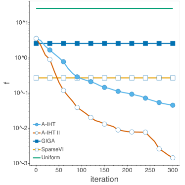
Refer to caption
Figure 5: Convergence results for synthetic Gaussian posterior inference (subsection 5.1) when sparsity setting k=200𝑘200k=200 in the first trial. For GIGA, SparseVI and Uniform, each of the objective function values f𝑓f is calculated by the final output of each algorithms.
Refer to captionRefer to caption
Figure 6: Illustration of true posterior and posterior constructed by A-IHT II after projecting to 2-dimensional plane for synthetic Gaussian posterior inference (Section 5.1). Results at different sparsity level are shown. The ellipses indicate 2σ2𝜎2\sigma-prediction of the posterior distribution, and the black dots represent coreset points selected with their radius denoting the respective weights.

Additional results for experiments in section 5.1 are provided in this section.

From an optimization perspective, one may be curious about the convergence speed of the two proposed algorithms, i.e., A-IHT and Accelerated A-IHT II (Algorithm 2 & 3). The convergence for the two algorithms compared to the solutions by baselines are presented in Figure 5. The x-axis is iteration number for A-IHT and A-IHT II, and the y-axis is the objective function to be minimized, i.e.,

f(w)=yΦw22,𝑓𝑤superscriptsubscriptnorm𝑦Φ𝑤22\displaystyle f(w)=\|y-\Phi w\|_{2}^{2}, (107)

where y=i=1ng^i𝑦superscriptsubscript𝑖1𝑛subscript^𝑔𝑖y=\sum_{i=1}^{n}\hat{g}_{i} and Φ=[g^1,,g^n]Φsubscript^𝑔1subscript^𝑔𝑛\Phi=[\hat{g}_{1},\dots,\hat{g}_{n}].

The two IHT algorithms’ fast convergence speed reflects what our theory suggests. They surpass GIGA within about 30 iterations, and surpass SparseVI within 50 iterations (A-IHT II) and within 100 iterations (A-IHT), respectively. Although we should note that the objective function which SparseVI minimizes is reverse KL divergence instead of l2subscript𝑙2l_{2} distance, the two IHT algorithms can achieve much better solutions when considering KL divergence as well, as shown in Figure 1. Moreover, the tendency of a further decrease in objective value is still observed for the two IHT algorithms at 300thsuperscript300𝑡300^{th} iteration.

Illustration of the coresets constructed by A-IHT II in the first trial after projecting to 2D is presented in Figure 6.

Appendix F Additional Results for Radial Basis Regression
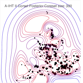
Refer to captionRefer to captionRefer to caption
Figure 7: Experiments on Bayesian radial basis function regression in the first four random trials out of ten trails, where coreset sparsity setting k=300𝑘300k=300. Coreset points are presented as black dots, with their radius indicating assigned weights. Posterior constructed by Accelerated IHT II (left) shows almost exact contours as the true posterior distribution (middle), while posterior constructed by SparseVI (right) shows deviated contours from the true posterior distribution.

In this section, we provide additional experimental results of posterior contours for the radial basis regression experiment (section 5.2).

We plot the posterior contours for both the true posterior and coreset posterior when sparsity level k=300𝑘300k=300 in the first four random trials out of ten trials. The coreset posterior constructed by our Algorithm 3 recovers the true posterior almost exactly, unlike SparseVI. Results are shown in Figure 7.

Appendix G Details and Extensive Results of the Bayesian Logistic and Poisson Regression Experiments
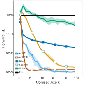
Refer to captionRefer to captionRefer to caption

(a) synthetic dataset for logistic regression

Refer to captionRefer to captionRefer to caption

(b) phishing dataset for logistic regression

Refer to captionRefer to captionRefer to caption

(c) chemical reactivities dataset for logistic regression

Figure 8: Bayesian coreset construction for logistic regression (LR) using the three different datasets. All the algorithms are run 20 times, and the median as well as the interval of 35thsuperscript35𝑡35^{th} and 65thsuperscript65𝑡65^{th} percentile, indicated as the shaded area, are reported. Different maximal coreset size k𝑘k is tested from 111 to 100100100. Forward KL (left) and reverse KL (middle) divergence between estimated true posterior and coreset posterior indicate the quality of the constructed coreset. The smaller the KL divergence, the better the coreset is. The running time for each algorithm is also recorded (right).
Refer to captionRefer to captionRefer to caption

(a) synthetic dataset for Poisson regression

Refer to captionRefer to captionRefer to caption

(b) biketrips dataset for Poisson regression

Refer to captionRefer to captionRefer to caption

(c) airportdelays dataset for Poisson regression

Figure 9: Bayesian coreset construction for Poisson regression (PR) using the three different datasets. All the algorithms are run 20 times, and the median as well as the interval of 35thsuperscript35𝑡35^{th} and 65thsuperscript65𝑡65^{th} percentile, indicated as the shaded area, are reported. Different maximal coreset size k𝑘k is tested from 111 to 100100100. Forward KL (left) and reverse KL (middle) divergence between estimated true posterior and coreset posterior indicate the quality of the constructed coreset. The smaller the KL divergence, the better the coreset is. The running time for each algorithms is also recorded (right).

We consider how IHT performs when used in real applications where the closed-form expressions are unattainable. As the true posterior is unknown, a Laplace approximation is used for GIGA and IHT to derive the finite projection of the distribution, i.e., g^isubscript^𝑔𝑖\hat{g}_{i}. Further, Monte Carlo sampling is needed to derive gradients of DKLsubscript𝐷KLD_{\text{KL}} for SparseVI. We compare different algorithms estimating the posterior distribution for logistic regression and Poisson regression. The reverse KL and forward KL between the coreset posterior and true posterior are estimated using another Laplace approximation. The experiment was proposed by Campbell & Broderick (2019), and is used in (Campbell & Broderick, 2018) (GIGA) and (Campbell & Beronov, 2019) (SparseVI). The experimental settings for each baseline algorithms are set following their original settings for this experiment. In addition, we conduct additional experiments using a stochastic gradient estimator or using an alternative evaluation for coreset quality.

For logistic regression, given a dataset {(xn,yn)D×{1,1}i[N]}conditional-setsubscript𝑥𝑛subscript𝑦𝑛superscript𝐷11𝑖delimited-[]𝑁\{(x_{n},y_{n})\in\mathbb{R}^{D}\times\{1,-1\}\mid i\in[N]\}, we aim to infer θD+1𝜃superscript𝐷1\theta\in\mathbb{R}^{D+1} based on the model:

ynxn,θBern(11+eznθ),similar-toconditionalsubscript𝑦𝑛subscript𝑥𝑛𝜃Bern11superscript𝑒superscriptsubscript𝑧𝑛top𝜃\displaystyle y_{n}\mid x_{n},\theta\sim\text{Bern}\left(\frac{1}{1+e^{-z_{n}^{\top}\theta}}\right), (108)

where zn=[xn,1]subscript𝑧𝑛superscriptsuperscriptsubscript𝑥𝑛top1topz_{n}=[x_{n}^{\top},1]^{\top}. Three datasets are used for logistic regression. The synthetic dataset for logistic regression consists of data xnsubscript𝑥𝑛x_{n} sampled i.i.d. from standard normal distribution 𝒩(0,I)𝒩0𝐼{\mathcal{N}}(0,I), and label ynsubscript𝑦𝑛y_{n} sampled from Bernoulli distribution conditioned on xnsubscript𝑥𝑛x_{n} and θ=[3,3,0]𝜃superscript330top\theta=[3,3,0]^{\top}. The original phishing dataset444https://www.csie.ntu.edu.tw/~cjlin/libsvmtools/datasets/binary.html consists of N=11055𝑁11055N=11055 data points with dimension D=68𝐷68D=68. The phishing dataset used in this experiment is preprocessed (Campbell & Beronov, 2019) via principle component analysis to project each data points to dimension of D=10𝐷10D=10 to mitigate high computation by SparseVI. The original chemical reactivities dataset555http://komarix.org/ac/ds has N=26733𝑁26733N=26733 data points with dimension D=10𝐷10D=10. We uniformly sub-sample N=500𝑁500N=500 data points from each datasets for this experiment, due to the high computation cost of SparseVI.
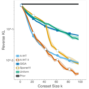
For Poisson regression, given {(xn,yn)D×i[N]}conditional-setsubscript𝑥𝑛subscript𝑦𝑛superscript𝐷𝑖delimited-[]𝑁\{(x_{n},y_{n})\in\mathbb{R}^{D}\times\mathbb{N}\mid i\in[N]\}, we aim to infer θD+1𝜃superscript𝐷1\theta\in\mathbb{R}^{D+1} from model

ynxn,θPoiss(log(1+eznθ)),similar-toconditionalsubscript𝑦𝑛subscript𝑥𝑛𝜃Poiss1superscript𝑒superscriptsubscript𝑧𝑛top𝜃\displaystyle y_{n}\mid x_{n},\theta\sim\text{Poiss}\left(\log\left(1+e^{-z_{n}^{\top}\theta}\right)\right), (109)

where zn=[xn,1]subscript𝑧𝑛superscriptsuperscriptsubscript𝑥𝑛top1topz_{n}=[x_{n}^{\top},1]^{\top}. Three other datasets are used for Poisson regression: the synthetic dataset for Poisson regression consists of data xnsubscript𝑥𝑛x_{n} sampled i.i.d. from a standard normal distribution 𝒩(0,1)𝒩01{\mathcal{N}}(0,1), and target ynsubscript𝑦𝑛y_{n} sampled from Poisson distribution conditioned on xnsubscript𝑥𝑛x_{n} and θ=[1,0]𝜃superscript10top\theta=[1,0]^{\top}. The biketrips dataset666http://archive.ics.uci.edu/ml/datasets/Bike+Sharing+Dataset consists of N=17386𝑁17386N=17386 data points with dimension D=8𝐷8D=8. The airportdelays dataset777The airportdelays dataset was constructed (Campbell & Broderick, 2019) by combining flight delay data (http://stat-computing.org/dataexpo/2009/the-data.html) and weather data (https://www.wunderground.com/history/.). has N=7580𝑁7580N=7580 data points with dimension D=15𝐷15D=15. Same as logistic regression, we uniformly sub-sample N=500𝑁500N=500 data points from each datasets for this experiment.

The comparison of the algorithms for Bayesian coreset construction for logistic regression are shown in Figure 8, and Bayesian coreset construction for Poisson regression are shown in Figure 9. The left column shows forward KL divergence given sparsity setting k𝑘k, the middle column shows reverse KL divergence, and the right column presents the running time for corset construction for each algorithm.

It is observed that A-IHT and A-IHT II achieve state-of-the-art performance. The IHT algorithms often obtain coresets with smaller KL than GIGA and SparseVI, with computing time comparable to GIGA, significantly less than SparseVI. The experiments indicate that IHT outperforms the previous methods, improving the trade-off between accuracy and performance.

The results on large-scale datasets have been presented in the Figure 4 in the main paper. Next, we present two additional sets of experiments that are omitted in the main paper.

Stochastic Gradient Estimator. For large-scale datasets, it is often necessary to “batch" the algorithms. IHT can be easily batched by replacing the gradient with a stochastic gradient estimator that only a batch of data in each iteration.

Recall that for IHT the gradient of the objective function f(w)=yΦw2𝑓𝑤superscriptnorm𝑦Φ𝑤2f(w)=\|y-\Phi w\|^{2} is f(w)=2Φ(Φwy)𝑓𝑤2superscriptΦtopΦ𝑤𝑦\nabla f(w)=2\Phi^{\top}(\Phi w-y), where ΦS×nΦsuperscript𝑆𝑛\Phi\in{\mathbb{R}}^{S\times n}. As we introduced in section 2, S𝑆S is the number of samples θπ^similar-to𝜃^𝜋\theta\sim\hat{\pi}, and n𝑛n is the number of data. Thus, we can form a unbiased gradient estimator as

g~(w)=2Γ1Φ(ΦΓ2wy),~𝑔𝑤2superscriptsubscriptΓ1topsuperscriptΦtopΦsubscriptΓ2𝑤𝑦\displaystyle\tilde{g}(w)=2\Gamma_{1}^{\top}\Phi^{\top}(\Phi\Gamma_{2}w-y), (110)

where Γ1,Γ2n×nsubscriptΓ1subscriptΓ2superscript𝑛𝑛\Gamma_{1},\Gamma_{2}\in{\mathbb{R}}^{n\times n} are i.i.d sampled from a distribution πΓsubscript𝜋Γ\pi_{\Gamma} with 𝔼Γ1πΓ[Γ1]=𝔼Γ2πΓ[Γ2]=Isubscript𝔼similar-tosubscriptΓ1subscript𝜋Γdelimited-[]subscriptΓ1subscript𝔼similar-tosubscriptΓ2subscript𝜋Γdelimited-[]subscriptΓ2𝐼\mathbb{E}_{\Gamma_{1}\sim\pi_{\Gamma}}[\Gamma_{1}]=\mathbb{E}_{\Gamma_{2}\sim\pi_{\Gamma}}[\Gamma_{2}]=I, where In×n𝐼superscript𝑛𝑛I\in{\mathbb{R}}^{n\times n} is the identity matrix. Therefore,

𝔼g~(w)=2(𝔼Γ1)Φ(Φ𝔼Γ2wy)=2IΦ(ΦIwy)=f(w),𝔼~𝑔𝑤2superscript𝔼subscriptΓ1topsuperscriptΦtopΦ𝔼subscriptΓ2𝑤𝑦2𝐼superscriptΦtopΦ𝐼𝑤𝑦𝑓𝑤\displaystyle\mathbb{E}\tilde{g}(w)=2(\mathbb{E}\Gamma_{1})^{\top}\Phi^{\top}(\Phi\mathbb{E}\Gamma_{2}w-y)=2I\Phi^{\top}(\Phi Iw-y)=\nabla f(w), (111)

showing that g~(w)~𝑔𝑤\tilde{g}(w) is an unbiased estimator of f(w)𝑓𝑤\nabla f(w).

For example, we can form the estimator using a batch of data with batch size B𝐵B by letting Γ1,Γ2subscriptΓ1subscriptΓ2\Gamma_{1},\Gamma_{2} be random matrices as randomly setting nB𝑛𝐵n-B rows of nBI𝑛𝐵𝐼\tfrac{n}{B}I be zero. Equivalently, it is the same as randomly picking B𝐵B columns of ΦΦ\Phi, setting the rest columns be zero, and scale the matrix by n/B𝑛𝐵n/B. Noting that each column of ΦΦ\Phi corresponds to each of the n𝑛n data points, this operation is essentially to approximate ΦΦ\Phi using a batch of data with batch size B𝐵B, and thus it approximates the gradient using a batch of a data.

We test how Algorithm 2 performs on the Bayesian logistic regression and Poisson regression using the stochastic estimator with batch size B=n/5𝐵𝑛5B=n/5. All of the experimental settings are the same as what we have introduced in this section. As a summary of both forward FL and reverse KL, we use the symmetrized KL (i.e., the sum of forward KL and reverse KL) as the evaluation metric for coreset quality. The results are shown in Figure 10. It is observed that A-IHT with the stochastic gradient estimator (A-IHT batch grad.) performs comparably to the A-IHT. We note that the batched version of A-IHT can be improved by increasing its maximal number of iterations, i.e., optimization with stochastic gradient needs more iterations to converge, or using a better batch gradient estimator. Theoretical study on accelerated IHT with approximated gradients is still an open question to the best of our knowledge. Further research on accelerated IHT with stochastic gradients is an interesting future work.

Refer to caption

synthetic dataset for logistic regression
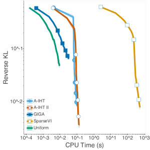
Refer to caption

phishing dataset for logistic regression
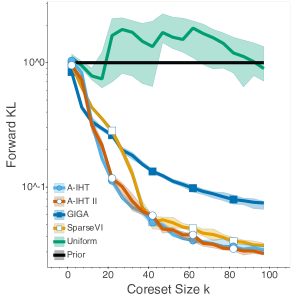
Refer to caption

chemical reactivities dataset for logistic regression

Refer to caption

synthetic dataset for Poisson regression

Refer to caption

biketrips dataset for Poisson regression

Refer to caption

airportdelays dataset for Poisson regression

Figure 10: Bayesian coreset construction for logistic regression and Poisson regression using the six different datasets. All the algorithms are run 20 times, and the median as well as the interval of 35thsuperscript35𝑡35^{th} and 65thsuperscript65𝑡65^{th} percentile, indicated as the shaded area, are reported. Different maximal coreset size k𝑘k is tested from 111 to 100100100. Symmetrized KL divergence between estimated true posterior and coreset posterior indicate the quality of the constructed coreset. The smaller the KL divergence, the better the coreset is.

2subscript2\ell_{2}-distance Evaluation of Coreset Quality. In the previous experiments in the subsection, the coreset quality is evaluated by approximating the KL divergence between the full-dataset posterior and coreset posterior. As an alternative way to measure the coreset quality, we measure the 2subscript2\ell_{2}-distance between the maximum-a-posteriori (MAP) estimation of the full-dataset posterior and coreset posterior. The results are shown in Figure 11. It is observed that the two IHT algorithms usually achieve the best results, except that SparseVI achieves the lowest 2subscript2\ell_{2}-distance on two datasets. However, SparseVI costs ×104absentsuperscript104\times 10^{4} more time than IHT and GIGA.

Refer to caption

synthetic dataset for logistic regression

Refer to caption

phishing dataset for logistic regression
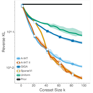
Refer to caption

chemical reactivities dataset for logistic regression
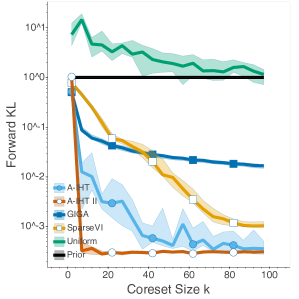
Refer to caption

synthetic dataset for Poisson regression
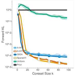
Refer to caption

biketrips dataset for Poisson regression
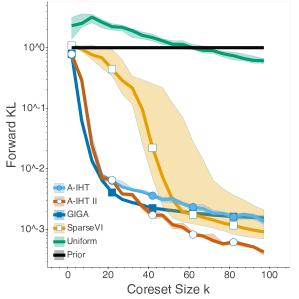
Refer to caption

airportdelays dataset for Poisson regression

Figure 11: Bayesian coreset construction for logistic regression and Poisson regression using the six different datasets. All the algorithms are run 20 times, and the median as well as the interval of 35thsuperscript35𝑡35^{th} and 65thsuperscript65𝑡65^{th} percentile, indicated as the shaded area, are reported. Different maximal coreset size k𝑘k is tested from 111 to 100100100. 2subscript2\ell_{2}-distance between the MAP estimators of the full-dataset posterior and coreset posterior indicate the quality of the constructed coreset. The smaller the 2subscript2\ell_{2}-distance, the better the coreset is.