ConFoc: Content-Focus Protection Against
Trojan Attacks on Neural Networks
Abstract
Deep Neural Networks (DNNs) have been applied successfully in computer vision. However, their wide adoption in image-related applications is threatened by their vulnerability to trojan attacks. These attacks insert some misbehavior at training using samples with a mark or trigger, which is exploited at inference or testing time. In this work, we analyze the composition of the features learned by DNNs at training. We identify that they, including those related to the inserted triggers, contain both content (semantic information) and style (texture information), which are recognized as a whole by DNNs at testing time. We then propose a novel defensive technique against trojan attacks, in which DNNs are taught to disregard the styles of inputs and focus on their content only to mitigate the effect of triggers during the classification. The generic applicability of the approach is demonstrated in the context of a traffic sign and a face recognition application. Each of them is exposed to a different attack with a variety of triggers. Results show that the method reduces the attack success rate significantly to values in all the tested attacks while keeping as well as improving the initial accuracy of the models when processing both benign and adversarial data.
I Introduction
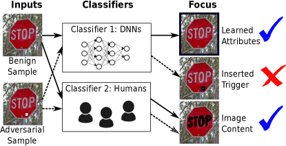
Advances in artificial intelligence have positioned Deep Neural Networks (DNNs) as one of the main algorithms currently used for machine learning. They have successfully been applied to solve problems in multiple areas such as natural language processing [1] and computer vision [2]. For the later case, their success have been proved in classification-based applications like object detection [3] and scene [4], face [5], and traffic sign recognition [6]. Despite being broadly used in these applications, the wide adoption of DNNs in real-world missions is still threatened by their ingrained security concerns (e.g., lack of integrity check mechanisms and their uncertain black-box nature [7, 8]), which make them vulnerable to trojan or backdoor attacks (hereinafter trojan attacks) [9, 10, 11, 12].
Trojan attacks against DNNs occur at training time and are later exploited during testing. To execute them, adversaries slightly change original models at training by either poisoning or retraining them with adversarial samples. These adversarial samples are characterized by having a trigger (e.g., a set of pixels with specific values in the computer vision scenario) and a label chosen by the adversary (target class). The ultimate goal of the attack is inducing misbehavior at testing time as any input with the trigger is misclassified to the target class. These attacks represent a powerful threat because it is difficult to determine whether a model is compromised. Inputs without the trigger (benign samples) are normally classified [13] and deployed triggers can be designed to be unnoticeable (e.g., triggers may look like black spots by dirt in cameras) [14].
The potential of these attacks is illustrated in the context of self-driving cars. These vehicles capture pictures of objects on the streets and process them without adversaries editing the captured images. If these cars were using a compromised model, adversaries could induce the misclassification of street objects by simply stamping marks (e.g., stickers) on them, which would act as triggers when images are captured. Attackers might cause harm if stop signs are misclassified to speed signs. As DNNs are incorporated by companies such as Google and Uber in their self-driving solutions and are also used in other critical applications (e.g., authentication via face recognition of the Apple IPhone X) [14], protecting against trojan attacks on DNNs is an important problem to solve.
Previous defensive strategies either harden DNNs by increasing their robustness against adversarial samples [12, 13, 7] or detect adversarial inputs at testing time [12, 7, 14, 8]. This research is in the former category. Some existing techniques in this category assume access to a large training dataset to train auxiliar models [12]. Others reduce the attack effectiveness at the cost of accuracy by fine-tuning compromised models after pruning a number of neurons [13]. A state-of-the-art model hardening technique, called Neural Cleanse [7], proposed an improved solution. It assumes access to a small training set and fine-tunes models with images including reverse-engineered triggers. This technique significantly reduces the attack success rate. However, based on our experiments in Section VI-C, it does not improve the accuracy of the models enough when processing adversarial samples in some of the tested attacks, limiting its generic applicability.
Images are comprised of both content and style. Content refers to the shapes of objects or semantic information of images, while style refers to their colors or texture information [15]. In this work, we identify that the features learned by DNNs, including those related to triggers, are also formed by a combination of content and style, which are recognized as a whole by DNNs at testing time. Our hypothesis is that it is possible to teach models to focus on content only so that they resemble better the human reasoning during the classification to avoid exploitation (Figure 1a). Based on this, we devised a content-focus healing procedure, called , which takes a trojaned model and produces a healed version of it. assumes access to a small benign training set (healing set) and generates from each sample in it a variety of new samples with the same content, but different styles. These samples are used in a twofold healing strategy in which models: (1) forget trigger-related features as they are fine-tuned with original and styled benign samples only and (2) improve their accuracy with both benign and adversarial data due to the data augmentation achieved with multiple styles. As the only common characteristic among the original and styled samples is the content itself, models learn to focus on it. At testing, inputs can be classified with either its original or a random style because styles are ignored.
overcomes the limitations of previous work [12, 13, 7] as it is characterized by: (1) being generic and effective against different trojan attacks, (2) functioning without prior knowledge of the trigger, (3) depending on a small training set, and (4) avoiding neuron pruning (which affect performance). Our main contributions are listed below:
-
•
We analyze the composition of the features learned by DNNs and identify that they have both content and style. We demonstrate that trojan attacks can be countered by making models focus on content only.
-
•
We built a prototype [16] and evaluate with a variety of applications, including a traffic sign recognition system implemented in Resnet34 [17] with the GTSRB dataset [18] and a face recognition system (VGG-Face [19]). Each application is exposed to a different type of trojan attack executed with a variety of triggers. The former is tested against the trojan attack BadNets [9], while the latter with Trojaning Attack [11]. Compared to the state-of-the-art [7], shows good results against both attacks, whereas the other technique does it in one of the cases.
-
•
is agnostic to the image classification application for which models are trained, with the benefit that it can be applied equally to any model (trojaned or not) without impacting its classification performance.
-
•
To our knowledge, we are the first establishing the importance of evaluating defensive methods against trojan attacks with the correct metrics: (1) accuracy with benign data, (2) accuracy with adversarial data, and (3) attack success rate or ASR (percentage of adversarial samples classified to the target class). This is crucial because it is possible to have models with both low ASR and low accuracy with adversarial data, on which adversaries can still conduct an untargeted attack by triggering the misclassification of adversarial samples to a random rather than to a the target class.
Our work provides a new model hardening technique that reduces the sensitivity of DNNs to inserted triggers. Although the interpretability of DNNs is out of our scope, represents an valuable tool for defenders against trojan attacks.
II Threat Model and Overview
II-A Threat Model
We assume an adaptive attacker that gains access to an original non-trojaned model and inserts a trojan into it before the model reaches the final user. The adaptive attacker is knowledgable about the approach and is able to infect models with styled adversarial samples to mitigate the healing effect. Adversaries can achieve the attack by either poisoning the training dataset (at training time) or retraining the model (after the training period) before reaching the final user. That is, adversaries have the capabilities of an insider threat who can efficiently poison the data used to train the victim model. Also, adversaries have the ability to act as a man-in-the-middle, who intercepts the original non-infected model, retrains it to insert the trojan, and then tricks the final users to use the resulting trojaned model. The later assumption is a plausible scenario as the most accurate neural network architectures tend to be either deeper or wider [17, 20]. Whereby, transfer learning in DNNs [21, 22] is a common practice and pre-trained models are often downloaded from public sites without the proper integrity check[12]. Upon getting a model (either trojaned or not), final users take them through the method. We assume adversaries cannot interfere in this process. At testing, adversaries endeavor to provide adversarial inputs to the models without being able to modify them anymore.
II-B Overview
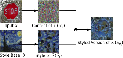
A compromised model is referred to as a trojaned model (). In order to heal an , retrains it with a small set of samples and their strategically transformed variants until the model learns to make the classification based on the content of images. Our technique is founded on the concept of image style transfer [15], which is applied for first time in a security setting to generate the training samples used in the healing process. Figure 1b shows this concept. Images can be separated in content and style, and it is possible to transfer the style of one image to another. Under the assumption of holding a small healing set of benign samples and a set of style base images , extracts from them their image content and styles respectively. The styles are transferred to the content images to generate the set of styled images . During the healing process, each benign sample , its content image , and corresponding styled images are used as training data. Our intuition is that models learn to focus on the content as it is the only common characteristic among these samples. The goal is to reduce the sensitivity of DNNs to trigger-related features during the process.
Any model resulting from the healing process is referred to as a healed model (). At inference time, any input is classified by , which focus on its content only. The input can optionally be transformed to a particular styled version using any chosen style base image before being classified because its style is ignored in the process.
Limitations. We summarize three main limitations. First, relies on having access to a healing dataset. Although this is a challenging requirement, our technique is proved to be effective with small datasets around 1.67% of the original training set size. Second, imposes an overhead at testing if inputs are first transformed (optionally) to change their styles. Likewise, our method requires some time to generate the content and styled images used in the healing process. These overheads are limited, however, because the image transformation takes only a few milliseconds and the healing process occurs offline. Finally, like previous techniques [12, 13, 7], we assume adversaries cannot run attacks (e.g., poisoning) during the healing process. This is a reasonable assumption that does not abate our contribution to methods that remove trojans without impacting the performance of DNNs.
III Background and Related Work
III-A Deep Neural Networks
A DNN can be interpreted as a parameterized function , which maps an -dimensional input into one of classes. The output of the DNN is a -dimensional tensor representing the probability distribution of the classes. That is, the element of the output represents the probability that input belongs to the class .
Specifically, a DNN is a structured feed-forward network in which each corresponds to a layer of the structure. A layer outputs a tensor whose elements are called neurons or activations. Activations are obtained in a sequential process. Each layer applies a linear transformation to the activations of the previous layer followed by a non-linear operation as follows: . The output of () is referred to as output activations, while the input () as input activations. Outputs of middle layers are called hidden activations. The elements and are tensors corresponding to the parameters and are called weights and bias respectively. The component of the equation is the non-linear operation of the layer . There are multiple non-linear operations, each with different effects in their outputs. Some of them are sigmoid, hyperbolic tangent, Rectified Linear Unit (ReLU) and Leaky ReLU [23, 24].
A DNN is trained with a set of input-output pairs provided by the trainers, where is the input and the true label or class of . Trainers define a loss function , which estimates the difference between the real label and the predicted class . The objective of the training process is minimizing the loss function by iteratively updating the parameters through backpropagation [25]. In essence, backpropagation is a gradient descent technique that estimates the derivatives of the loss function with respect to each parameter. These derivatives determine how much each parameter varies and in what direction. The training process is controlled by trainer-specified hyper-parameters such as learning rate, number of layers in the model, and number of activations and non-linear function in each layer.
During testing, a trained DNN receives an unseen input , produces an output , and assign to the class .
This paper focuses on Convolutional Neural Networks (CNNs) trained for image classification tasks. CNNs are a type of DNNs characterized by being: (1) sparse as many of their weights are zero, and (2) especially structured as neuron values depend on some related neurons of previous layers [13].
III-B Trojan Attacks: Assumptions, Definition and Scope
Assumptions. Trojan attacks consist of adding semantically consistent patterns to training inputs until DNNs learn those patterns and recognize them to belong to either a specific or a set of target classes chosen by the adversary [14]. Several approaches can be followed to insert a chosen pattern or trigger into the training data to achieve the trojaned misbehavior. The difference among them lies on the strategy applied to generate the adversarial samples, the objective of the misclassification, and the applicability of the attack. This research aims to feature a solution to counter trojan attacks that comply with the following conditions:
-
Adversarial samples include an unknown pattern (or trigger) inserted into the victim DNNs during training.
-
Benign samples are normally classified by compromised models.
-
Both benign and adversarial samples are assumed to belong to the same distribution. This implies that triggers, which might be perceptible, do not override the interesting object in the image to be classified.
-
Adversarial testing samples are generated without any manipulation or further processing after the image is captured. It implies adversaries do not have access to the model at inference or testing time.
Trojan attack definition. Assuming an original non-trojaned model trained with a set of benign samples . Given a correctly classified benign input to the class , a labeling function , and a target class chosen by the adversary, the input is an adversarial sample at training time if:
| (1) |
Now, let be the set of adversarial samples generated following Equation 1 and the trojaned version resulting from training the model with both and . At testing time, given be a benign input correctly classified to the class , an input is an adversarial sample if:
| (2) |
| (3) |
In Equation 1 and Equation 2, represents the changes caused to sample by the addition of a trigger (). These changes might be obvious to humans as shown in the example in the left side of Figure 1a. Despite the possible obvious difference between benign and adversarial samples, for any benign sample at inference time, it is also assumed that since as established in Equation 3 and users are unaware of the triggers used in the attack ( and ). The labeling function in Equation 1 is controlled by the adversary at training time and is used to assign the chosen target class as label of the adversarial sample . Equation 2 establishes that at testing, a sample (not originally belonging to the class ) is considered adversarial if it contains the trigger and is classified by the trojaned model to the target class . Triggers can be added without manipulating testing samples by, for example, attaching a sticker to the object to be classified before capturing its image ().
In summary, trojaned models closely classify benign inputs as non-trojaned models, thwarting the ability to determine whether a given model has an inserted trojan. Thereby, in trojan attacks it is assumed final users are deemed unaware of the committed attack and use the trojaned model under the believe the model is .
Scope. We evaluate our method against two trojan attacks that comply with conditions -: BadNets [9], and Trojaning Attack [11]. We do not consider trojan attacks with weak and strong assumptions about the capabilities of defenders and attackers, respectively. One example is the attack that poisons the training data using an instance of class A and a set of n variants of it (created by adding random noise) labeled as B in order to misclassify inputs in A to B [10]. As benign inputs themselves are used to insert the trojan, defenders can detect the misbehavior by observing the misclassified samples (low defensive capability assumed). Another example is the attack that inserts trojans by blending benign inputs with images containing specific patterns that function as triggers [10]. In this case, adversaries manipulate the inputs during both training and testing (high offensive capability assumed).
Other threats known as adversarial sample attacks [26, 27, 28, 29, 30, 31] and adversarial patch attacks (and variants) [32, 33] (and hence their counter measures [34, 35, 36, 37, 38, 39, 40, 41, 42, 43] ) are also out of the scope of this paper. These attacks cause misclassification as well, but the assumptions and patterns added to inputs are different from those in trojan attacks. These attack variations are executed at testing time only with samples generated via gradient descent using the victim models in the process. [14].
III-C Prior Work on Trojan Attacks
| Technique | Training Dataset | Modify Model | Knowledge of Trigger | Rigorously tested |
| Retraining [12] | Large | No | Not required | No |
| Encoder [12] | Large | No | Not required | No |
| Fine-Pruning [13] | Small | Yes | Not required | Yes |
| Neural Cleanse (Pruning) [7] | Small | Yes | Required | Yes |
| Neural Cleanse (Unlearning) [7] | Small | No | Required | Yes |
| [this study] | Small | No | Not required | Yes |
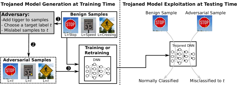
Gu et al. [9] introduced a trojan attack technique called BadNets, which inserts a trojan into DNNs by poisoning the training dataset. Figure 2 illustrates the attack in the context of a traffic sign recognition system. The attack is executed in two phases: a trojaned model generation phase and a model exploitation phase. In the former, adversaries follow three steps. Step1, adversaries sample a small set of images from the training dataset. Step2, attackers choose a target class t and a trigger to create the adversarial samples. Adversarial samples are created by adding the chosen pattern to the selected samples and changing the labels of the samples to the class t. Step 3, adversaries feed the generated adversarial samples into the model during the training process, guaranteeing the pattern is recognized by the model to belong to the class t.
The second phase is shown in the right side of the figure. The benign sample is normally classified, whereas the corresponding adversarial sample is misclassified to the class t. The efficiency of BadNets was proved over the MNIST dataset [44] and the traffic sign object detection and recognition network Faster-RCNN (F-RCNN) [45] with an ASR above 90%.
A more sophisticated trojan technique called Trojaning Attack was presented by Liu et al. in [11]. Three main variations are added to the strategy followed by this technique in comparison to BadNets [9]. First, the attack is conducted by retraining a pre-trained model instead of poisoning the training data. Second, the adversarial training samples used for retraining are obtained via a reverse-engineering process rather than being generated from real benign training samples. Finally, the trigger used in the attack is not arbitrarily chosen, but rather fine-tuned to maximize the activations of some chosen internal neurons. Reverse-engineered images refer to images whose pixels were tuned via gradient descent to be classified to a specific class. Triggers were also obtained via gradient descent using a loss function defined with respect to the activations of a specific layer . Their pixels are tuned to induce maximum response in certain neurons in . During the retraining process with benign and adversarial reverse-engineered images, only the layers following layer are fine-tuned. The attack was demonstrated over the VGG-Face model [19] with an ASR greater than 98%.
III-D Existing Defensive Techniques Against Trojan Attacks
Fine-Prunning [13] is a model-hardening technique that identifies trigger-related neurons and removes them to eliminate their effect. The efficiency of the method suffers for the high redundancy among internal neurons. Wan et al. [7] proved that despite the fact that only 1% of the output neurons are activated by certain region (set of pixels) of an input image, more than 30% of the total output neurons need to be removed to eliminate the effect of that region on the classification process. This implies a high cost in the performance of the model. In light of this observation, unlike Fine-Prunning, does not modify the architecture of models.
Liu eat al. [12] presented three methods against trojan attacks tested over the MINST dataset [44]. First, a technique to detect adversarial samples by comparing the outputs of the victim model with the outputs of binary models based on Decision Trees (DTs) [46] and Support Vector Machines (SMV) [47] algorithms. Second, a model hardening technique that fine-tunes the victim model with a set of benign samples. Although the method reduces the attack, it also has an impact in the accuracy of model [7]. Finally, a model hardening approach in which an encoder is inserted between the input and the model. This encoder is trained with benign samples only and is used to filter out samples at testing by compressing their features, and decompressing them again to have samples that do not include the trigger before being classified. The three described methods assume access to a training set without any restriction to its size. , in contrast, requires a small set of less than or equal to 10% of the original training set size.
Ma et al. [14] attributes trojan attacks to the uncertain nature of DNNs and identify two main attack channels exploited by adversaries. First, a provenance channel exploited when adversarial changes are added to inputs to alter the path of active neurons in the model from input through all the middle layers until the output to achieve misclassification. Second, an activation value distribution channel, in which the path of activate neurons from input to output remains the same for both benign and adversarial inputs, but with different value distributions for these two types of inputs. The authors developed a technique that extracts the invariants of these two channels and use them to detect adversarial samples.
Tao et al. [8] proposed an adversarial input detection technique that finds a bidirectional relationships between neurons and image attributes easily recognized by humans (e.g., eyes, nose, etc.) for face recognition systems. A parallel model is created from the original model by strengthening these neurons while weakening others. At testing time, any input is passed to both models and considered adversarial in case of a classification mismatch. Although this work is proved to be effective, it assumes attributes on which humans focus on to make the decisions are known in advance. , disregards this assumption as it lets models extract the content of images on their own through the healing process.
Wang et al. [7] presents Neural Cleanse, a strategy with three main defensive goals: (1) determining whether a given model has a trojan inserted, (2) if so, reverse-engineering the trigger, and (3) mitigating the attack through complementary defensive methods: Patching DNN Via Neuron Pruning and Patching DNN Via Unlearning. Authors show that the former does not perform as well against Trojaning Attack [11] as it does against BadNets [9]. The latter is proved to be effective against both attacks, but only for targeted modalities as the performance is measured using accuracy with benign data and ASR only. In addition to these metrics, is tested using accuracy with adversarial data, proving its effectiveness against both targeted and untargeted trojan attacks.
falls into the category of model hardening. Hence, we focus on these types of solutions. Table I shows a qualitative comparison with previous techniques in this category.
IV Content-Focus Approach
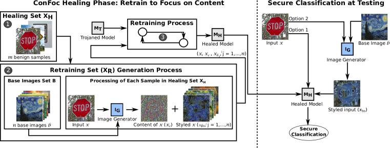
Figure 3 illustrates our content-focus approach () to defend against trojan attacks. The approach is executed in two phases. First, a healing phase (left side of the figure), which takes a trojan model and strategically retrains it to produce a healed model . Second, a secure classification phase at testing time, which uses the produced to classify inputs based on their content or semantic information, mitigating the effect of triggers when processing adversarial samples (right side of the figure.)
The ConFoc healing process assumes defenders have access to a limited number of benign samples from the same distribution as the benign data used during the original training of . The process is completed in three steps. In step 1, a small healing set of of these benign samples is selected. Step 2 is a process that uses the selected healing set and a set of randomly chosen style base images to generate a larger retraining dataset . The process takes each benign sample and passes them to the Image Generator . The generates from each its content and multiple versions of styled images , obtained by transferring the style of each to the content . The retraining dataset comprises each , its content and its corresponding generated styled images. As the only common characteristic among these samples is their content, the final step of the healing process (step 3) is retraining the trojaned model with the set so that the model learns to focus on the content of inputs. The goal is producing a healed model , in which the trojaned misbehavior becomes ineffective and the accuracy is high for both benign and adversarial data.
At testing, a secure classification is achieved by either processing the original input (option 1) or passing it first through the (option 2) to produce a styled version of it using any chosen style base image (not necessarily in ). Either image or is classified by the healed model .
The is a crucial element in . Its main purpose is generating the retraining samples for the healing process and transforming the inputs at testing. It comprises four components: (1) feature extraction, (2) content image generation, (3) style image generation, and (4) styled image generation.
IV-A Feature Extraction
The output of each layer in a DNN model (i.e., neurons or activations) can be thought as internal features of the input. Feature extraction refers to obtaining these outputs (features) when an input sample is processed by a given model.
Our extracts features using a VGG16 model[48] pre-trained with the Imagenet dataset [49]. This model has 16 layers, from which 13 are convolutional (Conv) and 3 are linear (Linear). The convolutional layers are either followed by a ReLU [50] along with a MaxPool2d [51] or just a ReLU layer. More precisely, the convolutional part of VGG16 is compounded by 2 consecutive arrangements of Conv/ReLU/Conv/ReLU/MaxPool2d followed by 3 arrangements of Conv/ReLU/Conv/ReLU/Conv/ReLU/MaxPool2d.
The selection of the proper layers for feature extraction is an important design choice in the generation of content and styled images. The criterion for this selection was identifying the last layer of a consecutive group of layers that does not remove information. As MaxPool2d layers are intended to down-sample an input representation reducing its dimensionality [51], the layers before each of the five MaxPool2d were chosen in an input-to-output order as potential candidates for feature extraction. These layers form the set (with ), which are used by the next three algorithms.
IV-B Content Image Generation
Algorithm 1 shows the procedure followed to generate a content image. It uses gradient descent to find the local minimum of the defined loss function, which is the Mean Square Error (MSE) between the features extracted from one layer of the VGG16 model given two different inputs. One input is a benign sample from which the content will be extracted. The other is a random uniformly generated image . After the random initialization, the algorithm updates the pixel values of using the gradients estimated through the loss function in such a way that the eventual values of the extracted features are close enough for both inputs. We found to provide the best results to generate content.
Algorithm 1 uses five parameters. Parameter denotes one benign input from the available healing set ; denotes the model used for the featured extraction (VGG16 in our case); corresponds to the layer of the model from which features are extracted; represents the penalty term for the loss function used to control how much information is included in the content; and the maximum number of iterations run by the selected optimizer (we chose LGBFS [52]).
Line 1 generates a random image of the same size as the provided input . Line 2 represents the feature extraction function, which can be thought as slicing the model until the indicated layer . Line 3 gets the features or output of layer of model using the function created in line 2 with sample as argument. From line 4 to 10 gradient descent is used to refine the values of the random image created in line 1. Line 5 follows a procedure similar to the one described in line 3. In this case, it extracts the features at layer using the random image as argument of the function . Line 6 estimates the loss value, which is the Mean Square Error (MSE) between the features obtained at layer for input (line 3) and input (line 5). Line 7 estimates the gradients of the loss with respect to the random input . These gradients are used to update the the random image as indicated at line 8.
IV-C Style Image Generation
Although the styles of base images are not used in , the procedure to generate them is an essential part in the generation of styled images. Therefore, a step-by-step description is included in this section. The style of a given image can be obtained following a similar procedure to the one used to generate content images. The main difference lies on the loss function used to estimate the gradients, which is based on Gramian matrices [53]. For a set of vectors the Gramian matrix is a square matrix containing the inner products among the vectors. In the context of the VGG16 model or any DNN, for a particular layer of the model with channels in its output (features), a Gramian matrix can be obtained by first flattening each channel and then estimating the inner product among the resulting vectors.
Algorithm 2 shows the procedure to generate style images. The paramenter represents the image from which the style is extracted; denotes the model used for the extraction; the set of candidate layers for feature extraction; and the maximum number of iterations the optimizer runs. It was a design choice to use all the candidate layers in in the definition of the loss function.
In the algorithm, line 1 generates a random image of the same size as input image . From lines 2 to 6 a function to extract the features of each layer in is created. The features of each layer are extracted (line 5) with the corresponding function (line 4) using image as argument. The extracted features are stored in the empty vector created in line 2. From lines 7 to 16 gradient descent is applied to refine the random image after estimating the value of the loss function. From line 8 to line 11 the functions created in line 4 extract the features of each layer in using the random image as input. The features are stored in the empty vector created in line 8. Line 12 estimates the style-related loss. This loss sums up the MSE of the Gramian matrices of the features extracted in each layer when the random image and the given image are passed as inputs to the model. From line 13 to 14 the gradients are estimated and is updated accordingly.
IV-D Styled Image Generation
This procedure combines the steps followed in Algorithm 1 and Algorithm 2 for content and style images respectively. It includes a new parameter , which is the index of the layer from which to extract the features used for the generation of the content. Lines 2 to 9 extract the features from each layer using image as input to the model. Features from the layer are extracted using image as input (line 7). From lines 10 to 21 the loss for content and the loss for style are combined in one loss that is later used for the estimation of gradients. From line 11 to line 14 features from each layer are extracted using the random image (created in line 1) as input to the model. Line 15 estimates the content-related loss using the features extracted from the layer with input (line 7) and (line 13) as inputs. Line 16 computes the style-related loss using the Gramian matrices of the features extracted when the random image and the style base image are passed as inputs to the model. Line 17 combines the two loss functions in one, which is used to estimate the gradients (line 18) used to update the random image (line 19). For both Algorithm 3 and Algorithm 1, a fixed rule was created to assign values to based on the size of the input.
V Evaluation Setup
We designed a number of experiments to evaluate under the assumption that a non-trojaned model is compromised by an adversary, who inserts a trojan into it to produce a trojaned model . can be thought as a function that takes as input a model (either or ) and produces a healed model . When the input is , is expected to be a model without the trojaned misbehavior. In the case of having as input, is expected to at least keep its accuracy. During the experiments, all the models are fine-tuned with hyper-parameters (e.g., number of epochs, learning rates, etc.) chosen to get the best possible performance. This allows evaluating using different datasets and attacks.
is tested against BadNets [9] and Trojaning Attack [11], executed with different datasets to validate the generality of the approach. The Trojaning Attack is executed with two triggers: square (SQ) and watermark (WM). The latter trigger was chosen to evaluate the effect of having triggers that overlap key features of the objects to be classified (a violation of condition ). Table II summarizes these three attacks. In addition, a comparison between and the state-of-the-art Neural Cleanse [7] is presented along with results of our method when the attacks are conducted with complex triggers.
| Properties | BadNets | Trojaning (SQ) | Trojaning (WM) |
| Example of Adv. Input | |||
| Strategy | Poisoning | Retraining | Retraining |
| Architecture | Resnet34 | VGG-Face | VGG-Face |
| Dataset | GTSRSB | VGG-FAce | VGG-Face |
| No. Classes | 43 | 40 | 40 |
V-A Evaluation Metrics and Testing Sets
Metrics. The success of a trojan attack can be measured based on two aspects. First, the efficiency to keep compromised models having a high accuracy (rate of classification to the true class) when processing benign data. Second, the attack success rate or ASR, which measures how well triggers in adversarial samples activate the misbehavior [11]. As the latter is expected to be high, trojaned models are also characterized by having low accuracy when processing adversarial data. As a compromised model goes through the healing process our method aims to: (1) reduce the ASR to avoid targeted exploits (misclassification to the target class), (2) keep or improve the accuracy when processing benign inputs, and (3) improve the accuracy with adversarial samples to avoid untargeted exploits (misclassification to random classes). These three factors are the metrics used to measure the performance of .
Testing Sets. Experiments are run with two versions of a given testing set: (1) the given benign version to measure accuracy with benign data and (2) its adversarial version to measure accuracy with adversarial data and ASR. The adversarial versions result from adding the trigger to the samples of the given set. The size of the sets are given as a percentage of the original training set used to create the models.
V-B BadNets Attack
Implementation. We conducted the attack against a traffic sign recognition model following the steps described in [9]. The model was built on Resnet34 [17] pre-trained with the Imagenet dataset [49]. The pre-trained model was fine-tuned using the German Traffic Recognition System Benchmarks (GTRSB) dataset [18].
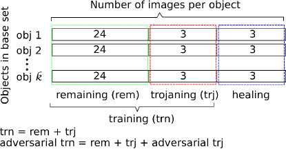
Dataset. GTRSB is a multi-class single-image dataset that contains 39209 colored training images classified in 43 classes (0 to 42), and 12630 labeled testing images. The classes are of traffic sign objects such as stop sign, bicycles crossing, and speed limit 30 km/h. For each physical traffic sign object in the GTRSB training dataset there are actually 30 images. To avoid leakage of information between the data used for training and validation, the GTRSB training dataset was split by objects in two sets: the validation set and the base set. The validation set was formed by taking 10% of the objects (30 images per each) of every class. The other 90% of objects of each class formed the base set. The base set was further split to form the final training, trojaning and healing sets as shown in Figure 4. The split in this case was done based on images. For each particular object in the base set 3 out 30 images were taken for the healing set. Other exclusive 3 images were taken for the trojaning set (trj), leaving 24 images per object in the remaining set (rem). The trojaning set is called adversarial when the chosen trigger is added to its samples and the samples are mislabeled to the chosen target class. The training set (trn) comprises both the remaining and trojaning sets (trn = rem + trj) and is used in the experiments to create the original non-trojaned model . The adversarial training set, on the other hand, comprises the remaining, trojaning, and adversarial trojaning sets (adversarial trn = rem + trj + adversarial trj) and is used to train the trojaned version of referred to as trojaned model .
Testing set. Ten images per class were randomly chosen out of the 12630 available testing samples.
Attack strategy. The adversarial samples were generated by inserting a white square as trigger in the botton right corner of the benign inputs. The size of the square was chosen to be 10% the size of the smallest between the height and width dimensions, and located 5% of this value from the borders. Table II, in row and column 2, shows an adversarial sample with the trigger. Each adversarial sample was labeled with the target class 19, regardless the true class of the samples.
V-C Trojaning Attacks: Square (SQ) and Watermark (WM)
Implementation. For these attacks, was tested against two compromised models provided in [11]. The two models correspond to the same pre-trained face recognition application VGG-Face, infected using two different fine-tuned triggers: square and watermark. As the accuracy of the provided models was relatively low ( 90%) when tested with the original data in [11], we only consider those classes with low rate of misclassification for our experiments. The idea was to have an initial trojaned model with high accuracy when processing benign data. To this end, we randomly selected 40 classes including the taget class (0 or A.J. Buckley). This experimental design choice does not affect the high ASR and low accuracy with adversarial samples of the models.
Dataset. The original VGG-Face dataset includes images of classes (1000 images per class). Currently, no all the images are available and among them there are a significant amount of mislabeled cases. Namely, cases in which random images or images of a person A are labeled as person B. For our healing set, we chose 50 out of the available images for each of the selected 40 classes. This represents 5% of the size of the original dataset. To reduce the noise caused by the mislabeled cases, only images with frontal pose faces were selected. We then manually cleaned the resulting dataset by removing obvious mislabeled samples. The authors of the attack [11] used two sets for testing, being one of them extracted from the VGG-Face dataset. This testing set (referred to by the authors as original dataset) is compound of one image per class, and was used to measure the accuracy and ASR of the model. The other testing set was called external dataset and was extracted from the LFW dataset [54]. The images in this set do not necessarily belog to any of the classes, and were used to measure the ASR only. As one of our main goals is to measure the performance of models with the three metrics listed in Section V-A, we conducted the experiments with a variation of the original dataset only. This ensured a fair comparison with results obtained in previous work.
| Acronym | Description |
| Set of style base images used in the healing process. | |
| Set of style base images not used in the healing process such that . | |
| Indicates that the model was evaluated with the original testing set (i.e., without transforming the inputs). | |
| Indicates that the model was evaluated with styled versions of the testing set (i.e., inputs are transformed). | |
| Original non-trojaned model. | |
| Trojaned model. | |
| Healed model retrained with the retraining set . is compound of the healing set only. | |
| Healed model retrained with the retraining set . comprises the healing set , and its corresponding content images (via Algorithm 1). | |
| Healed model retrained with the retraining set . is formed by the healing set , its content images (via Algorithm 1), and the styled images generated with the first style base images in (via Algorithm 3). E.g., means the model is retrained with , the content images and the styled images generated with the style bases , , and in B. |
Testing set. It is formed by 20 random images per class. Two adversarial versions of it are used, one for each trigger.
Attack strategy. The two provided models were compromised through the retraining process covered in Section III-C. Row 2 of Table II shows examples of two adversarial samples with the square and watermark triggers in columns 3 and 4 respectively. The provided models classify any image with either trigger to the target class (0 or A.J. Buckley).
V-D Acronyms Used in Experiments
Table III lists the acronyms used to refer to the models and data used in the experiments. It also indicates how to identify the testing set used in the evaluation of each model.
VI Experiments
This section describes the experiments conducted to evaluate against trojan attacks. The experiments were designed to answer a series of research questions, included in each of the following subsections along with our findings.
VI-A Robustness When Processing Original Inputs
RQ1. How do the evaluation metrics change as is progressively applied using an incremental number of styles?
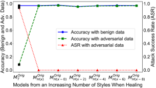
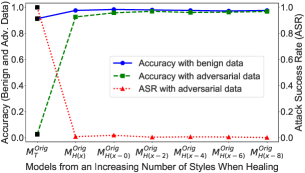
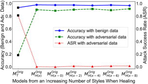
We investigate whether the performance of trojaned models (based on the three metrics described in Section V-A) improve as we increase the number of styles used in the healing process. We conduct our evaluation against BadNets, Trojaning (SQ), and Trojaning (WM) using the corresponding original testing sets. Figure 5 shows the results. For each of the attacks, we start with the corresponding trojaned model and proceed as follows. First, is evaluated with the original testing samples to measure the performance of the model before applying ( in -axis). The corresponding points in the plots are marked with a black square to highlight that these are the initial values of the metrics. Then, is taken through the healing process multiple times using incremental retraining sets to measure how the metrics vary as more styles are used (points to in -axis).
Figures 5a, 5b, and 5c show that the performance improves as is progressively applied. The three metrics tend to converge to the aimed values with just a few styles (considering the graphs of all the metrics, two styles suffice for all the cases). For the three attacks, the ASR drops to or close to 0.0%. Simultaneously, the accuracy with benign data converges to high values that outperform the initial accuracy of the trojaned model. This metric has percentage increases of 0.24%, 7.28%, and 3.63% in the best obtained healed models , , and for the attacks BadNets, Trojaning (SQ), and Trojaning (WM) respectively. For the accuracy with adversarial data, we also obtain a significant increase in these models. This accuracy increases 88.14%, 94.02%, and 72.66% in the models for the same order of attacks. An interesting behavior is observed in the case of Trojaning (WM). The accuracy with adversarial data significantly improves to values above 90% in all the cases, but always remains lower than the accuracy achieved with benign data. This phenomenon can be explained by the fact that the watermark overrides the object of interest (i.e., faces), covering certain key attributes of the faces (e.g., eyes, lips, etc.) used by models during the classification (a violation to the condition listed in Section III-B). As a consequence, some adversarial inputs with the watermark covering key attributes of the faces cannot be recognized to their true classes after applying because the resulting contents (face shapes plus watermark) are not part of the content of images present in the healing set . Note that a violation to condition means that attackers assume weak defenders who cannot perceive triggers even when they cover a significant portion of the input images (a less real-world feasible scenario from the standpoint of the attacker).
Findings. With a few styles (two in our case), reduces the ASR to or close to 0.00%, while ensures that both accuracies converge to close values equal or above the original accuracy when conditions - are satisfied.
VI-B Robustness When Processing Transformed Inputs
RQ2. How well do models learn to focus on content and how effective is when processing styled inputs?
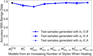
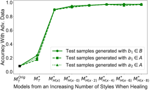
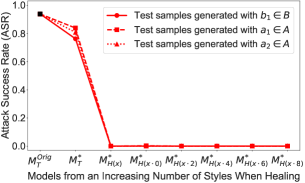
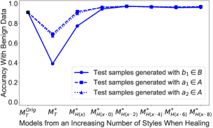
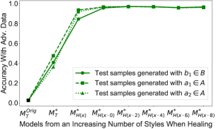
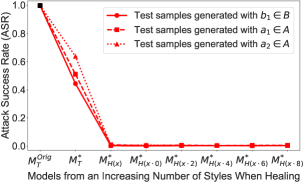
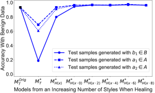
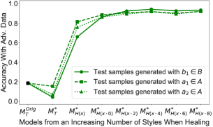
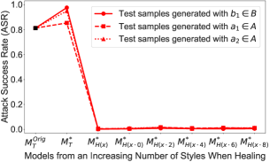
Following the methodology of the previous section, we now evaluate how well healed models learn to focus on the content of images, disregarding their styles. To this end, models are evaluated using three different styled or transformed versions of the testing set. One version is generated with the style base image , which is used in the healing process. The other two versions are obtained using the style base images and in , which are not used during the healing of the models. For each attack, we start again with the corresponding trojaned model evaluated with original samples to get the initial values of the metrics before applying ( in -axis). Following, is tested using transformed samples to measure the impact that the input transformation itself has on the performance ( in -axis). Finally, transformed samples are used to test the models healed through an incremental application of (points to in -axis).
Figure 6 shows the results. Each subfigure in it corresponds to one of the metrics and an attack. For all the metrics, the final performance of the healed models are nearly the same, regardless the styled version of the testing set used in the evaluation. The metrics tend to converge to sought values as more styles are used. This is a consequence of the increasing data augmentation achieved through the addition of new styles to the process. Both accuracies improve because the larger the retraining set is, the more samples with common content information the model receives. With the increasing sets, models are fine-tuned with enough samples for them to extract the contents of the training sample features, which are also present in the testing samples. Simultaneously, the attack success rate also drops because of this data augmentation. As the retraining set increases, models tend to forget the trigger because more parameter updates are executed in one epoch of training with samples not including the trigger. This is an expected behavior based on the findings of Liu et al. [12], who shows that this metric decreases as more benign data samples (original version only) are used to fine-tune DNN models.
Notice that the transformed testing datasets used in this evaluation are generated with both styles used and not used in the healing process. Hence, this experiment shows the effectiveness of on making models focus on content and not on styles during the classification. One interesting observation is that using styled images without healing the models does not prevent the attacks. The attacks become ineffective after applying with a few styles. Considering all the plots and metrics in Figure 6, four styles suffice.
After , the ASR is reduced to or close to 0.0%. In all the attacks, the accuracies with benign data (regardless the style) achieve high values that outperform the initial accuracies of the trojaned model. Using the best resulting healed models , and for the attacks BadNets, Trojaning (SQ), and Trojaning (WM) respectively, this metric grows 0.47%, 6.71%, and 3.2% when evaluated with the transformed testing set generated with . With respect to the accuracy with adversarial data, the metric increases 89.30%, 94.41%, and 75.65% with the same healed models.
Findings. With a few styles (four in our case), reduces the ASR to or close to 0.00%, while ensures both accuracies get values equal or above the original accuracy regardless the input style when conditions - hold.
VI-C Effect on Non-Trojaned Models
RQ3. What is the impact of on the accuracy (only benign data applies) of non-trojaned models?
One of the main challenges defending against trojan attacks is the lack of tools to determine whether a given model has a trojan. Due to this restriction, this section evaluates the impact has on the accuracy of an original non-trojaned model . Our goal is determining whether can be applied to any model (whether infected or not) without impairing its current performance (accuracy with benign data).
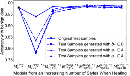
We take the non-trojaned version of the models created with the datasets GTSRB and VGG-Face through the healing process. Figure 7 shows the metric variation of the GTSRB model as styles are added to the healing process. Taking model tested with the transformed samples generated with as example, the accuracy improves from 97.91% to 98.37%. We get a similar graph (not included) with the VGG-Face model. In this case, the best performance is obtained with the model , with a percentage increase of 0.17%. These results prove that does not affect the accuracy of non-trojaned models. In contrast, the trends of the graphs shows that it at least remains the same if enough styles are used in the healing process.
Findings. can be equally applied to any model (either trojaned or not) as it does not impair its performance.
VI-D Healing Set Size and Number of Styles
RQ4. Does the number of styles required in the healing process depend on the size of the healing set ?
We investigate the relationship between the number of styles required to successfully apply and the size of the healing set. This is a key question because having access to extra training sets is challenging in real-world scenarios. As specified in Section V, previous experiments are run with healing sets of size 10% and 5% for the models infected with BandNets and Trojaning Attack respectively. We now replicate the same experiments progressively decreasing the size of these sets and selecting the model with the best performance in each case. Table IV shows that there is no relationship between size of the healing set and the number of styles needed to apply . This can be explained because the combination of some contents and styles add noise to the resulting retraining set, which make models to not monotonically improve as more styles are added. Whereby, defenders need to apply the best training practices to fine-tune the models with the generated data so as to obtain the best possible results.
Findings. There is no relationship between the size and the number of styles needed to successfully apply .
VI-E Performance and Comparison With the State-of-the-Art
RQ5. How well does perform compared to the state-of-the-art and what overhead it imposes at testing?
Table V shows the performance of and its comparison with the state-of-art Neural Cleanse [7]. To be complete in our comparison with fine-tuning-based methods, we also include a comparison with Retraining [12]. The table contains the accuracies (with both begin and adversarial data) and the ASR after applying the defensive methods. The first column specifies the attack used for the evaluation. DS refers to the size of the healing set. The initial values of the trojaned models (before applying any method) are included in Table VI.
In Table V, columns below ConFoc (Original Inputs) and ConFoc (Transformed Inputs) summarize the performance of our method using the best healed models (specified in Table IV) for different sizes of the healing set. As the names indicate, we tested with both original and transformed inputs. The other two techniques (Retraining and Neural Cleanse) were evaluated with original inputs as the methods require. With Retraining, we fine-tuned the model using the original healing set for multiple epochs and selected the best resulting model. In the case of Neural Cleanse, we proceeded exactly as indicated by the authors in [7]. We added the reversed-engineered triggers to 20% of the samples in the healing set and retrained the model for one epoch. The reversed-engineered triggers are provided by the authors in [55]. During the execution of this method, only the trigger related to Trojaning (WM) worked as expected. Whereby, we ran the Neural Cleanse method against BadNets and Trojaning (SQ) with the actual triggers used to conduct the attacks. This action does affect the performance of Neural Cleanse. In contrast, it represents the ideal scenario in which triggers are perfectly reverse-engineered and the produced corrected models provide the best possible results.
| Experimental Setup | Best Healed Model | ||
| Attack | DS | Model ID | No. Styles (Including Content) |
| BadNets | 10% | 7 | |
| Trojaning (SQ) | 5% | 3 | |
| Trojaning (WM) | 5% | 5 | |
| BadNets | 6.6% | 5 | |
| Trojaning (SQ) | 3.3% | 3 | |
| Trojaning (WM) | 3.3% | 2 | |
| BadNets | 3.3% | 5 | |
| Trojaning (SQ) | 1.67% | 2 | |
| Trojaning (WM) | 1.67% | 3 | |
| Experimental Setup | ConFoc (Original Inputs) | ConFoc (Transformed Inputs) | Retraining (Healing Set Only) | Neural Cleanse | |||||||||
| Attack | DS | Acc (Ben) | Acc (Adv) | ASR | Acc (Ben) | Acc (Adv) | ASR | Acc (Ben) | Acc (Adv) | ASR | Acc (Ben) | Acc (Adv) | ASR |
| BadNets | 10.0% | 97.21% | 96.51% | 0.00% | 97.44% | 97.67% | 0.00% | 96.98% | 96.51% | 0.00% | 97.21% | 65.35% | 0.00% |
| Trojaning (SQ) | 5.0% | 97.79% | 96.75% | 0.53% | 97.27% | 97.14% | 0.27% | 97.40% | 92.45% | 0.94% | 97.53% | 97.27% | 0.27% |
| Trojaning (WM) | 5.0% | 96.75% | 91.28% | 0.80% | 96.35% | 94.27% | 0.53% | 97.79% | 90.10% | 0.40% | 96.88% | 93.36% | 0.27% |
| BadNets | 6.66% | 97.21% | 96.98% | 0.00% | 97.21% | 97.21% | 0.00% | 96.28% | 94.42% | 0.00% | 97.21% | 54.42% | 0.00% |
| Trojaning (SQ) | 3.33% | 97.40% | 97.27% | 0.53% | 96.75% | 97.14% | 0.66% | 98.31% | 82.68% | 0.16% | 97.53% | 97.79% | 0.13% |
| Trojaning (WM) | 3.33% | 96.88% | 92.32% | 0.13% | 96.09% | 91.67% | 0.27% | 98.05% | 92.19% | 1.73% | 97.01% | 92.45% | 0.00% |
| BadNets | 3.33% | 96.05% | 96.05% | 0.00% | 97.21% | 97.21% | 0.00% | 95.12% | 96.05% | 0.00% | 97.21%, | 58.84% | 3.33% |
| Trojaning (SQ) | 1.67% | 98.05% | 96.09% | 0.67% | 96.35% | 96.88% | 0.27% | 98.05% | 82.94% | 0.16% | 96.61% | 96.09% | 0.00% |
| Trojaning (WM) | 1.67% | 97.27% | 91.15% | 0.13% | 95.96% | 92.84% | 0.27% | 97.66% | 83.72% | 9.08% | 96.48% | 89.58% | 1.34% |
| Attack | Acc (Ben) | Acc (Adv) | ASR |
| BadNets | 96.98% | 8.37% | 93.81% |
| Trojaning (SQ) | 91.15% | 2.73% | 99.73% |
| Trojaning (WM) | 93.36% | 18.62% | 81.18% |
As shown in the Table V, all the defensive methods produce high accuracy with benign data regardless the size of the healing set. In most cases, this metric is superior to the initial value of the trojaned model (see to Table VI). The main differences between the methods are observed in the accuracy with adversarial data (highlighted in light grey for all the methods) and the ASR. (with both original and transformed inputs) constantly gets high values in these two metrics, while the other methods produce values below 90% for the former and above 1% for the latter as the healing set decreases. These cases are marked in red in the table.
With respect to the accuracy with adversarial data, Retraining, as expected, tends to produce models with lower values in this metric as the healing sets become smaller in all the attacks [12]. Neural Cleanse produces models that perform well against both Trojaning Attacks and unwell against BadNets regardless the size of the healing set. This is because Neural Cleanse relies on updating the model parameters for one epoch only, which does not suffice to remove the learned trigger-related features. BadNets is conducted via poisoning, which means that the parameters of all model layers are adjusted during training. Whereby, to remove the effect of triggers, larger datasets or more epochs are required [12]. Trojaning Attack, in contrast, is a retraining technique that fine-tunes the last layers of the models (i.e., it changes less parameters) while inserting the trojan (see Section III-C). Hence, one epoch is enough to remove the trigger effect.
At this point, it is important to highlight that due to the violation of the condition as explained Section VI-A, produces models with lower values in the accuracy with adversarial data than those obtained with benign data in the case of Trojaning Attack (WM) (see dark grey cells in the table). These values, however are constantly above 90% and do not tend to decrease with the sizes of the healing set.
ConFoc Overhead. There is no clear advantage (with respect to the metrics) on using either original or transformed inputs with . However, there is a difference in the overhead caused at testing time. Transforming the inputs with Algoritm 3 directly imposes an 10-run average overhead of 3.14 s with 10 iterations of the optimizer LGBFS [52] over a Titan XP GPU. We reduce this runtime overhead to values around 0.015 s by applying the principles of Algorithm 1 and Algorithm 3 to train image transformation neural networks offline for each chosen style as proposed in [56]. This implementation is included in our prototype [16]. does not impose any overhead at testing if original inputs are used.
Findings. outperforms the state-of-the-art method regardless the size of the healing set, without imposing any overhead when original inputs are used in the evaluation.
VI-F Robustness Against Adaptive and Complex Triggers
RQ6. How effective is ConFoc protecting DNN models when adaptive and complex triggers are used?
This section evaluates against trojan attacks conducted with complex triggers. We conduct the attacks with BadNets because this approach extracts trigger-related features in all the layers of the model, making it more difficult to eliminate. The idea is to test of in the most complex scenarios. We make sure that the attacks comply with the conditions - specified in Section III-B. The complex triggers are described below using as reference the trigger (referred here to as original) and data split presented in Section V-B (see Figure 4). In the description, the sizes of the triggers correspond to a percentage of the larger side of the inputs.
-
•
Adaptive. We assume an adaptive attacker knowledgeable about who seek to mitigate the healing procedure by infecting the model with styled adversarial samples. The original trigger is added to the samples in the trojan set (trj). These samples are then transformed via using the base , which is used in the healing process enacting so the best scenario for the attacker. The target class is 19.
-
•
Larger. A white square of size is 15% (rather than the 10% size of original) located in the botton-right corner of the image. The target class is 19.
-
•
Random Pixel. A square of size 10% located in botton-right corner of the image, whose pixel values are randomly chosen. The target class is 19.
-
•
Multiple Marks. A trigger consisting of four marks: (1) the original white square in the botton-right corner, (2) the random pixel square described above located in the botton-left corner, (3) a white circle (circumscribed by a square of size 15%) located in top-left corner, and (4) the same circle but filled with random pixels located in the top-right corner. The target class is 19.
-
•
Many-to-One. Each of the multiple marks described above are added individually to the samples in the trojan set (trj). Namely, we create four trojan sets, each with one of the marks. The target class assigned to all the resulting adversarial samples in these sets is 19.
-
•
Many-to-Many. In this case we assign a different target class to each of trojan sets described above. The assignment is as follows: (1) botton-right mark targets class 19, (2) botton-left mark targets class 20, (3) top-right mark targets class 21, and (4) top-left mark targets class 22.
| Before ConFoc | After ConFoc | |||||
| Trigger | Acc (Ben) | Acc (Adv) | ASR | Acc (Ben) | Acc (Adv) | ASR |
| Adaptive | 98.14% | 2.33% | 100.0% | 98.14% | 97.91% | 0.00% |
| Larger | 97.67% | 2.56% | 99.76% | 97.67% | 97.91% | 0.00% |
| Random Pixel | 97.91% | 2.33% | 100.0% | 98.14% | 97.44% | 0.00% |
| Multiple Marks | 97.44% | 2.33% | 100.0% | 97.67% | 97.91% | 0.00% |
| Many-to-One | 96.51% | 20.93% | 80.48% | 97.44% | 97.21% | 0.00% |
| Many-to-Many | 97.91% | 21.63% | 80.00% | 97.91% | 98.14% | 0.00% |
Table VII shows the metric of the trojaned models before and after applying . Results show that effectively reduces the ASR to the minimum while ensures both accuracies remain close or better than the initial values.
Findings. effectively eliminate trojans on DNNs compromised with complex triggers, while ensures accuracy values that in average either equal or outperform the initial values of the model when conditions - are satisfied.
VII Conclusions and Future Work
We present a generic model hardening technique called to protect DNNs against trojan attacks. takes as input an infected model and produces a healed version of it. These models are healed by fine-tuning them with a small dataset of benign inputs augmented with styles extracted from a few random images. We run experiments on different models and datasets, infected with a variety of triggers by two different trojan attacks: BadNets and Trojaning Attack. Results show that increasingly reduces the sensitivity of trojaned models to triggers as more styles are used in the healing process. We proved that our method can be equally applied to any model (trojaned or not) since it does not impact the initial accuracy of the model. In comparison with the state-of-the-art, we validate that consistently correct infected models, regardless the dataset, architecture or attack variation. Our results leads us to new research questions related to the internal behavior of models. Future work will aim to investigate which neurons relate to the content of inputs. This information will be used to devise a novel white-box approach to detect misbehaviors based on the activation of these neurons.
References
- [1] T. Young, D. Hazarika, S. Poria, and E. Cambria, “Recent trends in deep learning based natural language processing,” ieee Computational intelligence magazine, vol. 13, no. 3, pp. 55–75, 2018.
- [2] A. Voulodimos, N. Doulamis, A. Doulamis, and E. Protopapadakis, “Deep learning for computer vision: A brief review,” Computational intelligence and neuroscience, vol. 2018, 2018.
- [3] S. Ren, K. He, R. Girshick, and J. Sun, “Faster r-cnn: Towards real-time object detection with region proposal networks,” in Advances in neural information processing systems, 2015, pp. 91–99.
- [4] B. Zhou, A. Lapedriza, J. Xiao, A. Torralba, and A. Oliva, “Learning deep features for scene recognition using places database,” in Advances in neural information processing systems, 2014, pp. 487–495.
- [5] O. M. Parkhi, A. Vedaldi, A. Zisserman et al., “Deep face recognition.” in bmvc, vol. 1, no. 3, 2015, p. 6.
- [6] P. Sermanet and Y. LeCun, “Traffic sign recognition with multi-scale convolutional networks.” in IJCNN, 2011, pp. 2809–2813.
- [7] B. Wang, Y. Yao, S. Shan, H. Li, B. Viswanath, H. Zheng, and B. Y. Zhao, “Neural cleanse: Identifying and mitigating backdoor attacks in neural networks,” in 2019 IEEE Symposium on Security and Privacy (SP). IEEE, 2019, p. 0.
- [8] G. Tao, S. Ma, Y. Liu, and X. Zhang, “Attacks meet interpretability: Attribute-steered detection of adversarial samples,” in Advances in Neural Information Processing Systems, 2018, pp. 7717–7728.
- [9] T. Gu, B. Dolan-Gavitt, and S. Garg, “Badnets: Identifying vulnerabilities in the machine learning model supply chain,” arXiv preprint arXiv:1708.06733, 2017.
- [10] X. Chen, C. Liu, B. Li, K. Lu, and D. Song, “Targeted backdoor attacks on deep learning systems using data poisoning,” arXiv preprint arXiv:1712.05526, 2017.
- [11] Y. Liu, S. Ma, Y. Aafer, W.-C. Lee, J. Zhai, W. Wang, and X. Zhang, “Trojaning attack on neural networks,” in 25nd Annual Network and Distributed System Security Symposium, NDSS 2018, San Diego, California, USA, February 18-221, 2018. The Internet Society, 2018.
- [12] Y. Liu, Y. Xie, and A. Srivastava, “Neural trojans,” in 2017 IEEE International Conference on Computer Design (ICCD). IEEE, 2017, pp. 45–48.
- [13] K. Liu, B. Dolan-Gavitt, and S. Garg, “Fine-pruning: Defending against backdooring attacks on deep neural networks,” in International Symposium on Research in Attacks, Intrusions, and Defenses (RAID). Springer, 2018, pp. 273–294.
- [14] S. Ma, Y. Liu, G. Tao, W.-C. Lee, and X. Zhang, “Nic: Detecting adversarial samples with neural network invariant checking,” in 26th Annual Network and Distributed System Security Symposium, NDSS, 2019, pp. 24–27.
- [15] L. A. Gatys, A. S. Ecker, and M. Bethge, “Image style transfer using convolutional neural networks,” in Proceedings of the IEEE conference on computer vision and pattern recognition, 2016, pp. 2414–2423.
- [16] M. Villarreal-Vasquez, ConFoc Repository, 2020. [Online]. Available: https://github.com/mvillarreal14/confoc
- [17] K. He, X. Zhang, S. Ren, and J. Sun, “Deep residual learning for image recognition,” in Proceedings of the IEEE conference on computer vision and pattern recognition, 2016, pp. 770–778.
- [18] J. S. J. Stallkamp, M. Schlipsing and C. Igel, “Man vs. computer: Benchmarking machine learning algorithms for traffic sign recognition,” Neural Networks, no. 0, pp. –, 2012.
- [19] O. M. Parkhi, A. Vedaldi, and A. Zisserman, “Deep face recognition,” in British Machine Vision Conference, 2015.
- [20] S. Zagoruyko and N. Komodakis, “Wide residual networks,” arXiv preprint arXiv:1605.07146, 2016.
- [21] A. Sharif Razavian, H. Azizpour, J. Sullivan, and S. Carlsson, “Cnn features off-the-shelf: an astounding baseline for recognition,” in Proceedings of the IEEE conference on computer vision and pattern recognition workshops, 2014, pp. 806–813.
- [22] J. Donahue, Y. Jia, O. Vinyals, J. Hoffman, N. Zhang, E. Tzeng, and T. Darrell, “Decaf: A deep convolutional activation feature for generic visual recognition,” in International conference on machine learning, 2014, pp. 647–655.
- [23] A. L. Maas, A. Y. Hannun, and A. Y. Ng, “Rectifier nonlinearities improve neural network acoustic models,” in Proc. icml, vol. 30, no. 1, 2013, p. 3.
- [24] B. Xu, N. Wang, T. Chen, and M. Li, “Empirical evaluation of rectified activations in convolutional network,” arXiv preprint arXiv:1505.00853, 2015.
- [25] Y. LeCun, L. Bottou, Y. Bengio, P. Haffner et al., “Gradient-based learning applied to document recognition,” Proceedings of the IEEE, vol. 86, no. 11, pp. 2278–2324, 1998.
- [26] N. Carlini and D. Wagner, “Towards evaluating the robustness of neural networks,” in 2017 IEEE Symposium on Security and Privacy (SP). IEEE, 2017, pp. 39–57.
- [27] I. J. Goodfellow, J. Shlens, and C. Szegedy, “Explaining and harnessing adversarial examples,” arXiv preprint arXiv:1412.6572, 2014.
- [28] A. Kurakin, I. Goodfellow, and S. Bengio, “Adversarial examples in the physical world,” arXiv preprint arXiv:1607.02533, 2016.
- [29] S.-M. Moosavi-Dezfooli, A. Fawzi, and P. Frossard, “Deepfool: a simple and accurate method to fool deep neural networks,” in Proceedings of the IEEE conference on computer vision and pattern recognition, 2016, pp. 2574–2582.
- [30] N. Papernot, P. McDaniel, S. Jha, M. Fredrikson, Z. B. Celik, and A. Swami, “The limitations of deep learning in adversarial settings,” in 2016 IEEE European Symposium on Security and Privacy (EuroS&P). IEEE, 2016, pp. 372–387.
- [31] K. Pei, Y. Cao, J. Yang, and S. Jana, “Deepxplore: Automated whitebox testing of deep learning systems,” in proceedings of the 26th Symposium on Operating Systems Principles. ACM, 2017, pp. 1–18.
- [32] T. B. Brown, D. Mané, A. Roy, M. Abadi, and J. Gilmer, “Adversarial patch,” arXiv preprint arXiv:1712.09665, 2017.
- [33] M. Sharif, S. Bhagavatula, L. Bauer, and M. K. Reiter, “Accessorize to a crime: Real and stealthy attacks on state-of-the-art face recognition,” in Proceedings of the 2016 ACM SIGSAC Conference on Computer and Communications Security. ACM, 2016, pp. 1528–1540.
- [34] N. Papernot, P. McDaniel, X. Wu, S. Jha, and A. Swami, “Distillation as a defense to adversarial perturbations against deep neural networks,” in 2016 IEEE Symposium on Security and Privacy (SP). IEEE, 2016, pp. 582–597.
- [35] W. Xu, D. Evans, and Y. Qi, “Feature squeezing: Detecting adversarial examples in deep neural networks,” arXiv preprint arXiv:1704.01155, 2017.
- [36] A. Madry, A. Makelov, L. Schmidt, D. Tsipras, and A. Vladu, “Towards deep learning models resistant to adversarial attacks,” arXiv preprint arXiv:1706.06083, 2017.
- [37] C. Szegedy, W. Zaremba, I. Sutskever, J. Bruna, D. Erhan, I. Goodfellow, and R. Fergus, “Intriguing properties of neural networks,” arXiv preprint arXiv:1312.6199, 2013.
- [38] S. Gu and L. Rigazio, “Towards deep neural network architectures robust to adversarial examples,” arXiv preprint arXiv:1412.5068, 2014.
- [39] A. N. Bhagoji, D. Cullina, C. Sitawarin, and P. Mittal, “Enhancing robustness of machine learning systems via data transformations,” in 2018 52nd Annual Conference on Information Sciences and Systems (CISS). IEEE, 2018, pp. 1–5.
- [40] D. Meng and H. Chen, “Magnet: a two-pronged defense against adversarial examples,” in Proceedings of the 2017 ACM SIGSAC Conference on Computer and Communications Security. ACM, 2017, pp. 135–147.
- [41] R. Shin and D. Song, “Jpeg-resistant adversarial images,” in NIPS 2017 Workshop on Machine Learning and Computer Security, vol. 1, 2017.
- [42] G. K. Dziugaite, Z. Ghahramani, and D. M. Roy, “A study of the effect of jpg compression on adversarial images,” arXiv preprint arXiv:1608.00853, 2016.
- [43] N. Das, M. Shanbhogue, S.-T. Chen, F. Hohman, L. Chen, M. E. Kounavis, and D. H. Chau, “Keeping the bad guys out: Protecting and vaccinating deep learning with jpeg compression,” arXiv preprint arXiv:1705.02900, 2017.
- [44] L. Deng, “The mnist database of handwritten digit images for machine learning research [best of the web],” IEEE Signal Processing Magazine, vol. 29, no. 6, pp. 141–142, 2012.
- [45] S. Ren, K. He, R. Girshick, and J. Sun, “Faster r-cnn: Towards real-time object detection with region proposal networks,” in Advances in neural information processing systems, 2015, pp. 91–99.
- [46] S. R. Safavian and D. Landgrebe, “A survey of decision tree classifier methodology,” IEEE transactions on systems, man, and cybernetics, vol. 21, no. 3, pp. 660–674, 1991.
- [47] I. Steinwart and A. Christmann, Support vector machines. Springer Science & Business Media, 2008.
- [48] K. Simonyan and A. Zisserman, “Very deep convolutional networks for large-scale image recognition,” arXiv preprint arXiv:1409.1556, 2014.
- [49] J. Deng, W. Dong, R. Socher, L.-J. Li, K. Li, and L. Fei-Fei, “ImageNet: A Large-Scale Hierarchical Image Database,” in CVPR09, 2009.
- [50] R. Arora, A. Basu, P. Mianjy, and A. Mukherjee, “Understanding deep neural networks with rectified linear units,” arXiv preprint arXiv:1611.01491, 2016.
- [51] J. Nagi, F. Ducatelle, G. A. Di Caro, D. Cireşan, U. Meier, A. Giusti, F. Nagi, J. Schmidhuber, and L. M. Gambardella, “Max-pooling convolutional neural networks for vision-based hand gesture recognition,” in 2011 IEEE International Conference on Signal and Image Processing Applications (ICSIPA). IEEE, 2011, pp. 342–347.
- [52] D. C. Liu and J. Nocedal, “On the limited memory bfgs method for large scale optimization,” Mathematical programming, vol. 45, no. 1-3, pp. 503–528, 1989.
- [53] R. A. Brualdi, H. J. Ryser et al., Combinatorial matrix theory. Springer, 1991, vol. 39.
- [54] G. Huang, M. Mattar, T. Berg, and E. Learned-Miller, “Labeled faces in the wild: A database for studying face recognition in unconstrained environments,” Tech. rep., 10 2008.
- [55] B. Wang, Neural Cleanse Repository, 2019. [Online]. Available: https://github.com/bolunwang/backdoor
- [56] J. Johnson, A. Alahi, and L. Fei-Fei, “Perceptual losses for real-time style transfer and super-resolution,” in European conference on computer vision. Springer, 2016, pp. 694–711.