Implications of a possible TeV break in the cosmic-ray electron and positron flux

Abstract

A TeV spectral break in the total flux of cosmic-ray electrons and positrons (CREs) at which the spectral power index softens from $\sim 3$ to $\sim 4$ has been observed by H.E.S.S. and recently confirmed by DAMPE with a high significance of $6.6~{}\sigma$. Such an observation is apparently inconsistent with the data from other experiments such as Fermi-LAT, AMS-02, and CALET. We perform a global analysis to the latest CRE data including Fermi-LAT, AMS-02, CALET, DAMPE, and H.E.S.S. with energy scale uncertainties taken into account to improve the consistency between the data sets. The fit result strongly favors the existence of the break at $\sim 1$ TeV with an even higher statistical significance of $13.3~{}\sigma$. In view of the tentative CRE break, we revisit a number of models of nearby sources, such as a single generic Pulsar Wind Nebula (PWN), known multiple PWNe from the ATNF catalog, and their combinations with either an additional Dark Matter (DM) component or a Supernova Remnant (SNR). We show that the CRE break at $\sim 1$ TeV, together with the known CR positron excess points towards the possibility that the nearby sources should be highly charge asymmetric. Among the models under consideration, the one with a PWN plus SNR is most favored by the current data. The favoured distance and age of the PWN and SNR sources are both within $0.6$ kpc and around $10^{5}$ yr respectively. Possible candidate sources include PSR J0954-5430, Vela and Monogem ring, etc. We find that for the models under consideration, the additional DM component is either unnecessary or predicts too much photons in tension with the H.E.S.S. data of $\gamma$-rays from the direction of the Galactic Center. We also show that the current measurement of the anisotropies in the arrival direction of the CRE can be useful in determining the properties of the sources.

I Introduction

High energy cosmic-ray electrons and positrons (CREs) lose their energies rapidly via inverse Compton scattering and synchrotron radiation during their propagation through the Galaxy. CREs with observed energy above TeV typically come from a distance within 1 kpc, which makes them an important probe of nearby sources. The existence of the nearby sources may contribute to spectral features in the CRE energy spectrum. Candidates of such CRE sources include: Pulsar Wind Nebulae (PWNe), Supernova Remnants (SNRs), and Dark Matter (DM) particle annihilation or decay, etc.

In recent years, with the successful running of several ground- and space-based experiments, the measurement of the CRE flux in the GeV–TeV region has been significantly improved. The CRE flux can be measured by ground-based imaging atmospheric Cherenkov telescopes such as H.E.S.S., VERITAS, and MAGIC. In 2009, the H.E.S.S. collaboration measured CRE flux in the energy range 340 GeV – 1.5 TeV, and found a spectral break at $\sim 0.9$ TeV with the power-law index softening from 3.0 to 4.1 (Aharonian:2009ah, ). The result was confirmed with higher statistics in the preliminary data of H.E.S.S. in 2018 (HESSICRC17, ). The VERITAS collaboration observed a similar break at a lower significance (Archer:2018chh, ). The results from MAGIC showed a trend of spectrum softening after $\sim$TeV, but is in overall agreement with a single power law in the energy range 100 GeV – 3 TeV, due to significant uncertainties (BorlaTridon:2011dk, ).

The satellite-borne Fermi-LAT experiment has measured the CRE spectrum up to 2 TeV (Abdollahi:2017nat, ). Although the Fermi-LAT data showed a trend of spectrum softening after around TeV, the whole CRE spectrum above 47 GeV can still be well described by a single power law with a power index $\sim 3.11$ due to significant energy reconstruction uncertainties. The AMS-02 experiment onboard the international space station (ISS) has measured the CRE spectrum up to 1 TeV (the CR electron flux reached 1.4 TeV recently (Aguilar:2019ksn, )), but did not observe any significant structure below TeV Aguilar:2019ksn . In 2017, the satellite-borne experiment DAMPE which has relatively large acceptance (compared with AMS-02) and high energy resolution (compared with Fermi-LAT) has released the first measurement on the CRE spectrum up to 4.6 TeV, which strongly favors a break at $\sim 0.9$ TeV at $6.6~{}\sigma$ significance. After the break, the CRE spectral power index softens from $\sim 3.1$ to $\sim 3.9$ (Ambrosi:2017wek, ). Recently, the CALET collaboration has extended the CRE measurement up to 4.8 TeV, and the result also supports a spectral softening at around 0.9 TeV (Adriani:2018ktz, ). The current CRE measurements from different experiments are apparently not in full agreement with each other in the energy range $\sim 30$ GeV – a few TeV. Increasing the statistics in the future is unlikely to resolve the problem as the current data below TeV are dominated by systematic uncertainties.

In this work, we perform a global analysis of the latest CRE data from Fermi-LAT, AMS-02, DAMPE, CALET, and H.E.S.S. We show that a consistent fit of all the five data sets can be achieved by including the uncertainties in the absolute energy scale of different experiments. This part of uncertainty is usually not added to the total uncertainties in the released data. The global fit result strongly favors the existence of a spectral break at around TeV. After the break, the CRE spectral power index softens from $\sim 3.10$ to $\sim 3.89$, which confirms the result of DAMPE at a higher significance $\sim 13.3~{}\sigma$.

In view of the tentative CRE break, we revisit a number of models of nearby sources, such as a single generic Pulsar Wind Nebula (PWN), known multiple PWNe from the ATNF catalog, and their combinations with either an additional dark matter (DM) component or a Supernova Remnant (SNR). In total six models are considered: A) a single PWN, B) all middle-aged PWNe from the ATNF catalog with a simplified assumption that they share a common spectral index and efficiency, C) a single PWN plus an additional DM component which annihilates directly into $2\mu$ final states, D) all middle-aged PWNe plus an additional DM component which annihilates directly into $2\mu$ final states, E) a single PWN plus a single SNR, F) middle-aged PWNe plus a single SNR and DM. The CRE break at $\sim\text{TeV}$, together with the CR positron spectrum peaking at $\sim 300$ GeV suggests the possibility that the nearby sources would be highly charge asymmetric. Consequently, we find that among these models, only models E and F can well account for the current CRE and CR positron spectra simultaneously. For model-E, the data favor a nearby middle-aged PWN with a spectral index $\sim 2$ and an energy cutoff at $\sim 0.8$ TeV. PSR J0954-5430 is a possible PWN candidate. The favored additional SNR turns out to have a spectral index $\sim 2.2$ and a total energy $\sim 5.5\times 10^{48}$ erg. Possible SNR candidates include Vela and Monogem ring. For model-F, the data favor a DM particle with mass $\sim$ 1 TeV and annihilation cross-section $\sim 1.69\times 10^{-24}~{}{\rm cm^{3}s^{-1}}$. The favored DM parameters are consistent with the limits derived from Fermi-LAT data of $\gamma$-rays from dwarf galaxies (Ackermann:2015zua, ), but still in tension with the H.E.S.S. data from the Galactic Center (GC) (Abdallah:2016ygi, ). In model-F, the middle-aged PWNe turn out to have a spectral $\sim 2$, and an efficiency $\sim 0.098$. The favored additional SNR for this model turns out to have a spectral index $\sim 1.9$ and a total energy $\sim 4.1\times 10^{48}$ erg. Possible SNR candidates include Vela and Monogem ring. In addition, we predict the dipole anisotropy in CRE flux for relevant models and compare them with the current upper-limits obtained by Fermi-LAT (Abdollahi:2017kyf, ). We find that the upper-limits on the CRE anisotropy could be a useful tool for understanding the properties of the $e^{\pm}$ sources in these models.

This paper is organized as follows: In Sec. II, we briefly overview the calculation of CR propagation and possible sources of CREs. In Sec. III, we perform a global analysis of the current CRE data. In Sec. IV, we discuss a number of models of nearby sources. In Sec. V, we summarize the conclusions of this work. The impact of the uncertainties in the propagation models on the conclusion is also discussed.

II PROPAGATION OF COSMIC RAYS IN THE GALAXY

II.1 The propagation model

The propagation of CR particles through the Galaxy can be approximated by a diffusion model in which the diffusion halo is parameterized by a cylinder with radius $R\simeq 20$ kpc and half-height $Z_{h}=1\sim 10$ kpc. The diffusion equation for the CR charged particles reads (Ginzburg:1990sk, ; Strong:2007nh, )

$$\frac{\partial\psi}{\partial t}=\nabla(D_{xx}\nabla\psi-\bm{V}_{c}\psi)+\frac{\partial}{\partial p}p^{2}D_{pp}\frac{\partial}{\partial p}\frac{1}{p^{2}}\psi-\frac{\partial}{\partial p}\left[\frac{\mathrm{d}p}{\mathrm{d}t}\psi-\frac{p}{3}(\nabla\cdot\bm{V}_{c})\psi\right]-\frac{1}{\tau_{f}}\psi-\frac{1}{\tau_{r}}\psi+Q(\bm{r},t,p),$$ (1)

where $\psi(\bm{r},t,p)$ is the CR number density per unit momentum, $D_{xx}$ is the spatial diffusion coefficient, and $\bm{V}_{c}$ is the convection velocity. The re-acceleration effect is described as diffusion in momentum space and is determined by the coefficient $D_{pp}$. The quantity $dp/dt$ stands for the momentum loss rate. $\tau_{f}$ and $\tau_{r}$ are the time scales for fragmentation and radioactive decay respectively. $Q(\bm{r},t,p)$ is the source term. The energy-dependent spatial diffusion coefficient $D_{xx}$ is parameterized as $D_{xx}=\beta D_{0}\left({\rho}/{\rho_{0}}\right)^{\delta}$, where $\rho=p/Ze$ is the rigidity of CR particles with electric charge $Ze$, $\delta$ is the spectral power index, $\rho_{0}$ is a reference rigidity, $D_{0}$ is a normalization constant, and $\beta=v/c$ is the velocity of CR particles. The momentum diffusion coefficient $D_{pp}$ is related to $D_{xx}$ as $D_{pp}D_{xx}=4V_{a}^{2}p^{2}/(3\delta(4-\delta^{2})(4-\delta))$, where $V_{a}$ is the Alfvèn velocity of disturbances in the hydrodynamical plasma (Ginzburg:1990sk, ). The source term of primary CR particles is expressed as $Q(\bm{r},t,p)=f(\bm{r},t)q(p)$, where $f(\bm{r},t)$ is the spatial distribution and $q(p)$ is the injection spectrum. The spatial distribution of the source is taken from Ref. (1996A&AS..120C.437C, ). The injection spectra of the primary nucleus are assumed to be a broken power law behavior, $q(p)\propto({\rho}/{\rho_{s}})^{\gamma_{\rm nucl}}$, with the injection index $\gamma_{\rm nucl}=\gamma_{\rm nucl,1}(\gamma_{\rm nucl,2})$ for the nucleus rigidity $\rho$ below (above) a reference rigidity $\rho_{s}$. The spatial boundary conditions are set by assuming that free particles escape beyond the halo, i.e., $\psi(R,z,p)=\psi(\bm{r},\pm Z_{h},p)=0$. The steady-state solution can be obtained by setting $\partial\psi/\partial t=0$.

In this work, we use the public code GALPROP-v54 (Strong:1998pw, ; MOSKALENKO:2001YA, ; STRONG:2001FU, ; MOSKALENKO:2002YX, ; PTUSKIN:2005AX, ) to numerically solve this equation for the CR propagation. The propagation parameters are fixed to the “MED” diffusion re-acceleration (DR) propagation model, which is obtained from a global fit to the proton and B/C data of AMS-02 using the GALPROP code (Jin:2014ica, ). Note that this model is different from the one proposed in Ref. (Donato:2003xg, ) which is based on semi-analytical solutions of the propagation equation. The main parameters of this model are summarized in Tab. 1. When CR particles propagate into the heliosphere, the flux of CR particles is affected by the solar wind and the heliospheric magnetic field. In order to account for the solar modulation, we adopt the force field approximation with a modulation potential $\phi=0.55$, which is consistent with the value adopted in deriving the “MED” model from the experimental data.

$R(\mbox{kpc})$	$Z_{h}(\mbox{kpc})$	$D_{0}$	$\rho_{0}$(GV)	$\delta$	$V_{a}(\mbox{km}/\mbox{s})$	$\rho_{s}$(GV)	$\gamma_{\rm nucl,1}/\gamma_{\rm nucl,2}$
20	3.2	6.50	4.0	0.29	44.8	10.0	1.79/2.45

TAB. 1: Values of the main parameters in the “MED” propagation model derived from fitting to the AMS-02 B/C and proton data based on the GALPROP code Jin:2014ica . The parameter $D_{0}$ is in units of $10^{28}~{}\mbox{cm}^{2}\cdot\mbox{s}^{-1}$.

II.2 Sources of primary and secondary CRE

SNRs in our Galaxy are often considered as the major source of primary CR particles. Charged particles can be accelerated to a very high energy by non-relativistic diffusive shock wave through the Fermi acceleration mechanism 1977DoSSR.234.1306K ; Blandford:1978ky ; Bell:1978zc ; Bell:1978fj . The supernova explosion rate in the Galaxy is $\sim 3$ per century. Thus the injection of the primary CR particles from the SNRs can be assumed to be a stable continuous source. The source term of the primary electrons from the SNRs can be written as

$$Q_{{\rm pri}}(\bm{r},t,p)=f(r,z)q_{{\rm pri}}(p),$$ (2)

where $f(r,z)$ is the spatial distribution and $q_{{\rm pri}}(p)$ is the injection spectrum of the source. The spatial distribution is assumed to follow the SNRs distribution (1996A&AS..120C.437C, )

$$f(r,z)=\left(\frac{r}{r_{\odot}}\right)^{a}\exp\left(-b\cdot\frac{r-r_{\odot}}{r_{\odot}}\right)\exp\left(-\frac{|z|}{z_{s}}\right),$$ (3)

where $r_{\odot}=8.5$ kpc is the distance from the Sun to the GC, $z_{s}\approx 0.2$ kpc is the characteristic height of the Galactic disk. The two parameters $a$ and $b$ are chosen to be $a=1.25$ and $b=3.56$, which are adopted to reproduce the Fermi-LAT $\gamma$-ray gradient (Trotta:2010mx, ; Tibaldo:2009spa, ). The typical injected spectra have the shape of a power-law with an exponential cut-off:

$$q_{{\rm pri}}(\rho)\propto\left(\frac{\rho}{1{\rm GV}}\right)^{-\gamma_{e}}\exp\left(-\frac{\rho}{\rho_{c}}\right),$$ (4)

where $\gamma_{e}$ is the power index, and $\rho_{c}$ is the exponential cutoff in rigidity.

During the propagation, the spallation process of the CR nuclei in the interstellar medium (ISM) will produce secondary particles. The corresponding source term is given by

$$Q_{{\rm sec}}(p)=\sum_{i=\mathrm{H,He}}n_{i}\sum_{j}\int c\beta_{j}n_{j}(p^{\prime})\frac{d\sigma_{ij}(p,p^{\prime})}{dp}dp^{\prime}$$ (5)

where $n_{i}$ is the number density of the interstellar gas, $n_{j}(p^{\prime})$ is the number density of CR particles, $d\sigma_{ij}(E,p^{\prime})/dE$ is the differential cross-section for the production of electrons and positrons from the interaction between CR particles and the interstellar gas. The production cross-sections can be obtained through parameterizations of the available pp-collision data Kamae:2006bf ; Tan:1984ha ; Badhwar:1977zf ; 1986ApJ…307…47D ; 1986A&A…157..223D , or using Monte-Carlo event generators with QCD inspired phenomenological models Huang:2006bp ; Sjostrand:2006za . The choice of different cross-section parameterizations can result in the change of the secondary electron/positron flux up to 30% Feng:2016loc ; Evoli:2017vim ; Lipari:2016vqk . The change in the cross-sections only leads to minor changes in the analysis, since the secondary electrons and positrons are subdominant in the high energy region. In this work, we employ the parameterization in 1986ApJ…307…47D ; 1986A&A…157..223D which is implemented in GALPROP-v54 Moskalenko:1997gh . As it can be seen from Eq. (5), for a given propagation model, the fluxes of the secondary CR electrons and positrons can be predicted from the distribution of primaries without free parameters.

In the GALPROP code, the primary electron source term is normalized in such a way that the flux of the primary electrons at a reference kinetic energy $E_{{\rm ref}}$ is reproduced. In this work, we fix the value of $E_{{\rm ref}}$ at $E_{{\rm ref}}=25$ GeV and fit the post-propagated normalization flux $N_{e}$ to the data.

II.3 CRE anisotropy

CREs at high energies are most probably from nearby sources, which may lead to visible anisotropy of CRE flux in the arrival direction. The measurement on CRE anisotropy can be a useful tool to constrain the properties of nearby CR source, which is complementary to the data of the total flux. In the diffusion model, the dipole anisotropy of CRE flux is given by

$$\Delta(E)=\frac{3D_{xx}(E)}{c}\frac{|\nabla\psi(E)|}{\psi(E)},$$ (6)

where $\psi(E)$ is the number density of CRE, and $c$ is the speed of light. For a collection of CRE sources, the total dipole anisotropy can be computed as (1971ApL…..9..169S, ):

$$\Delta\left(n_{\max},E\right)=\frac{1}{\psi_{\operatorname{tot}}(E)}\cdot\sum_{i}\frac{\mathbf{r}_{i}\cdot\mathbf{n}_{\max}}{\left\|\mathbf{r}_{i}\right\|}\cdot\psi_{i}(E)\Delta_{i}(E),$$ (7)

where $\psi_{i}(E)$ is the number density of CRE from each source $i$, $\mathbf{r}_{i}$ is the position of the source, $\Delta_{i}(E)$ is the dipole anisotropy from each source from Eq. (6), $\mathbf{n}_{\max}$ is the direction of maximum flux intensity, and $\psi_{\operatorname{tot}}(E)=\sum_{i}\psi_{i}(E)$ is the total CRE number density.

III a global analysis of the current CRE data

All the current measurements from different experiments show that the energy spectrum of CRE flux approximately follows a power law in a wide energy range, however, different experiments are apparently not in full agreement in details: $i)$ for energies below $\sim$ 140 GeV, the DAMPE data is slightly higher than that from all the other experiments. Starting from $\sim$ 70 GeV, the Fermi-LAT data of the CRE spectrum is harder than that measured by AMS-02 and CALET; $ii)$ for the energy range 140 GeV – 1 TeV, the data of Fermi-LAT and DAMPE is noticeably higher than that from AMS-02 and CALET while the H.E.S.S. data in this energy range is compatible with that from in AMS-02 and CALET; $iii)$ for energies above $\sim$ 1 TeV, the measured CRE spectra of DAMPE, CALET and H.E.S.S. all start to soften, while no significant spectral change was observed by Fermi-LAT in this energy region. Increasing the statistics in the future is unlikely to resolve the problem as the current data below TeV are dominated by systematic uncertainties. The absolute energy scale calibration is one of the key parts in the CRE flux measurements. The absolute energy scale is defined as $S\equiv E/E_{t}$, where $E_{t}$ and $E$ are the true and measured energies respectively. The measured flux $\Phi(E)$ is related to the true flux $\Phi_{t}(E_{t})$ by $\Phi(E)=\Phi_{t}\left(E_{t}\right)/S$. The value of $S$ and its relative uncertainty $\delta_{s}=\Delta S/S$ can be determined by using the geomagnetic cutoff at around 10 GeV. The released experimental data usually include the corrections for the absolute energy scale $S$, while the uncertainties in $S$ (i.e. $\delta_{s}$) are not included. The consistency between the current CRE data can be improved by considering the uncertainties in the absolute energy scale. A full treatment of energy scale uncertainty in each experiment is complicated. In this work, we adopt a naive method of the error propagation in which the systematic uncertainty on the CR flux due to the energy scale uncertainty is estimated by

$$\Delta\Phi/\Phi\approx\left|\frac{E}{\Phi(E)}\frac{d\Phi}{dE}+1\right|\delta_{s},$$ (8)

For a signal power-law spectrum with a spectral index $\gamma$, the above expression can be simplified to $\Delta\Phi/\Phi\approx|\gamma-1|\delta_{s}$, which is in agreement with the literature (Ackermann:2010ij, ). The details of the estimation of $\Phi(E)$, $d\Phi/dE$ and $\Delta\Phi/\Phi$ for each experimental data set are given in Appendix A.

The values of the energy scale uncertainty for each experiment are summarized below:

• AMS-02 (both CRE and CR positron measurement), the typical value of $\delta_{s}$ is $\sim 4\%$ at 0.5 GeV, $\sim 2\%$ from 2 GeV to 300 GeV, and $\sim 2.6\%$ at 1.4 TeV (Aguilar:2019ksn, ; Aguilar:2019owu, ; Kounine:2017pss, );

• Fermi-LAT, $2\%$ for the whole energy range (Abdollahi:2017nat, );

• DAMPE, the current preliminary value is $1.26\%$ in the whole energy range (DAMPEISM19, );

• CALET, the energy scale is determined by two independent methods, geomagnetic cutoff and MIP calibrations (Adriani:2017efm, ; Adriani:2018ktz, ). The corresponding values are $1.035\pm 0.009~{}(\text{stat})$ and $1.000\pm 0.013~{}(\mathrm{sys})$, respectively. The reason for such a difference is yet to be understood. Since the released CALET data already include the correction of the absolute energy scale $S$ (not the uncertainty $\delta_{s}$) using the value from the geomagnetic cutoff (Adriani:2018ktz, ), we take the corresponding uncertainty to be $\delta_{s}=0.009$.

• H.E.S.S. the value is $15\%$ which is much larger than that from the space-based experiments (Aharonian:2009ah, ).

	$\Phi_{0}$	$\gamma_{1}$	$\gamma_{2}$	$\gamma_{3}$	$E_{\mathrm{br1}}$	$E_{\mathrm{br2}}$	$\bm{\chi^{2}/\mathrm{d.o.f.}}$
FERMI$\dagger$	5.39 $\pm$ 0.05	3.25 $\pm$ 0.02	3.06 $\pm$ 0.01	3.27 $\pm$ 0.13	49.7 $\pm$ 3.4	847.7 $\pm$ 293.8	$\bm{2.8/31}$
DAMPE	5.42 $\pm$ 0.05	3.20 $\pm$ 0.08	3.09 $\pm$ 0.01	4.01 $\pm$ 0.18	45.9 $\pm$ 16.5	925.2 $\pm$ 92.4	$\bm{25.6/32}$
CALET	4.57 $\pm$ 0.05	-	3.15 $\pm$ 0.01	3.83 $\pm$ 0.33	-	959.5 $\pm$ 225.5	$\bm{13.6/29}$
AMS-02	4.68 $\pm$ 0.03	3.24 $\pm$ 0.02	3.13 $\pm$ 0.00	-	45.4 $\pm$ 4.3	-	$\bm{9.4/31}$
H.E.S.S.	4.04 $\pm$ 0.12	-	3.02 $\pm$ 0.07	3.67 $\pm$ 0.02	-	804.8 $\pm$ 78.5	$\bm{0.2/14}$
Global Fit	5.00 $\pm$ 0.05	3.23 $\pm$ 0.03	3.10 $\pm$ 0.01	3.86 $\pm$ 0.16	52.6 $\pm$ 7.6	975.9 $\pm$ 131.3	$\bm{302.3/155}$
Global Fit*	5.02 $\pm$ 0.05	3.24 $\pm$ 0.07	3.10 $\pm$ 0.01	3.89 $\pm$ 0.14	46.0 $\pm$ 11.2	987.8 $\pm$ 110.2	$\bm{170.5/155}$

• the LAT energy reconstruction uncertainties are considered.

• the absolute energy scale uncertainties are considered.

TAB. 2: The fit parameters corresponding to the fit of Eq. (9) to the CRE data with energies above 25 GeV from Fermi-LAT Abdollahi:2017nat , DAMPE Ambrosi:2017wek , CALET Adriani:2018ktz , AMS-02 Aguilar:2019ksn , H.E.S.S. HESSICRC17 and to the CRE data from all the five experiments with and without including the energy scale uncertainties. The reduced $\chi^{2}$ of each fit is also listed. $\Phi_{0}$ is in units of $10^{-6}~{}\mathrm{m}^{-2}\mathrm{sr}^{-1}\mathrm{s}^{-1}\mathrm{GeV}^{-1}$, $E_{\mathrm{br1}}$ and $E_{\mathrm{br2}}$ are in units of $\mathrm{GeV}$.

We perform a global fit to the CRE flux data with a smoothly broken power-law (Ackermann:2013wqa, ; Ambrosi:2017wek, )

$$\Phi_{\mathrm{CRE}}(E)=\Phi_{0}\left[1+\left(\frac{E_{\mathrm{br1}}}{E}\right)^{k}\right]^{(\gamma_{1}-\gamma_{2})/k}\left(\frac{E}{300\mathrm{GeV}}\right)^{-\gamma_{2}}\left[1+\left(\frac{E}{E_{\mathrm{br2}}}\right)^{k}\right]^{-(\gamma_{3}-\gamma_{2})/k},$$ (9)

where $\Phi_{0}$ is a normalization factor, $E_{\mathrm{br1,br2}}$ are the break energies and $\gamma_{1,2,3}$ are the spectral power indexes. The smoothness parameter is fixed to $k=10$. Other parameters are determined through maximizing the log likelihood (or minimizing the $\chi^{2}$ function)

$$-2\ln\mathcal{L}=\chi^{2}=\sum_{i}\frac{\left(\Phi_{i}-\Phi_{\exp,i}\right)^{2}}{\sigma_{\exp,i}^{2}},$$ (10)

where $\Phi_{i}$ is the theoretical value, $\Phi_{\exp,i}$ and $\sigma_{\exp,i}$ are the measured value and uncertainty of the CRE flux. We consider the data in the energy range 25 GeV $\sim$ 15 TeV. For the Fermi-LAT CRE data, the energy reconstruction uncertainty is included. The low energy break $E_{\mathrm{br1}}$ is not used for the fit to the CALET data, as it can not be constrained by the CALET data for energies above 25 GeV.

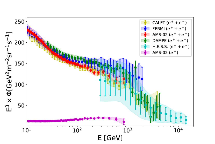
We first fit to the CRE data of each experiment independently, and then make a global fit to the data from all the five experiments with and without including the energy scale uncertainties. The best-fit parameters and the goodness-of-fit are summarized in Tab. 2.

From Tab. 2, one can see that without including the energy scale uncertainty the global fit leads to $\chi^{2}/\mathrm{d.o.f.}\approx 302.3/155$. After including this part of uncertainty, the fit result gives $\chi^{2}/\mathrm{d.o.f.}\approx 170.5/155$, which is a significant improvement of the goodness-of-fit. Thus the consistency between the data sets is improved after including the energy scale uncertainty. In Fig. 1, we show the best-fit CRE flux from the global fit together with its 95% C.L. uncertainty band.

FIG. 1: CRE flux from a global fit to the latest CRE data from all five experiments (Fermi-LAT Abdollahi:2017nat , DAMPE Ambrosi:2017wek , CALET Adriani:2018ktz , AMS-02 Aguilar:2019ksn , and H.E.S.S. HESSICRC17 ) with including the energy scale uncertainties. The purple band corresponds to the parameters varying within 95% C.L. The error bars represent the total uncertainties (quadratic sum of the statistical and systematic uncertainties) with the energy scale uncertainties included.

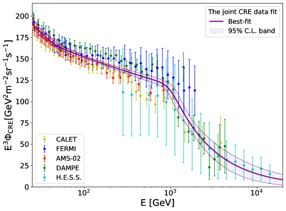
The individual fits to each experiment show that most current measurements (expect for AMS-02) favor the existence of a spectral break at around TeV at some extent. To quantify the significance of the spectral break, we adopt a test statistic of $\text{TS}=-2\ln(\mathcal{L}_{0}/\mathcal{L})$, where $\mathcal{L}(\mathcal{L}_{0})$ stands for the likelihood with (without) the break. We find that even the Fermi-LAT data slightly favor a high energy spectral break $E_{\mathrm{br2}}$ at $847.7\pm 293.8$ GeV with $\chi^{2}/\mathrm{d.o.f.}=2.8/31$. Another fit without the energy break $E_{\mathrm{br2}}$, results in $\chi^{2}/\mathrm{d.o.f.}=3.6/33$. Thus roughly corresponding to a significance of $\sim 0.43~{}\sigma$ for a $\chi^{2}$-distribution with two degrees of freedom, which is consistent with the conclusion of the Fermi-LAT collaboration, i.e., not observing significant structures in the high energy range.

The significance of the high energy spectral break in the global fit is estimated as follows: We perform global fits in the energy range of 55 GeV – 15 TeV for two models. One is a single power-law model $\Phi=\Phi_{0}(E/300~{}\mathrm{GeV})^{-\gamma}$ and the other one is a smoothly broken power-law model $\Phi=\Phi_{0}(E/300~{}\mathrm{GeV})^{-\gamma_{1}}[1+(E/E_{\mathrm{b}})^{k}]^{-(\gamma_{2}-\gamma_{1})/k}$ with $k=10$. The single power-law fit gives $\gamma=3.16\pm 0.01$, with $\chi^{2}/\mathrm{d.o.f.}=338.8/122$. The smoothly broken power-law fit gives $\gamma_{1}=3.10\pm 0.01$, $\gamma_{2}=3.89\pm 0.16$, $E_{\mathrm{b}}=988\pm 120$, and $\chi^{2}/\mathrm{d.o.f.}=157.0/120$. Compared to the single power-law model, the $\chi^{2}$ value is reduced by 181.8 for two less degrees of freedom. From the TS value we estimate the significance of the spectral break is $\sim 13.3~{}\sigma$. The significance from the global fit is even higher than that from the DAMPE data alone, which is easy to understand as the other experiments (except for AMS-02) also favor the existence of the spectral break.

IV Theoretical Models and Results

The TeV break in the CRE flux, if confirmed, may constitute another CR lepton anomaly complementary to the well-known CR positron excess. The break may originate from extra sources or non-standard mechanisms of CR acceleration and propagation. In this work, we shall focus on the first probability. Possible nearby extra sources include PWNe, SNRs and DM annihilation or decay, etc. We investigate what kind of sources or combination of sources can account for both the CRE break and the CR positron excess.

IV.1 Charge-symmetric electron–positron sources

We first consider charge-symmetric sources which produce equal amount of CR electrons and positrons with the same energy spectrum. PWNe and DM annihilation are among such kind of sources.

PWNe are well-known powerful sources of primary electrons and positrons which are believed to be produced in the magnetosphere and accelerated by the termination shock. The time-evolution of the luminosity of the associated pulsar can be written as $\dot{\xi}=\dot{\xi}_{0}\left(1+t/\tau_{0}\right)^{-\frac{n+1}{n-1}}$, where $\dot{\xi}_{0}$ is the initial spin-down luminosity, $t$ is the age of the pulsar, $\tau_{0}$ is the luminosity decay time, and $n$ is the breaking index Gaensler:2006ua . This expression can be derived from a largely model-independent assumption where the pulsar spin-down is described by $\dot{\Omega}=-K\Omega^{n}$, where $\Omega$ is the rotation frequency and $K$ is a global constant. If $t/\tau_{0}\gg 1$, the luminosity drops rapidly and can be considered as a burst-like source of energy release. In the opposite limit where $t/\tau_{0}\ll 1$, the luminosity can be approximated as a constant in time.

In this work, we shall simply model the emission of electrons/positrons from PWNe as a burst-like process, as commonly adopted in the literature Hooper:2008kg ; Yin:2013vaa ; Wang:2017hsu ; Malyshev:2009tw ; Grasso:2009ma ; Delahaye:2010ji ; DiBernardo:2010is ; DiMauro:2014iia ; Manconi:2016byt ; DiMauro:2017jpu ; Manconi:2018azw . In the burst-like scenario, the source term of a PWN at origin and $t=0$ is assumed to have a power-law energy spectrum with an exponential cutoff

$$Q(E,\bm{r},t)=Q_{0}\left(\frac{E}{{\rm GeV}}\right)^{-\gamma}\exp\left(-\frac{E}{E_{c}}\right)\delta(\bm{r})\delta(t),$$ (11)

where $\gamma$ is the spectral power index and $E_{c}$ is the cutoff energy. The normalization factor $Q_{0}$ is related to the total injected energy $E_{\mathrm{tot}}$ by

$$E_{\mathrm{tot}}=\int_{E_{\text{min}}}^{\infty}EQ(E,\bm{r},t)dEd\bm{r}dt$$ (12)

where the integration lower limit is set to $E_{\text{min}}=0.1$ GeV. For PWNe the total injection energy is assumed to be a fraction $\eta$ of the total spin-down energy $W_{0}$ of the associated pulsar, namely $E_{\text{tot}}=\eta W_{0}$. In the magnetic-dipole (MD) emission model the value of $W_{0}$ is given by $W_{0}=\dot{\mathcal{E}}t(1+t/{\tau_{0}})$, where $t$ and $\dot{\mathcal{E}}$ are the age and the spin-down luminosity of the pulsar, respectively. The typical luminosity decay time $\tau_{0}$ is taken to be $10$ kyr Aharonian:1995zz , which is commonly adopted in the literature (see e.g. Hooper:2017gtd ; Yin:2013vaa ; Wang:2017hsu ; DiMauro:2014iia ; Manconi:2016byt ). Note that a constant emission of electrons from PWN is also possible and has been extensively discussed. For instance, in a recent analysis Fornieri:2019ddi the authors approximated pulsar age $t$ with its characteristic age $t_{\rm ch}=P/2\dot{P}$, and calculated the luminosity decay time using the MD model in which $\tau_{0}^{\mathrm{MD}}=3Ic^{3}/B_{p}^{2}R^{6}\Omega_{0}^{2}$, where $I$ is the moment of inertia, $B_{p}$ is the polar surface magnetic field, and $\Omega_{0}$ is the initial frequency. They estimated the ratio $t_{\rm ch}/\tau_{0}^{\rm MD}$ for the nearby pulsars in the ATNF catalog and found that the typical values of $t/\tau_{0}$ are lower than unity ($\sim 0.3$), which points towards a constant energy injection. Note, however, that so far a reliable estimation of the initial period ($P_{0}=2\pi/\Omega_{0}$) is only available for a very limited number of pulsars 2004hpa..book…..L ; FaucherGiguere:2005ny , which requires independent estimation of the true age $t$ of the related pulsar (e.g. the pulsar may have a historical association of a known supernova explosion to determine its true age $t$), and precise measurement of the pulsar braking index. We have estimated the ratio $t/\tau_{0}^{\rm MD}$ for the pulsars which have proper estimation of $\Omega_{0}$ summarized in Table 7 of FaucherGiguere:2005ny , and find that the values are in a wide range $\sim 0.1-2.1$, which suggests that the characteristic of luminosity evolution with time for different pulsars could be different. Note also that the pulsars associated with constant-luminosity injection are typically young with ages around a few thousand years. The ones with older ages are more likely to be associated with the burst-like injection. For more detailed discussions on the electron/positron emission time scale in PWNe, we refer to Fornieri:2019ddi and references therein.

For high energy CR electrons/positrons, the propagation can be simplified by neglecting convection and re-acceleration as they are only important at low energies. Thus only the energy-dependent diffusion and the energy loss due to synchrotron and Inverse Compton scatterings are relevant. The energy-dependent spatial diffusion coefficient is assumed to be $D(E)\simeq D_{0}\left({E}/4{\rm GeV}\right)^{\delta}$. The energy-loss rate is parameterized as ${\mathrm{d}E}/{\mathrm{d}t}=-b_{0}E^{2}$ with $b_{0}=1.4\times 10^{-16}~{}{\rm GeV^{-1}s^{-1}}$ Grasso:2009ma . For nearby sources, one can adopt a spherically symmetric boundary condition such that the Green’s function of the propagation equation for the burst-like source in Eq. (11) can be obtained analytically (Atoian:1995ux, )

$$\psi(E,t,\bm{r})=\frac{Q_{0}}{\pi^{3/2}r_{{\rm diff}}^{3}}\left(1-\frac{E}{E_{{\rm max}}}\right)^{\gamma-2}\left(\frac{E}{{\rm GeV}}\right)^{-\gamma}\exp\left(-\frac{E}{(1-E/E_{{\rm max}})E_{{\rm c}}}\right)\exp\left(-\frac{r^{2}}{r_{{\rm diff}}^{2}}\right),$$ (13)

where $E_{{\rm max}}=(b_{0}t)^{-1}$ is the maximum energy of electron/positron after propagation. The diffusion length $r_{{\rm diff}}$ is given by $r_{\mathrm{diff}}(E,t)\approx 2\sqrt{\lambda(E)D(E)t}$, where $\lambda(E)=[1-(1-E/E_{\mathrm{max}})^{1-\delta}]/[(1-\delta)E/E_{\mathrm{max}}]$.

Electrons and positrons can also be produced via halo DM annihilation or decay. In this work, we shall focus on the DM annihilation as it is essential for all the thermal relic models, and the extension of the analysis from DM annihilation to DM decay is straightforward. DM particles in the Galactic halo may annihilate into the standard model particles and make extra contributions to the CR electron and positron fluxes. The source term of primary electrons and positrons from the annihilation of Majorana DM particles takes the following form

$$Q_{{\rm DM}}(\bm{r},p)=\frac{\rho(\bm{r})^{2}}{2m_{\chi}^{2}}\langle\sigma v\rangle\sum_{X}\eta_{X}\frac{dN^{(X)}}{dp},$$ (14)

where $\rho(\bm{r})$ is the DM energy density profile, $m_{\chi}$ stands for the DM particle mass, $\langle\sigma v\rangle$ is the velocity-weighted annihilation cross section, $dN^{(X)}/dp$ is the injection energy spectrum from DM particles annihilating into electrons and positrons via all possible intermediate states $X$ and $\eta_{X}$ is the corresponding branching fraction. The fluxes of CR electrons and positrons from DM annihilation depend mildly on the choice of DM halo profile. In this work, we adopt the Einasto profile (Einasto:2009zd, )

$$\rho(\bm{r})=\rho_{\odot}\exp\left[-\left(\frac{2}{\alpha_{E}}\right)\left(\frac{r^{\alpha_{E}}-r_{\odot}^{\alpha_{E}}}{r_{s}^{\alpha_{E}}}\right)\right],$$ (15)

with $\alpha_{E}\approx 0.17$ and $r_{s}\approx 20$ kpc. The local DM energy density is taken to be $\rho_{\odot}=0.43\text{ GeV}\text{ cm}^{-3}$ (Salucci:2010qr, ). In this work, the injection spectra $dN^{(X)}/dp$ from DM annihilation are calculated using the numerical package PYTHIA 8 Sjostrand:2007gs .

It is known that DM annihilation as the dominant contribution to the CR positron excess is severely constrained. The lack of excess in the CR antiproton flux excludes the DM annihilation directly into $q\overline{q}$, $W^{+}W^{-}$ and $Z^{0}Z^{0}$ final states. The $e^{+}e^{-}$ channel leads to a very sharp spectral structure which cannot fit the observed positron flux. The leptonic channel $\tau^{+}\tau^{-}$ channel is also ruled out by the Fermi-LAT data on the $\gamma$-rays from the dwarf spheroidal galaxies (dSphs) (Ackermann:2015zua, ). Only the $\mu^{+}\mu^{-}$ channel is marginally compatible with the positron data. Note that the bump structure of the positron spectrum predicted from the $\mu^{+}\mu^{-}$ annihilation is relatively narrow compared with the broad excess observed by AMS-02. In this work, we shall only consider DM as a subdominant component of the nearby sources, with the normalization as a free parameter to be determined by the data.

As for the astrophysical explanations for the CR positron excess, two kinds of PWN explanations have been proposed and extensively discussed. The one is considering a single nearby PWN as the major source of high energy $e^{\pm}$ Hooper:2017gtd ; Yuksel:2008rf ; Pato:2010im ; Hooper:2008kg ; Yin:2013vaa ; Wang:2017hsu . The other one is considering the contributions from all known PWNe and usually assuming a common spectral index Malyshev:2009tw ; Grasso:2009ma ; Delahaye:2010ji ; DiBernardo:2010is ; DiMauro:2014iia ; Manconi:2016byt ; DiMauro:2017jpu ; Manconi:2018azw . In view of the possible TeV CRE break, we revisit these two kinds of PWN hypotheses and their combination with a DM component with $\mu^{+}\mu^{-}$ final states.

• Model-A (single PWN) We assume a generic nearby PWN with the age $T_{\mathrm{psr}}$, distance $d_{\mathrm{psr}}$, spectral index $\gamma_{\mathrm{psr}}$, cut-off energy $E_{c,\mathrm{psr}}$, efficiency $\eta_{\mathrm{psr}}$ and spin-down luminosity $\dot{\mathcal{E}}_{\mathrm{psr}}$ of the associated pulsar determined through fitting to data. Since the parameter $\eta_{\mathrm{psr}}$ and $\dot{\mathcal{E}}_{\mathrm{psr}}$ are degenerate in the expression of $E_{\mathrm{tot,psr}}$, we take the product $\eta_{\mathrm{psr}}\dot{\mathcal{E}}_{\mathrm{psr}}$ as a single parameter. Thus there are five free parameters {$T_{\mathrm{psr}}$, $d_{\mathrm{psr}}$, $\gamma_{\mathrm{psr}}$, $E_{c,\mathrm{psr}}$, $\eta_{\mathrm{psr}}\dot{\mathcal{E}}_{\mathrm{psr}}$} in this model.

• Model-B (Multiple PWNe) We consider the middle-aged PWNe with observed age $t_{{\rm obs}}$ in the range 50 kyr $<t_{{\rm obs}}<$ $10^{4}$ kyr from the most updated ATNF catalog (Manchester:2004bp, ). We simply assume a common spectral index $\gamma$, efficiency $\eta$, and exponential cutoff $E_{c}$ for all PWNe. Thus there are three free parameters {$\gamma$, $\eta$, $E_{c}$} in this model.

• Model-C (single PWN + DM) This model consists of all the primary and secondary astrophysical contributions as that in Model-A plus the $e^{\pm}$ fluxes produced by DM with a typical $2\mu$ annihilation channel. The DM particle mass $m_{\chi}$ and cross section $\langle\sigma v\rangle$ are allowed to vary freely in the global fit. Thus compared with Model-A, this model has two more free parameters.

• Model-D (multiple PWNe + DM) This model consists of all the primary and secondary astrophysical contributions as that in Model-B plus the $e^{\pm}$ fluxes produced by DM with a typical $2\mu$ annihilation channel. The DM particle mass $m_{\chi}$ and cross section $\langle\sigma v\rangle$ are allowed to vary freely in the global fit. Thus compared with Model-B, this model has two more free parameters.

For the primary and secondary CRE background components, three additional free parameters {$\gamma_{e}$, $\rho_{c}$, $N_{e}$} are introduced. We adopt the “MED” propagation model and fit the parameters of the primary electron spectrum. We consider the CRE data from the five experiments (Fermi-LAT Abdollahi:2017nat , AMS-02 Aguilar:2019ksn , DAMPE Ambrosi:2017wek , CALET Adriani:2018ktz , and H.E.S.S. HESSICRC17 ) and the CR positron data from AMS-02 Aguilar:2019owu with energy scale uncertainty included. Only the data with energies above 25 GeV will be included in the fits to reduce the influence of the solar modulation. In total 196 data points are included in the analyses. We perform a Bayesian analysis to the data. To efficiently explore the high-dimensional parameter space of the models, we adopt the MultiNest sampling algorithm Feroz:2007kg ; Feroz:2008xx ; Feroz:2013hea . Details of the Bayesian statistical framework can be found in Appendix B.

FIG. 2: CRE (left) and CR positron (right) fluxes for the best-fit parameters of the charge-symmetric models (Model A, B, C, and D) described in Sec. IV.1. The black dotted, blue dashed, blue dash-dotted, and red dashed curves represent the contribution from the background, the single PWN, the middle-aged PWNe and the DM with a typical $2\mu$ annihilation channel respectively. The black solid curve represents the sum of all the components in each plot. The best-fit CRE flux and the 95% C.L. uncertainty band (green curve and band) from a global fit to the latest CRE data with a smoothly broken power-law model are also illustrated for comparison.

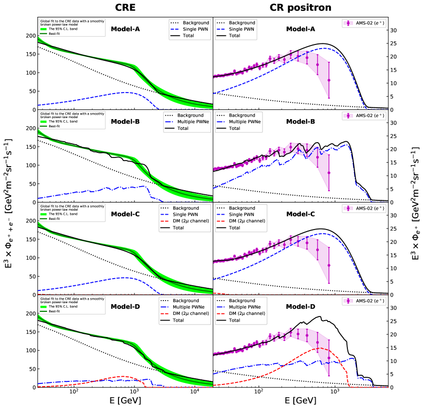
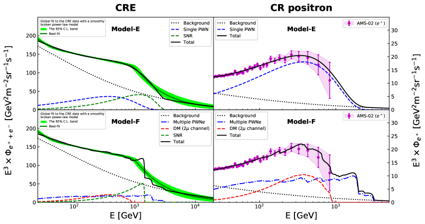
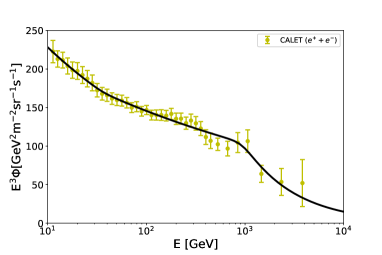
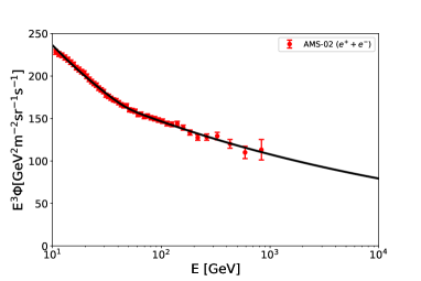
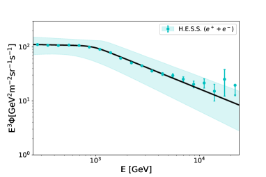
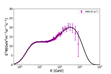
The results of the fit are presented in Fig. 2. As the figure shows, the TeV break measured in the CRE spectrum can be well reproduced by Model-A, -C and -D, but difficult for Model-B. For Model-C, the fit result shows that the nearby PWN as a dominant source is favored. The contribution from DM annihilation is quite small. Compared with Model-A, this model does not show any improvement in the goodness-of-fit as the Bayes factor is around 1.2. Therefore, the additional DM component in this model is unnecessary. For Model-D, the fit result shows that the additional DM component can significantly improve the agreement with the data. Compared to Model-B, the Bayes factor for Model-D is greater than 150, and the minimum $\chi^{2}$ value is reduced by 45.6 for two less degrees of freedom.

Although some models (Model-A and -D) could give a successful fit with a $\chi^{2}/\mathrm{d.o.f.}\sim 1.1-1.2$, we find that in general none of the models from A to D can well reproduce the CR positron flux measured by AMS-02. This is related to the difference in the energy regions where the CRE and CR positron spectra start to soften. The steepening of the measured CRE spectra appears at around TeV, while the dropoff of the measured positron spectrum appears at around 300 GeV. The different behavior of the CRE and CR positron spectra makes the models based on charge-symmetric $e^{\pm}$ sources in difficulty.

IV.2 Charge-asymmetric electron–positron sources

In view of the difficulties in charge-symmetric source models, it seems that to simultaneously account for both the CRE and CR positron flux data, extra charge-asymmetric $e^{\pm}$ sources are needed. SNR is a known source to contribute dominantly primary CR electrons only. Whereas, the details of the release mechanism of electrons from SNRs are poorly known and still under debate Blasi:2013rva ; Caprioli:2009fv ; Ohira:2011xq ; Gabici:2009ak ; Blasi:2011fi ; Fornieri:2020xai . In this work, we adopt a simplified model, the burst-like injection model. The calculation of CR electrons from SNR is mostly the same as that of PWN. The models based on a more realistic emission mechanism that electrons escape from SNR when its energy is larger than the maximal energy of electrons that can be confined in SNR have been extensively studied Ohira:2011xq ; Blasi:2011fi ; Gabici:2009ak ; Caprioli:2009fv . In these models, the escape of electrons from SNR takes place in such a way that higher energy electrons escape earlier in the evolution, while lower energy ones leave later. The analysis in Gabici:2009ak shows that the high energy electrons are emitted within a few thousand years from the supernova explosion. This timescale is much smaller than the age of sources typically considered to explain the CRE data at Earth, which supports the burst-like emission is a good approximation in our analysis.

In this section, we add a SNR component to the models previously considered. We shall focus on the extension of Model-A and Model-D as these two models fit the CRE data better than other models.

• Model-E (single PWN + SNR) This model consists of all the primary and secondary astrophysical contributions as that in Model-A plus the electron flux produced by a nearby SNR. The age $T_{\mathrm{snr}}$, distance $d_{\mathrm{snr}}$, spectral index $\gamma_{\mathrm{snr}}$, cut-off energy $E_{c,\mathrm{snr}}$, and the total energy emitted into electrons $E_{\mathrm{tot,snr}}$ of the SNR are determined through fitting to data. Thus compared with Model-A, this model has five more free parameters.

• Model-F (multiple PWNe + DM + SNR) This model consists of all the astrophysical and DM contributions as that in Model-D plus the electron flux produced by a nearby SNR. The age $T_{\mathrm{snr}}$, distance $d_{\mathrm{snr}}$, spectral index $\gamma_{\mathrm{snr}}$, cut-off energy $E_{c,\mathrm{snr}}$, and the total energy emitted into electrons $E_{\mathrm{tot,snr}}$ of the SNR are determined through fitting to data. Thus compared with Model-D, this model has five more free parameters.

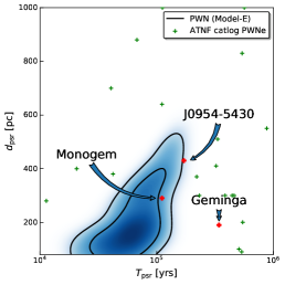
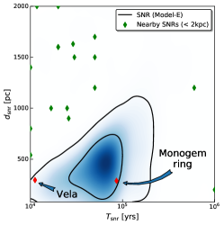
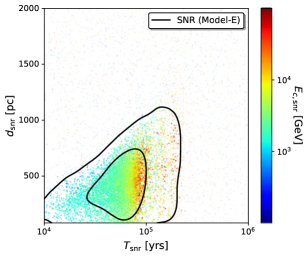
For Model-E, the fit result shows that the additional SNR can significantly improve the agreement with the data. Compared with Model-A, the Bayes factor for this model is $\sim 81$, and the minimum $\chi^{2}$ value is reduced by 23.9 for five less degrees of freedom. The additional SNR for this model turns out to be $\sim$ 57 kyr old, located at $\sim$ 0.5 kpc from the Earth, with a spectral index $\sim$ 2.2, an exponential cutoff energy $\sim$ 4.1 TeV, and a total energy $\sim 5.5\times 10^{48}$ erg. Compared to the PWN in this model, the additional SNR mainly contributes its electrons at around TeV. In the middle panel of Fig. 3, we plot the allowed regions for the SNR in the ($T_{\mathrm{snr}}$, $d_{\mathrm{snr}}$) plane at $68\%$ and $95\%$ C.L., together with the nearby known SNRs ($<2~{}\mathrm{kpc}$) summarized in Table C.1. of (Delahaye:2010ji, ). There are two SNRs, Vela and Monogem ring, falling in the regions allowed by the data. From the right panel of Fig. 3, it can be seen that the SNRs falling in the allowed regions come in two kinds: one has an injection cutoff $E_{c,\mathrm{snr}}$ around several TeV, the other is sufficient old ($T_{\mathrm{snr}}\geq 10^{5}~{}{\rm{yrs}}$) which suffers from a cooling cutoff $E_{\mathrm{max,snr}}$ around TeV. Both ensure that the electron spectrum produced by the additional SNR drops sharply around TeV. The cutoff energy for the PWN in Model-E is found to be $\sim 0.8$ TeV, smaller than the one in Model-A ($\sim 3.2$ TeV), while the spectral index $\gamma_{\mathrm{psr}}$ and the product $\eta_{\mathrm{psr}}\dot{\mathcal{E}}_{\mathrm{psr}}$ are similar to Model-A. In Model-E, less electron-positron pairs are produced by the PWN in high energy region, which results in a good agreement to the CR positron spectrum. The corresponding reduction in the CRE spectrum is offset by the electrons produced by the SNR. In the left panel of Fig. 3, we plot the allowed regions for the PWN in the ($T_{\mathrm{psr}}$, $d_{\mathrm{psr}}$) plane at $68\%$ and $95\%$ C.L. As the figure shows, the Monogem pulsar falls in the regions allowed by the data, PSR J0954-5430 is on the edge of the regions and could be a possible candidate once the uncertainty on the determination of the distance and age of the pulsar is taken into account.

FIG. 3: Results for Model-E described in Sec. IV.2. Left panel shows the allowed regions at 68% and 95% C.L. in ($T_{\mathrm{psr}}$, $d_{\mathrm{psr}}$) plane for the PWN in this model, comparing with the PWNe listed in the ATNF catalog. Middle and Right panels show the allowed regions 68% and 95% C.L. in ($T_{\mathrm{snr}}$, $d_{\mathrm{snr}}$) plane for the SNR in this model. The nearby known SNRs (¡ 2 kpc) are illustrated in the middle panel for comparison. The scatter points in the right panel represent the posterior samples and are colored by the values of the cutoff energy of the SNR.

The Monogem pulsar is widely considered to be a possible origin of the CR positron excess (see e.g.(Hooper:2008kg, ; Hooper:2017gtd, ; Yuksel:2008rf, ; Yin:2013vaa, )). However, the recent measurement of the surface brightness profile of TeV nebulae surrounding Monogem by HAWC (Abeysekara:2017old, ) suggests that the diffusion coefficient within a few tens of pc of these this pulsar is significantly lower than that expected in the ISM. The HAWC collaboration claimed that such a low diffusion coefficient led to a negligible positron flux at Earth, disfavoring it as the source of the observed CR positron excess. In some two-zone diffusion models, the low diffusion region is only restricted to a small region close to the pulsar, and a larger diffusion coefficient is possible outside the TeV nebula, thus Monogem remains to be the best candidate (Hooper:2017tkg, ; Fang:2018qco, ; Profumo:2018fmz, ). However, it was recently argued that after considering the GeV $\gamma$-ray observation of the nebula surrounding Monogem provided by Fermi-LAT, Monogem was still disfavored (Shao-Qiang:2018zla, ; DiMauro:2019yvh, ).

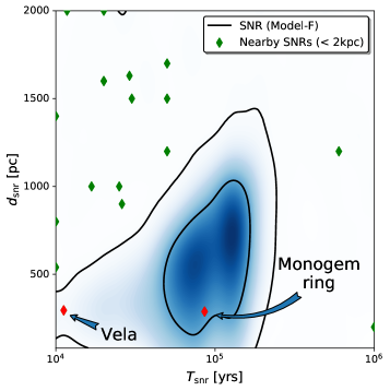
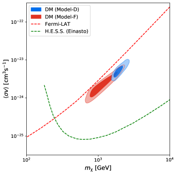
For Model-F, the additional SNR can also significantly improve the agreement with the data. Compared with Model-D, the Bayes factor for this model is $\sim 22$, and the minimum $\chi^{2}$ value is reduced by 25.4 for five less degrees of freedom. The additional SNR for this model turns out to be $\sim$ 152 kyr old, located at $\sim$ 0.54 kpc from the Earth, with a spectral index $\sim$ 1.9, and a total energy $\sim 4.1\times 10^{48}$ erg. The maximum energy of electrons surviving from cooling process for the SNR is $\sim 1.47$ TeV. Compared to the multiple PWNe and the DM component in this model, the additional SNR mainly contributes its electrons at around TeV. In Fig. 4, we plot the allowed regions for the SNR in the ($T_{\mathrm{snr}}$, $d_{\mathrm{snr}}$) plane at $68\%$ and $95\%$ C.L, together with the nearby known SNRs ($<2~{}\mathrm{kpc}$) summarized in Table C.1. of (Delahaye:2010ji, ). There are two SNRs, Vela and Monogem ring, falling in the regions allowed by the data. The DM particle in this model turns out to be with mass $\sim$ 1 TeV and cross section $\sim 1.69\times 10^{-24}~{}{\rm cm^{3}s^{-1}}$, which is less massive than that in Model-D ($\sim$ 1.9 TeV), while the favored parameters for the middle-aged PWNe are similar to Model-D. In Model-F, less electron-positron pairs are produced by the DM in high energy region, which resulting in a good agreement to the CR positron spectrum. The corresponding reduction in the CRE spectrum is offset by the electrons produced by the additional SNR. In Fig. 5, we plot the allowed regions at 68% and 95% C.L. in ($T_{\mathrm{psr}}$, $d_{\mathrm{psr}}$) plane for the DM of both Model-D and -F. As the figure shows, the allowed regions are consistent with the limits derived from Fermi-LAT data of $\gamma$-rays from dwarf galaxies, but in tension with the H.E.S.S. data from the GC. It is necessary to note that the constraints derived from the GC observation suffer from large uncertainty of the DM density around the GC. For instance, for a cored DM density with a core radius of 500 pc, the limits are one order of magnitude weaker (HESS:2015cda, ), while changing the DM density around the GC will not significantly affect the fit to the CRE and CR positron data. The constraints derived from the dwarf galaxies are not sensitive to the choice of the DM profile.

FIG. 4: The allowed regions at 68% and 95% C.L. in ($T_{\mathrm{psr}}$, $d_{\mathrm{psr}}$) plane for the SNR in Model-F, comparing with the known SNRs within 2 kpc.

FIG. 5: The allowed regions at $68\%$ and $95\%$ C.L. in ($m_{\chi}$, $\langle\sigma v\rangle$) plane for the DM in Model-D (blue contours) and in Model-F (red contours). The $95\%$ C.L. upper-limits given by Fermi-LAT Ackermann:2015zua (red dashed curve) and H.E.S.S. Abdallah:2016ygi (green dashed curve) are also plotted for comparison.

For both Model-E and -F, the fit results show that a large total injection energy $\log_{10}(E_{\rm tot}/{\rm erg})=48.0\pm 0.7$ of the additional SNR is favored by data. For a standard Supernova (SN) explosion event that carries $O(10^{51})$ erg of kinetic energy, this corresponds to a conversion efficiency into electrons about $\log_{10}f=-3.0\pm 0.7$, which is consistent with the limits given in the literature Delahaye:2010ji within uncertainties.

We have also considered other possibilities such as the combination of multiple PWNe plus a SNR. We find that the inclusion of the additional SNR can significantly improve the agreement with the CRE data, but have no visible effect on the prediction of CR positron flux. The predicted positron spectrum in this model is similar to that of Model-B (multiple PWNe), thus can not well explain the data either. The additional SNR for this model turns out to be favored with age $\sim$ 12 kyr old, located at $\sim$ 0.19 kpc from the Earth, a spectral index $\sim$ 1.7, a cutoff energy $\sim 492$ GeV, and a total injection energy $\sim 1.1\times 10^{47}$ erg. Compared to the multiple PWNe components in this model, the additional SNR mainly contributes its electrons at around several hundred GeV. Since this model can not well reproduce the CR positron flux measured by AMS-02, We will not discuss it further.

FIG. 6: Same as Fig. 2, but for the charge-asymmetric models (Model-E and -F) described in Sec. IV.2. The contribution from the additional SNR is represented by the green-dashed curve.

FIG. 7: Left panel illustrates the allowed regions for the position of the SNR in Model-E, which are derived by comparing the predicted CRE dipole anisotropy from the best fit to the CRE and the CR positron data with the upper-limits given by Fermi-LAT Abdollahi:2017kyf . The PWN in this model is assumed to be in the position with Galactic coordinate, $\left(0^{\circ},0^{\circ}\right)$, $\left(180^{\circ},0^{\circ}\right)$, $\left(0^{\circ},+90^{\circ}\right)$ and $\left(0^{\circ},-90^{\circ}\right)$ respectively. Right panel illustrates the predictions for the dipole anisotropy of the total CRE flux within the 95% C.L. uncertainty band derived from fitting to the CRE and the CR positron data for Model-F. The SNR in this model is assumed to be in the position with Galactic coordinate, $\left(0^{\circ},0^{\circ}\right)$, $\left(180^{\circ},0^{\circ}\right)$, $\left(0^{\circ},+90^{\circ}\right)$ and $\left(0^{\circ},-90^{\circ}\right)$ respectively. The 95% C.L. upper-limits given by Fermi-LAT Abdollahi:2017kyf are also plotted for comparison.

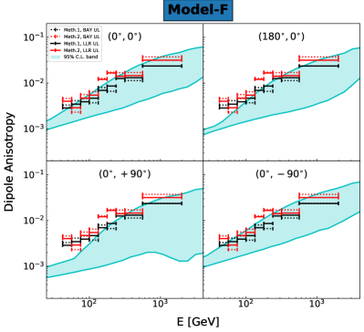
In addition, we compute the dipole anisotropy of CRE flux predicted by Model-E and -F by using the method described in Eq. (7) and then compare the results with the existing upper limits from Fermi-LAT Abdollahi:2017kyf . The anisotropies from the CRE background component and the DM component are computed by Eq. (6) with the GALPROP code. The anisotropy from discrete PWN/SNR sources is given

$$\Delta_{s}(E)=\frac{3}{2c\lambda(E)}\frac{|\bm{r}|}{t},$$ (16)

which is obtained from Eq. (13). The term $\lambda(E)$ is insensitive to the value of $\delta$. Varying the value of $\delta$ from 0.3 to 0.5 for a typical $10^{5}$ year PWN/SNR, the uncertainty in $\lambda(E)$ is found to be within 5%.

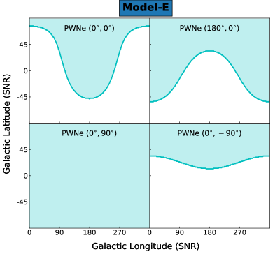
For Model-E, it is no simple task to give the total CRE anisotropy as the positions of the PWN and the SNR in this model are arbitrary. To have a clear view of how this model is constrained by the current CRE anisotropy observations, we pick up four representative positions with Galactic coordinate, $\left(0^{\circ},0^{\circ}\right)$, $\left(180^{\circ},0^{\circ}\right)$, $\left(0^{\circ},+90^{\circ}\right)$ and $\left(0^{\circ},-90^{\circ}\right)$ for the PWN and scan the position of the SNR. We compute the predicted CRE anisotropy (averaged over the energy bins given by Fermi-LAT Abdollahi:2017kyf ) for the best-fit parameters listed in Tab. 13. We compare our predictions to the Fermi-LAT upper-limits on the CRE anisotropy, choosing the more constraining results named Bayesian Method 1 in Abdollahi:2017kyf . Whenever our predictions overestimate one data point, we consider the position pair for the PWN and the SNR as excluded. In the left panel of Fig. 7, we illustrate the position pairs surviving from the Fermi-LAT limits. As the figure shows, the CRE anisotropy observations could indeed provide a valuable information on the positions of the PWN and SNR.

For Model-F, only the position of the SNR is arbitrary. Here, we pick up four representative positions with Galactic coordinate, $\left(0^{\circ},0^{\circ}\right)$, $\left(180^{\circ},0^{\circ}\right)$, $\left(0^{\circ},+90^{\circ}\right)$ and $\left(0^{\circ},-90^{\circ}\right)$ for the SNR and compute the CRE anisotropy for all the configurations within 95% C.L. selected by fitting to the CRE and CR positron spectra. In the right panel of Fig. 7, we illustrate our anisotropy predictions, together with the upper-limits given by Fermi-LAT. As the figure shows, our predictions reach the limits given by Fermi-LAT. Thus, the dipole anisotropy in the CRE arrival direction could set additional constraints to this model.

The predicted CRE anisotropies of both Model-E and -F reach the current Fermi-LAT limits and some parameter spaces are excluded. The future Chinese Space Station based instrument HERD is expected to have a better capability of anisotropy detection than Fermi-LAT due to a better energy resolution for electrons and a better electron/proton separation power Zhang:2014qga . It is planned for operation starting around 2025 for about 10 years and may provide insights into these two models.

V discussions/conclusions

In this work, we have employed the “MED” model as a benchmark model, in which the power-law index in the diffuse coefficient is $\delta\approx 0.3$. The value of $\delta$ in the “MED” model is very close to 1/3 from the Kolmogorov diffusion 1991RSPSA.434….9K . Moreover, the latest AMS-02 B/C data at high rigidities is well described by a single power with index $\Delta=0.333\pm 0.014(\mathrm{fit})\pm 0.005(\mathrm{syst})$, which is in good agreement with the Kolmogorov diffusion. The value of $\delta$ depends on the analysis framework, e.g. the recent analysis based on a semi-analytical approach yields $\delta\approx 0.43-0.53$ Genolini:2019ewc , the analyses based on the numerical code DRAGON and GALPROP yield a value of 0.45 Fornieri:2019ddi and 0.36 Xue:2019esp , respectively.

For an estimation of the uncertainties in CR propagation model, we consider three representative propagation models, the “MIN”, “MED”, and “MAX” models in Jin:2014ica . These models correspond to typical change due to the height of the propagation halo. We have checked that varying the main propagation parameters in the allowed ranges found in Jin:2014ica the electron/positron fluxes are included between the fluxes obtained for the “MIN” and “MAX” propagation models. The choice of different propagation models can result in the change of the secondary electron/positron flux up to 25%, but has no significant effect on the primary electron flux. For the total CRE background components, including both the primary and secondary electrons/positrons, the change of the flux is only within a few percent levels. The change in the propagation models only leads to minor changes in our analysis, since the secondary electrons and positrons are subdominant in the high energy region. For the DM-induced electrons/positrons, we checked the “MIN”, “MED”, and “MAX” models and found that the uncertainty in the positron/electron flux from DM annihilation into $2\mu$ is within a factor of 1.5. Rescaling the favored DM parameter spaces found in Model-F with the “MED” model (see in Fig. 5) by multiplying $\langle\sigma v\rangle$ by a factor of 1.5, most parameter spaces are still under the upper-limits given by Fermi-LAT. In this work, the propagation of the electrons/positrons from discrete PWN/SNR is calculated by an analytical approach with a spherically symmetric infinite boundary condition, and the fluxes of that are related to the propagation parameters $D_{0}$ and $\delta$ through the diffusion length $r_{\rm{diff}}$ (see in Eq. (13)). Changing the propagation model from “MED” to “MIN” (“MAX”) model can lead to a rescaling of $r_{\rm{diff}}$ by a factor of 0.74 (1.28). To reproduce the CRE and CR positron data, the favored distance $d_{\rm psr(snr)}$ and total energy that emitted into electrons and positrons $E_{\rm tot,psr(snr)}$ of the PWN/SNR are expected to be rescaled by a factor of 0.74 (1.28) and 0.41 (2.1), respectively.

The CRE anisotropy in the arrival direction mainly comes from nearby sources (PWN/SNR), which mainly depends on the age and distance of the source (see in Eq. (16)). As mentioned above, the change in the propagation models can lead to the change of source distance by about 27%, thus a similar amount of change is expected in the CRE anisotropy.

In this paper, we have performed a global analysis to the latest CRE data including Fermi-LAT, AMS-02, CALET, DAMPE, and H.E.S.S. We showed that a consistent fit of all the five data sets can be achieved by including the absolute energy scale uncertainties of each experiment. The global fit result strongly favors the existence of a break at $\sim 1$ TeV. After the break, the CRE spectral power index softens from $\sim 3.10$ to $\sim 3.89$, which confirms the result of DAMPE at a higher significance $\sim 13.3~{}\sigma$.

In view of the tentative CRE break, we have revisited a number of models of nearby sources, such as a single generic PWN, known multiple PWNe from the ATNF catalog, and their combinations with either an additional DM component or a SNR. We showed that the CRE break at $\sim 1$ TeV, together with the CR positron spectrum peaking at $\sim 300$ GeV points towards the possibility that the nearby sources are highly charge asymmetric. Among the models under consideration, only the model with a PWN plus SNR (labeled Model-E in our paper) and the model with all middle-aged PWNe plus a SNR and a DM component which annihilates directly into $2\mu$ (labeled Model-F in our paper), can well account for the current CRE and CR positron spectra simultaneously. For Model-E, the data favor a nearby middle-aged PWN with a spectral index $\sim 2$ and an energy cutoff at $\sim 0.8$ TeV. Possible PWN candidates include Monogem and PSR J0954-5430, while Monogem is excluded by the observation of HAWC. The favored additional SNR turns out to have a spectral index $\sim 2.2$ and a total energy $\sim 5.5\times 10^{48}$ erg. Possible SNR candidates include Vela and Monogem ring. For Model-F, the data favor a DM particle with mass $\sim$ 1 TeV and annihilation cross-section $\sim 1.69\times 10^{-24}~{}{\rm cm^{3}s^{-1}}$. The favored parameters are consistent with the limits derived from Fermi-LAT data of $\gamma$-rays from dwarf galaxies, but in tension with the H.E.S.S. data from the GC. The middle-aged PWNe in this model turn out to have a spectral $\sim 2$, and an efficiency $\sim 0.098$. The favored additional SNR for this model turns out to have a spectral index $\sim 1.9$ and a total energy $\sim 4.1\times 10^{48}$ erg. Possible SNR candidates include Vela and Monogem ring. In addition, we calculated the predicted dipole anisotropy on CRE flux for both models and compared it with the present upper-limits given by Fermi-LAT. We showed that the present Fermi-LAT data on the CRE anisotropy could be useful in understanding the properties of the $e^{\pm}$ sources in our models.

In the near future, with increased statistics and improved understanding of the detector’s performance, more consistent measurements of CRE flux among different experiments might be achieved, which will provide remarkable insights into the models tested in the present analysis.

VI Acknowledgment

This work is supported in part by the National Key R&D Program of China No. 2017YFA0402204 and by the National Natural Science Foundation of China (NSFC) No. 11825506, No. 11821505, No. U1738209, No. 11851303 and No. 11947302.

Appendix A Systematic uncertainty on the flux due to the energy scale uncertainty

To evaluate the systematic uncertainties on the fluxes of CRE and CR positron due to the energy scale uncertainties with Eq. (8), one needs to know the flux $\Phi(E)$ and its derivative $\Phi^{\prime}(E)$ first. In this work, the flux $\Phi(E)$ is approximated by a smooth curve with parameters determined through fitting to the flux data. The derivative $\Phi^{\prime}(E)$ can then be obtained straightforwardly from $\Phi(E)$. The CRE data from Fermi-LAT Abdollahi:2017nat , DAMPE Ambrosi:2017wek , CALET Adriani:2018ktz , and AMS-02 Aguilar:2019ksn are fitted with a smoothly broken power-law curve given by Eq. (9). The data with energy above 10 GeV are considered. The best-fit parameters and the goodness-of-fit of each individual fit are summarized in Tab. 3. From Tab. 3, one can see that the smoothly broken power-law model is a good approximation to the measured spectrum as the $\chi^{2}/\mathrm{d.o.f.}$ of each individual fit is less than 1. For the CRE data of H.E.S.S. HESSICRC17 , we adopt the parameterization reported in the International Cosmic Ray Conference HESSICRC17 :

$$E^{3}\frac{\mathrm{d}N}{\mathrm{d}E}=N_{0}\left(\frac{E}{(1\mathrm{TeV})}\right)^{3-\Gamma_{1}}\left(1+\left(\frac{E}{E_{b}}\right)^{\frac{1}{\alpha}}\right)^{-\left(\Gamma_{2}-\Gamma_{1}\right)\alpha}.$$ (17)

Tab. 4 lists the best-fit parameters from HESSICRC17 , which are obtained through fitting to the H.E.S.S. CRE data. The latest CR positron data from AMS-02 is well described by the minimal model Aguilar:2013qda ; Accardo:2014lma ; Cavasonza:2016qem ; Aguilar:2019owu , in which the positron flux is parametrized as the sum of a diffuse term and a source term

$$\Phi_{e^{+}}(E)=\frac{E^{2}}{\hat{E}^{2}}\left[C_{d}\left(\hat{E}/E_{1}\right)^{\gamma_{d}}+C_{s}\left(\hat{E}/E_{2}\right)^{\gamma_{s}}\exp\left(-\hat{E}/E_{s}\right)\right],$$ (18)

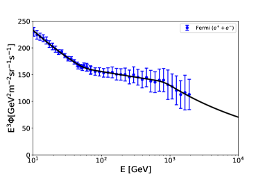
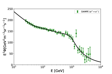
where $\hat{E}=E+\phi_{e^{+}}$ is the energy of particles in the interstellar space and $\phi_{e^{+}}$ is the effective solar potential. Tab. 5 lists the best-fit parameters from Aguilar:2019owu , which are obtained by fitting to the latest AMS-02 positron data with the minimal model. In Fig. 8, we illustrate the comparisons of the best-fitting curves and the measured spectra for all the experimental data described above.

CRE	$\Phi_{0}$	$\gamma_{1}$	$\gamma_{2}$	$\gamma_{3}$	$E_{\mathrm{br1}}$	$E_{\mathrm{br2}}$	$\bm{\chi^{2}/\mathrm{d.o.f.}}$
FERMI$\dagger$	5.40 $\pm$ 0.05	3.21 $\pm$ 0.00	3.06 $\pm$ 0.01	3.27 $\pm$ 0.13	56.1 $\pm$ 3.4	822.6 $\pm$ 274.7	$\bm{3.7/40}$
DAMPE	5.42 $\pm$ 0.05	3.20 $\pm$ 0.08	3.09 $\pm$ 0.01	4.01 $\pm$ 0.18	45.9 $\pm$ 16.5	925.2 $\pm$ 92.4	$\bm{25.6/32}$
CALET	4.59 $\pm$ 0.05	3.23 $\pm$ 0.03	3.15 $\pm$ 0.01	3.83 $\pm$ 0.29	37.0 $\pm$ 13.7	945.6 $\pm$ 200.7	$\bm{13.3/34}$
AMS-02	4.69 $\pm$ 0.03	3.242 $\pm$ 0.004	3.133 $\pm$ 0.005	-	47.9 $\pm$ 2.9	-	$\bm{15.8/46}$

• Considered the LAT energy reconstruction uncertainty.

TAB. 3: The best-fit parameters corresponding to the fit of Eq. (9) to the CRE data with energy above 10 GeV from Fermi-LAT Abdollahi:2017nat , DAMPE Ambrosi:2017wek , CALET Adriani:2018ktz , and AMS-02 Aguilar:2019ksn . The reduced $\chi^{2}$ of each fit is also listed. $\Phi_{0}$ is in units of $10^{-6}~{}\mathrm{m}^{-2}\mathrm{sr}^{-1}\mathrm{s}^{-1}\mathrm{GeV}^{-1}$. $E_{\mathrm{br1}}$ and $E_{\mathrm{br2}}$ are in units of $\mathrm{GeV}$.

CRE	$N_{0}$	$\Gamma_{1}$	$\Gamma_{2}$	$E_{b}$	$\alpha$
H.E.S.S.	105 $\pm$ 1	3.04 $\pm$ 0.01	3.78 $\pm$ 0.02	0.94 $\pm$ 0.02	0.12 $\pm$ 0.01

TAB. 4: The best-fit parameters corresponding to the fit of Eq. (17) to the CRE data of H.E.S.S. from HESSICRC17 . $N_{0}$ is in units of $\mathrm{m}^{-2}\mathrm{sr}^{-1}\mathrm{s}^{-1}\mathrm{GeV}^{2}$. $E_{b}$ is in units of $\mathrm{TeV}$.

Positron	$1/E_{s}$	$C_{s}$	$\gamma_{s}$	$C_{d}$	$\gamma_{d}$	$\varphi_{e^{+}}$
AMS-02	1.23 $\pm$ 0.34	6.80 $\pm$ 0.15	-2.58 $\pm$ 0.05	6.51 $\pm$ 0.14	-4.07 $\pm$ 0.06	1.10 $\pm$ 0.03

TAB. 5: The best-fit parameters corresponding to the fit of Eq. (18) to the CR positron data of AMS-02 from Aguilar:2019owu . $E_{s}$ and $\varphi_{e^{+}}$ are in units of $\mathrm{TeV}$ and $\mathrm{GeV}$, respectively. $C_{s}$ and $C_{d}$ are in units of $10^{-5}$ and $10^{-2}$ $[\mathrm{m}^{-2}\mathrm{sr}^{-1}\mathrm{s}^{-1}\mathrm{GeV}^{-1}]$, respectively.

Given $\Phi(E)$, $\Phi^{\prime}(E)$ and the energy scale uncertainty $\delta_{s}$ (summarized in Sec. III), the systematic uncertainty on the flux due to the energy scale uncertainty can be obtained straightforward from Eq. (8). In this work, we calculate this part systematic uncertainty for the CRE data from Fermi-LAT, DAMPE, CALET, AMS-02, and H.E.S.S. and for the CR positron data from AMS-02. The total uncertainties (quadratic sum of the statistical and systematic uncertainties) in the data with and without including this part uncertainty for each experiment are summarized in Tab. 7 and Tab. 8, and shown in Fig. 9.

Appendix B Statistical framework

Bayesian inference method provides a consistent approach both to the estimation of a set of parameters $\mathbf{\Theta}$ in a model (or hypothesis) $H$ for the data $\mathbf{D}$ and the evaluation of the relative advantage of different models for the data. This approach evaluates the posterior probability distribution function (PDF) for the parameters of interest in a given model through Bayes’ theorem, which states that

$$P(\mathbf{\Theta}|\mathbf{D},H)=\frac{P(\mathbf{D}|\,\mathbf{\Theta},H)P(\mathbf{\Theta}|H)}{P(\mathbf{D}|H)},$$ (19)

where $P(\mathbf{\Theta}|\mathbf{D},H)$ is the posterior PDF, $P(\mathbf{D}|\mathbf{\Theta},H)\equiv\mathcal{L}(\mathbf{\Theta})$ is the likelihood function which contains the information provided by the data, and $P(\mathbf{\Theta}|H)\equiv\pi(\mathbf{\Theta})$ is the prior PDF of the parameters which encompasses our state of knowledge on the values of the parameters before the observation of the data. The quantity $P(\mathbf{D}|H)\equiv\mathcal{Z}$ is the Bayesian evidence which is obtained by integrating the product of the likelihood and the prior over the whole volume of the parameter space

$$\mathcal{Z}=\int{\mathcal{L}(\mathbf{\Theta})\pi(\mathbf{\Theta})}d\mathbf{\Theta}.$$ (20)

Since the Bayesian evidence is independent of the parameter values $\mathbf{\Theta}$, it is usually ignored in parameter estimation problems and the posterior inferences are obtained by exploring the unnormalized posterior using standard Markov chain Monte Carlo sampling methods.

In contrast to parameter estimation problems, the Bayesian evidence takes the central role in model selection. In order to select between two models $H_{i}$ and $H_{j}$, one needs to compare their respective posterior PDFs given the observed dataset $\mathbf{D}$, as follows:

$$\frac{P(H_{i}|\mathbf{D})}{P(H_{j}|\mathbf{D})}=\frac{P(\mathbf{D}|H_{i})P(H_{i})/P(\mathbf{D})}{P(\mathbf{D}|H_{j})P(H_{j})/P(\mathbf{D})}=\frac{\mathcal{Z}_{i}}{\mathcal{Z}_{j}}\frac{P(H_{i})}{P(H_{j})},$$ (21)

where $P(H_{i})/P(H_{j})$ is the prior probability ratio for the two models, and is usually assumed to be unity. The evidence ratio

$$K_{ij}\equiv\mathcal{Z}_{i}/\mathcal{Z}_{j}$$ (22)

is the so-called Bayes factor between the two models. Tab. 6 lists the categories for interpreting the Bayes factor, which is given by Kass and Raftery (1995) doi:10.1080/01621459.1995.10476572 .

In this work, we take the prior PDF as a uniform distribution

$$\pi\left(\theta_{i}\right)\propto\left\{\begin{array}[]{ll}\frac{1}{\theta_{i,\max}-\theta_{i,\min}},&\text{ for }\theta_{i,\min}\leq\theta_{i}\leq\theta_{i,\max}\\ 0,&\text{ otherwise }\end{array}\right.,$$ (23)

and the likelihood function as Gaussian form

$$\mathcal{L}(\mathbf{\Theta})=\prod_{i=1}\frac{1}{\sqrt{2\pi\sigma_{\mathrm{exp},i}^{2}}}\exp\left[-\frac{\left(\Phi_{\mathrm{th},i}(\mathbf{\Theta})-\Phi_{\mathrm{exp},i}\right)^{2}}{2\sigma_{\mathrm{exp},i}^{2}}\right],$$ (24)

where $\Phi_{\mathrm{th},i}(\mathbf{\Theta})$ is the $i$-th theoretical predicted value from the model which depends on the parameters $\mathbf{\Theta}$, and $\Phi_{\mathrm{exp},i}$ is the one measured by the experiment with uncertainty $\sigma_{\mathrm{exp},i}$. We estimate the parameters of our models and evaluate the Bayesian evidence for each model by using the public code MultiNest Feroz:2007kg , which is a highly efficient implementation of the nested sampling technique and is fully parallelized. More details of the algorithm can be found in Feroz:2007kg ; Feroz:2008xx ; Feroz:2013hea . Here we summarize the main settings of MultiNest used in this work. The number of live points, which influences the accuracy of evidence estimation and convergence rate of the algorithm is taken to be 1000, which is sufficient enough. The sampling efficiency is taken to be 0.3, which is recommended for the evidence evaluation. Lastly, we choose a tolerance of 0.1, which controls the precision to be achieved on the evidence.

$2\ln K$	$K$	Strength of evidence
0 to 2	1 to 3	not worth more than a bare mention
2 to 6	3 to 20	positive
6 to 10	20 to 150	strong
$>10$	$>150$	very strong

TAB. 6: Interpretation of Bayes factor $K$ from doi:10.1080/01621459.1995.10476572 .

FIG. 8: Best-fit fluxes from fitting to the CRE or CR positron spectra. The top four panels are from the fits of Eq. (9) to the CRE data with energies above 10 GeV from Fermi-LAT Abdollahi:2017nat , DAMPE Ambrosi:2017wek , CALET Adriani:2018ktz , and AMS-02 Aguilar:2019ksn respectively. The left bottom panel is from the fit of Eq. (17) to the CRE data of H.E.S.S. from HESSICRC17 . The right bottom panel is from the fit of Eq. (18) to the CR positron data of AMS-02 from Aguilar:2019owu .

FIG. 9: The CRE spectra of Fermi-LAT Abdollahi:2017nat (blue), DAMPE Ambrosi:2017wek (green), CALET Adriani:2018ktz (yellow), AMS-02 Aguilar:2019ksn (red), and H.E.S.S. HESSICRC17 (cyan) and the CR positron spectrum of AMS-02 Aguilar:2019owu (purple) rescaled by $E^{3}$. The uncertainty bands and the error bars represent the total uncertainties (quadratic sum of the statistical and systematic uncertainties) with and without including the energy scale uncertainties, respectively.

FERMI				DAMPE				CALET
E [GeV]	$\Phi_{e^{+}+e^{-}}$	$\sigma_{\mathrm{tot}}$	$\sigma_{\mathrm{tot}}^{\prime}$	E [GeV]	$\Phi_{e^{+}+e^{-}}$	$\sigma_{\mathrm{tot}}$	$\sigma_{\mathrm{tot}}^{\prime}$	E [GeV]	$\Phi_{e^{+}+e^{-}}$	$\sigma_{\mathrm{tot}}$	$\sigma_{\mathrm{tot}}^{\prime}$
10.2	$(2.148$	$0.076$	$0.122)\times 10^{-1}$	25.7	$(1.160$	$0.030$	$0.044)\times 10^{-2}$	11.3	$(1.543$	$0.100$	$0.105)\times 10^{-1}$
11.4	$(1.525$	$0.056$	$0.087)\times 10^{-1}$	29.5	$(7.380$	$0.191$	$0.280)\times 10^{-3}$	12.6	$(1.065$	$0.053$	$0.057)\times 10^{-1}$
12.6	$(1.094$	$0.033$	$0.059)\times 10^{-1}$	33.9	$(4.760$	$0.132$	$0.186)\times 10^{-3}$	14.2	$(7.388$	$0.358$	$0.388)\times 10^{-2}$
14.0	$(7.903$	$0.232$	$0.420)\times 10^{-2}$	38.9	$(3.080$	$0.081$	$0.117)\times 10^{-3}$	15.9	$(5.073$	$0.257$	$0.277)\times 10^{-2}$
15.6	$(5.671$	$0.176$	$0.307)\times 10^{-2}$	44.6	$(2.000$	$0.051$	$0.075)\times 10^{-3}$	17.8	$(3.521$	$0.188$	$0.201)\times 10^{-2}$
17.3	$(4.016$	$0.123$	$0.216)\times 10^{-2}$	51.2	$(1.280$	$0.032$	$0.047)\times 10^{-3}$	20.0	$(2.468$	$0.137$	$0.146)\times 10^{-2}$
19.2	$(2.882$	$0.088$	$0.155)\times 10^{-2}$	58.8	$(8.320$	$0.214$	$0.307)\times 10^{-4}$	22.5	$(1.687$	$0.096$	$0.102)\times 10^{-2}$
21.2	$(2.062$	$0.060$	$0.109)\times 10^{-2}$	67.6	$(5.420$	$0.133$	$0.196)\times 10^{-4}$	25.2	$(1.171$	$0.066$	$0.070)\times 10^{-2}$
23.6	$(1.468$	$0.034$	$0.073)\times 10^{-2}$	77.6	$(3.540$	$0.092$	$0.131)\times 10^{-4}$	28.3	$(8.029$	$0.452$	$0.480)\times 10^{-3}$
26.2	$(1.075$	$0.021$	$0.052)\times 10^{-2}$	89.1	$(2.310$	$0.061$	$0.086)\times 10^{-4}$	31.7	$(5.413$	$0.272$	$0.293)\times 10^{-3}$
29.1	$(7.542$	$0.161$	$0.370)\times 10^{-3}$	102.2	$(1.520$	$0.041$	$0.058)\times 10^{-4}$	35.6	$(3.721$	$0.183$	$0.197)\times 10^{-3}$
32.3	$(5.328$	$0.125$	$0.267)\times 10^{-3}$	117.4	$(1.000$	$0.022$	$0.035)\times 10^{-4}$	39.9	$(2.612$	$0.124$	$0.134)\times 10^{-3}$
35.9	$(3.871$	$0.092$	$0.194)\times 10^{-3}$	134.8	$(6.490$	$0.171$	$0.242)\times 10^{-5}$	44.8	$(1.798$	$0.084$	$0.091)\times 10^{-3}$
40.0	$(2.725$	$0.064$	$0.137)\times 10^{-3}$	154.8	$(4.140$	$0.108$	$0.153)\times 10^{-5}$	50.3	$(1.255$	$0.057$	$0.062)\times 10^{-3}$
44.5	$(1.920$	$0.050$	$0.098)\times 10^{-3}$	177.7	$(2.780$	$0.076$	$0.106)\times 10^{-5}$	56.4	$(8.863$	$0.393$	$0.429)\times 10^{-4}$
45.3	$(1.779$	$0.052$	$0.094)\times 10^{-3}$	204.0	$(1.810$	$0.058$	$0.075)\times 10^{-5}$	63.3	$(6.157$	$0.267$	$0.292)\times 10^{-4}$
49.6	$(1.354$	$0.036$	$0.069)\times 10^{-3}$	234.2	$(1.200$	$0.036$	$0.048)\times 10^{-5}$	71.0	$(4.188$	$0.180$	$0.197)\times 10^{-4}$
52.3	$(1.137$	$0.036$	$0.061)\times 10^{-3}$	268.9	$(7.590$	$0.236$	$0.309)\times 10^{-6}$	79.7	$(2.984$	$0.128$	$0.141)\times 10^{-4}$
55.3	$(9.886$	$0.272$	$0.503)\times 10^{-4}$	308.8	$(4.810$	$0.163$	$0.206)\times 10^{-6}$	89.4	$(2.032$	$0.088$	$0.096)\times 10^{-4}$
60.4	$(7.421$	$0.329$	$0.454)\times 10^{-4}$	354.5	$(3.250$	$0.113$	$0.142)\times 10^{-6}$	100.4	$(1.450$	$0.059$	$0.065)\times 10^{-4}$
61.8	$(6.891$	$0.249$	$0.382)\times 10^{-4}$	407.1	$(2.120$	$0.078$	$0.096)\times 10^{-6}$	112.6	$(9.820$	$0.443$	$0.482)\times 10^{-5}$
69.0	$(4.818$	$0.244$	$0.315)\times 10^{-4}$	467.4	$(1.320$	$0.058$	$0.068)\times 10^{-6}$	126.2	$(6.980$	$0.326$	$0.353)\times 10^{-5}$
69.8	$(4.655$	$0.197$	$0.276)\times 10^{-4}$	536.6	$(8.490$	$0.400$	$0.458)\times 10^{-7}$	141.7	$(4.930$	$0.242$	$0.260)\times 10^{-5}$
80.6	$(2.978$	$0.134$	$0.182)\times 10^{-4}$	616.1	$(6.130$	$0.309$	$0.349)\times 10^{-7}$	159.0	$(3.470$	$0.171$	$0.183)\times 10^{-5}$
93.1	$(1.927$	$0.095$	$0.124)\times 10^{-4}$	707.4	$(3.920$	$0.224$	$0.248)\times 10^{-7}$	178.8	$(2.480$	$0.126$	$0.135)\times 10^{-5}$
107.5	$(1.235$	$0.064$	$0.082)\times 10^{-4}$	812.2	$(2.380$	$0.162$	$0.176)\times 10^{-7}$	200.1	$(1.690$	$0.092$	$0.098)\times 10^{-5}$
124.1	$(8.059$	$0.458$	$0.565)\times 10^{-5}$	932.5	$(1.520$	$0.117$	$0.127)\times 10^{-7}$	224.4	$(1.200$	$0.064$	$0.068)\times 10^{-5}$
143.3	$(5.242$	$0.347$	$0.409)\times 10^{-5}$	1070.7	$(9.290$	$0.863$	$0.925)\times 10^{-8}$	252.5	$(8.060$	$0.488$	$0.512)\times 10^{-6}$
165.5	$(3.329$	$0.238$	$0.275)\times 10^{-5}$	1229.3	$(4.380$	$0.548$	$0.572)\times 10^{-8}$	282.9	$(5.880$	$0.369$	$0.386)\times 10^{-6}$
191.1	$(2.155$	$0.153$	$0.177)\times 10^{-5}$	1411.4	$(4.990$	$0.557$	$0.588)\times 10^{-8}$	317.4	$(4.050$	$0.275$	$0.286)\times 10^{-6}$
220.7	$(1.398$	$0.113$	$0.127)\times 10^{-5}$	1620.5	$(1.520$	$0.286$	$0.292)\times 10^{-8}$	355.6	$(2.730$	$0.200$	$0.207)\times 10^{-6}$
254.8	$(8.799$	$0.780$	$0.860)\times 10^{-6}$	1860.6	$(1.070$	$0.226$	$0.229)\times 10^{-8}$	400.4	$(1.740$	$0.148$	$0.151)\times 10^{-6}$
294.3	$(5.876$	$0.585$	$0.633)\times 10^{-6}$	2136.3	$(6.240$	$1.638$	$1.655)\times 10^{-9}$	447.7	$(1.190$	$0.112$	$0.114)\times 10^{-6}$
339.8	$(3.702$	$0.376$	$0.406)\times 10^{-6}$	2452.8	$(3.840$	$1.218$	$1.227)\times 10^{-9}$	529.3	$(6.900$	$0.541$	$0.558)\times 10^{-7}$
392.4	$(2.330$	$0.258$	$0.275)\times 10^{-6}$	2816.1	$(1.030$	$0.634$	$0.635)\times 10^{-9}$	666.3	$(3.270$	$0.323$	$0.330)\times 10^{-7}$
453.2	$(1.556$	$0.187$	$0.198)\times 10^{-6}$	3233.4	$(9.530$	$5.683$	$5.695)\times 10^{-10}$	843.7	$(1.740$	$0.216$	$0.219)\times 10^{-7}$
523.3	$(9.622$	$1.414$	$1.468)\times 10^{-7}$	3712.4	$(9.070$	$5.178$	$5.189)\times 10^{-10}$	1063.6	$(8.840$	$1.220$	$1.239)\times 10^{-8}$
604.3	$(6.159$	$0.884$	$0.920)\times 10^{-7}$	4262.4	$(6.150$	$4.064$	$4.071)\times 10^{-10}$	1463.2	$(2.040$	$0.352$	$0.356)\times 10^{-8}$
697.8	$(4.112$	$0.607$	$0.631)\times 10^{-7}$					2336.2	$(4.190$	$1.370$	$1.374)\times 10^{-9}$
805.8	$(2.671$	$0.415$	$0.431)\times 10^{-7}$					3815.3	$(9.360$	$5.496$	$5.501)\times 10^{-10}$
930.6	$(1.628$	$0.341$	$0.349)\times 10^{-7}$
1074.6	$(1.031$	$0.188$	$0.193)\times 10^{-7}$
1240.9	$(6.314$	$1.411$	$1.439)\times 10^{-8}$
1433.0	$(3.833$	$0.882$	$0.899)\times 10^{-8}$
1654.8	$(2.571$	$0.716$	$0.725)\times 10^{-8}$
1911.0	$(1.618$	$0.406$	$0.413)\times 10^{-8}$

TAB. 7: The CRE spectra of Fermi-LAT Abdollahi:2017nat , DAMPE Ambrosi:2017wek , and CALET Adriani:2018ktz . The parameters $\sigma_{\mathrm{tot}}^{\prime}$ and $\sigma_{\mathrm{tot}}$ represent the total uncertainties (quadratic sum of the statistical and systematic uncertainties) with and without including the energy scale uncertainties, respectively. The flux $\Phi_{e^{+}+e^{-}}$ is in units of $\mathrm{m}^{-2}\mathrm{sr}^{-1}\mathrm{s}^{-1}\mathrm{GeV}^{-1}$.

H.E.S.S.				AMS-02
E [GeV]	$\Phi_{e^{+}+e^{-}}$	$\sigma_{\mathrm{tot}}$	$\sigma_{\mathrm{tot}}^{\prime}$	E [GeV]	$\Phi_{e^{+}+e^{-}}$	$\sigma_{\mathrm{tot}}$	$\sigma_{\mathrm{tot}}^{\prime}$	$\Phi_{e^{+}}$	$\sigma_{\mathrm{tot}}$	$\sigma_{\mathrm{tot}}^{\prime}$
281.7	$(4.955$	$1.692$	$2.272)\times 10^{-6}$	10.67	$(1.880$	$0.023$	$0.083)\times 10^{-1}$	$(1.007$	$0.014$	$0.041)\times 10^{-2}$
355.0	$(2.409$	$0.785$	$1.077)\times 10^{-6}$	11.41	$(1.521$	$0.019$	$0.067)\times 10^{-1}$	$(8.302$	$0.121$	$0.340)\times 10^{-3}$
447.3	$(1.193$	$0.376$	$0.524)\times 10^{-6}$	12.19	$(1.239$	$0.015$	$0.055)\times 10^{-1}$	$(6.918$	$0.102$	$0.284)\times 10^{-3}$
563.6	$(6.019$	$1.864$	$2.628)\times 10^{-7}$	12.99	$(1.012$	$0.013$	$0.045)\times 10^{-1}$	$(5.668$	$0.086$	$0.233)\times 10^{-3}$
708.6	$(3.001$	$0.965$	$1.355)\times 10^{-7}$	13.82	$(8.313$	$0.104$	$0.368)\times 10^{-2}$	$(4.643$	$0.071$	$0.191)\times 10^{-3}$
892.9	$(1.394$	$0.513$	$0.707)\times 10^{-7}$	14.69	$(6.826$	$0.086$	$0.302)\times 10^{-2}$	$(3.864$	$0.060$	$0.159)\times 10^{-3}$
1122.5	$(6.370$	$2.778$	$3.739)\times 10^{-8}$	15.59	$(5.642$	$0.072$	$0.250)\times 10^{-2}$	$(3.262$	$0.052$	$0.134)\times 10^{-3}$
1414.5	$(2.749$	$1.316$	$1.740)\times 10^{-8}$	16.52	$(4.654$	$0.060$	$0.206)\times 10^{-2}$	$(2.718$	$0.045$	$0.112)\times 10^{-3}$
1778.3	$(1.095$	$0.577$	$0.736)\times 10^{-8}$	17.48	$(3.888$	$0.051$	$0.173)\times 10^{-2}$	$(2.293$	$0.038$	$0.094)\times 10^{-3}$
2240.8	$(4.512$	$2.501$	$3.135)\times 10^{-9}$	18.48	$(3.250$	$0.043$	$0.144)\times 10^{-2}$	$(1.933$	$0.032$	$0.079)\times 10^{-3}$
2817.1	$(1.997$	$1.092$	$1.376)\times 10^{-9}$	19.51	$(2.740$	$0.036$	$0.122)\times 10^{-2}$	$(1.666$	$0.029$	$0.068)\times 10^{-3}$
3549.7	$(7.971$	$4.720$	$5.783)\times 10^{-10}$	20.58	$(2.292$	$0.031$	$0.102)\times 10^{-2}$	$(1.454$	$0.025$	$0.059)\times 10^{-3}$
4472.9	$(3.520$	$2.054$	$2.529)\times 10^{-10}$	21.68	$(1.925$	$0.025$	$0.086)\times 10^{-2}$	$(1.214$	$0.022$	$0.050)\times 10^{-3}$
5636.2	$(1.650$	$0.879$	$1.118)\times 10^{-10}$	22.83	$(1.626$	$0.022$	$0.072)\times 10^{-2}$	$(1.018$	$0.018$	$0.042)\times 10^{-3}$
7085.9	$(7.103$	$3.821$	$4.844)\times 10^{-11}$	24.01	$(1.381$	$0.018$	$0.061)\times 10^{-2}$	$(9.031$	$0.169$	$0.369)\times 10^{-4}$
8928.7	$(2.848$	$1.638$	$2.027)\times 10^{-11}$	25.25	$(1.176$	$0.016$	$0.053)\times 10^{-2}$	$(7.647$	$0.146$	$0.313)\times 10^{-4}$
11225.0	$(1.515$	$0.714$	$0.955)\times 10^{-11}$	26.56	$(9.911$	$0.136$	$0.442)\times 10^{-3}$	$(6.757$	$0.131$	$0.276)\times 10^{-4}$
14145.0	$(5.341$	$3.076$	$3.805)\times 10^{-12}$	27.95	$(8.416$	$0.116$	$0.376)\times 10^{-3}$	$(5.747$	$0.115$	$0.235)\times 10^{-4}$
				29.43	$(7.128$	$0.098$	$0.318)\times 10^{-3}$	$(5.063$	$0.102$	$0.207)\times 10^{-4}$
				31.00	$(5.957$	$0.083$	$0.266)\times 10^{-3}$	$(4.273$	$0.089$	$0.175)\times 10^{-4}$
				32.66	$(5.053$	$0.071$	$0.226)\times 10^{-3}$	$(3.681$	$0.079$	$0.152)\times 10^{-4}$
				34.43	$(4.260$	$0.061$	$0.191)\times 10^{-3}$	$(3.126$	$0.069$	$0.129)\times 10^{-4}$
				36.32	$(3.587$	$0.052$	$0.161)\times 10^{-3}$	$(2.754$	$0.062$	$0.114)\times 10^{-4}$
				38.33	$(3.039$	$0.043$	$0.136)\times 10^{-3}$	$(2.328$	$0.055$	$0.097)\times 10^{-4}$
				40.48	$(2.543$	$0.037$	$0.114)\times 10^{-3}$	$(2.004$	$0.048$	$0.084)\times 10^{-4}$
				42.78	$(2.123$	$0.031$	$0.094)\times 10^{-3}$	$(1.723$	$0.043$	$0.073)\times 10^{-4}$
				45.26	$(1.779$	$0.026$	$0.079)\times 10^{-3}$	$(1.446$	$0.037$	$0.062)\times 10^{-4}$
				47.92	$(1.499$	$0.023$	$0.066)\times 10^{-3}$	$(1.323$	$0.034$	$0.057)\times 10^{-4}$
				50.80	$(1.222$	$0.019$	$0.054)\times 10^{-3}$	$(1.029$	$0.029$	$0.045)\times 10^{-4}$
				53.92	$(1.018$	$0.016$	$0.045)\times 10^{-3}$	$(8.860$	$0.254$	$0.392)\times 10^{-5}$
				57.32	$(8.419$	$0.130$	$0.367)\times 10^{-4}$	$(7.558$	$0.223$	$0.337)\times 10^{-5}$
				61.03	$(6.803$	$0.107$	$0.297)\times 10^{-4}$	$(6.115$	$0.191$	$0.279)\times 10^{-5}$
				65.11	$(5.622$	$0.090$	$0.245)\times 10^{-4}$	$(5.502$	$0.173$	$0.252)\times 10^{-5}$
				69.62	$(4.511$	$0.073$	$0.197)\times 10^{-4}$	$(4.367$	$0.145$	$0.205)\times 10^{-5}$
				74.65	$(3.678$	$0.060$	$0.161)\times 10^{-4}$	$(3.826$	$0.127$	$0.180)\times 10^{-5}$
				80.29	$(2.914$	$0.048$	$0.128)\times 10^{-4}$	$(3.013$	$0.106$	$0.146)\times 10^{-5}$
				86.69	$(2.299$	$0.039$	$0.101)\times 10^{-4}$	$(2.511$	$0.091$	$0.124)\times 10^{-5}$
				94.02	$(1.782$	$0.031$	$0.079)\times 10^{-4}$	$(2.037$	$0.076$	$0.102)\times 10^{-5}$
				102.60	$(1.360$	$0.024$	$0.060)\times 10^{-4}$	$(1.461$	$0.064$	$0.080)\times 10^{-5}$
				112.70	$(1.006$	$0.018$	$0.045)\times 10^{-4}$	$(1.173$	$0.052$	$0.065)\times 10^{-5}$
				125.00	$(7.328$	$0.139$	$0.329)\times 10^{-5}$	$(8.677$	$0.405$	$0.499)\times 10^{-6}$
				140.10	$(5.231$	$0.105$	$0.237)\times 10^{-5}$	$(6.998$	$0.328$	$0.405)\times 10^{-6}$
				158.90	$(3.469$	$0.073$	$0.159)\times 10^{-5}$	$(4.595$	$0.236$	$0.284)\times 10^{-6}$
				183.10	$(2.173$	$0.049$	$0.101)\times 10^{-5}$	$(3.201$	$0.174$	$0.206)\times 10^{-6}$
				216.20	$(1.263$	$0.032$	$0.061)\times 10^{-5}$	$(1.871$	$0.118$	$0.135)\times 10^{-6}$
				261.80	$(7.136$	$0.206$	$0.359)\times 10^{-6}$	$(1.158$	$0.081$	$0.092)\times 10^{-6}$
				326.80	$(3.706$	$0.126$	$0.199)\times 10^{-6}$	$(5.773$	$0.518$	$0.564)\times 10^{-7}$
				428.50	$(1.527$	$0.066$	$0.092)\times 10^{-6}$	$(2.491$	$0.300$	$0.318)\times 10^{-7}$
				588.80	$(5.391$	$0.351$	$0.424)\times 10^{-7}$	$(8.312$	$1.843$	$1.885)\times 10^{-8}$
				832.30	$(1.963$	$0.208$	$0.228)\times 10^{-7}$	$(1.927$	$1.174$	$1.179)\times 10^{-8}$

TAB. 8: The CRE spectra of H.E.S.S. HESSICRC17 and AMS-02 Aguilar:2019ksn , and the CR positron spectrum of AMS-02 Aguilar:2019owu . The parameters $\sigma_{\mathrm{tot}}^{\prime}$ and $\sigma_{\mathrm{tot}}$ represent the total uncertainties (quadratic sum of the statistical and systematic uncertainties) with and without including the energy scale uncertainties, respectively. The flux $\Phi_{e^{+}+e^{-}}$ and $\Phi_{e^{+}}$ are in units of $\mathrm{m}^{-2}\mathrm{sr}^{-1}\mathrm{s}^{-1}\mathrm{GeV}^{-1}$.

Appendix C Fitting results of models A to F

In this section, we summarize the fit results of each model discussed in Sec. IV. The prior ranges, best-fit values, statistical means and variations of the parameters of each model are summarized in tables 9, 10, 11, 12, 13 and 14. The Bayesian evidence and $\chi^{2}$ values of each fit are summarized in Tab. 15.

Parameters	Prior ranges		Best-fit	Mean	$\sigma$
$\gamma_{e}$	2.0 $\sim$	3.5	2.621	2.617	0.009
$N_{e}$	$10^{-10}$ $\sim$	$10^{-8}$	$1.146\times 10^{-9}$	$1.139\times 10^{-9}$	$1.246\times 10^{-11}$
$\log(\rho_{c}/\rm MeV)$	5 $\sim$	8	7.917	7.733	0.186
$\log(T_{\mathrm{psr}}/\rm yrs)$	4 $\sim$	6	4.852	4.912	0.121
$d_{\mathrm{psr}}/\rm pc$	80 $\sim$	1000	116	227	99
$\gamma_{\mathrm{psr}}$	1.5 $\sim$	2.4	2.106	2.192	0.077
$\log(E_{c,\mathrm{psr}}/\rm GeV)$	2 $\sim$	5	3.501	3.840	0.392
$\log(\eta_{\mathrm{psr}}\dot{\mathcal{E}}_{\mathrm{psr}}/\rm erg~{}s^{-1})$	32 $\sim$	37	35.129	35.334	0.212

TAB. 9: Parameters of Model-A described in Sec. IV.1, determined through fitting to the CRE and CR positron data. The prior ranges, best-fit values, statistic means, and statistic variations are listed. $N_{e}$ represents the post-propagated normalization flux of the primary electrons at 25 GeV, which is in units of $\rm cm^{-2}sr^{-1}s^{-1}MeV^{-1}$.

Parameters	Prior ranges		Best-fit	Mean	$\sigma$
$\gamma_{e}$	2.0 $\sim$	3.5	2.606	2.603	0.009
$N_{e}$	$10^{-10}$ $\sim$	$10^{-8}$	$1.128\times 10^{-9}$	$1.127\times 10^{-9}$	$1.274\times 10^{-11}$
$\log(\rho_{c}/\rm MeV)$	5 $\sim$	8	7.978	7.713	0.190
$\eta$	0 $\sim$	1	0.097	0.099	0.005
$\gamma$	1.5 $\sim$	2.4	1.792	1.799	0.023
$\log(E_{c}/\rm GeV)$	2 $\sim$	5	3.933	3.988	0.133

TAB. 10: Parameters of Model-B described in Sec. IV.1, determined through fitting to the CRE and CR positron data. The prior ranges, best-fit values, statistic means, and statistic variations are listed. $N_{e}$ represents the post-propagated normalization flux of the primary electrons at 25 GeV, which is in units of $\rm cm^{-2}sr^{-1}s^{-1}MeV^{-1}$.

Parameters	Prior ranges		Best-fit	Mean	$\sigma$
$\gamma_{e}$	2.0 $\sim$	3.5	2.624	2.617	0.009
$N_{e}$	$10^{-10}$ $\sim$	$10^{-8}$	$1.149\times 10^{-9}$	$1.140\times 10^{-9}$	$1.252\times 10^{-11}$
$\log(\rho_{c}/\rm MeV)$	5 $\sim$	8	7.987	7.737	0.182
$\log(T_{\mathrm{psr}}/\rm yrs)$	4 $\sim$	6	4.763	4.916	0.124
$d_{\mathrm{psr}}/\rm pc$	80 $\sim$	1000	149	231	100
$\gamma_{\mathrm{psr}}$	1.5 $\sim$	2.4	2.097	2.198	0.077
$\log(E_{c,\mathrm{psr}}/\rm GeV)$	2 $\sim$	5	3.368	3.859	0.405
$\log(\eta_{\mathrm{psr}}\dot{\mathcal{E}}_{\mathrm{psr}}/\rm erg~{}s^{-1})$	32 $\sim$	37	35.181	35.339	0.212
$\log(m_{\rm\chi}/\rm GeV)$	1 $\sim$	4	1.663	2.569	1.086
$\log(\langle{\sigma v}\rangle/(\rm cm^{3}s^{-1}))$	-26 $\sim$	-21	-25.988	-24.557	1.085

TAB. 11: Parameters of Model-C described in Sec. IV.1, determined through fitting to the CRE and CR positron data. The prior ranges, best-fit values, statistic means, and statistic variations are listed. $N_{e}$ represents the post-propagated normalization flux of the primary electrons at 25 GeV, which is in units of $\rm cm^{-2}sr^{-1}s^{-1}MeV^{-1}$.

Parameters	Prior ranges		Best-fit	Mean	$\sigma$
$\gamma_{e}$	2.0 $\sim$	3.5	2.623	2.617	0.009
$N_{e}$	$10^{-10}$ $\sim$	$10^{-8}$	$1.142\times 10^{-9}$	$1.140\times 10^{-9}$	$1.217\times 10^{-11}$
$\log(\rho_{c}/\rm MeV)$	5 $\sim$	8	7.974	7.744	0.179
$\eta$	0 $\sim$	1	0.097	0.093	0.009
$\gamma$	1.5 $\sim$	2.4	2.038	2.033	0.055
$\log(E_{c}/\rm GeV)$	2 $\sim$	5	4.891	4.457	0.471
$\log(m_{\rm\chi}/\rm GeV)$	1 $\sim$	4	3.269	3.281	0.095
$\log(\langle{\sigma v}\rangle/(\rm cm^{3}s^{-1}))$	-26 $\sim$	-21	-23.302	-23.298	0.159

TAB. 12: Parameters of Model-D described in Sec. IV.1, determined through fitting to the CRE and CR positron data. The prior ranges, best-fit values, statistic means, and statistic variations are listed. $N_{e}$ represents the post-propagated normalization flux of the primary electrons at 25 GeV, which is in units of $\rm cm^{-2}sr^{-1}s^{-1}MeV^{-1}$.

Parameters	Prior ranges		Best-fit	Mean	$\sigma$
$\gamma_{e}$	2.0 $\sim$	3.5	2.706	2.671	0.025
$N_{e}$	$10^{-10}$ $\sim$	$10^{-8}$	$1.180\times 10^{-9}$	$1.159\times 10^{-9}$	$1.445\times 10^{-11}$
$\log(\rho_{c}/\rm MeV)$	5 $\sim$	8	7.996	7.756	0.167
$\log(T_{\mathrm{psr}}/\rm yrs)$	4 $\sim$	6	4.721	4.829	0.204
$d_{\mathrm{psr}}/\rm pc$	80 $\sim$	1000	134	229	109
$\gamma_{\mathrm{psr}}$	1.5 $\sim$	2.4	2.052	2.166	0.096
$\log(E_{c,\mathrm{psr}}/\rm GeV)$	2 $\sim$	5	2.905	3.254	0.361
$\log(\eta_{\mathrm{psr}}\dot{\mathcal{E}}_{\mathrm{psr}}/\rm erg~{}s^{-1})$	32 $\sim$	37	35.139	35.346	0.232
$\log(T_{\mathrm{snr}}/\rm yrs)$	4 $\sim$	6	4.754	4.771	0.245
$d_{\mathrm{snr}}/\rm pc$	80 $\sim$	2000	523	466	258
$\gamma_{\mathrm{snr}}$	1.5 $\sim$	2.6	2.166	1.926	0.200
$\log(E_{c,\mathrm{snr}}/\rm GeV)$	2 $\sim$	5	3.613	3.571	0.433
$\log(E_{\mathrm{tot,snr}}/\rm erg)$	45 $\sim$	49	48.743	48.034	0.591

TAB. 13: Parameters of Model-E described in Sec. IV.2, determined through fitting to the CRE and CR positron data. The prior ranges, best-fit values, statistic means, and statistic variations are listed. $N_{e}$ represents the post-propagated normalization flux of the primary electrons at 25 GeV, which is in units of $\rm cm^{-2}sr^{-1}s^{-1}MeV^{-1}$.

Parameters	Prior ranges		Best-fit	Mean	$\sigma$
$\gamma_{e}$	2.0 $\sim$	3.5	2.675	2.659	0.023
$N_{e}$	$10^{-10}$ $\sim$	$10^{-8}$	$1.157\times 10^{-9}$	$1.159\times 10^{-9}$	$1.459\times 10^{-11}$
$\log(\rho_{c}/\rm MeV)$	5 $\sim$	8	7.924	7.754	0.168
$\eta$	0 $\sim$	1	0.098	0.091	0.008
$\gamma$	1.5 $\sim$	2.4	1.995	2.039	0.055
$\log(E_{c}/\rm GeV)$	2 $\sim$	5	4.915	4.485	0.434
$\log(m_{\rm\chi}/\rm GeV)$	1 $\sim$	4	3.032	3.052	0.129
$\log(\langle{\sigma v}\rangle/(\rm cm^{3}s^{-1}))$	-26 $\sim$	-21	-23.771	-23.669	0.213
$\log(T_{\mathrm{snr}}/\rm yrs)$	4 $\sim$	6	5.182	4.953	0.255
$d_{\mathrm{snr}}/\rm pc$	80 $\sim$	2000	543	622	315
$\gamma_{\mathrm{snr}}$	1.5 $\sim$	2.6	1.903	1.812	0.211
$\log(E_{c,\mathrm{snr}}/\rm GeV)$	2 $\sim$	5	4.980	3.618	0.483
$\log(E_{\mathrm{tot,snr}}/\rm erg)$	45 $\sim$	49	48.615	48.129	0.683

TAB. 14: Parameters of Model-F described in Sec. IV.2, determined through fitting to the CRE and CR positron data. The prior ranges, best-fit values, statistic means, and statistic variations are listed. $N_{e}$ represents the post-propagated normalization flux of the primary electrons at 25 GeV, which is in units of $\rm cm^{-2}sr^{-1}s^{-1}MeV^{-1}$.

Models	$\chi^{2}_{\text{tot}}$/d.o.f	$\chi^{2}_{e^{+}+e^{-}}$	$\chi^{2}_{e^{+}}$	log-evidence
Model-A (single PWN):	212.8/188	190.5	22.3	2389.7 $\pm$ 0.2
Model-B (multiple PWNe):	263.3/190	228.2	35.1	2367.0 $\pm$ 0.2
Model-C (single PWN + DM):	212.6/186	187.6	25.0	2389.9 $\pm$ 0.2
Model-D (multiple PWNe + DM):	217.7/188	189.3	28.4	2385.0 $\pm$ 0.2
Model-E (single PWN + SNR):	188.9/183	178.1	10.8	2394.1 $\pm$ 0.2
Model-F (multiple PWNe + DM + SNR):	192.3/183	177.1	15.2	2388.1 $\pm$ 0.2

TAB. 15: Values of the fitting $\chi^{2}$ and the logarithmic Bayesian evidence of each model. The number of data points for the CRE and CR positron are 161 and 35, respectively.

References

- (1) H.E.S.S. Collaboration, F. Aharonian et al., “Probing the ATIC peak in the cosmic-ray electron spectrum with H.E.S.S,” Astron. Astrophys. 508 (2009) 561, arXiv:0905.0105 [astro-ph.HE].
- (2) HESS Collaboration, D. Kerszberg, “The cosmic-ray electron spectrum measured with H.E.S.S,” talk at International Cosmic Ray Conference [CRI215] (2017) .
- (3) VERITAS Collaboration, A. Archer et al., “Measurement of Cosmic-ray Electrons at TeV Energies by VERITAS,” Phys. Rev. D98 no. 6, (2018) 062004, arXiv:1808.10028 [astro-ph.HE].
- (4) MAGIC Collaboration, D. Borla Tridon, P. Colin, L. Cossio, M. Doro, and V. Scalzotto, “Measurement of the cosmic electron spectrum with the MAGIC telescopes,” in Proceedings, 32nd International Cosmic Ray Conference (ICRC 2011): Beijing, China, August 11-18, 2011, vol. 6, pp. 47–50. 2011. arXiv:1110.4008 [astro-ph.HE].
- (5) Fermi-LAT Collaboration, S. Abdollahi et al., “Cosmic-ray electron-positron spectrum from 7 GeV to 2 TeV with the Fermi Large Area Telescope,” Phys. Rev. D95 no. 8, (2017) 082007, arXiv:1704.07195 [astro-ph.HE].
- (6) AMS Collaboration, M. Aguilar et al., “Towards Understanding the Origin of Cosmic-Ray Electrons,” Phys. Rev. Lett. 122 no. 10, (2019) 101101.
- (7) DAMPE Collaboration, G. Ambrosi et al., “Direct detection of a break in the teraelectronvolt cosmic-ray spectrum of electrons and positrons,” Nature 552 (2017) 63–66, arXiv:1711.10981 [astro-ph.HE].
- (8) O. Adriani et al., “Extended Measurement of the Cosmic-Ray Electron and Positron Spectrum from 11 GeV to 4.8 TeV with the Calorimetric Electron Telescope on the International Space Station,” Phys. Rev. Lett. 120 no. 26, (2018) 261102, arXiv:1806.09728 [astro-ph.HE].
- (9) Fermi-LAT Collaboration, M. Ackermann et al., “Searching for Dark Matter Annihilation from Milky Way Dwarf Spheroidal Galaxies with Six Years of Fermi Large Area Telescope Data,” Phys. Rev. Lett. 115 no. 23, (2015) 231301, arXiv:1503.02641 [astro-ph.HE].
- (10) H.E.S.S. Collaboration, H. Abdallah et al., “Search for dark matter annihilations towards the inner Galactic halo from 10 years of observations with H.E.S.S,” Phys. Rev. Lett. 117 no. 11, (2016) 111301, arXiv:1607.08142 [astro-ph.HE].
- (11) Fermi-LAT Collaboration, S. Abdollahi et al., “Search for Cosmic-Ray Electron and Positron Anisotropies with Seven Years of Fermi Large Area Telescope Data,” Phys. Rev. Lett. 118 no. 9, (2017) 091103, arXiv:1703.01073 [astro-ph.HE].
- (12) V. S. Berezinsky, S. V. Bulanov, V. A. Dogiel, and V. S. Ptuskin, Astrophysics of cosmic rays. 1990.
- (13) A. W. Strong, I. V. Moskalenko, and V. S. Ptuskin, “Cosmic-ray propagation and interactions in the Galaxy,” Ann. Rev. Nucl. Part. Sci. 57 (2007) 285–327, arXiv:astro-ph/0701517 [astro-ph].
- (14) G. Case and D. Bhattacharya, “Revisiting the galactic supernova remnant distribution.,” Astron. Astrophys. Suppl. 120 (Dec., 1996) 437–440.
- (15) A. W. Strong and I. V. Moskalenko, “Propagation of cosmic-ray nucleons in the galaxy,” Astrophys. J. 509 (1998) 212–228, arXiv:astro-ph/9807150 [astro-ph].
- (16) I. V. Moskalenko, A. W. Strong, J. F. Ormes, and M. S. Potgieter, “Secondary anti-protons and propagation of cosmic rays in the galaxy and heliosphere,” Astrophys. J. 565 (2002) 280–296, arXiv:astro-ph/0106567 [astro-ph].
- (17) A. W. Strong and I. V. Moskalenko, “Models for galactic cosmic ray propagation,” Adv. Space Res. 27 (2001) 717–726, arXiv:astro-ph/0101068 [astro-ph].
- (18) I. V. Moskalenko, A. W. Strong, S. G. Mashnik, and J. F. Ormes, “Challenging cosmic ray propagation with antiprotons. Evidence for a fresh nuclei component?,” Astrophys. J. 586 (2003) 1050–1066, arXiv:astro-ph/0210480 [astro-ph].
- (19) V. S. Ptuskin, I. V. Moskalenko, F. C. Jones, A. W. Strong, and V. N. Zirakashvili, “Dissipation of magnetohydrodynamic waves on energetic particles: impact on interstellar turbulence and cosmic ray transport,” Astrophys. J. 642 (2006) 902–916, arXiv:astro-ph/0510335 [astro-ph].
- (20) H.-B. Jin, Y.-L. Wu, and Y.-F. Zhou, “Cosmic ray propagation and dark matter in light of the latest AMS-02 data,” JCAP 1509 no. 09, (2015) 049, arXiv:1410.0171 [hep-ph].
- (21) F. Donato, N. Fornengo, D. Maurin, and P. Salati, “Antiprotons in cosmic rays from neutralino annihilation,” Phys. Rev. D69 (2004) 063501, arXiv:astro-ph/0306207 [astro-ph].
- (22) G. F. Krymskii, “A regular mechanism for the acceleration of charged particles on the front of a shock wave,” Akademiia Nauk SSSR Doklady 234 (June, 1977) 1306–1308.
- (23) R. Blandford and J. Ostriker, “Particle Acceleration by Astrophysical Shocks,” Astrophys. J. Lett. 221 (1978) L29–L32.
- (24) A. R. Bell, “The Acceleration of cosmic rays in shock fronts. I,” Mon. Not. Roy. Astron. Soc. 182 (1978) 147–156.
- (25) A. Bell, “The acceleration of cosmic rays in shock fronts. II.,” Mon. Not. Roy. Astron. Soc. 182 (1978) 443–455.
- (26) R. Trotta, G. Jóhannesson, I. V. Moskalenko, T. A. Porter, R. R. d. Austri, and A. W. Strong, “Constraints on cosmic-ray propagation models from a global Bayesian analysis,” Astrophys. J. 729 (2011) 106, arXiv:1011.0037 [astro-ph.HE].
- (27) Fermi-LAT Collaboration, L. Tibaldo and I. A. Grenier, “Fermi observations of Cassiopeia and Cepheus: gamma-ray diffuse emission in the outer Galaxy,” arXiv:0907.0312 [astro-ph.HE].
- (28) T. Kamae, N. Karlsson, T. Mizuno, T. Abe, and T. Koi, “Parameterization of Gamma, e+/- and Neutrino Spectra Produced by p-p Interaction in Astronomical Environment,” Astrophys. J. 647 (2006) 692–708, arXiv:astro-ph/0605581. [Erratum: Astrophys.J. 662, 779 (2007)].
- (29) L. Tan and L. Ng, “PARAMETRIZATION OF HADRON INCLUSIVE CROSS-SECTIONS IN P P COLLISIONS EXTENDED TO VERY LOW-ENERGIES,” J. Phys. G 9 (1983) 1289–1308.
- (30) G. Badhwar, S. Stephens, and R. Golden, “Analytic Representation of the Proton Proton and Proton-Nucleus Cross-Sections and Its Application to the Sea Level Spectrum and Charge Ratio of Muons,” Phys. Rev. D 15 (1977) 820–831.
- (31) C. D. Dermer, “Binary Collision Rates of Relativistic Thermal Plasmas. II. Spectra,” Astrophys. J. 307 (Aug., 1986) 47.
- (32) C. D. Dermer, “Secondary production of neutral pi-mesons and the diffuse galactic gamma radiation,” Astron. Astrophys. 157 no. 2, (Mar., 1986) 223–229.
- (33) C.-Y. Huang, S.-E. Park, M. Pohl, and C. Daniels, “Gamma-Rays Produced in Cosmic-Ray Interactions and the TeV-band Spectrum of RX J1713-3946,” Astropart. Phys. 27 (2007) 429–439, arXiv:astro-ph/0611854.
- (34) T. Sjostrand, S. Mrenna, and P. Z. Skands, “PYTHIA 6.4 Physics and Manual,” JHEP 05 (2006) 026, arXiv:hep-ph/0603175.
- (35) J. Feng, N. Tomassetti, and A. Oliva, “Bayesian analysis of spatial-dependent cosmic-ray propagation: astrophysical background of antiprotons and positrons,” Phys. Rev. D 94 no. 12, (2016) 123007, arXiv:1610.06182 [astro-ph.HE].
- (36) C. Evoli, D. Gaggero, A. Vittino, M. Di Mauro, D. Grasso, and M. N. Mazziotta, “Cosmic-ray propagation with DRAGON2: II. Nuclear interactions with the interstellar gas,” JCAP 07 (2018) 006, arXiv:1711.09616 [astro-ph.HE].
- (37) P. Lipari, “Interpretation of the cosmic ray positron and antiproton fluxes,” Phys. Rev. D 95 no. 6, (2017) 063009, arXiv:1608.02018 [astro-ph.HE].
- (38) I. Moskalenko and A. Strong, “Production and propagation of cosmic ray positrons and electrons,” Astrophys. J. 493 (1998) 694–707, arXiv:astro-ph/9710124.
- (39) C. S. Shen and C. Y. Mao, “Anisotropy of High Energy Cosmic-Ray Electrons in the Discrete Source Model,” Astrophysical Letters 9 (Aug., 1971) 169.
- (40) Fermi-LAT Collaboration, M. Ackermann et al., “Fermi LAT observations of cosmic-ray electrons from 7 GeV to 1 TeV,” Phys. Rev. D82 (2010) 092004, arXiv:1008.3999 [astro-ph.HE].
- (41) AMS Collaboration, M. Aguilar et al., “Towards Understanding the Origin of Cosmic-Ray Positrons,” Phys. Rev. Lett. 122 no. 4, (2019) 041102.
- (42) A. Kounine, Z. Weng, W. Xu, and C. Zhang, “Precision measurement of 0.5 GeV–3 TeV electrons and positrons using the AMS Electromagnetic Calorimeter,” Nucl. Instrum. Meth. A869 (2017) 110–117.
- (43) DAMPE Collaboration, X. Li, “Dark Matter Particle Explorer (DAMPE) and Its First Three Years,” talk at International Joint Workshop on the Standard Model and beyond (2019) .
- (44) CALET Collaboration, O. Adriani et al., “Energy Spectrum of Cosmic-Ray Electron and Positron from 10 GeV to 3 TeV Observed with the Calorimetric Electron Telescope on the International Space Station,” Phys. Rev. Lett. 119 no. 18, (2017) 181101, arXiv:1712.01711 [astro-ph.HE].
- (45) Fermi-LAT Collaboration, M. Ackermann et al., “Detection of the Characteristic Pion-Decay Signature in Supernova Remnants,” Science 339 (2013) 807, arXiv:1302.3307 [astro-ph.HE].
- (46) B. M. Gaensler and P. O. Slane, “The evolution and structure of pulsar wind nebulae,” Ann. Rev. Astron. Astrophys. 44 (2006) 17–47, arXiv:astro-ph/0601081.
- (47) D. Hooper, P. Blasi, and P. D. Serpico, “Pulsars as the Sources of High Energy Cosmic Ray Positrons,” JCAP 0901 (2009) 025, arXiv:0810.1527 [astro-ph].
- (48) P.-F. Yin, Z.-H. Yu, Q. Yuan, and X.-J. Bi, “Pulsar interpretation for the AMS-02 result,” Phys. Rev. D88 no. 2, (2013) 023001, arXiv:1304.4128 [astro-ph.HE].
- (49) B.-B. Wang, X.-J. Bi, S.-J. Lin, and P.-f. Yin, “Explanations of the DAMPE high energy electron/positron spectrum in the dark matter annihilation and pulsar scenarios,” arXiv:1707.05664 [astro-ph.HE].
- (50) D. Malyshev, I. Cholis, and J. Gelfand, “Pulsars versus Dark Matter Interpretation of ATIC/PAMELA,” Phys. Rev. D 80 (2009) 063005, arXiv:0903.1310 [astro-ph.HE].
- (51) Fermi-LAT Collaboration, D. Grasso et al., “On possible interpretations of the high energy electron-positron spectrum measured by the Fermi Large Area Telescope,” Astropart. Phys. 32 (2009) 140–151, arXiv:0905.0636 [astro-ph.HE].
- (52) T. Delahaye, J. Lavalle, R. Lineros, F. Donato, and N. Fornengo, “Galactic electrons and positrons at the Earth:new estimate of the primary and secondary fluxes,” Astron. Astrophys. 524 (2010) A51, arXiv:1002.1910 [astro-ph.HE].
- (53) G. Di Bernardo, C. Evoli, D. Gaggero, D. Grasso, L. Maccione, and M. N. Mazziotta, “Implications of the Cosmic Ray Electron Spectrum and Anisotropy measured with Fermi-LAT,” Astropart. Phys. 34 (2011) 528–538, arXiv:1010.0174 [astro-ph.HE].
- (54) M. Di Mauro, F. Donato, N. Fornengo, R. Lineros, and A. Vittino, “Interpretation of AMS-02 electrons and positrons data,” JCAP 1404 (2014) 006, arXiv:1402.0321 [astro-ph.HE].
- (55) S. Manconi, M. Di Mauro, and F. Donato, “Dipole anisotropy in cosmic electrons and positrons: inspection on local sources,” JCAP 1701 no. 01, (2017) 006, arXiv:1611.06237 [astro-ph.HE].
- (56) M. Di Mauro et al., “Theoretical interpretation of Pass 8 -LAT data,” Astrophys. J. 845 no. 2, (2017) 107, arXiv:1703.00460 [astro-ph.HE].
- (57) S. Manconi, M. Di Mauro, and F. Donato, “Multi-messenger constraints to the local emission of cosmic-ray electrons,” arXiv:1803.01009 [astro-ph.HE].
- (58) F. A. Aharonian, A. M. Atoyan, and H. J. Volk, “High energy electrons and positrons in cosmic rays as an indicator of the existence of a nearby cosmic tevatron,” Astron. Astrophys. 294 (1995) L41–L44.
- (59) D. Hooper, I. Cholis, T. Linden, and K. Fang, “HAWC Observations Strongly Favor Pulsar Interpretations of the Cosmic-Ray Positron Excess,” Phys. Rev. D96 no. 10, (2017) 103013, arXiv:1702.08436 [astro-ph.HE].
- (60) O. Fornieri, D. Gaggero, and D. Grasso, “Features in cosmic-ray lepton data unveil the properties of nearby cosmic accelerators,” JCAP 02 (2020) 009, arXiv:1907.03696 [astro-ph.HE].
- (61) D. R. Lorimer and M. Kramer, Handbook of Pulsar Astronomy, vol. 4. 2004.
- (62) C.-A. Faucher-Giguere and V. M. Kaspi, “Birth and evolution of isolated radio pulsars,” Astrophys. J. 643 (2006) 332–355, arXiv:astro-ph/0512585.
- (63) A. M. Atoian, F. A. Aharonian, and H. J. Volk, “Electrons and positrons in the galactic cosmic rays,” Phys. Rev. D52 (1995) 3265–3275.
- (64) J. Einasto, “Dark Matter,” in Astronomy and Astrophysics 2010, [Eds. Oddbjorn Engvold, Rolf Stabell, Bozena Czerny, John Lattanzio], in Encyclopedia of Life Support Systems (EOLSS), Developed under the Auspices of the UNESCO, Eolss Publishers, Oxford ,UK. 2009. arXiv:0901.0632 [astro-ph.CO].
- (65) P. Salucci, F. Nesti, G. Gentile, and C. F. Martins, “The dark matter density at the Sun’s location,” Astron. Astrophys. 523 (2010) A83, arXiv:1003.3101 [astro-ph.GA].
- (66) T. Sjostrand, S. Mrenna, and P. Z. Skands, “A Brief Introduction to PYTHIA 8.1,” Comput. Phys. Commun. 178 (2008) 852–867, arXiv:0710.3820 [hep-ph].
- (67) H. Yuksel, M. D. Kistler, and T. Stanev, “TeV Gamma Rays from Geminga and the Origin of the GeV Positron Excess,” Phys. Rev. Lett. 103 (2009) 051101, arXiv:0810.2784 [astro-ph].
- (68) M. Pato, M. Lattanzi, and G. Bertone, “Discriminating the source of high-energy positrons with AMS-02,” JCAP 12 (2010) 020, arXiv:1010.5236 [astro-ph.HE].
- (69) R. N. Manchester, G. B. Hobbs, A. Teoh, and M. Hobbs, “The Australia Telescope National Facility pulsar catalogue,” Astron. J. 129 (2005) 1993, arXiv:astro-ph/0412641 [astro-ph].
- (70) F. Feroz and M. P. Hobson, “Multimodal nested sampling: an efficient and robust alternative to MCMC methods for astronomical data analysis,” Mon. Not. Roy. Astron. Soc. 384 (2008) 449, arXiv:0704.3704 [astro-ph].
- (71) F. Feroz, M. P. Hobson, and M. Bridges, “MultiNest: an efficient and robust Bayesian inference tool for cosmology and particle physics,” Mon. Not. Roy. Astron. Soc. 398 (2009) 1601–1614, arXiv:0809.3437 [astro-ph].
- (72) F. Feroz, M. P. Hobson, E. Cameron, and A. N. Pettitt, “Importance Nested Sampling and the MultiNest Algorithm,” arXiv:1306.2144 [astro-ph.IM].
- (73) P. Blasi, “The Origin of Galactic Cosmic Rays,” Astron. Astrophys. Rev. 21 (2013) 70, arXiv:1311.7346 [astro-ph.HE].
- (74) D. Caprioli, E. Amato, and P. Blasi, “The contribution of supernova remnants to the galactic cosmic ray spectrum,” Astropart. Phys. 33 (2010) 160–168, arXiv:0912.2964 [astro-ph.HE].
- (75) Y. Ohira, R. Yamazaki, N. Kawanaka, and K. Ioka, “Escape of cosmic-ray electrons from supernova remnants,” Mon. Not. Roy. Astron. Soc. 427 (2012) 91, arXiv:1106.1810 [astro-ph.HE].
- (76) S. Gabici, F. A. Aharonian, and S. Casanova, “Broad-band nonthermal emission from molecular clouds illuminated by cosmic rays from nearby supernova remnants,” Mon. Not. Roy. Astron. Soc. 396 (2009) 1629, arXiv:0901.4549 [astro-ph.HE].
- (77) P. Blasi and E. Amato, “Diffusive propagation of cosmic rays from supernova remnants in the Galaxy. I: spectrum and chemical composition,” JCAP 01 (2012) 010, arXiv:1105.4521 [astro-ph.HE].
- (78) O. Fornieri, D. Gaggero, D. Guberman, L. Brahimi, and A. Marcowith, “Changes in cosmic-ray transport properties connect the high-energy features in the electron and proton data,” arXiv:2007.15321 [astro-ph.HE].
- (79) HAWC Collaboration, A. U. Abeysekara et al., “Extended gamma-ray sources around pulsars constrain the origin of the positron flux at Earth,” Science 358 no. 6365, (2017) 911–914, arXiv:1711.06223 [astro-ph.HE].
- (80) D. Hooper and T. Linden, “Measuring the Local Diffusion Coefficient with H.E.S.S. Observations of Very High-Energy Electrons,” Phys. Rev. D98 no. 8, (2018) 083009, arXiv:1711.07482 [astro-ph.HE].
- (81) K. Fang, X.-J. Bi, P.-F. Yin, and Q. Yuan, “Two-zone diffusion of electrons and positrons from Geminga explains the positron anomaly,” Astrophys. J. 863 no. 1, (2018) 30, arXiv:1803.02640 [astro-ph.HE].
- (82) S. Profumo, J. Reynoso-Cordova, N. Kaaz, and M. Silverman, “Lessons from HAWC pulsar wind nebulae observations: The diffusion constant is not a constant; pulsars remain the likeliest sources of the anomalous positron fraction; cosmic rays are trapped for long periods of time in pockets of inefficient diffusion,” Phys. Rev. D97 no. 12, (2018) 123008, arXiv:1803.09731 [astro-ph.HE].
- (83) S.-Q. Xi, R.-Y. Liu, Z.-Q. Huang, K. Fang, and X.-Y. Wang, “GeV observations of the extended pulsar wind nebulae constrain the pulsar interpretations of the cosmic-ray positron excess,” Astrophys. J. 878 no. 2, (2019) 104, arXiv:1810.10928 [astro-ph.HE].
- (84) M. Di Mauro, S. Manconi, and F. Donato, “Detection of a -ray halo around Geminga with the Fermi-LAT and implications for the positron flux,” arXiv:1903.05647 [astro-ph.HE].
- (85) H.E.S.S. Collaboration, A. Abramowski et al., “Constraints on an Annihilation Signal from a Core of Constant Dark Matter Density around the Milky Way Center with H.E.S.S.,” Phys. Rev. Lett. 114 no. 8, (2015) 081301, arXiv:1502.03244 [astro-ph.HE].
- (86) HERD Collaboration, S. Zhang et al., “The high energy cosmic-radiation detection (HERD) facility onboard China’s Space Station,” Proc. SPIE Int. Soc. Opt. Eng. 9144 (2014) 91440X, arXiv:1407.4866 [astro-ph.IM].
- (87) A. N. Kolmogorov, “The Local Structure of Turbulence in Incompressible Viscous Fluid for Very Large Reynolds Numbers,” Proceedings of the Royal Society of London Series A 434 no. 1890, (July, 1991) 9–13.
- (88) Y. Génolini et al., “Cosmic-ray transport from AMS-02 boron to carbon ratio data: Benchmark models and interpretation,” Phys. Rev. D 99 no. 12, (2019) 123028, arXiv:1904.08917 [astro-ph.HE].
- (89) J.-S. Niu and H.-F. Xue, “Some new hints on cosmic-ray propagation from AMS-02 nuclei spectra,” JCAP 01 (2020) 036, arXiv:1902.09343 [astro-ph.HE].
- (90) AMS Collaboration, M. Aguilar et al., “First Result from the Alpha Magnetic Spectrometer on the International Space Station: Precision Measurement of the Positron Fraction in Primary Cosmic Rays of 0.5–350 GeV,” Phys. Rev. Lett. 110 (2013) 141102.
- (91) AMS Collaboration, L. Accardo et al., “High Statistics Measurement of the Positron Fraction in Primary Cosmic Rays of 0.5–500 GeV with the Alpha Magnetic Spectrometer on the International Space Station,” Phys. Rev. Lett. 113 (2014) 121101.
- (92) L. A. Cavasonza, H. Gast, M. Krämer, M. Pellen, and S. Schael, “Constraints on leptophilic dark matter from the AMS-02 experiment,” Astrophys. J. 839 no. 1, (2017) 36, arXiv:1612.06634 [hep-ph]. [Erratum: Astrophys. J.869,no.1,89(2018)].
- (93) R. E. Kass and A. E. Raftery, “Bayes factors,” Journal of the American Statistical Association 90 no. 430, (1995) 773–795. https://www.tandfonline.com/doi/abs/10.1080/01621459.1995.10476572.