Reduction of quad-equations consistent around a cuboctahedron I: additive case

Nalini Joshi School of Mathematics and Statistics F07, The University of Sydney, New South Wales 2006, Australia. nalini.joshi@sydney.edu.au  and  Nobutaka Nakazono Institute of Engineering, Tokyo University of Agriculture and Technology, 2-24-16 Nakacho Koganei, Tokyo 184-8588, Japan. nakazono@go.tuat.ac.jp
Abstract.

In this paper, we consider a reduction of a new system of partial difference equations, which was obtained in our previous paper[10] and shown to be consistent around a cuboctahedron. We show that this system reduces to A2(1)superscriptsubscript𝐴21A_{2}^{(1)\ast}-type discrete Painlevé equations by considering a periodic reduction of a three-dimensional lattice constructed from overlapping cuboctahedra.

Key words and phrases:
Consistency around a cuboctahedron; Consistency around an octahedron; quad-equation; Consistency around a cube; ABS equation; Discrete Painlevé equation
2010 Mathematics Subject Classification:
14H70, 33E30, 34M55,37K10, 39A14, 39A23, 39A45

1. Introduction

In this paper, we consider a system of partial difference equations governing a function u=u(𝒍)𝑢𝑢𝒍u=u({\bm{l}}) taking values on the vertices of a face-centered cubic lattice ΩΩ\Omega, given by

Ω={𝒍=i=13liϵi|li,l1+l2+l32},Ωconditional-set𝒍superscriptsubscript𝑖13subscript𝑙𝑖subscriptbold-italic-ϵ𝑖formulae-sequencesubscript𝑙𝑖subscript𝑙1subscript𝑙2subscript𝑙32\Omega=\left\{\left.{\bm{l}}=\sum_{i=1}^{3}l_{i}\bm{\epsilon}_{i}~{}\right|~{}l_{i}\in\mathbb{Z},~{}l_{1}+l_{2}+l_{3}\in 2\mathbb{Z}\right\}, (1.1)

where {ϵ1,ϵ2,ϵ3}subscriptbold-italic-ϵ1subscriptbold-italic-ϵ2subscriptbold-italic-ϵ3\{\bm{\epsilon}_{1},\bm{\epsilon}_{2},\bm{\epsilon}_{3}\} is a standard basis of 3superscript3\mathbb{R}^{3}. The system consists of 6 equations:

uik¯ui¯k¯=(αij+γi)ujk¯(αij+γjγk)uj¯k¯(αijγj+γk)ujk¯(αijγi)uj¯k¯,ujk¯ujk¯=(αij+γi)uik¯(αijγj+γk)uik¯(αij+γjγk)uik¯(αijγi)uik¯,formulae-sequencesubscript𝑢¯𝑖𝑘subscript𝑢¯𝑖¯𝑘subscript𝛼𝑖𝑗subscript𝛾𝑖subscript𝑢¯𝑗𝑘subscript𝛼𝑖𝑗subscript𝛾𝑗subscript𝛾𝑘subscript𝑢¯𝑗¯𝑘subscript𝛼𝑖𝑗subscript𝛾𝑗subscript𝛾𝑘subscript𝑢¯𝑗𝑘subscript𝛼𝑖𝑗subscript𝛾𝑖subscript𝑢¯𝑗¯𝑘subscript𝑢¯𝑗𝑘subscript𝑢¯𝑗𝑘subscript𝛼𝑖𝑗subscript𝛾𝑖subscript𝑢¯𝑖𝑘subscript𝛼𝑖𝑗subscript𝛾𝑗subscript𝛾𝑘subscript𝑢¯𝑖𝑘subscript𝛼𝑖𝑗subscript𝛾𝑗subscript𝛾𝑘subscript𝑢¯𝑖𝑘subscript𝛼𝑖𝑗subscript𝛾𝑖subscript𝑢¯𝑖𝑘\dfrac{u_{\overline{ik}}}{u_{\underline{i}\overline{k}}}=\dfrac{(\alpha_{ij}+\gamma_{i})u_{\overline{jk}}-(\alpha_{ij}+\gamma_{j}-\gamma_{k})u_{\underline{j}\overline{k}}}{(\alpha_{ij}-\gamma_{j}+\gamma_{k})u_{\overline{jk}}-(\alpha_{ij}-\gamma_{i})u_{\underline{j}\overline{k}}},\quad\dfrac{u_{\underline{jk}}}{u_{\overline{jk}}}=\dfrac{(\alpha_{ij}+\gamma_{i})u_{\underline{ik}}-(\alpha_{ij}-\gamma_{j}+\gamma_{k})u_{\overline{ik}}}{(\alpha_{ij}+\gamma_{j}-\gamma_{k})u_{\underline{ik}}-(\alpha_{ij}-\gamma_{i})u_{\overline{ik}}}, (1.2)

where (i,j,k)=(1,2,3),(2,3,1),(3,1,2)𝑖𝑗𝑘123231312(i,j,k)=(1,2,3),\,(2,3,1),\,(3,1,2), and the bars i¯¯𝑖\bar{i} and j¯¯𝑗\underline{j} denote 𝒍𝒍+ϵi𝒍𝒍subscriptbold-italic-ϵ𝑖{\bm{l}}\to{\bm{l}}+\bm{\epsilon}_{i} and 𝒍𝒍ϵj𝒍𝒍subscriptbold-italic-ϵ𝑗{\bm{l}}\to{\bm{l}}-\bm{\epsilon}_{j} respectively and the coefficients are given by

αij=αi(li)αj(lj),subscript𝛼𝑖𝑗subscript𝛼𝑖subscript𝑙𝑖subscript𝛼𝑗subscript𝑙𝑗\displaystyle\alpha_{ij}=\alpha_{i}(l_{i})-\alpha_{j}(l_{j}), αi(k)=αi(0)+k,subscript𝛼𝑖𝑘subscript𝛼𝑖0𝑘\displaystyle\alpha_{i}(k)=\alpha_{i}(0)+k, i,j{1,2,3},k,formulae-sequence𝑖𝑗123𝑘\displaystyle i,j\in\{1,2,3\},~{}k\in\mathbb{Z}, (1.3a)
γ1=c+(1)l1+l2δ1,subscript𝛾1𝑐superscript1subscript𝑙1subscript𝑙2subscript𝛿1\displaystyle\gamma_{1}=-c+(-1)^{l_{1}+l_{2}}\delta_{1}, γ2=c+(1)l2+l3δ2,subscript𝛾2𝑐superscript1subscript𝑙2subscript𝑙3subscript𝛿2\displaystyle\gamma_{2}=-c+(-1)^{l_{2}+l_{3}}\delta_{2}, γ3=c+(1)l1+l3δ3,subscript𝛾3𝑐superscript1subscript𝑙1subscript𝑙3subscript𝛿3\displaystyle\gamma_{3}=-c+(-1)^{l_{1}+l_{3}}\delta_{3}, (1.3b)

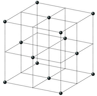
with αi(0)subscript𝛼𝑖0\alpha_{i}(0), i=1,2,3𝑖123i=1,2,3, c𝑐c, and δjsubscript𝛿𝑗\delta_{j}, j=1,2,3𝑗123j=1,2,3, being complex parameters. Figure 1.1 shows a unit cell in ΩΩ\Omega.

Refer to caption
Figure 1.1. A unit cell of the ΩΩ\Omega lattice.

Our study is motivated by two considerations. Firstly, the system (1.2) satisfies the consistency around a cuboctahedron (CACO) property [10], which is a generalization of the famous consistency around a cube (CAC) property[17]. (See Appendix A for a summary of the details of the CACO property and §1.2 for those of the CAC property.) Secondly, we are motivated by finding relations between partial difference equations and ordinary difference equations known as the discrete Painlevé equations.

In this paper, we show that the system (1.2) reduces to discrete Painlevé equations with initial value space characterised as A2(1)superscriptsubscript𝐴21A_{2}^{(1)\ast} in the sense of Sakai[22]. The latter equations have two forms in the literature given respectively by Tsuda [23] and Ramani et al. [21] and are explicitly given by:

{(Y¯+X)(X+Y)=((X+c3)2c1)((Xc3)2c2)(X+t)2c4,(X¯+Y)(X+Y)=((Yc3)2c1)((Y+c3)2c2)(Y+t+12)2c5,cases¯𝑌𝑋𝑋𝑌superscript𝑋subscript𝑐32subscript𝑐1superscript𝑋subscript𝑐32subscript𝑐2superscript𝑋𝑡2subscript𝑐4otherwise¯𝑋𝑌𝑋𝑌superscript𝑌subscript𝑐32subscript𝑐1superscript𝑌subscript𝑐32subscript𝑐2superscript𝑌𝑡122subscript𝑐5otherwise\displaystyle\begin{cases}\Big{(}\underline{Y}+X\Big{)}\Big{(}X+Y\Big{)}=\dfrac{\left((X+c_{3})^{2}-c_{1}\right)\left((X-c_{3})^{2}-c_{2}\right)}{(X+t)^{2}-c_{4}},\\ \Big{(}\overline{X}+Y)\Big{(}X+Y\Big{)}=\dfrac{\left((Y-c_{3})^{2}-c_{1}\right)\left((Y+c_{3})^{2}-c_{2}\right)}{\left(Y+t+\frac{1}{2}\right)^{2}-c_{5}},\end{cases} (1.4a)
(X¯+X)(X¯+X)=(X2c1)(X2c2)(X+t)2c3.¯𝑋𝑋¯𝑋𝑋superscript𝑋2subscript𝑐1superscript𝑋2subscript𝑐2superscript𝑋𝑡2subscript𝑐3\displaystyle\Big{(}\overline{X}+X\Big{)}\Big{(}\underline{X}+X\Big{)}=\dfrac{\left(X^{2}-c_{1}\right)\left(X^{2}-c_{2}\right)}{(X+t)^{2}-c_{3}}. (1.4b)

Here, t𝑡t\in\mathbb{C} is an independent variable, cisubscript𝑐𝑖c_{i}, i=1,5𝑖15i=1\dots,5, are complex parameters and X,Y𝑋𝑌X,Y are dependent variables:

X=X(t),Y=Y(t),X¯=X(t+1),X¯=X(t1),Y¯=Y(t1).formulae-sequence𝑋𝑋𝑡formulae-sequence𝑌𝑌𝑡formulae-sequence¯𝑋𝑋𝑡1formulae-sequence¯𝑋𝑋𝑡1¯𝑌𝑌𝑡1X=X(t),\quad Y=Y(t),\quad\overline{X}=X(t+1),\quad\underline{X}=X(t-1),\quad\underline{Y}=Y(t-1). (1.5)

We note that discrete Painlevé equations admit special solutions when parameters take special values. For example, Equation (1.4a) has the special solution given by the generalized hypergeometric series F23subscriptsubscript𝐹23{}_{3}F_{2} when 4c3+2c4+2c5=14subscript𝑐32subscript𝑐42subscript𝑐514c_{3}+2\sqrt{c_{4}}+2\sqrt{c_{5}}=1[11].

Our main result is Theorem 1.1. To state the theorem, we first explain how to take the reduction on the lattice ΩΩ\Omega. To be explicit, consider a vertex 𝒍Ω𝒍Ω{\bm{l}}\in\Omega, given by l1ϵ1+l2ϵ2+l3ϵ3subscript𝑙1subscriptitalic-ϵ1subscript𝑙2subscriptitalic-ϵ2subscript𝑙3subscriptitalic-ϵ3l_{1}\epsilon_{1}+l_{2}\epsilon_{2}+l_{3}\epsilon_{3}. Define the plane HkΩsubscript𝐻𝑘ΩH_{k}\subset\Omega given by l3=ksubscript𝑙3𝑘l_{3}=k. We project the vertices of H1subscript𝐻1H_{1} to the adjacent horizontal plane H0subscript𝐻0H_{0} by taking (l1,l2,1)(l11,l21,0)maps-tosubscript𝑙1subscript𝑙21subscript𝑙11subscript𝑙210(l_{1},l_{2},1)\mapsto(l_{1}-1,l_{2}-1,0). The union of the projection with the lattice points on H0subscript𝐻0H_{0} forms 2superscript2\mathbb{Z}^{2}. We can define such a projection from every plane Hksubscript𝐻𝑘H_{k} to H0subscript𝐻0H_{0} by the following:

(l1,l2,k)(l1k,l2k,0).maps-tosubscript𝑙1subscript𝑙2𝑘subscript𝑙1𝑘subscript𝑙2𝑘0(l_{1},l_{2},k)\mapsto(l_{1}-k,l_{2}-k,0).

We call the result of this operation a (1,1,1)111(1,1,1)-periodic reduction.

Theorem 1.1.

The A2(1)superscriptsubscript𝐴21A_{2}^{(1)\ast}-type discrete Painlevé equations (1.4) can be obtained from the system of PΔΔ\DeltaEs (1.2) via the (1,1,1)111(1,1,1)-periodic reduction.

1.1. Notation and Definitions

Throughout the paper, we use terminology to describe polynomials and quad-equations that is common in the literature. Readers who are unfamiliar with this notation may wish to consult [10, 1, 8]. We use Q=Q(x,y,z,w)𝑄𝑄𝑥𝑦𝑧𝑤Q=Q(x,y,z,w) to denote a multivariable polynomial over \mathbb{C}. Under certain conditions, i.e., that Q𝑄Q be affine linear and irreducible, we will refer to the equation Q=0𝑄0Q=0 as a quad-equation or sometimes, for succinctness, refer to the polynomial Q𝑄Q as a quad-equation. We remind the reader that the condition of irreducibility implies that Q(x,y,z,w)=0𝑄𝑥𝑦𝑧𝑤0Q(x,y,z,w)=0 can be solved for each argument, and that the solution is a rational function of the other three arguments.

1.2. Background

Integrable systems are widely applicable models of science, occurring in fluid dynamics, particle physics and optics. The prototypical example is the famous Korteweg-de Vries (KdV) equation whose solitary wave-like solutions interact elastically like particles, leading to the invention of the term soliton. It is then natural to ask what discrete versions of such equations are also integrable. This question turns out to be related to consistency conditions for polynomials associated to faces of cubes as we explain below.

Integrable discrete systems were discovered [16, 15, 20, 18] from mappings that turn out to be consistent on multi-dimensional cubes. (We note that there are additional systems that do not fall into this class, see e.g., [8, Chapter 3].) These are quad-equations in the sense in §1.1. In [1, 2, 3, 4], Adler-Bobenko-Suris et al. classified quad-equations satisfying the consistency around a cube (CAC) property, which lead integrable PΔΔ\DeltaEs. We refer to such PΔΔ\DeltaEs as ABS equations. It turns out that ABS equations contain many well known integrable PΔΔ\DeltaEs [14, 15, 16, 9].

Reductions of integrable PDEs lead to Painlevé equations, which first arose in the search for new transcendental functions in the early 1900’s[19, 6, 5]. Again a natural question is to ask whether discrete versions exist with analogous properties. This question led to the discovery of second-order difference equations called the discrete Painlevé equations[7, 13, 20]).

It is now well-known that discrete Painlevé equations have initial value spaces with geometric structures that can be identified with root systems and affine Weyl groups [22]. Sakai showed that there are 22 types of initial value spaces as shown in Table 1.1.

Table 1.1. Types of spaces of initial values.
Discrete type Type of space of initial values
Elliptic A0(1)superscriptsubscript𝐴01A_{0}^{(1)}
Multiplicative A0(1)superscriptsubscript𝐴01A_{0}^{(1)\ast}, A1(1)superscriptsubscript𝐴11A_{1}^{(1)}, A2(1)superscriptsubscript𝐴21A_{2}^{(1)}, A3(1)superscriptsubscript𝐴31A_{3}^{(1)}, …, A8(1)superscriptsubscript𝐴81A_{8}^{(1)}, A7(1)superscriptsubscript𝐴7superscript1A_{7}^{(1)^{\prime}}
Additive A0(1)superscriptsubscript𝐴01absentA_{0}^{(1)\ast\ast}, A1(1)superscriptsubscript𝐴11A_{1}^{(1)\ast}, A2(1)superscriptsubscript𝐴21A_{2}^{(1)\ast}, D4(1)superscriptsubscript𝐷41D_{4}^{(1)}, …, D8(1)superscriptsubscript𝐷81D_{8}^{(1)}, E6(1)superscriptsubscript𝐸61E_{6}^{(1)}, E7(1)superscriptsubscript𝐸71E_{7}^{(1)}, E8(1)superscriptsubscript𝐸81E_{8}^{(1)}

1.3. Outline of the paper

This paper is organized as follows. In §2, we show the extended affine Weyl group of type E6(1)superscriptsubscript𝐸61E_{6}^{(1)} and its subgroup which forms that of type A2(1)superscriptsubscript𝐴21A_{2}^{(1)}. Moreover, from those birational actions we obtain the discrete Painlevé equations (1.4) and the PΔΔ\DeltaEs (2.16), which are periodically reduced equations of the system (1.2). In §3, using the results in §2 we give the proof of Theorem 1.1. Finally, we give some concluding remarks in §4.

2. Derivation of the discrete integrable systems from an extended affine Weyl group of type E6(1)superscriptsubscript𝐸61E_{6}^{(1)}

In this section, we derive the partial/ordinary discrete integrable systems from the birational actions of an extended affine Weyl group of type E6(1)superscriptsubscript𝐸61E_{6}^{(1)}, denoted by W~(E6(1))~𝑊superscriptsubscript𝐸61\widetilde{W}(E_{6}^{(1)}). Note that details of W~(E6(1))~𝑊superscriptsubscript𝐸61\widetilde{W}(E_{6}^{(1)}) are given in Appendix B.

2.1. Extended affine Weyl group of type A2(1)superscriptsubscript𝐴21A_{2}^{(1)}

Let aisubscript𝑎𝑖a_{i}, i=0,,6𝑖06i=0,\dots,6, be parameters satisfying the condition

a1+2a2+3a3+2a4+a5+2a6+a0=1,subscript𝑎12subscript𝑎23subscript𝑎32subscript𝑎4subscript𝑎52subscript𝑎6subscript𝑎01a_{1}+2a_{2}+3a_{3}+2a_{4}+a_{5}+2a_{6}+a_{0}=1, (2.1)

and τj(i)subscriptsuperscript𝜏𝑖𝑗\tau^{(i)}_{j}, i=1,2,3𝑖123i=1,2,3, j=0,1,2,3𝑗0123j=0,1,2,3, be variables. Moreover, we define the transformations sisubscript𝑠𝑖s_{i}, i=0,,6𝑖06i=0,\dots,6, ιjsubscript𝜄𝑗\iota_{j}, j=1,2,3𝑗123j=1,2,3, by isomorphisms from the field of rational functions K({τj(i)})𝐾subscriptsuperscript𝜏𝑖𝑗K(\{\tau^{(i)}_{j}\}), where K=({ai})𝐾subscript𝑎𝑖K=\mathbb{C}(\{a_{i}\}), to itself. These transformations collectively form the extended affine Weyl group of type E6(1)superscriptsubscript𝐸61E_{6}^{(1)}, denoted by W~(E6(1))~𝑊superscriptsubscript𝐸61\widetilde{W}(E_{6}^{(1)}):

W~(E6(1))=s0,,s6ι1,ι2,ι3.~𝑊superscriptsubscript𝐸61right-normal-factor-semidirect-productsubscript𝑠0subscript𝑠6subscript𝜄1subscript𝜄2subscript𝜄3\widetilde{W}(E_{6}^{(1)})=\langle s_{0},\dots,s_{6}\rangle\rtimes\langle\iota_{1},\iota_{2},\iota_{3}\rangle. (2.2)

See Appendix B for more details.

Let us define the transformations wisubscript𝑤𝑖w_{i}, i=0,1,2𝑖012i=0,1,2, and π𝜋\pi by

w0=s2s1s3s2,w1=s4s5s3s4,w2=s6s0s3s6,π=ι3ι1.formulae-sequencesubscript𝑤0subscript𝑠2subscript𝑠1subscript𝑠3subscript𝑠2formulae-sequencesubscript𝑤1subscript𝑠4subscript𝑠5subscript𝑠3subscript𝑠4formulae-sequencesubscript𝑤2subscript𝑠6subscript𝑠0subscript𝑠3subscript𝑠6𝜋subscript𝜄3subscript𝜄1w_{0}=s_{2}s_{1}s_{3}s_{2},\quad w_{1}=s_{4}s_{5}s_{3}s_{4},\quad w_{2}=s_{6}s_{0}s_{3}s_{6},\quad\pi=\iota_{3}\iota_{1}. (2.3)

They collectively form the extended affine Weyl group of type A2(1)superscriptsubscript𝐴21A_{2}^{(1)}:

W~(A2(1))=w0,w1,w2π.~𝑊superscriptsubscript𝐴21right-normal-factor-semidirect-productsubscript𝑤0subscript𝑤1subscript𝑤2delimited-⟨⟩𝜋\widetilde{W}(A_{2}^{(1)})=\langle w_{0},w_{1},w_{2}\rangle\rtimes\langle\pi\rangle. (2.4)

Indeed, the following fundamental relations hold:

(wiwj)aij=1,i,j{0,1,2},π3=1,πw{0,1,2}=w{1,2,0}π,formulae-sequencesuperscriptsubscript𝑤𝑖subscript𝑤𝑗subscript𝑎𝑖𝑗1𝑖formulae-sequence𝑗012formulae-sequencesuperscript𝜋31𝜋subscript𝑤012subscript𝑤120𝜋(w_{i}w_{j})^{a_{ij}}=1,\quad i,j\in\{0,1,2\},\quad\pi^{3}=1,\quad\pi w_{\{0,1,2\}}=w_{\{1,2,0\}}\pi, (2.5)

where

(aij)i,j=02=(233323332).superscriptsubscriptsubscript𝑎𝑖𝑗𝑖𝑗02matrix233323332(a_{ij})_{i,j=0}^{2}=\begin{pmatrix}2&3&3\\[-8.00003pt] 3&2&3\\[-8.00003pt] 3&3&2\end{pmatrix}. (2.6)

Introduce the parameters and variables that go well with W~(A2(1))~𝑊superscriptsubscript𝐴21\widetilde{W}(A_{2}^{(1)}) as follows. Let

b0=a1+2a2+a3,b1=a3+2a4+a5,b2=a3+2a6+a0,formulae-sequencesubscript𝑏0subscript𝑎12subscript𝑎2subscript𝑎3formulae-sequencesubscript𝑏1subscript𝑎32subscript𝑎4subscript𝑎5subscript𝑏2subscript𝑎32subscript𝑎6subscript𝑎0\displaystyle b_{0}=a_{1}+2a_{2}+a_{3},\quad b_{1}=a_{3}+2a_{4}+a_{5},\quad b_{2}=a_{3}+2a_{6}+a_{0}, (2.7a)
c=a0+a1+a3+a52,d12=a0+a1a3a52,d23=a0a1+a3a52,formulae-sequence𝑐subscript𝑎0subscript𝑎1subscript𝑎3subscript𝑎52formulae-sequencesubscript𝑑12subscript𝑎0subscript𝑎1subscript𝑎3subscript𝑎52subscript𝑑23subscript𝑎0subscript𝑎1subscript𝑎3subscript𝑎52\displaystyle c=\dfrac{a_{0}+a_{1}+a_{3}+a_{5}}{2},\quad d_{12}=\dfrac{a_{0}+a_{1}-a_{3}-a_{5}}{2},\quad d_{23}=\dfrac{a_{0}-a_{1}+a_{3}-a_{5}}{2}, (2.7b)
d13=a0a1a3+a52,subscript𝑑13subscript𝑎0subscript𝑎1subscript𝑎3subscript𝑎52\displaystyle d_{13}=\dfrac{a_{0}-a_{1}-a_{3}+a_{5}}{2}, (2.7c)

where b0+b1+b2=1subscript𝑏0subscript𝑏1subscript𝑏21b_{0}+b_{1}+b_{2}=1, and

y1=τ1(1)τ0(1),y2=τ3(3)τ2(3),y3=τ1(2)τ0(2),y4=τ3(2)τ2(2),y5=τ3(1)τ2(1),y6=τ1(3)τ0(3).formulae-sequencesubscript𝑦1subscriptsuperscript𝜏11subscriptsuperscript𝜏10formulae-sequencesubscript𝑦2subscriptsuperscript𝜏33subscriptsuperscript𝜏32formulae-sequencesubscript𝑦3subscriptsuperscript𝜏21subscriptsuperscript𝜏20formulae-sequencesubscript𝑦4subscriptsuperscript𝜏23subscriptsuperscript𝜏22formulae-sequencesubscript𝑦5subscriptsuperscript𝜏13subscriptsuperscript𝜏12subscript𝑦6subscriptsuperscript𝜏31subscriptsuperscript𝜏30y_{1}=\frac{\tau^{(1)}_{1}}{\tau^{(1)}_{0}},\quad y_{2}=\frac{\tau^{(3)}_{3}}{\tau^{(3)}_{2}},\quad y_{3}=\frac{\tau^{(2)}_{1}}{\tau^{(2)}_{0}},\quad y_{4}=\frac{\tau^{(2)}_{3}}{\tau^{(2)}_{2}},\quad y_{5}=\frac{\tau^{(1)}_{3}}{\tau^{(1)}_{2}},\quad y_{6}=\frac{\tau^{(3)}_{1}}{\tau^{(3)}_{0}}. (2.8)

Then, the action of W~(A2(1))~𝑊superscriptsubscript𝐴21\widetilde{W}(A_{2}^{(1)}) on the parameters b0subscript𝑏0b_{0}, b1subscript𝑏1b_{1}, b2subscript𝑏2b_{2}, c𝑐c, d12subscript𝑑12d_{12}, d23subscript𝑑23d_{23}, d13subscript𝑑13d_{13} are given by

wi(bj)={biif i=j,bj+biif ij,w0:(d12,d23)(d23,d12),:subscript𝑤𝑖subscript𝑏𝑗casessubscript𝑏𝑖if 𝑖𝑗subscript𝑏𝑗subscript𝑏𝑖if 𝑖𝑗subscript𝑤0maps-tosubscript𝑑12subscript𝑑23subscript𝑑23subscript𝑑12\displaystyle w_{i}(b_{j})=\begin{cases}-b_{i}&\text{if }~{}i=j,\\ b_{j}+b_{i}&\text{if }~{}i\neq j,\end{cases}\qquad w_{0}:(d_{12},d_{23})\mapsto(d_{23},d_{12}), (2.9a)
w1:(d23,d13)(d13,d23),w2:(d12,d13)(d13,d12),:subscript𝑤1maps-tosubscript𝑑23subscript𝑑13subscript𝑑13subscript𝑑23subscript𝑤2:maps-tosubscript𝑑12subscript𝑑13subscript𝑑13subscript𝑑12\displaystyle w_{1}:(d_{23},d_{13})\mapsto(d_{13},d_{23}),\qquad w_{2}:(d_{12},d_{13})\mapsto(-d_{13},-d_{12}), (2.9b)
π:(b0,b1,b2,d12,d23,d13)(b1,b2,b0,d23,d13,d12),:𝜋maps-tosubscript𝑏0subscript𝑏1subscript𝑏2subscript𝑑12subscript𝑑23subscript𝑑13subscript𝑏1subscript𝑏2subscript𝑏0subscript𝑑23subscript𝑑13subscript𝑑12\displaystyle\pi:(b_{0},b_{1},b_{2},d_{12},d_{23},d_{13})\mapsto(b_{1},b_{2},b_{0},-d_{23},-d_{13},d_{12}), (2.9c)

where i,j/(3)𝑖𝑗3i,j\in\mathbb{Z}/(3\mathbb{Z}), while those on the y𝑦y-variables yisubscript𝑦𝑖y_{i}, i=1,,6𝑖16i=1,\dots,6, are given by

w0:(y1,y3y5,y6)(y5,(b0c+d13)y3(b0d12+d23)y1(b0+d12d23)y3(b0+cd13)y1y5y1,(b0c+d13)y6(b0d12+d23)y1(b0+d12d23)y6(b0+cd13)y1y5),:subscript𝑤0maps-tomatrixsubscript𝑦1subscript𝑦3subscript𝑦5subscript𝑦6matrixsubscript𝑦5subscript𝑏0𝑐subscript𝑑13subscript𝑦3subscript𝑏0subscript𝑑12subscript𝑑23subscript𝑦1subscript𝑏0subscript𝑑12subscript𝑑23subscript𝑦3subscript𝑏0𝑐subscript𝑑13subscript𝑦1subscript𝑦5subscript𝑦1subscript𝑏0𝑐subscript𝑑13subscript𝑦6subscript𝑏0subscript𝑑12subscript𝑑23subscript𝑦1subscript𝑏0subscript𝑑12subscript𝑑23subscript𝑦6subscript𝑏0𝑐subscript𝑑13subscript𝑦1subscript𝑦5\displaystyle w_{0}:\begin{pmatrix}y_{1},~{}y_{3}\\ y_{5},~{}y_{6}\end{pmatrix}\mapsto\left(\begin{matrix}y_{5},~{}\dfrac{(b_{0}-c+d_{13})y_{3}-(b_{0}-d_{12}+d_{23})y_{1}}{(b_{0}+d_{12}-d_{23})y_{3}-(b_{0}+c-d_{13})y_{1}}y_{5}\\[15.00002pt] y_{1},~{}\dfrac{(b_{0}-c+d_{13})y_{6}-(b_{0}-d_{12}+d_{23})y_{1}}{(b_{0}+d_{12}-d_{23})y_{6}-(b_{0}+c-d_{13})y_{1}}y_{5}\end{matrix}\right), (2.10a)
w1:(y1,y3y4,y6)((b1c+d12)y1(b1d13+d23)y3(b1+d13d23)y1(b1+cd12)y3y4,y4y3,(b1c+d12)y6(b1d13+d23)y3(b1+d13d23)y6(b1+cd12)y3y4),:subscript𝑤1maps-tomatrixsubscript𝑦1subscript𝑦3subscript𝑦4subscript𝑦6matrixsubscript𝑏1𝑐subscript𝑑12subscript𝑦1subscript𝑏1subscript𝑑13subscript𝑑23subscript𝑦3subscript𝑏1subscript𝑑13subscript𝑑23subscript𝑦1subscript𝑏1𝑐subscript𝑑12subscript𝑦3subscript𝑦4subscript𝑦4subscript𝑦3subscript𝑏1𝑐subscript𝑑12subscript𝑦6subscript𝑏1subscript𝑑13subscript𝑑23subscript𝑦3subscript𝑏1subscript𝑑13subscript𝑑23subscript𝑦6subscript𝑏1𝑐subscript𝑑12subscript𝑦3subscript𝑦4\displaystyle w_{1}:\begin{pmatrix}y_{1},~{}y_{3}\\ y_{4},~{}y_{6}\end{pmatrix}\mapsto\left(\begin{matrix}\dfrac{(b_{1}-c+d_{12})y_{1}-(b_{1}-d_{13}+d_{23})y_{3}}{(b_{1}+d_{13}-d_{23})y_{1}-(b_{1}+c-d_{12})y_{3}}y_{4},~{}y_{4}\\[15.00002pt] y_{3},~{}\dfrac{(b_{1}-c+d_{12})y_{6}-(b_{1}-d_{13}+d_{23})y_{3}}{(b_{1}+d_{13}-d_{23})y_{6}-(b_{1}+c-d_{12})y_{3}}y_{4}\end{matrix}\right), (2.10b)
w2:(y1,y2y3,y6)((b2cd23)y1(b2d12d13)y6(b2+d12+d13)y1(b2+c+d23)y6y2,y6(b2d12d13)y6(b2cd23)y3(b2+c+d23)y6(b2+d12+d13)y3y2,y2),:subscript𝑤2maps-tomatrixsubscript𝑦1subscript𝑦2subscript𝑦3subscript𝑦6matrixsubscript𝑏2𝑐subscript𝑑23subscript𝑦1subscript𝑏2subscript𝑑12subscript𝑑13subscript𝑦6subscript𝑏2subscript𝑑12subscript𝑑13subscript𝑦1subscript𝑏2𝑐subscript𝑑23subscript𝑦6subscript𝑦2subscript𝑦6subscript𝑏2subscript𝑑12subscript𝑑13subscript𝑦6subscript𝑏2𝑐subscript𝑑23subscript𝑦3subscript𝑏2𝑐subscript𝑑23subscript𝑦6subscript𝑏2subscript𝑑12subscript𝑑13subscript𝑦3subscript𝑦2subscript𝑦2\displaystyle w_{2}:\begin{pmatrix}y_{1},~{}y_{2}\\ y_{3},~{}y_{6}\end{pmatrix}\mapsto\left(\begin{matrix}\dfrac{(b_{2}-c-d_{23})y_{1}-(b_{2}-d_{12}-d_{13})y_{6}}{(b_{2}+d_{12}+d_{13})y_{1}-(b_{2}+c+d_{23})y_{6}}y_{2},~{}y_{6}\\[15.00002pt] \dfrac{(b_{2}-d_{12}-d_{13})y_{6}-(b_{2}-c-d_{23})y_{3}}{(b_{2}+c+d_{23})y_{6}-(b_{2}+d_{12}+d_{13})y_{3}}y_{2},~{}y_{2}\end{matrix}\right), (2.10c)
π:(y1,y2,y3,y4,y5,y6)(y3,y5,y6,y2,y4,y1).:𝜋maps-tosubscript𝑦1subscript𝑦2subscript𝑦3subscript𝑦4subscript𝑦5subscript𝑦6subscript𝑦3subscript𝑦5subscript𝑦6subscript𝑦2subscript𝑦4subscript𝑦1\displaystyle\pi:(y_{1},y_{2},y_{3},y_{4},y_{5},y_{6})\mapsto(y_{3},y_{5},y_{6},y_{2},y_{4},y_{1}). (2.10d)
Remark 2.1.

We follow the convention that the parameters and y𝑦y-variables not explicitly included in the actions listed in Equations (2.9) and (2.10) are the ones that remain unchanged under the action of the corresponding transformation. That is, the transformation acts as an identity on those parameters or variables.

For later convenience, we here define the translations in W~(A2(1))~𝑊superscriptsubscript𝐴21\widetilde{W}(A_{2}^{(1)}) by

T1=w1w2π2,T2=w2w0π2,T3=w0w1π2,formulae-sequencesubscript𝑇1subscript𝑤1subscript𝑤2superscript𝜋2formulae-sequencesubscript𝑇2subscript𝑤2subscript𝑤0superscript𝜋2subscript𝑇3subscript𝑤0subscript𝑤1superscript𝜋2T_{1}=w_{1}w_{2}\pi^{2},\quad T_{2}=w_{2}w_{0}\pi^{2},\quad T_{3}=w_{0}w_{1}\pi^{2}, (2.11)

whose actions on the parameters b0subscript𝑏0b_{0}, b1subscript𝑏1b_{1}, b2subscript𝑏2b_{2}, c𝑐c, d12subscript𝑑12d_{12}, d23subscript𝑑23d_{23}, d13subscript𝑑13d_{13} are given by

T1::subscript𝑇1absent\displaystyle T_{1}: (b0,b1,d12,d13)(b01,b1+1,d12,d13),maps-tosubscript𝑏0subscript𝑏1subscript𝑑12subscript𝑑13subscript𝑏01subscript𝑏11subscript𝑑12subscript𝑑13\displaystyle(b_{0},b_{1},d_{12},d_{13})\mapsto(b_{0}-1,b_{1}+1,-d_{12},-d_{13}), (2.12a)
T2::subscript𝑇2absent\displaystyle T_{2}: (b1,b2,d12,d23)(b11,b2+1,d12,d23),maps-tosubscript𝑏1subscript𝑏2subscript𝑑12subscript𝑑23subscript𝑏11subscript𝑏21subscript𝑑12subscript𝑑23\displaystyle(b_{1},b_{2},d_{12},d_{23})\mapsto(b_{1}-1,b_{2}+1,-d_{12},-d_{23}), (2.12b)
T3::subscript𝑇3absent\displaystyle T_{3}: (b2,b0,d23,d13)(b21,b0+1,d23,d13).maps-tosubscript𝑏2subscript𝑏0subscript𝑑23subscript𝑑13subscript𝑏21subscript𝑏01subscript𝑑23subscript𝑑13\displaystyle(b_{2},b_{0},d_{23},d_{13})\mapsto(b_{2}-1,b_{0}+1,-d_{23},-d_{13}). (2.12c)

Note that T1T2T3=1subscript𝑇1subscript𝑇2subscript𝑇31T_{1}T_{2}T_{3}=1 and TiTj=TjTisubscript𝑇𝑖subscript𝑇𝑗subscript𝑇𝑗subscript𝑇𝑖T_{i}T_{j}=T_{j}T_{i}, where i,j=1,2,3formulae-sequence𝑖𝑗123i,j=1,2,3, hold.

2.2. Derivation of the partial difference equations from W~(A2(1))~𝑊superscriptsubscript𝐴21\widetilde{W}(A_{2}^{(1)})

In this subsection, we derive the PΔΔ\DeltaEs (2.16) from the birational action of W~(A2(1))~𝑊superscriptsubscript𝐴21\widetilde{W}(A_{2}^{(1)}).

Let

ul1,l2,l3=T1l1T2l2T3l3(y2).subscript𝑢subscript𝑙1subscript𝑙2subscript𝑙3superscriptsubscript𝑇1subscript𝑙1superscriptsubscript𝑇2subscript𝑙2superscriptsubscript𝑇3subscript𝑙3subscript𝑦2u_{l_{1},l_{2},l_{3}}={T_{1}}^{l_{1}}{T_{2}}^{l_{2}}{T_{3}}^{l_{3}}(y_{2}). (2.13)

Note that

u0,1,1=y1,u0,0,0=y2,u1,0,0=y3,u0,1,0=y4,u1,1,0=y5,u1,2,0=y6.formulae-sequencesubscript𝑢011subscript𝑦1formulae-sequencesubscript𝑢000subscript𝑦2formulae-sequencesubscript𝑢100subscript𝑦3formulae-sequencesubscript𝑢010subscript𝑦4formulae-sequencesubscript𝑢110subscript𝑦5subscript𝑢120subscript𝑦6u_{0,1,1}=y_{1},\quad u_{0,0,0}=y_{2},\quad u_{1,0,0}=y_{3},\quad u_{0,1,0}=y_{4},\quad u_{1,1,0}=y_{5},\quad u_{1,2,0}=y_{6}. (2.14)

We assign the variable ul1,l2,l3subscript𝑢subscript𝑙1subscript𝑙2subscript𝑙3u_{l_{1},l_{2},l_{3}} on the vertices (l1,l2,l3)subscript𝑙1subscript𝑙2subscript𝑙3(l_{1},l_{2},l_{3}) of the triangle lattice

3/(1,1,1):={(l1,l2,l3)3|l1+l2+l3=0}.assignsuperscript3111conditional-setsubscript𝑙1subscript𝑙2subscript𝑙3superscript3subscript𝑙1subscript𝑙2subscript𝑙30\mathbb{Z}^{3}/(1,1,1):=\left\{\left.(l_{1},l_{2},l_{3})\in\mathbb{Z}^{3}~{}\right|~{}l_{1}+l_{2}+l_{3}=0\right\}. (2.15)

Then, we obtain the following lemma.

Lemma 2.2.

On the triangle lattice there are three fundamental relations (essentially two):

ui¯ui¯=(bli,lj(i)c+(1)li+ljdij)uj¯(bli,lj(i)(1)lj+lkdjk+(1)li+lkdik)uj¯(bli,lj(i)+(1)lj+lkdjk(1)li+lkdik)uj¯(bli,lj(i)+c(1)li+ljdij)uj¯,subscript𝑢¯𝑖subscript𝑢¯𝑖subscriptsuperscript𝑏𝑖subscript𝑙𝑖subscript𝑙𝑗𝑐superscript1subscript𝑙𝑖subscript𝑙𝑗subscript𝑑𝑖𝑗subscript𝑢¯𝑗subscriptsuperscript𝑏𝑖subscript𝑙𝑖subscript𝑙𝑗superscript1subscript𝑙𝑗subscript𝑙𝑘subscript𝑑𝑗𝑘superscript1subscript𝑙𝑖subscript𝑙𝑘subscript𝑑𝑖𝑘subscript𝑢¯𝑗subscriptsuperscript𝑏𝑖subscript𝑙𝑖subscript𝑙𝑗superscript1subscript𝑙𝑗subscript𝑙𝑘subscript𝑑𝑗𝑘superscript1subscript𝑙𝑖subscript𝑙𝑘subscript𝑑𝑖𝑘subscript𝑢¯𝑗subscriptsuperscript𝑏𝑖subscript𝑙𝑖subscript𝑙𝑗𝑐superscript1subscript𝑙𝑖subscript𝑙𝑗subscript𝑑𝑖𝑗subscript𝑢¯𝑗\dfrac{u_{\overline{i}}}{u_{\underline{i}}}=\dfrac{\Big{(}b^{(i)}_{l_{i},l_{j}}-c+(-1)^{l_{i}+l_{j}}d_{ij}\Big{)}u_{\overline{j}}-\Big{(}b^{(i)}_{l_{i},l_{j}}-(-1)^{l_{j}+l_{k}}d_{jk}+(-1)^{l_{i}+l_{k}}d_{ik}\Big{)}u_{\underline{j}}}{\Big{(}b^{(i)}_{l_{i},l_{j}}+(-1)^{l_{j}+l_{k}}d_{jk}-(-1)^{l_{i}+l_{k}}d_{ik}\Big{)}u_{\overline{j}}-\Big{(}b^{(i)}_{l_{i},l_{j}}+c-(-1)^{l_{i}+l_{j}}d_{ij}\Big{)}u_{\underline{j}}}, (2.16)

where (i,j,k)=(1,2,3),(2,3,1),(3,1,2)𝑖𝑗𝑘123231312(i,j,k)=(1,2,3),\,(2,3,1),\,(3,1,2) and

bl1,l2(1)=b1+l1l2,bl2,l3(2)=b2+l2l31,bl1,l3(0)=b0+l3l1.formulae-sequencesubscriptsuperscript𝑏1subscript𝑙1subscript𝑙2subscript𝑏1subscript𝑙1subscript𝑙2formulae-sequencesubscriptsuperscript𝑏2subscript𝑙2subscript𝑙3subscript𝑏2subscript𝑙2subscript𝑙31subscriptsuperscript𝑏0subscript𝑙1subscript𝑙3subscript𝑏0subscript𝑙3subscript𝑙1b^{(1)}_{l_{1},l_{2}}=b_{1}+l_{1}-l_{2},\quad b^{(2)}_{l_{2},l_{3}}=b_{2}+l_{2}-l_{3}-1,\quad b^{(0)}_{l_{1},l_{3}}=b_{0}+l_{3}-l_{1}. (2.17)

Here, u=ul1,l2,l3𝑢subscript𝑢subscript𝑙1subscript𝑙2subscript𝑙3u=u_{l_{1},l_{2},l_{3}} and the subscript  i¯¯𝑖{\overline{i}} (or, i¯¯𝑖\underline{i} ) for a function u=ul1,l2,l3𝑢subscript𝑢subscript𝑙1subscript𝑙2subscript𝑙3u=u_{l_{1},l_{2},l_{3}} means  +11+1 shift (or, 11-1 shift) in the lisubscript𝑙𝑖l_{i}-direction.

Proof.

Equations (2.16) with (i,j,k)=(1,2,3),(2,3,1),(3,1,2)𝑖𝑗𝑘123231312(i,j,k)=(1,2,3),\,(2,3,1),\,(3,1,2) are respectively obtained from the following actions:

T1(y5)y4=(b1c+d12)y6(b1+d23d13)y3(b1d23+d13)y6(b1+cd12)y3,subscript𝑇1subscript𝑦5subscript𝑦4subscript𝑏1𝑐subscript𝑑12subscript𝑦6subscript𝑏1subscript𝑑23subscript𝑑13subscript𝑦3subscript𝑏1subscript𝑑23subscript𝑑13subscript𝑦6subscript𝑏1𝑐subscript𝑑12subscript𝑦3\displaystyle\dfrac{T_{1}(y_{5})}{y_{4}}=\dfrac{(b_{1}-c+d_{12})y_{6}-(b_{1}+d_{23}-d_{13})y_{3}}{(b_{1}-d_{23}+d_{13})y_{6}-(b_{1}+c-d_{12})y_{3}}, (2.18a)
T2(y4)y2=(b2cd23)y1(b2d13d12)y6(b2+d13+d12)y1(b2+c+d23)y6,subscript𝑇2subscript𝑦4subscript𝑦2subscript𝑏2𝑐subscript𝑑23subscript𝑦1subscript𝑏2subscript𝑑13subscript𝑑12subscript𝑦6subscript𝑏2subscript𝑑13subscript𝑑12subscript𝑦1subscript𝑏2𝑐subscript𝑑23subscript𝑦6\displaystyle\dfrac{T_{2}(y_{4})}{y_{2}}=\dfrac{(b_{2}-c-d_{23})y_{1}-(b_{2}-d_{13}-d_{12})y_{6}}{(b_{2}+d_{13}+d_{12})y_{1}-(b_{2}+c+d_{23})y_{6}}, (2.18b)
T3(y2)y5=(b0c+d13)y3(b0d12+d23)y1(b0+d12d23)y3(b0+cd13)y1.subscript𝑇3subscript𝑦2subscript𝑦5subscript𝑏0𝑐subscript𝑑13subscript𝑦3subscript𝑏0subscript𝑑12subscript𝑑23subscript𝑦1subscript𝑏0subscript𝑑12subscript𝑑23subscript𝑦3subscript𝑏0𝑐subscript𝑑13subscript𝑦1\displaystyle\dfrac{T_{3}(y_{2})}{y_{5}}=\dfrac{(b_{0}-c+d_{13})y_{3}-(b_{0}-d_{12}+d_{23})y_{1}}{(b_{0}+d_{12}-d_{23})y_{3}-(b_{0}+c-d_{13})y_{1}}. (2.18c)

Moreover, we can easily verify that using Equations (2.16) we can express any ul1,l2,l3subscript𝑢subscript𝑙1subscript𝑙2subscript𝑙3u_{l_{1},l_{2},l_{3}} on the lattice by the six initial variables yisubscript𝑦𝑖y_{i}, i=1,,6𝑖16i=1,\dots,6, and one of the equations (2.16) can be obtained from the other two equations. Therefore, we have completed the proof. ∎

Remark 2.3.

Because of the following relations:

w0(ul1,l2,l3)=ul3,l2,l1,w1(ul1,l2,l3)=ul2,l1,l3,w2(ul1,l2,l3)=ul1+1,l3+2,l2,formulae-sequencesubscript𝑤0subscript𝑢subscript𝑙1subscript𝑙2subscript𝑙3subscript𝑢subscript𝑙3subscript𝑙2subscript𝑙1formulae-sequencesubscript𝑤1subscript𝑢subscript𝑙1subscript𝑙2subscript𝑙3subscript𝑢subscript𝑙2subscript𝑙1subscript𝑙3subscript𝑤2subscript𝑢subscript𝑙1subscript𝑙2subscript𝑙3subscript𝑢subscript𝑙11subscript𝑙32subscript𝑙2\displaystyle w_{0}(u_{l_{1},l_{2},l_{3}})=u_{l_{3},l_{2},l_{1}}\,,\quad w_{1}(u_{l_{1},l_{2},l_{3}})=u_{l_{2},l_{1},l_{3}}\,,\quad w_{2}(u_{l_{1},l_{2},l_{3}})=u_{l_{1}+1,l_{3}+2,l_{2}}\,, (2.19a)
π(ul1,l2,l3)=ul3+1,l1+1,l2,𝜋subscript𝑢subscript𝑙1subscript𝑙2subscript𝑙3subscript𝑢subscript𝑙31subscript𝑙11subscript𝑙2\displaystyle\pi(u_{l_{1},l_{2},l_{3}})=u_{l_{3}+1,l_{1}+1,l_{2}}\,, (2.19b)

which follow from

w0T{1,2,3}=T{3,2,1}w0,w1T{1,2,3}=T{2,1,3}w1,w2T{1,2,3}=T{1,3,2}w2,formulae-sequencesubscript𝑤0subscript𝑇123subscript𝑇321subscript𝑤0formulae-sequencesubscript𝑤1subscript𝑇123subscript𝑇213subscript𝑤1subscript𝑤2subscript𝑇123subscript𝑇132subscript𝑤2\displaystyle w_{0}T_{\{1,2,3\}}=T_{\{3,2,1\}}w_{0},\quad w_{1}T_{\{1,2,3\}}=T_{\{2,1,3\}}w_{1},\quad w_{2}T_{\{1,2,3\}}=T_{\{1,3,2\}}w_{2}, (2.20a)
πT{1,2,3}=T{2,3,1}π,w0(u0,0,0)=u0,0,0,w1(u0,0,0)=u0,0,0,formulae-sequence𝜋subscript𝑇123subscript𝑇231𝜋formulae-sequencesubscript𝑤0subscript𝑢000subscript𝑢000subscript𝑤1subscript𝑢000subscript𝑢000\displaystyle\pi T_{\{1,2,3\}}=T_{\{2,3,1\}}\pi,\quad w_{0}(u_{0,0,0})=u_{0,0,0},\quad w_{1}(u_{0,0,0})=u_{0,0,0}, (2.20b)
w2(u0,0,0)=u1,2,0,π(u0,0,0)=u1,1,0,formulae-sequencesubscript𝑤2subscript𝑢000subscript𝑢120𝜋subscript𝑢000subscript𝑢110\displaystyle w_{2}(u_{0,0,0})=u_{1,2,0},\quad\pi(u_{0,0,0})=u_{1,1,0}, (2.20c)

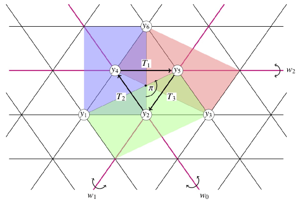
the transformation group W~(A2(1))~𝑊superscriptsubscript𝐴21\widetilde{W}(A_{2}^{(1)}) can be also regarded as the symmetry of the triangle lattice (see Figure 2.1).
Refer to caption
Figure 2.1. Triangle lattice. On the vertices the variables ul1,l2,l3subscript𝑢subscript𝑙1subscript𝑙2subscript𝑙3u_{l_{1},l_{2},l_{3}} are assigned, and on the quadrilaterals there exist quad-equations (2.16), e.g. Equations (2.18a), (2.18b) and (2.18c) are colored in red, blue and green, respectively.

2.3. Derivation of the A2(1)superscriptsubscript𝐴21A_{2}^{(1)\ast}-type discrete Painlevé equations from W~(A2(1))~𝑊superscriptsubscript𝐴21\widetilde{W}(A_{2}^{(1)})

In this subsection, we derive the A2(1)superscriptsubscript𝐴21A_{2}^{(1)\ast}-type discrete Painlevé equations (1.4) from the birational action of W~(A2(1))~𝑊superscriptsubscript𝐴21\widetilde{W}(A_{2}^{(1)}).

Let

f=(cd12+d23d13)y12(y6y1)+b2+cd12+d23d134,𝑓𝑐subscript𝑑12subscript𝑑23subscript𝑑13subscript𝑦12subscript𝑦6subscript𝑦1subscript𝑏2𝑐subscript𝑑12subscript𝑑23subscript𝑑134\displaystyle f=\dfrac{(c-d_{12}+d_{23}-d_{13})y_{1}}{2(y_{6}-y_{1})}+\frac{b_{2}+c-d_{12}+d_{23}-d_{13}}{4}, (2.21a)
g=(cd12+d23d13)y32(y3y6)b2+cd12+d23d134.𝑔𝑐subscript𝑑12subscript𝑑23subscript𝑑13subscript𝑦32subscript𝑦3subscript𝑦6subscript𝑏2𝑐subscript𝑑12subscript𝑑23subscript𝑑134\displaystyle g=\dfrac{(c-d_{12}+d_{23}-d_{13})y_{3}}{2(y_{3}-y_{6})}-\frac{b_{2}+c-d_{12}+d_{23}-d_{13}}{4}. (2.21b)

Then, the action of W~(A2(1))~𝑊superscriptsubscript𝐴21\widetilde{W}(A_{2}^{(1)}) on the variables f𝑓f and g𝑔g are given by

w0(f)=fb04,w1(g)=g+b14,π(g)=fb2+b04,formulae-sequencesubscript𝑤0𝑓𝑓subscript𝑏04formulae-sequencesubscript𝑤1𝑔𝑔subscript𝑏14𝜋𝑔𝑓subscript𝑏2subscript𝑏04\displaystyle w_{0}(f)=f-\frac{b_{0}}{4},\quad w_{1}(g)=g+\frac{b_{1}}{4},\quad\pi(g)=f-\frac{b_{2}+b_{0}}{4}, (2.22a)
4(cd12+d23d13)4f2b0b2cd12+d23+d13(w0(g)+b2+b0+c+d12d23d134)4𝑐subscript𝑑12subscript𝑑23subscript𝑑134𝑓2subscript𝑏0subscript𝑏2𝑐subscript𝑑12subscript𝑑23subscript𝑑13subscript𝑤0𝑔subscript𝑏2subscript𝑏0𝑐subscript𝑑12subscript𝑑23subscript𝑑134\displaystyle\frac{4(c-d_{12}+d_{23}-d_{13})}{4f-2b_{0}-b_{2}-c-d_{12}+d_{23}+d_{13}}\left(w_{0}(g)+\frac{b_{2}+b_{0}+c+d_{12}-d_{23}-d_{13}}{4}\right)
=(b0d12+d23)(4g+b2c+d12d23+d13)4fb2+cd12+d23d13absentsubscript𝑏0subscript𝑑12subscript𝑑234𝑔subscript𝑏2𝑐subscript𝑑12subscript𝑑23subscript𝑑134𝑓subscript𝑏2𝑐subscript𝑑12subscript𝑑23subscript𝑑13\displaystyle\hskip 10.00002pt=\frac{(b_{0}-d_{12}+d_{23})(4g+b_{2}-c+d_{12}-d_{23}+d_{13})}{4f-b_{2}+c-d_{12}+d_{23}-d_{13}}
(b0c+d13)(4g+b2+cd12+d23d13)4fb2c+d12d23+d13,subscript𝑏0𝑐subscript𝑑134𝑔subscript𝑏2𝑐subscript𝑑12subscript𝑑23subscript𝑑134𝑓subscript𝑏2𝑐subscript𝑑12subscript𝑑23subscript𝑑13\displaystyle\hskip 25.00003pt-\frac{(b_{0}-c+d_{13})(4g+b_{2}+c-d_{12}+d_{23}-d_{13})}{4f-b_{2}-c+d_{12}-d_{23}+d_{13}}, (2.22b)
4(cd12+d23d13)4g+2b1+b2+cd12d23+d13(w1(f)b1+b2+cd12d23+d134)4𝑐subscript𝑑12subscript𝑑23subscript𝑑134𝑔2subscript𝑏1subscript𝑏2𝑐subscript𝑑12subscript𝑑23subscript𝑑13subscript𝑤1𝑓subscript𝑏1subscript𝑏2𝑐subscript𝑑12subscript𝑑23subscript𝑑134\displaystyle\frac{4(c-d_{12}+d_{23}-d_{13})}{4g+2b_{1}+b_{2}+c-d_{12}-d_{23}+d_{13}}\left(w_{1}(f)-\frac{b_{1}+b_{2}+c-d_{12}-d_{23}+d_{13}}{4}\right)
=(b1+d23d13)(4fb2+cd12+d23d13)4g+b2c+d12d23+d13absentsubscript𝑏1subscript𝑑23subscript𝑑134𝑓subscript𝑏2𝑐subscript𝑑12subscript𝑑23subscript𝑑134𝑔subscript𝑏2𝑐subscript𝑑12subscript𝑑23subscript𝑑13\displaystyle\hskip 10.00002pt=\frac{(b_{1}+d_{23}-d_{13})(4f-b_{2}+c-d_{12}+d_{23}-d_{13})}{4g+b_{2}-c+d_{12}-d_{23}+d_{13}}
(b1c+d12)(4fb2c+d12d23+d13)4g+b2+cd12+d23d13,subscript𝑏1𝑐subscript𝑑124𝑓subscript𝑏2𝑐subscript𝑑12subscript𝑑23subscript𝑑134𝑔subscript𝑏2𝑐subscript𝑑12subscript𝑑23subscript𝑑13\displaystyle\hskip 25.00003pt-\frac{(b_{1}-c+d_{12})(4f-b_{2}-c+d_{12}-d_{23}+d_{13})}{4g+b_{2}+c-d_{12}+d_{23}-d_{13}}, (2.22c)
π(f)=(4fb2+cd12+d23d13)(4g+b2+cd12+d23d13)16(f+g)𝜋𝑓4𝑓subscript𝑏2𝑐subscript𝑑12subscript𝑑23subscript𝑑134𝑔subscript𝑏2𝑐subscript𝑑12subscript𝑑23subscript𝑑1316𝑓𝑔\displaystyle\pi(f)=-\frac{(4f-b_{2}+c-d_{12}+d_{23}-d_{13})(4g+b_{2}+c-d_{12}+d_{23}-d_{13})}{16(f+g)}
+b0+cd12+d23d134.subscript𝑏0𝑐subscript𝑑12subscript𝑑23subscript𝑑134\displaystyle\hskip 30.00005pt+\frac{b_{0}+c-d_{12}+d_{23}-d_{13}}{4}. (2.22d)

Using the transformation T12superscriptsubscript𝑇12{T_{1}}^{2} whose action on the parameter space {b0,b1,b2,c,d12,d23,d13}subscript𝑏0subscript𝑏1subscript𝑏2𝑐subscript𝑑12subscript𝑑23subscript𝑑13\{b_{0},b_{1},b_{2},c,d_{12},d_{23},d_{13}\} is translational as T12:(b0,b1)(b02,b1+2):superscriptsubscript𝑇12maps-tosubscript𝑏0subscript𝑏1subscript𝑏02subscript𝑏12{T_{1}}^{2}:(b_{0},b_{1})\mapsto(b_{0}-2,b_{1}+2) shows, we obtain the discrete Painlevé equation (1.4a) with the following correspondence:

X=f,Y=g,X¯=T12(f),Y¯=T12(g),t=2b1+b224,formulae-sequence𝑋𝑓formulae-sequence𝑌𝑔formulae-sequence¯𝑋superscriptsubscript𝑇12𝑓formulae-sequence¯𝑌superscriptsubscript𝑇12𝑔𝑡2subscript𝑏1subscript𝑏224\displaystyle X=f,\quad Y=g,\quad\overline{X}={T_{1}}^{2}(f),\quad\underline{Y}={T_{1}}^{-2}(g),\quad t=\dfrac{2b_{1}+b_{2}-2}{4}, (2.23a)
c1=(b2+c+d23)216,c2=(b2cd23)216,c3=d12+d134,formulae-sequencesubscript𝑐1superscriptsubscript𝑏2𝑐subscript𝑑23216formulae-sequencesubscript𝑐2superscriptsubscript𝑏2𝑐subscript𝑑23216subscript𝑐3subscript𝑑12subscript𝑑134\displaystyle c_{1}=\dfrac{(b_{2}+c+d_{23})^{2}}{16},\quad c_{2}=\dfrac{(b_{2}-c-d_{23})^{2}}{16},\quad c_{3}=\dfrac{d_{12}+d_{13}}{4}, (2.23b)
c4=(c+d12d23d13)216,c5=(cd12d23+d13)216.formulae-sequencesubscript𝑐4superscript𝑐subscript𝑑12subscript𝑑23subscript𝑑13216subscript𝑐5superscript𝑐subscript𝑑12subscript𝑑23subscript𝑑13216\displaystyle c_{4}=\dfrac{(c+d_{12}-d_{23}-d_{13})^{2}}{16},\quad c_{5}=\dfrac{(c-d_{12}-d_{23}+d_{13})^{2}}{16}. (2.23c)

We can also obtain the discrete Painlevé equations from non-translation on the parameter space as follows[12]. The action of T1subscript𝑇1T_{1} on the parameter space:

T1:(b0,b1,d12,d13)(b01,b1+1,d12,d13),:subscript𝑇1maps-tosubscript𝑏0subscript𝑏1subscript𝑑12subscript𝑑13subscript𝑏01subscript𝑏11subscript𝑑12subscript𝑑13T_{1}:(b_{0},b_{1},d_{12},d_{13})\mapsto(b_{0}-1,b_{1}+1,-d_{12},-d_{13}),

is not translational, but when the parameters take the special values d12=d13=0subscript𝑑12subscript𝑑130d_{12}=d_{13}=0, it becomes translational motion on the parameter sub-space {b0,b1,b2,c,d23}subscript𝑏0subscript𝑏1subscript𝑏2𝑐subscript𝑑23\{b_{0},b_{1},b_{2},c,d_{23}\}: T1:(b0,b1)(b01,b1+1):subscript𝑇1maps-tosubscript𝑏0subscript𝑏1subscript𝑏01subscript𝑏11T_{1}:(b_{0},b_{1})\mapsto(b_{0}-1,b_{1}+1). Under the specialization of the parameters, the action of T1subscript𝑇1T_{1} gives the discrete Painlevé equation (1.4b) with the following correspondence:

X=2f,X¯=T1(2f),X¯=T11(2f),t=2b1+b222,formulae-sequence𝑋2𝑓formulae-sequence¯𝑋subscript𝑇12𝑓formulae-sequence¯𝑋superscriptsubscript𝑇112𝑓𝑡2subscript𝑏1subscript𝑏222\displaystyle X=2f,\quad\overline{X}=T_{1}(2f),\quad\underline{X}={T_{1}}^{-1}(2f),\quad t=\dfrac{2b_{1}+b_{2}-2}{2}, (2.24a)
c1=(b2+c+d23)24,c2=(b2cd23)24,c3=(cd23)24.formulae-sequencesubscript𝑐1superscriptsubscript𝑏2𝑐subscript𝑑2324formulae-sequencesubscript𝑐2superscriptsubscript𝑏2𝑐subscript𝑑2324subscript𝑐3superscript𝑐subscript𝑑2324\displaystyle c_{1}=\dfrac{(b_{2}+c+d_{23})^{2}}{4},\quad c_{2}=\dfrac{(b_{2}-c-d_{23})^{2}}{4},\quad c_{3}=\dfrac{(c-d_{23})^{2}}{4}. (2.24b)

3. Proof of Theorem 1.1

In this section, we give the proof of Theorem 1.1 via the reduction from the system of PΔΔ\DeltaEs (1.2) to the system of PΔΔ\DeltaEs (2.16).

The following lemma holds.

Lemma 3.1.

By imposing the (1,1,1)111(1,1,1)-periodic condition: u(𝐥+ϵ1+ϵ2+ϵ3)=u(𝐥)𝑢𝐥subscriptbold-ϵ1subscriptbold-ϵ2subscriptbold-ϵ3𝑢𝐥u({\bm{l}}+\bm{\epsilon}_{1}+\bm{\epsilon}_{2}+\bm{\epsilon}_{3})=u({\bm{l}}) for 𝐥Ω𝐥Ω{\bm{l}}\in\Omega, the system (1.2) can be reduced to the following system of PΔΔ\DeltaEs:

ui¯ui¯=(αijc+(1)li+ljδi)uj¯(αij(1)lj+lkδj+(1)li+lkδk)uj¯(αij+(1)lj+lkδj(1)li+lkδk)uj¯(αij+c(1)li+ljδi)uj¯,subscript𝑢¯𝑖subscript𝑢¯𝑖subscript𝛼𝑖𝑗𝑐superscript1subscript𝑙𝑖subscript𝑙𝑗subscript𝛿𝑖subscript𝑢¯𝑗subscript𝛼𝑖𝑗superscript1subscript𝑙𝑗subscript𝑙𝑘subscript𝛿𝑗superscript1subscript𝑙𝑖subscript𝑙𝑘subscript𝛿𝑘subscript𝑢¯𝑗subscript𝛼𝑖𝑗superscript1subscript𝑙𝑗subscript𝑙𝑘subscript𝛿𝑗superscript1subscript𝑙𝑖subscript𝑙𝑘subscript𝛿𝑘subscript𝑢¯𝑗subscript𝛼𝑖𝑗𝑐superscript1subscript𝑙𝑖subscript𝑙𝑗subscript𝛿𝑖subscript𝑢¯𝑗\dfrac{u_{\overline{i}}}{u_{\underline{i}}}=\dfrac{\Big{(}\alpha_{ij}-c+(-1)^{l_{i}+l_{j}}\delta_{i}\Big{)}u_{\overline{j}}-\Big{(}\alpha_{ij}-(-1)^{l_{j}+l_{k}}\delta_{j}+(-1)^{l_{i}+l_{k}}\delta_{k}\Big{)}u_{\underline{j}}}{\Big{(}\alpha_{ij}+(-1)^{l_{j}+l_{k}}\delta_{j}-(-1)^{l_{i}+l_{k}}\delta_{k}\Big{)}u_{\overline{j}}-\Big{(}\alpha_{ij}+c-(-1)^{l_{i}+l_{j}}\delta_{i}\Big{)}u_{\underline{j}}}, (3.1)

where (i,j,k)=(1,2,3),(2,3,1),(3,1,2)𝑖𝑗𝑘123231312(i,j,k)=(1,2,3),\,(2,3,1),\,(3,1,2), u=u(𝐥)𝑢𝑢𝐥u=u({\bm{l}}) and 𝐥=i=13liϵi3/(ϵ1+ϵ2+ϵ3)𝐥superscriptsubscript𝑖13subscript𝑙𝑖subscriptbold-ϵ𝑖superscript3subscriptbold-ϵ1subscriptbold-ϵ2subscriptbold-ϵ3{\bm{l}}=\sum_{i=1}^{3}l_{i}\bm{\epsilon}_{i}\in\mathbb{Z}^{3}/(\bm{\epsilon}_{1}+\bm{\epsilon}_{2}+\bm{\epsilon}_{3}).

Proof.

Applying the (1,1,1)111(1,1,1)-periodic condition to the system (1.2), we obtain Equations (3.1) with (i,j,k)=(1,2,3)𝑖𝑗𝑘123(i,j,k)=(1,2,3), (2,3,1)231(2,3,1) and (3,1,2)312(3,1,2) from Equations (1.2) with (i,j,k)=(1,2,3)𝑖𝑗𝑘123(i,j,k)=(1,2,3), (2,3,1)231(2,3,1) and (3,1,2)312(3,1,2), respectively. Therefore, we have completed the proof. ∎

Remark 3.2.
(i):

The number of essential equations in the system (3.1) is two.

(ii):

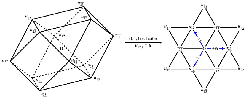
By the (1,1,1)111(1,1,1)-reduction, each cuboctahedron is reduced to a hexagram (see Figure 3.1), which causes the reduction from the face-centred cubic lattice ΩΩ\Omega to the triangle lattice 3/(ϵ1+ϵ2+ϵ3)superscript3subscriptbold-italic-ϵ1subscriptbold-italic-ϵ2subscriptbold-italic-ϵ3\mathbb{Z}^{3}/(\bm{\epsilon}_{1}+\bm{\epsilon}_{2}+\bm{\epsilon}_{3}).

Refer to caption
Figure 3.1. The (1,1,1)111(1,1,1)-reduction of the cuboctahedron.
Lemma 3.3.

The reduced system (3.1) is equivalent to equations the system (2.16).

Proof.

The statement follows from the following correspondences:

bl1,l2(1)=α12,bl2,l3(2)=α23,bl1,l3(0)=α31,d12=δ1,d23=δ2,d13=δ3,formulae-sequencesubscriptsuperscript𝑏1subscript𝑙1subscript𝑙2subscript𝛼12formulae-sequencesubscriptsuperscript𝑏2subscript𝑙2subscript𝑙3subscript𝛼23formulae-sequencesubscriptsuperscript𝑏0subscript𝑙1subscript𝑙3subscript𝛼31formulae-sequencesubscript𝑑12subscript𝛿1formulae-sequencesubscript𝑑23subscript𝛿2subscript𝑑13subscript𝛿3\displaystyle b^{(1)}_{l_{1},l_{2}}=\alpha_{12},\quad b^{(2)}_{l_{2},l_{3}}=\alpha_{23},\quad b^{(0)}_{l_{1},l_{3}}=\alpha_{31},\quad d_{12}=\delta_{1},\quad d_{23}=\delta_{2},\quad d_{13}=\delta_{3}, (3.2a)
ul1,l2,l3=u(l1ϵ1+l2ϵ2+l3ϵ3).subscript𝑢subscript𝑙1subscript𝑙2subscript𝑙3𝑢subscript𝑙1subscriptbold-italic-ϵ1subscript𝑙2subscriptbold-italic-ϵ2subscript𝑙3subscriptbold-italic-ϵ3\displaystyle u_{l_{1},l_{2},l_{3}}=u(l_{1}\bm{\epsilon}_{1}+l_{2}\bm{\epsilon}_{2}+l_{3}\bm{\epsilon}_{3}). (3.2b)

Remark 3.4.

Lemma 3.3 means that the reduced system (3.1) can be obtained from the theory of the τ𝜏\tau-function associated with A2(1)superscriptsubscript𝐴21A_{2}^{(1)\ast}-type discrete Painlevé equations.

We are now ready to prove Theorem 1.1. The (1,1,1)111(1,1,1)-periodic reduction from the system (1.2) to the system (3.1) given in Lemma 3.1, the relation between the system (3.1) and the system (2.16) given in Lemma 3.3, and that between the system (2.16) and the A2(1)superscriptsubscript𝐴21A_{2}^{(1)\ast}-type discrete Painlevé equations (1.4) given in §2.2 and §2.3 collectively give the proof of Theorem 1.1.

4. Concluding remarks

In this paper, we considered a reduction of a system of PΔΔ\DeltaEs, which is unusual in the sense that it has the CACO property but not the widely studied CAC property. We showed how the system (1.2) can be reduced to the A2(1)superscriptsubscript𝐴21A_{2}^{(1)\ast}-type discrete Painlevé equations (1.4) using the affine Weyl group associated with the discrete Painlevé equations.

In a forthcoming paper (N. Joshi and N. Nakazono), we will show how another system of PΔΔ\DeltaEs, which also has the CACO property, can be reduced to the A2(1)superscriptsubscript𝐴21A_{2}^{(1)}-type discrete Painlevé equations (see Table 1.1 for the distinction between A2(1)superscriptsubscript𝐴21A_{2}^{(1)} and A2(1)superscriptsubscript𝐴21A_{2}^{(1)\ast}).

Acknowledgment

N. Nakazono would like to thank Profs M. Noumi, Y. Ohta and Y. Yamada for inspiring and fruitful discussions. This research was supported by an Australian Laureate Fellowship # FL120100094 and grant # DP160101728 from the Australian Research Council and JSPS KAKENHI Grant Numbers JP19K14559 and JP17J00092.

Appendix A Consistency around a cuboctahedron property

In this appendix, we recall the definition of consistency around a cuboctahedron. To define it, we also introduce an additional important property called consistency around an octahedron. We refer the reader to [10] for detailed information about these properties.

A.1. Consistency around an octahedron property

In this subsection, we give a definition of a consistency around an octahedron.

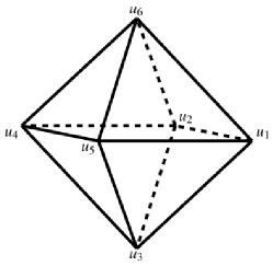
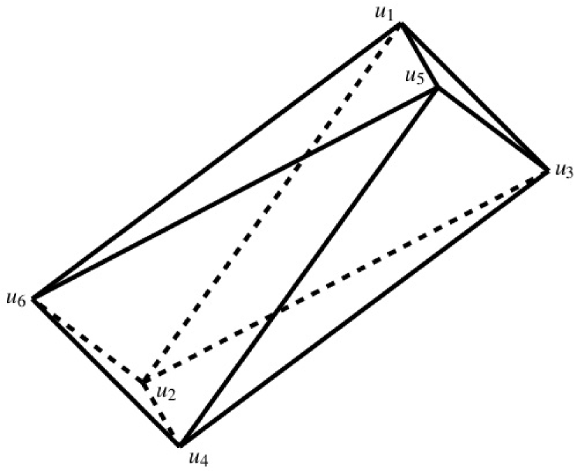
Let uisubscript𝑢𝑖u_{i}, i=1,,6𝑖16i=1,\dots,6, be variables and consider the octahedron shown in Figure A.1. The planes that pass through the vertices {u4,u2,u1,u5}subscript𝑢4subscript𝑢2subscript𝑢1subscript𝑢5\{u_{4},u_{2},u_{1},u_{5}\}, {u2,u6,u5,u3}subscript𝑢2subscript𝑢6subscript𝑢5subscript𝑢3\{u_{2},u_{6},u_{5},u_{3}\} and {u6,u4,u3,u1}subscript𝑢6subscript𝑢4subscript𝑢3subscript𝑢1\{u_{6},u_{4},u_{3},u_{1}\} give 3 quadrilaterals that lie in the interior of the octahedron and we assign the quad-equations Qisubscript𝑄𝑖Q_{i}, i=1,2,3𝑖123i=1,2,3, to the quadrilaterals as the following:

Q1(u4,u2,u1,u5)=0,Q2(u2,u6,u5,u3)=0,Q3(u6,u4,u3,u1)=0.formulae-sequencesubscript𝑄1subscript𝑢4subscript𝑢2subscript𝑢1subscript𝑢50formulae-sequencesubscript𝑄2subscript𝑢2subscript𝑢6subscript𝑢5subscript𝑢30subscript𝑄3subscript𝑢6subscript𝑢4subscript𝑢3subscript𝑢10Q_{1}\left(u_{4},u_{2},u_{1},u_{5}\right)=0,\quad Q_{2}\left(u_{2},u_{6},u_{5},u_{3}\right)=0,\quad Q_{3}\left(u_{6},u_{4},u_{3},u_{1}\right)=0. (A.1)

The consistency around an octahedron property is defined by the following.
Refer to caption
Figure A.1. An octahedron labelled with vertices uisubscript𝑢𝑖u_{i}, i=1,,6𝑖16i=1,\dots,6.
Definition A.1 (CAO property[10]).

The octahedron with quad-equations {Q1,Q2,Q3}subscript𝑄1subscript𝑄2subscript𝑄3\{Q_{1},Q_{2},Q_{3}\} is said to have a consistency around an octahedron (CAO) property, if each quad-equation can be obtained from the other two equations. An octahedron is said to be a CAO octahedron, if it has the CAO property.

A.2. Consistency around a cuboctahedron property

In this subsection, we give a definition of a consistency around a cuboctahedron.

We consider the cuboctahedron centered around the origin whose twelve vertices are given by V={±ϵi±ϵj|i,j,1i<j3}𝑉conditional-setplus-or-minusplus-or-minussubscriptbold-italic-ϵ𝑖subscriptbold-italic-ϵ𝑗formulae-sequence𝑖𝑗1𝑖𝑗3V=\left\{\left.\pm\bm{\epsilon}_{i}\pm\bm{\epsilon}_{j}~{}\right|~{}i,j\in\mathbb{Z},~{}1\leq i<j\leq 3\right\}, where {ϵ1,ϵ2,ϵ3}subscriptbold-italic-ϵ1subscriptbold-italic-ϵ2subscriptbold-italic-ϵ3\{\bm{\epsilon}_{1},\bm{\epsilon}_{2},\bm{\epsilon}_{3}\} form the standard basis of 3superscript3\mathbb{R}^{3}. We assign the variables u(𝒍)𝑢𝒍u({\bm{l}}) to the vertices 𝒍V𝒍𝑉{\bm{l}}\in V and impose the following relations:

Q1(u5,u1,v5,v4)=0,Q2(v2,v1,u2,u4)=0,Q3(u3,u5,v3,v2)=0,formulae-sequencesubscript𝑄1subscript𝑢5subscript𝑢1subscript𝑣5subscript𝑣40formulae-sequencesubscript𝑄2subscript𝑣2subscript𝑣1subscript𝑢2subscript𝑢40subscript𝑄3subscript𝑢3subscript𝑢5subscript𝑣3subscript𝑣20\displaystyle Q_{1}\left(u_{5},u_{1},v_{5},v_{4}\right)=0,\quad Q_{2}\left(v_{2},v_{1},u_{2},u_{4}\right)=0,\quad Q_{3}\left(u_{3},u_{5},v_{3},v_{2}\right)=0, (A.2a)
Q4(v6,v5,u6,u2)=0,Q5(u1,u3,v1,v6)=0,Q6(v4,v3,u4,u6)=0,formulae-sequencesubscript𝑄4subscript𝑣6subscript𝑣5subscript𝑢6subscript𝑢20formulae-sequencesubscript𝑄5subscript𝑢1subscript𝑢3subscript𝑣1subscript𝑣60subscript𝑄6subscript𝑣4subscript𝑣3subscript𝑢4subscript𝑢60\displaystyle Q_{4}\left(v_{6},v_{5},u_{6},u_{2}\right)=0,\quad Q_{5}\left(u_{1},u_{3},v_{1},v_{6}\right)=0,\quad Q_{6}\left(v_{4},v_{3},u_{4},u_{6}\right)=0, (A.2b)
Q7(u4,u2,u1,u5)=0,Q8(u2,u6,u5,u3)=0,Q9(u6,u4,u3,u1)=0,formulae-sequencesubscript𝑄7subscript𝑢4subscript𝑢2subscript𝑢1subscript𝑢50formulae-sequencesubscript𝑄8subscript𝑢2subscript𝑢6subscript𝑢5subscript𝑢30subscript𝑄9subscript𝑢6subscript𝑢4subscript𝑢3subscript𝑢10\displaystyle Q_{7}\left(u_{4},u_{2},u_{1},u_{5}\right)=0,\quad Q_{8}\left(u_{2},u_{6},u_{5},u_{3}\right)=0,\quad Q_{9}\left(u_{6},u_{4},u_{3},u_{1}\right)=0, (A.2c)

where Qisubscript𝑄𝑖Q_{i}, i=1,,9𝑖19i=1,\dots,9, are quad-equations and

u1=u(ϵ2+ϵ3),subscript𝑢1𝑢subscriptbold-italic-ϵ2subscriptbold-italic-ϵ3\displaystyle u_{1}=u(\bm{\epsilon}_{2}+\bm{\epsilon}_{3}), u2=u(ϵ1ϵ3),subscript𝑢2𝑢subscriptbold-italic-ϵ1subscriptbold-italic-ϵ3\displaystyle u_{2}=u(-\bm{\epsilon}_{1}-\bm{\epsilon}_{3}), u3=u(ϵ1+ϵ2),subscript𝑢3𝑢subscriptbold-italic-ϵ1subscriptbold-italic-ϵ2\displaystyle u_{3}=u(\bm{\epsilon}_{1}+\bm{\epsilon}_{2}), u4=u(ϵ2ϵ3),subscript𝑢4𝑢subscriptbold-italic-ϵ2subscriptbold-italic-ϵ3\displaystyle u_{4}=u(-\bm{\epsilon}_{2}-\bm{\epsilon}_{3}), (A.3a)
u5=u(ϵ1+ϵ3),subscript𝑢5𝑢subscriptbold-italic-ϵ1subscriptbold-italic-ϵ3\displaystyle u_{5}=u(\bm{\epsilon}_{1}+\bm{\epsilon}_{3}), u6=u(ϵ1ϵ2),subscript𝑢6𝑢subscriptbold-italic-ϵ1subscriptbold-italic-ϵ2\displaystyle u_{6}=u(-\bm{\epsilon}_{1}-\bm{\epsilon}_{2}), v1=u(ϵ2ϵ3),subscript𝑣1𝑢subscriptbold-italic-ϵ2subscriptbold-italic-ϵ3\displaystyle v_{1}=u(\bm{\epsilon}_{2}-\bm{\epsilon}_{3}), v2=u(ϵ1ϵ3),subscript𝑣2𝑢subscriptbold-italic-ϵ1subscriptbold-italic-ϵ3\displaystyle v_{2}=u(\bm{\epsilon}_{1}-\bm{\epsilon}_{3}), (A.3b)
v3=u(ϵ1ϵ2),subscript𝑣3𝑢subscriptbold-italic-ϵ1subscriptbold-italic-ϵ2\displaystyle v_{3}=u(\bm{\epsilon}_{1}-\bm{\epsilon}_{2}), v4=u(ϵ2+ϵ3),subscript𝑣4𝑢subscriptbold-italic-ϵ2subscriptbold-italic-ϵ3\displaystyle v_{4}=u(-\bm{\epsilon}_{2}+\bm{\epsilon}_{3}), v5=u(ϵ1+ϵ3),subscript𝑣5𝑢subscriptbold-italic-ϵ1subscriptbold-italic-ϵ3\displaystyle v_{5}=u(-\bm{\epsilon}_{1}+\bm{\epsilon}_{3}), v6=u(ϵ1+ϵ2).subscript𝑣6𝑢subscriptbold-italic-ϵ1subscriptbold-italic-ϵ2\displaystyle v_{6}=u(-\bm{\epsilon}_{1}+\bm{\epsilon}_{2}). (A.3c)

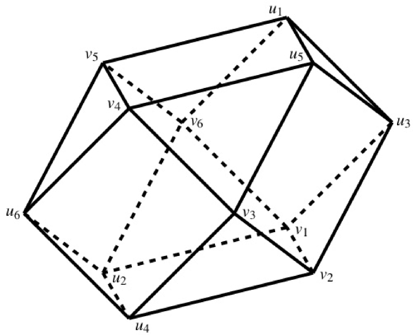
Note that quad-equations Qisubscript𝑄𝑖Q_{i}, i=1,,6𝑖16i=1,\dots,6, are assigned to the faces of the cuboctahedron (see Figure 2(a)). Moreover, uisubscript𝑢𝑖u_{i}, i=1,,6𝑖16i=1,\dots,6, collectively form the vertices of an octahedron and quad-equations Qisubscript𝑄𝑖Q_{i}, i=7,8,9𝑖789i=7,8,9, are assigned to the quadrilaterals that appear as sections passing through four vertices of the octahedron (see Figure 2(b)).
Refer to caption
(a) A cuboctahedron labelled with vertices uisubscript𝑢𝑖u_{i} and vjsubscript𝑣𝑗v_{j}, i,j=1,,6formulae-sequence𝑖𝑗16i,j=1,\dots,6.
Refer to caption
(b) An octahedron labelled with vertices uisubscript𝑢𝑖u_{i}, i=1,,6𝑖16i=1,\dots,6.
Figure A.2. A cuboctahedron and an interior octahedron.

We are now in a position to give the following definitions.

Definition A.2 (CACO property[10]).

The cuboctahedron with quad-equations {Q1,,Q9}subscript𝑄1subscript𝑄9\{Q_{1},\dots,Q_{9}\} is said to have a consistency around a cuboctahedron (CACO) property, if the following properties hold.

(i):

The octahedron with quad-equations {Q7,Q8,Q9}subscript𝑄7subscript𝑄8subscript𝑄9\{Q_{7},Q_{8},Q_{9}\} has the CAO property.

(ii):

Assume that u1,,u6subscript𝑢1subscript𝑢6u_{1},\dots,u_{6} are given so as to satisfy Qi=0subscript𝑄𝑖0Q_{i}=0, i=7,8,9𝑖789i=7,8,9, and, in addition, vksubscript𝑣𝑘v_{k} is given, for some k{1,,6}𝑘16k\in\{1,\dots,6\}. Then, quad-equations Qisubscript𝑄𝑖Q_{i}, i=1,6𝑖16i=1\dots,6, determine the variables vjsubscript𝑣𝑗v_{j}, j{1,,6}\{k}𝑗\16𝑘j\in\{1,\dots,6\}\backslash\{k\}, uniquely.

A cuboctahedron is said to be a CACO cuboctahedron, if it has the CACO property.

Definition A.3 (Square property[10]).

The CACO cuboctahedron with quad-equations {Q1,,Q9}subscript𝑄1subscript𝑄9\{Q_{1},\dots,Q_{9}\} is said to have a square property, if there exist polynomials Ki=Ki(x,y,z,w)subscript𝐾𝑖subscript𝐾𝑖𝑥𝑦𝑧𝑤K_{i}=K_{i}(x,y,z,w), i=1,2,3𝑖123i=1,2,3, where degxKi=degwKi=1subscriptdegree𝑥subscript𝐾𝑖subscriptdegree𝑤subscript𝐾𝑖1\deg_{x}{K_{i}}=\deg_{w}{K_{i}}=1 and 1degyKi,degzKi1subscriptdegree𝑦subscript𝐾𝑖subscriptdegree𝑧subscript𝐾𝑖1\leq\deg_{y}{K_{i}},\,\deg_{z}{K_{i}}, satisfying

K1(v1,u1,u4,v4)=0,K2(v2,u2,u5,v5)=0,K3(v3,u3,u6,v6)=0.formulae-sequencesubscript𝐾1subscript𝑣1subscript𝑢1subscript𝑢4subscript𝑣40formulae-sequencesubscript𝐾2subscript𝑣2subscript𝑢2subscript𝑢5subscript𝑣50subscript𝐾3subscript𝑣3subscript𝑢3subscript𝑢6subscript𝑣60K_{1}(v_{1},u_{1},u_{4},v_{4})=0,\quad K_{2}(v_{2},u_{2},u_{5},v_{5})=0,\quad K_{3}(v_{3},u_{3},u_{6},v_{6})=0. (A.4)

Then, each equation Ki=0subscript𝐾𝑖0K_{i}=0 is called a square equation.

A.3. CACO property of PΔΔ\DeltaEs

We now explain how to associate quad-equations with PΔΔ\DeltaEs in three-dimensional space by using the system of PΔΔ\DeltaEs (1.2) as an example. This requires us to consider overlapping cuboctahedra that lead to two-dimensional tessellations consisting of quadrilaterals. For each given cuboctahedron, there are twelve overlapping cuboctahedra.

The twelve overlapping cuboctahedra around a given one provide six directions of tiling by quadrilaterals. For later convenience, we label directions by ϵi±ϵjplus-or-minussubscriptbold-italic-ϵ𝑖subscriptbold-italic-ϵ𝑗\bm{\epsilon}_{i}\pm\bm{\epsilon}_{j}, 1i<j31𝑖𝑗31\leq i<j\leq 3. Vertices labelled in this way form the set ΩΩ\Omega given by (1.1). Such vertices are interpreted as being iterated on each successive cuboctahedron. We here consider the system of PΔΔ\DeltaEs (1.2). For simplicity, we abbreviate each respective equation in Equations (1.2) as

P1(u13¯,u23¯,u1¯3¯,u2¯3¯)=0,P2(u12¯,u13¯,u1¯2¯,u1¯3¯)=0,P3(u23¯,u12¯,u2¯3¯,u1¯2¯)=0,formulae-sequencesubscript𝑃1subscript𝑢¯13subscript𝑢¯23subscript𝑢¯1¯3subscript𝑢¯2¯30formulae-sequencesubscript𝑃2subscript𝑢¯12subscript𝑢¯13subscript𝑢¯1¯2subscript𝑢¯1¯30subscript𝑃3subscript𝑢¯23subscript𝑢¯12subscript𝑢¯2¯3subscript𝑢¯1¯20\displaystyle P_{1}\left(u_{\overline{13}},u_{\overline{23}},u_{\underline{1}\overline{3}},u_{\underline{2}\overline{3}}\right)=0,~{}P_{2}\left(u_{\overline{12}},u_{\overline{13}},u_{\overline{1}\underline{2}},u_{\overline{1}\underline{3}}\right)=0,~{}P_{3}\left(u_{\overline{23}},u_{\overline{12}},u_{\overline{2}\underline{3}},u_{\underline{1}\overline{2}}\right)=0, (A.5a)
P4(u23¯,u13¯,u23¯,u13¯)=0,P5(u13¯,u12¯,u13¯,u12¯)=0,P6(u12¯,u23¯,u12¯,u23¯)=0.formulae-sequencesubscript𝑃4subscript𝑢¯23subscript𝑢¯13subscript𝑢¯23subscript𝑢¯130formulae-sequencesubscript𝑃5subscript𝑢¯13subscript𝑢¯12subscript𝑢¯13subscript𝑢¯120subscript𝑃6subscript𝑢¯12subscript𝑢¯23subscript𝑢¯12subscript𝑢¯230\displaystyle P_{4}\left(u_{\underline{23}},u_{\underline{13}},u_{\overline{23}},u_{\overline{13}}\right)=0,~{}P_{5}\left(u_{\underline{13}},u_{\underline{12}},u_{\overline{13}},u_{\overline{12}}\right)=0,~{}P_{6}\left(u_{\underline{12}},u_{\underline{23}},u_{\overline{12}},u_{\overline{23}}\right)=0. (A.5b)

Conversely, given 𝒍Ω𝒍Ω{\bm{l}}\in\Omega, we obtain the cuboctahedron centered around 𝒍𝒍{\bm{l}}. We refer to its quad-equations as before by {Q1(𝒍),,Q9(𝒍)}subscript𝑄1𝒍subscript𝑄9𝒍\{Q_{1}({\bm{l}}),\dots,Q_{9}({\bm{l}})\}. Moreover, the overlapped region gives an octahedron centred around 𝒍+ϵ3𝒍subscriptbold-italic-ϵ3{\bm{l}}+\bm{\epsilon}_{3}, and we label its quad-equations by {Q^1(𝒍),Q^2(𝒍),Q^3(𝒍)}subscript^𝑄1𝒍subscript^𝑄2𝒍subscript^𝑄3𝒍\{\hat{Q}_{1}({\bm{l}}),\hat{Q}_{2}({\bm{l}}),\hat{Q}_{3}({\bm{l}})\}.

Each such quad-equation is identified with the 6 partial difference equations given in Equations (1.2) in the following way. For Q1,,Q9subscript𝑄1subscript𝑄9Q_{1},\ldots,Q_{9}, we use

Q1(𝒍)=P1(u13¯,u23¯,u1¯3¯,u2¯3¯)=0,Q2(𝒍)=P1(u1¯3¯,u2¯3¯,u13¯,u23¯)=0,formulae-sequencesubscript𝑄1𝒍subscript𝑃1subscript𝑢¯13subscript𝑢¯23subscript𝑢¯1¯3subscript𝑢¯2¯30subscript𝑄2𝒍subscript𝑃1subscript𝑢¯1¯3subscript𝑢¯2¯3subscript𝑢¯13subscript𝑢¯230\displaystyle Q_{1}({\bm{l}})=P_{1}\left(u_{\overline{13}},u_{\overline{23}},u_{\underline{1}\overline{3}},u_{\underline{2}\overline{3}}\right)=0,\quad Q_{2}({\bm{l}})=P_{1}\left(u_{\overline{1}\underline{3}},u_{\overline{2}\underline{3}},u_{\underline{13}},u_{\underline{23}}\right)=0, (A.6a)
Q3(𝒍)=P2(u12¯,u13¯,u1¯2¯,u1¯3¯)=0,Q4(𝒍)=P2(u1¯2¯,u1¯3¯,u12¯,u13¯)=0,formulae-sequencesubscript𝑄3𝒍subscript𝑃2subscript𝑢¯12subscript𝑢¯13subscript𝑢¯1¯2subscript𝑢¯1¯30subscript𝑄4𝒍subscript𝑃2subscript𝑢¯1¯2subscript𝑢¯1¯3subscript𝑢¯12subscript𝑢¯130\displaystyle Q_{3}({\bm{l}})=P_{2}\left(u_{\overline{12}},u_{\overline{13}},u_{\overline{1}\underline{2}},u_{\overline{1}\underline{3}}\right)=0,\quad Q_{4}({\bm{l}})=P_{2}\left(u_{\underline{1}\overline{2}},u_{\underline{1}\overline{3}},u_{\underline{12}},u_{\underline{13}}\right)=0, (A.6b)
Q5(𝒍)=P3(u23¯,u12¯,u2¯3¯,u1¯2¯)=0,Q6(𝒍)=P3(u2¯3¯,u1¯2¯,u23¯,u12¯)=0,formulae-sequencesubscript𝑄5𝒍subscript𝑃3subscript𝑢¯23subscript𝑢¯12subscript𝑢¯2¯3subscript𝑢¯1¯20subscript𝑄6𝒍subscript𝑃3subscript𝑢¯2¯3subscript𝑢¯1¯2subscript𝑢¯23subscript𝑢¯120\displaystyle Q_{5}({\bm{l}})=P_{3}\left(u_{\overline{23}},u_{\overline{12}},u_{\overline{2}\underline{3}},u_{\underline{1}\overline{2}}\right)=0,\quad Q_{6}({\bm{l}})=P_{3}\left(u_{\underline{2}\overline{3}},u_{\overline{1}\underline{2}},u_{\underline{23}},u_{\underline{12}}\right)=0, (A.6c)
Q7(𝒍)=P4(u23¯,u13¯,u23¯,u13¯)=0,Q8(𝒍)=P5(u13¯,u12¯,u13¯,u12¯)=0,formulae-sequencesubscript𝑄7𝒍subscript𝑃4subscript𝑢¯23subscript𝑢¯13subscript𝑢¯23subscript𝑢¯130subscript𝑄8𝒍subscript𝑃5subscript𝑢¯13subscript𝑢¯12subscript𝑢¯13subscript𝑢¯120\displaystyle Q_{7}({\bm{l}})=P_{4}\left(u_{\underline{23}},u_{\underline{13}},u_{\overline{23}},u_{\overline{13}}\right)=0,\quad Q_{8}({\bm{l}})=P_{5}\left(u_{\underline{13}},u_{\underline{12}},u_{\overline{13}},u_{\overline{12}}\right)=0, (A.6d)
Q9(𝒍)=P6(u12¯,u23¯,u12¯,u23¯)=0,subscript𝑄9𝒍subscript𝑃6subscript𝑢¯12subscript𝑢¯23subscript𝑢¯12subscript𝑢¯230\displaystyle Q_{9}({\bm{l}})=P_{6}\left(u_{\underline{12}},u_{\underline{23}},u_{\overline{12}},u_{\overline{23}}\right)=0, (A.6e)

and for Q^1,Q^2,Q^3subscript^𝑄1subscript^𝑄2subscript^𝑄3\hat{Q}_{1},\hat{Q}_{2},\hat{Q}_{3}, we use

Q^1(𝒍)=P1(u13¯,u23¯,u1¯3¯,u2¯3¯)=0,Q^2(𝒍)=P2(u23¯,u33¯,u2¯3¯,u)=0,formulae-sequencesubscript^𝑄1𝒍subscript𝑃1subscript𝑢¯13subscript𝑢¯23subscript𝑢¯1¯3subscript𝑢¯2¯30subscript^𝑄2𝒍subscript𝑃2subscript𝑢¯23subscript𝑢¯33subscript𝑢¯2¯3𝑢0\displaystyle\hat{Q}_{1}({\bm{l}})=P_{1}\left(u_{\overline{13}},u_{\overline{23}},u_{\underline{1}\overline{3}},u_{\underline{2}\overline{3}}\right)=0,\quad\hat{Q}_{2}({\bm{l}})=P_{2}\left(u_{\overline{23}},u_{\overline{33}},u_{\underline{2}\overline{3}},u\right)=0, (A.7a)
Q^3(𝒍)=P3(u33¯,u13¯,u,u1¯3¯)=0.subscript^𝑄3𝒍subscript𝑃3subscript𝑢¯33subscript𝑢¯13𝑢subscript𝑢¯1¯30\displaystyle\hat{Q}_{3}({\bm{l}})=P_{3}\left(u_{\overline{33}},u_{\overline{13}},u,u_{\underline{1}\overline{3}}\right)=0. (A.7b)

Then, the following proposition holds.

Proposition A.4 ([10]).

The system of PΔΔ\DeltaEs (1.2) has the CACO and square properties, that is, the following statements hold.

(i):

The cuboctahedra with quad-equations {Qi(𝒍)}subscript𝑄𝑖𝒍\{Q_{i}({\bm{l}})\} have the CACO and square properties.

(ii):

The square equations are consistent with the PΔΔ\DeltaEs (1.2).

(iii):

The octahedra with quad-equations {Q^i(𝒍)}subscript^𝑄𝑖𝒍\{\hat{Q}_{i}({\bm{l}})\} have the CAO property.

Appendix B Extended affine Weyl group of type E6(1)superscriptsubscript𝐸61E_{6}^{(1)} and τ𝜏\tau-variables

In this appendix, we review the action of the extended affine Weyl group of type E6(1)superscriptsubscript𝐸61E_{6}^{(1)} given in [23], which is the symmetry group of A2(1)superscriptsubscript𝐴21A_{2}^{(1)\ast}-type discrete Painlevé equations.

Let aisubscript𝑎𝑖a_{i}, i=0,,6𝑖06i=0,\dots,6, be parameters satisfying the condition (2.1) and τj(i)subscriptsuperscript𝜏𝑖𝑗\tau^{(i)}_{j}, i=1,2,3𝑖123i=1,2,3, j=0,1,2,3𝑗0123j=0,1,2,3, be variables. The actions of transformations sisubscript𝑠𝑖s_{i}, i=0,,6𝑖06i=0,\dots,6, and ιjsubscript𝜄𝑗\iota_{j}, j=1,2,3𝑗123j=1,2,3, on the parameters are given by

s0:(a0,a6)(a0,a6+a0),s1:(a1,a2)(a1,a2+a1),:subscript𝑠0maps-tosubscript𝑎0subscript𝑎6subscript𝑎0subscript𝑎6subscript𝑎0subscript𝑠1:maps-tosubscript𝑎1subscript𝑎2subscript𝑎1subscript𝑎2subscript𝑎1\displaystyle s_{0}:(a_{0},a_{6})\mapsto(-a_{0},a_{6}+a_{0}),\qquad s_{1}:(a_{1},a_{2})\mapsto(-a_{1},a_{2}+a_{1}), (B.1a)
s2:(a1,a2,a3)(a1+a2,a2,a3+a2),:subscript𝑠2maps-tosubscript𝑎1subscript𝑎2subscript𝑎3subscript𝑎1subscript𝑎2subscript𝑎2subscript𝑎3subscript𝑎2\displaystyle s_{2}:(a_{1},a_{2},a_{3})\mapsto(a_{1}+a_{2},-a_{2},a_{3}+a_{2}), (B.1b)
s3:(a2,a3,a4,a6)(a2+a3,a3,a4+a3,a6+a3),:subscript𝑠3maps-tosubscript𝑎2subscript𝑎3subscript𝑎4subscript𝑎6subscript𝑎2subscript𝑎3subscript𝑎3subscript𝑎4subscript𝑎3subscript𝑎6subscript𝑎3\displaystyle s_{3}:(a_{2},a_{3},a_{4},a_{6})\mapsto(a_{2}+a_{3},-a_{3},a_{4}+a_{3},a_{6}+a_{3}), (B.1c)
s4:(a3,a4,a5)(a3+a4,a4,a5+a4),s5:(a4,a5)(a4+a5,a5),:subscript𝑠4maps-tosubscript𝑎3subscript𝑎4subscript𝑎5subscript𝑎3subscript𝑎4subscript𝑎4subscript𝑎5subscript𝑎4subscript𝑠5:maps-tosubscript𝑎4subscript𝑎5subscript𝑎4subscript𝑎5subscript𝑎5\displaystyle s_{4}:(a_{3},a_{4},a_{5})\mapsto(a_{3}+a_{4},-a_{4},a_{5}+a_{4}),\qquad s_{5}:(a_{4},a_{5})\mapsto(a_{4}+a_{5},-a_{5}), (B.1d)
s6:(a0,a3,a6)(a0+a6,a3+a6,a6),:subscript𝑠6maps-tosubscript𝑎0subscript𝑎3subscript𝑎6subscript𝑎0subscript𝑎6subscript𝑎3subscript𝑎6subscript𝑎6\displaystyle s_{6}:(a_{0},a_{3},a_{6})\mapsto(a_{0}+a_{6},a_{3}+a_{6},-a_{6}),\qquad (B.1e)
ι1a{0,5,4,6}a{5,0,4,6},ι2a{0,1,2,6}a{1,0,6,2},ι3a{1,5,2,4}a{5,1,4,2},formulae-sequencemaps-tosubscript𝜄1subscript𝑎0546subscript𝑎5046formulae-sequencemaps-tosubscript𝜄2subscript𝑎0126subscript𝑎1062maps-tosubscript𝜄3subscript𝑎1524subscript𝑎5142\displaystyle\iota_{1}a_{\{0,5,4,6\}}\mapsto a_{\{5,0,4,6\}},\quad\iota_{2}a_{\{0,1,2,6\}}\mapsto a_{\{1,0,6,2\}},\quad\iota_{3}a_{\{1,5,2,4\}}\mapsto a_{\{5,1,4,2\}}, (B.1f)

while those on the τ𝜏\tau-variables τj(i)subscriptsuperscript𝜏𝑖𝑗\tau^{(i)}_{j}, i=1,2,3𝑖123i=1,2,3, j=0,1,2,3𝑗0123j=0,1,2,3, are given by

s0subscript𝑠0\displaystyle s_{0} :(τ2(3),τ3(3))(τ3(3),τ2(3)),s1:(τ2(1),τ3(1))(τ3(1),τ2(1)),\displaystyle:(\tau^{(3)}_{2},\tau^{(3)}_{3})\mapsto(\tau^{(3)}_{3},\tau^{(3)}_{2}),\qquad s_{1}:(\tau^{(1)}_{2},\tau^{(1)}_{3})\mapsto(\tau^{(1)}_{3},\tau^{(1)}_{2}), (B.2a)
s2subscript𝑠2\displaystyle s_{2} :(τ1(1),τ2(1))(τ2(1),τ1(1)),:absentmaps-tosubscriptsuperscript𝜏11subscriptsuperscript𝜏12subscriptsuperscript𝜏12subscriptsuperscript𝜏11\displaystyle:(\tau^{(1)}_{1},\tau^{(1)}_{2})\mapsto(\tau^{(1)}_{2},\tau^{(1)}_{1}), (B.2b)
:(τ0(2),τ0(3))((a2+a3)τ1(1)τ0(2)a2τ1(2)τ0(1)a3τ2(1),(a2+a3)τ1(1)τ0(3)a2τ1(3)τ0(1)a3τ2(1)),:absentmaps-tosubscriptsuperscript𝜏20subscriptsuperscript𝜏30subscript𝑎2subscript𝑎3subscriptsuperscript𝜏11subscriptsuperscript𝜏20subscript𝑎2subscriptsuperscript𝜏21subscriptsuperscript𝜏10subscript𝑎3subscriptsuperscript𝜏12subscript𝑎2subscript𝑎3subscriptsuperscript𝜏11subscriptsuperscript𝜏30subscript𝑎2subscriptsuperscript𝜏31subscriptsuperscript𝜏10subscript𝑎3subscriptsuperscript𝜏12\displaystyle:(\tau^{(2)}_{0},\tau^{(3)}_{0})\mapsto\left(\frac{(a_{2}+a_{3})\tau^{(1)}_{1}\tau^{(2)}_{0}-a_{2}\tau^{(2)}_{1}\tau^{(1)}_{0}}{a_{3}\tau^{(1)}_{2}},\frac{(a_{2}+a_{3})\tau^{(1)}_{1}\tau^{(3)}_{0}-a_{2}\tau^{(3)}_{1}\tau^{(1)}_{0}}{a_{3}\tau^{(1)}_{2}}\right), (B.2c)
s3subscript𝑠3\displaystyle s_{3} :(τ1(1),τ1(2),τ1(3),τ0(1),τ0(2),τ0(3))(τ0(1),τ0(2),τ0(3),τ1(1),τ1(2),τ1(3)),:absentmaps-tosubscriptsuperscript𝜏11subscriptsuperscript𝜏21subscriptsuperscript𝜏31subscriptsuperscript𝜏10subscriptsuperscript𝜏20subscriptsuperscript𝜏30subscriptsuperscript𝜏10subscriptsuperscript𝜏20subscriptsuperscript𝜏30subscriptsuperscript𝜏11subscriptsuperscript𝜏21subscriptsuperscript𝜏31\displaystyle:(\tau^{(1)}_{1},\tau^{(2)}_{1},\tau^{(3)}_{1},\tau^{(1)}_{0},\tau^{(2)}_{0},\tau^{(3)}_{0})\mapsto(\tau^{(1)}_{0},\tau^{(2)}_{0},\tau^{(3)}_{0},\tau^{(1)}_{1},\tau^{(2)}_{1},\tau^{(3)}_{1}), (B.2d)
s4subscript𝑠4\displaystyle s_{4} :(τ1(2),τ2(2))(τ2(2),τ1(2)),:absentmaps-tosubscriptsuperscript𝜏21subscriptsuperscript𝜏22subscriptsuperscript𝜏22subscriptsuperscript𝜏21\displaystyle:(\tau^{(2)}_{1},\tau^{(2)}_{2})\mapsto(\tau^{(2)}_{2},\tau^{(2)}_{1}), (B.2e)
:(τ0(1),τ0(3))((a3+a4)τ1(2)τ0(1)a4τ1(1)τ0(2)a3τ2(2),(a3+a4)τ1(2)τ0(3)a4τ1(3)τ0(2)a3τ2(2)),:absentmaps-tosubscriptsuperscript𝜏10subscriptsuperscript𝜏30subscript𝑎3subscript𝑎4subscriptsuperscript𝜏21subscriptsuperscript𝜏10subscript𝑎4subscriptsuperscript𝜏11subscriptsuperscript𝜏20subscript𝑎3subscriptsuperscript𝜏22subscript𝑎3subscript𝑎4subscriptsuperscript𝜏21subscriptsuperscript𝜏30subscript𝑎4subscriptsuperscript𝜏31subscriptsuperscript𝜏20subscript𝑎3subscriptsuperscript𝜏22\displaystyle:(\tau^{(1)}_{0},\tau^{(3)}_{0})\mapsto\left(\frac{(a_{3}+a_{4})\tau^{(2)}_{1}\tau^{(1)}_{0}-a_{4}\tau^{(1)}_{1}\tau^{(2)}_{0}}{a_{3}\tau^{(2)}_{2}},\frac{(a_{3}+a_{4})\tau^{(2)}_{1}\tau^{(3)}_{0}-a_{4}\tau^{(3)}_{1}\tau^{(2)}_{0}}{a_{3}\tau^{(2)}_{2}}\right), (B.2f)
s5subscript𝑠5\displaystyle s_{5} :(τ2(2),τ3(2))(τ3(2),τ2(2)),:absentmaps-tosubscriptsuperscript𝜏22subscriptsuperscript𝜏23subscriptsuperscript𝜏23subscriptsuperscript𝜏22\displaystyle:(\tau^{(2)}_{2},\tau^{(2)}_{3})\mapsto(\tau^{(2)}_{3},\tau^{(2)}_{2}), (B.2g)
s6subscript𝑠6\displaystyle s_{6} :(τ1(3),τ2(3))(τ2(3),τ1(3)),:absentmaps-tosubscriptsuperscript𝜏31subscriptsuperscript𝜏32subscriptsuperscript𝜏32subscriptsuperscript𝜏31\displaystyle:(\tau^{(3)}_{1},\tau^{(3)}_{2})\mapsto(\tau^{(3)}_{2},\tau^{(3)}_{1}), (B.2h)
:(τ0(1),τ0(2))((a3+a6)τ1(3)τ0(1)a6τ1(1)τ0(3)a3τ2(3),(a3+a6)τ1(3)τ0(2)a6τ1(2)τ0(3)a3τ2(3)),:absentmaps-tosubscriptsuperscript𝜏10subscriptsuperscript𝜏20subscript𝑎3subscript𝑎6subscriptsuperscript𝜏31subscriptsuperscript𝜏10subscript𝑎6subscriptsuperscript𝜏11subscriptsuperscript𝜏30subscript𝑎3subscriptsuperscript𝜏32subscript𝑎3subscript𝑎6subscriptsuperscript𝜏31subscriptsuperscript𝜏20subscript𝑎6subscriptsuperscript𝜏21subscriptsuperscript𝜏30subscript𝑎3subscriptsuperscript𝜏32\displaystyle:(\tau^{(1)}_{0},\tau^{(2)}_{0})\mapsto\left(\frac{(a_{3}+a_{6})\tau^{(3)}_{1}\tau^{(1)}_{0}-a_{6}\tau^{(1)}_{1}\tau^{(3)}_{0}}{a_{3}\tau^{(3)}_{2}},\frac{(a_{3}+a_{6})\tau^{(3)}_{1}\tau^{(2)}_{0}-a_{6}\tau^{(2)}_{1}\tau^{(3)}_{0}}{a_{3}\tau^{(3)}_{2}}\right), (B.2i)
ι1subscript𝜄1\displaystyle\iota_{1} :(τj(2),τj(3))(τj(3),τj(2)),ι2:(τj(1),τj(3))(τj(3),τj(1)),\displaystyle:(\tau^{(2)}_{j},\tau^{(3)}_{j})\mapsto(\tau^{(3)}_{j},\tau^{(2)}_{j}),\qquad\iota_{2}:(\tau^{(1)}_{j},\tau^{(3)}_{j})\mapsto(\tau^{(3)}_{j},\tau^{(1)}_{j}), (B.2j)
ι3subscript𝜄3\displaystyle\iota_{3} :(τj(1),τj(2))(τj(2),τj(1)),j=0,1,2,3.:absentformulae-sequencemaps-tosubscriptsuperscript𝜏1𝑗subscriptsuperscript𝜏2𝑗subscriptsuperscript𝜏2𝑗subscriptsuperscript𝜏1𝑗𝑗0123\displaystyle:(\tau^{(1)}_{j},\tau^{(2)}_{j})\mapsto(\tau^{(2)}_{j},\tau^{(1)}_{j}),\qquad j=0,1,2,3. (B.2k)
Remark B.1.
(i):

Each transformation here defined is an isomorphism from the field of rational functions K({τj(i)})𝐾subscriptsuperscript𝜏𝑖𝑗K(\{\tau^{(i)}_{j}\}), where K=({ai})𝐾subscript𝑎𝑖K=\mathbb{C}(\{a_{i}\}), to itself.

(ii):

We follow the convention of Remark 2.1, for Equations (B.1) and (B.2). That is, each transformation acts as an identity on parameters or variables not appearing in its definition.

The transformations collectively form the extended affine Weyl group of type E6(1)superscriptsubscript𝐸61E_{6}^{(1)}, denoted by (2.2). Indeed, the following fundamental relations hold:

(sisj)Aij=1,ι12=ι22=ι32=1,ι1ι2=ι2ι3=ι3ι1,ι2ι1=ι3ι2=ι1ι3,formulae-sequenceformulae-sequencesuperscriptsubscript𝑠𝑖subscript𝑠𝑗subscript𝐴𝑖𝑗1superscriptsubscript𝜄12superscriptsubscript𝜄22superscriptsubscript𝜄321subscript𝜄1subscript𝜄2subscript𝜄2subscript𝜄3subscript𝜄3subscript𝜄1subscript𝜄2subscript𝜄1subscript𝜄3subscript𝜄2subscript𝜄1subscript𝜄3\displaystyle(s_{i}s_{j})^{A_{ij}}=1,\quad{\iota_{1}}^{2}={\iota_{2}}^{2}={\iota_{3}}^{2}=1,\quad\iota_{1}\iota_{2}=\iota_{2}\iota_{3}=\iota_{3}\iota_{1},\quad\iota_{2}\iota_{1}=\iota_{3}\iota_{2}=\iota_{1}\iota_{3}, (B.3a)
ι1s{0,5,4,6}=s{5,0,4,6}ι1,ι2s{0,1,2,6}=s{1,0,6,2}ι2,ι3s{1,5,2,4}=s{5,1,4,2}ι3,formulae-sequencesubscript𝜄1subscript𝑠0546subscript𝑠5046subscript𝜄1formulae-sequencesubscript𝜄2subscript𝑠0126subscript𝑠1062subscript𝜄2subscript𝜄3subscript𝑠1524subscript𝑠5142subscript𝜄3\displaystyle\iota_{1}s_{\{0,5,4,6\}}=s_{\{5,0,4,6\}}\iota_{1},\quad\iota_{2}s_{\{0,1,2,6\}}=s_{\{1,0,6,2\}}\iota_{2},\quad\iota_{3}s_{\{1,5,2,4\}}=s_{\{5,1,4,2\}}\iota_{3}, (B.3b)

where i,j{0,1,,6}𝑖𝑗016i,j\in\{0,1,\dots,6\} and

(Aij)i,j=06=(2000003023000003230000032303000323000003203003002).superscriptsubscriptsubscript𝐴𝑖𝑗𝑖𝑗06matrix2000003023000003230000032303000323000003203003002(A_{ij})_{i,j=0}^{6}=\begin{pmatrix}2&0&0&0&0&0&3\\[-8.00003pt] 0&2&3&0&0&0&0\\[-8.00003pt] 0&3&2&3&0&0&0\\[-8.00003pt] 0&0&3&2&3&0&3\\[-8.00003pt] 0&0&0&3&2&3&0\\[-8.00003pt] 0&0&0&0&3&2&0\\[-8.00003pt] 3&0&0&3&0&0&2\end{pmatrix}. (B.4)
Remark B.2.

The correspondence between the notations in this paper and those in [23] is given by τj(i)τjisubscriptsuperscript𝜏𝑖𝑗subscriptsuperscript𝜏𝑖𝑗\tau^{(i)}_{j}\to\tau^{i}_{j} and τ0(i)s3(τ1i)subscriptsuperscript𝜏𝑖0subscript𝑠3subscriptsuperscript𝜏𝑖1\tau^{(i)}_{0}\to s_{3}(\tau^{i}_{1}), where i,j=1,2,3formulae-sequence𝑖𝑗123i,j=1,2,3.

References

  • [1] V. E. Adler, A. I. Bobenko, and Y. B. Suris. Classification of integrable equations on quad-graphs. The consistency approach. Comm. Math. Phys., 233(3):513–543, 2003.
  • [2] V. E. Adler, A. I. Bobenko, and Y. B. Suris. Discrete nonlinear hyperbolic equations: classification of integrable cases. Funktsional. Anal. i Prilozhen., 43(1):3–21, 2009.
  • [3] R. Boll. Classification of 3D consistent quad-equations. J. Nonlinear Math. Phys., 18(3):337–365, 2011.
  • [4] R. Boll. Corrigendum: Classification of 3D consistent quad-equations. J. Nonlinear Math. Phys., 19(4):1292001, 3, 2012.
  • [5] R. Fuchs. Sur quelques équations différentielles linéaires du second ordre. Comptes Rendus de l’Académie des Sciences Paris, 141(1):555–558, 1905.
  • [6] B. Gambier. Sur les équations différentielles du second ordre et du premier degré dont l’intégrale générale est a points critiques fixes. Acta Math., 33(1):1–55, 1910.
  • [7] B. Grammaticos and A. Ramani. Discrete Painlevé equations: a review. In Discrete integrable systems, volume 644 of Lecture Notes in Phys., pages 245–321. Springer, Berlin, 2004.
  • [8] J. Hietarinta, N. Joshi, and F. W. Nijhoff. Discrete systems and integrability. Cambridge Texts in Applied Mathematics. Cambridge University Press, Cambridge, 2016.
  • [9] R. Hirota. Nonlinear partial difference equations. I. A difference analogue of the Korteweg-de Vries equation. J. Phys. Soc. Japan, 43(4):1424–1433, 1977.
  • [10] N. Joshi and N. Nakazono. Classification of quad-equations on a cuboctahedron. arXiv:1906.06650, 2019.
  • [11] K. Kajiwara. Hypergeometric solutions to the additive discrete Painlevé equations with affine Weyl group symmetry of type E𝐸{E}. Reports of RIAM Symposium, (No.19ME-S2), 2008 (in Japanese).
  • [12] K. Kajiwara, N. Nakazono, and T. Tsuda. Projective reduction of the discrete Painlevé system of type (A2+A1)(1)superscriptsubscript𝐴2subscript𝐴11(A_{2}+A_{1})^{(1)}. Int. Math. Res. Not. IMRN, (4):930–966, 2011.
  • [13] K. Kajiwara, M. Noumi, and Y. Yamada. Geometric aspects of Painlevé equations. J. Phys. A, 50(7):073001, 164, 2017.
  • [14] F. Nijhoff and H. Capel. The discrete Korteweg-de Vries equation. Acta Appl. Math., 39(1-3):133–158, 1995. KdV ’95 (Amsterdam, 1995).
  • [15] F. W. Nijhoff, H. W. Capel, G. L. Wiersma, and G. R. W. Quispel. Bäcklund transformations and three-dimensional lattice equations. Phys. Lett. A, 105(6):267–272, 1984.
  • [16] F. W. Nijhoff, G. R. W. Quispel, and H. W. Capel. Direct linearization of nonlinear difference-difference equations. Phys. Lett. A, 97(4):125–128, 1983.
  • [17] F. W. Nijhoff and A. J. Walker. The discrete and continuous Painlevé VI hierarchy and the Garnier systems. Glasg. Math. J., 43A:109–123, 2001. Integrable systems: linear and nonlinear dynamics (Islay, 1999).
  • [18] J. Nimmo and W. Schief. An integrable discretization of a 2+ 1-dimensional sine-gordon equation. Studies in Applied Mathematics, 100(3):295–309, 1998.
  • [19] P. Painlevé. Sur les équations différentielles du second ordre et d’ordre supérieur dont l’intégrale générale est uniforme. Acta Math., 25(1):1–85, 1902.
  • [20] G. R. W. Quispel, F. W. Nijhoff, H. W. Capel, and J. van der Linden. Linear integral equations and nonlinear difference-difference equations. Phys. A, 125(2-3):344–380, 1984.
  • [21] A. Ramani, B. Grammaticos, and J. Hietarinta. Discrete versions of the Painlevé equations. Phys. Rev. Lett., 67(14):1829–1832, 1991.
  • [22] H. Sakai. Rational surfaces associated with affine root systems and geometry of the Painlevé equations. Comm. Math. Phys., 220(1):165–229, 2001.
  • [23] T. Tsuda. A geometric approach to tau-functions of difference Painlevé equations. Lett. Math. Phys., 85(1):65–78, 2008.