Stellar Masses of Giant Clumps in CANDELS and Simulated Galaxies Using Machine Learning
Abstract
A significant fraction of high redshift star-forming disc galaxies are known to host giant clumps, whose nature and role in galaxy evolution are yet to be understood. In this work we first present a new method based on neural networks to detect clumps in galaxy images. We use this method to detect clumps in the rest-frame optical and UV images of a complete sample of star forming galaxies at in the CANDELS survey as well as in images from the VELA zoom-in cosmological simulations. We show that observational effects have a dramatic impact on the derived clump properties leading to an overestimation of the clump mass up to a factor of 10, which highlights the importance of fair comparisons between observations and simulations and the limitations of current HST data to study the resolved structure of distant galaxies. After correcting for these effects with a mixture density network, we estimate that the clump stellar mass function follows a power-law down to the completeness limit ( solar masses) with the majority of the clumps being less massive than solar masses. This is in better agreement with recent gravitational lensing based measurements. The simulations explored in this work overall reproduce the shape of the observed clump stellar mass function and clumpy fractions when confronted under the same conditions, although they tend to lie in the lower limit of the confidence intervals of the observations. This agreement suggests that most of the observed clumps are formed in-situ.
keywords:
galaxies:evolution - galaxies: formation - galaxies: star formation - galaxies: structure - galaxies: irregular1 Introduction
A prominent feature of distant star-forming galaxies is the frequent presence of high-surface brightness concentrations, or "clumps" embedded in a more uniform light distribution. Their origin and evolution are important to understand many aspects of galaxy formation, e.g., gas accretion, feedback, bulge formation, and supermassive black hole formation. Clumps are mostly identified in rest-frame UV and emission-line (CO or H) images of galaxies over a wide redshift range (e.g., Giavalisco et al., 1996; Conselice et al., 2004; Elmegreen & Elmegreen, 2005; Elmegreen et al., 2007, 2009; Ravindranath et al., 2006; Förster Schreiber et al., 2011; Guo et al., 2012, 2015, 2018; Wuyts et al., 2012; Murata et al., 2014; Shibuya et al., 2016; Soto et al., 2017; Zanella, et al., 2019; Larson et al., 2020; Zick et al., 2020).
Clumps are a few orders of magnitude more massive than star-forming regions in nearby galaxies (e.g., Elmegreen et al., 2007; Genzel et al., 2008, 2011; Förster Schreiber et al., 2011; Guo et al., 2012, 2018; Dessauges-Zavadsky et al., 2017; Soto et al., 2017; Zanella, et al., 2019). Their specific star formation rates are higher than their surrounding areas by a factor of several (e.g., Genzel et al., 2008, 2011; Guo et al., 2012, 2018; Wuyts et al., 2012, 2013; Hemmati et al., 2014; Mieda et al., 2016; Fisher et al., 2017). Their size is still uncertain and under intense debate. Some studies with unlensed galaxies found the size to be 1 kpc (e.g., Elmegreen et al., 2007; Förster Schreiber et al., 2011), but other studies with gravitationally lensed galaxies found smaller sizes of a few hundred or even tens of pc (e.g., Livermore et al., 2012; Zick et al., 2020). Fisher et al. (2017) argue that observation resolution and sensitivity as well as clustering of clumps result in an overestimate of clump sizes. However Cosens et al. (2018) conclude that the size of clumps scales with their H luminosity and there is no difference between lensed and unlensed data.
The formation of clumps is related to the mass assembly processes of galaxies at high redshifts. Clumps are thought to form through gravitational instability in gas-rich turbulent disks, sometimes triggered by external perturbations (e.g., Noguchi, 1999; Immeli et al., 2004a, b; Bournaud et al., 2007, 2009; Elmegreen et al., 2008; Dekel, Sari & Ceverino, 2009; Ceverino et al., 2010, 2012; Dekel & Burkert, 2014; Inoue et al., 2016). This scenario of violent disk instability is supported by some observations, especially for massive clumpy galaxies (e.g., Elmegreen et al., 2007; Bournaud et al., 2008; Genzel et al., 2008, 2011; Guo et al., 2012, 2015; Hinojosa-Goñi et al., 2016; Mieda et al., 2016; Fisher et al., 2017). Clumps, however, can also have an ex-situ origin, that is, as minor mergers (e.g., Hopkins et al., 2013). Evidence of this scenario is also present in the literature (e.g., Puech et al., 2009, 2010; Wuyts et al., 2014; Straughn et al., 2015; Ribeiro et al., 2016). Guo et al. (2015) suggest that the formation mechanisms depend on the mass of clumpy galaxies: clumps in massive galaxies are formed through violent disk instability, while those in lower mass galaxies are formed through minor mergers. If that is the case, one would expect that the clump stellar mass function of clumps changes as a function of galaxy mass.
The evolution of clumps determines their importance on the broad picture of galaxy formation and evolution: whether clumps are building blocks of galactic bulges or just a transient phenomenon. Basically, two scenarios have been proposed. Some models and simulations suggest that clumps can live long enough to migrate towards the centers of their host galaxies, eventually merging into the progenitors of today’s bulges (e.g., Bournaud et al., 2007, 2014; Elmegreen et al., 2008; Ceverino et al., 2010, 2012; Mandelker et al., 2014, 2017). This scenario is supported by observed radial color gradients of clumps (e.g., Förster Schreiber et al., 2011; Guo et al., 2012, 2018; Shibuya et al., 2016; Soto et al., 2017). On the other hand, some other models and simulations suggest that clumps are self-disrupted by their powerful starburst-induced outflows on a timescale of a few tens of Myr (e.g., Murray et al., 2010; Genel et al., 2012; Hopkins et al., 2012, 2014; Buck et al., 2016; Oklopčić et al., 2017). The two scenarios distinguish between different feedback models and strength, i.e., whether the feedback of star formation is strong enough to destroy clumps in a short timescale (e.g., Moody et al., 2014).
An important parameter to understand clump formation and evolution is their stellar mass. For example, as discussed in Dessauges-Zavadsky & Adamo (2018), if clumps were formed in-situ through gravitational instability, the clump mass function would have a slope of (in logarithmic space) at its massive end. The contribution of clump mass to the total mass of their galaxies is also important. Clumps are found to contribute of the total UV luminosity or SFR of their galaxies (e.g., Förster Schreiber et al., 2011; Guo et al., 2012, 2018; Wuyts et al., 2012; Mieda et al., 2016; Rujopakarn et al., 2019), but their contribution to the total stellar mass is still unknown, although it is believed to be small. Clump mass can also be used as a diagnostic of clump evolution. For example, whether the mass of clumps shows any radial variation can be used to test the inward migration scenario (Bournaud et al., 2014). Currently, however, robust measurements of stellar mass for a large sample of clumps are still insufficient in the literature. A challenge of obtaining a complete census of clump mass is to detect clumps in a wavelength that traces stellar mass more than star formation. Rest-frame optical provides a good choice and is accessible by current observing facilities for clumps over a wide range of redshifts.
The capabilities of current observations pose another significant challenge to properly measure physical parameters of clumps. Even with the spatial resolution and sensitivity of HST, clumps at high redshifts can only be marginally resolved or may even be unresolved. Therefore, a clump observed by HST, let alone by ground-based telescopes without Adaptive Optics correction, could be either a single object or the blend of a few nearby smaller clumps. Some authors argued that with a limited spatial resolution of 1 kpc (which is equivalent to HST’s resolution for galaxies at ), many of the giant clumps (with clump stellar mass M⊙) identified in observations are actually the result of blending of smaller structures or clustering of clumps (e.g., Tamburello et al., 2015; Dessauges-Zavadsky et al., 2017; Benincasa et al., 2019; Meng & Gnedin, 2020). Dessauges-Zavadsky et al. (2017) also discuss that the sensitivity threshold used for the clump selection strongly biases against clumps at the low-mass end. Similarly, Fisher et al. (2017) even argue that due to the effects of clump clustering, with a 1 kpc resolution, the SFR surface density of clumps would be overestimated by up to a factor of 20. Some authors (e.g., Buck et al., 2016; Oklopčić et al., 2017) argue that disk stars contaminate clump age measurement, resulting in an artificially old clump age.
In order understand the nature of clumps, a direct comparison between observations and models or simulations is needed. Observational effects related to limited image resolution and sensitivity, such as PSF effects and realistic (and correlated) noises, should be applied to simulations for each specific observation. These forward-modeled simulations have been used in previous studies for integrated galaxies( e.g. Huertas-Company, et al., 2018). For small, faint sub-structures of galaxies, such as clumps, using these forward-modeled simulations is particularly important, because these sub-structures are severely affected by PSF and noise in observations.
In this work we perform several steps towards better quantifying the stellar mass distribution of clumps in distant galaxies. First, we develop a novel method for the detection of clumps based on deep neural networks. The main advantage of this approach is that it is significantly faster and more sensitive than previous methods and therefore can be easily applied to large samples of galaxies in different wavelengths such as the ones that will be soon available (e.g. from JWST, Euclid, and WFIRST). We then apply our method to the five fields of the CANDELS survey (Grogin, et al. 2011; Koekemoer, et al. 2011) in up to seven different detection bands, increasing the sample of clumps by a factor of 3 compared to previous works on the same survey (Guo et al. 2015). More importantly, we statistically quantify for the first time the contribution of clumps to the galaxy stellar mass in a complete sample. We will use state-of-the art cosmological simulations forward modeled in the CANDELS observational plane, namely the VELA hydrodynamic zoom-in simulations (Ceverino et al., 2014), to carry out a direct comparison between observations and simulations of clumps (see also Ginzburg et al. 2020 in prep.). The forward-modeled VELA simulations also help to improve our clump study in two other ways: (1) evaluating the completeness of our sample selection and (2) understanding and correcting systematic and random errors of physical parameter measurements.
The analysis has two main parts: in sections 2 and 3 we present the neural network based clump detector and quantify its accuracy, and in section 4 we apply the new method to a CANDELS subsample of star-forming galaxies and a sample of simulated galaxies, quantify the stellar mases of clumps and discuss clump abundances, clumpy fractions and contribution of clumps to the total galaxy mass in both simulations and observations. Section 5 is a summary and discussion.
Throughout the paper, we adopt a flat cosmology with , and use the Hubble constant in terms of . All magnitudes in the paper are in AB scale (Oke, 1974) unless otherwise noted.
2 Method for clump detections
This section first describes the main method developed in this work to detect clumps.
2.1 Model Architecture
The main purpose of this work is to identify the positions of all off-center clumps belonging to a galaxy in order to characterize their properties. In terms of image processing, the problem can be described as an instance segmentation problem, if one assumes that all clumps have the same geometrical properties. This assumption might not entirely be true. Zanella, et al. (2019) identified for example two populations of clumps with different size distributions. However at first order, clumps are small unresolved sources when compared to the host galaxy.
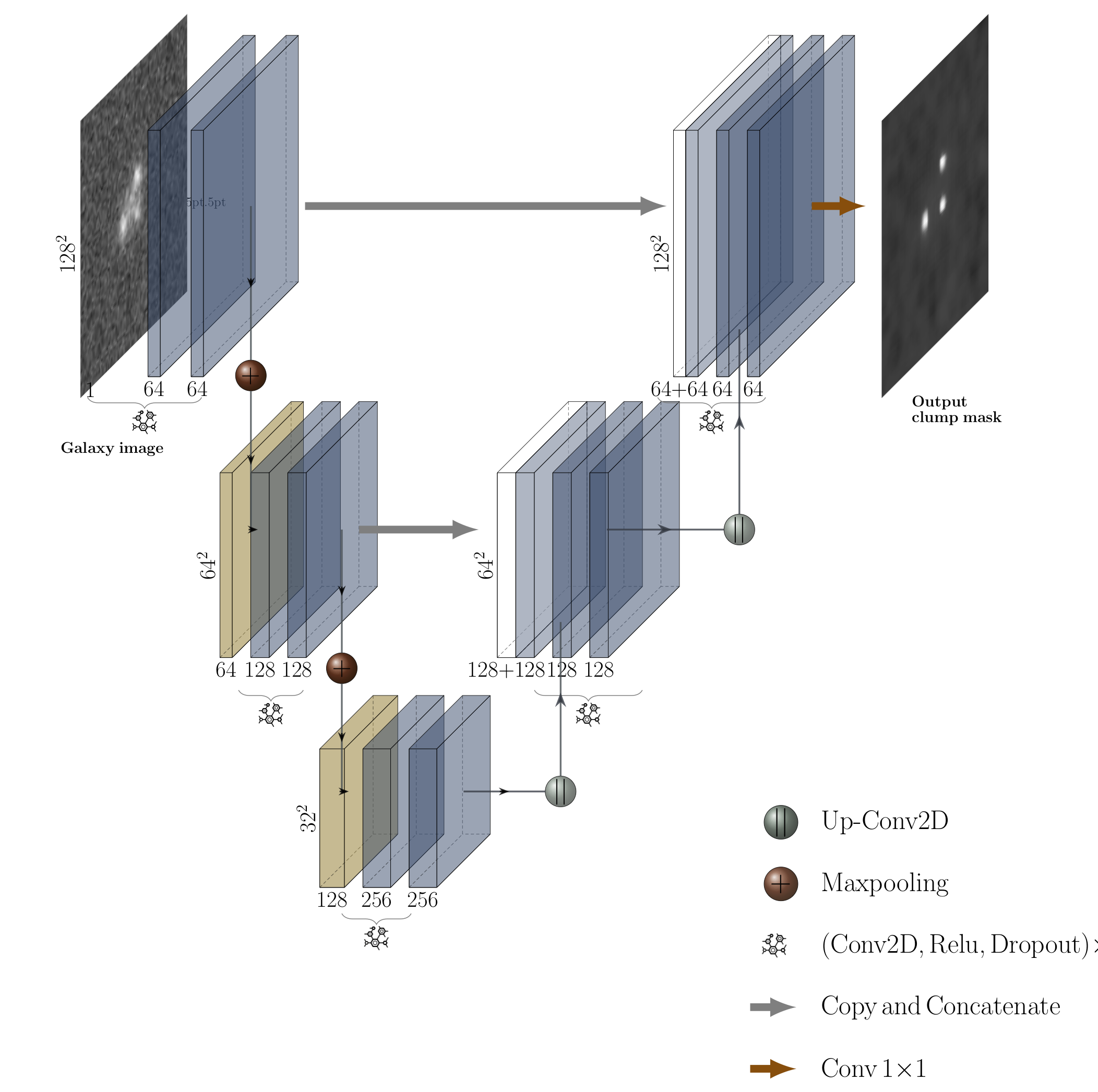
Therefore we decided to use state-of-the-art segmentation networks based on encoder-decoder Convolutional Neural Networks (CNNs). We assume that the detection of the galaxy is done in a previous step. The input for the network is hence a pixels stamp with a galaxy at its center. The desired output is another image with all pixels set to zero except for the pixels belonging to clumps which are set to one. The required configuration is therefore a fully convolutional network whose inputs and outputs are images. We choose here a U-net type architecture (Ronneberger, Fischer & Brox, 2015) that has been proven to be very efficient for image segmentation, especially in the bio-medical field but also in astronomy (e.g. Boucaud, et al., 2020; Hausen & Robertson, 2019)
The encoder part of the network is a standard CNN which takes the image and compresses it to a lower dimension latent space through consecutive convolutions and pooling operations. The decoder part reconstructs an image from the latent space through up-sampling operations. The particularity of the U-net is that there are skipped connections linking the encoder and decoder branches. This has been shown to help in the reconstruction phase and therefore improves the segmentation quality. We use a ReLu activation function in all layers except the last one which is left without activation. We decided to leave the last layer without activation (instead of a Softmax) because it improves the post processing of the detection image to build a clump catalog (see next section). A detailed representation of the specific architecture used in this work is shown in figure 1.
2.2 Simulated training set
The neural network needs to be trained to detect clumps following a supervised approach. To this purpose, a sample of galaxies where the positions of clumps are known is needed. Although there exist catalogs of clumps in observed galaxies from the CANDELS survey, for instance (e.g. Guo et al., 2015, hereafter Guo15), the samples are typically too small for proper training. Furthermore training in real data would propagate any biases existing in the original technique to our clump detector.
We decided then to train the network with simulated galaxies only. We first generate galaxies using a single Sersic analytic profile (Sersic, 1968) using the code GalSim (Rowe, et al., 2015). We allow parameters (e.g total flux, effective radius , Sersic index , axis-ratios ) to vary following uniform random distributions to cover all the observed range from star-forming galaxies in the CANDELS survey (e.g. van der Wel, et al., 2012; Dimauro, et al., 2018). The exact selection of galaxies is described in section 4.
More precisely, we generate galaxies randomly within the following limits: 22 < < 26 (optical bands) and 20 < < 25 (NIR bands); ; ; where n is the galaxy Sersic index, is the semi-major effective radius measured in kpc, and b/a is the axis ratio. To model clumps, we add one or more small sources to each galaxy, generated using GalSim as galaxies with effective radii between 1 and 2 pixels. The number, fluxes, sizes, and positions of clumps are selected randomly, but according to a variety of rules. Generally, we add between 1 and 4 clumps to each galaxy, except for small galaxies () to which we add only 1 or 2 clumps to avoid crowding and to reduce obscuring of the clumps by the galaxy center. For a given galaxy, we limit the combined flux of all clumps to be at most 45% of the total flux (galaxy flux plus clump fluxes). We allow the flux of individual clumps to range from a minimum of 6% to a maximum of 30% of total flux. Finally, we choose clump positions randomly within the annulus 0.5 to 2.0 . For every added clump, we keep in a binary mask the position in the image where it was added. Finally, the image is convolved with a real PSF from the CANDELS survey and noise is added. To model the noise, real empty regions from the CANDELS fields are used in order to include existing spatial correlations.
The procedure is the result of an iterative manual search to come up with a configuration that produces the best results on real data. In particular, we realized that simulating too faint clumps or galaxies without clumps reduces the performance, even if fainter clumps and clump-free galaxies do exist in the observations. In any case, the above procedure should not be considered as unique, and other simulated samples can also produce accurate results.
The above procedure is repeated for seven different filters, four in HST/ACS optical and three HST/WFC3 infrared: (b band), (v band), (i band), (z band), (Y band), (J band) and (H band) using the corresponding noises and PSFs.
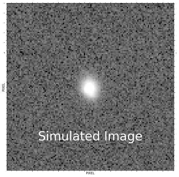
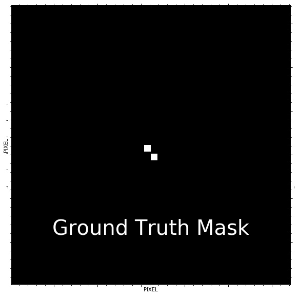
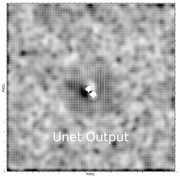
The top row of figure 2 shows an example of a simulated galaxy in the v band with two clumps together with the final mask. Our goal is thus to train the network to predict the mask (top right panel in the figure) given the image of the galaxy (top left panel). Notice that the clumps are barely visible in the image.

2.3 Training and detection procedure
With the training set, we proceed to train the U-net. We train seven different models for the seven different detection bands independently ( (b), (v), (i) ( for COSMOS, EGS and UDS where is not available), (z, for GOODS-N and GOODS-S), (Y), (J) and (H)). In all seven cases, we use a sample of 98,000 galaxies for training while 2,000 galaxies are kept for testing and evaluating the accuracy (see section 2.4). The network is trained following a standard procedure. We use a weighted binary cross-entropy loss to account for imbalance in the training set (the number of pixels belonging to clumps is much smaller than the number of pixels outside clumps) and an Adam optimizer. The initial learning rate is set to and decreased two times by a factor of ten to ease convergence.
As described in the previous section, the output of the network is simply an image with values roughly ranging from 0 to 1. Zero means that no clump is detected at that position, and one means that a clump is detected with high confidence. The output of the U-net needs to be post-processed to decide whether there is a clump or not and also to determine the position of the clump.
To do so, we use SExtractor (Bertin & Arnouts, 1996) on the detection image as a tool to only identify the positions of the detected clumps in each stamp. We emphasize that SExtractor is only used here to identify the centroids of the detected clumps by the neural network. Any other labeling method could have been used at this stage. This allows us to build a catalog containing the positions of all clumps in the stamp. The bottom panels of figure 2 illustrate an example of the prediction steps for one galaxy with two simulated clumps.
2.4 Accuracy of clump detections and flux measurements
We then quantify the accuracy of our clump detector with a set of 2000 galaxies not used for training.
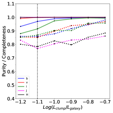
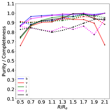
Figure 3 shows first the completeness and purity of the detection as a function of the relative clump luminosity (top) and the clump distance to the galaxy center (bottom) for five photometric bands. Completeness is defined as the fraction of simulated clumps that are detected. Purity measures the fraction of true clumps among all the detected clumps by the U-net. Generally speaking, the figure shows that completeness is overall above in the observed optical bands and slightly lower () in the infrared bands. This is probably a consequence of the difference in spatial resolution between the two cameras (ACS and WFC3) . Purity is generally above 90-95%. This value should be considered as a best case, since the host galaxies are pure analytic profiles so it is very unlikely that there are artifacts detected as clumps except at the very faint end in which noise fluctuations can be sometimes detected as clumps.
The top panel of figure 3 shows the completeness and purity as a function of relative luminosity which has been used in previous works (e.g. Guo15) to select giant clumps. We define the relative clump luminosity as the ratio between the measured clump luminosity and the galaxy luminosity, i.e. ). Overall, completeness increases for brighter clumps. However, even for the faintest clumps (), completeness remains above () for the ACS (WFC3) clumps.
The bottom panel of figure 3 shows that the accuracy of detections does not significantly depend on the position of the clump within the galaxy except perhaps at the very central parts where the central bulges might be sometimes misidentified as clumps. We also observe a decrease of purity at large galactocentric distances for the v band detections. Since this is only appreciated in one filter it is likely to be a statistical fluctuation.
Besides detection, we require an accurate measurement of fluxes given that one of the main purposes of this work is to derive clump stellar masses via SED fitting. Clump fluxes are determined using a simple aperture photometry on each position with a 4 pixel aperture radius as done in Guo15. The measured flux is background subtracted by removing the best fit Sersic model from the host galaxy. In the case of simulations, since the models are pure analytic profiles with known parameters, the correction is straightforward and the flux coming from the galaxy disc is decently removed. This is not the case for real observations, which will be discussed in section 4. We find that, overall, the clump fluxes are recovered accurately with a scatter of dex, with a small increase in scatter for faint clumps. When several clumps are present, the flux of each clump tends to be overestimated because flux from the neighboring clumps is included. It is worth noticing that the Galsim simulations do not include a realistic distribution of clumps. If anything, the number of bright clumps is overestimated as compared to reality (see section 2.2). It is therefore reasonable to expect that the effect of blending of two bright clumps in the observations is small.
3 Performance of clump detector on real observations
The main goal of this work is to apply the clump detector trained on simplistic analytic simulations to real observed galaxies. Training on simulations is particularly dangerous in machine learning where a perfect match between the training and application datasets is assumed. It is therefore critical to properly assess the performance of our clump detector on real observations before moving to any scientific analysis.
We adopt two different approaches to quantify the reliability of the detections. We first quantify how fake clumps inserted on real observed galaxies are detected. We then compare our results with Guo15 detections on the same observed galaxies.
3.1 Detection of fake clumps on real galaxy images
Following the procedure presented in Guo15, we add fake clumps into a sample of real CANDELS galaxies and measure how well we recover them using the developed method. The procedure to add clumps is fully described in Guo15 and we refer the reader to the aforementioned work for more details. This test is intended to quantify how our U-net based detector behaves when confronted with realistic galaxy morphologies while keeping information on the ground truth. For the sake of clarity, we only show the results of this exercise in the filter (i.e., rest-frame UV for CANDELS galaxies) but similar results are observed in the other bands. We emphasize that such a dataset could not have been used for training since it contains a mix of true clumps and fake clumps, making it difficult for the network to understand why some clumps need to be ignored. Since the same galaxies were analyzed also by Guo15, we can also perform a direct comparison between the two methods on the same sample.
Table 1 shows the statistics of the detections for the Guo15 method and our approach. We show the statistics for all clumps first and then for only the brightest clumps. As it can be seen, our method recovers almost all clumps detected by Guo15 on the same galaxies (only of clumps are detected by Guo15 and not by the deep learning approach). This is an indication that even if trained on simplistic simulations, the neural network model behaves as expected. It detects indeed the same clumps as a more traditional and well tested approach would do. Although this might appear surprising, a possible explanation is that this specific task does not depend on the actual galaxy profile. The network essentially learned to detect unresolved off-center sources independently of the galaxy shape. In addition, the neural network is able to detect a significant number of clumps that were undetected by the Guo15 algorithm. This is especially true when all clumps are considered, irrespective of the relative luminosity. The fraction of clumps detected by the U-net but not detected by Guo15 reaches . It suggests that the clump detector presented in this work is more sensitive than the previous algorithms. But when only bright clumps are considered (rightmost column of table 1), the fraction of clumps undetected by Guo15 drops to .
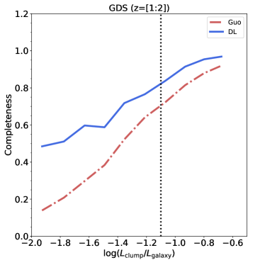
We further quantify the difference in completeness between the two methods in figure 4 which shows the completeness of the detections as a function of the relative clump luminosity. We clearly observe that the DL clump detector has a higher completeness over all the range of clump relative luminosities explored. The difference is particularly pronounced at low relative luminosities which confirms the higher sensitivity of our clump detector. It is particularly interesting that faint clumps are recovered with fairly high completeness even if they were not included in the original simulated training set. In this particular application, using a cleaner training set with only bright clumps, helped the network to generalize. We note also that the values of completeness reported in figure 4 differ slightly from the values reported in figure 3 at similar relative luminosities. This is because the samples are different. One is made only of analytic profiles while the other is composed of real galaxies with fake clumps.
| All | ||
|---|---|---|
| detected in both Guo15 and DL | 51% | 82% |
| detected in Guo15, not detected in DL | 4% | 2% |
| not detected in Guo15, detected in DL | 22% | 10% |
| not detected in Guo15 nor in DL | 23% | 5% |
3.2 Comparison with Guo15
We now perform a direct comparison with the existing real clump detections on galaxies in common with the Guo15 sample. This comparison is more complicated since the ground truth is not known. Therefore, this section is more focussed on exploring the abundances and properties of the clumps detected with both methods to quantify potential differences and biases. We recall that Guo15 only detected clumps in the UV rest-frame bands while with DL we run all bands for all galaxies. The comparison is performed here only for UV rest-frame detections.
We first compare in figure 5 the obtained relative clump Luminosity Functions (cLFs) for different galaxy stellar mass and redshift bins to the one of Guo15 for UV selected clumps ( for and for ). Following Guo15, cLFs are derived by counting the number of clumps in a given relative luminosity bin and dividing by the total number of galaxies in the bin. Guo15 uses only GOODS-S and UDS data. We use here all five CANDELS fields. We see a relatively good agreement between the Guo15 results and ours. Interestingly, the figure also confirms that the deep learning based detector presented here is more complete at low clump relative luminosities. The incompleteness corrected lines from Guo15 indeed better track our raw measurements down to a clump relative luminosity of . However, the uncorrected measurements begin to deviate from the DL sample at a higher relative luminosity threshold. The figure also shows for comparison the cLF of optically detected clumps ( for and for ) which to our knowledge is the first time it is shown. The figure clearly shows that UV rest-frame clumps tend to concentrate a larger fraction of the total galaxy luminosity than optical rest-frame clumps at all redshifts and stellar masses. The abundance of very bright clumps () is around a factor of 10 larger in the UV. This suggests a mild contribution of clumps to the total stellar mass budget that motivates the scientific analysis of the following sections.
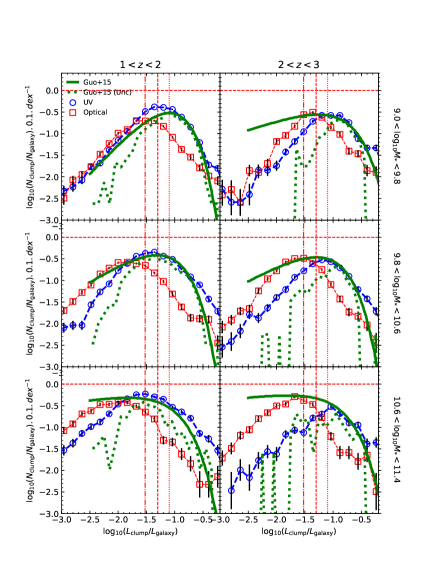
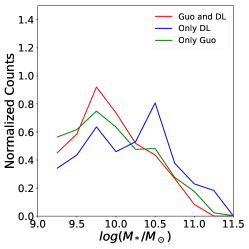
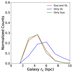
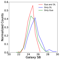
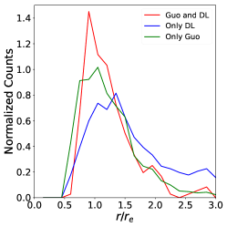
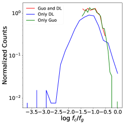
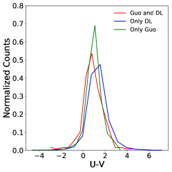
The comparison of figure 5 suggests that the deep learning based detections are more sensitive but recover globally the same population of clumps as the Guo15 algorithm in a given range of clump luminosities. Since clumps are detected in this work with this new method, it is important to properly understand the differences between the populations of clumps detected with both methods before moving to a scientific analysis. To that purpose, we plot in figure 6 some clump and host galaxy properties. We first observe that the DL detections cover essentially the same parameter space as the Guo15 detections. However, they also probe regions in which the Guo15 algorithm detects very few clumps. The clumps not detected by the Guo15 algorithm tend to be at larger galactocentric distances () and in more extended galaxies as revealed by the top panels of figure 6. This again suggests that the DL algorithm is more sensitive and can detect clumps at lower surface brightnesses. As also hinted by the luminosity functions, clumps detected by the DL algorithm in rest frame optical extend to lower relative clump luminosities and such clumps therefore tend to be slightly redder. We note however that in the official Guo15 catalog very faint clumps () have been removed because they are considered unreliable. The DL algorithm also tends to detect a population of bright clumps missed by the Guo15 catalog. A visual inspection reveals that those are bright and large clumps at large distances from the galaxy center. They are most likely minor mergers that the Guo15 algorithm did not select.
Overall, these tests confirm that our clump detector, even if trained only on simplistic simulations, extrapolates surprisingly well to real data and validates its application for a scientific analysis. We emphasize that the goal of this comparison is not to reach a perfect agreement with Guo15 since the approaches are different and both contain misidentifications. The main idea is to verify that there is a reasonable level of agreement between the two approaches which supports the fact that the U-net is behaving well when confronted with real data.
4 Stellar masses of clumps in CANDELS and simulated galaxies
Based on the validation tests presented in the previous sections, we now move to analyze the properties of clumps in the CANDELS survey (Grogin, et al., 2011; Koekemoer, et al., 2011) and in the VELA zoom-in hydrodynamic cosmological simulations (Ceverino et al., 2014; Zolotov et al., 2015) using our deep learning based detector.
4.1 Observational sample
We perform a similar selection to the one done by Guo15 but covering the five CANDELS fields. More precisely, objects are H-band selected () between redshift 0.5 and 3. We then apply additional stellar mass cuts () for completeness reasons. Additionally we include only galaxies with axis ratios larger than 0.5 to avoid highly inclined objects although this also selects agains prolate galaxies (Ceverino et al., 2015; Tomassetti et al., 2016; Zhang, et al., 2019). We exclude very small galaxies ( arscec in the H-band) to avoid spatial resolution related biases. We finally restrict our sample to star-forming galaxies only, defined as objects with Specific Star Formation Rate (sSFR) larger than . All physical quantities are taken from the official CANDELS catalogs (Galametz, et al., 2013; Guo, et al., 2013; Nayyeri, et al., 2017; Stefanon, et al., 2017; Barro, et al., 2019; Santini, et al., 2015). We refer the reader to the mentioned works for details on how these parameters are derived.
We run our seven trained models to detect clumps in seven different bands when available. One of the main purposes of this work is to quantify the distribution of clump masses and their contribution to total galaxy masses. We therefore build a sample of clumps detected in rest-frame optical, which traces older stellar population more effectively than UV. To that purpose, we use detections in the NIR bands: (J) for and (H) for . This selection corresponds roughly to a rest-frame band of nm which should allow to better probe the contribution of clumps to the galaxy stellar mass budget than previous UV based selections. We only consider clumps in the distance range from the galaxy center. The lower limit avoids contamination by the galaxy bulge and the upper limit reduces contaminations from neighboring galaxies.
Although the neural network model is run in all five CANDELS fields and the catalog is released with this work, the following analysis uses data only from the 2 fields (GOODS-S and GOODS-N) that include 7 bands / clump in order to have a better photometric coverage (the other three fields do not have nor coverage). The final sample used for scientific analysis consists of galaxies and detected clumps.
4.2 Simulated sample
We use here the VELA zoom-in hydrodynamic cosmological simulation suite presented and analyzed in a variety of previous works (Ceverino et al., 2014, 2015; Zolotov et al., 2015; Tacchella, et al., 2016a, b; Tomassetti et al., 2016; Huertas-Company, et al., 2018). We refer the reader to the aforementioned works for a detailed description of the simulations. Very briefly, the simulation is made of 35 galaxies simulated with best spatial resolution of 17-35 physical pc and was run with the Adaptive Refinement Tree (ART) code (Kravtsov et al., 1997; Kravtsov, 2003; Ceverino & Klypin, 2009). One important feature for this work is that the high spatial resolution allows tracing the cosmological streams that feed galaxies at high redshift, including mergers and smooth flows, and they resolve the physical phenomena that govern the formation of clumps in the simulation. We stress that full box simulations such as Illustris TNG100 have a typical resolution of kpc (Pillepich, et al., 2018) which prevents properly resolving clump formation. Even the recently completed TNG50 simulation (Pillepich, et al., 2019) does not have enough spatial resolution to resolve the formation of clumps, which requires resolution better than pc. In addition to the high spatial resolution, another advantage of using the VELA simulations is that the properties of clumps are well studied and understood. In Mandelker et al. (2014, 2017) clumps were detected in the VELA galaxies at many timesteps by using both the gas and stellar components in 3D. More details can be found in the aforementioned works.
Following the approach presented in Simons, et al. (2019) and Huertas-Company, et al. (2018), we forward model the 35 galaxies with the radiative transfer code Sunrise111Sunrise is freely available at https://bitbucket.org/lutorm/sunrise. Sunrise images of the VELA simulated galaxies are available online at MAST – see https://archive.stsci.edu/prepds/vela/(Jonsson, 2006; Jonsson & Primack, 2010; Jonsson et al., 2010) and generate HST-like images of galaxies in time steps of Myrs in the redshift range and with the same filters used for the observational sample. We add real noise from the CANDELS survey to the different generated stamps using the procedure outlined in Huertas-Company, et al. (2018). We call the images generated that way VELA Candelized images. The images have been produced using 19 different projections (camera orientations - see Huertas-Company, et al. (2018); Simons, et al. (2019) for details). We use here only cameras 12 to18 which are fully randomly oriented between time steps and are thus independent of the box coordinates and angular momentum. This should indeed be closer to real observations. Additionally, structural parameters are derived for simulated galaxies by fitting Sersic models using GALFIT as for the observations that we use to apply the same selections ( arcsec, ).
4.3 Stellar masses of clumps through SED fitting
Quantifying the contribution of clumps to the galaxy mass requires a proper estimation of the stellar masses of the detected clumps. We use standard SED fitting to estimate the stellar population properties of the clumps in both observed and simulated galaxies.
We first match the optical selected clumps in the six other detection bands. We consider that a clump has been detected in another filter if there is a detection within four pixels of the optical rest-frame detections. Whenever a clump is not detected, we set its flux to 0 in that filter and it is thus not used for the fit. Following this procedure, of the optical detected clumps are detected in at least 3 bands.
We follow the procedure described in section 2.4 for the estimation of clump fluxes. In summary, the clump flux is obtained by performing a 4 pixel aperture photometry at the clump position after removing the flux coming from the disk at the same position and correcting for the PSF aperture. To account for the PSF, we apply a factor of () to the aperture fluxes measured with the ACS (WFC3) cameras. These factors are calibrated by computing the ratio of 4 pixel aperture fluxes over total fluxes in ACS and WFC3 PSFs. The factor is slightly larger for WFC3 because the PSFs are wider. The disk flux is computed by using the best Sersic model for each galaxy in the H-band (van der Wel, et al., 2012 for the observations). Since structural parameters can change with wavelength, we use the multi-wavelength fits to the 2D surface brightness profiles of H-band selected galaxies brighter than published in Dimauro, et al. (2018) to check that using the values derived in the H-band does not significantly change the final clump flux for the brighter galaxies for which we have the structural parameters measured in all wavelengths. Therefore, we assumed that the same will be true for the fainter galaxies and decided to keep the H-band measurements for all galaxies to preserve homogeneity.
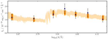
We then perform a fit of the 7 band clump SEDs built as explained in the previous section using the bayesian code Bagpipes (Carnall, et al., 2018). Given the poor photometric coverage of our data, we use a simple tau model for all the clumps with a Calzetti, et al. (2000) dust attenuation law. We use BC03 models (Bruzual & Charlot, 2003) and a Kroupa IMF (Kroupa, 2001). The redshift is fixed at the galaxy spectroscopic redshift when available; if not, the best photometric redshift is used. For the simulations we use the known redshift. We are fully aware that a simplistic tau model is probably not the best SFH model for a clump. We tried an alternative model with constant SFH and the derived stellar masses are essentially the same. As we will discuss in the following sections, a possible route for improvement is the use of non-parametric approaches (e.g. Lower, et al., 2020) but this is for now out of the scope of the present work. The top panel of figure 7 shows an example of the best fit model of an observed clump which has been detected in the 7 photometric bands.
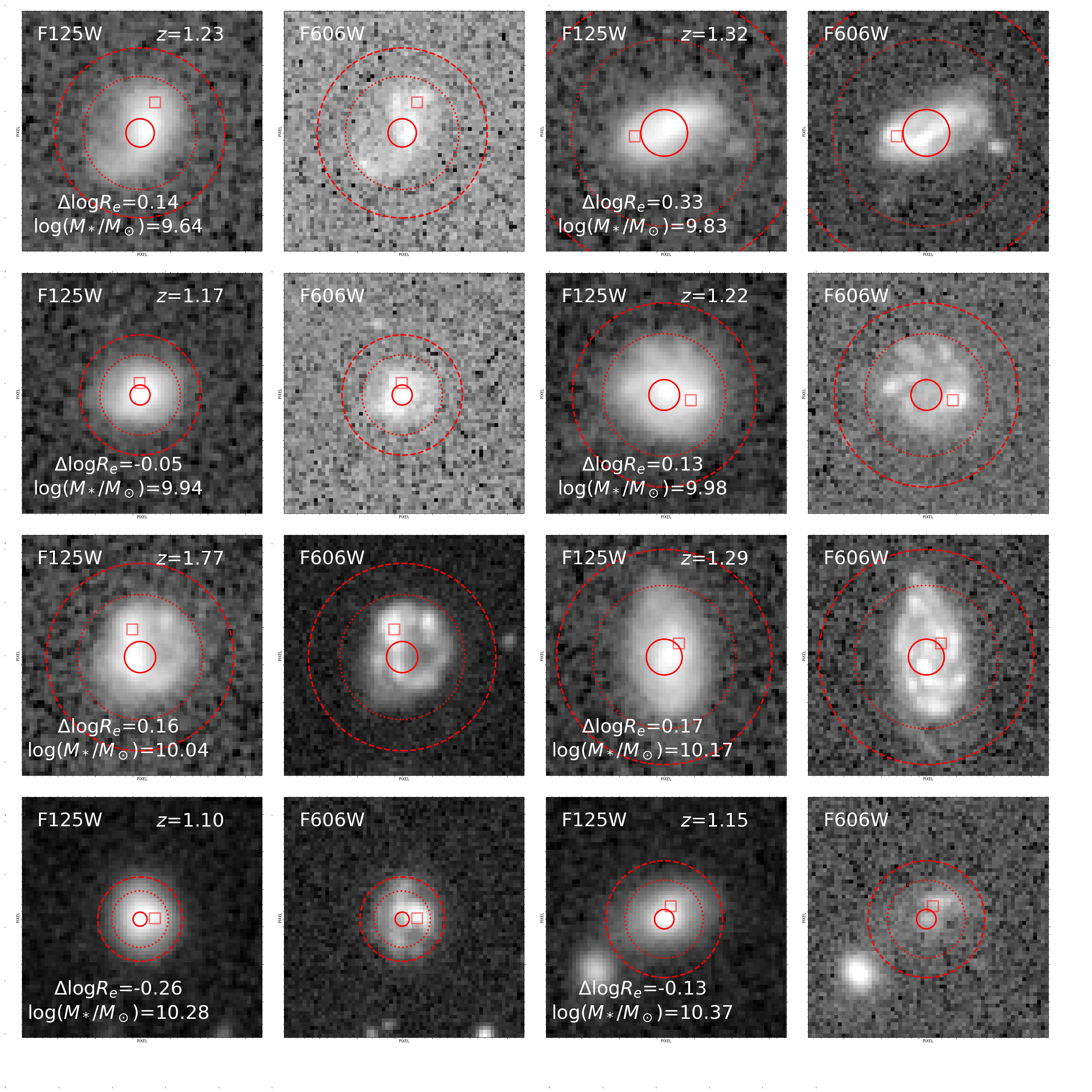
The analysis in the forthcoming sections uses exclusively the stellar mass of the clump. Although the spectral resolution of our data is poor, we find that stellar masses are relatively well constrained by the SED fitting procedure with a typical confidence interval from the posterior distribution of dex. For the cases where fewer than three photometric values are used, the stellar mass uncertainties are around dex. This is certainly high and must be kept in mind when analyzing the results presented in the following sections. Having access to the full posterior enables us to propagate the errors onto the different measurements, as we will discuss as well in the following sections. Figure 8 shows some examples of galaxies with detected massive clumps observed both in the optical and UV rest-frames.
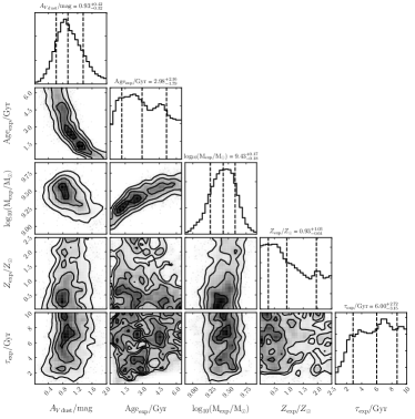
Other quantities such as metallicities and ages are significantly more degenerate, as can be appreciated in the corner plot of figure 7. This is naturally expected from a model constrained with only a few data points. It therefore becomes difficult to use such data for any scientific analysis. Hence we have decided not to discuss clump ages in this work. This will be done in forthcoming dedicated work using an alternative approach (Ginzburg et al. in prep.).
4.4 Impact of observational effects on clump stellar masses and completeness
The comparison with simulations allows us to quantify the impact of observational effects on the derived clump properties from the CANDELS images. Given that the true stellar mass of the clumps is known in the simulation, we can use this as an estimator of the completeness of our deep learning based detector and to assess the accuracy of the clump mass measurements. We use the clumps identified in 3D by Mandelker et al. (2017) as a reference and then match with the 2D detections. Given the much lower resolution of the Candelized images, it is difficult to associate a 2D detection with one unique 3D clump because of blending (see e.g. Moody et al., 2014; Meng & Gnedin, 2020). Therefore, in order to perform the matching between 2D and 3D we follow an alternative approach. We divide the Candelized image in small boxes of pixels ( kpc) and compute the total stellar mass in clumps in the region from the original 3D simulations that falls within each box. We essentially use the clump stellar mass in the catalogs from Mandelker et al. (2017) and add all the clump stellar masses in the pixels region. We then consider that there has been a detection if there is a 2D clump inside the box and associate to the 2D detection the total clump mass computed. We find that of the 2D clumps cannot be associated with a 3D clumps which is consistent with our purity estimations of .
4.4.1 Completeness
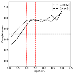
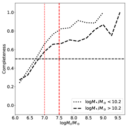
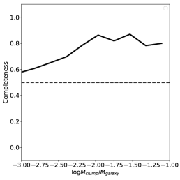
We first quantify the completeness of the detections. Figure 9 plots the fraction of 3D clumps detected in 2D as a function of the the total 3D clump stellar mass in the boxes described previously for two different redshift and galaxy stellar mass bins. The figure also shows the completeness as a function of the ratio between the mass of the clump and the mass of the galaxy. We see that our detector detects of 3D clumps above a stellar mass of solar masses at and that the success rate drops below this mass. At higher redshifts () the completeness starts decreasing at slightly larger masses because galaxies are fainter, but the impact is mild. The dependence with the galaxy stellar mass is more pronounced. Clump detections in massive galaxies are less complete. The reason for this is that the contrast of a clump at fixed mass is weaker in a massive system. This is indeed reflected in the right panel of figure 9. The detections are complete down to a relative clump mass of , which corresponds to different clump stellar masses for massive and low mass galaxies. For simplicity, in the following, we will restrict our analysis to clumps more massive than solar masses. This selection avoids incompleteness related biases on the global population. We shall keep in mind however when interpreting the results that the massive end of the galaxy population might be more affected by incompleteness.
4.4.2 Clump stellar mass accuracy
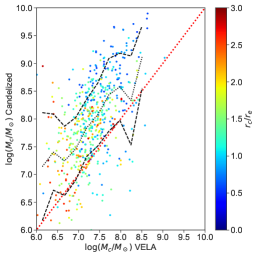
We now look at how well clump stellar masses are recovered from the images using our procedure. We show in the left panel of figure 10 the comparison between the stellar mass for a given 2D detection and the true 3D mass in the associated region (computed by adding up the masses of all 3D clumps projected into the region). Although there is a clear correlation between the true clump masses and the estimated ones, the figure very clearly shows that our SED based method severely overestimates the clump stellar mass by about an order of magnitude. This is true even after adding up all the masses of all clumps in the box. Although surprising, these results are in agreement with previous works which also estimate that the different observational effects can lead to a factor of 10 overestimation of the mass (Meng & Gnedin, 2020; Cava, et al., 2018).
There are several reasons that can explain this big difference. One is obviously spatial resolution, which causes clumps to be blended in the 2D images. We have estimated that each 2D detection corresponds on average to three 3D clumps (see also Moody et al., 2014). Even if this is partially taken into account by adding up the stellar mass of all 3D clumps in a region, blending causes the 2D clump region to also be contaminated by emission from the galaxy which in turn overestimates the mass. The color code of figure 10 shows the distance of each clump to the galaxy center. Clumps for which the stellar mass is most overestimated indeed tend to be in the inner regions where the emission from the galaxy is stronger. This confirms that contamination from the galaxy flux certainly contributes to the overestimation. Another possibility is that the Star Formation Histories (SFHs) adopted to fit the SEDs are not adapted for clumps which are expected to have bursty star formation histories. We recall that we also tried constant SFHs without major changes in the resulting masses. However, the effect of the adopted SFH is something to be investigated in future work by using for example non-parametric SFHs (e.g. Lower, et al., 2020). Overall, these large errors suggest that with current data it is very difficult to establish constraints on individual clump properties. However, it is reasonable to assume that the same biases will be present in the real CANDELS observations. Therefore we can still learn about clump formation by comparing simulations and observations provided they are confronted under comparable conditions, as we will show in the following sections.
4.4.3 Clump stellar mass correction
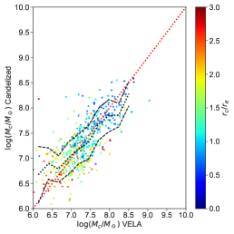
In addition, we can go a step further and use the relation shown in figure 10 to correct the derived stellar masses of the 2D detected clumps if one assumes that the 3D mass is the true mass. The figure shows indeed that there is a correlation between the 3D mass and the estimated mass in 2D with secondary dependences on other parameters such as the clump distance. It should be possible therefore to find a function so that where and are the 3D and 2D clump stellar masses respectively and is a vector containing any other secondary parameters. Since we do not know a priori the analytic form of , we model it with a mixture density network. We define as a 6 dimensional vector containing the clump distance to the center which we have seen correlates with the stellar mass difference, the inclination of the galaxy (), the effective radius of the galaxy () and the Sersic index () derived from the best Sersic fit, the stellar mass of the galaxy and the redshift. We model the posterior distribution with a Gaussian probability density function () and train the neural network to maximize the log likelihood of the true clump mass value. We then use the mean of the posterior distribution to compute the estimated . We train the network using the clump measurements in the simulated images obtained with all random camera projections except one, which is used to test. Since the different projections are fully random, the clump 2D masses and the best fit Sersic parameters of the galaxies can be considered as independent across projections. Once trained, we use the learned model, , to test the correction on the clumps detected on the camera not used for training. The results are shown in the middle panel of figure 10 for camera 15, but similar results are obtained for other camera orientations.
We can easily see that the corrected 2D masses are now in much better agreement with the 3D measurements. This proves that it is possible to recover the intrinsic 3D clump mass (in the box) given the 2D measurement. We note that the correction does not significantly depend on the exact architecture used for the neural network nor on the initialization of it. We tried 50 different random models, including more complex posteriors modeled with a mixture of Gaussians and changing the number or layers and number of units in each layer. This model uncertainty will be incorporated into the error budget in the following sections. We have also tried adding additional parameters to the network such as clumps colors and luminosities without any significant impact.
Although the correlation shown in the middle panel of figure 10 represents a significant improvement compared with the uncorrected values, we notice that the estimator is still biased at the low and high mass ends. As a matter of fact, at the high mass end, the predictions are under estimated and the opposite happens at the low mass end. This is important because it means that the current estimator will tend not to estimate clump masses larger than solar masses which could bias our results when applied to real observations. The reason for this bias is that the posterior distribution estimated by the mixture density network represents in fact the posterior under the training prior . Since the VELA sample used for training contains very few clumps with masses at the edges of the distribution, i.e. larger than and smaller than solar masses, the estimator tends to shift the posterior towards the prior to minimize the risk of failure.
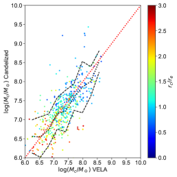
In order to correct for that effect, we attempt to estimate a posterior under a flat prior by renormalizing the posterior distribution under the VELA prior () using the following relation:
Since is a constant, it simply implies dividing the posterior estimated by the density network by the VELA prior. The result of applying the posterior under a flat prior to estimate the clump mass is shown in the right panel of figure 10. We can see that the estimator is now less biased especially at the edges of the distribution. The scatter also tends to increase. This is because the estimated values are no longer pushed towards the average value of the prior distribution which is around solar masses.
In the following sections we will analyze the impact of these different corrections on the derived clump properties in the observations and in the forward modeled simulations.
4.5 Clump Stellar Mass Function
We start our analysis by focusing on the clump stellar mass function (cSMF) which can provide interesting clues about the physical processes governing clump formation. For example, several works have pointed out that the slope of the cSMF might be indicative of the formation mechanisms (e.g. Elmegreen, et al., 2006; Dessauges-Zavadsky & Adamo, 2018; Elmegreen, 2018). If clumps are formed by turbulence driven fragmentation of gas clouds, the resulting slope of the cSMF is expected to be around (Elmegreen, 2018). Also, clumps formed ex-situ are expected to be on average more massive than in-situ formed clumps (Mandelker et al., 2017) so the distribution of clump stellar mass can also provide clues about the origin of the clumps.
4.5.1 Impact of observational effects on the clump stellar mass function
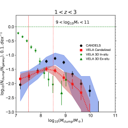
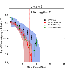
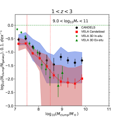
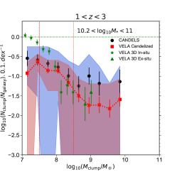
Before analyzing the clump stellar mass function, it is important to first calibrate the amount of information that can be recovered from the CANDELS-like images given the large uncertainties in the clumps stellar masses reported in the previous subsection. To that purpose, we first compare the cSMF derived using the detections performed on the Candelized VELA simulation with the clump stellar mass function obtained using the raw 3D output from the VELA simulations analyzed by Mandelker et al. (2017). This is shown in the left panel of figure 11. The values are normalized by the total amount of galaxies in a given bin. The sample only contains 35 galaxies. However, since images are produced in every time step, using only one camera results in a sample of few hundred images in the redshift range of interest (). For this exercise of building the mass functions, we consider each image as if it was an independent galaxy with a given stellar mass and redshift. Since the galaxy sample is still small, we compute the cSMF for all galaxies together (). The shaded region indicates how the results change depending on the camera orientation used.
First of all, we see a dramatic difference between the cSMF derived with the Candelized images and the true 3D based cSMF. The Candelized cSMF peaks at a clump mass of while the 3D mass function shows a power-law increase at low masses without any flattening as opposed to the observations. This big difference between 3D and 2D cSMFs is expected, given the several systematics that affect the measurements in the Candelized images reported in the previous subsections. One is obviously incompleteness. Because Candelized images are affected by noise, low mass clumps are not detected by our clump detector as already discussed in subsection 4.4. Additionally, clump blending can also contribute to lower the normalization of the cSMF. The HST PSF is kpc in the redshift range of interest which means that on average one HST clump corresponds to three 3D clumps. Although completeness and blending can contribute to change the slope, they are not enough to change the shape of the cSMF so dramatically. A key and dominant effect comes from the systematic errors in the SED based estimations of clump stellar masses shown in figure 10. Both the systematic clump mass overestimation and Eddington bias (Eddington, 1913) will tend to change the shape of the cSMF by over populating the high mass end and decreasing the slope as we seem to see. In appendix A we show indeed that a combination of these effects can reconcile the intrinsic 3D cSMF with the observed one. This suggests that, with current data and no correction, it is difficult to use the shape of the clump stellar mass function as a constraining parameter for clump formation.
The left panel of figure 11 also includes the measurements obtained on observed CANDELS galaxies. Due to the small sample size and the VELA halo masses being roughly uniformly distributed in log mass, the VELA galaxies’ stellar mass distribution is different from that of our CANDELS mass-complete sample. To take that into account for a fair comparison, we create samples from the parent CANDELS sample of equal size as the VELA sample to reproduce the number, stellar mass and redshift distributions of the VELA sample. We call these samples the CANDELS-VELA samples. The cSMF for the CANDELS-VELA samples are plotted in the shaded red regions of figure 11 which provide an estimate of the confidence interval. Although the observational points tend to lie above the simulated ones, an important result is that, overall, the simulated points lie within the confidence interval of the observations. Additionally, the shapes of the cSMFs are very similar. This means that the VELA simulations predict globally the correct number of clumps when compared with observations under comparable conditions. It also means that even if the observed cSMF differs from the true one, the same systematics seem to apply to both observations and simulations when the latter are forward modeled to the observational plane. This clearly demonstrates that it is of capital importance to compare observations and simulations under the same conditions, especially in the low S/N and low resolution regimes. It also highlights the limitations of current HST data to study the resolved structure of high redshift galaxies and the importance of future JWST observations.
4.5.2 Corrected clump stellar mass function
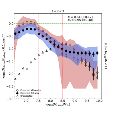
In this work, we go a step further and try to correct the estimated clump stellar masses to recover the intrinsic clump stellar mass function. The middle and right panels of figure 11 show the corrected stellar mass functions using the neural network trained as detailed in section 4.4. We show the results of the two different priors. We clearly see that the corrected observed cSMFs do agree significantly better with the intrinsic 3D mass function. This confirms that the correction applied is effective. In particular, the peak of the cSMF is now shifted to lower masses and the mass function presents a steep decrease between and solar masses. Between and , the impact of the prior applied in the correction is rather small. Most of the differences are seen in the high mass end, where the flat prior correction tends to predict more clumps. The uncertainties are also large. As we have seen, the VELA prior prediction tends to underestimate the number of clumps above solar masses. The flat prior prediction will tend to compensate for the lack of training points on the massive end. By doing so, it will also tend to over estimate the number of massive clumps as the correction boosts the posterior distribution outside the training values. Overall, the exact abundances remain quite uncertain given the lack of training points. However, both corrections should bracket the range of possible values.
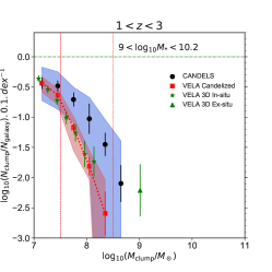
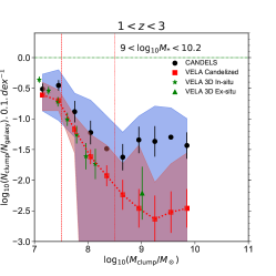
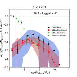
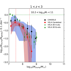
As a way of quantifying how well the intrinsic cSMF can be recovered at least in the range of masses in which the correction is more stable, we also report in table 2 the slopes of the best power law model fits () to the VELA 3D, VELA Candelized and VELA-CANDELS samples after the correction of the stellar masses is applied. We restrict to the mass range where the mass function is better constrained. Although the true 3D clump mass function has a steeper slope than the measured with the corrected values, it is within the confidence intervals of the derived slopes with both the VELA and flat prior. This suggests that the correction enables us to recover to some extent the intrinsic slope and shape of the 3D cSMF. The reason why the recovered slope is still shallower than the intrinsic one might be related to both errors in the correction and also completeness and blending effects. We note however that the relative agreement between CANDELS and VELA is independent of the correction applied as both cSMFs agree even when uncorrected values are used. It is also worth noticing that the slope measured for the 3D cSMF is shallower than the value of (see table 2) even if the clumps are known to be formed in-situ. This is not entirely surprising. The measured slope is expected to be shallower than the birth slope given that clumps of different masses have different lifetimes (Tacchella, Forbes, & Caplar, 2020).
Given that the correction applied seems to allow the recovery of the intrinsic cSMF at least in broad terms, we now move to explore the corrected cSMF using the whole CANDELS dataset. This is of course more risky, as the CANDELS sample necessarily contains more galaxies not well covered by the VELA training set, so the results need to be taken with caution. This is shown in figure 12. We show both the uncorrected and corrected cSMFs with the two different priors. The shaded region in the figure shows the range of solutions obtained using different neural network models and the black points are the average values.
First of all we see that, although there is some range of possible solutions, the global shape of the mass function is consistent across the different neural network models. Overall, the correction has a similar effect on the cSFMs as the one reported for VELA which is reassuring. Namely, the peak of the cSMFs is displaced towards lower masses from to . Overall, the cSMF presents a steep increase with decreasing clump mass until reaching a peak close to the solar masses for corrected masses and starts declining again at lower masses with a shallower slope. The peak of the cSMF is most probably due to incompleteness as it matches reasonably well the value estimated in figure 9 and there is no particular physical reason to expect a flattening at the low mass end.
Another interesting result is that regardless of the correction applied, the majority of the clumps have stellar masses lower than solar masses. The abundances of massive clumps are poorly constrained though, as they depend on the prior used to correct masses. The correction using flat prior tends to estimate large abundances of massive clumps. As previously explained, this is an upper limit, as the correction applied boosts the posterior distribution beyond the training regime. However, the fact that the cSMF tends to peak at masses close to is a robust result that is not significantly affected by the correction applied. This order of magnitude for the typical clump masses is also in better agreement with recent independent measurements of clump masses using gravitational lensing techniques.
4.5.3 Implications for the formation and origin of clumps
Although significantly affected by uncertainties, the derived clump stellar mass function and the comparison with simulations allow us to speculate about the nature of giant clumps in high redshift galaxies.
First of all, our results suggest that the majority of the clumps detected in high redshift galaxies are less massive than solar masses. Although our results do not allow us to put strong constraints on the abundances of very massive clumps, it seems clear that the bulk of the population has lower masses. This is an important assessment, as some previous works have estimated that high redshift clumps are frequently more massive than solar masses (e.g. Förster Schreiber et al., 2011; Zanella, et al., 2019). Our results suggest that these measurements might have been affected by similar systematic biases raised in this work, as pointed out for example in Cava, et al. (2018) using gravitationally lensed data. The different selections can perhaps also explain some of the differences, as the aforementioned works do not analyze complete samples and might have biased their selection towards galaxies with prominent clumps.
Secondly, our results also show that the simulations globally reproduce the shape of the observed cSMF irrespective of any correction applied. This agreement between simulated and observed cSMFs potentially puts some constraints on the origin of clumps detected in the observations. In the VELA simulations, the majority of the clumps are formed in-situ and therefore ex-situ clumps alone could not account for the agreement observed in figure 11. Furthermore, ex-situ clumps are predicted to be significantly more massive than in-situ clumps. This implies that the majority of observed clumps in CANDELS must have an in-situ origin. In order to further assess this, we perform a match of the 2D Candelized clumps with the 3D clumps as done in subsection 4.4 and flag all 2D clumps which correspond to an ex-situ clump in the simulation. We find that only 5 clumps (4 at and 1 at ) among the 186 detected clumps are flagged as ex-situ. This represents of the clumps and has basically no effect in the derived cSMF. Therefore the observed agreement between observations and simulations must be driven by in-situ clumps. This is the first time that evidence of an in-situ origin for most clumps is shown through direct comparison of observations with numerical simulations.
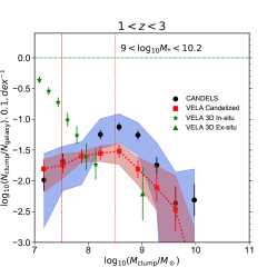
An interesting question related to the clump origin is whether it depends on the galaxy properties such as stellar mass. Given that our results seem to point towards an in-situ origin of clumps, one might wonder if the galaxy properties affect the shape of the cSMF. Although our sample is small, we address this issue in figure 13 where we show the cSMFs for simulated and observed galaxies in two broad galaxy stellar mass bins. The different slope measurements are also reported in table 2. The effect of galaxy stellar mass on the intrinsic 3D cSMF is very mild, suggesting that galaxy stellar mass has little effect on the properties of formed clumps. This is not entirely surprising. The work by Inoue et al. (2016) shows that external events such as minor mergers often trigger the formation of clumps. However, we see that the slopes derived from the 2D Candelized data tend to be shallower in massive galaxies. We argue that this is most likely related to incompleteness. As discussed in section 4.4, lower mass clumps detected in massive galaxies are less complete. This implies a decrease of the cSMF at the low mass end as seen in figure 13, which in turn results in a shallower slope. We do not think it has a physical origin as the effect is not seen in 3D. It illustrates how completeness can affect the measurement of the slope.
| w/ VELA prior | w/ flat prior | |
| VELA in-situ | ||
| VELA Candelized | ||
| CANDELS (VELA sample) | ||
| CANDELS (All sample) | ||
| VELA in-situ | ||
| VELA Candelized | ||
| CANDELS (VELA sample) | ||
| VELA in-situ | ||
| VELA Candelized | ||
| CANDELS (VELA sample) |
4.6 Contribution of clumps to stellar mass
In order to better investigate how the clump abundances depend on different galaxy properties without being affected by small numbers, we adopt a summary statistic which measures the total fraction of stellar mass () contained in clumps. is directly related to the integral of the cSMF and can be estimated by dividing the total clump stellar mass by the total galaxy mass in a given sample. For the sake of clarity we only report results using corrected masses with a flat prior, although the main trends do not change if a VELA prior is used. We therefore set here a lower limit of solar masses for the clumps to avoid incompleteness issues.
4.6.1 Observations
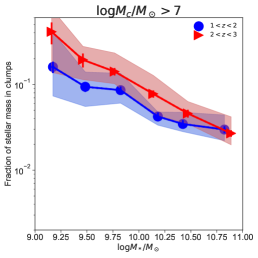
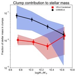
The left panel of figure 14 shows as a function of galaxy stellar mass and redshift for all our CANDELS sample. Error bars are computed by performing MonteCarlo simulations through the sampling of the posteriors of the clump stellar masses. For every iteration we sample the posterior to associate a stellar mass to every clump and recompute . The reported values of are then the median values of the different realizations and the error bars correspond to the standard deviation from the different samples. The shaded regions show the range of values depending on the neural network model used to correct the stellar masses among the 100 realizations. The figure first shows that decreases with increasing galaxy mass. For galaxies more massive than solar masses, clumps contain on average between and of the total stellar mass. The fraction increases for low mass galaxies, reaching although the uncertainties are large. This large uncertainty at low masses is driven by low statistics and the uncertainties regarding the amount of massive clumps reported in the previous section. Higher redshift galaxies tend also to have larger fractions of mass in clumps since the red points in figure 14 are systematically above the blue ones.
The average value of of the stellar mass seems to be smaller than values reported in the literature with smaller samples too. Förster Schreiber et al. (2011) quotes for example fractions of of the galaxy stellar mass in clumps using a sample of 6 galaxies. In the recent work by Zanella, et al. (2019) the authors analyzed star-forming galaxies and found that of the stellar mass is in compact clumps which should be comparable to our selection. There are several reasons why our measurements are smaller. First of all, and most importantly, we are correcting the clump stellar masses for the overestimation reported in section 4.4. This correction primarily reduces the clump stellar masses by an order of magnitude, therefore reducing their contribution to the total galaxy mass. We assume that previous measurements could have suffered from similar overestimations and thus reported larger values. However, even if we use uncorrected clump mass measurements, typically reaches values of which is still smaller than other reported values. Another factor is that our analysis is made on a complete sample of galaxies ( as opposed to a few tens). Our sample thus contains clumpy galaxies but also galaxies which do not host any clump, so the overall stellar mass fraction decreases. Wuyts et al. (2012) measured indeed a value of using both clumpy and non-clumpy galaxies which is in better agreement with our uncorrected measurements. Additionally the Zanella, et al. (2019) sample for example is dominated by galaxies with stellar masses lower than solar masses for which we also measure a larger contribution of clumps (figure 14(a)). Approximately of their sample is made of starbursts which can also boost the obtained stellar mass fractions.
Our mass complete sample allows us to also investigate how the abundance of clumps depends on galaxy properties, which is more difficult with incomplete samples such as the ones usually explored in the previous works. We focus here on effective radius () and specific-star formation rate (sSFR). There are indeed well established scaling relations between stellar mass and size and stellar mass and star-formation rate (the star-formation main sequence) which have been extensively studied (e.g. van der Wel, et al., 2014; Whitaker, et al., 2012) and are thought to be central for describing major evolutionary tracks of galaxies (e.g. Barro, et al., 2014; Rodríguez-Puebla, et al., 2017; Chen, et al., 2019; Lin, et al., 2019). Our goal is to investigate whether clumps can provide clues about the physics of galaxies along these tracks.
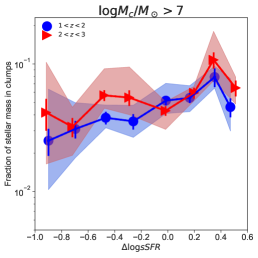
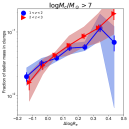
We therefore start by analyzing whether clumps are more likely to be formed in galaxies which deviate from these median scaling relations. We adopt here and as main proxies, which precisely measure how far the specific star formation rate and the effective radius are from the median - and - relations. values have the advantage of taking into account the mass dependence and allow us to explore the average relation without further binning in galaxy stellar mass. We use the best fit relations from Fang, et al. (2018) as reference values for the CANDELS galaxy scaling relations. Positive / negative values of values therefore indicate galaxies above / below the median scaling relation at fixed stellar mass.
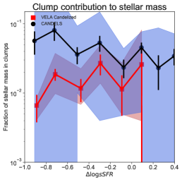
The middle and right panels of figure 14 show the dependence of with and respectively. First we see that there is very little dependence of the clump contribution with the relative position of galaxies in the main sequence. The value of is almost constant, although there is a hint of a slight increasing trend in galaxies with a larger sSFR than the average of the same mass. Since the sSFR is expected to correlate with the gas mass density, one would naturally expect a larger contribution of clumps in galaxies above the main sequence. Several reasons can account for this weak correlation. Errors in both quantities (clump mass fractions and sSFR) can wash out the trend. The difference in the star-formation rates in our sample might not be large enough to notice a strong effect on the clump properties (recall we select only galaxies with ). Some theoretical works (e.g. Inoue et al., 2016) have also shown that clump formation is generally triggered by external perturbations such as minor mergers. This can also contribute to explain the lack of correlation with the main sequence offset. We also note that this weak correlation is independent of the galaxy stellar mass. If the sample is restricted to massive galaxies only we see a similar trend.
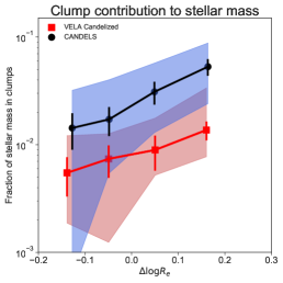
In the right panel of figure 14 we plot the dependence of with . We observe here a clear dependence. Galaxies with larger effective radii than the average in galaxies of the same stellar mass have a higher fraction of their mass in clumps reaching up to at which is three times the value for smaller galaxies. We recall that the stellar mass dependence has been removed. If this increasing trend was driven by different mass distributions, the opposite trend would have been expected, since large galaxies are also more massive and thus is smaller. This result is therefore suggesting that clumps are perhaps more efficiently detected in large galaxies. This is interesting, because large and small galaxies of the same mass are expected to have similar gas mass densities given the lack of size gradients in the star-formation main sequence (Lin, et al., 2019) so, if anything, large galaxies should have lower densities. The fact that clumps seem to represent a higher fraction of the stellar mass in large galaxies cannot be explained only by global differences in the gas densities and must be a consequence of other physical processes or some sort of observational bias. Limited spatial resolution could for example contribute to such a trend. Small galaxies are indeed less well resolved and it is therefore harder to detect clumps in those systems. We recall however that we have already selected galaxies with effective radii larger than arcsec (4 pixels). We also exclude all clumps in the central regions () which should be more affected by limited spatial resolution in small galaxies. A visual inspection shows that even the smallest galaxies in our selection appear to be well resolved. We hence think that this increasing trend is not driven by central clumps not being detected in small galaxies. We investigate this further in the following sections.
4.6.2 Simulations
With the purpose of better interpreting the observed trends, we investigate now the behavior of in the VELA Candelized simulations. As done in subsection 4.5.1, in order to perform a fair comparison, we sample the observational dataset 100 times to build CANDELS-VELA subsamples of comparable size to the simulated one and with the same stellar mass and redshift distributions. Figure 15 shows the fraction of mass in clumps for VELA and CANDELS as a function of stellar mass, , and bins. and are computed in VELA using the same reference fit used for the observations from Fang, et al. (2018). We also checked that the distributions in both datasets are comparable. We do not separate galaxies in redshift bins because of the small statistics. The width of the shaded regions in the figure indicate the range of values obtained in the observations within the 100 samples and in the different camera orientations for the simulations. The uncertainty can be quite large given the small size of the considered samples.
We see that the simulations overall predict a fraction of of mass in clumps. This is in the lower limit of the confidence values from the observations. This is expected given the agreement of the cSMFs shown in the previous subsection. Despite the small numbers, there are two main trends that are still visible in the VELA-CANDELS sample. decreases with increasing galaxy stellar mass. This trend does not seem to be seen in VELA though, where the relation with stellar mass is flat and even slightly increases at the high mass end. This is a potential element which might be worth investigating further with increased statistics as it seems to point out that low mass galaxies do not form clumps as efficiently as in the observations. However, one should keep in mind the large uncertainties at low masses. Another trend which remains in CANDELS is the tendency for a larger fraction of mass in clumps for large galaxies at fixed mass, as can be seen in the rightmost panel of figure 15. A similar trend appears in VELA although with a shallower slope. Notice that if the trend with galaxy size was uniquely due to an observational bias, one would have expected to see a similar trend in the VELA Candelized data. The fact that the trends are different suggests that there is indeed a physical origin for the correlation. Finally, both observations and simulations show no dependence of with which confirms that even if clumps are formed in-situ, the dependence with sSFR is not necessarily strong.
4.7 Clumpy fractions
In order to gain insights into how clumps are formed, it is also useful to quantify the abundance of clumps in galaxies of different properties. This is typically done with the so-called clumpy fraction which measures the fraction of galaxies considered as clumpy, i.e. which host at least one off-centered clump. This quantity is of course related to the fraction of stellar mass in clumps discussed in the previous subsection, but it is not exactly the same. The clumpy fraction is an indicator of the frequency at which galaxies form clumps. However, this quantity strongly depends on the stellar mass threshold used to select clumps and define a galaxy as clumpy. With low enough threshold, a normal, nearby star forming region could be called clumpy. In Guo15, the authors emphasize thus the importance of setting a threshold to distinguish actual giant clumps from regular star forming regions observed in nearby spirals. By using simulations of redshifted local galaxies, they find that an threshold of the UV luminosity is a good choice to select giant clumps.
In this work, we have access to the stellar masses of clumps in addition to luminosities and therefore we can establish clumpy fractions defined by stellar mass instead of luminosity, which should be more directly comparable to simulations of galaxy formation. Given our completeness limits, we define a galaxy as clumpy if it contains at least one clump more massive than solar masses. This mass threshold removes normal local-like star forming regions which are rarely more massive than solar masses. The definition is of course arbitrary, but it is physically motivated and provides a benchmark for comparison with simulations.
4.7.1 Observations
Figure 16 shows the clumpy fractions as a function of stellar mass and redshift. As for the total mass contribution, the reported values are obtained through MonteCarlo sampling of the posterior distribution of the stellar masses derived through SED fitting. We first see that massive galaxies () have larger clumpy fractions than lower mass galaxies (). Around of galaxies more massive than solar masses present massive clumps. This fraction drops to for solar mass galaxies. This is a direct consequence of the clump mass threshold used to define clumpy galaxies. It is less frequent to have such massive clumps in low mass galaxies since they represent a significant fraction of the total galaxy mass. However, figure 14 shows that even if less frequent, the integrated contribution of clumps to the stellar mass budget is larger in these low mass systems. Another interesting result of figure 16 is that there is a very mild evolution with redshift especially for massive galaxies. The two redshift bins considered present very similar values.This behavior is in contrast with the clumpy fractions reported using UV luminosities (Guo15, Shibuya et al., 2016, among others) which can reach up to values at and significantly decrease towards low redshifts, down to especially for massive galaxies. Our results imply that, even if UV clumps are very frequent at high redshift, the clump contribution to the stellar mass does not evolve much.
We additionally explore in figure 16 the dependence of the clumpy fractions with and . We observe that the clumpy fraction does not significantly depend on the specific star formation rate. Galaxies above and below the main sequence of star formation have very similar clump frequencies. Even if this might appear surprising considering that in-situ clump formation is very dependent on the gas mass density which is expected to be higher in galaxies with large sSFRs, we have already seen that the contribution of clumps to the stellar mass also shows very little dependence on the sSFR.
In the right panel of figure 16 we plot the clumpy fraction as a function of . We report an increasing clumpy fraction in large galaxies as compared with small galaxies of the same mass. Around forty percent of galaxies above the median mass-size relation have at least one massive clump. The fraction decreases to for galaxies below the mass-size relation. This result, combined with the plot of figure 14 implies that large galaxies not only have more massive clumps but also are more likely to host at least one such clump. We recall that the stellar mass dependence has been removed, so the dependence with size is at fixed mass and it is not a mere consequence of the mass dependence reported.
This can again be a consequence of spatial resolution. Clumps too close to the galaxy centers in physical distance are difficult to detect because of the central regions being too bright. Alternatively, a more physical explanation implies that the outskirts of big disks seem to have physical conditions which favor the formation of clumps. This might appear counter intuitive in the first place. At fixed galaxy properties (e.g. stellar mass, velocity dispersion), increasing the size will result in an increase of the Toomre parameter (i.e. increased stability), which should result in turn in fewer clumps. However, Inoue et al. (2016) have shown that is not necessarily a good predictor for clumps as in many cases their formation is triggered by minor mergers. In some cases of protoclumps Q is significantly above unity. Additionally, in a recent paper, Dekel, et al. (2020) suggest that clumpy star forming rings formed by high angular momentum streams can survive in large disks after the main compaction event of galaxies. This mechanism could also explain the larger number of clumps in large galaxies that we observe.
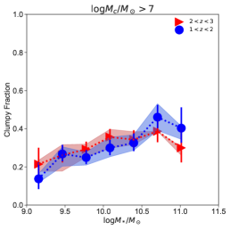
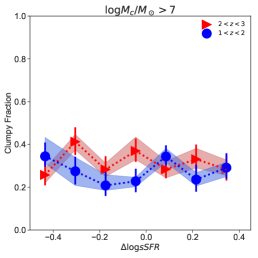
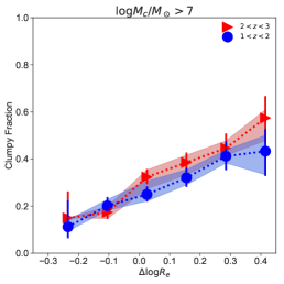
4.7.2 Simulations
We now compare the clumpy fractions, defined in both VELA and CANDELS as the fraction of galaxies hosting at least one massive clump. This is shown in figure 17. We see a general good agreement between observed and simulated datasets although simulations tend to predict clumpy fractions in the higher region of the confidence interval. Both samples indeed present clumpy fractions around in the considered redshift range. The VELA simulation presents a clear dependence of the clumpy fraction with galaxy stellar mass. More massive galaxies are almost twice as likely to host a massive clump than lower mass ones, which is also seen in CANDELS. The left panel of figure 16 in which the complete CANDELS sample is included shows this trend more clearly. Massive galaxies have larger clumpy fractions because we set a mass limit for the clumps and it is obviously less frequent to have such a massive clump when the galaxy mass is smaller. However, it seems that the VELA simulation over predicts the fraction of massive clumpy galaxies.
Interestingly, the clumpy fraction does not seem to depend on sSFR either in the simulations even if most of the clumps are formed in-situ. Regarding size dependence, we observe again that observations present a clear trend. The trend is again less pronounced in the VELA simulations.
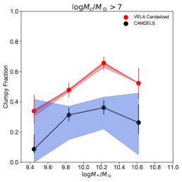
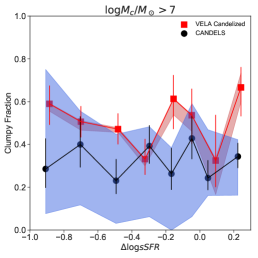
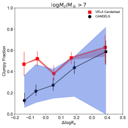
5 Summary and conclusions
In the first part of this work, we have presented a neural network based clump detector. The neural network takes a stamp of a galaxy and produces a binary image with the pixels belonging to a clump set to one. The model is trained on simple analytic simulations made of Sersic profiles with added clumps, and it reaches a purity and completeness around based on an independent test set. We have shown that the neural network model generalizes well to real data, even if trained on simulations, reaching comparable and even higher sensitivity on real observations than previously published methods and requiring less computational time.
Based on these results, we have applied the clump detector to a sample of star-forming galaxies in CANDELS in up to seven different photometric bands. The catalog of detections is released with the present work. We then derive the stellar masses of optically selected clumps through a Bayesian fit to the SEDs in two CANDELS fields (GOOD-S and GOODS-N) for which 7 photometric bands are available in the redshift range . This corresponds to galaxies and clumps. The same procedure is applied to forward modeled zoom-in cosmological simulations of 35 galaxies as they evolve in the redshift range to , including all observational effects. Properties of the clumps in the VELA simulations are
reported in Mandelker et al. (2014, 2017), which found that the vast majority of clumps form in-situ. We analyze simulated galaxies with exactly the same methods as for the observations and compare with an observational dataset of the same size and similar redshift and stellar mass distributions.
Our main results are:
-
•
Limits in angular resolution and signal to noise ratio in the photometry have a dramatic impact on the derived clumps stellar masses and therefore on the measured clump stellar mass function (cSMF) by flattening the low mass end and moving clumps towards larger masses. We have shown that this big difference between intrinsic and measured clump stellar mass functions is essentially due to a combination of incompleteness, clump blending, background light contamination, and overestimation of the clump stellar masses. This highlights the importance of comparing observations and simulations of galaxy formation under comparable conditions. It also suggests that it is difficult to extract accurate properties of individual high redshift clumps with the currently available data.
-
•
By calibrating with numerical simulations, we have shown that these effects can be partially corrected using a simple multi-layer perceptron to recover the intrinsic clump stellar mass function. We essentially perform a simple regression between the estimated SED clump mass and the 3D clump masses including some additional galaxy parameters. Once corrected, we find that the clump stellar mass function follows a power law with a slope of above the completeness limit, which we estimate at solar masses, with the majority of the clumps less massive than solar masses. Although the exact abundance of very massive clumps remains unconstrained with our data and methodology, this result tends to challenge previous observational works which found that many of the observed clumps at high redshift could be more massive than solar masses. Our clump stellar masses are also in better agreement with recent measurements based gravitational lensing.
-
•
The cSMF of simulated galaxies overall agrees with the corrected observed one when compared under the same conditions, suggesting an in-situ origin for the majority of the observed clumps. We emphasize that this agreement is independent of the corrections applied to the clump stellar masses. If simulations and observations are compared under the same conditions, without corrections, both stellar mass functions follow very similar trends.
-
•
Using corrected clump masses, we estimate that the fraction of galaxy stellar mass in massive clumps ( solar masses) is of the order of , with a slight increase at . This is smaller than the values reported for the stellar mass fractions in previous studies with incomplete datasets which did not correct for clump mass overestimation. The simulations analyzed also predict a similar fraction of mass in clumps.
-
•
We find indications that low mass galaxies ( solar masses) and larger-radius galaxies at fixed mass tend to present a larger clump contribution, which can reach up to . However, the mass fraction in clumps shows very little dependence on sSFR. The explored simulations also find a weak dependence with sSFR and an increasing contribution of clumps to the galaxy stellar mass in larger galaxies although with a weaker trend. This might be an indication of enhanced clump formation efficiency at large galacto-centric distances.
-
•
We measure that of star-forming galaxies present an off-centered clump more massive than solar masses, which also agrees reasonably well with the predictions of numerical simulations explored in this work.
The present work highlights the importance of comparing simulations and observations in a consistent way. We also have shown that with the currently available data it is very difficult to establish accurate properties of clumps, and hence the need for new observing facilities such as JWST.
In future work, we will discuss clump life times using a similar approach as the one presented here (Ginzburg et al. in prep.). We also plan to extend the comparison of clump properties to other recent simulated datasets such as the new generation of VELA simulations which uses a stronger feedback and hence has a potential impact on clumps, in order to establish statistical constraints on the feedback mechanisms. A more refined SED fitting method involving more complex star-formation histories is another potential follow-up of this work.
Acknowledgements
This material is based upon C.T. Lee’s research supported by the Chateaubriand Fellowship of the Office for Science & Technology of the Embassy of France in the United States. The research is also supported by a Google Faculty Grant awarded to Prof. Joel Primack. MHC is grateful to F. Lanusse for enlightening discussions about bayesian statistics with neural networks. NM acknowledges support from the Klauss Tschira Foundation through the HITS Yale Program in Astrophysics (HYPA). We acknowledge use of observations with the NASA/ESA Hubble Space Telescope obtained from the MAST Data Archive at the Space Telescope Science Institute, which is operated by the Association of Universities for Research in Astronomy, Incorporated, under NASA contract NAS5-26555. Support for Program number HST-AR-15798 was provided through a grant from the STScI under NASA contract NAS5-26555. The work of AD and OG was partly supported by the grants BSF 2014-273, NSF AST-1405962, GIF I-1341-303.7/2016, and DIP STE1869/2-1 GE625/17-1
Data Availability
The observational data underlying this article are part of the CANDELS survey and can be accessed here: http://arcoiris.ucolick.org/candels/. The simulations are part of the VELA simulations suite. Catalogs of metadata are available upon request. Surnise images of the VELA simulated galaxies used in this work are available online at MAST – see https://archive.stsci.edu/prepds/vela/. The derived data generated in this research, including deep learning models together with training sets and clump catalogs will be shared on reasonable request to the corresponding author.
Appendix A Effects on the clump stellar mass function of measurement errors and clump blending
One of the important results we have highlighted in this work is that the cSMFs estimated from the Candelized images differ significantly from the ones derived directly from the simulation output. In section 4, we have shown that this large difference might be due to a combination of mass measurement errors and clump blending. In this appendix, we further explore the impact of these two effects in the cSMFs using simple simulations. We start from the intrinsic 3D VELA cSMF and randomly add to the stellar mass of every clump more massive than solar masses a gaussian error of dex with a standard deviation of dex based on the results of figure 10 and recompute the cSMF with the randomly assigned masses. We repeat this 50 times. We then assume than only of the clumps are detected (figure 9) and that, on average every 2D detection corresponds to 3D clumps because of blending (fig 10) and renormalize the cSMF accordingly. The results of this exercise are shown in figure 18. The shaded region indicates the region occupied by the different realizations. We see that the Candelized cSMF and the 3D cSMF after applying the observational effects just described tend to agree much better. In particular, we see that the high mass end gets populated and that the slope is flattened. This supports our idea that the big difference between 3D and Candelized cSMFs comes from a combination of blending and mass measurement errors.
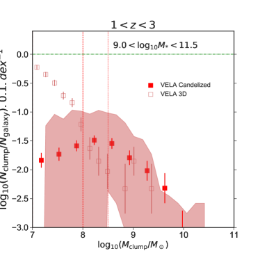
References
- Barro, et al. (2014) Barro G., et al., 2014, ApJ, 791, 52
- Barro, et al. (2019) Barro G., et al., 2019, ApJS, 243, 22
- Benincasa et al. (2019) Benincasa, S. M., Wadsley, J. W., Couchman, H. M. P., Pettitt, A. R., & Tasker, E. J. 2019, MNRAS, 486, 5022
- Bertin & Arnouts (1996) Bertin E., Arnouts S., 1996, AAS, 117, 393
- Boucaud, et al. (2020) Boucaud A., et al., 2020, MNRAS, 491, 2481
- Bournaud et al. (2007) Bournaud, F., Elmegreen, B. G., & Elmegreen, D. M. 2007, ApJ, 670, 237
- Bournaud et al. (2008) Bournaud, F., Daddi, E., Elmegreen, B. G., et al. 2008, A&A, 486, 741
- Bournaud et al. (2009) Bournaud, F., Elmegreen, B. G., & Martig, M. 2009, ApJL, 707, L1
- Bournaud et al. (2014) Bournaud, F., Perret, V., Renaud, F., et al. 2014, ApJ, 780, 57
- Bruzual & Charlot (2003) Bruzual G., Charlot S., 2003, MNRAS, 344, 1000
- Buck et al. (2016) Buck, T., Macciò, A. V., Obreja, A., et al. 2016, ArXiv e-prints
- Calzetti, et al. (2000) Calzetti D., Armus L., Bohlin R. C., Kinney A. L., Koornneef J., Storchi-Bergmann T., 2000, ApJ, 533, 682
- Cameron (2011) Cameron E., 2011, PASA, 28, 128
- Carnall, et al. (2018) Carnall A. C., McLure R. J., Dunlop J. S., Davé R., 2018, MNRAS, 480, 4379
- Cava, et al. (2018) Cava A., Schaerer D., Richard J., Pérez-González P. G., Dessauges-Zavadsky M., Mayer L., Tamburello V., 2018, NatAs, 2, 76
- Ceverino et al. (2015) Ceverino, D., Primack, J., & Dekel, A. 2015, MNRAS, 453, 408
- Ceverino et al. (2014) Ceverino, D., Klypin, A., Klimek, E. S., et al. 2014, MNRAS, 442, 1545
- Ceverino et al. (2012) Ceverino, D., Dekel, A., Mandelker, N., et al. 2012, MNRAS, 420, 3490
- Ceverino et al. (2010) Ceverino, D., Dekel, A., & Bournaud, F. 2010, MNRAS, 404, 2151
- Ceverino & Klypin (2009) Ceverino, D., & Klypin, A. 2009, ApJ, 695, 292
- Chabrier (2003) Chabrier, G. 2003, PASP, 115, 763
- Chen, et al. (2019) Chen Z., et al., 2019, arXiv, arXiv:1909.10817
- Conselice et al. (2004) Conselice, C. J., Grogin, N. A., Jogee, S., et al. 2004, ApJL, 600, L139
- Cosens et al. (2018) Cosens, M., Wright, S. A., Mieda, E., et al. 2018, ApJ, 869, 11
- Dekel, Sari & Ceverino (2009) Dekel A., Sari R., Ceverino D., 2009, ApJ, 703, 785
- Dekel & Burkert (2014) Dekel, A., & Burkert, A. 2014, MNRAS, 438, 1870
- Dekel, et al. (2020) Dekel A., et al., 2020, arXiv, arXiv:2003.08984
- Dessauges-Zavadsky et al. (2017) Dessauges-Zavadsky, M., Schaerer, D., Cava, A., Mayer, L., & Tamburello, V. 2017, ApJL, 836, L22
- Dessauges-Zavadsky & Adamo (2018) Dessauges-Zavadsky, M., & Adamo, A. 2018, MNRAS, 479, L118
- Dimauro, et al. (2018) Dimauro P., et al., 2018, MNRAS, 478, 5410
- Eddington (1913) Eddington A. S., 1913, MNRAS, 73, 359
- Elmegreen (2018) Elmegreen B. G., 2018, ApJ, 869, 119
- Elmegreen, et al. (2006) Elmegreen B. G., Elmegreen D. M., Chandar R., Whitmore B., Regan M., 2006, ApJ, 644, 879
- Elmegreen et al. (2008) Elmegreen, B. G., Bournaud, F., & Elmegreen, D. M. 2008, ApJ, 688, 67
- Elmegreen & Elmegreen (2005) Elmegreen, B. G., & Elmegreen, D. M. 2005, ApJ, 627, 632
- Elmegreen et al. (2009) Elmegreen, B. G., Elmegreen, D. M., Fernandez, M. X., & Lemonias, J. J. 2009, ApJ, 692, 12
- Elmegreen et al. (2007) Elmegreen, D. M., Elmegreen, B. G., Ravindranath, S., & Coe, D. A. 2007, ApJ, 658, 763
- Fang, et al. (2018) Fang J. J., et al., 2018, ApJ, 858, 100
- Fisher et al. (2017) Fisher, D. B., Glazebrook, K., Abraham, R. G., et al. 2017, ArXiv e-prints
- Förster Schreiber et al. (2011) Förster Schreiber, N. M., Shapley, A. E., Genzel, R., et al. 2011, ApJ, 739, 45
- Galametz, et al. (2013) Galametz A., et al., 2013, ApJS, 206, 10
- Genel et al. (2012) Genel, S., Naab, T., Genzel, R., et al. 2012, ApJ, 745, 11
- Genzel et al. (2008) Genzel, R., Burkert, A., Bouché, N., et al. 2008, ApJ, 687, 59
- Genzel et al. (2011) Genzel, R., Newman, S., Jones, T., et al. 2011, ApJ, 733, 101
- Giavalisco et al. (1996) Giavalisco, M., Steidel, C. C., & Macchetto, F. D. 1996, ApJ, 470, 189
- Grogin, et al. (2011) Grogin N. A., et al., 2011, ApJS, 197, 35
- Guo et al. (2012) Guo, Y., Giavalisco, M., Ferguson, H. C., Cassata, P., & Koekemoer, A. M. 2012, ApJ, 757, 120
- Guo, et al. (2013) Guo Y., et al., 2013, ApJS, 207, 24
- Guo et al. (2015) Guo, Y., Ferguson, H. C., Bell, E. F., et al. 2015, ApJ, 800, 39
- Guo et al. (2018) cite, Y., Rafelski, M., Bell, E. F., et al. 2018, ApJ, 853, 108
- Hausen & Robertson (2019) Hausen R., Robertson B., 2019, arXiv, arXiv:1906.11248
- Hemmati et al. (2014) Hemmati, S., Miller, S. H., Mobasher, B., et al. 2014, ApJ, 797, 108
- Hinojosa-Goñi et al. (2016) Hinojosa-Goñi, R., Muñoz-Tuñón, C., & Méndez-Abreu, J. 2016, A&A, 592, A122
- Hopkins et al. (2012) Hopkins, P. F., Kereš, D., Murray, N., Quataert, E., & Hernquist, L. 2012, MNRAS, 427, 968
- Hopkins et al. (2013) Hopkins, P. F., Kereš, D., & Murray, N. 2013, MNRAS, 432, 2639
- Hopkins et al. (2014) Hopkins, P. F., Kereš, D., Oñorbe, J., et al. 2014, MNRAS, 445, 581
- Huertas-Company, et al. (2018) Huertas-Company M., et al., 2018, ApJ, 858, 114
- Immeli et al. (2004a) Immeli, A., Samland, M., Gerhard, O., & Westera, P. 2004a, A&A, 413, 547
- Immeli et al. (2004b) Immeli, A., Samland, M., Westera, P., & Gerhard, O. 2004b, ApJ, 611, 20
- Inoue et al. (2016) Inoue, S., Dekel, A., Mandelker, N., et al. 2016, MNRAS, 456, 2052
- Ivison, et al. (2020) Ivison R. J., et al., 2020, MNRAS.tmp, doi:10.1093/mnrasl/slaa046
- Jonsson & Primack (2010) Jonsson, P., & Primack, J. R. 2010, New Astronomy, 15, 509
- Jonsson et al. (2010) Jonsson, P., Groves, B. A., & Cox, T. J. 2010, MNRAS, 403, 17
- Jonsson (2006) Jonsson, P. 2006, MNRAS, 372, 2
- Koekemoer, et al. (2011) Koekemoer A. M., et al., 2011, ApJS, 197, 36
- Kravtsov (2003) Kravtsov, A. V. 2003, ApJL, 590, L1
- Kravtsov et al. (1997) Kravtsov, A. V., Klypin, A. A., & Khokhlov, A. M. 1997, ApJS, 111, 73
- Kroupa (2001) Kroupa P., 2001, MNRAS, 322, 231
- Larson et al. (2020) Larson, K. L., Díaz-Santos, T., Armus, L., et al. 2020, ApJ, 888, 92
- Lin, et al. (2019) Lin L., et al., 2019, arXiv, arXiv:1910.10947
- Livermore et al. (2012) Livermore, R. C., Jones, T., Richard, J., et al. 2012, MNRAS, 427, 688
- Lower, et al. (2020) Lower S., Narayanan D., Leja J., Johnson B. D., Conroy C., Davé R., 2020, arXiv, arXiv:2006.03599
- Mandelker et al. (2017) Mandelker, N., Dekel, A., Ceverino, D., et al. 2017, MNRAS, 464, 635
- Mandelker et al. (2014) Mandelker, N., Dekel, A., Ceverino, D., et al. 2014, MNRAS, 443, 3675
- Meng & Gnedin (2020) Meng X., Gnedin O. Y., 2020, MNRAS, 494, 1263
- Mieda et al. (2016) Mieda, E., Wright, S. A., Larkin, J. E., et al. 2016, ApJ, 831, 78
- Moody et al. (2014) Moody, C. E., Guo, Y., Mandelker, N., et al. 2014, MNRAS, 444, 1389
- Murata et al. (2014) Murata, K. L., Kajisawa, M., Taniguchi, Y., et al. 2014, ApJ, 786, 15
- Murray et al. (2010) Murray, N., Quataert, E., & Thompson, T. A. 2010, ApJ, 709, 191
- Nayyeri, et al. (2017) Nayyeri H., et al., 2017, ApJS, 228, 7
- Noguchi (1999) Noguchi, M. 1999, ApJ, 514, 77
- Oke (1974) Oke, J. B. 1974, ApJS, 27, 21
- Oklopčić et al. (2017) Oklopčić, A., Hopkins, P. F., Feldmann, R., et al. 2017, MNRAS, 465, 952
- Pillepich, et al. (2019) Pillepich A., et al., 2019, MNRAS, 490, 3196
- Pillepich, et al. (2018) Pillepich A., et al., 2018, MNRAS, 475, 648
- Puech et al. (2009) Puech, M., Hammer, F., Flores, H., Neichel, B., & Yang, Y. 2009, A&A, 493, 899
- Puech et al. (2010) Puech, M. 2010, MNRAS, 406, 535
- Ravindranath et al. (2006) Ravindranath, S., Giavalisco, M., Ferguson, H. C., et al. 2006, ApJ, 652, 963
- Ribeiro et al. (2016) Ribeiro, B., Le Fèvre, O., Cassata, P., et al. 2016, ArXiv e-prints
- Rodríguez-Puebla, et al. (2017) Rodríguez-Puebla A., Primack J. R., Avila-Reese V., Faber S. M., 2017, MNRAS, 470, 651
- Ronneberger, Fischer & Brox (2015) Ronneberger O., Fischer P., Brox T., 2015, arXiv, arXiv:1505.04597
- Rowe, et al. (2015) Rowe B. T. P., et al., 2015, A&C, 10, 121
- Rujopakarn et al. (2019) Rujopakarn, W., Daddi, E., Rieke, G. H., et al. 2019, ApJ, 882, 107
- Santini, et al. (2015) Santini P., et al., 2015, ApJ, 801, 97
- Sersic (1968) Sersic J. L., 1968, adga.book
- Shibuya et al. (2016) Shibuya, T., Ouchi, M., Kubo, M., & Harikane, Y. 2016, ApJ, 821, 72
- Simons, et al. (2019) Simons R. C., et al., 2019, ApJ, 874, 59
- Soto et al. (2017) Soto, E., de Mello, D. F., Rafelski, M., et al. 2017, ApJ, 837, 6
- Stefanon, et al. (2017) Stefanon M., et al., 2017, ApJS, 229, 32
- Straughn et al. (2015) Straughn, A. N., Voyer, E. N., Eufrasio, R. T., et al. 2015, ApJ, 814, 97
- Tacchella, Forbes, & Caplar (2020) Tacchella S., Forbes J. C., Caplar N., 2020, MNRAS, 497, 698
- Tacchella, et al. (2016a) Tacchella, S., et al., 2016, MNRAS, 457, 2790
- Tacchella, et al. (2016b) Tacchella, S., Dekel, A., Carollo, C. M., et al. 2016b, MNRAS, 458, 242
- Tacchella et al (2015) Tacchella, S., Carollo, C. M., Renzini, A., et al. 2015, Science, 348, 314
- Tamburello et al. (2015) Tamburello, V., Mayer, L., Shen, S., & Wadsley, J. 2015, MNRAS, 453, 2490
- Tomassetti et al. (2016) Tomassetti, M., Dekel, A., Mandelker, N., et al. 2016, MNRAS, 458, 4477
- van der Wel, et al. (2012) van der Wel A., et al., 2012, ApJS, 203, 24
- van der Wel, et al. (2014) van der Wel A., et al., 2014, ApJ, 788, 28
- Whitaker, et al. (2012) Whitaker K. E., van Dokkum P. G., Brammer G., Franx M., 2012, ApJL, 754, L29
- Wuyts et al. (2012) Wuyts, S., Förster Schreiber, N. M., Genzel, R., et al. 2012, ApJ, 753, 114
- Wuyts et al. (2013) Wuyts, S., Förster Schreiber, N. M., Nelson, E. J., et al. 2013, ApJ, 779, 135
- Wuyts et al. (2014) Wuyts, E., Rigby, J. R., Gladders, M. D., & Sharon, K. 2014, ApJ, 781, 61
- Zanella, et al. (2019) Zanella A., et al., 2019, MNRAS, 489, 2792
- Zhang, et al. (2019) Zhang H., et al., 2019, MNRAS, 484, 5170
- Zick et al. (2020) Zick, T. O., Weisz, D. R., Ribeiro, B., et al. 2020, MNRAS, 493, 5653
- Zolotov et al. (2015) Zolotov, A., Dekel, A., Mandelker, N., et al. 2015, MNRAS, 450, 2327