aainstitutetext: CTP, Department of Physics and Astronomy, Seoul National University, Seoul 08826, Koreabbinstitutetext: IFIC, Universitat de València and CSIC, c./ Catedrático José Beltrán 2, E-46980 Paterna, Spainccinstitutetext: ICEPP, The University of Tokyo, Hongo, Bunkyo-ku, Tokyo, 113-0033, Japan

Higgs, top and electro-weak precision measurements at future e+esuperscript𝑒superscript𝑒e^{+}e^{-} colliders; a combined effective field theory analysis with renormalization mixing

Sunghoon Jung a    Junghwan Lee b    Martin Perelló c    Junping Tian b    Marcel Vos sunghoonj@snu.ac.kr ghe1266@snu.ac.kr martin.perello@ific.uv.es tian@icepp.s.u-tokyo.ac.jp marcel.vos@cern.ch
Abstract

This paper presents a combined analysis of the potential of a future electron-positron collider to constrain the Higgs, top and electro-weak (EW) sectors of the Standard Model Effective Field Theory (SMEFT). The leading contributions of operators involving top quarks arise mostly at one-loop suppressed order and can be captured by the renormalization group mixing with Higgs operators. We perform global fits with an extended basis of 29 parameters, including both Higgs and top operators, to the projections for the Higgs, top and electro-weak precision measurements at the International Linear Collider (ILC). The determination of the Higgs boson couplings in the 250 GeV stage of the ILC is initially severely degraded by the additional top-quark degrees of freedom, but can be nearly completely recovered by the inclusion of precise measurements of top-quark EW couplings at the LHC. The physical Higgs couplings are relatively robust, as the top mass is larger than the energy scale of EW processes. The effect of the top operators on the bounds on the Wilson coefficients is much more pronounced and may limit our ability to identify the source of deviations from the Standard Model. Robust global bounds on all Wilson coefficients are only obtained when the 500 GeV stage of the ILC is included.

1 Introduction

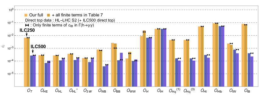
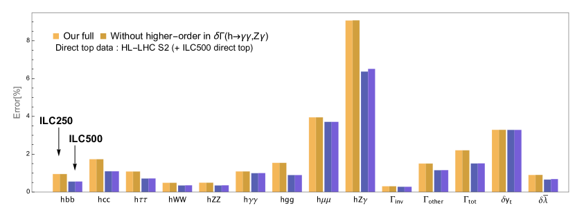
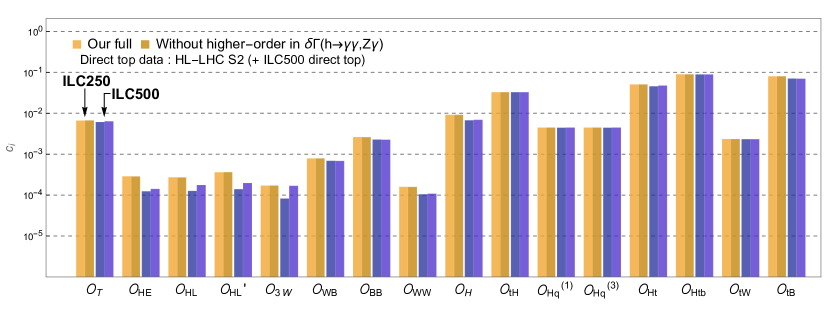
With the discovery of the Higgs boson, all particles postulated by the Standard Model (SM) of particle physics have been experimentally confirmed. Many attempts have been made to embed the SM in a more complete theory, that incorporates a description of gravity, neutrino masses, or dark matter, to name a few of the most popular targets. Currently, none of these extensions have imposed themselves as the “standard” paradigm.

In the meantime, experiments are leaving no stones unturned looking for hints of new physics. The LHC provides precise measurements of a wealth of SM processes in an unexplored energy regime. Future colliders may extend the energy reach and precision still further. We focus on an electron-positron collider with sufficient energy to produce Higgs bosons and eventually top quarks, and adopt in particular the scenario111A “Higgs factory” can also be implemented as a linear collider based on warm radio-frequency technology (CLIC Charles:2018vfv ; Linssen:2012hp ) or a 100 km ring (FCCee Abada:2019zxq , CEPC CEPCStudyGroup:2018ghi ). of the ILC Bambade:2019fyw ; Baer:2013cma .

Effective-field theory (EFT) or the Standard Model EFT (SMEFT) is a crucial tool in modern high-energy physics, as it provides a relatively model-independent framework to order and interpret the enormous wealth of measurements from experiments at colliders and elsewhere. This approach is particularly needed when one is to extract some properties in a model-independent way. Some of the earliest works along this direction have focused on LHC Higgs physics Khachatryan:2016vau ; Ellis:2018gqa ; Brivio:2016fzo and top physics Brivio:2019ius ; Hartland:2019bjb ; Durieux:2019rbz ; Buckley:2015lku ; Buckley:2015nca 222Recently, differential distributions of EW processes have also been included in SMEFT analyses Banerjee:2019twi .. EFT studies also provide a global framework to compare scenarios for future colliders in terms of the sensitivity of their precision measurements to new physics. We build on studies for future collider prospects that have been performed in the Higgs/EW Barklow:2017suo ; Barklow:2017awn and top sector Durieux:2019rbz ; Durieux:2018tev .

In this study, we combine the contributions from the Higgs/EW and top sectors that have been treated separately so far. The top-sector contributions to Higgs+EW precision observables have been ignored as they are one-loop suppressed compared to those of Higgs operators and SM. However, these are leading contributions of the top sector at the initial stages of ILC at 250 GeV , before top quarks can be directly produced.

Therefore, it is important to include top contributions and assess whether the Higgs precision achievable without model-independent top effects can be retained even with them, what capabilities of future colliders are needed, and whether the top sector can be precisely constrained without direct top productions.

To this end, we extend the previous SMEFT basis of Ref. Barklow:2017suo ; Barklow:2017awn to include seven additional operators involving top quarks. We thus include a total of 29 degrees of freedom that affect Higgs production and decay rates, EW precision measurements and high-energy di-boson production, and the EW interactions of the top quark. We include all and only leading contributions of these operators, up to log-enhanced one-loop contributions compared to the SM ones, as captured by Higgs and top operator mixing through the renormalization group (RG) evolution of Higgs operators due to top operators333The authors of Ref. Durieux:2018ggn ; Vryonidou:2018eyv have developed a similar approach and used it to study the prospects of circular electron-positron colliders. Their studies are compared with ours in Appendix B. .

We first treat the additional top operators as a threat to the Higgs fit and evaluate how the extension of the operator basis with top-quark operators affects the determination of the Higgs boson couplings. We investigate how precise measurements of top quark electro-weak couplings at the LHC or future measurements at the ILC at s=𝑠absent\sqrt{s}= 500 GeV can mitigate this effect. We also consider the new opportunity that the interplay between top and Higgs physics offers. We discuss to what extent the 250 GeV “Higgs factory” programme can do top physics without actually producing top quarks by using Higgs/EW precision measurements to set indirect bounds on the top operator coefficients.

The paper is structured as follows. In Section 2 and Section 3 we present the motivation and the theory framework, with details of the operator basis, power counting of top effects, and renormalization group effects. Section 4 presents the benchmark datasets that are used in the fit. The main results are presented in Section 5. In Section 6, we summarize the most important findings of the study and discuss their implications.

2 Motivation and background

The top-sector’s contributions to the Higgs+EW observables are the leading top contributions to the initial “Higgs factory” stage of future electron-positron colliders. There are various good reasons to expect that top-sector contributions can be important, numerically.

2.1 Top-Higgs interplay in the SM

In practice, we expect the most important next-to-lowest effects would come from loop effects induced by top-quark related operators. It is first because the top-EW interactions are only poorly constrained by the LHC and the initial (250 GeV) stage of future Higgs factories does not reach the top quark pair production threshold.

e+superscript𝑒e^{+}esuperscript𝑒e^{-}Z𝑍Zhht𝑡t
Z𝑍Ze+superscript𝑒e^{+}esuperscript𝑒e^{-}t𝑡t
γ𝛾\gammahhγ𝛾\gammat𝑡t
Figure 1: Example loop diagrams involving top quarks in e+eZhsuperscript𝑒superscript𝑒𝑍e^{+}e^{-}\to Zh production (left), Ze+e𝑍superscript𝑒superscript𝑒Z\to e^{+}e^{-} (middle) and hγγ𝛾𝛾h\to\gamma\gamma (right). The solid black dots indicate vertices that are affected by the operators considered in this paper.

Figure 1 shows three example loop processes where top-EW couplings can contribute. The contribution of top-loop diagrams involving poorly constrained operators can easily exceed the experimental accuracies of the rate measurements for those processes. The first diagram contributes directly to the dominant Higgs production process, and would hence affect the Higgs coupling measurements. The second diagram contributes to the Z𝑍Z-pole process and will play a role in electro-weak precision observables444For an analogy, consider the W𝑊W-mass measurement. The SM computation of mWsubscript𝑚𝑊m_{W} receives an uncertainty from top mass uncertainty (ΔmWsimilar-toΔsubscript𝑚𝑊absent\Delta m_{W}\sim 6 MeV for Δmtsimilar-toΔsubscript𝑚𝑡absent\Delta m_{t}\sim 1 GeV  Awramik:2003rn ). At a certain precision of mWsubscript𝑚𝑊m_{W}, further improvements of the experimental measurement will not increase the precision of the comparison, unless one can improve the top-quark mass measurement as well. (EWPO). The third diagram contributes to the hγγ𝛾𝛾h\to\gamma\gamma branching ratio.

hhγ𝛾\gammaγ𝛾\gammat𝑡t
hhg𝑔gg𝑔gt𝑡t
hhγ𝛾\gammaZ𝑍Zt𝑡t
Figure 2: Loop diagrams for Higgs boson interactions with photons (left), gluons (middle), and with a photon and Z𝑍Z-boson (right). The solid black dots indicate vertices that are affected by the operators considered in this paper.

Another reason is that the top quark couples to the SM most strongly. This makes the top-loop the dominant contribution to the loop-induced Higgs decays and productions in the SM, as shown in Fig. 2. In a calculation that explicitly resolves the loop diagrams, the three diagrams depend on various top-EW couplings, including the tt¯h𝑡¯𝑡t\bar{t}h, tt¯γ𝑡¯𝑡𝛾t\bar{t}\gamma, tt¯g𝑡¯𝑡𝑔t\bar{t}g, and tt¯Z𝑡¯𝑡𝑍t\bar{t}Z vertices555Indeed, in the so-called resolved version of the fit in κ𝜅\kappa framework used for early LHC analyses Khachatryan:2016vau the scale factors for the effective Higgs boson coupling to gluons are written as κgκt+Δκgsimilar-tosubscript𝜅𝑔subscript𝜅𝑡Δsubscript𝜅𝑔\kappa_{g}\sim\kappa_{t}+\Delta\kappa_{g} and that to photons as κγ0.28κt+1.28κW+Δκγsimilar-tosubscript𝜅𝛾0.28subscript𝜅𝑡1.28subscript𝜅𝑊Δsubscript𝜅𝛾\kappa_{\gamma}\sim-0.28\kappa_{t}+1.28\kappa_{W}+\Delta\kappa_{\gamma} Dawson:2013bba , where κtsubscript𝜅𝑡\kappa_{t} and κWsubscript𝜅𝑊\kappa_{W} are the scale factors that multiply the SM predictions for the Higgs boson couplings to the top quark and the W𝑊W-boson (κg=κγ=κt=κW=1subscript𝜅𝑔subscript𝜅𝛾subscript𝜅𝑡subscript𝜅𝑊1\kappa_{g}=\kappa_{\gamma}=\kappa_{t}=\kappa_{W}=1 and Δκg=Δκγ=0Δsubscript𝜅𝑔Δsubscript𝜅𝛾0\Delta\kappa_{g}=\Delta\kappa_{\gamma}=0 in the SM).. Also, such vertex contributions are not loop suppressed compared to those of SM ones. Therefore, Higgs precision measurements can be sensitive to new physics that affect the top-EW vertices. Higgs factories operating at s=𝑠absent\sqrt{s}= 250 GeV can probe these vertices indirectly. The inclusion of these loop effects is described in Section 3.6 and a quantitative analysis is presented in Section 5.8 and Section 5.7.

2.2 BSM motivation

A further entanglement of the Higgs and top sectors may arise in new physics models beyond the SM (BSM). Generally speaking, extensions of the Standard Model are under no obligation to respect the separation between the top and Higgs sectors. Rather, concrete extensions of the SM do activate multiple operators across several sectors.

A well-known example is found in composite Higgs models Agashe:2004rs ; Kaplan:1983fs . The Higgs boson couplings are expected to deviate from the SM predictions as κ1c×1TeVfsimilar-to𝜅1𝑐1TeV𝑓\kappa\sim 1-c\times\frac{1\,{\mathrm{Te\kern-0.70004ptV}}\,}{f}, where f𝑓f is the scale associated with the new physics and csimilar-to𝑐absentc\sim 3% for vector boson couplings and csimilar-to𝑐absentc\sim 3 – 9% for fermion couplings Dawson:2013bba . As the top quark is the heaviest SM particle and consequently tends to mix strongly with the composite sector, the top-EW couplings are typically altered sizably. A custodial symmetry is usually invoked to protect the coupling of the Z𝑍Z-boson to left-handed bottom quarks, but cannot simultaneously avoid large corrections to the EW couplings of the top quark Agashe:2006at ; Grojean:2013qca . Ref. Richard:2014upa indeed collects a number of concrete proposals for composite Higgs models that predict sizeable (up to 10-20%) deviations from the SM for the top quark couplings to the Z𝑍Z-boson. Ref. Durieux:2018ekg quantitatively demonstrated that the measurements of Higgs boson and top (and bottom) quark couplings provide complementary handles. Together, precise measurements of the top, Higgs and EW sectors probe the parameter space of typical models up to a scale well beyond the direct reach of colliders. A comprehensive study of the constraints of precision measurements on such models requires a combined analyses of Higgs and top measurements.

3 Theoretical framework

In this section, we present the extended basis of dimension-six operators, including the Higgs operators proposed in Ref. Barklow:2017awn and additional top operators. Then we detail various top-quark effects that we include, with the power counting rules to select which top effects to include with the renormalization group calculation.

3.1 Higgs/EW operators

Following Barklow:2017awn , we use the 10 ‘Higgs’ operators below to parameterize the lowest-order modifications of Higgs and EW observables.

𝒪H=μ(ΦΦ)μ(ΦΦ),subscript𝒪𝐻superscript𝜇superscriptΦΦsubscript𝜇superscriptΦΦ\displaystyle\mathcal{O}_{H}=\partial^{\mu}(\Phi^{\dagger}\Phi)\partial_{\mu}(\Phi^{\dagger}\Phi),~{}~{}~{} 𝒪T=(ΦDμΦ)(ΦDμΦ),subscript𝒪𝑇superscriptΦsuperscript𝐷𝜇ΦsuperscriptΦsubscript𝐷𝜇Φ\displaystyle~{}~{}~{}\mathcal{O}_{T}=(\Phi^{\dagger}\overleftrightarrow{D}^{\mu}\Phi)(\Phi^{\dagger}\overleftrightarrow{D}_{\mu}\Phi), (1)
𝒪6=(ΦΦ)3,subscript𝒪6superscriptsuperscriptΦΦ3\displaystyle\mathcal{O}_{6}=(\Phi^{\dagger}\Phi)^{3},~{}~{}~{} 𝒪WB=ΦtaΦWμνaBμν,subscript𝒪𝑊𝐵superscriptΦsuperscript𝑡𝑎Φsuperscriptsubscript𝑊𝜇𝜈𝑎superscript𝐵𝜇𝜈\displaystyle~{}~{}~{}\mathcal{O}_{WB}=\Phi^{\dagger}t^{a}\Phi W_{\mu\nu}^{a}B^{\mu\nu},
𝒪BB=ΦΦBμνBμν,subscript𝒪𝐵𝐵superscriptΦΦsubscript𝐵𝜇𝜈superscript𝐵𝜇𝜈\displaystyle\mathcal{O}_{BB}=\Phi^{\dagger}\Phi B_{\mu\nu}B^{\mu\nu},~{}~{}~{} 𝒪3W=ϵabcWμνaWρbνWcρμ,subscript𝒪3𝑊subscriptitalic-ϵ𝑎𝑏𝑐superscriptsubscript𝑊𝜇𝜈𝑎superscriptsubscript𝑊𝜌𝑏𝜈superscript𝑊𝑐𝜌𝜇\displaystyle~{}~{}~{}\mathcal{O}_{3W}=\epsilon_{abc}W_{\mu\nu}^{a}W_{\rho}^{b\nu}W^{c\rho\mu},
𝒪HL=(ΦiDμΦ)(L¯γμL),subscript𝒪𝐻𝐿superscriptΦ𝑖superscript𝐷𝜇Φ¯𝐿subscript𝛾𝜇𝐿\displaystyle\mathcal{O}_{HL}=(\Phi^{\dagger}i\overleftrightarrow{D}^{\mu}\Phi)(\bar{L}\gamma_{\mu}L),~{}~{}~{} 𝒪HL=(ΦtaiDμΦ)(L¯γμtaL),subscript𝒪𝐻superscript𝐿superscriptΦsuperscript𝑡𝑎𝑖superscript𝐷𝜇Φ¯𝐿subscript𝛾𝜇superscript𝑡𝑎𝐿\displaystyle~{}~{}~{}\mathcal{O}_{HL^{\prime}}=(\Phi^{\dagger}t^{a}i\overleftrightarrow{D}^{\mu}\Phi)(\bar{L}\gamma_{\mu}t^{a}L),
𝒪HE=(ΦiDμΦ)(e¯γμe),subscript𝒪𝐻𝐸superscriptΦ𝑖superscript𝐷𝜇Φ¯𝑒subscript𝛾𝜇𝑒\displaystyle\mathcal{O}_{HE}=(\Phi^{\dagger}i\overleftrightarrow{D}^{\mu}\Phi)(\bar{e}\gamma_{\mu}e),~{}~{}~{} 𝒪WW=(ΦΦ)WμνaWaμν,subscript𝒪𝑊𝑊superscriptΦΦsuperscriptsubscript𝑊𝜇𝜈𝑎superscript𝑊𝑎𝜇𝜈\displaystyle~{}~{}~{}\mathcal{O}_{WW}=(\Phi^{\dagger}\Phi)W_{\mu\nu}^{a}W^{a\mu\nu},

with the Lagrangian terms

ΔHiggs=ΔsubscriptHiggsabsent\displaystyle\Delta\mathcal{L}_{\rm Higgs}\,=\, cH2v2𝒪H+cT2v2𝒪Tc6λv2𝒪6+g2cWWmW2𝒪WW+4ggcWBmW2𝒪WB+g2cBBmW2𝒪BBsubscript𝑐𝐻2superscript𝑣2subscript𝒪𝐻subscript𝑐𝑇2superscript𝑣2subscript𝒪𝑇subscript𝑐6𝜆superscript𝑣2subscript𝒪6superscript𝑔2subscript𝑐𝑊𝑊superscriptsubscript𝑚𝑊2subscript𝒪𝑊𝑊4𝑔superscript𝑔subscript𝑐𝑊𝐵superscriptsubscript𝑚𝑊2subscript𝒪𝑊𝐵superscript𝑔2subscript𝑐𝐵𝐵superscriptsubscript𝑚𝑊2subscript𝒪𝐵𝐵\displaystyle\frac{c_{H}}{2v^{2}}\mathcal{O}_{H}\,+\,\frac{c_{T}}{2v^{2}}\mathcal{O}_{T}\,-\,\frac{c_{6}\lambda}{v^{2}}\mathcal{O}_{6}\,+\,\frac{g^{2}c_{WW}}{m_{W}^{2}}\mathcal{O}_{WW}\,+\,\frac{4gg^{\prime}c_{WB}}{m_{W}^{2}}\mathcal{O}_{WB}\,+\,\frac{g^{\prime 2}c_{BB}}{m_{W}^{2}}\mathcal{O}_{BB} (2)
+g3c3WmW2𝒪3W+cHLv2𝒪HL+4cHLv2𝒪HL+cHEv2𝒪HE,superscript𝑔3subscript𝑐3𝑊superscriptsubscript𝑚𝑊2subscript𝒪3𝑊subscript𝑐𝐻𝐿superscript𝑣2subscript𝒪𝐻𝐿4superscriptsubscript𝑐𝐻𝐿superscript𝑣2subscript𝒪𝐻superscript𝐿subscript𝑐𝐻𝐸superscript𝑣2subscript𝒪𝐻𝐸\displaystyle\,+\,\frac{g^{3}c_{3W}}{m_{W}^{2}}\mathcal{O}_{3W}\,+\,\frac{c_{HL}}{v^{2}}\mathcal{O}_{HL}\,+\,\frac{4c_{HL}^{\prime}}{v^{2}}\mathcal{O}_{HL^{\prime}}\,+\,\frac{c_{HE}}{v^{2}}\mathcal{O}_{HE},

where the Higgs vacuum expectation value v=246𝑣246v=246 GeV and ta=12τasuperscript𝑡𝑎12superscript𝜏𝑎t^{a}=\frac{1}{2}\tau^{a} (τasuperscript𝜏𝑎\tau^{a} are Pauli matrices). We do not assume oblique Peskin:1990zt ; Peskin:1991sw or universal Wells:2015uba corrections and treat all ten operators as independent. We also add Yukawa operators cbH,cH,τH,μH,subscript𝑐𝑏𝐻𝑐𝐻𝜏𝐻𝜇𝐻c_{bH,\,cH,\,\tau H,\,\mu H,} to the SM fermions (e.g. 𝒪bH=(ΦΦ)(Q¯bΦ)subscript𝒪𝑏𝐻superscriptΦΦ¯𝑄𝑏Φ\mathcal{O}_{bH}=(\Phi^{\dagger}\Phi)(\bar{Q}b\Phi)) and the collective gluonic operators cgHsubscript𝑐𝑔𝐻c_{gH} and 𝒞W,Zsubscript𝒞𝑊𝑍{\cal C}_{W,\,Z} to effectively describe the Higgs decay widths and corresponding physical Higgs couplings. We refer to Ref. Barklow:2017awn for a detailed discussion of this operator set.

We denote δA=ΔA/A𝛿𝐴Δ𝐴𝐴\delta A=\Delta A/A as the deviation of the observable A𝐴A from its SM prediction. We express δA𝛿𝐴\delta A in terms of EFT coefficients. We also define the deviation of the physical Higgs coupling as the deviation of the square-root of the partial width Barklow:2017awn ; deBlas:2019wgy

δg(hXX)12δΓ(hXX),𝛿𝑔𝑋𝑋12𝛿Γ𝑋𝑋\delta g(hXX)\,\equiv\,\frac{1}{2}\delta\Gamma(h\to XX), (3)

where X𝑋X can be any particles to which the Higgs boson decays. For example,

δg(hbb¯)=12δΓ(hbb¯)=12(2cbH 2δv+δZh+δmh),𝛿𝑔𝑏¯𝑏12𝛿Γ𝑏¯𝑏122subscript𝑐𝑏𝐻2𝛿𝑣𝛿subscript𝑍𝛿subscript𝑚\delta g(hb\bar{b})\,=\,\frac{1}{2}\delta\Gamma(h\to b\bar{b})\,=\,\frac{1}{2}(2c_{bH}\,-\,2\delta v\,+\,\delta Z_{h}\,+\,\delta m_{h}), (4)

where we explicitly write the dependence on δmh𝛿subscript𝑚\delta m_{h} and δv𝛿𝑣\delta v, and δZh=cH𝛿subscript𝑍subscript𝑐𝐻\delta Z_{h}=-c_{H} is the correction to the Higgs field strength. This expression is slightly different from that of Ref. Barklow:2017awn where cbHsubscript𝑐𝑏𝐻c_{bH} was used to collectively describe cbH,δvsubscript𝑐𝑏𝐻𝛿𝑣c_{bH},\,\delta v and δmh𝛿subscript𝑚\delta m_{h} altogether. They are separated to emphasize the dependence on the three parameters, but numerical results remain almost unchanged. We use a similar treatment for δg(hμ+μ),δg(hτ+τ),δg(hcc¯)𝛿𝑔superscript𝜇superscript𝜇𝛿𝑔superscript𝜏superscript𝜏𝛿𝑔𝑐¯𝑐\delta g(h\mu^{+}\mu^{-}),\,\delta g(h\tau^{+}\tau^{-}),\,\delta g(hc\bar{c}).

The Higgs self-coupling is represented by λ¯¯𝜆\overline{\lambda} defined as

λ¯=λ(1+32c6),¯𝜆𝜆132subscript𝑐6\overline{\lambda}\,=\,\lambda\,\left(1\,+\,\frac{3}{2}c_{6}\right), (5)

which is a combination of the original Higgs self-coupling λ𝜆\lambda and the operator c6subscript𝑐6c_{6} shifting the Higgs potential. In the Higgs fit at s=𝑠absent\sqrt{s}= 250 GeV , λ¯¯𝜆\overline{\lambda} is constrained by the Higgs mass measurement. Only this combination appears in our global fit until the di-Higgs production e+eZhhsuperscript𝑒superscript𝑒𝑍e^{+}e^{-}\rightarrow Zhh is available at s=𝑠absent\sqrt{s}= 500 GeV . Although the Higgs pair production at HL-LHC can provide some handle, the ILC σ(Zhh)𝜎𝑍\sigma(Zhh) measurement will eventually provide the most precise and robust determination of c6subscript𝑐6c_{6} independently from λ𝜆\lambda DiVita:2017vrr . Instead, for the early stage of the ILC at s=𝑠absent\sqrt{s}= 250 GeV , it is assumed that the HL-LHC data constrain c6subscript𝑐6c_{6} well enough, so as not to affect the model-independent fit of other parameters Durieux:2018ggn . It was also proposed to use the finite one-loop corrections of c6subscript𝑐6c_{6} to the Higgsstrahlung process e+eZhsuperscript𝑒superscript𝑒𝑍e^{+}e^{-}\to Zh at ILC250 McCullough:2013rea ; DiVita:2017eyz to constrain c6subscript𝑐6c_{6}. This contribution is not considered in the power counting we adopt (more on this in Section 3.4). A more dedicated study could be interesting.

3.2 Top operators

To properly account for the dependence of Higgs precision observables on vertices involving top quarks, we include the following seven ‘top’ operators in our basis.

𝒪tH=(ΦΦ)(Q¯tΦ~),subscript𝒪𝑡𝐻superscriptΦΦ¯𝑄𝑡~Φ\displaystyle\mathcal{O}_{tH}=(\Phi^{\dagger}\Phi)(\bar{Q}t\tilde{\Phi}),~{}~{}~{} 𝒪Hq(1)=(ΦiDμΦ)(Q¯γμQ),superscriptsubscript𝒪𝐻𝑞1superscriptΦ𝑖subscript𝐷𝜇Φ¯𝑄superscript𝛾𝜇𝑄\displaystyle~{}~{}~{}\mathcal{O}_{Hq}^{(1)}=(\Phi^{\dagger}i\overleftrightarrow{D}_{\mu}\Phi)(\bar{Q}\gamma^{\mu}Q), (6)
𝒪Hq(3)=(ΦiDμaΦ)(Q¯γμτaQ),superscriptsubscript𝒪𝐻𝑞3superscriptΦ𝑖superscriptsubscript𝐷𝜇𝑎Φ¯𝑄superscript𝛾𝜇superscript𝜏𝑎𝑄\displaystyle\mathcal{O}_{Hq}^{(3)}=(\Phi^{\dagger}i\overleftrightarrow{D}_{\mu}^{a}\Phi)(\bar{Q}\gamma^{\mu}\tau^{a}Q),~{}~{}~{} 𝒪Ht=(ΦiDμΦ)(t¯γμt),subscript𝒪𝐻𝑡superscriptΦ𝑖subscript𝐷𝜇Φ¯𝑡superscript𝛾𝜇𝑡\displaystyle~{}~{}~{}\mathcal{O}_{Ht}=(\Phi^{\dagger}i\overleftrightarrow{D}_{\mu}\Phi)(\bar{t}\gamma^{\mu}t),
𝒪Htb=(Φ~iDμΦ)(t¯γμb),subscript𝒪𝐻𝑡𝑏superscript~Φ𝑖subscript𝐷𝜇Φ¯𝑡superscript𝛾𝜇𝑏\displaystyle\mathcal{O}_{Htb}=(\tilde{\Phi}^{\dagger}iD_{\mu}\Phi)(\bar{t}\gamma^{\mu}b),
𝒪tW=(Q¯σμνt)τaΦ~Wμνa,subscript𝒪𝑡𝑊¯𝑄superscript𝜎𝜇𝜈𝑡superscript𝜏𝑎~Φsuperscriptsubscript𝑊𝜇𝜈𝑎\displaystyle\mathcal{O}_{tW}=(\bar{Q}\sigma^{\mu\nu}t)\tau^{a}\tilde{\Phi}W_{\mu\nu}^{a},~{}~{}~{} 𝒪tB=(Q¯σμνt)Φ~Bμν,subscript𝒪𝑡𝐵¯𝑄superscript𝜎𝜇𝜈𝑡~Φsubscript𝐵𝜇𝜈\displaystyle~{}~{}~{}\mathcal{O}_{tB}=(\bar{Q}\sigma^{\mu\nu}t)\tilde{\Phi}B_{\mu\nu},

with

Δtop=ytctHv2𝒪tH+cHq(1)v2𝒪Hq(1)+cHq(3)v2𝒪Hq(3)+cHtv2𝒪Ht+cHtbv2𝒪Htb+ctWv2𝒪tW+ctBv2𝒪tB,Δsubscripttopsubscript𝑦𝑡subscript𝑐𝑡𝐻superscript𝑣2subscript𝒪𝑡𝐻superscriptsubscript𝑐𝐻𝑞1superscript𝑣2superscriptsubscript𝒪𝐻𝑞1superscriptsubscript𝑐𝐻𝑞3superscript𝑣2superscriptsubscript𝒪𝐻𝑞3subscript𝑐𝐻𝑡superscript𝑣2subscript𝒪𝐻𝑡subscript𝑐𝐻𝑡𝑏superscript𝑣2subscript𝒪𝐻𝑡𝑏subscript𝑐𝑡𝑊superscript𝑣2subscript𝒪𝑡𝑊subscript𝑐𝑡𝐵superscript𝑣2subscript𝒪𝑡𝐵\Delta\mathcal{L}_{\rm top}=-y_{t}\frac{c_{tH}}{v^{2}}\mathcal{O}_{tH}+\frac{c_{Hq}^{(1)}}{v^{2}}\mathcal{O}_{Hq}^{(1)}+\frac{c_{Hq}^{(3)}}{v^{2}}\mathcal{O}_{Hq}^{(3)}+\frac{c_{Ht}}{v^{2}}\mathcal{O}_{Ht}+\frac{c_{Htb}}{v^{2}}\mathcal{O}_{Htb}+\frac{c_{tW}}{v^{2}}\mathcal{O}_{tW}+\frac{c_{tB}}{v^{2}}\mathcal{O}_{tB}, (7)

where Q𝑄Q is the third-generation left-handed quark doublet and Φ~=iτ2Φ~Φ𝑖subscript𝜏2superscriptΦ\tilde{\Phi}=i\tau_{2}\Phi^{\dagger}. These are the top operators that affect Higgs and EW observables at one loop. We do not consider four-fermion operators that involve two top quarks. In this work, we calculate these one-loop effects using the Renormalization Group (RG) evolution and mixing of top and Higgs operators. Our power counting rule is discussed in Section 3.4, top RG effects in Section 3.5, and top effects that are not captured in this way in Section 3.6.

In several extensions of the Standard Model, the effect of the top operators may be accompanied by bottom-quark effects. We have evaluated the one-loop effects on the global fit and find them to be negligible. This is discussed in detail in Appendix E.

3.3 Top Yukawa coupling

The operator coefficient ctHsubscript𝑐𝑡𝐻c_{tH} shifts the top Yukawa coupling and the top mass at tree level. Including also Higgs operator contributions, we can write the following expression:

ΔΔ\displaystyle\Delta{\cal L} =\displaystyle= ytv2(1+12ctH)t¯tyt2(1+32ctH+12δZh)ht¯tsubscript𝑦𝑡𝑣2112subscript𝑐𝑡𝐻¯𝑡𝑡subscript𝑦𝑡2132subscript𝑐𝑡𝐻12𝛿subscript𝑍¯𝑡𝑡\displaystyle-\frac{y_{t}v}{\sqrt{2}}(1+\tfrac{1}{2}c_{tH})\bar{t}t\,-\,\frac{y_{t}}{\sqrt{2}}(1+\tfrac{3}{2}c_{tH}+\tfrac{1}{2}\delta Z_{h})h\bar{t}t (8)
=\displaystyle= mtt¯tmtv(1+ctH12cH)ht¯t.subscript𝑚𝑡¯𝑡𝑡subscript𝑚𝑡𝑣1subscript𝑐𝑡𝐻12subscript𝑐𝐻¯𝑡𝑡\displaystyle-m_{t}\bar{t}t\,-\,\frac{m_{t}}{v}(1+c_{tH}-\frac{1}{2}c_{H})h\bar{t}t. (9)

In the second line, we define the top mass as mt=ytv/2(1+12ctH)subscript𝑚𝑡subscript𝑦𝑡𝑣2112subscript𝑐𝑡𝐻m_{t}=y_{t}v/\sqrt{2}(1+\tfrac{1}{2}c_{tH}) and rewrite the Yukawa coupling in terms of the redefined top mass. Thus, we define the deviation of the top-quark Yukawa coupling as

δytctH12cHδv.𝛿subscript𝑦𝑡subscript𝑐𝑡𝐻12subscript𝑐𝐻𝛿𝑣\delta y_{t}\,\equiv\,c_{tH}\,-\,\frac{1}{2}c_{H}\,-\,\delta v. (10)

The top-quark Yukawa coupling and its tree-level modification can be measured separately from the top mass and the tt¯h𝑡¯𝑡t\bar{t}h cross-section. The latter is available at the LHC and HL-LHC prospects will be used throughout in this work. The ILC can measure the top-quark Yukawa coupling directly at s=500𝑠500\sqrt{s}=500 GeV stage (or, even better, 550 GeV Fujii:2019zll ). The top-quark Yukawa coupling also affects Higgs decays hγγ,Zγ,gg𝛾𝛾𝑍𝛾𝑔𝑔h\to\gamma\gamma,\,Z\gamma,\,gg via one-loop diagrams, which are available already at the low-energy running of ILC Boselli:2018zxr . These are finite one-loop effects, but are important because SM contributions are also at one-loop. They are indeed included in our work consistently with the power-counting rule in Section 3.4 and further discussed in Section 3.6.

The coefficient ctHsubscript𝑐𝑡𝐻c_{tH} appears in our global fits only through the top Yukawa coupling as in Eq. (10). It does not RG mix with any Higgs operators. The only exception is c6subscript𝑐6c_{6} (as shown in Eq. (56)), but ctHsubscript𝑐𝑡𝐻c_{tH}’s RG contributions cannot be measured in our global fits since c6subscript𝑐6c_{6} appears only at one energy scale (i.e. from the Zhh𝑍Zhh production cross section at s=𝑠absent\sqrt{s}= 500 GeV ). Thus, we do not include the RG evolution of c6subscript𝑐6c_{6}.

3.4 Power counting for top-loop contributions

In this work, we consider a subset of the leading effects of top operators on precision measurements of Higgs and EW sectors. Although it is best to include the full leading effects, most of them are loop contributions, and hence not easy to calculate and understand. As a first step toward a complete study, it is better to focus on a consistent subset of important effects. This subsection develops a power counting to select such a subset.

One could hope to include all top contributions at a given absolute order. The one-loop corrections then unambiguously specify the top contributions from one-loop diagrams. But the fact that not all leading SM processes are generated at the same absolute order makes the issue complicated. Consider the Higgs decays hγγ,Zγ,gg𝛾𝛾𝑍𝛾𝑔𝑔h\to\gamma\gamma,Z\gamma,gg versus the other Higgs processes. In the SM, the former are generated at one-loop while the latter are already present at tree-level. In a numerical analysis, we do include all those processes and treat them equally even though their absolute orders are different. It is because they are leading contributions to each observable. The underlying logic is that if measurement uncertainties of tree- and loop-induced observables are similar, those leading contributions will receive similar constraints, regardless of their absolute orders. Thus, they will be similarly important. The leading contribution has an important role, irrespective of its absolute order; it provides a new information for the first time, while subleading corrections usually only modify the leading information.

The same issue applies to top contributions to Higgs physics observables. Although we will be interested in leading top contributions regardless of their absolute orders, not all leading contributions are equally important. If the leading top contribution arises at five-loop level, while the SM process is at tree-level, it is very unlikely that such leading top contribution have an impact, unless the observable is measured with exquisite precision. Here comes the notion of the relative orders of top contributions compared to the SM.

In all, our rule is to include all and only leading top contributions up to the logarithmic one-loop order relative to the SM. Most leading top effects arise at the one-loop order compared to the SM. Among the full one-loop corrections to SM processes, our rule is to include only logarithmic ones, which can be readily obtained through the RG evolution of Higgs operators induced by top operators. In other words, we include leading top effects up to the logarithmic one-loop compared to the SM. Whenever some Higgs operator contributes to some Higgs observables, its RG mixing with top operators accounts for those top operators’ logarithmic one-loop corrections to the observables. This is our main method to include the leading top-loop effects in this work.

The logarithmic corrections are not full one-loop effects, but they are a convenient and self-consistent subset. The RG effects respect all the symmetries of the theory, including gauge invariance, so that most non-zero effects in the full one-loop corrections also arise in RG666Some external momentum dependences of full one-loop effects are not captured by RG calculations. Such dependences can induce useful information on differential and energy-dependent observables.. Due to the logarithm of scale ratios (e.g. Eq. (12)), the RG contributions are often the dominant contribution among full one-loop effects, although this is not always the case.

This approach is convenient because the RG evolution is much easier to calculate. It needs to be calculated only once for all operators, independently of the observables, while every new full one-loop effects must be calculated separately (the majority has been done Zhang:2012cd ; Vryonidou:2018eyv ; Durieux:2018ggn ). Moreover, their contribution is easier to understand, e.g. based on operator mixing patterns Grojean:2013kd ; Jung:2014kxa . Thus, although full one-loop analysis will have to be eventually done (see, e.g. Durieux:2018ggn ), at this early stage we use RG effects as a convenient proxy for the leading top effects.

The power counting rule we propose is particularly useful if all observables are measured with similar errors. All leading contributions will receive similar constraints, regardless of their absolute orders. But if some observables are measured better, this logic may become biased. There is no obvious mathematical answer for which top contributions at which order must be included. At least, the RG parts are theoretically consistent and practically convenient proxies of leading loop effects.

There is a notable exception and subtlety with this power counting rule. It arises again from the fact that not all top contributions are at the same absolute and relative orders. Although SM hγγ,Zγ𝛾𝛾𝑍𝛾h\to\gamma\gamma,Z\gamma are induced at one-loop, cWW,WB,BBsubscript𝑐𝑊𝑊𝑊𝐵𝐵𝐵c_{WW,WB,BB} contribute at the (absolute) tree-level. Then, according to the power counting rule, two-loop RG evolutions of cWW,WB,BBsubscript𝑐𝑊𝑊𝑊𝐵𝐵𝐵c_{WW,WB,BB} and finite one-loop corrections are needed. But we include only one-loop RG evolutions of cWW,WB,BBsubscript𝑐𝑊𝑊𝑊𝐵𝐵𝐵c_{WW,WB,BB}. This may leave some numerical uncertainties.

Some top effects are not captured by the renormalization of Higgs operators. As discussed in Section 3.3 and Section 3.6, there are tree-level shifts of SM parameters due to top operators: ctHsubscript𝑐𝑡𝐻c_{tH} shifts the top Yukawa, and cHq(1),cHq(3),cHtsuperscriptsubscript𝑐𝐻𝑞1superscriptsubscript𝑐𝐻𝑞3subscript𝑐𝐻𝑡c_{Hq}^{(1)},c_{Hq}^{(3)},c_{Ht} shift the Ztt¯𝑍𝑡¯𝑡Zt\bar{t} coupling at the tree-level. We include such relative tree-level effects.

The power counting and the corrections that we include are summarized in Table 1. We also assess the numerical impact of our power counting rules in Appendices. First, the top contributions treated differently in our approach and in Durieux:2018ggn ; Vryonidou:2018eyv are compared in Appendix B; second, the uncertainties in our global fit introduced by the choice of RG scale Q𝑄Q (see next subsection) are estimated in Appendix C. We can conclude that the differences between different approaches are mostly within 𝒪(10)𝒪10{\cal O}(10)% and our results are stable with respect to the variation of Q𝑄Q.

Higgs loop production/decay other observables top production
SM finite 1-loop tree-level tree-level
Higgs operator tree-level from cWW,WB,BBsubscript𝑐𝑊𝑊𝑊𝐵𝐵𝐵c_{WW,WB,BB} tree-level none
finite 1-loop from other operators
top operator log 1-loop via c˙WW,WB,BBsubscript˙𝑐𝑊𝑊𝑊𝐵𝐵𝐵\dot{c}_{WW,WB,BB} log 1-loop via c˙˙𝑐\dot{c} tree-level
log 2-loop via other c˙˙𝑐\dot{c}
finite 1-loop via tree-shift of yt,gZttsubscript𝑦𝑡subscript𝑔𝑍𝑡𝑡y_{t},g_{Ztt}
Table 1: Summary of the absolute orders of the contributions that we include. Our power counting is discussed in Section 3.4; the RG-induced logarithmic loop effects of top operators in Section 3.5; the finite one-loop effects of top operators in loop-induced Higgs decays in Section 3.6. The treatment of top observables are from Ref. Durieux:2019rbz , where Higgs loop effects are neglected.

3.5 Renormalization group evolution and scale choice

The logarithmic one-loop contributions of top operators to Higgs/EW observables are captured by Higgs and top operator mixing, through the RG evolution of Higgs operators due to top operators. The RG equations of Higgs operators have the following form:

c˙i16π2dcidlnμ=γijcj,subscript˙𝑐𝑖16superscript𝜋2𝑑subscript𝑐𝑖𝑑𝜇subscript𝛾𝑖𝑗subscript𝑐𝑗\dot{c}_{i}\equiv 16\pi^{2}\frac{dc_{i}}{d\ln{\mu}}\,=\,\gamma_{ij}c_{j}, (11)

where i𝑖i index represents Higgs operators and j𝑗j top operators. We do not consider Higgs self running between Higgs operators, as they are subleading corrections, while the RG mixing with top operators are leading top contributions to Higgs+EWPO observables. Likewise, we do not consider RG evolutions of top operators, as discussed in the previous subsections. An approximate solution to the RG equations is given by:

ci(Q)ci(Q0)+116π2γijcj(Q0)lnQQ0.similar-to-or-equalssubscript𝑐𝑖𝑄subscript𝑐𝑖subscript𝑄0116superscript𝜋2subscript𝛾𝑖𝑗subscript𝑐𝑗subscript𝑄0𝑄subscript𝑄0c_{i}(Q)\,\simeq\,c_{i}(Q_{0})+\frac{1}{16\pi^{2}}\gamma_{ij}c_{j}(Q_{0})\ln{\frac{Q}{Q_{0}}}. (12)

The RG equations of the Higgs operators and γijsubscript𝛾𝑖𝑗\gamma_{ij} are given by Alonso:2013hga ; Grojean:2013kd ; Jenkins:2013zja ; Jenkins:2013wua : (in the MS-bar subtraction scheme with dimensional regularization)

c˙Hsubscript˙𝑐𝐻\displaystyle\dot{c}_{H} =\displaystyle= (12yt2Nc4g2Nc)cHq(3)12ytybNccHtb,12superscriptsubscript𝑦𝑡2subscript𝑁𝑐4superscript𝑔2subscript𝑁𝑐superscriptsubscript𝑐𝐻𝑞312subscript𝑦𝑡subscript𝑦𝑏subscript𝑁𝑐subscript𝑐𝐻𝑡𝑏\displaystyle(12y_{t}^{2}N_{c}-4g^{2}N_{c})c_{Hq}^{(3)}-12y_{t}y_{b}N_{c}c_{Htb}, (13)
c˙Tsubscript˙𝑐𝑇\displaystyle\dot{c}_{T} =\displaystyle= (4yt2Nc83g2YhYuNc)cHt(4yt2Nc+83g2YhYqNc)cHq(1)+4ytybNccHtb,4superscriptsubscript𝑦𝑡2subscript𝑁𝑐83superscript𝑔2subscript𝑌subscript𝑌𝑢subscript𝑁𝑐subscript𝑐𝐻𝑡4superscriptsubscript𝑦𝑡2subscript𝑁𝑐83superscript𝑔2subscript𝑌subscript𝑌𝑞subscript𝑁𝑐superscriptsubscript𝑐𝐻𝑞14subscript𝑦𝑡subscript𝑦𝑏subscript𝑁𝑐subscript𝑐𝐻𝑡𝑏\displaystyle(4y_{t}^{2}N_{c}-\frac{8}{3}g^{\prime 2}Y_{h}Y_{u}N_{c})c_{Ht}-(4y_{t}^{2}N_{c}+\frac{8}{3}g^{\prime 2}Y_{h}Y_{q}N_{c})c_{Hq}^{(1)}+4y_{t}y_{b}N_{c}c_{Htb}, (14)
c˙WWsubscript˙𝑐𝑊𝑊\displaystyle\dot{c}_{WW} =\displaystyle= 14(2gytNcctW),142𝑔subscript𝑦𝑡subscript𝑁𝑐subscript𝑐𝑡𝑊\displaystyle\frac{1}{4}(-2gy_{t}N_{c}c_{tW}), (15)
c˙BBsubscript˙𝑐𝐵𝐵\displaystyle\dot{c}_{BB} =\displaystyle= 14tW2(4gyt(Yq+Yu)NcctB),14superscriptsubscript𝑡𝑊24superscript𝑔subscript𝑦𝑡subscript𝑌𝑞subscript𝑌𝑢subscript𝑁𝑐subscript𝑐𝑡𝐵\displaystyle\frac{1}{4t_{W}^{2}}\left(-4g^{\prime}y_{t}(Y_{q}+Y_{u})N_{c}c_{tB}\right), (16)
c˙WBsubscript˙𝑐𝑊𝐵\displaystyle\dot{c}_{WB} =\displaystyle= 18tW(2gytNcctB+4gyt(Yq+Yu)NcctW),18subscript𝑡𝑊2𝑔subscript𝑦𝑡subscript𝑁𝑐subscript𝑐𝑡𝐵4superscript𝑔subscript𝑦𝑡subscript𝑌𝑞subscript𝑌𝑢subscript𝑁𝑐subscript𝑐𝑡𝑊\displaystyle\frac{1}{8t_{W}}\left(2gy_{t}N_{c}c_{tB}+4g^{\prime}y_{t}(Y_{q}+Y_{u})N_{c}c_{tW}\right), (17)
c˙HLsubscript˙𝑐𝐻𝐿\displaystyle\dot{c}_{HL} =\displaystyle= 12Ylg2(163YqNccHq(1)+83YuNccHt),12subscript𝑌𝑙superscript𝑔2163subscript𝑌𝑞subscript𝑁𝑐superscriptsubscript𝑐𝐻𝑞183subscript𝑌𝑢subscript𝑁𝑐subscript𝑐𝐻𝑡\displaystyle\frac{1}{2}Y_{l}g^{\prime 2}\left(\frac{16}{3}Y_{q}N_{c}c_{Hq}^{(1)}+\frac{8}{3}Y_{u}N_{c}c_{Ht}\right), (18)
c˙HLsuperscriptsubscript˙𝑐𝐻𝐿\displaystyle\dot{c}_{HL}^{\prime} =\displaystyle= 23g2NccHq(3),23superscript𝑔2subscript𝑁𝑐superscriptsubscript𝑐𝐻𝑞3\displaystyle\frac{2}{3}g^{2}N_{c}c_{Hq}^{(3)}, (19)
c˙HEsubscript˙𝑐𝐻𝐸\displaystyle\dot{c}_{HE} =\displaystyle= 12Yeg2(163YqNccHq(1)+83YuNccHt),12subscript𝑌𝑒superscript𝑔2163subscript𝑌𝑞subscript𝑁𝑐superscriptsubscript𝑐𝐻𝑞183subscript𝑌𝑢subscript𝑁𝑐subscript𝑐𝐻𝑡\displaystyle\frac{1}{2}Y_{e}g^{\prime 2}\left(\frac{16}{3}Y_{q}N_{c}c_{Hq}^{(1)}+\frac{8}{3}Y_{u}N_{c}c_{Ht}\right), (20)

where Yisubscript𝑌𝑖Y_{i} is the hypercharge, yt,bsubscript𝑦𝑡𝑏y_{t,b} are Yukawa couplings, and Nc=3subscript𝑁𝑐3N_{c}=3. These are all relevant RG equations that we include in this work.

Before discussing the scale choice, we comment on a few effects we have ignored. The RG evolution of c6subscript𝑐6c_{6} is irrelevant as c6subscript𝑐6c_{6} appears in only one observable at one energy scale – σ(Zhh)𝜎𝑍\sigma(Zhh) at s=500𝑠500\sqrt{s}=500 GeV. Thus, c6subscript𝑐6c_{6} and the loop corrections to it cannot be distinguished. Likewise, cbHsubscript𝑐𝑏𝐻c_{bH} and similar operators also appear in only one observable. Notably, ctHsubscript𝑐𝑡𝐻c_{tH} mixes only with c6subscript𝑐6c_{6} (Eq. (56)) and cbHsubscript𝑐𝑏𝐻c_{bH} (Eq. (57)) among Higgs operators. It is not necessary to include the running of these Higgs operators. c3Wsubscript𝑐3𝑊c_{3W} does not mix with any top operators. The RG effect of cHtbsubscript𝑐𝐻𝑡𝑏c_{Htb} is small as its RG contributions are proportional to ybsubscript𝑦𝑏y_{b}. We refer to Appendix E for complete expressions including c˙6subscript˙𝑐6\dot{c}_{6} and c˙bHsubscript˙𝑐𝑏𝐻\dot{c}_{bH} and contributions from bottom operators.

Some top-loop effects also arise from the renormalization of SM parameters (as discussed briefly in Section 3.4). Among SM parameters, only y˙t,y˙b,λ˙subscript˙𝑦𝑡subscript˙𝑦𝑏˙𝜆\dot{y}_{t},\dot{y}_{b},\dot{\lambda} receive top-operator contributions. And only the running of ytsubscript𝑦𝑡y_{t} can be relevant to us because ytsubscript𝑦𝑡y_{t} can appear at multiple energy scales of mtsubscript𝑚𝑡m_{t} and hγγ,Zγ𝛾𝛾𝑍𝛾h\to\gamma\gamma,Z\gamma, and later tt¯h𝑡¯𝑡t\bar{t}h (although we do not include it). The relevant RG equation is

y˙t=mH2v2(3ytctHyt(cHq(1)+3cHq(3)cHt)ybcHtb),subscript˙𝑦𝑡superscriptsubscript𝑚𝐻2superscript𝑣23subscript𝑦𝑡subscript𝑐𝑡𝐻subscript𝑦𝑡superscriptsubscript𝑐𝐻𝑞13superscriptsubscript𝑐𝐻𝑞3subscript𝑐𝐻𝑡subscript𝑦𝑏subscript𝑐𝐻𝑡𝑏\dot{y}_{t}\,=\,\frac{m_{H}^{2}}{v^{2}}\left(3y_{t}c_{tH}\,-\,y_{t}(c_{Hq}^{(1)}+3c_{Hq}^{(3)}-c_{Ht})\,-\,y_{b}c_{Htb}\right), (21)

where mH2superscriptsubscript𝑚𝐻2m_{H}^{2} is the quadratic mass parameter in the Higgs potential.

GFsubscript𝐺𝐹G_{F} EWPO δmW,Z,h,t𝛿subscript𝑚𝑊𝑍𝑡\delta m_{W,Z,h,t} δΓ(h)𝛿Γ\delta\Gamma(h) WW+superscript𝑊superscript𝑊W^{-}W^{+} σ(νν¯h)𝜎𝜈¯𝜈\sigma(\nu\bar{\nu}h) σ(Zh)𝜎𝑍\sigma(Zh) σ(Zhh)𝜎𝑍\sigma(Zhh)
Qprocsubscript𝑄procQ_{\rm proc} [GeV ] mμsubscript𝑚𝜇m_{\mu} mZ,mWsubscript𝑚𝑍subscript𝑚𝑊m_{Z},m_{W} mW,Z,h,tsubscript𝑚𝑊𝑍𝑡m_{W,Z,h,t} mhsubscript𝑚m_{h} 250, 500 250, 500 250, 500 500
Table 2: The energy scales of observables, Qprocsubscript𝑄procQ_{\rm proc}. In our main results, EFT top-loop contributions are evaluated at Q=max(mt,Qproc)𝑄maxsubscript𝑚𝑡subscript𝑄procQ={\rm max}(m_{t},Q_{\rm proc}) in Eq. (22), but they are also compared with other choices of Q𝑄Q as explained in text. δm𝛿𝑚\delta m and δΓ𝛿Γ\delta\Gamma may appear in other observables but will still be evaluated at on-shell; examples are discussed in regard of Eq. (23). Qprocsubscript𝑄procQ_{\rm proc} for top production observables are not needed since top operators do not run in our analysis.

There are two distinct energy scales in the RG calculation. In this paper, Q0subscript𝑄0Q_{0} refers to the common scale that we use to express the Wilson coefficients, while Q𝑄Q refers to the renormalization scale for each physical process. In the following we discuss how the choices of the two scales affect the numerical results.

RG effects are evolved down from a common reference scale Q0subscript𝑄0Q_{0}. This scale can be set to the matching scale of new physics to the EFT, but formally it is arbitrary. In this work, it is just an arbitrary renormalization scale of Higgs and top Wilson coefficients cisubscript𝑐𝑖c_{i} that we use to express theory predictions. The constraints on the Wilson coefficients ci(Q0)subscript𝑐𝑖subscript𝑄0c_{i}(Q_{0}) from a global fit will depend on the choice of Q0subscript𝑄0Q_{0}. In Appendix D we show how the covariance matrix obtained at one scale can be evolved to another scale.

The bounds on physical observables (such as physical Higgs coupling precision) must be evaluated at their physical scales and the result must be independent of Q0subscript𝑄0Q_{0}. In Appendix D we prove that the results for the physical Higgs couplings are indeed independent of the choice of the reference scale Q0subscript𝑄0Q_{0}.

All RG contributions are evaluated at the renormalization scale Q𝑄Q of each observable. A natural choice is:

Q=max(mt,Qproc),𝑄maxsubscript𝑚𝑡subscript𝑄procQ\,=\,{\rm max}(m_{t},Q_{\rm proc}), (22)

where the top mass mtsubscript𝑚𝑡m_{t} is a natural scale below which top-loop effects are suppressed by the heavy top mass. Such decoupling of heavy-particle loop effects must be added by hand in the mass-independent renormalization, e.g. with dimensional regularization and MS-bar subtraction scheme as in this paper. Qprocsubscript𝑄procQ_{\rm proc} is the characteristic energy scale of each observable, as collected in Table 2. If Qproc<mtsubscript𝑄procsubscript𝑚𝑡Q_{\rm proc}<m_{t}, operators renormalize only between mtsubscript𝑚𝑡m_{t} and Q0subscript𝑄0Q_{0} but not between Qprocsubscript𝑄procQ_{\rm proc} and mtsubscript𝑚𝑡m_{t} because the top quark is heavy and decouples. Of course, the decoupling scale is also somewhat arbitrary. In self-energy diagrams (e.g. second one in Fig. 1), 2mt2subscript𝑚𝑡2m_{t} is a more relevant scale at which analyticity produces abrupt changes of loop functions. In the full-matching point of view, 2mt2subscript𝑚𝑡\sqrt{2}m_{t} can be more relevant as the energy dependence of the gauge coupling beta function is highest there Weinberg:1980wa . All these choices are formally equivalent, but numerical differences just reflect the fact that we are terminating at some finite order in perturbative expansion. Therefore, we use the choice in Eq. (22) as a main one throughout the paper. A comparison with alternative choices, such as Q=max(2mt,Qproc)𝑄max2subscript𝑚𝑡subscript𝑄procQ={\rm max}(2m_{t},Q_{\rm proc}) and Q=Qproc𝑄subscript𝑄procQ=Q_{\rm proc}, is presented in Appendix C.

Lastly, observables often involve multiple energy scales. For example,

δσ(ZhZbb¯)(Qproc=250)=δσ(Zh)(250)+δΓ(bb¯)(mh)δΓtot(mh),𝛿𝜎𝑍𝑍𝑏¯𝑏subscript𝑄proc250𝛿𝜎𝑍250𝛿Γ𝑏¯𝑏subscript𝑚𝛿subscriptΓtotsubscript𝑚\delta\sigma(Zh\to Zb\bar{b})(Q_{\rm proc}=250)\,=\,\delta\sigma(Zh)(250)\,+\,\delta\Gamma(b\bar{b})(m_{h})\,-\,\delta\Gamma_{\rm tot}(m_{h}), (23)

where numbers in parentheses are Qprocsubscript𝑄procQ_{\rm proc} values. Further, δΓ𝛿Γ\delta\Gamma may depend on, e.g. the Z𝑍Z boson mass δmZ𝛿subscript𝑚𝑍\delta m_{Z} which will always be evaluated at Qproc=mZsubscript𝑄procsubscript𝑚𝑍Q_{\rm proc}=m_{Z}. In the end, the observable δσ(ZhZbb¯)𝛿𝜎𝑍𝑍𝑏¯𝑏\delta\sigma(Zh\to Zb\bar{b}) will be written in terms of ci(Q0)subscript𝑐𝑖subscript𝑄0c_{i}(Q_{0}) at Q0subscript𝑄0Q_{0} and the covariance matrix of ci(Q0)subscript𝑐𝑖subscript𝑄0c_{i}(Q_{0}) is obtained. The explicit Q0subscript𝑄0Q_{0} dependence of the matrix can be used to derive final constraints on the coefficients at some common reference scale Q0subscript𝑄0Q_{0}.

3.6 Finite one-loop effects of top couplings

Several Higgs observables receive effects from top operators that are not logarithmic one-loop. The operator coefficient ctHsubscript𝑐𝑡𝐻c_{tH} that shifts the top Yukawa coupling (Section 3.3) affects hγγ,gg,Zγ𝛾𝛾𝑔𝑔𝑍𝛾h\to\gamma\gamma,\,gg,\,Z\gamma decays at one-loop (without UV divergences, hence without log-enhancements) and pptt¯h𝑝𝑝𝑡¯𝑡pp\to t\bar{t}h and e+ett¯hsuperscript𝑒superscript𝑒𝑡¯𝑡e^{+}e^{-}\to t\bar{t}h production rate at tree-level. In addition to the modifications due to Higgs operators and SM parameter variations, ctHsubscript𝑐𝑡𝐻c_{tH} modifies these observables as follows:

δΓ(hγγ)𝛿Γ𝛾𝛾\displaystyle\delta\Gamma(h\to\gamma\gamma) =\displaystyle= Re(AtopAtop+AW)2ctH+,Resubscript𝐴topsubscript𝐴topsubscript𝐴𝑊2subscript𝑐𝑡𝐻\displaystyle{\rm Re}\left(\frac{A_{\rm top}}{A_{\rm top}\,+\,A_{W}}\right)2c_{tH}\,+\,\cdots, (24)
δΓ(hgg)𝛿Γ𝑔𝑔\displaystyle\delta\Gamma(h\to gg) =\displaystyle= 2ctH+ 2cgH+δZh,2subscript𝑐𝑡𝐻2subscript𝑐𝑔𝐻𝛿subscript𝑍\displaystyle 2c_{tH}\,+\,2c_{gH}\,+\,\delta Z_{h}, (25)
δσ(tt¯h)𝛿𝜎𝑡¯𝑡\displaystyle\delta\sigma(t\bar{t}h) =\displaystyle= 2ctH+,2subscript𝑐𝑡𝐻\displaystyle 2c_{tH}\,+\,\cdots, (26)

where Atop,Wsubscript𝐴topWA_{\rm top,W} are SM amplitudes with top and W𝑊W loops, and \cdots are from the variations other than ctHsubscript𝑐𝑡𝐻c_{tH} calculated in Barklow:2017awn and Durieux:2019rbz . In δΓ(hgg)𝛿Γ𝑔𝑔\delta\Gamma(h\to gg), we write the full expression separating ctHsubscript𝑐𝑡𝐻c_{tH} from cgHsubscript𝑐𝑔𝐻c_{gH}, which were altogether described by a single parameter cgHsubscript𝑐𝑔𝐻c_{gH} in Barklow:2017awn . In this work, ctHsubscript𝑐𝑡𝐻c_{tH} affects various observables differently from cgHsubscript𝑐𝑔𝐻c_{gH}. Hence, the two operators can be distinguished from each other. Numerical evaluations of these expressions are collected in Table 1012. The loop diagrams for hγγ𝛾𝛾h\rightarrow\gamma\gamma and hZγ𝑍𝛾h\rightarrow Z\gamma in Fig. 2 can also be mediated by a W𝑊W-boson. This introduces a dependence of the decay rates on electro-weak couplings. This dependence is accounted for in our fit.

The hZγ𝑍𝛾h\to Z\gamma decay rate is affected by modifications of both the top Yukawa coupling and the Ztt¯𝑍𝑡¯𝑡Zt\bar{t} coupling. The operator coefficients cHq(3),Hq(1),Htsubscript𝑐𝐻𝑞3𝐻𝑞1𝐻𝑡c_{Hq(3),\,Hq(1),\,Ht} shift the vectorial part of Ztt¯𝑍𝑡¯𝑡Zt\bar{t} vertex (and Zbb¯𝑍𝑏¯𝑏Zb\bar{b} similarly) as follow:

=gcwZμt¯γμt(+r)(1+cHq(1)+cHq(3)cHt2(+r))gcwZμt¯γμt(+r)(1+cZtt),𝑔subscript𝑐𝑤superscript𝑍𝜇¯𝑡subscript𝛾𝜇𝑡𝑟1superscriptsubscript𝑐𝐻𝑞1superscriptsubscript𝑐𝐻𝑞3subscript𝑐𝐻𝑡2𝑟𝑔subscript𝑐𝑤superscript𝑍𝜇¯𝑡subscript𝛾𝜇𝑡𝑟1subscript𝑐𝑍𝑡𝑡{\cal L}=\frac{g}{c_{w}}Z^{\mu}\bar{t}\gamma_{\mu}t\,(\ell+r)\,\left(1+\frac{-c_{Hq}^{(1)}+c_{Hq}^{(3)}-c_{Ht}}{2(\ell+r)}\right)\,\equiv\,\frac{g}{c_{w}}Z^{\mu}\bar{t}\gamma_{\mu}t\,(\ell+r)\,(1+c_{Ztt}), (27)

where =1223sw21223superscriptsubscript𝑠𝑤2\ell=\frac{1}{2}-\frac{2}{3}s_{w}^{2} and r=23sw2𝑟23superscriptsubscript𝑠𝑤2r=-\frac{2}{3}s_{w}^{2}. The tree-level shift (1+δyt+cZtt)1𝛿subscript𝑦𝑡subscript𝑐𝑍𝑡𝑡(1+\delta y_{t}+c_{Ztt}) modifies the top-loop of δΓ(hZγ)𝛿Γ𝑍𝛾\delta\Gamma(h\to Z\gamma) in the same way as δΓ(hγγ)𝛿Γ𝛾𝛾\delta\Gamma(h\to\gamma\gamma) in Eq. (24) so that

δΓ(hZγ)=Re(AtopZγAtopZγ+AWZγ)2(ctH+cZtt)+.𝛿Γ𝑍𝛾Resuperscriptsubscript𝐴top𝑍𝛾superscriptsubscript𝐴top𝑍𝛾superscriptsubscript𝐴𝑊𝑍𝛾2subscript𝑐𝑡𝐻subscript𝑐𝑍𝑡𝑡\delta\Gamma(h\to Z\gamma)\,=\,{\rm Re}\left(\frac{A_{\rm top}^{Z\gamma}}{A_{\rm top}^{Z\gamma}\,+\,A_{W}^{Z\gamma}}\right)2(c_{tH}+c_{Ztt})\,+\,\cdots. (28)

Numerically, this effect is rather small because the top-loop SM contribution to hZγ𝑍𝛾h\to Z\gamma (denoted by AtopZγsuperscriptsubscript𝐴top𝑍𝛾A_{\rm top}^{Z\gamma}) is much smaller than the W𝑊W-loop’s AWZγsuperscriptsubscript𝐴𝑊𝑍𝛾A_{W}^{Z\gamma}. We comment that ctWsubscript𝑐𝑡𝑊c_{tW} seems to also shift the Ztt¯𝑍𝑡¯𝑡Zt\bar{t} coupling, but this is UV divergent and is actually renormalizing cWWsubscript𝑐𝑊𝑊c_{WW} rather than tree-level shifting the coupling.

Lastly, we emphasize again that we include finite one-loop effects in Eq. (24), (25), and (28) because SM contributions are also at one loop so that top effects are at the same level, without an effective loop suppression.

3.7 Summary

The basis for our combined EFT fit to Higgs/EW and top physics data has 29 degrees of freedom. These include eight + one Higgs operator coefficients:

cH,T,WW,WB,BB,HE,HL,HL, 3W,subscript𝑐𝐻𝑇𝑊𝑊𝑊𝐵𝐵𝐵𝐻𝐸𝐻𝐿𝐻superscript𝐿3𝑊c_{H,\,T,\,WW,\,WB,\,BB,\,HE,\,HL,\,HL^{\prime},\,3W}, (29)

seven top operator coefficients:

cHt,HQ(1),HQ(3),tH,tB,tW,Htb,subscript𝑐𝐻𝑡𝐻𝑄1𝐻𝑄3𝑡𝐻𝑡𝐵𝑡𝑊𝐻𝑡𝑏c_{Ht,\,HQ(1),\,HQ(3),\,tH,\,tB,\,tW,\,Htb}, (30)

five coefficients for four Yukawa operators and one operator for hgg𝑔𝑔h\to gg:

cbH,cH,τH,μH,gH,subscript𝑐𝑏𝐻𝑐𝐻𝜏𝐻𝜇𝐻𝑔𝐻c_{bH,\,cH,\,\tau H,\,\mu H,\,gH}, (31)

four coefficients for non-standard Higgs decays:

ainv,aoth,𝒞W,Z,subscript𝑎invsubscript𝑎othsubscript𝒞𝑊𝑍a_{\rm inv},\,a_{\rm oth},\,{\cal C}_{W,\,Z}, (32)

and four SM parameters (electroweak gauge couplings, Higgs vacuum expectation value, and Higgs self interaction):

δg,δg,δv,δλ¯.𝛿𝑔𝛿superscript𝑔𝛿𝑣𝛿¯𝜆\delta g,\,\delta g^{\prime},\,\delta v,\,\delta\bar{\lambda}. (33)

The computed numerical expressions of each observable in terms of operator coefficients are collected in Appendix F.

4 Benchmark datasets

To study the interplay between Higgs/EW and top measurements and operators we perform fits on several benchmark data sets. The benchmarks include LEP/SLC electro-weak precision measurements, LHC results in Higgs and top physics, and prospects for Higgs/EW and top physics for the high-luminosity phase of the LHC (HL-LHC) and for the ILC runs at s=𝑠absent\sqrt{s}= 250 GeV and 500 GeV . In this section we provide a brief overview of these scenarios.

The SM parameter values that we use in our fits are from central values of the measurements:

mZ= 91.1876GeV,subscript𝑚𝑍91.1876GeV\displaystyle m_{Z}\,=\,91.1876\,{\rm GeV},~{} mW= 80.385GeV,subscript𝑚𝑊80.385GeV\displaystyle~{}m_{W}\,=\,80.385\,{\rm GeV},~{} mh= 125.090GeVsubscript𝑚125.090GeV\displaystyle~{}m_{h}\,=\,125.090\,{\rm GeV}
mt= 173GeV,subscript𝑚𝑡173GeV\displaystyle m_{t}\,=\,173\,{\rm GeV},~{} mb= 4.3GeV,subscript𝑚𝑏4.3GeV\displaystyle~{}m_{b}\,=\,4.3\,{\rm GeV},~{} mμ= 0.105GeVsubscript𝑚𝜇0.105GeV\displaystyle~{}m_{\mu}\,=\,0.105\,{\rm GeV}
sw2= 0.23152,superscriptsubscript𝑠𝑤20.23152\displaystyle s_{w}^{2}\,=\,0.23152,~{} α1= 128.9220superscript𝛼1128.9220\displaystyle~{}\alpha^{-1}\,=\,128.9220~{} v= 246GeV.𝑣246GeV\displaystyle~{}v\,=\,246\,{\rm GeV}. (34)

Here, mt,bsubscript𝑚𝑡𝑏m_{t,b} come in as yt,bsubscript𝑦𝑡𝑏y_{t,b} in RG equations, while mμsubscript𝑚𝜇m_{\mu} provides the scale Q𝑄Q for GFsubscript𝐺𝐹G_{F}.

4.1 LEP/SLC electro-weak precision observables

Nine electroweak precision observables are collected in Table 3. The uncertainties are set to the currently available LEP/SLD measurements ALEPH:2010aa . Expected improvements from the LHC and ILC are included for mW,mh,ΓW,subscript𝑚𝑊subscript𝑚subscriptΓ𝑊m_{W},m_{h},\Gamma_{W}, and Asubscript𝐴A_{\ell}, as in Ref. Barklow:2017suo . This baseline set of electro-weak precision observables (EWPOs) is included in all benchmark scenarios. Numerical values are given in Table 3. For some fits we consider the Tera-Z precision Abada:2019zxq listed in the same table. All values are in agreement with those in Ref. Barklow:2017suo , except for one. We consider the improvement in Asubscript𝐴A_{\ell} that can be achieved with a radiative-return analysis at the ILC, which was not considered in Ref. Barklow:2017suo .

observable α1(mZ2)superscript𝛼1superscriptsubscript𝑚𝑍2\alpha^{-1}(m_{Z}^{2}) GFsubscript𝐺𝐹G_{F} mWsubscript𝑚𝑊m_{W} mZsubscript𝑚𝑍m_{Z} mhsubscript𝑚m_{h} Alsubscript𝐴𝑙A_{l} ΓlsubscriptΓ𝑙\Gamma_{l} ΓZsubscriptΓ𝑍\Gamma_{Z} ΓWsubscriptΓ𝑊\Gamma_{W}
unit - (GeV-2) (MeV ) (MeV ) (MeV ) (%) (MeV ) (MeV ) (MeV )
LEP/SLC 0.0178 0.6×10¹⁰absentsuperscript1010\times 10^{-10} 15 2.1 240 0.13 0.086 2.3 42
+LHC/ILC idem idem 5 idem 15 0.013 idem idem 2
+Tera-Z 0.00387 idem 0.5 0.1 idem 0.004 0.0054 0.1 1.2
Table 3: Summary of the uncertainties on electro-weak precision measurements, as included in the fits. The first line (LEP/SLC) lists the current constraints. The second line (LHC/ILC) includes expected improvements at the LHC and the first stage of the ILC. The third line reflects the precision envisaged for a Tera-Z programme at a circular e+esuperscript𝑒superscript𝑒e^{+}e^{-} collider. The uncertainties labelled +LHC/ILC form the baseline scenario included in all fits. The value denoted by “idem” is identical to that in the earlier row.

4.2 Selected LHC Higgs measurements

Three ratios of Higgs branching ratios are included from the LHC. For rare decays, the LHC prospects after the full high-luminosity phase are very competitive ATL-PHYS-PUB-2014-016 . As systematic errors largely cancel, these ratios are expected to improve with statistics as 1/N1𝑁1/\sqrt{N}. Expectations are taken from the HL-LHC prospects Cepeda:2019klc for 3 ab-1 : BR(ZZ𝑍superscript𝑍ZZ^{*})/BR(γγ𝛾𝛾\gamma\gamma) similar-to\sim 2%, BR(Zγ𝑍𝛾Z\gamma)/BR(γγ𝛾𝛾\gamma\gamma) similar-to\sim 20%, and BR(μ+μsuperscript𝜇superscript𝜇\mu^{+}\mu^{-})/BR(γγ𝛾𝛾\gamma\gamma) similar-to\sim 8%. This precision exceeds what was assumed in Ref. Barklow:2017suo , that was based on the more conservative ATLAS study ATL-PHYS-PUB-2014-016 . This set of results is included in all three benchmark scenarios.

4.3 LHC top production - run 2

Measurements are included of a variety of processes that are sensitive to top electro-weak couplings, including associated tt¯+V/h𝑡¯𝑡𝑉t\bar{t}+V/h production, electro-weak single-top production, and top-decay. The analyses of the LHC run 2 data set are based on 36 fb-1 at s=𝑠absent\sqrt{s}= 13 TeV . The top decays analysis is performed with 20 fb-1 at s=𝑠absent\sqrt{s}= 8 TeV . The constraints are based on the analysis in Ref.Durieux:2019rbz . The tt¯𝑡¯𝑡t\bar{t} and hhhh production rates are not used, but they are implicitly assumed to constrain the one-loop effects of ctGsubscript𝑐𝑡𝐺c_{tG} and c6subscript𝑐6c_{6}, respectively.

4.4 HL-LHC top production - S2 scenario

The same measurements and final states are included as in the run 2 scenario above, where uncertainties are extrapolated to the total integrated luminosity of 3 ab-1 at 14 TeV envisaged in the high-luminosity stage of the LHC. The statistical uncertainties and experimental systematics are expected to scale as 1/N1𝑁1/\sqrt{N}, while the current theory uncertainties on SM predictions are divided by two.

4.5 ILC Higgs/EW measurements at s=𝑠absent\sqrt{s}= 250 GeV 

This data set includes Higgs and EW observables. The W+Wsuperscript𝑊superscript𝑊W^{+}W^{-} production process is used to constrain Triple Gauge boson Couplings (TGCs). Higgs measurement include the results of the Higgsstrahlung (e+eZhsuperscript𝑒superscript𝑒𝑍e^{+}e^{-}\to Zh) recoil mass analysis (total and differential cross sections, and cross section times branching ratios) and an analysis of the Vector Boson Fusion (VBF) channel (e+eνν¯h,hbb¯formulae-sequencesuperscript𝑒superscript𝑒𝜈¯𝜈𝑏¯𝑏e^{+}e^{-}\to\nu\bar{\nu}h,\,h\to b\bar{b}). A total integrated luminosity of 2 ab-1 is shared equally between two beam polarizations (±30,80plus-or-minus30minus-or-plus80\pm 30,\mp 80). The uncertainties are given in Ref. Barklow:2017suo .

4.6 ILC Higgs/EW measurements at s=𝑠absent\sqrt{s}= 500 GeV 

The same observables are used as in the ILC250 scenario, plus seven σ×BR𝜎𝐵𝑅\sigma\times BR measurements in the VBF channel. The ILC500 stage envisages a total integrated luminosity of 4 ab-1 . Uncertainties are given in Ref. Barklow:2017suo .

4.7 ILC top quark pair production at s=𝑠absent\sqrt{s}= 500 GeV 

This projection includes measurements of a set of optimal observables Durieux:2018tev in tt¯𝑡¯𝑡t\bar{t} production at s=𝑠absent\sqrt{s}= 500 GeV (4 ab-1 with two beam polarizations). The results are presented in Appendix C.2.5 of Durieux:2019rbz . Associated tt¯h𝑡¯𝑡t\bar{t}h production is considered separately, with a 13%percent1313\% uncertainty on the cross section at s=𝑠absent\sqrt{s}= 500 GeV , which can be improved to 6% at s=𝑠absent\sqrt{s}= 550 GeV  Durieux:2019rbz .

5 Global-fit analysis

5.1 Method

We perform a global fit to find the optimal values and projected uncertainties for the 29 degrees of freedom listed in Section 3.7. From the results, we also reconstruct the projected uncertainties on physical Higgs couplings and top Yukawa as the combined errors on δg(hXX)𝛿𝑔𝑋𝑋\delta g(hXX) (Eq. (3)) and δyt𝛿subscript𝑦𝑡\delta y_{t} (Eq. (10)), respectively.

The global fit minimizes the total χ2superscript𝜒2\chi^{2}

χ2superscript𝜒2\displaystyle\chi^{2} =\displaystyle= m,n(O^expO^thy)m(σ2)mn(O^expO^thy)nsubscript𝑚𝑛subscriptsubscript^𝑂𝑒𝑥𝑝subscript^𝑂𝑡𝑦𝑚subscriptsuperscript𝜎2𝑚𝑛subscriptsubscript^𝑂𝑒𝑥𝑝subscript^𝑂𝑡𝑦𝑛\displaystyle\sum_{m,n}(\hat{O}_{exp}-\hat{O}_{thy})_{m}(\sigma^{-2})_{mn}(\hat{O}_{exp}-\hat{O}_{thy})_{n}
=\displaystyle= I,JcI(Q0)𝒞ovIJ1(Q0)cJ(Q0),subscript𝐼𝐽subscript𝑐𝐼subscript𝑄0𝒞𝑜subscriptsuperscript𝑣1𝐼𝐽subscript𝑄0subscript𝑐𝐽subscript𝑄0\displaystyle\sum_{I,J}c_{I}(Q_{0})\,\mathcal{C}ov^{-1}_{IJ}(Q_{0})\,c_{J}(Q_{0}),

where m,n𝑚𝑛m,n specify observables and σmnsubscript𝜎𝑚𝑛\sigma_{mn} is a matrix of error correlations among observables. Theory predictions in terms of operator coefficients at Q0subscript𝑄0Q_{0} turn the correlation matrix into the covariance matrix of operators at Q0subscript𝑄0Q_{0}, 𝒞ov(Q0)𝒞𝑜𝑣subscript𝑄0\mathcal{C}ov(Q_{0}), with operator indices I,J𝐼𝐽I,J. The fact that the observables can be expressed in terms of the coefficients at any scales implies that the 𝒞ov(Q0)𝒞𝑜𝑣subscript𝑄0\mathcal{C}ov(Q_{0}) at one scale Q0subscript𝑄0Q_{0} is physically equivalent to the 𝒞ov(Q0)𝒞𝑜𝑣superscriptsubscript𝑄0\mathcal{C}ov(Q_{0}^{\prime}) at another scale Q0superscriptsubscript𝑄0Q_{0}^{\prime}, connected by the RG evolutions of operators; see Appendix D for detailed discussions and examples. Our covariance matrices for benchmark scenarios are collected in Appendix H.

5.2 Results for the ILC at s=𝑠absent\sqrt{s}= 250 GeV 

Refer to caption
Refer to caption
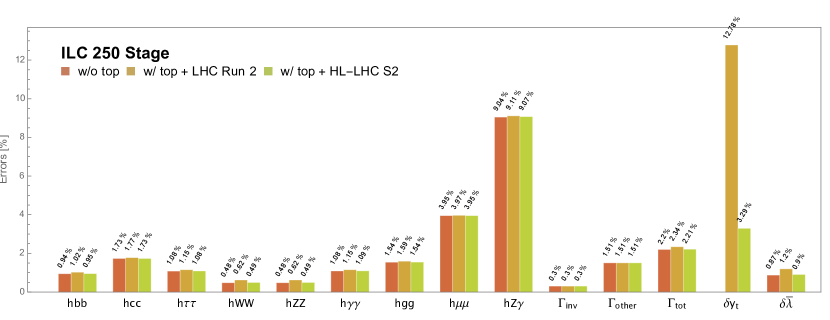
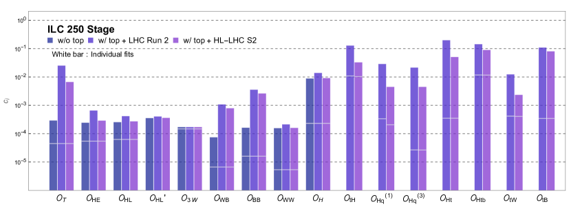
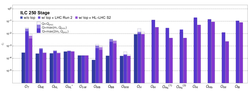
Figure 3: Global fit results for the ILC 250 scenario. The upper panel presents the result in terms of the precision on the physical Higgs couplings (Eq. (3)). The lower panel presents the 1σ1𝜎1\sigma bounds on the operator coefficients, renormalized at Q0=1subscript𝑄01Q_{0}=1 TeV with a suppression scale v𝑣v. RG contributions are evaluated at Q=max(mt,Qproc)𝑄maxsubscript𝑚𝑡subscript𝑄procQ={\rm max}(m_{t},Q_{\rm proc}) as in Eq. (22) and Table 2. In both panels, the first column corresponds to a 22-parameter fit without top operators Barklow:2017suo , used as a reference throughout the paper. The second column presents the result that is obtained when the basis is extended with the seven top operator coefficients described in Section 3.2 and LHC run 2 data are added. The last column repeats the same fit with the expectations of the S2 scenario for the measurement of the top quark electro-weak couplings at HL-LHC. In the bottom panel, white marks are results with only one operator. Results are tabulated in Table 13 and 14.

In this section, we compare several fits on the initial “Higgs factory” stage of the ILC, which collects 2 ab-1 at s=𝑠absent\sqrt{s}= 250 GeV . The benchmark data set for this fit includes the baseline EWPO described in Section 4.1, the measurements of rare Higgs branching ratios at the LHC of Section 4.2 and the ILC Higgs/EW data of Section 4.5. The fits on the extended basis include also LHC measurements of the top quark EW couplings, either at the current run 2 precision (Section 4.3) or the projected precision for the full HL-LHC program in scenario S2 (Section 4.4).

The results of these fits are presented in Fig. 3. The upper panel presents the expected precision of the physical Higgs couplings (defined as the 1σ1𝜎1\sigma constraint on the square root of the decay width (Section 3.1); δλ¯𝛿¯𝜆\delta\bar{\lambda} and δyt𝛿subscript𝑦𝑡\delta y_{t} are defined in Eq. (5) and Eq. (10), respectively). The Higgs coupling precision is evaluated at Qproc=mhsubscript𝑄procsubscript𝑚Q_{\rm proc}=m_{h}, and the result is independent of Q0subscript𝑄0Q_{0} (see Appendix D). The lower panel presents the 1σ1𝜎1\sigma bounds on the operator coefficients. The operator coefficients are renormalized at Q0=1subscript𝑄01Q_{0}=1 TeV with a suppression scale v𝑣v.

For each coupling or operator, three results are presented. The result labeled as “w/o top” is intended for reference: it corresponds to the 22-parameter fit of Ref. Barklow:2017suo without top operators 777The relevant typos in Ref. Barklow:2017suo are collected in Appendix A and are corrected in the fit presented in this paper.. The second bar, labeled “w/top + LHC run 2” corresponds to a fit with the complete 29-parameter basis including top operators of Section 3.7. To ensure convergence of the fit, it includes the current LHC run 2 top physics data of Section 4.3; global fits do not converge without top data as too many parameters need to be determined. The last bar, “w/top + HL-LHC S2”, includes the expected improvements in top physics of the HL-LHC scenario “S2” of Section 4.4.

Remarkably, the ILC precision on the physical Higgs couplings remains robust against model-independent top effects. The global fits with 22 parameters (without tops) and 29 parameters (with tops) yield similar precision. The most pronounced deterioration is observed in the hZZ𝑍𝑍hZZ and hWW𝑊𝑊hWW couplings in the “LHC run 2” scenario, where the precision degrades by 0.48% and 0.62%, respectively. The parameter λ¯¯𝜆\bar{\lambda} degrades by 40%. The precision of the Higgs coupling measurements improves again with the inclusion of stronger top production data from HL-LHC, almost to the level without top effects.

The robustness of the bounds on the physical Higgs couplings is understood as follows. The renormalization scale Q=max(mt,Qproc)𝑄maxsubscript𝑚𝑡subscript𝑄procQ={\rm max}(m_{t},Q_{\rm proc}) for top-loop effects is mtsubscript𝑚𝑡m_{t} for many observables, including Higgs decay widths with Qproc=mh<mtsubscript𝑄procsubscript𝑚subscript𝑚𝑡Q_{\rm proc}=m_{h}<m_{t} and EWPOs with Qproc=mZ<mtsubscript𝑄procsubscript𝑚𝑍subscript𝑚𝑡Q_{\rm proc}=m_{Z}<m_{t}. Thus, those observables depend on common combinations of Higgs operators and their RG corrections by top operators: c~i(mt)=ci+116π2γijcj(Q0)logmtQ0subscript~𝑐𝑖subscript𝑚𝑡subscript𝑐𝑖116superscript𝜋2subscript𝛾𝑖𝑗subscript𝑐𝑗subscript𝑄0subscript𝑚𝑡subscript𝑄0\tilde{c}_{i}(m_{t})=c_{i}+\frac{1}{16\pi^{2}}\gamma_{ij}c_{j}(Q_{0})\log\frac{m_{t}}{Q_{0}} (Eq. (12)). In the limit where only a single scale Q𝑄Q is relevant, all top effects appear through c~i(Q)subscript~𝑐𝑖𝑄\tilde{c}_{i}(Q) so that one can redefine all Higgs operator coefficients cisubscript𝑐𝑖c_{i} by fixed combinations c~i(Q)subscript~𝑐𝑖𝑄\tilde{c}_{i}(Q). Physical Higgs couplings will then depend only on c~isubscript~𝑐𝑖\tilde{c}_{i} in the same way they depended on cisubscript𝑐𝑖c_{i} in the global fit without top operators. Then the global fit results for physical Higgs couplings with top operators must be equivalent to the one without top operators. If all observables are at similar scales, one expects that the Higgs coupling precision is robust against the extension of the basis with the top operators. In Appendix C, we present fit results for several different choices of the scale Q𝑄Q, corroborating this explanation. In other words, the heaviness of the top quark makes the Higgs coupling precision rather insusceptible to model-independent top effects.

This is remarkable. RG effects are discernible from tree-level effects through the measurements at multiple energy scales because RG effects vary with the energy scale while tree-level effects remain constant. Thus, one may expect that measurements at multiple energy scales are the ones responsible to help achieve high precision in global-fit analyses. However, we just saw a very different conclusion; having many observables with common energy scales actually allows to measure certain combinations of tree-level and RG effects (appearing at the common scale) more precisely. This resulted in the robust Higgs coupling precision at the ILC.

On the other hand, by actually the same reason, the constraints on operator coefficients degrade much more significantly with top effects, as shown in the bottom panel of Fig. 3. In the presence of top operators, it is difficult to constrain individual operators that combine into physical Higgs couplings. But many common scales (that made Higgs coupling precision robust) do bother disentangling tree-level effects of Higgs operators and RG effects of top operators. The degeneracies between them are not well resolved by Higgs+EW data at 250 GeV alone. Only with the higher-precision top production data of the HL-LHC S2 scenario, the degeneracies are reduced and operators are better constrained in the global fit. However, the precision does not fully recover to the level of the reference fit at the ILC 250 stage.

Apparently, the two panels of Fig. 3 would seem to lead to different conclusions. While the physical Higgs couplings are affected by 30% to 40% at most, the bounds on operator coefficients can degrade by orders of magnitudes. The projection onto the physical Higgs couplings can be useful because they are robustly and semi-directly measured and theoretical predictions of Higgs coupling deviations in various new physics models are available. But these are not full information of new physics effects. The projection onto the operator constraints is still needed to pinpoint the origin of the deviations and to distinguish new physics models.

Lastly, we discuss one feature shown in Fig. 3. The Higgs couplings that seem to be most sensitive to top effects are g(hWW),g(hZZ)𝑔𝑊𝑊𝑔𝑍𝑍g(hWW),g(hZZ) and λ¯¯𝜆\bar{\lambda}, as shown in the second bars. This is related to the worsening of cT,WB,BBsubscript𝑐𝑇𝑊𝐵𝐵𝐵c_{T,WB,BB} constraints, as shown in the bottom panel. Why are these operators particularly sensitive to top effects? cTsubscript𝑐𝑇c_{T} RG mixes most strongly with top operators, in particular with cHtsubscript𝑐𝐻𝑡c_{Ht}888cHq(1)superscriptsubscript𝑐𝐻𝑞1c_{Hq}^{(1)} also RG mixes, but it is better constrained than cHtsubscript𝑐𝐻𝑡c_{Ht} (Fig. 3) by bb¯𝑏¯𝑏b\bar{b} observables at LEP and LHC Durieux:2019rbz ., and cWB,BBsubscript𝑐𝑊𝐵𝐵𝐵c_{WB,BB} strongly with ctBsubscript𝑐𝑡𝐵c_{tB}999ctWsubscript𝑐𝑡𝑊c_{tW} is better constrained than ctBsubscript𝑐𝑡𝐵c_{tB} by top-decay and single-top measurements at LHC Durieux:2019rbz . It is also why cWWsubscript𝑐𝑊𝑊c_{WW} (mixing with ctWsubscript𝑐𝑡𝑊c_{tW} but not with ctBsubscript𝑐𝑡𝐵c_{tB}) is not degraded as much as cWB,BBsubscript𝑐𝑊𝐵𝐵𝐵c_{WB,\,BB}.. These top operators are also not well constrained.

All in all, the ILC precision of the physical Higgs couplings are remarkably robust against the presence of poorly constrained top operators that affect the Higgs measurements through top-loop effects. However, even if the physical couplings of the Higgs boson are well constrained, strong degeneracies or “blind directions” may be present in the basis of operator coefficients that prevent an unambiguous new physics interpretation of the result. Therefore, precise measurements of the top-quark EW couplings are important to take full advantage of the ILC Higgs factory stage.

5.3 The role of beam polarization

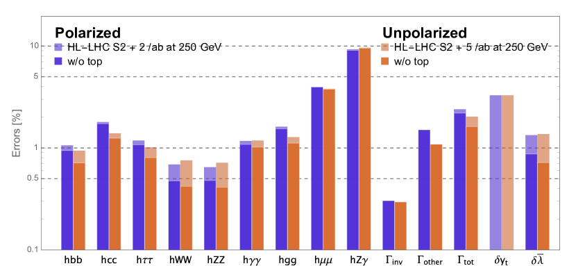
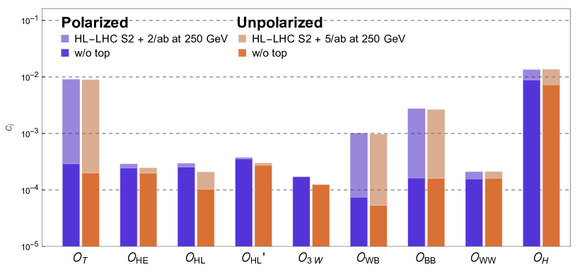
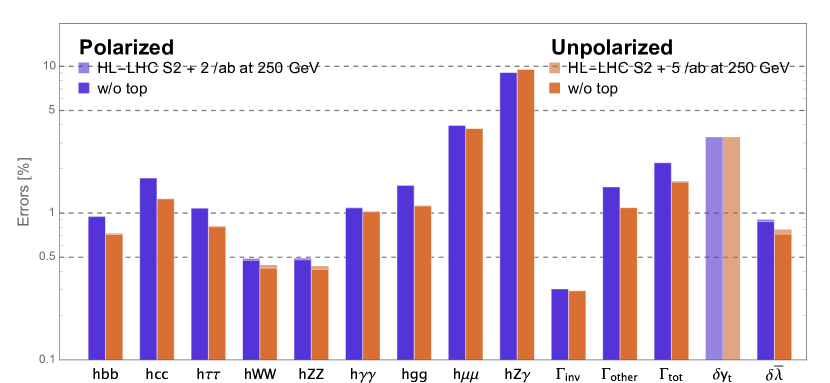
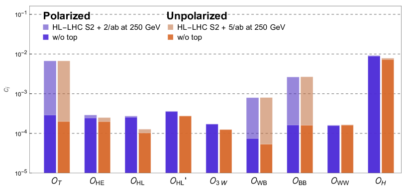
The possibility of highly polarized beams is one of the distinguishing features of linear colliders. It is instructive to compare the impact of top operators on the model-independent precision measurements with and without beam polarization. The one with polarization represents linear e+esuperscript𝑒superscript𝑒e^{+}e^{-} colliders while the other represents circular e+esuperscript𝑒superscript𝑒e^{+}e^{-} colliders. Following Ref. Barklow:2017suo , we compare those results in Fig. 4. The results labeled “polarized” are for the ILC 250 benchmark scenario of Fig. 3, consisting of 1 ab-1 for each of the two beam polarizations; the results labeled “unpolarized” include Higgs measurements in 5 ab-1 without beam polarization and the improved Tera-Z𝑍Z estimates for the Z𝑍Z-pole EWPO (as described in Section 4.1). The light and dark shadings represent the results with and without top operators. In the 29-parameter fit with top operators, HL-LHC S2 top production is included for both polarized and unpolarized scenarios.

As shown in the figure, the power of beam polarization is not significant in terms of the robustness against top effects. The Higgs coupling precisions are all robust irrespective of the existence of beam polarization, as expected from the discussion in Section 5.2. The operator constraints are slightly more robust in the polarized scenario, but the difference is not large. As an interesting remark, the polarization effects become more pronounced if we had used Q=Qproc𝑄subscript𝑄procQ=Q_{\rm proc}, where more various scales are involved; see Appendix C. The beam polarization effectively doubles the number of independent observables, which allows to better disentangle top and Higgs contributions.
Refer to caption
Refer to caption
Figure 4: The role of beam polarization at s=250𝑠250\sqrt{s}=250 GeV on the Higgs coupling precision (upper) and Higgs operator constraints (lower) with (light shading) and without (dark shading) top effects. The polarized (blue) dataset includes equal sharing of two opposite beam polarizaitons (1 ab-1 each) of ILC, and the unpolarized (red) includes a higher luminosity of 5 ab-1 and enhanced Tera-Z𝑍Z precision for EWPO. HL-LHC S2 top data is added.

5.4 The role of electro-weak measurements

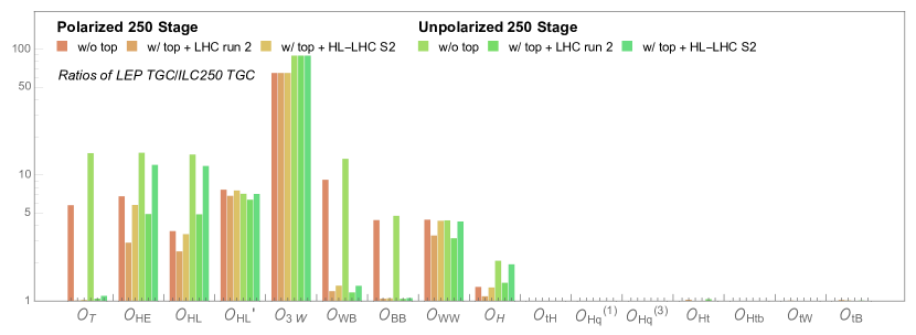
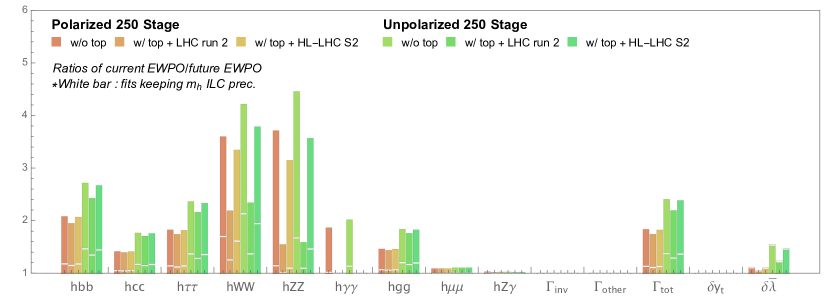
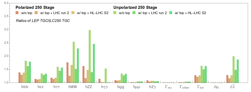
In Fig. 5 we assess the importance of the EWPO and TGC datasets in the global fit by varying the precisions of EWPO and TGC measurements. The height of the bars indicates the ratio of the bounds obtained with the current LEP/SLD precision and with future precisions of ILC250 (except Tera-Z𝑍Z for unpolarized EWPO). Thus, the bars show improvements of global-fit results obtained from the improvement of EW dataset. The exact dataset values used are collected in Table 3. The three bars show different global fits: the first on the reference fit without top operators, and the last two on the fits with top operators including either current LHC run 2 or future HL-LHC S2 bounds on top EW couplings.

The EW measurements generally become less powerful in the presence of top operators in particular when the top operators are relatively not well constrained at LHC run 2; this can be seen as much smaller heights of the second bars. The degeneracies between Higgs and top effects are one of the bottlenecks for taking advantage of the EW precision measurements. As the degeneracies can be reduced by tighter constraints on the top operators from HL-LHC, the importance of EW/TGC dataset also increases. This means that top data and EW/TGC data are complementary or somewhat orthogonal in resolving those degeneracies; but EWPO and TGC alone are not powerful enough to remove those degeneracies. The EW measurements are more important for unpolarized lepton colliders as beam polarization doubles the independent set of observables. The importance is also more pronounced on operator constraints since EW/TGC dataset can directly constrain some operators and reduce degeneracies between operators.

Among all EW observables, the Higgs mass is the most influential one in global fits. White markers indicate the results that are obtained with δmh𝛿subscript𝑚\delta m_{h} fixed to the future LHC/ILC precision of 15 MeV, while all other EWPO continue to vary. These results show that most of the precision improvement from EWPO comes from the improvement of δmh𝛿subscript𝑚\delta m_{h}. This is in agreement with Ref. Lepage:2014fla that did not even consider top effects, implying that the Higgs mass is most important regardless of model-independent top effects. Finally, the further improvement of δmh𝛿subscript𝑚\delta m_{h} from the 15 MeV does not bring additional improvements of global fits at ILC 250.

In summary, the improvements of EW/TGC dataset from the current LEP/SLD precision to the future LHC/ILC precision are very important for the global fits, as well as strong bounds on the top-quark electro-weak operators.
Refer to caption
Refer to caption
Refer to caption
Figure 5: The ratio of Higgs coupling precision obtained by varying EWPO and TGC uncertainties, from current LEP/SLD uncertainties of EWPO (upper panel) and TGC measurements (central panel) to the future uncertainties of ILC250 (Tera-Z𝑍Z for unpolarized EWPO). The white markers indicate the results with the uncertainty δmh𝛿subscript𝑚\delta m_{h} fixed to the future LHC/ILC precision of 15 MeV while all other EWPO uncertainties varied. The third panel presents the results of the variation of the TGC precision in the operator basis. The first three columns are with polarized dataset, and the last three are with unpolarized.

5.5 Results for higher-energy operation – ILC 500 stage

The nominal ILC programme includes 2 ab-1 at s=𝑠absent\sqrt{s}= 250 GeV and 4 ab-1 at s=𝑠absent\sqrt{s}= 500 GeV . The Higgs measurements at higher energy, with much more abundant VBF production, lead to a significantly improved Higgs fit Barklow:2017awn . The sensitivity of measurements in e+eW+Wsuperscript𝑒superscript𝑒superscript𝑊superscript𝑊e^{+}e^{-}\to W^{+}W^{-} increases with center-of-mass energy. And, finally, the high-energy run opens up top quark pair production, allowing for a precise characterization of the electro-weak interactions of the top quark Durieux:2019rbz ; Durieux:2018tev ; Amjad:2015mma .

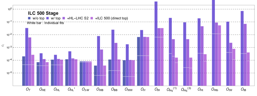
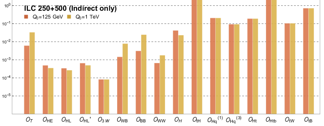
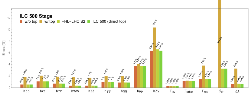
The results of a fit to the combined ILC250+ILC500 scenario are presented in Fig. 6. The upper and lower panels again correspond to the physical Higgs coupling basis and the effective operator coefficients. For each coupling precision and operator constraint, four results are shown. The first bar corresponds to the 22-parameter reference fit to the two ILC stages of Ref Barklow:2017suo . The second, third and fourth bar are obtained with the full 29-parameter basis. The second bar uses only Higgs and EW observables, the third adds the HL-LHC top constraints in the S2 scenario, and the fourth adds the constraints on top EW operators from the ILC run at s=𝑠absent\sqrt{s}= 500 GeV .

Notably, global fits in the 29-parameter basis now converge without top production data (second bar). The dataset with two ILC energy stages provides a sufficiently rich set of measurements to constrain also the top operator coefficients. However, the Higgs coupling precision in this case is significantly degraded with respect to the reference fit, and indirect constraints on top operators remain much worse than those from measurement in top production. Higgs coupling precision without top production data is not as robust as in ILC250 since ILC500 now provides a new energy scale so that the degeneracies with top effects become more important. Adding ILC 500 top production data (fourth bar) can almost fully recover the Higgs coupling precision. HL-LHC top data is also useful, but not quite sufficient to restore the precision to that of the reference fit without top operators.

A more remarkable impact is found in the basis of operator coefficients. In particular, the coefficients cHt,tBsubscript𝑐𝐻𝑡𝑡𝐵c_{Ht,\,tB} and cT,WB,BBsubscript𝑐𝑇𝑊𝐵𝐵𝐵c_{T,\,WB,\,BB}, which mix strongly with each other, are strongly affected. The mixing consequently affects the precision of λ𝜆\lambda and g(hZγ)𝑔𝑍𝛾g(hZ\gamma) too. Only in the last scenario, including ILC 500 top data, the degeneracies between Higgs and top operators are fully resolved and all operators and couplings are constrained as well as in the reference fit without top operators.

All in all, ILC 500 is capable of precise and the model-independent test of the SMEFT with top effects. The precision of the top electro-weak coupling measurements at the HL-LHC and in e+ett¯superscript𝑒superscript𝑒𝑡¯𝑡e^{+}e^{-}\rightarrow t\bar{t} is essential for model-independent Higgs coupling precision.
Refer to caption
Refer to caption
Figure 6: Global-fit results for the ILC250+ILC500 scenario. The upper panel presents the result in terms of the precision on the physical Higgs couplings. The lower panel presents the 1σ1𝜎1\sigma bounds on the operator coefficients, renormalized at Q0=1subscript𝑄01Q_{0}=1 TeV with a suppression scale v𝑣v. In both panels, the first column corresponds to a 22-parameter fit without top operators, that is used as a reference throughout the paper. The second column presents the result that is obtained when the basis is extended with the seven top operator coefficients described in Section 3.2. In the third column, LHC run 2 top data are added. In the fourth column, ILC top measurements at s=𝑠absent\sqrt{s}= 500 GeV are added. In the bottom panel, white marks are results with only one operator. Results are tabulated in Table 13 and 14.

5.6 The Higgs self-coupling

The triple coupling or self-coupling of the Higgs boson is one of the key objectives of high-energy physics in the next decades DiMicco:2019ngk . A robust extraction of this parameter is an important consideration in the design of the Higgs factory and its operating scenarios deBlas:2019wgy ; deBlas:2019rxi ; Barklow:2017awn ; DiVita:2017vrr .

The Higgs self-coupling λ𝜆\lambda and the operator coefficient c6subscript𝑐6c_{6} are expected to be measured in di-Higgs boson production at the LHC before the ILC turns on DiMicco:2019ngk . However, a model-independent extraction from LHC data is difficult. One of the most challenging aspects is that the gghh𝑔𝑔gg\to hh process receives contributions from several diagrams. In addition to the diagram with a triple-Higgs-boson vertex, box and loop diagrams involving tt¯h𝑡¯𝑡t\bar{t}h vertices yield sizeable contributions to the total rate. This results in a strong dependence on several operator coefficients, among which ctHsubscript𝑐𝑡𝐻c_{tH} Azatov:2015oxa .

 (δσ(Zhh))21/2superscriptdelimited-⟨⟩superscript𝛿𝜎𝑍212\left<(\delta\sigma(Zhh))^{2}\right>^{1/2}
w/o top op. ILC 250 2.66%
ILC 250 + 500 2.13%
w/top op. ILC 250 + 500 (Higgs/EW) 8.06%
+ HL-LHC top 2.62%
+ ILC 500 top 2.13%
Table 4: Total uncertainties of the σ(Zhh)𝜎𝑍\sigma(Zhh) contributed from EFT operators, evaluated at Q=500𝑄500Q=500 GeV. Measurement uncertainties are estimated to be 16% Duerig:2016dvi ; Bambade:2019fyw but not shown. These results are independent on Q0subscript𝑄0Q_{0} (Appendix D). The first two rows correspond to the fit on the 22-parameter basis without top operators, for ILC Higgs/EW data at s=𝑠absent\sqrt{s}= 250 GeV and for the complete programme at 250 + 500 GeV . The three last rows correspond to the 29-parameter fit on the complete basis with top operators. The first of them includes Higgs/EW data only, while the second and third add top physics measurements at the HL-LHC and ILC500, respectively.

In our EFT fit, as discussed at the end of Section 3.4, the Higgs self-coupling λ𝜆\lambda and c6subscript𝑐6c_{6} appear together in the λ¯¯𝜆\bar{\lambda} parameter (Eq. (5)), which is constrained by measurement of the Higgs mass. Figure 6 shows that the reference result δλ¯=𝛿¯𝜆absent\delta\bar{\lambda}= 0.66% of the 22-parameter fit at ILC500 is degraded to 3.29% when the basis is extended with top operators. The precision recovers to 0.68% after inclusion of HL-LHC top data in the S2 scenario, and fully recovers with the top measurements in e+ett¯superscript𝑒superscript𝑒𝑡¯𝑡e^{+}e^{-}\to t\bar{t} production at ILC500.

Even if the λ¯¯𝜆\bar{\lambda} coefficient is tightly bounded, we cannot constrain λ𝜆\lambda and c6subscript𝑐6c_{6} individually with the 250 GeV data alone (remember that finite loop effects from the Higgs operator on the Zh𝑍Zh cross section are not included in the fit). The coefficients c6subscript𝑐6c_{6} is precisely measured by σ(Zhh)𝜎𝑍\sigma(Zhh) at ILC500. This measurement separates the two parameters, since λ𝜆\lambda and c6subscript𝑐6c_{6} enter in different combinations in that process. Here, we evaluate the effect of Higgs and top operator coefficients on the extraction of c6subscript𝑐6c_{6}.

Table 4 shows the total uncertainty on the cross-section δσ(Zhh)𝛿𝜎𝑍\delta\sigma(Zhh) from EFT coefficients. This EFT error contribution in the model-independent extraction of c6subscript𝑐6c_{6} must be kept small - by precise measurements of single-Higgs and top production rates - to convincingly attribute a measured deviation in the double Higgs production cross section to a shift in the triple Higgs coupling. The errors are evaluated at Q=500𝑄500Q=500 GeV, and the results are independent of the choice Q0subscript𝑄0Q_{0}.

With only Higgs+EW data, the EFT uncertainty contribution is 8.06%, better than the expected measurement error of 16% Duerig:2016dvi ; Bambade:2019fyw . This means that the measurement of c6subscript𝑐6c_{6} from σ(e+eZhh)𝜎superscript𝑒superscript𝑒𝑍\sigma(e^{+}e^{-}\to Zhh) is robust, even in the presence of top operators. Addition of the HL-LHC top production data improves the uncertainty to 2.6%. Finally, e+ett¯superscript𝑒superscript𝑒𝑡¯𝑡e^{+}e^{-}\to t\bar{t} at s=𝑠absent\sqrt{s}= 500 GeV fully recovers the constraint 2.13% of the reference fit without top operators.

An interesting aside is that, even though the final errors are 2.13% both with or without top operators, individual EFT contributions to the total error are quite different. In the fit on the extended basis, cTsubscript𝑐𝑇c_{T} becomes the dominant source of EFT uncertainties while cHsubscript𝑐𝐻c_{H} was the dominant contribution before top operators were added.

In summary, the extraction of the Higgs boson self-coupling from the di-Higgs production rate at the ILC at s=𝑠absent\sqrt{s}= 500 GeV is robust against the impact of other Higgs operators and top operators. With the inclusion of HL-LHC and ILC500 results on top electro-weak couplings, the effect of those operators on the extraction is reduced to well below the expected measurement uncertainty.

5.7 Indirect bounds on top-EW couplings
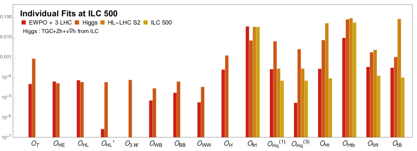
Refer to caption
Figure 7: The individual constraints on the EFT coefficients by each set of measurements at ILC 500 and HL-LHC stages. The first column (EWPO+3 LHC) shows the individual bounds by 9 EWPOs and 3 branching ratios measurements from LHC. The second column (Higgs) is from the TGC measurements and Higgs production processes (Zh+νν¯h𝑍𝜈¯𝜈Zh\,+\,\nu\bar{\nu}h) from ILC. The third and fourth ones represent those from direct top data of HL-LHC and ILC 500-top respectively.

The effect of the top operator coefficients on the Higgs and EW observables offers a way to probe these operators during the first “Higgs factory” stage of the ILC project at s=𝑠absent\sqrt{s}= 250 GeV, when the top quark pair production process is not yet accessible. The indirect bound from the Higgs/EW fit is therefore the first top quark physics of the new project.

The individual bounds on all operator coefficients from a fit to the ILC500 projection are presented in Fig. 7. The measurements are grouped in two broad categories: electro-weak precision measurements and Higgs coupling measurements. These indirect determinations are compared to the projections for HL-LHC top physics results in the S2 scenario and to the bounds expected from ILC top measurements at s=𝑠absent\sqrt{s}= 500 GeV .

The Higgs/EW precision data at s=𝑠absent\sqrt{s}= 250 GeV are sensitive to the top electro-weak couplings through loop effects. The complete set of relations is found in Table 11. The Higgs decay widths Γ(hγγ)Γ𝛾𝛾\Gamma(h\rightarrow\gamma\gamma) and Γ(hZγ)Γ𝑍𝛾\Gamma(h\rightarrow Z\gamma) are particularly sensitive to the dipole operator coefficients ctWsubscript𝑐𝑡𝑊c_{tW} and ctBsubscript𝑐𝑡𝐵c_{tB} that affect the Ztt¯𝑍𝑡¯𝑡Zt\bar{t} and γtt¯𝛾𝑡¯𝑡\gamma t\bar{t} vertices and to the top-quark Yukawa coupling and hence CtHsubscript𝐶𝑡𝐻C_{tH}. Figure 3 and 6 show that the ILC precision can measure these widths to 𝒪(1)%𝒪percent1{\cal O}(1)\% precision. In Fig. 7 the individual bounds from Higgs measurements are indicated as the second, orange bar. The indirect bounds from Higgs observables are indeed found to be quite powerful for a number of operators. The individual bounds on cHtsubscript𝑐𝐻𝑡c_{Ht}, ctHsubscript𝑐𝑡𝐻c_{tH} and, especially ctBsubscript𝑐𝑡𝐵c_{tB} are expected to improve the bounds from the HL-LHC measurements by one to two orders of magnitude.

Also the electro-weak precision measurements, indicated with the first, red bar in Fig. 7, offer very good sensitivity. Renormalization-group mixing leads to a dependence of the electro-weak precision observables on top operators. Most individual bounds on top operator coefficients exceed the S2 projection for the HL-LHC, and in several cases (cHq(3)superscriptsubscript𝑐𝐻𝑞3c_{Hq}^{(3)}, cHtsubscript𝑐𝐻𝑡c_{Ht}, ctBsubscript𝑐𝑡𝐵c_{tB}) by more than two orders of magnitude. In some cases, these individual bounds are competitive even when compared to the limits from direct e+ett¯superscript𝑒superscript𝑒𝑡¯𝑡e^{+}e^{-}\rightarrow t\bar{t} production in the 500 GeV run.

The Higgs and electro-weak measurements at s=𝑠absent\sqrt{s}= 250 GeV therefore provide a powerful indirect handle on the top electro-weak couplings and can improve the legacy bounds from the LHC top physics programme. If these couplings receive corrections from new physics, the Higgs/EW measurements may well be the first place where significant deviations from the SM show up. We find, however, that these individual bounds are generally not robust and an unambiguous determination of the coefficients in a global fit requires the inclusion of e+ett¯superscript𝑒superscript𝑒𝑡¯𝑡e^{+}e^{-}\rightarrow t\bar{t} data at higher energy. The bound on the dipole operator ctBsubscript𝑐𝑡𝐵c_{tB} is the only case, where the addition of the Higgs/EW data improves the global limit over the result of a fit to HL-LHC top physics data. For this operator a weak sensitivity of rare associated production processes (pptt¯γ𝑝𝑝𝑡¯𝑡𝛾pp\rightarrow t\bar{t}\gamma, pptt¯Z𝑝𝑝𝑡¯𝑡𝑍pp\rightarrow t\bar{t}Z, pptZq𝑝𝑝𝑡𝑍𝑞pp\to tZq) at the HL-LHC coincides with a relatively strong sensitivity of the Higgs/EW observables.

5.8 The top-quark Yukawa coupling

The top-quark Yukawa coupling is an important parameter of the SM and merits a dedicated discussion.

The indirect sensitivity to ctHsubscript𝑐𝑡𝐻c_{tH} stems from loop-induced Higgs boson decay widths Γ(hγγ)Γ𝛾𝛾\Gamma(h\rightarrow\gamma\gamma), Γ(hZγ)Γ𝑍𝛾\Gamma(h\rightarrow Z\gamma) and Γ(hgg)Γ𝑔𝑔\Gamma(h\rightarrow gg) that involve top-quark loops. No other observables in Table 11 depend on ctHsubscript𝑐𝑡𝐻c_{tH}. In Fig. 7 the indirect bound on ctHsubscript𝑐𝑡𝐻c_{tH} from the ILC Higgs data is much more stringent than the direct measurement in pptt¯H𝑝𝑝𝑡¯𝑡𝐻pp\rightarrow t\bar{t}H at the HL-LHC. This finding confirms the good indirect sensitivity to the Yukawa coupling found by Ref. Boselli:2018zxr .

However, as for the other top operators, the excellent individual bounds do not translate into a robust measurement of the top-quark Yukawa coupling. The top-quark Yukawa contributions to the Higgs decay widths are entangled with other contributions. The degeneracy between the different operator coefficients cannot be lifted with Higgs and electro-weak data alone. Indeed, the global bound on the top Yukawa in a model-independent fit is entirely dominated by the direct measurements in tt¯H𝑡¯𝑡𝐻t\bar{t}H production.

Before proceeding to discuss the direct measurements, we explore possible improvements in the indirect constraints on top Yukawa. First, Γ(hgg)Γ𝑔𝑔\Gamma(h\rightarrow gg) was identified as the most promising indirect constraint in Ref. Boselli:2018zxr . In addition to ctHsubscript𝑐𝑡𝐻c_{tH}, Γ(hgg)Γ𝑔𝑔\Gamma(h\to gg) receives contributions from ctGsubscript𝑐𝑡𝐺c_{tG} and hgg𝑔𝑔hgg contact operators. Although the former is likely well constrained by the measurements of the top quark pair production cross section at hadron colliders with a global limit -0.4 <ctG/Λ2<absentsubscript𝑐𝑡𝐺superscriptΛ2absent<c_{tG}/\Lambda^{2}< 0.4 Hartland:2019bjb , the degeneracy with the hgg𝑔𝑔hgg operator is very hard to lift Azatov:2016xik . On the other hand, for Γ(hγγ)Γ𝛾𝛾\Gamma(h\to\gamma\gamma) and Γ(hZγ)Γ𝑍𝛾\Gamma(h\to Z\gamma), ctHsubscript𝑐𝑡𝐻c_{tH} must be separated from ctW,tBsubscript𝑐𝑡𝑊𝑡𝐵c_{tW,tB} as well as cWB,BBsubscript𝑐𝑊𝐵𝐵𝐵c_{WB,BB}. These operators can perhaps be better constrained if differential analyses of tt¯X𝑡¯𝑡𝑋t\bar{t}X production at the LHC can improve the bounds significantly over the precision envisaged S2 scenario.

The direct measurements of the top quark Yukawa coupling have been discussed in some detail in Ref. Fujii:2019zll . The HL-LHC measurements of the tt¯H𝑡¯𝑡𝐻t\bar{t}H cross section yield a precision of 3.29% in our fit101010We note here that, while the extraction of the top Yukawa coupling from the tt¯h𝑡¯𝑡t\bar{t}h cross section is the most robust handle on this coupling, it is by no means immune to degradation due to the presence of other operators, as demonstrated by recent global fits Hartland:2019bjb . Also the claim of Ref. Plehn:2015cta of a 1% precision on the Yukawa coupling from the ratio of the tt¯H𝑡¯𝑡𝐻t\bar{t}H and tt¯Z𝑡¯𝑡𝑍t\bar{t}Z rates must be carefully assessed in a global environment.. The precision can be further improved with tt¯h𝑡¯𝑡t\bar{t}h measurements from ILC runs at high energy. The ILC must be operated at s=𝑠absent\sqrt{s}= 550 GeV to match the 3% precision of the HL-LHC in the direct extraction from the e+ett¯hsuperscript𝑒superscript𝑒𝑡¯𝑡e^{+}e^{-}\to t\bar{t}h channel and confirm a possible deviation from the SM. The operation of a linear collider at 1 TeV can improve the constraint by another factor two. The analysis in Ref. Durieux:2019rbz shows that the extraction from the tt¯h𝑡¯𝑡t\bar{t}h rate at the ILC is robust when data at 1 TeV are added to constrain the coefficients of e+ett¯superscript𝑒superscript𝑒𝑡¯𝑡e^{+}e^{-}t\bar{t} operators in a global fit. The combination of all these measurements will allow to measure top-quark Yukawa coupling with approximately 1% precision.

Finally, we note an interesting direction to constrain ctHsubscript𝑐𝑡𝐻c_{tH}. The operator RG mixes with c6subscript𝑐6c_{6}. But we did not need to include the running of c6subscript𝑐6c_{6} because c6subscript𝑐6c_{6} enters in only one observable σ(Zhh)𝜎𝑍\sigma(Zhh) at s=500𝑠500\sqrt{s}=500 GeV. If finite loop corrections of c6subscript𝑐6c_{6} to σ(Zh)𝜎𝑍\sigma(Zh) at s=250𝑠250\sqrt{s}=250 GeV McCullough:2013rea can be considered in the future, multiple energy scales may yield a new way to constrain the ctHsubscript𝑐𝑡𝐻c_{tH}’s RG contributions. The HL-LHC Higgs pair production DiMicco:2019ngk may even be used too. A more dedicated study is postponed to a future work TianPeskinLambda .

In summary, we confirm the good indirect sensitivity of the 250 GeV run to the top-quark Yukawa coupling that was signalled by Ref. Boselli:2018zxr . The ILC Higgs programme at 250 GeV can provide individual, single-parameter bounds on ctHsubscript𝑐𝑡𝐻c_{tH} that are more stringent than those from the HL-LHC. Hence, the ILC initial stage may observe strong deviations from the Standard Model predictions in the Hγγ𝐻𝛾𝛾H\rightarrow\gamma\gamma and Hgg𝐻𝑔𝑔H\rightarrow gg decay rates, should the top-quark Yukawa coupling be affected by physics beyond the Standard Model. However, we find that the indirect extraction of ctHsubscript𝑐𝑡𝐻c_{tH} from the Higgs branching ratios is not robust in a global fit. This means that a deviation from the SM cannot unambiguously be attributed to ctHsubscript𝑐𝑡𝐻c_{tH}; the effect could be caused by another operator. To pinpoint the new physics effect, a measurement of the associated production rate of a Higgs boson with a top quark pair at higher energy remains necessary.

6 Summary

In this paper, we have presented a global SMEFT fit for the ILC by combining contributions from Higgs/EW and top sectors. In addition to the 22 parameters of Higgs operators and SM parameters which are complete at the lowest order Barklow:2017suo ; deBlas:2019rxi , this requires seven top-quark operators. They contribute to the Higgs/EW precision observables at the one-loop suppressed order compared to those of Higgs operators (except for tree-level shifts of tt¯h𝑡¯𝑡t\bar{t}h and tt¯Z𝑡¯𝑡𝑍t\bar{t}Z couplings), but they are leading contributions of top operators. The 29-parameter fit then provides a complete and model-independent description of leading Higgs+EW+top effects on precision observables at future lepton colliders.

The loop calculations of top effects necessarily introduce new uncertainties. The top-loop contributions were included through the renormalization mixing with Higgs operators. Although good proxies of full one-loop effects, the RG contributions are only a subset of the full one-loop results111111 While including full one-loop effects for all the relevant observables is beyond the scope of this paper, we recognize that the important effect from the left-over finite contributions would be mainly coming from ctBsubscript𝑐𝑡𝐵c_{tB} term in Γ(hγγ)Γ𝛾𝛾\Gamma(h\to\gamma\gamma), provided the prospected constraints on top operators from HL-LHC; see details in Appendix B.2.. The impact of RG effects depend on the renormalization scale Q𝑄Q to which the Higgs operators will run from a common scale Q0subscript𝑄0Q_{0} where all the operators are defined. Q=max(mt,Qproc)𝑄maxsubscript𝑚𝑡subscript𝑄procQ={\rm max}(m_{t},Q_{\rm proc}) was used as the default choice, but the variations with respect to Q=Qproc𝑄subscript𝑄procQ=Q_{\rm proc} and max(2mt,Qproc)max2subscript𝑚𝑡subscript𝑄proc{\rm max}(2m_{t},Q_{\rm proc}) reflect the errors from even higher-order quantum corrections.

With this formalism, we have evaluated the prospects of the ILC in the extended 29-parameter basis, in comparison with those of the previous 22-parameter fit of Ref. Barklow:2017awn . We have found that the Higgs fit at ILC 250 GeV is strongly affected by the inclusion of top effects. This result, and those of Ref. Vryonidou:2018eyv ; Durieux:2018ggn , show that results obtained with today’s state of the art SMEFT fits must be interpreted with care, as they may not hold in a more complete fit121212As a familiar example, one can consider the well-known κ𝜅\kappa-framework to interpret Higgs boson coupling measurements. Clearly, the limitations of the κ𝜅\kappa framework affect the conclusions of a benchmark analysis in important ways: due to the assumptions inherent in the fit, it fails to acknowledge the role of EWPO and beam polarization, to name just two examples. The importance of these aspects becomes apparent only in a more advanced EFT approach..

To mitigate the effect of the additional degrees of freedom, their contribution must be disentangled by including precise measurements of the top quark electro-weak couplings. The precision of the HL-LHC top physics program, as envisaged in the S2 scenario of Ref. Durieux:2019rbz , is sufficient to restore the precision of the physical Higgs boson couplings. But it still leaves several of the underlying EFT operator coefficients relatively poorly constrained. This implies that, even if the Higgs couplings can be precisely determined and their deviations from SM predictions can be well detected, it becomes harder to pinpoint the source of the deviations, should they be observed. The projection of the EFT fit results on the physical Higgs couplings offers a set of bounds with an intuitive physical interpretation, but can obscure potentially very important information. It is therefore important to present both sets of results – Higgs coupling precisions and operator constraints – to fully characterize the analyzing power of the data.

We also assess whether the Higgs/EW precision data in the initial stage at s=𝑠absent\sqrt{s}= 250 GeV can place bounds on top operators before top quark pairs are produced at the ILC. These indirect bounds are very very competitive if only a single top operator is considered in a fit. For example, the hgg𝑔𝑔h\rightarrow gg and hγγ𝛾𝛾h\rightarrow\gamma\gamma decay rates yield indirect sensitivity on the top coupling at sub-% precision, well beyond what can be achieved in associated tt¯h𝑡¯𝑡t\bar{t}h productions in all planned lepton or hadron colliders. However, these individual bounds turn out to be not robust in the presence of other operators with non-zero coefficients. A robust determination of top operators requires the inclusion of e+ett¯superscript𝑒superscript𝑒𝑡¯𝑡e^{+}e^{-}\rightarrow t\bar{t} and e+ett¯hsuperscript𝑒superscript𝑒𝑡¯𝑡e^{+}e^{-}\to t\bar{t}h data at higher center-of-mass energy.

In the complete ILC programme, with a second energy stage at 500 GeV, a precise characterization of the e+ett¯superscript𝑒superscript𝑒𝑡¯𝑡e^{+}e^{-}\rightarrow t\bar{t} process provides very precise constraints on the top operators. A combined fit on Higgs, EW and top quark precision data then over-constrains the EFT fit, yielding robust bounds on all 29 operators and the unambiguous identification of the origin of any deviations from the SM.

Acknowledgements.
This work builds on the effort of the LHC collaborations and the ILC and CLIC simulation studies. We would like to acknowledge the work of our colleagues in this place. We owe special thanks to Gauthier Durieux, Michael Peskin and Cen Zhang for their feedback on the project and write-up. SJ and JL are supported by Grant Korea NRF-2019R1C1C1010050, 2017R1D1A1B03030820, 2015R1A4A1042542, and SJ also by POSCO Science Fellowship. MP and MV are supported by the Spanish national program for particle physics, projects FPA2015-65652-C4-3-R (MINECO/FEDER) and PGC2018-094856-B-100, and PROMETEO grant 2018/060 of the Generalitat Valenciana. MP is supported by the “Severo Ochoa” Grant SEV-2014-0398-05, reference BES-2015-072974. JT was supported by the Japan Society for the Promotion of Science (JSPS) under Grants-in-Aid for Science Research 15H02083.

Appendix A Typos and corrections in Ref.Barklow:2017awn

Ref. Barklow:2017awn ; Barklow:2017suo and the distributed C++ code, on which our study is based, contain several mild typos and mistakes. We collect them in this appendix using the same notation, and we make the corrected Mathematica code available upon request.

  1. 1.

    Typos in the paper Barklow:2017awn :

    1. (a)

      Some expressions for the TGCs written in the Section 3 and Appendix of Ref. Barklow:2017awn should be corrected in a right form. The amplitudes of eR,LeL,R+WL+WLsuperscriptsubscript𝑒𝑅𝐿superscriptsubscript𝑒𝐿𝑅superscriptsubscript𝑊𝐿superscriptsubscript𝑊𝐿e_{R,L}^{-}e_{L,R}^{+}\to W_{L}^{+}W_{L}^{-} are

      𝒜Rsubscript𝒜𝑅\displaystyle\mathcal{A}_{R} =\displaystyle= e2κAgRgZκZ,superscript𝑒2subscript𝜅𝐴subscript𝑔𝑅subscript𝑔𝑍subscript𝜅𝑍\displaystyle e^{2}\kappa_{A}\,-\,g_{R}g_{Z}\kappa_{Z}, (36)
      𝒜Lsubscript𝒜𝐿\displaystyle\mathcal{A}_{L} =\displaystyle= e2κAgLgZκZgW22.superscript𝑒2subscript𝜅𝐴subscript𝑔𝐿subscript𝑔𝑍subscript𝜅𝑍superscriptsubscript𝑔𝑊22\displaystyle e^{2}\kappa_{A}\,-\,g_{L}g_{Z}\kappa_{Z}-\frac{g_{W}^{2}}{2}. (37)

      The κVsubscript𝜅𝑉\kappa_{V} denote the deviation of the triple gauge couplings between W+Wsuperscript𝑊superscript𝑊W^{+}W^{-} and V(=Z,A)V(=Z,A). The gWsubscript𝑔𝑊g_{W} is the W boson coupling to leptons(electron and neutrino) that is introduced only to the amplitude for eLeR+superscriptsubscript𝑒𝐿superscriptsubscript𝑒𝑅e_{L}^{-}e_{R}^{+} through the neutrino exchange diagram. In the Ref. Barklow:2017awn , the sign of the terms for gL(gR)gZκZsubscript𝑔𝐿subscript𝑔𝑅subscript𝑔𝑍subscript𝜅𝑍g_{L}(g_{R})g_{Z}\kappa_{Z} is written as plus but the negative one is correct. The fits were done with the correct sign but one term for δe𝛿𝑒\delta e in δgZ,eff𝛿subscript𝑔𝑍𝑒𝑓𝑓\delta g_{Z,eff} was missed. By the definition of the effective TGC (Barklow:2017awn ),

      δgZ,eff=1gcw2(2Δ𝒜LΔ𝒜R),𝛿subscript𝑔𝑍𝑒𝑓𝑓1𝑔superscriptsubscript𝑐𝑤22Δsubscript𝒜𝐿Δsubscript𝒜𝑅\delta g_{Z,eff}=\frac{1}{gc_{w}^{2}}\left(2\Delta\mathcal{A}_{L}-\Delta\mathcal{A}_{R}\right), (38)

      the δgZ,eff𝛿subscript𝑔𝑍𝑒𝑓𝑓\delta g_{Z,eff} has one more term which was missed and we find

      δgZ,eff=δgZ+1cw2((cw2sw2)δgL+sw2δgR 2δgW+ 2sw2δe).𝛿subscript𝑔𝑍𝑒𝑓𝑓𝛿subscript𝑔𝑍1superscriptsubscript𝑐𝑤2superscriptsubscript𝑐𝑤2superscriptsubscript𝑠𝑤2𝛿subscript𝑔𝐿superscriptsubscript𝑠𝑤2𝛿subscript𝑔𝑅2𝛿subscript𝑔𝑊2superscriptsubscript𝑠𝑤2𝛿𝑒\delta g_{Z,eff}\,=\,\delta g_{Z}\,+\,\frac{1}{c_{w}^{2}}((c_{w}^{2}-s_{w}^{2})\delta g_{L}\,+\,s_{w}^{2}\delta g_{R}\,-\,2\delta g_{W}\,+\,2s_{w}^{2}\delta e). (39)

      This can be checked using the fact that the TGCs are independent of cWB,BB,WWsubscript𝑐𝑊𝐵𝐵𝐵𝑊𝑊c_{WB,BB,WW} because the Δ𝒜R,LΔsubscript𝒜𝑅𝐿\Delta\mathcal{A}_{R,L} are also independent of them.

  2. 2.

    Typos in the code distributed with Barklow:2017awn :

    1. (a)

      δgR=cw2δg+(1+cw2)δg12sw2cHE12cw2(8cWW)+cw2(8cWB)+12sw2cw2(1+cw2)(8cBB)𝛿subscript𝑔𝑅superscriptsubscript𝑐𝑤2𝛿𝑔1superscriptsubscript𝑐𝑤2𝛿superscript𝑔12superscriptsubscript𝑠𝑤2subscript𝑐𝐻𝐸12superscriptsubscript𝑐𝑤28subscript𝑐𝑊𝑊superscriptsubscript𝑐𝑤28subscript𝑐𝑊𝐵12superscriptsubscript𝑠𝑤2superscriptsubscript𝑐𝑤21superscriptsubscript𝑐𝑤28subscript𝑐𝐵𝐵\delta g_{R}\,=\,-c_{w}^{2}\delta g+(1+c_{w}^{2})\delta g^{\prime}-\frac{1}{2s_{w}^{2}}c_{HE}-\frac{1}{2}c_{w}^{2}(8c_{WW})+c_{w}^{2}(8c_{WB})+\frac{1}{2}\frac{s_{w}^{2}}{c_{w}^{2}}(1+c_{w}^{2})(8c_{BB}) : the sign of the (8cWW)8subscript𝑐𝑊𝑊(8c_{WW}) was reversed.

    2. (b)

      bL=1(12sw2)[cw2(12sw2mZ2s)(8cWW)+2sw2(12sw2)mZ2s(8cWB)sw4cw2(12cw2mZ2s)(8cBB)]subscript𝑏𝐿112superscriptsubscript𝑠𝑤2delimited-[]superscriptsubscript𝑐𝑤212superscriptsubscript𝑠𝑤2superscriptsubscript𝑚𝑍2𝑠8subscript𝑐𝑊𝑊2superscriptsubscript𝑠𝑤212superscriptsubscript𝑠𝑤2superscriptsubscript𝑚𝑍2𝑠8subscript𝑐𝑊𝐵superscriptsubscript𝑠𝑤4superscriptsubscript𝑐𝑤212superscriptsubscript𝑐𝑤2superscriptsubscript𝑚𝑍2𝑠8subscript𝑐𝐵𝐵b_{L}\,=\,\frac{1}{(1-2s_{w}^{2})}\left[c_{w}^{2}(1-2s_{w}^{2}\frac{m_{Z}^{2}}{s})(8c_{WW})+2s_{w}^{2}(1-2s_{w}^{2})\frac{m_{Z}^{2}}{s}(8c_{WB})-\frac{s_{w}^{4}}{c_{w}^{2}}(1-2c_{w}^{2}\frac{m_{Z}^{2}}{s})(8c_{BB})\right]


      : 1cw2(12cw2mZ2s)(8cBB)1superscriptsubscript𝑐𝑤212superscriptsubscript𝑐𝑤2superscriptsubscript𝑚𝑍2𝑠8subscript𝑐𝐵𝐵-\frac{1}{c_{w}^{2}}(1-2c_{w}^{2}\frac{m_{Z}^{2}}{s})(8c_{BB}) was used instead of the above (8cBB)8subscript𝑐𝐵𝐵(8c_{BB}) term.

    3. (c)

      kh=EZmh22k2sEZ2/mZ2(2+EZ2/mZ2)mh2EZssubscript𝑘subscript𝐸𝑍superscriptsubscript𝑚22superscript𝑘2𝑠superscriptsubscript𝐸𝑍2superscriptsubscript𝑚𝑍22superscriptsubscript𝐸𝑍2superscriptsubscript𝑚𝑍2superscriptsubscript𝑚2subscript𝐸𝑍𝑠k_{h}\,=\,-\frac{E_{Z}m_{h}^{2}}{2k^{2}\sqrt{s}}-\frac{E_{Z}^{2}/m_{Z}^{2}}{(2+E_{Z}^{2}/m_{Z}^{2})}\frac{m_{h}^{2}}{E_{Z}\sqrt{s}} in the Zh𝑍Zh measurement.
      : the first term was inserted as EZmZ22k2ssubscript𝐸𝑍superscriptsubscript𝑚𝑍22superscript𝑘2𝑠-\frac{E_{Z}m_{Z}^{2}}{2k^{2}\sqrt{s}}. The Z boson mass was used for the Higgs mass.

    4. (d)

      δσ(R)= 2δgR+1.40ηZ+1.02ηZZ+18.6δZZ28.7δZAZ+0.56ηh+𝛿𝜎𝑅2𝛿subscript𝑔𝑅1.40subscript𝜂𝑍1.02subscript𝜂𝑍𝑍18.6𝛿subscript𝑍𝑍28.7𝛿subscript𝑍𝐴𝑍0.56subscript𝜂\delta\sigma(R)\,=\,2\delta g_{R}+1.40\eta_{Z}+1.02\eta_{ZZ}+18.6\delta Z_{Z}-28.7\delta Z_{AZ}+0.56\eta_{h}+\cdots for the Zhh𝑍Zhh cross section.
      : 2δgL2𝛿subscript𝑔𝐿2\delta g_{L} was used instead of the first term, 2δgR2𝛿subscript𝑔𝑅2\delta g_{R} in the estimate of the uncertainty of σ(Zhh)𝜎𝑍\sigma(Zhh).

    5. (e)

      In the fits for “+Zh𝑍+Zh” columns in Table 5, the aL,aRsubscript𝑎𝐿subscript𝑎𝑅a_{L},\,a_{R} parameters were inserted in the place of bL,bRsubscript𝑏𝐿subscript𝑏𝑅b_{L},\,b_{R} as error inputs of the Zh measurement but in ILC 250,500 fits the error inputs were used correctly.

    6. (f)

      When the total cross section of ee+Zhsuperscript𝑒superscript𝑒𝑍e^{-}e^{+}\to Zh is prepared for the its error estimate in the fits for 250+350 GeV in the fourth column of Table 6, only left-handed one was inserted, that is right-handed one was missing.

By correcting the typos, we re-obtain the Table 2 in Ref. Barklow:2017awn and Table 3 in Barklow:2017suo in Table 5 and 6, respectively. The impact of the typos on the Higgs precision is rather mild while the impact on some operators is significant. Especially, the constraint on cHEsubscript𝑐𝐻𝐸c_{HE} decreases significantly from the “+LHC” column as shown in Table 5 mainly due to item 2a and the difference reduces at the ILC 500 and ILC 250+500 fits where the influence of the LHC Higgs measurements becomes weak relatively. We also found that the missing right-handed σ(Zh)𝜎𝑍\sigma(Zh) part (item 2f) in the 250+350 GeV fit reduces the error of the cross section to the half of the original value as shown in the “+1.5/ab 350 GeV ” column of Table 6.

prec. EW + WW𝑊𝑊WW + LHC + Zh𝑍Zh ILC 250
rep. corr. rep. corr. rep. corr. rep. corr. rep. corr.
cTsubscript𝑐𝑇c_{T} 0.011 0.011 0.051 0.051 0.051 0.051 0.048 0.049 0.052 0.050
cHEsubscript𝑐𝐻𝐸c_{HE} 0.043 0.043 0.026 0.026 0.085 0.026 0.047 0.024 0.055 0.025
cHLsubscript𝑐𝐻𝐿c_{HL} 0.042 0.042 0.035 0.035 0.035 0.035 0.032 0.03 0.039 0.030
cHLsuperscriptsubscript𝑐𝐻𝐿c_{HL}^{\prime} . . 0.028 0.028 0.028 0.028 0.028 0.027 0.047 0.039
8cWB8subscript𝑐𝑊𝐵8\,c_{WB} . . 0.078 0.078 0.080 0.080 0.076 0.078 0.090 0.091
8cBB8subscript𝑐𝐵𝐵8\,c_{BB} . . . . 0.20 0.20 0.16 0.18 0.11 0.17
8cWW8subscript𝑐𝑊𝑊8\,c_{WW} . . . . 0.21 0.21 0.13 0.17 0.13 0.19
8cH8subscript𝑐𝐻8\,c_{H} . . . . . . 1.12 1.12 1.20 0.99
prec. EW + WW𝑊𝑊WW + LHC + Zh𝑍Zh ILC 500 ILC 250+500
rep. corr. rep. corr. rep. corr. rep. corr. rep. corr. rep. corr.
cTsubscript𝑐𝑇c_{T} 0.011 0.011 0.046 0.046 0.047 0.047 0.041 0.041 0.037 0.041 0.030 0.036
cHEsubscript𝑐𝐻𝐸c_{HE} 0.043 0.043 0.015 0.015 0.077 0.015 0.040 0.014 0.01 0.01 0.009 0.008
cHLsubscript𝑐𝐻𝐿c_{HL} 0.042 0.042 0.030 0.030 0.030 0.030 0.027 0.018 0.016 0.015 0.013 0.012
cHLsuperscriptsubscript𝑐𝐻𝐿c_{HL}^{\prime} . . 0.027 0.027 0.028 0.028 0.026 0.018 0.014 0.015 0.011 0.012
8cWB8subscript𝑐𝑊𝐵8\,c_{WB} . . 0.070 0.070 0.072 0.071 0.067 0.066 0.052 0.069 0.041 0.059
8cBB8subscript𝑐𝐵𝐵8\,c_{BB} . . . . 0.20 0.20 0.15 0.16 0.088 0.16 0.062 0.12
8cWW8subscript𝑐𝑊𝑊8\,c_{WW} . . . . 0.21 0.21 0.11 0.14 0.044 0.14 0.039 0.10
8cH8subscript𝑐𝐻8\,c_{H} . . . . . . 4.8 2.2 1.2 1.2 0.65 0.68
Table 5: The corrected 1 σ𝜎\sigma constraints on the EFT coefficients in %percent\%, which can be compared with Table 2 of Ref.Barklow:2017awn . The “rep.” columns present the numbers we reproduce for the results of Barklow:2017awn with typos; they are same. The “corr.” columns give the corrected results.

2/ab w. pol. 2/ab 350 GeV 5/ab no. pol. + 1.5/ab 350 GeV full ILC rep. corr. rep. corr. rep. corr. rep. corr. rep. corr. g(hbb¯)𝑔𝑏¯𝑏g(hb\bar{b}) 1.04 0.98 1.08 1.04 0.98 0.92 0.66 0.66 0.55 0.56 g(hcc¯)𝑔𝑐¯𝑐g(hc\bar{c}) 1.79 1.75 2.27 2.25 1.42 1.38 1.15 1.15 1.09 1.10 g(hgg)𝑔𝑔𝑔g(hgg) 1.60 1.56 1.65 1.63 1.31 1.26 0.99 0.99 0.89 0.90 g(hWW)𝑔𝑊𝑊g(hWW) 0.65 0.54 0.56 0.50 0.80 0.73 0.42 0.42 0.34 0.36 g(hττ¯)𝑔𝜏¯𝜏g(h\tau\bar{\tau}) 1.17 1.11 1.35 1.31 1.06 1.00 0.75 0.75 0.71 0.73 g(hZZ)𝑔𝑍𝑍g(hZZ) 0.66 0.55 0.57 0.51 0.80 0.73 0.42 0.42 0.34 0.37 g(hγγ)𝑔𝛾𝛾g(h\gamma\gamma) 1.21 1.12 1.15 1.11 1.26 1.19 1.04 1.04 1.01 1.01 g(hμμ)𝑔𝜇𝜇g(h\mu\mu) 5.53 5.51 5.71 5.70 5.10 5.08 4.87 4.87 4.95 4.95 g(hbb¯)/g(hWW)𝑔𝑏¯𝑏𝑔𝑊𝑊g(hb\bar{b})/g(hWW) 0.82 0.82 0.90 0.90 0.58 0.58 0.51 0.51 0.43 0.43 g(hWW)/g(hZZ)𝑔𝑊𝑊𝑔𝑍𝑍g(hWW)/g(hZZ) 0.07 0.07 0.06 0.07 0.07 0.07 0.06 0.07 0 0.05 0.06 ΓhsubscriptΓ\Gamma_{h} 2.38 2.25 2.50 2.38 2.11 2.01 1.49 1.49 1.50 1.54 σ(ee+Zh)𝜎superscript𝑒superscript𝑒𝑍\sigma(e^{-}e^{+}\to Zh) 0.70 0.70 0.77 0.75 0.50 0.49 0.22 0.44 0.61 0.61 BR(hinv)𝐵𝑅𝑖𝑛𝑣BR(h\to inv) 0.30 0.30 0.56 0.56 0.30 0.30 0.27 0.27 0.28 0.28 BR(hother)𝐵𝑅𝑜𝑡𝑒𝑟BR(h\to other) 1.50 1.51 1.63 1.60 1.09 1.09 0.94 0.94 1.15 1.16

Table 6: The corrected Higgs coupling precision in %percent\%, which can be compared with Table 3 of Ref.Barklow:2017suo . The “rep.” columns present the numbers we reproduce for the results of Barklow:2017awn with typos; they are same. The “corr.” columns give the corrected results.

Appendix B Comparison with Ref.Durieux:2018ggn ; Vryonidou:2018eyv

Both our work and Ref. Durieux:2018ggn ; Vryonidou:2018eyv perform global-fit analyses for the combined Higgs, EW and top precision at future electron-positron colliders. They have notable differences, which are discussed and compared in this appendix.

Above all, we focus on the projection of linear lepton colliders (using ILC inputs) while Durieux:2018ggn ; Vryonidou:2018eyv on circular colliders; some of the linear versus circular colliders are also presented in Section 5.3. In addition to well-known differences of linear versus circular colliders, we use upgraded direct-top constraints from the 10-parameter fit at the HL-LHC S2 stage Durieux:2019rbz , which yields 𝒪(1)𝒪1{\cal O}(1)-factor stronger constraints on top operators than the HL-LHC inputs used in Durieux:2018ggn ; Vryonidou:2018eyv . The upgraded results were not yet available at the time Durieux et al. performed their study.

In the rest of this appendix, starting from different operator choices and assumptions, we discuss important differences in computing the contributions of top operators.

B.1 Operator choice

Although a quite general set of Higgs and top operators were used in both works, different assumptions were made to reduce the number of independent operators in global-fit analyses. They do not induce significant differences in numerical results, but it is worth collecting them here.

On Higgs operators, Ref. Durieux:2018ggn ; Vryonidou:2018eyv insisted the universality of the theory and perfect EWPO, while we do not. For the universality introduced in Wells:2015uba , they replaced the light fermion operators like 𝒪HE,HLsubscript𝒪𝐻𝐸𝐻𝐿{\cal O}_{HE,HL} and 𝒪HLsuperscriptsubscript𝒪𝐻𝐿{\cal O}_{HL}^{\prime} with 𝒪Wsubscript𝒪𝑊{\cal O}_{W} and 𝒪Bsubscript𝒪𝐵{\cal O}_{B} using equations of motion. In addition, for the perfect EWPO, they fixed the values of cHWB,HDsubscript𝑐𝐻𝑊𝐵𝐻𝐷c_{HWB,HD} required to make the oblique parameters, S𝑆S and T𝑇T, vanish. These Wilson coefficients are replaced by top operator contributions to adjust the oblique parameters to be zero. However, we include cHE,HL,HLsubscript𝑐𝐻𝐸𝐻𝐿𝐻superscript𝐿c_{HE,HL,HL^{\prime}} and our counterparts of cHWB,HDsubscript𝑐𝐻𝑊𝐵𝐻𝐷c_{HWB,HD} (cWB,Tsubscript𝑐𝑊𝐵𝑇c_{WB,T} as in Eq. (55)) and let them vary freely in the global fit by including the EWPO data.

As for top operators, Ref. Durieux:2018ggn ; Vryonidou:2018eyv removed one combination of 𝒪Hq(1)superscriptsubscript𝒪𝐻𝑞1{\cal O}_{Hq}^{(1)} and 𝒪Hq(3)superscriptsubscript𝒪𝐻𝑞3{\cal O}_{Hq}^{(3)} by assuming that the measurement of the Zb¯b𝑍¯𝑏𝑏Z\bar{b}b coupling is perfect. Moreover, they ignored 𝒪Htbsubscript𝒪𝐻𝑡𝑏{\cal O}_{Htb} since its contributions are suppressed by the bottom Yukawa coupling; one exception could be its contribution to c˙bHsubscript˙𝑐𝑏𝐻\dot{c}_{bH} in Eq. (57), but this running is not relevant to our work. On the other hand, we have included all of them, 𝒪Hq(1),𝒪Hq(3)superscriptsubscript𝒪𝐻𝑞1superscriptsubscript𝒪𝐻𝑞3{\cal O}_{Hq}^{(1)},{\cal O}_{Hq}^{(3)} and 𝒪Htbsubscript𝒪𝐻𝑡𝑏{\cal O}_{Htb}, as well as the Zb¯b𝑍¯𝑏𝑏Z\bar{b}b measurement through the work of Ref. Durieux:2019rbz .

Another difference is on the treatment of the hgg𝑔𝑔hgg vertex. Although they included both 𝒪tG=(Q¯σμνTAt)Φ~GμνA+h.c.formulae-sequencesubscript𝒪𝑡𝐺¯𝑄superscript𝜎𝜇𝜈superscript𝑇𝐴𝑡~Φsuperscriptsubscript𝐺𝜇𝜈𝐴𝑐{\cal O}_{tG}=(\bar{Q}\sigma^{\mu\nu}T^{A}t)\tilde{\Phi}G_{\mu\nu}^{A}+h.c. and 𝒪GG=(ΦΦ)GμνAGAμνsubscript𝒪𝐺𝐺superscriptΦΦsuperscriptsubscript𝐺𝜇𝜈𝐴superscript𝐺𝐴𝜇𝜈{\cal O}_{GG}=(\Phi^{\dagger}\Phi)G_{\mu\nu}^{A}G^{A\mu\nu} which contribute to the hgg𝑔𝑔hgg vertex, we use cgHsubscript𝑐𝑔𝐻c_{gH} to describe all those effects collectively as the hgg𝑔𝑔hgg contact interaction, as discussed in Section 3.1 and in Ref. Barklow:2017awn . 𝒪tGsubscript𝒪𝑡𝐺{\cal O}_{tG} will indeed be well constrained by LHC tt¯𝑡¯𝑡t\bar{t} measurements, as was also assumed in Durieux:2019rbz from which we take our direct-top data; see also Section 5.8.

B.2 Finite versus log effects of top quarks

Another important difference is the way to compute the contributions of top operators. Our work accounts for the logarithmic terms of top-loop effects, computed by the RG evolutions of Higgs operators. Ref. Durieux:2018ggn ; Vryonidou:2018eyv computed one-loop diagrams by top operators instead, which then includes log-terms (captured also in our RG calculation) as well as non-log finite terms of the loop diagrams. On the other hand, our power counting rule allows us to include two-loop top effects in δΓ(hγγ,Zγ)𝛿Γ𝛾𝛾𝑍𝛾\delta\Gamma(h\to\gamma\gamma,Z\gamma) (see Section 3.4) which were not added in Durieux:2018ggn ; Vryonidou:2018eyv . We assess the numerical impact of finite terms and higher-order terms in Appendix B.2 and B.3, respectively.

The log and finite terms of top-loop effects on several Higgs observables can be extracted from Table 14 of Vryonidou:2018eyv . The finite terms are obtained from the results with RG scale μEFT=mhsubscript𝜇EFTsubscript𝑚\mu_{\rm EFT}=m_{h}, where all log terms with logμEFT/mhsubscript𝜇EFTsubscript𝑚\log\mu_{\rm EFT}/m_{h} vanish. The log terms then can be obtained from the subtraction of two results with μEFT=mhsubscript𝜇EFTsubscript𝑚\mu_{\rm EFT}=m_{h} and 1 TeV since finite terms are independent on the RG scales. The extracted results are tabulated in the second and third lines in Table 7.

Also listed in the Table are our results of log terms. For the comparison, our calculation must be corrected to account for on-shell mass renormalization and ignored higher-order terms. The former affects δΓ(hbb¯,ll¯)𝛿Γ𝑏¯𝑏𝑙¯𝑙\delta\Gamma(h\to b\bar{b},\,l\bar{l}) and the latter affects loop-induced δΓ(hγγ,Zγ)𝛿Γ𝛾𝛾𝑍𝛾\delta\Gamma(h\to\gamma\gamma,\,Z\gamma) as

δΓ(hbb¯)𝛿Γ𝑏¯𝑏\displaystyle\delta\Gamma(h\to b\bar{b}) =12cH+2cbH+,absent12subscript𝑐𝐻2subscript𝑐𝑏𝐻\displaystyle\,=\,-\frac{1}{2}c_{H}+2c_{bH}+\cdots, (40a)
δΓ(hll¯)𝛿Γ𝑙¯𝑙\displaystyle\delta\Gamma(h\to l\bar{l}) =12cH+2clH+,absent12subscript𝑐𝐻2subscript𝑐𝑙𝐻\displaystyle\,=\,-\frac{1}{2}c_{H}+2c_{lH}+\cdots, (40b)
δΓ(hγγ)𝛿Γ𝛾𝛾\displaystyle\delta\Gamma(h\to\gamma\gamma) = 528δZA,absent528𝛿subscript𝑍𝐴\displaystyle\,=\,528\,\delta Z_{A}, (40c)
δΓ(hZγ)𝛿Γ𝑍𝛾\displaystyle\delta\Gamma(h\to Z\gamma) = 290δZAZ,absent290𝛿subscript𝑍𝐴𝑍\displaystyle\,=\,290\,\delta Z_{AZ}, (40d)

where \cdots denotes the variation of SM parameters δv𝛿𝑣\delta v and δλ¯𝛿¯𝜆\delta\bar{\lambda}, not relevant to the comparison of top contributions in this appendix. Another piece to correct is to add the running of Yukawa operators cbHsubscript𝑐𝑏𝐻c_{bH} and clHsubscript𝑐𝑙𝐻c_{lH}, according to Eq. (57) and

c˙lH= 2NcytcH 4Nc(yt2+yb2)cHq(3)+ 4NcytybcHtb.subscript˙𝑐𝑙𝐻2subscript𝑁𝑐subscript𝑦𝑡subscript𝑐𝐻4subscript𝑁𝑐superscriptsubscript𝑦𝑡2superscriptsubscript𝑦𝑏2superscriptsubscript𝑐𝐻𝑞34subscript𝑁𝑐subscript𝑦𝑡subscript𝑦𝑏subscript𝑐𝐻𝑡𝑏\dot{c}_{lH}\,=\,2N_{c}y_{t}c_{H}\,-\,4N_{c}(y_{t}^{2}+y_{b}^{2})c_{Hq}^{(3)}\,+\,4N_{c}y_{t}y_{b}c_{Htb}. (41)

The corrected log terms are shown in the first line of Table 7. Our corrected log terms and those of Vryonidou:2018eyv agree well, as it should be.

channel 𝒪Htsubscript𝒪𝐻𝑡\mathcal{O}_{Ht} 𝒪Hq(1)superscriptsubscript𝒪𝐻𝑞1\mathcal{O}_{Hq}^{(1)} 𝒪Hq(3)superscriptsubscript𝒪𝐻𝑞3\mathcal{O}_{Hq}^{(3)} 𝒪Htbsubscript𝒪𝐻𝑡𝑏\mathcal{O}_{Htb} 𝒪tWsubscript𝒪𝑡𝑊\mathcal{O}_{tW} 𝒪tBsubscript𝒪𝑡𝐵\mathcal{O}_{tB} 𝒪tHsubscript𝒪𝑡𝐻\mathcal{O}_{tH}
hbb𝑏𝑏h\to bb Our log(40) 0 0.04 1.91 -7.90 -0.62 0 0.48
log-term(Vryonidou:2018eyv ) 0 0.04 2.08 -7.05 -0.62 0 0.47
finite-term(Vryonidou:2018eyv ) 0 0.04 -0.18 -1.13 -0.28 0 -0.18
hll𝑙𝑙h\to ll Our log(40) 0 0 0.94 -0.03 0 0 0.95
log-term(Vryonidou:2018eyv ) 0 0 0.94 -0.03 0 0 0.95
finite-term(Vryonidou:2018eyv ) 0 0 -0.04 -0.00 0 0 -0.27
hγγ𝛾𝛾h\to\gamma\gamma Our log(40) 0 0 0 0 200.9 366.2 0
log-term(Vryonidou:2018eyv ) 0 0 0 0 187.9 350.8 0
finite-term(Vryonidou:2018eyv ) 0 0 0 0 -73.3 -136.8 3.45*
hZγ𝑍𝛾h\to Z\gamma Our log(40) 0 0 0 0 119.3 -20.9 0
log-term(Vryonidou:2018eyv ) 0 0 0 0 117.1 -16.7 0
finite-term(Vryonidou:2018eyv ) 1.77* 1.80* -1.74* 0 -45.8 6.97 0.72*
Table 7: The comparison of log versus finite terms of top-loop contributions in the deviations of the Higgs decay widths. The coefficient of each top operator contribution is shown in % with 1/(1TeV)21superscript1TeV21/({\rm 1\,TeV})^{2} instead of 1/v21superscript𝑣21/v^{2} normalization. The first line “Our log” shows the RG-running contributions of Higgs operators (induced by top operators) calculated in this work and corrected as in Eq. (40) to be compared with Vryonidou:2018eyv . The second and third lines show the log and finite terms computed in Vryonidou:2018eyv . The finite terms are not added in our work. The impact of finite terms is numerically explored in Fig. 8. The starred(*) numbers are not relevant to the comparison (but shown for completeness) as they are from the tree-level shifts of Zt¯t𝑍¯𝑡𝑡Z\bar{t}t and top Yukawa couplings, without log counterparts. Q=mh𝑄subscript𝑚Q=m_{h}.

Remarkably, Table 7 shows that finite terms are usually smaller than or, at most, the same order as the log terms. All non-zero entries of finite terms are also generated by log terms (the starred entries of finite terms are included in our work too, as they are generated by tree-level shift of top couplings). Thus, it is reasonable to expect that RG results are good proxies of loop effects.

Finite terms could induce 𝒪(1)𝒪1{\cal O}(1) uncertainties in our global-fit results without finite terms. Figure 8 explores this by adding all finite terms extracted in Table 7 to our analyses, albeit not full effects of finite terms. First of all, the Higgs coupling precision is worsened by 𝒪(1)𝒪1{\cal O}(1) at the ILC 250, but becomes robust against finite terms at the ILC 500. On the other hand, operator constraints are robust initially at the ILC 250 but become affected by 𝒪(1)𝒪1{\cal O}(1) at the ILC 500. Notably, adding finite terms could improve some operator constraints (while usually worsening the Higgs coupling precision). As stronger dataset become available, Higgs couplings may be better measured semi-directly while operator constraints may become sensitive enough to feel extra finite terms. Lastly, also marked in Fig. 8 are the results with only finite terms proportional to ctBsubscript𝑐𝑡𝐵c_{tB} added to δΓ(hγγ)𝛿Γ𝛾𝛾\delta\Gamma(h\to\gamma\gamma). The ctBsubscript𝑐𝑡𝐵c_{tB} was expected to be influential as it is relatively weakly constrained while RG-mixing strongly with cWB,BBsubscript𝑐𝑊𝐵𝐵𝐵c_{WB,BB} (Section 5.2). Indeed, ctBsubscript𝑐𝑡𝐵c_{tB} finite terms seem to cause major impact among finite-term effects.
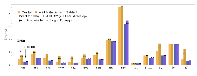
Refer to caption
Refer to caption
Figure 8: The effects of finite terms of top-loop diagrams on the Higgs coupling precision (upper panel) and operator constraints (lower) at the ILC 250 (yellow) and 500 stage (blue). For each case, two bars are shown: the first bar is just our full result that does not include the finite terms, while the second bar includes all the finite terms in Table 7. Also marked in the second bar is the result obtained with only finite terms proportional to ctBsubscript𝑐𝑡𝐵c_{tB} in δΓ(hγγ)𝛿Γ𝛾𝛾\delta\Gamma(h\to\gamma\gamma).

B.3 Higher-order effects of top quarks

channel 𝒪Htsubscript𝒪𝐻𝑡\mathcal{O}_{Ht} 𝒪Hq(1)superscriptsubscript𝒪𝐻𝑞1\mathcal{O}_{Hq}^{(1)} 𝒪Hq(3)superscriptsubscript𝒪𝐻𝑞3\mathcal{O}_{Hq}^{(3)} 𝒪Htbsubscript𝒪𝐻𝑡𝑏\mathcal{O}_{Htb} 𝒪tWsubscript𝒪𝑡𝑊\mathcal{O}_{tW} 𝒪tBsubscript𝒪𝑡𝐵\mathcal{O}_{tB} 𝒪tHsubscript𝒪𝑡𝐻\mathcal{O}_{tH}
hγγ𝛾𝛾h\to\gamma\gamma Our full 0 0 1.05 -0.03 28.07 51.24 -0.57
Without higher-order 0 0 0 0 28.02 51.05 -0.57
hZγ𝑍𝛾h\to Z\gamma Our full -0.71 0.14 2.26 -0.07 16.62 -2.79 -0.11
Without higher-order -0.29 -0.29 0.29 0 16.64 -2.93 -0.11
Table 8: The higher-order (two-loop) contributions of top quarks in the loop-induced Higgs decay widths. The coefficient of each top operator contribution is shown in absolute value with 1/v21superscript𝑣21/v^{2} normalization. Although two-loop originated, they are only one-loop suppressed compared to the SM contributions. The first line “Our full” shows the full results of this work including such higher-order effects while the second line without them. The higher-order effects were ignored in Durieux:2018ggn ; Vryonidou:2018eyv . The impact of higher-order effects is numerically explored in Fig. 9. Q=max(mt,Qproc)𝑄maxsubscript𝑚𝑡subscript𝑄procQ={\rm max}(m_{t},Q_{\rm proc}).

For δΓ(hγγ,Zγ)𝛿Γ𝛾𝛾𝑍𝛾\delta\Gamma(h\to\gamma\gamma,\,Z\gamma), Higgs operators contribute either through the tree-level renormalization of SM expressions (hence, cH,Tsubscript𝑐𝐻𝑇c_{H,T} at absolute one-loop) or through the tree-level contact interaction of hγγ𝛾𝛾h\gamma\gamma and hZγ𝑍𝛾hZ\gamma (hence, cWW,WB,BBsubscript𝑐𝑊𝑊𝑊𝐵𝐵𝐵c_{WW,WB,BB} at absolute tree-level). Since those widths are one-loop induced in the SM, our power counting insists on including absolute two-loop top-quark corrections. On the other hand, Ref. Durieux:2018ggn ; Vryonidou:2018eyv considered only absolute one-loop top corrections. To estimate their impact, the higher-order terms of top operators are extracted from our calculation and tabulated in Table 8.

Table 8 shows that largest higher-order effects come from cHt,Hq1,Hq3subscript𝑐𝐻𝑡𝐻𝑞1𝐻𝑞3c_{Ht,Hq1,Hq3} which renormalize cHsubscript𝑐𝐻c_{H} and cTsubscript𝑐𝑇c_{T}. Although these two-loop effects are smaller than the one-loop effects of ctW,tBsubscript𝑐𝑡𝑊𝑡𝐵c_{tW,tB} renormalizing the tree-level contact interactions induced by cWW,WB,BBsubscript𝑐𝑊𝑊𝑊𝐵𝐵𝐵c_{WW,WB,BB}131313Small higher-order effects proportional to ctW,tBsubscript𝑐𝑡𝑊𝑡𝐵c_{tW,tB} are from the renormalization of SM parameters such as δe𝛿𝑒\delta e and δmW𝛿subscript𝑚𝑊\delta m_{W}. As an aside, cHtbsubscript𝑐𝐻𝑡𝑏c_{Htb} terms are small proportional to ybsubscript𝑦𝑏y_{b}, and 𝒪tHsubscript𝒪𝑡𝐻{\cal O}_{tH} does not RG mix in our work., these 𝒪(0.11)𝒪0.11{\cal O}(0.1-1) terms are not small compared to most entries of top contributions in Table 11 (actually larger than most entries). This is consistent with an underlying logic of our power counting rule that the relative order matters. Moreover, higher-order effects can be leading contributions, e.g. for 𝒪Hq(3)superscriptsubscript𝒪𝐻𝑞3{\cal O}_{Hq}^{(3)} and 𝒪Htbsubscript𝒪𝐻𝑡𝑏{\cal O}_{Htb} in δΓ(hγγ,Zγ)𝛿Γ𝛾𝛾𝑍𝛾\delta\Gamma(h\to\gamma\gamma,\,Z\gamma).

Figure 9 shows the impact of higher-order terms by comparing the global-fit results with and without higher-order terms in Table 8. The results with higher-order terms are our full global-fit results. Compared to Fig. 8, higher-order effects are somewhat smaller in general (Higgs coupling precision in particular), partly because only two observables are modified by higher-order effects. But still, as stronger dataset becomes available, g(hZγ)𝑔𝑍𝛾g(hZ\gamma) precision and several operator constraints become sensitive to higher-order terms and change by 𝒪(1)𝒪1{\cal O}(1).

Refer to caption
Refer to caption
Figure 9: The effects of higher-order (two-loop) top contributions on the Higgs coupling precision (upper panel) and operator constraints (lower) at the ILC 250 (yellow) and 500 stage (blue). For each case, two bars are shown: the first bar is just our full result that includes the higher-order terms, while the second bar does not. Such top contributions are tabulated in Table 8.

Appendix C Results with different renormalization scale Q𝑄Q

Loop calculations necessarily involve the uncertainty due to the choice of the RG scale Q𝑄Q. We have chosen Q=max(mt,Qproc)𝑄maxsubscript𝑚𝑡subscript𝑄procQ={\rm max}(m_{t},Q_{\rm proc}) in the main text, but also introduced other choices Q=max(2mt,Qproc)𝑄max2subscript𝑚𝑡subscript𝑄procQ={\rm max}(2m_{t},Q_{\rm proc}) and Q=Qproc𝑄subscript𝑄procQ=Q_{\rm proc} in Section 3.5. In Fig. 10, we compare global-fit results with those three choices of Q𝑄Q.

First of all, the variations of the Higgs coupling precision and operator constraints are 𝒪(10%)similar-toabsent𝒪percent10\sim{\cal O}(10\%) at the ILC 250 with LHC Run 2. But stronger direct-top constraints from HL-LHC S2 make this variation from top effects smaller. One can expect that at the ILC 500, even though there will be more multiple scales, stronger direct-top data may not significantly increase the variation. These are the uncertainties in our results due to the choice of Q𝑄Q. In principle, this size of uncertainty is inevitable in perturbative calculations which can only be reduced by carrying out even higher-order calculations.

More interestingly, Higgs coupling precision is most robust against the addition of top-quark effects when Q=max(2mt,Qproc)𝑄max2subscript𝑚𝑡subscript𝑄procQ={\rm max}(2m_{t},Q_{\rm proc}) is used. This is already discussed in Section 5.2 as the main reason why Higgs coupling precision at the ILC can be robust against top effects; the more number of common scales in the fit observables, the better can Higgs couplings be semi-directly measured.

On the other hand, the very many common scales may harm operator constraints since top RG effects can only be discerned from multiple energy scales. Figure 10 indeed shows that operator constraints vary somewhat more than Higgs coupling precision. But notably, operator constraints also become most robust when Q=max(2mt,Qproc)𝑄max2subscript𝑚𝑡subscript𝑄procQ={\rm max}(2m_{t},Q_{\rm proc}), which provides more numbers of common energy scales 2mt2subscript𝑚𝑡2m_{t} so that RG effects are expected to be harder to discern. This is partly because 2mt2subscript𝑚𝑡2m_{t} is closer to Q0=1subscript𝑄01Q_{0}=1 TeV from which we RG evolve operators, so that RG effects with Q=max(2mt,Qproc)𝑄max2subscript𝑚𝑡subscript𝑄procQ={\rm max}(2m_{t},Q_{\rm proc}) are smaller than with other choices of Q𝑄Q.

Lastly, Fig. 11 (compared with Fig. 4) shows that the beam polarization becomes more important with Q=Qproc𝑄subscript𝑄procQ=Q_{\rm proc} than with other choices. As discussed in Section 5.3, it is because more various energy scales are involved so that the beam polarization can efficiently double the number of independent observables, disentangling the Higgs and top operators. Also, finite terms and higher-order effects may not be described by a small number of c~isubscript~𝑐𝑖\tilde{c}_{i} combinations (introduced in Section 5.2), which then make the beam polarization more useful.
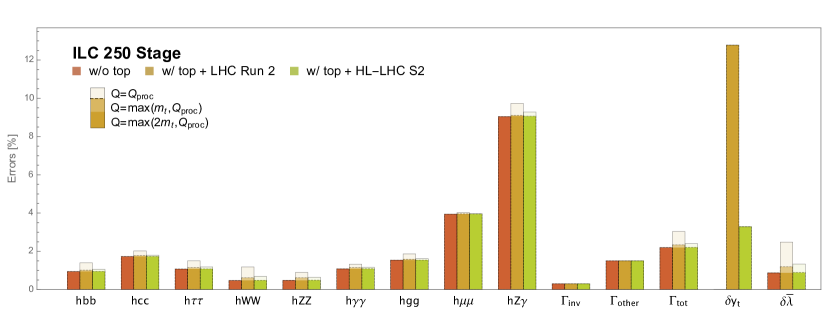
Refer to caption
Refer to caption
Figure 10: Global-fit results with various choice of Q=Qproc,max(mt,Qproc)𝑄subscript𝑄procmaxsubscript𝑚𝑡subscript𝑄procQ=Q_{\rm proc},\,{\rm max}(m_{t},Q_{\rm proc}) and max(2mt,Qproc)max2subscript𝑚𝑡subscript𝑄proc{\rm max}(2m_{t},Q_{\rm proc}) at the ILC 250 stage.
Refer to caption
Refer to caption
Figure 11: Same as Fig. 4 but with Q=Qproc𝑄subscript𝑄procQ=Q_{\rm proc}. Not only the variations due to top effects become larger, but also the impact of beam polarization becomes more visible.

Appendix D The Q0subscript𝑄0Q_{0} scale dependence

As introduced in Section 3.5, the Q0subscript𝑄0Q_{0} is a reference scale (different from the RG scale Q𝑄Q) at which we renormalize operators and express their constraints. This is arbitrary in the viewpoint of numerical analyses although this can be related to the new physics scale or the matching scale of the SMEFT. Numerically, our final results must not depend on the choice of Q0subscript𝑄0Q_{0}; unlike the case of Q𝑄Q, no inevitable numerical uncertainties are generated. This must imply one property of the covariance matrix: it should change with Q0subscript𝑄0Q_{0} in such a way to compensate the RG evolutions of Higgs operators. We detail this in Appendix D.1 and D.2, and apply this to understand the connection of cT(Q0)subscript𝑐𝑇subscript𝑄0c_{T}(Q_{0}) and oblique parameters in Appendix D.3.

D.1 The running of the covariance matrix

The measurements involved in our global fits are performed at various energy scales. Theory predictions are written in terms of the Wilson coefficients renormalized at Q0subscript𝑄0Q_{0}. The fit results then represent the constraints on the operator coefficients at Q0subscript𝑄0Q_{0}. If we change the Q0subscript𝑄0Q_{0} to Q0superscriptsubscript𝑄0Q_{0}^{\prime}, the constraints change as shown in Fig. 12.

As discussed in Section 5.1, the covariance matrix 𝒞ovIJ(Q0)𝒞𝑜subscript𝑣𝐼𝐽subscript𝑄0\mathcal{C}ov_{IJ}(Q_{0}) encodes the RG evolutions of operators from Q0subscript𝑄0Q_{0} to the RG scales of observables. It also changes with Q0subscript𝑄0Q_{0} in such a way to leave the total χ2superscript𝜒2\chi^{2} of the global fit unchanged

χ2=I,JcI(Q0)𝒞ovIJ1(Q0)cJ(Q0)=I,JcI(Q0)𝒞ovIJ1(Q0)cJ(Q0).superscript𝜒2subscript𝐼𝐽subscript𝑐𝐼subscript𝑄0𝒞𝑜subscriptsuperscript𝑣1𝐼𝐽subscript𝑄0subscript𝑐𝐽subscript𝑄0subscript𝐼𝐽subscript𝑐𝐼superscriptsubscript𝑄0𝒞𝑜subscriptsuperscript𝑣1𝐼𝐽superscriptsubscript𝑄0subscript𝑐𝐽superscriptsubscript𝑄0\chi^{2}=\sum_{I,J}c_{I}(Q_{0})\,\mathcal{C}ov^{-1}_{IJ}(Q_{0})\,c_{J}(Q_{0})=\sum_{I,J}c_{I}(Q_{0}^{\prime})\,\mathcal{C}ov^{-1}_{IJ}(Q_{0}^{\prime})\,c_{J}(Q_{0}^{\prime}). (42)

The Wilson coefficients cI(Q0)subscript𝑐𝐼subscript𝑄0c_{I}(Q_{0}) RG evolve as

cI(Q0)=(ci(Q0)cj(Q0))=(1iiγijlog(Q0/Q0)01jj)(ci(Q0)cj(Q0))ΓIJ(Q0/Q0)cJ(Q0),subscript𝑐𝐼superscriptsubscript𝑄0subscript𝑐𝑖superscriptsubscript𝑄0subscript𝑐𝑗superscriptsubscript𝑄0subscript1𝑖superscript𝑖subscript𝛾𝑖superscript𝑗superscriptsubscript𝑄0subscript𝑄00subscript1𝑗superscript𝑗subscript𝑐superscript𝑖subscript𝑄0subscript𝑐superscript𝑗subscript𝑄0subscriptΓ𝐼𝐽superscriptsubscript𝑄0subscript𝑄0subscript𝑐𝐽subscript𝑄0c_{I}(Q_{0}^{\prime})=\left({\begin{array}[]{c}c_{i}(Q_{0}^{\prime})\\ c_{j}(Q_{0}^{\prime})\end{array}}\right)\,=\,\left({\begin{array}[]{cc}1_{ii^{\prime}}&\gamma_{ij^{\prime}}\log(Q_{0}^{\prime}/Q_{0})\\ 0&1_{jj^{\prime}}\end{array}}\right)\left({\begin{array}[]{c}c_{i^{\prime}}(Q_{0})\\ c_{j^{\prime}}(Q_{0})\end{array}}\right)\,\equiv\,\Gamma_{IJ}(Q_{0}^{\prime}/Q_{0})\,c_{J}(Q_{0}), (43)

where the upper(lower) components ci(cj)subscript𝑐𝑖subscript𝑐𝑗c_{i}(c_{j}) denote the coefficients of Higgs(top) operators and I,J𝐼𝐽I,J denote the indices i,j𝑖𝑗i,j collectively. The block diagonal form of ΓIJsubscriptΓ𝐼𝐽\Gamma_{IJ} is from our scheme where only the RG evolutions of Higgs operators by top operators are considered. Thus, the covariance matrix must evolve as

𝒞ov(Q0)=Γ(Q0/Q0)𝒞ov(Q0)Γ(Q0/Q0)T.𝒞𝑜𝑣superscriptsubscript𝑄0Γsuperscriptsubscript𝑄0subscript𝑄0𝒞𝑜𝑣subscript𝑄0Γsuperscriptsuperscriptsubscript𝑄0subscript𝑄0𝑇\mathcal{C}ov(Q_{0}^{\prime})=\Gamma(Q_{0}^{\prime}/Q_{0})~{}\mathcal{C}ov(Q_{0})~{}\Gamma(Q_{0}^{\prime}/Q_{0})^{T}. (44)

Again, this evolution ensures that global-fit results obtained with different Q0subscript𝑄0Q_{0} are physically equivalent (same χ2superscript𝜒2\chi^{2}), and one result can be obtained from the other through the evolution of the covariance matrix.

As an aside, we mention properties of the evolution of covariance matrix. Note that Γ1(Q/Q)=Γ(Q/Q)superscriptΓ1𝑄superscript𝑄Γsuperscript𝑄𝑄\Gamma^{-1}(Q/Q^{\prime})=\Gamma(Q^{\prime}/Q) and Γ(Q′′/Q)Γ(Q/Q)=Γ(Q′′/Q)Γsuperscript𝑄′′superscript𝑄Γsuperscript𝑄𝑄Γsuperscript𝑄′′𝑄\Gamma(Q^{\prime\prime}/Q^{\prime})\Gamma(Q^{\prime}/Q)=\Gamma(Q^{\prime\prime}/Q) make the evolution similar to (RG-)logarithmic. The diagonal component of the covariance matrix 𝒞ovII𝒞𝑜subscript𝑣𝐼𝐼\mathcal{C}ov_{II} is an error of a corresponding Wilson coefficient, and the off-diagonal element 𝒞ovIJ𝒞𝑜subscript𝑣𝐼𝐽\mathcal{C}ov_{IJ} is the error correlation between cIsubscript𝑐𝐼c_{I} and cJsubscript𝑐𝐽c_{J}. These components evolve as

𝒞ovII(Q0)=𝒞ovII(Q0)+J2γIJlog(Q0/Q0)𝒞ovIJ(Q0)𝒞𝑜subscript𝑣𝐼𝐼superscriptsubscript𝑄0𝒞𝑜subscript𝑣𝐼𝐼subscript𝑄0subscript𝐽2subscript𝛾𝐼𝐽superscriptsubscript𝑄0subscript𝑄0𝒞𝑜subscript𝑣𝐼𝐽subscript𝑄0\displaystyle\mathcal{C}ov_{II}(Q_{0}^{\prime})=\mathcal{C}ov_{II}(Q_{0})+\sum_{J}2\gamma_{IJ}\log(Q_{0}^{\prime}/Q_{0})\mathcal{C}ov_{IJ}(Q_{0}) (45)
+J(γIJlog(Q0/Q0))2𝒞ovJJ(Q0).subscript𝐽superscriptsubscript𝛾𝐼𝐽superscriptsubscript𝑄0subscript𝑄02𝒞𝑜subscript𝑣𝐽𝐽subscript𝑄0\displaystyle+\sum_{J}(\gamma_{IJ}\log(Q_{0}^{\prime}/Q_{0}))^{2}\mathcal{C}ov_{JJ}(Q_{0}).

For coefficients that do not RG evolve by top operators, the equation reduces to 𝒞ovII(Q0)=𝒞ovII(Q0)𝒞𝑜subscript𝑣𝐼𝐼subscript𝑄0𝒞𝑜subscript𝑣𝐼𝐼superscriptsubscript𝑄0\mathcal{C}ov_{II}(Q_{0})=\mathcal{C}ov_{II}(Q_{0}^{\prime}). Thus their constraints do not change with Q0subscript𝑄0Q_{0}. Examples include the constraints on top operators and c3Wsubscript𝑐3𝑊c_{3W} as shown in Fig. 12.

Refer to caption
Figure 12: The comparison of global fits performed with Q0=mhsubscript𝑄0subscript𝑚Q_{0}=m_{h} and 1 TeV. The two result are equivalent because one of them can be obtained by the other via the RG evolution of the covariance matrix. It also shows that 𝒪Tsubscript𝒪𝑇{\cal O}_{T} runs most quickly due to top operators.

D.2 The Q0subscript𝑄0Q_{0} independence of the uncertainty of observables

The evolution of the covariance matrix also ensures that the (physical) results defined at certain Qprocsubscript𝑄procQ_{\rm proc} (such as Higgs coupling precision and oblique parameters) are independent on Q0subscript𝑄0Q_{0}. Start from the theory prediction of the deviations of the observable δ𝒪𝛿𝒪\delta{\cal O} defined at Q𝑄Q

δ𝒪(Q)=IaI(Q)cI(Q)=I,JaI(Q)ΓIJ(Q/Q0)cJ(Q0)=JaJ(Q0)cJ(Q0),𝛿𝒪𝑄subscript𝐼subscript𝑎𝐼𝑄subscript𝑐𝐼𝑄subscript𝐼𝐽subscript𝑎𝐼𝑄subscriptΓ𝐼𝐽𝑄subscript𝑄0subscript𝑐𝐽subscript𝑄0subscript𝐽subscript𝑎𝐽subscript𝑄0subscript𝑐𝐽subscript𝑄0\delta\mathcal{O}(Q)=\sum_{I}a_{I}(Q)\,c_{I}(Q)=\sum_{I,J}a_{I}(Q)\Gamma_{IJ}(Q/Q_{0})\,c_{J}(Q_{0})=\sum_{J}a_{J}(Q_{0})\,c_{J}(Q_{0}), (46)

where aIsubscript𝑎𝐼a_{I} is the constant multiplied in front of each Wilson coefficient cIsubscript𝑐𝐼c_{I}, i.e. numbers collected in Table 10 and 11. This determines the rule for the transformation of aIsubscript𝑎𝐼a_{I} with the energy scale. Given the covariance matrix from a global fit, one can calculate the error of the observable 𝒪𝒪\mathcal{O} contributed from EFT operators as

σ𝒪2=δ𝒪2superscriptsubscript𝜎𝒪2delimited-⟨⟩𝛿superscript𝒪2\displaystyle\sigma_{\mathcal{O}}^{2}=\left<\delta\mathcal{O}^{2}\right> =\displaystyle= I,JaI(Q)𝒞ovIJ(Q)aJ(Q)subscript𝐼𝐽subscript𝑎𝐼𝑄𝒞𝑜subscript𝑣𝐼𝐽𝑄subscript𝑎𝐽𝑄\displaystyle\sum_{I,J}a_{I}(Q)\mathcal{C}ov_{IJ}(Q)a_{J}(Q)
=\displaystyle= I,J,K,LaI(Q)ΓIK(Q/Q0)𝒞ovKL(Q0)ΓJL(Q/Q0)aJ(Q)subscript𝐼𝐽𝐾𝐿subscript𝑎𝐼𝑄subscriptΓ𝐼𝐾𝑄subscript𝑄0𝒞𝑜subscript𝑣𝐾𝐿subscript𝑄0subscriptΓ𝐽𝐿𝑄subscript𝑄0subscript𝑎𝐽𝑄\displaystyle\sum_{I,J,K,L}a_{I}(Q)\Gamma_{IK}(Q/Q_{0})\,\mathcal{C}ov_{KL}(Q_{0})\,\Gamma_{JL}(Q/Q_{0})a_{J}(Q)
=\displaystyle= I,JaI(Q0)𝒞ovIJ(Q0)aJ(Q0).subscript𝐼𝐽subscript𝑎𝐼subscript𝑄0𝒞𝑜subscript𝑣𝐼𝐽subscript𝑄0subscript𝑎𝐽subscript𝑄0\displaystyle\sum_{I,J}a_{I}(Q_{0})\mathcal{C}ov_{IJ}(Q_{0})a_{J}(Q_{0}).

The second line follows from the matrix relation in Eq. (44). This proves that the error of a physical observable contributed from EFT coefficients is independent on our choice of Q0subscript𝑄0Q_{0}.

D.3 The interpretation of the Q0subscript𝑄0Q_{0} dependence - Oblique parameters

We turn to discuss one interesting Q0subscript𝑄0Q_{0} dependence, which provides another example of how to think of Q0subscript𝑄0Q_{0}. Figure 12 shows that the constraint on cTsubscript𝑐𝑇c_{T} varies significantly with Q0subscript𝑄0Q_{0}, because cTsubscript𝑐𝑇c_{T} receives a large anomalous dimension from top operators. As a result, its constraint is much weaker at higher Q0subscript𝑄0Q_{0} scales. Since cTsubscript𝑐𝑇c_{T} is closely related to the T𝑇T parameter that signals the breaking of the custodial symmetry, does this mean that the custodial symmetry can be broken seriously at high energy? Not necessarily.

αS𝛼𝑆\alpha S αT𝛼𝑇\alpha T
 ILC 250+500 without top operators  0.0189 %  0.0175 %
 With top operators (indirect-only)  0.0268 %  0.0177 %
 + HL-LHC S2  0.0201 %  0.0175 %
 + ILC 500 direct-top  0.0189 %  0.0175 %
Table 9: Global-fit constraints on the oblique parameters, αS𝛼𝑆\alpha\,S and αT𝛼𝑇\alpha\,T in Eq. (49). They are defined at Qproc=mZsubscript𝑄procsubscript𝑚𝑍Q_{\rm proc}=m_{Z}, hence top-quark effects are evaluated at Q=max(mt,mZ)=mt𝑄maxsubscript𝑚𝑡subscript𝑚𝑍subscript𝑚𝑡Q={\rm max}(m_{t},m_{Z})=m_{t}. Any choice of Q0subscript𝑄0Q_{0} yields the same results.

We detail these by explicitly checking that our global fit successfully impose the small breaking of the custodial symmetry at low energy mZsimilar-toabsentsubscript𝑚𝑍\sim m_{Z} (irrespective of Q0subscript𝑄0Q_{0}) even though we do not directly use small T𝑇T as an input data. The expressions of oblique parameters can be read from the expressions of well-measured electroweak precision observables, Z𝑍Z-pole ssubscript𝑠s_{*} and mW2/mZ2superscriptsubscript𝑚𝑊2superscriptsubscript𝑚𝑍2m_{W}^{2}/m_{Z}^{2}Barklow:2017awn

mW2/mZ2superscriptsubscript𝑚𝑊2superscriptsubscript𝑚𝑍2\displaystyle m_{W}^{2}/m_{Z}^{2} =\displaystyle= c02+c02c02s02(c02cT2s02(cHL+8cWB)),superscriptsubscript𝑐02superscriptsubscript𝑐02superscriptsubscript𝑐02superscriptsubscript𝑠02superscriptsubscript𝑐02subscript𝑐𝑇2superscriptsubscript𝑠02superscriptsubscript𝑐𝐻𝐿8subscript𝑐𝑊𝐵\displaystyle c_{0}^{2}\,+\,\frac{c_{0}^{2}}{c_{0}^{2}-s_{0}^{2}}\left(c_{0}^{2}\,c_{T}-2s_{0}^{2}(c_{HL}^{\prime}+8c_{WB})\right),
s2superscriptsubscript𝑠2\displaystyle s_{*}^{2} =\displaystyle= s02+s02c02s02(cHL+8cWBc02cT)12cHEs02(cHLcHE),superscriptsubscript𝑠02superscriptsubscript𝑠02superscriptsubscript𝑐02superscriptsubscript𝑠02superscriptsubscript𝑐𝐻𝐿8subscript𝑐𝑊𝐵superscriptsubscript𝑐02subscript𝑐𝑇12subscript𝑐𝐻𝐸superscriptsubscript𝑠02subscript𝑐𝐻𝐿subscript𝑐𝐻𝐸\displaystyle s_{0}^{2}\,+\,\frac{s_{0}^{2}}{c_{0}^{2}-s_{0}^{2}}\left(c_{HL}^{\prime}+8c_{WB}-c_{0}^{2}c_{T}\right)\,-\,\frac{1}{2}c_{HE}\,-\,s_{0}^{2}(c_{HL}-c_{HE}), (48)

as (generalized from Barklow:2017awn )

αS𝛼𝑆\displaystyle\alpha\,S =\displaystyle= 4s02(8cWB+cHL)+ 4(12+s02)cHE 4s02cHL,4superscriptsubscript𝑠028subscript𝑐𝑊𝐵superscriptsubscript𝑐𝐻𝐿412superscriptsubscript𝑠02subscript𝑐𝐻𝐸4superscriptsubscript𝑠02subscript𝑐𝐻𝐿\displaystyle 4s_{0}^{2}\,(8c_{WB}+c_{HL}^{\prime})\,+\,4\left(-\frac{1}{2}+s_{0}^{2}\right)c_{HE}\,-\,4s_{0}^{2}c_{HL},
αT𝛼𝑇\displaystyle\alpha\,T =\displaystyle= cTc02s02c02cHE 2s02c02cHL.subscript𝑐𝑇superscriptsubscript𝑐02superscriptsubscript𝑠02superscriptsubscript𝑐02subscript𝑐𝐻𝐸2superscriptsubscript𝑠02superscriptsubscript𝑐02subscript𝑐𝐻𝐿\displaystyle c_{T}\,-\,\frac{c_{0}^{2}-s_{0}^{2}}{c_{0}^{2}}c_{HE}\,-\,2\frac{s_{0}^{2}}{c_{0}^{2}}c_{HL}. (49)

These are Z𝑍Z-pole observables, hence defined at Qproc=mZsubscript𝑄procsubscript𝑚𝑍Q_{\rm proc}=m_{Z}. The expressions are consistent with the oblique parameters, S^^𝑆\hat{S} and T^^𝑇\hat{T}, defined in the universal limit Wells:2015uba

S^^𝑆\displaystyle\hat{S} \displaystyle\equiv α4s02S=g2(1ggCHWB+14CHJW+14CHJB),𝛼4superscriptsubscript𝑠02𝑆superscript𝑔21𝑔superscript𝑔subscript𝐶𝐻𝑊𝐵14subscript𝐶𝐻𝐽𝑊14subscript𝐶𝐻𝐽𝐵\displaystyle\frac{\alpha}{4s_{0}^{2}}S\,=\,g^{2}(\frac{1}{gg^{\prime}}C_{HWB}\,+\,\frac{1}{4}C_{HJW}\,+\,\frac{1}{4}C_{HJB}), (50)
T^^𝑇\displaystyle\hat{T} \displaystyle\equiv αT=12CHD+g 22CHJB,𝛼𝑇12subscript𝐶𝐻𝐷superscript𝑔22subscript𝐶𝐻𝐽𝐵\displaystyle\alpha T\,=\,-\frac{1}{2}C_{HD}\,+\,\frac{g^{\prime\,2}}{2}C_{HJB}, (51)

because our operators correspond to the bosonic currents in the universal theory

cHLg24CHJW,cHLg 22YlCHJB,cHEg 22YeCHJB,formulae-sequencesuperscriptsubscript𝑐𝐻𝐿superscript𝑔24subscript𝐶𝐻𝐽𝑊formulae-sequencesubscript𝑐𝐻𝐿superscript𝑔22subscript𝑌𝑙subscript𝐶𝐻𝐽𝐵subscript𝑐𝐻𝐸superscript𝑔22subscript𝑌𝑒subscript𝐶𝐻𝐽𝐵c_{HL}^{\prime}\,\to\,\frac{g^{2}}{4}C_{HJW},\quad c_{HL}\,\to\,\frac{g^{\prime\,2}}{2}Y_{l}\,C_{HJB},\quad c_{HE}\,\to\,\frac{g^{\prime\,2}}{2}Y_{e}\,C_{HJB}, (52)

where Yl,esubscript𝑌𝑙𝑒Y_{l,\,e} are the hypercharges of the L𝐿L and e𝑒e, respectively.

Using these, we numerically evaluate the global-fit constraints on αS𝛼𝑆\alpha S and αT𝛼𝑇\alpha T in Table 9. Whether top operators are added or not, they are indeed constrained to be small for all benchmark scenarios. Top-quark effects on oblique parameters are particularly small once direct-top constraints are included. The oblique parameters are defined at Qproc=mZsubscript𝑄procsubscript𝑚𝑍Q_{\rm proc}=m_{Z}, while top-quark effects are decoupled below mtsubscript𝑚𝑡m_{t} so that Q=max(mt,mZ)=mt𝑄maxsubscript𝑚𝑡subscript𝑚𝑍subscript𝑚𝑡Q={\rm max}(m_{t},m_{Z})=m_{t} is used. Thus, (we checked that) these results remain true and same for any value of Q0subscript𝑄0Q_{0}, again because the constraints on physical observables are independent on Q0subscript𝑄0Q_{0}. The Q0subscript𝑄0Q_{0}-independence implies that the custodial symmetry is well preserved at low energy regardless of cTsubscript𝑐𝑇c_{T} constraints at high Q0subscript𝑄0Q_{0}.

What about the custodial symmetry at high energy scales (where cTsubscript𝑐𝑇c_{T} is weakly constrained)? First of all, cTsubscript𝑐𝑇c_{T} (at high Q0subscript𝑄0Q_{0}) does not necessarily correspond to the T𝑇T parameter. Eq. (49) shows that there can be other contributions to EW precision observables because our operator set is not assumed to be oblique or universal. At high energy scales, the meaning of T𝑇T becomes more subtle too. One main reason is that the S,T,U𝑆𝑇𝑈S,T,U description is valid at low energy, as this is the Taylor expansion of self-energy corrections in powers of energy scale Peskin:1990zt . Also, the RG evolution itself generates the non-universal effects which cannot be absorbed into the parameters of universal theories Wells:2015cre . It is expected that the non-universal effects interfere with the universal ones, making the meaning of T𝑇T ambiguous. Therefore, the poor constraint on cTsubscript𝑐𝑇c_{T} at high Q0subscript𝑄0Q_{0} does not necessarily mean the large breaking of the custodial symmetry at those high scales, nor at low scales.

Appendix E RG evolution with bottom operators and their impact

Our main discussion focuses on the Higgs and top operators. But many new physics models accompany bottom operators together with top operators. The following 3 ‘bottom’ operators are relevant to us (in addition to the bottom Yukawa operator 𝒪bHsubscript𝒪𝑏𝐻{\cal O}_{bH} that is already added)

𝒪Hbsubscript𝒪𝐻𝑏\displaystyle\mathcal{O}_{Hb} =\displaystyle= (ΦiDμΦ)(b¯γμb),superscriptΦ𝑖subscript𝐷𝜇Φ¯𝑏superscript𝛾𝜇𝑏\displaystyle(\Phi^{\dagger}i\overleftrightarrow{D}_{\mu}\Phi)(\bar{b}\gamma^{\mu}b),
𝒪bWsubscript𝒪𝑏𝑊\displaystyle\mathcal{O}_{bW} =\displaystyle= (Q¯τaσμνb)ΦWμνa,¯𝑄superscript𝜏𝑎superscript𝜎𝜇𝜈𝑏Φsuperscriptsubscript𝑊𝜇𝜈𝑎\displaystyle(\bar{Q}\tau^{a}\sigma^{\mu\nu}b)\Phi W_{\mu\nu}^{a}, (53)
𝒪bBsubscript𝒪𝑏𝐵\displaystyle\mathcal{O}_{bB} =\displaystyle= (Q¯σμνb)ΦBμν,¯𝑄superscript𝜎𝜇𝜈𝑏Φsubscript𝐵𝜇𝜈\displaystyle(\bar{Q}\sigma^{\mu\nu}b)\Phi B_{\mu\nu},

with the Lagrangian

Δbottom=cHbv2𝒪Hb+cbWv2𝒪bW+cbBv2𝒪bB.Δsubscriptbottomsubscript𝑐𝐻𝑏superscript𝑣2subscript𝒪𝐻𝑏subscript𝑐𝑏𝑊superscript𝑣2subscript𝒪𝑏𝑊subscript𝑐𝑏𝐵superscript𝑣2subscript𝒪𝑏𝐵\Delta{\cal L}_{\rm bottom}\,=\,\frac{c_{Hb}}{v^{2}}\,\mathcal{O}_{Hb}\,+\,\frac{c_{bW}}{v^{2}}\,\mathcal{O}_{bW}\,+\,\frac{c_{bB}}{v^{2}}\,\mathcal{O}_{bB}. (54)

These operators are relevant in direct-top and -bottom observables at tree-level as well as Higgs + EW observables at one-loop. The tree-level effects on direct-top constraints are already taken into account in Durieux:2019rbz , from which we take our direct-top constraints.

The RG equations of dimension-6 operators are given in Alonso:2013hga ; Grojean:2013kd ; Jenkins:2013zja ; Jenkins:2013wua . Their Warsaw-basis operators can be converted to ours following the rule

cH=2cH+12cHD,subscript𝑐𝐻2subscript𝑐𝐻12subscript𝑐𝐻𝐷\displaystyle c_{H}=-2c_{H\square}+\frac{1}{2}c_{HD},~{} cT=12cHD,subscript𝑐𝑇12subscript𝑐𝐻𝐷\displaystyle~{}c_{T}=-\frac{1}{2}c_{HD},~{} λv2c6=1v2cHH,𝜆superscript𝑣2subscript𝑐61superscript𝑣2subscript𝑐𝐻𝐻\displaystyle~{}-\frac{\lambda}{v^{2}}c_{6}=\frac{1}{v^{2}}c_{HH},
g2mW2cWW=1v2cHW,superscript𝑔2superscriptsubscript𝑚𝑊2subscript𝑐𝑊𝑊1superscript𝑣2subscript𝑐𝐻𝑊\displaystyle\frac{g^{2}}{m_{W}^{2}}c_{WW}=\frac{1}{v^{2}}c_{HW},~{} g2mW2cBB=1v2cHB,superscript𝑔2superscriptsubscript𝑚𝑊2subscript𝑐𝐵𝐵1superscript𝑣2subscript𝑐𝐻𝐵\displaystyle~{}\frac{g^{\prime 2}}{m_{W}^{2}}c_{BB}=\frac{1}{v^{2}}c_{HB},~{} 2ggmW2cWB=1v2cHWB,2𝑔superscript𝑔superscriptsubscript𝑚𝑊2subscript𝑐𝑊𝐵1superscript𝑣2subscript𝑐𝐻𝑊𝐵\displaystyle~{}\frac{2gg^{\prime}}{m_{W}^{2}}c_{WB}=\frac{1}{v^{2}}c_{HWB},
1v2cHL=1v2cHl(1),1superscript𝑣2subscript𝑐𝐻𝐿1superscript𝑣2superscriptsubscript𝑐𝐻𝑙1\displaystyle\frac{1}{v^{2}}c_{HL}=\frac{1}{v^{2}}c_{Hl}^{(1)},~{} 1v2cHL=1v2cHl(3),1superscript𝑣2superscriptsubscript𝑐𝐻𝐿1superscript𝑣2superscriptsubscript𝑐𝐻𝑙3\displaystyle~{}\frac{1}{v^{2}}c_{HL}^{\prime}=\frac{1}{v^{2}}c_{Hl}^{(3)},~{} 1v2cHE=1v2cHe,1superscript𝑣2subscript𝑐𝐻𝐸1superscript𝑣2subscript𝑐𝐻𝑒\displaystyle~{}\frac{1}{v^{2}}c_{HE}=\frac{1}{v^{2}}c_{He}, (55)

where operators on the right-hand side are the operators in Alonso:2013hga and on the left-hand side are ours; to avoid confusion, we use cHHsubscript𝑐𝐻𝐻c_{HH} instead of cHsubscript𝑐𝐻c_{H} on the right-hand side. We keep only top contributions to Higgs operators. Keeping terms of order 𝒪(g,g,yt,yb)2𝒪superscript𝑔superscript𝑔subscript𝑦𝑡subscript𝑦𝑏2{\cal O}(g,\,g^{\prime},\,y_{t},\,y_{b})^{2}, we already showed all the needed top-operator contributions in Section 3.5. In addition, for completeness, we show the RG equations of c6subscript𝑐6c_{6} and cbHsubscript𝑐𝑏𝐻c_{bH} as well as additional bottom contributions to Higgs operators

c˙6subscript˙𝑐6\displaystyle\dot{c}_{6} =\displaystyle= 1λ[(8λytNc8yt3Nc)ctH+(16λyt2Nc+163λg2)cHq(3)+16λytybNccHtb],1𝜆delimited-[]8𝜆subscript𝑦𝑡subscript𝑁𝑐8superscriptsubscript𝑦𝑡3subscript𝑁𝑐subscript𝑐𝑡𝐻16𝜆superscriptsubscript𝑦𝑡2subscript𝑁𝑐163𝜆superscript𝑔2superscriptsubscript𝑐𝐻𝑞316𝜆subscript𝑦𝑡subscript𝑦𝑏subscript𝑁𝑐subscript𝑐𝐻𝑡𝑏\displaystyle-\frac{1}{\lambda}\left[(8\lambda y_{t}N_{c}-8y_{t}^{3}N_{c})c_{tH}+(-16\lambda y_{t}^{2}N_{c}+\frac{16}{3}\lambda g^{2})c_{Hq}^{(3)}+16\lambda y_{t}y_{b}N_{c}c_{Htb}\right], (56)
c˙bHsubscript˙𝑐𝑏𝐻\displaystyle\dot{c}_{bH} =\displaystyle= yt(2Nc3)ctH+((4Nc+6)yt22g12+43g22Nc+12λ)cHq(3)subscript𝑦𝑡2subscript𝑁𝑐3subscript𝑐𝑡𝐻4subscript𝑁𝑐6superscriptsubscript𝑦𝑡22superscriptsubscript𝑔1243superscriptsubscript𝑔22subscript𝑁𝑐12𝜆superscriptsubscript𝑐𝐻𝑞3\displaystyle y_{t}(2N_{c}-3)c_{tH}\,+\,\left((-4N_{c}+6)y_{t}^{2}-2g_{1}^{2}+\tfrac{4}{3}g_{2}^{2}N_{c}+12\lambda\right)c_{Hq}^{(3)} (57)
+(2g12+4λ)cHq(1)+(2yt3+3g22yt4λyt)/ybcHtb+(6g2yt)ctW.2superscriptsubscript𝑔124𝜆superscriptsubscript𝑐𝐻𝑞12superscriptsubscript𝑦𝑡33superscriptsubscript𝑔22subscript𝑦𝑡4𝜆subscript𝑦𝑡subscript𝑦𝑏subscript𝑐𝐻𝑡𝑏6subscript𝑔2subscript𝑦𝑡subscript𝑐𝑡𝑊\displaystyle\,+\,(-2g_{1}^{2}+4\lambda)c_{Hq}^{(1)}\,+\,(-2y_{t}^{3}+3g_{2}^{2}y_{t}-4\lambda y_{t})/y_{b}c_{Htb}\,+\,(-6g_{2}y_{t})c_{tW}.

The RG effect on cbHsubscript𝑐𝑏𝐻c_{bH} does not vanish in the limit yb0subscript𝑦𝑏0y_{b}\to 0 but is rather enhanced by yt/ybsubscript𝑦𝑡subscript𝑦𝑏y_{t}/y_{b}.

The bottom-operator RG contributions are (in addition to the top contributions in Section 3.5)

c˙Hsubscript˙𝑐𝐻\displaystyle\dot{c}_{H} =\displaystyle= 0,0\displaystyle 0, (58)
c˙Tsubscript˙𝑐𝑇\displaystyle\dot{c}_{T} =\displaystyle= (4Ncyb2+83g2YhYdNc)cHb,4subscript𝑁𝑐superscriptsubscript𝑦𝑏283superscript𝑔2subscript𝑌subscript𝑌𝑑subscript𝑁𝑐subscript𝑐𝐻𝑏\displaystyle-(4N_{c}y_{b}^{2}\,+\,\frac{8}{3}g^{\prime 2}Y_{h}Y_{d}N_{c})\,c_{Hb}, (59)
c˙WWsubscript˙𝑐𝑊𝑊\displaystyle\dot{c}_{WW} =\displaystyle= 12gNc(ybcbW),12𝑔subscript𝑁𝑐subscript𝑦𝑏subscript𝑐𝑏𝑊\displaystyle-\frac{1}{2}gN_{c}\,(y_{b}\,c_{bW}), (60)
c˙BBsubscript˙𝑐𝐵𝐵\displaystyle\dot{c}_{BB} =\displaystyle= 1tW2gNc(yb(Yq+Yd)cbB),1superscriptsubscript𝑡𝑊2superscript𝑔subscript𝑁𝑐subscript𝑦𝑏subscript𝑌𝑞subscript𝑌𝑑subscript𝑐𝑏𝐵\displaystyle-\frac{1}{t_{W}^{2}}g^{\prime}N_{c}(y_{b}(Y_{q}\,+\,Y_{d})\,c_{bB}), (61)
c˙WBsubscript˙𝑐𝑊𝐵\displaystyle\dot{c}_{WB} =\displaystyle= 18tW(2gNcybcbB 4g(Yq+Yd)ybNccbW),18subscript𝑡𝑊2𝑔subscript𝑁𝑐subscript𝑦𝑏subscript𝑐𝑏𝐵4superscript𝑔subscript𝑌𝑞subscript𝑌𝑑subscript𝑦𝑏subscript𝑁𝑐subscript𝑐𝑏𝑊\displaystyle\frac{1}{8t_{W}}(-2gN_{c}y_{b}\,c_{bB}\,-\,4g^{\prime}(Y_{q}\,+\,Y_{d})y_{b}N_{c}\,c_{bW}), (62)
c˙HLsubscript˙𝑐𝐻𝐿\displaystyle\dot{c}_{HL} =\displaystyle= 12Ylg2(83YdNccHb),12subscript𝑌𝑙superscript𝑔283subscript𝑌𝑑subscript𝑁𝑐subscript𝑐𝐻𝑏\displaystyle\frac{1}{2}Y_{l}g^{\prime 2}(\frac{8}{3}Y_{d}N_{c}\,c_{Hb}), (63)
c˙HLsuperscriptsubscript˙𝑐𝐻𝐿\displaystyle\dot{c}_{HL}^{\prime} =\displaystyle= 0,0\displaystyle 0, (64)
c˙HEsubscript˙𝑐𝐻𝐸\displaystyle\dot{c}_{HE} =\displaystyle= 12Yeg2(83YdNccHb).12subscript𝑌𝑒superscript𝑔283subscript𝑌𝑑subscript𝑁𝑐subscript𝑐𝐻𝑏\displaystyle\frac{1}{2}Y_{e}g^{\prime 2}(\frac{8}{3}Y_{d}N_{c}\,c_{Hb}). (65)

Figure 13 compares the global-fit results with and without the bottom operators. The bottom operators are well constrained by HL-LHC data, which include direct-bottom productions from Zbb¯𝑍𝑏¯𝑏Z\to b\bar{b} and single-top productions Durieux:2019rbz . Their RG effects are also often suppressed by small ybsubscript𝑦𝑏y_{b}. After all, the impact of bottom operators are almost invisible. We can safely ignore bottom operators assuming that direct-top and bottom data can constrain them well.
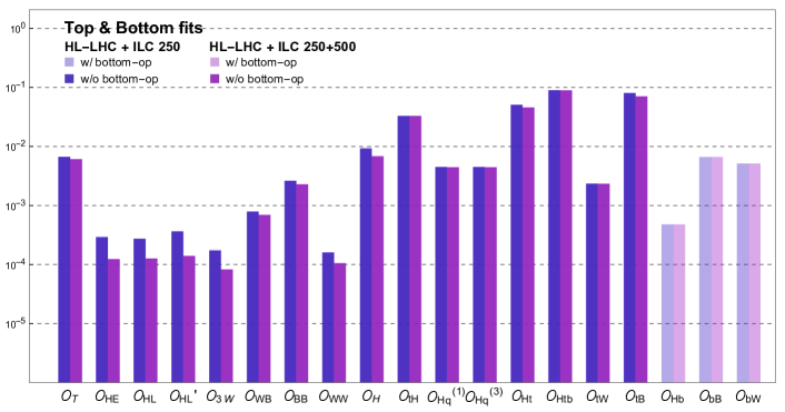
Refer to caption
Figure 13: The global-fit 1σ1𝜎1\sigma constraints with (dark) and without (light) the bottom operators in Eq. (E) added to our work. The changes due to bottom operators are almost invisible.

Appendix F Observables in terms of operators

Higgs Operators Observables cTsubscript𝑐𝑇c_{T} cHEsubscript𝑐𝐻𝐸c_{HE} cHLsubscript𝑐𝐻𝐿c_{HL} cHLsuperscriptsubscript𝑐𝐻𝐿c_{HL}^{\prime} c3Wsubscript𝑐3𝑊c_{3W} cWBsubscript𝑐𝑊𝐵c_{WB} cBBsubscript𝑐𝐵𝐵c_{BB} cWWsubscript𝑐𝑊𝑊c_{WW} cHsubscript𝑐𝐻c_{H} δα1𝛿superscript𝛼1\delta\alpha^{-1} 0 0 0 0 0 3.704 -1.852 -1.852 0 δGF𝛿subscript𝐺𝐹\delta G_{F} 0 0 0 2.0 0 0 0 0 0 δAl𝛿subscript𝐴𝑙\delta A_{l} 0 14.37 12.39 12.39 0 -53.23 -22.95 76.18 0 δmW𝛿subscript𝑚𝑊\delta m_{W} 0 0 0 0 0 0 0 4.0 0 δmZ𝛿subscript𝑚𝑍\delta m_{Z} -0.5 0 0 0 0 1.852 0.279 3.074 0 δmh𝛿subscript𝑚\delta m_{h} 0 0 0 0 0 0 0 0 -0.5 δΓl𝛿subscriptΓ𝑙\delta\Gamma_{l} -0.5 -1.84 2.14 2.14 0 4.97 0.58 10.06 0 δΓW𝛿subscriptΓ𝑊\delta\Gamma_{W} 0 0 0 0 0 0 0 12 0 δΓZ𝛿subscriptΓ𝑍\delta\Gamma_{Z} -0.5 0 0 0 0 5.03 0.61 9.97 0 δgZeff𝛿subscript𝑔𝑍𝑒𝑓𝑓\delta g_{Z\,eff} 0 -0.651 1.301 -1.301 0 0 0 0 0 δκAeff𝛿subscript𝜅𝐴𝑒𝑓𝑓\delta\kappa_{A\,eff} 0 1.160 1 -1 0 0 0 0 0 δλAeff𝛿subscript𝜆𝐴𝑒𝑓𝑓\delta\lambda_{A\,eff} 0 0 0 0 -2.526 0 0 0 0 aL(250)subscript𝑎𝐿250a_{L}(250) -1.706 0 14.0 14.0 0 0.7618 -0.9244 12.71 0.0655 aR(250)subscript𝑎𝑅250a_{R}(250) -1.706 -16.23 0 0 0 8.762 2.525 1.264 0.0655 bL(250)subscript𝑏𝐿250b_{L}(250) 0 0 0 0 0 0.4928 -0.827 10.74 0 bR(250)subscript𝑏𝑅250b_{R}(250) 0 0 0 0 0 7.428 2.164 0.8179 0 aL(500)subscript𝑎𝐿500a_{L}(500) -1.65 0 55.99 55.99 0 0.556 -0.955 12.37 -0.412 aR(500)subscript𝑎𝑅500a_{R}(500) -1.65 -64.93 0 0 0 8.556 2.494 0.923 -0.412 bL(500)subscript𝑏𝐿500b_{L}(500) 0 0 0 0 0 0.123 -0.986 11.27 0 bR(500)subscript𝑏𝑅500b_{R}(500) 0 0 0 0 0 7.857 2.349 0.205 0 δσ(νν¯h,250)𝛿𝜎𝜈¯𝜈250\delta\sigma(\nu\bar{\nu}h,250) 0 0 -0.37 -4.03 0 0 0 15.84 0.85 δσ(νν¯h,500)𝛿𝜎𝜈¯𝜈500\delta\sigma(\nu\bar{\nu}h,500) 0 0 -0.19 -6.61 0 0 0 17.48 -0.4 δΓ(hWW)𝛿Γ𝑊superscript𝑊\delta\Gamma(h\to WW^{*}) 0 0 0 0 0 0 0 -24.08 -7.8 δΓ(hZZ)𝛿Γ𝑍superscript𝑍\delta\Gamma(h\to ZZ^{*}) 2.31 0 0 0 0 -14.07 -2.293 -21.43 -8.8 δΓ(hγγ)𝛿Γ𝛾𝛾\delta\Gamma(h\to\gamma\gamma) 0 0 0 0 0 -1963 981.6 976.4 -3.1 δΓ(hZγ)𝛿Γ𝑍𝛾\delta\Gamma(h\to Z\gamma) 3.25 0 0 0 0 -695.8 -294.2 966.6 -5.8 δΓ(hff¯)=11.5cH+2cfH(f=b,c,μ,τ),δΓ(hgg)=11.5cH+2cgHformulae-sequence𝛿Γ𝑓¯𝑓11.5subscript𝑐𝐻2subscript𝑐𝑓𝐻𝑓𝑏𝑐𝜇𝜏𝛿Γ𝑔𝑔11.5subscript𝑐𝐻2subscript𝑐𝑔𝐻\delta\Gamma(h\to f\bar{f})=1-1.5\,c_{H}+2\,c_{fH}\quad(f=b,c,\mu,\tau),\quad\delta\Gamma(h\to gg)=1-1.5\,c_{H}+2\,c_{gH} δσ(Zhh,L)𝛿𝜎𝑍𝐿\delta\sigma(Zhh,L) -10.67 0 112.0 112.0 0 22.17 -15.14 240.4 -2.19 δσ(Zhh,R)𝛿𝜎𝑍𝑅\delta\sigma(Zhh,R) -10.67 -129.8 0 0 0 164.3 46.14 36.99 -2.19 δσ(Zhh,U)𝛿𝜎𝑍𝑈\delta\sigma(Zhh,U) -10.67 -55.34 64.27 64.27 0 82.76 10.98 153.7 -2.19

Table 10: Tree-level contributions of Higgs operators to the observables that we use. The numbers agree with Barklow:2017awn and are presented in absolute values not in %. They are understood as follow: for example, δα1=1.852cWW+3.704cWB1.852cBB𝛿superscript𝛼11.852subscript𝑐𝑊𝑊3.704subscript𝑐𝑊𝐵1.852subscript𝑐𝐵𝐵\delta\alpha^{-1}=-1.852c_{WW}+3.704c_{WB}-1.852c_{BB} + (top-RG effects in Table 11) + (SM parameters in Table 12).
Top operators (Q0=(Q_{0}= 1 TeV)
Observables ctHsubscript𝑐𝑡𝐻c_{tH} cHQ(1)superscriptsubscript𝑐𝐻𝑄1c_{HQ}^{(1)} cHQ(3)superscriptsubscript𝑐𝐻𝑄3c_{HQ}^{(3)} cHtsubscript𝑐𝐻𝑡c_{Ht} cHtbsubscript𝑐𝐻𝑡𝑏c_{Htb} ctWsubscript𝑐𝑡𝑊c_{tW} ctBsubscript𝑐𝑡𝐵c_{tB}
δα1𝛿superscript𝛼1\delta\alpha^{-1} 0 0 0 0 0 -0.0531 -0.0967
δGF𝛿subscript𝐺𝐹\delta G_{F} 0 0 -0.0187 0 0 0 0
δAl𝛿subscript𝐴𝑙\delta A_{l} 0 0.0386 -0.116 0.0773 0 1.3 -0.228
δmW𝛿subscript𝑚𝑊\delta m_{W} 0 0 0 0 0 0.043 0
δmZ𝛿subscript𝑚𝑍\delta m_{Z} 0 -0.0668 0 0.0639 0.0016 0.0164 -0.009
δmh𝛿subscript𝑚\delta m_{h} 0 0 0.169 0 -0.0049 0 0
δΓl𝛿subscriptΓ𝑙\delta\Gamma_{l} 0 -0.0682 -0.02 0.061 0.0016 0.0636 -0.0296
δΓW𝛿subscriptΓ𝑊\delta\Gamma_{W} 0 0 0 0 0 0.129 0
δΓZ𝛿subscriptΓ𝑍\delta\Gamma_{Z} 0 -0.0668 0 0.0639 0.0016 0.0621 -0.0293
δgZeff(250)𝛿subscript𝑔𝑍𝑒𝑓𝑓250\delta g_{Zeff}(250) 0 0 0.0096 0 0 0 0
δκAeff(250)𝛿subscript𝜅𝐴𝑒𝑓𝑓250\delta\kappa_{Aeff}(250) 0 0.0025 0.0074 0.0049 0 0 0
δgZeff(500)𝛿subscript𝑔𝑍𝑒𝑓𝑓500\delta g_{Zeff}(500) 0 0 0.0048 0 0 0 0
δκAeff(500)𝛿subscript𝜅𝐴𝑒𝑓𝑓500\delta\kappa_{Aeff}(500) 0 0.0012 0.0037 0.0025 0 0 0
aL(250)subscript𝑎𝐿250a_{L}(250) 0 -0.189 -0.161 0.212 0.0066 0.107 -0.0324
aR(250)subscript𝑎𝑅250a_{R}(250) 0 -0.224 -0.0577 0.143 0.0066 -0.0464 -0.0053
bL(250)subscript𝑏𝐿250b_{L}(250) 0 0 0 0 0 0.0877 -0.0251
bR(250)subscript𝑏𝑅250b_{R}(250) 0 0 0 0 0 -0.0456 -0.0017
aL(500)subscript𝑎𝐿500a_{L}(500) 0 -0.119 -0.17 0.175 0.0023 0.0635 -0.0216
aR(500)subscript𝑎𝑅500a_{R}(500) 0 -0.188 0.0372 0.0373 0.0023 -0.0134 -0.008
bL(500)subscript𝑏𝐿500b_{L}(500) 0 0 0 0 0 0.0474 -0.0132
bR(500)subscript𝑏𝑅500b_{R}(500) 0 0 0 0 0 -0.0269 -0.0001
δσ(νν¯h,250)𝛿𝜎𝜈¯𝜈250\delta\sigma(\nu\bar{\nu}h,250) 0 -0.0003 -0.329 -0.0005 0.0104 0.156 0
δσ(νν¯h,500)𝛿𝜎𝜈¯𝜈500\delta\sigma(\nu\bar{\nu}h,500) 0 -0.0001 -0.045 -0.0001 0.002 0.156 0
δΓ(hWW)𝛿Γ𝑊superscript𝑊\delta\Gamma(h\to WW^{*}) 0 0 2.64 0 -0.0766 -0.259 0
δΓ(hZZ)𝛿Γ𝑍superscript𝑍\delta\Gamma(h\to ZZ^{*}) 0 0.308 2.98 -0.295 -0.0939 -0.104 0.0629
δΓ(hγγ)𝛿Γ𝛾𝛾\delta\Gamma(h\to\gamma\gamma) -0.565* 0 1.05 0 -0.0304 28.1 51.2
δΓ(hZγ)𝛿Γ𝑍𝛾\delta\Gamma(h\to Z\gamma) -0.114* 0.141 2.26 -0.709 -0.0676 16.6 -2.79
δΓ(hgg)𝛿Γ𝑔𝑔\delta\Gamma(h\to gg) 2* 0 0.508 0 -0.0147 0 0
δΓ(hff¯)𝛿Γ𝑓¯𝑓\delta\Gamma(h\to f\bar{f}) 0 0 0.508 0 -0.0147 0 0
δσ(Zhh,L)𝛿𝜎𝑍𝐿\delta\sigma(Zhh,L) 0 -1.06 -0.643 1.14 0.0337 1.08 -0.354
δσ(Zhh,R)𝛿𝜎𝑍𝑅\delta\sigma(Zhh,R) 0 -1.20 -0.229 0.864 0.0337 -0.291 -0.114
δσ(Zhh,U)𝛿𝜎𝑍𝑈\delta\sigma(Zhh,U) 0 -1.12 -0.466 1.02 0.0337 0.493 -0.251
Table 11: Contributions from top operators, written in terms of Wilson coefficients renormalized at Q0=subscript𝑄0absentQ_{0}= 1 TeV. The default RG scale Q=max(mt,Qproc)𝑄maxsubscript𝑚𝑡subscript𝑄procQ={\rm max}(m_{t},Q_{\rm proc}) is used. The 𝒪tHsubscript𝒪𝑡𝐻{\cal O}_{tH} contributions to δΓ(hγγ,Zγ,gg)𝛿Γ𝛾𝛾𝑍𝛾𝑔𝑔\delta\Gamma(h\to\gamma\gamma,\,Z\gamma,\,gg) marked with ()(*) are from the tree-level shift of the top Yukawa discussed in Section 3.6.
SM parameters
Observalbles δg𝛿𝑔\delta g δg𝛿superscript𝑔\delta g^{\prime} δv𝛿𝑣\delta v δλ¯𝛿¯𝜆\delta\bar{\lambda} δmh𝛿subscript𝑚\delta m_{h}
δα1𝛿superscript𝛼1\delta\alpha^{-1} -0.463 -1.54 0 0 0
δGF𝛿subscript𝐺𝐹\delta G_{F} 0 0 -2. 0 0
δAl𝛿subscript𝐴𝑙\delta A_{l} 19. -19. 0 0 0
δmW𝛿subscript𝑚𝑊\delta m_{W} 1. 0 1. 0 0
δmZ𝛿subscript𝑚𝑍\delta m_{Z} 0.768 0.232 1. 0 0
δmh𝛿subscript𝑚\delta m_{h} 0 0 1. 0.5 1
δΓl𝛿subscriptΓ𝑙\delta\Gamma_{l} 2.51 0.485 1. 0 0
δΓW𝛿subscriptΓ𝑊\delta\Gamma_{W} 3. 0 1. 0 0
δΓZ𝛿subscriptΓ𝑍\delta\Gamma_{Z} 2.68 0.318 1. 0 0
δgZeff𝛿subscript𝑔𝑍𝑒𝑓𝑓\delta g_{Z\,eff} 0 0 0 0 0
δκAeff𝛿subscript𝜅𝐴𝑒𝑓𝑓\delta\kappa_{A\,eff} 0 0 0 0 0
δλAeff𝛿subscript𝜆𝐴𝑒𝑓𝑓\delta\lambda_{A\,eff} 0 0 0 0 0
aL(250)subscript𝑎𝐿250a_{L}(250) 3.18 -0.767 -0.720 -0.566 -1.13
aR(250)subscript𝑎𝑅250a_{R}(250) 0.316 2.10 -0.72 -0.566 -1.13
bL(250)subscript𝑏𝐿250b_{L}(250) 0 0 0 0 0
bR(250)subscript𝑏𝑅250b_{R}(250) 0 0 0 0 0
aL(500)subscript𝑎𝐿500a_{L}(500) 3.09 -0.793 0.125 -0.088 -0.175
aR(500)subscript𝑎𝑅500a_{R}(500) 0.231 2.07 0.125 -0.088 -0.175
bL(500)subscript𝑏𝐿500b_{L}(500) 0 0 0 0 0
bR(500)subscript𝑏𝑅500b_{R}(500) 0 0 0 0 0
δσ(νν¯h,250)𝛿𝜎𝜈¯𝜈250\delta\sigma(\nu\bar{\nu}h,250) 4.40 0 -5.30 -1.85 -3.70
δσ(νν¯h,500)𝛿𝜎𝜈¯𝜈500\delta\sigma(\nu\bar{\nu}h,500) 5.15 0 -2.05 -0.60 -1.20
δΓ(hWW)𝛿Γ𝑊superscript𝑊\delta\Gamma(h\to WW^{*}) -4.52 0 2.96 6.80 13.6
δΓ(hZZ)𝛿Γ𝑍superscript𝑍\delta\Gamma(h\to ZZ^{*}) -4.37 -1.89 2.98 7.80 15.6
δΓ(hγγ)𝛿Γ𝛾𝛾\delta\Gamma(h\to\gamma\gamma) -0.374 3.07 0.9 2.10 4.20
δΓ(hZγ)𝛿Γ𝑍𝛾\delta\Gamma(h\to Z\gamma) -5.61 3.11 1.10 4.80 9.60
δΓ(hgg)𝛿Γ𝑔𝑔\delta\Gamma(h\to gg) 0 0 1 0.5 1
δΓ(hff¯)𝛿Γ𝑓¯𝑓\delta\Gamma(h\to f\bar{f}) 0 0 -1 0.5 1
δσ(Zhh,L)𝛿𝜎𝑍𝐿\delta\sigma(Zhh,L) 10.6 -0.257 1.56 -1.39 -3.90
δσ(Zhh,R)𝛿𝜎𝑍𝑅\delta\sigma(Zhh,R) 4.87 5.47 1.56 -1.39 -3.90
δσ(Zhh,U)𝛿𝜎𝑍𝑈\delta\sigma(Zhh,U) 8.16 2.18 1.56 -1.39 -3.90
Table 12: Contributions from SM parameters δg,δg,δv,δλ¯𝛿𝑔𝛿superscript𝑔𝛿𝑣𝛿¯𝜆\delta g,\,\delta g^{\prime},\,\delta v,\,\delta\bar{\lambda}. And the contributions through δmh𝛿subscript𝑚\delta m_{h} are also shown although they are already rewritten in terms of other parameters in Table 12, 11, and 10.

We collect numerical expressions of observables in terms of operator coefficients in Table 10 (Higgs operator), Table 11 (top-operators renormalized at Q0=subscript𝑄0absentQ_{0}= 1 TeV), and Table 12 (SM parameters and the Higgs mass, although δmh𝛿subscript𝑚\delta m_{h} is already rewritten in terms of other parameters in the tables).

Appendix G Numerical results

We tabulate numerical values for the the figures in Section 5: Table 13 (Higgs couplings) and Table 14 (EFT coefficients).

ILC 250 ILC 250 + 500
w/o top w/ top w/o top w/ top
top data - LHC Run 2 HL-LHC S2 - - HL-LHC S2 ILC 500
hbb𝑏𝑏hbb 0.94 1.02 0.95 0.55 1.85 0.56 0.55
hcc𝑐𝑐hcc 1.73 1.77 1.73 1.10 2.08 1.10 1.10
hττ𝜏𝜏h\tau\tau 1.08 1.15 1.08 0.71 1.90 0.72 0.71
hWW𝑊𝑊hWW 0.48 0.62 0.49 0.35 1.81 0.36 0.35
hZZ𝑍𝑍hZZ 0.48 0.62 0.49 0.35 1.70 0.35 0.35
hγγ𝛾𝛾h\gamma\gamma 1.08 1.15 1.09 1.00 1.97 1.00 1.00
hgg𝑔𝑔hgg 1.54 1.59 1.54 0.90 1.98 0.90 0.90
hμμ𝜇𝜇h\mu\mu 3.95 3.97 3.95 3.71 4.09 3.71 3.71
hZγ𝑍𝛾hZ\gamma 9.04 9.11 9.07 6.37 10.40 6.62 6.37
ΓinvsubscriptΓinv\Gamma_{\text{inv}} 0.30 0.30 0.30 0.28 0.28 0.28 0.28
ΓothersubscriptΓother\Gamma_{\text{other}} 1.51 1.51 1.51 1.16 1.21 1.16 1.16
ΓtotsubscriptΓtot\Gamma_{\text{tot}} 2.20 2.34 2.21 1.51 3.82 1.52 1.51
δyt𝛿subscript𝑦𝑡\delta y_{t} 0 12.8 3.29 0 396. 3.29 3.29
δλ¯𝛿¯𝜆\delta\bar{\lambda} 0.87 1.20 0.90 0.66 3.29 0.68 0.66
Table 13: The projected uncertainties of Higgs couplings in ILC 250 (Fig. 3) and 500 (Fig. 6) stages, in %percent\%. First column shows the values without top operators. Second and third columns represent the uncertainties with direct top data of LHC Run 2 and HL-LHC S2. In ILC 250+500 fits, we present the Higgs precision evaluated without top (fourth column), “indirect only” including top operators (fifth column), plus HL-LHC S2 data (sixth column) and adding ILC 500 direct-top in the last column.
ILC 250 ILC 250 + 500
w/o top w/ top w/o top w/ top
top data - LHC Run 2 HL-LHC S2 - HL-LHC S2 ILC 500
cTsubscript𝑐𝑇c_{T} 0.029 2.514 0.666 0.02 3.336 0.61 0.027
cHEsubscript𝑐𝐻𝐸c_{HE} 0.024 0.066 0.029 0.007 0.035 0.012 0.007
cHLsubscript𝑐𝐻𝐿c_{HL} 0.025 0.042 0.027 0.011 0.027 0.013 0.011
cHLsuperscriptsubscript𝑐𝐻𝐿c_{HL}^{\prime} 0.035 0.04 0.036 0.012 0.05 0.014 0.012
c3Wsubscript𝑐3𝑊c_{3W} 0.017 0.017 0.017 0.008 0.008 0.008 0.008
cWBsubscript𝑐𝑊𝐵c_{WB} 0.007 0.108 0.079 0.004 0.784 0.069 0.004
cBBsubscript𝑐𝐵𝐵c_{BB} 0.016 0.355 0.262 0.011 2.457 0.228 0.011
cWWsubscript𝑐𝑊𝑊c_{WW} 0.016 0.021 0.016 0.01 0.178 0.01 0.01
cHsubscript𝑐𝐻c_{H} 0.885 1.385 0.916 0.656 2.313 0.674 0.657
ctHsubscript𝑐𝑡𝐻c_{tH} 0 12.779 3.288 0 396.48 3.286 3.286
cHq(1)superscriptsubscript𝑐𝐻𝑞1c_{Hq}^{(1)} 0 2.866 0.448 0 20.67 0.445 0.016
cHq(3)superscriptsubscript𝑐𝐻𝑞3c_{Hq}^{(3)} 0 2.149 0.448 0 9.301 0.445 0.016
cHtsubscript𝑐𝐻𝑡c_{Ht} 0 19.778 5.069 0 19.046 4.579 0.03
cHtbsubscript𝑐𝐻𝑡𝑏c_{Htb} 0 14.34 8.963 0 692.62 8.938 5.372
ctWsubscript𝑐𝑡𝑊c_{tW} 0 1.237 0.234 0 10.433 0.233 0.078
ctBsubscript𝑐𝑡𝐵c_{tB} 0 10.904 8.043 0 71.313 7.044 0.041
Table 14: The global 1 σ𝜎\sigma constraints on the EFT coefficients at ILC 250 (Fig. 3) and 500 (Fig. 6) stages, in %percent\%. Details are as in Table 13.

Appendix H Covariance matrices

We present the covariance matrices of the global fits for the three benchmark scenarios. The matrices are written down in the basis,

(δg,δg,δv,δλ¯,cT,cHE,cHL,cHL,c3W,cWB,\displaystyle(\delta g,\,\delta g^{\prime},\,\delta v,\,\delta\bar{\lambda},\,c_{T},\,c_{HE},\,c_{HL},\,c_{HL}^{\prime},\,c_{3W},\,c_{WB},\, cBB,cWW,cH,ctH,cHq(1),cHq(3),cHt,cHtb,subscript𝑐𝐵𝐵subscript𝑐𝑊𝑊subscript𝑐𝐻subscript𝑐𝑡𝐻superscriptsubscript𝑐𝐻𝑞1superscriptsubscript𝑐𝐻𝑞3subscript𝑐𝐻𝑡subscript𝑐𝐻𝑡𝑏\displaystyle c_{BB},\,c_{WW},\,c_{H},\,c_{tH},\,c_{Hq}^{(1)},\,c_{Hq}^{(3)},\,c_{Ht},\,c_{Htb}, (66)
ctW,ctB,cbH,ccH,cgH,cτH,cμH,δainv,δaother,CW,CZ)\displaystyle{}c_{tW},\,c_{tB},\,c_{bH},\,c_{cH},\,c_{gH},\,c_{\tau H},\,c_{\mu H},\,\delta a_{inv},\,\delta a_{other},\,C_{W},\,C_{Z})
  • Covariance matrix without top operators at ILC 250

    108(17.4.44.390.2.51.13.94.30.180.0675.25.481.3.53.93.98.245.06.74.41.54.42.1.219.1.10.351.11.20.0550.141.71.417.1.41.41.42.67.802.31.20.224.31.213.39.1.34.13.13.2.1.80.554.364.17.18.18.5.823.03.213.13.90.19.39.7.6×1038.964.72.39.13.2.818.13.7.7×1031.1×1021.4×1021.3×10296.1.8×10205.0×10336.48.2.51.11.38.98.44.53.71.30.881.63.30.0476.20.310.240.231.615.03.42.85.31.10.354.164.4.55.90.324.10.611.42.10.7572.6.37.17.13.3.303.44.26.33.91.13.72.3.70.326.53.0.820.432.61.878.1.72.52.50.5717.00.883.31.34.31.213.39.1.34.13.13.2.1.80.554.364.17.18.18.5.823.03.213.13.0.180.0552.13.0.880.610.822.2.90.440.330.559.3.33.33.31.31.700.732.2.50.0670.141.82.81.61.40.431.80.440.550.610.56.42.42.62.60.760.03101.12.2.65.21.70.5518.3.32.12.60.550.330.612.61.417.2.32.42.43.1.203.10.461.45.41.44.313.0.0470.751.84.30.550.51.42.44.73.13.33.30.9717.00.844.53.981.17.64.7.7×1036.272.78.64.9.6.417.4.77.8×1031.7×1021.9×1021.9×1021.3×1021.1×10205.0×10362.74.3.51.417.1.1×1020.316.31.717.3.32.42.33.11.7×1026.8×1036.2×1036.2×1036.2×1038.1×10202.3×1032.17.3.91.418.1.4×1020.247.12.518.3.32.62.43.31.9×1026.2×1032.8×1046.2×1036.2×1038.1×10201.7×1033.318.3.91.418.1.3×1020.237.12.518.3.32.62.43.31.9×1026.2×1036.2×1032.2×1046.2×1038.1×10203.5×1023.318.8.22.65.896.1.63.0.575.81.30.763.0.971.3×1026.2×1036.2×1036.2×1039.4×1037.8×10202.6×1039.55.45.7.823.1.8×10215.3.317.23.1.70.0311.217.1.1×1028.1×1028.1×1028.1×1027.8×1021.5×10502.5×10221.2.20000000000000000003.3×1023.3×102006.72.33.25.0×1033.43.40.883.20.731.13.10.845.0×1032.3×1031.7×1033.5×1022.6×1032.5×1023.3×1028.0×1033.15.94.41.213.36.2.84.23.313.2.2.0.464.562.2.3.33.39.521.03.137.14.1.50.2213.48.5.36.31.313.2.52.61.43.974.17.18.18.5.2.205.914.38.)superscript108174.44.3902.51.13.94.30.180.0675.25.4813.53.93.98.24506.74.41.54.421.2191.10.351.11.20.0550.141.71.4171.41.41.42.67.802.31.20.224.31.213391.34.131321.80.554.3641718185.82303.213139019397.6superscript1038.9647239132.818137.7superscript1031.1superscript1021.4superscript1021.3superscript102961.8superscript10205.0superscript10336482.51.11.38.98.44.53.71.30.881.63.30.0476.20.310.240.231.61503.42.85.31.10.354.1644.55.90.324.10.611.42.10.75726.37.17.133.303.44.26.33.91.13723.70.326.530.820.432.61.8781.72.52.50.571700.883.31.34.31.213391.34.131321.80.554.3641718185.82303.213130.180.0552130.880.610.8222.90.440.330.5593.33.33.31.31.700.7322.50.0670.141.82.81.61.40.431.80.440.550.610.56.42.42.62.60.760.03101.122.65.21.70.55183.32.12.60.550.330.612.61.4172.32.42.431.203.10.461.45.41.44.3130.0470.751.84.30.550.51.42.44.73.13.33.30.971700.844.53.98117647.7superscript1036.272786496.4174.77.8superscript1031.7superscript1021.9superscript1021.9superscript1021.3superscript1021.1superscript10205.0superscript10362743.51.4171.1superscript1020.316.31.7173.32.42.33.11.7superscript1026.8superscript1036.2superscript1036.2superscript1036.2superscript1038.1superscript10202.3superscript1032173.91.4181.4superscript1020.247.12.5183.32.62.43.31.9superscript1026.2superscript1032.8superscript1046.2superscript1036.2superscript1038.1superscript10201.7superscript1033.3183.91.4181.3superscript1020.237.12.5183.32.62.43.31.9superscript1026.2superscript1036.2superscript1032.2superscript1046.2superscript1038.1superscript10203.5superscript1023.3188.22.65.8961.630.575.81.30.7630.971.3superscript1026.2superscript1036.2superscript1036.2superscript1039.4superscript1037.8superscript10202.6superscript1039.55457.8231.8superscript102153.317231.70.0311.2171.1superscript1028.1superscript1028.1superscript1028.1superscript1027.8superscript1021.5superscript10502.5superscript102212.20000000000000000003.3superscript1023.3superscript102006.72.33.25.0superscript1033.43.40.883.20.731.13.10.845.0superscript1032.3superscript1031.7superscript1033.5superscript1022.6superscript1032.5superscript1023.3superscript1028.0superscript1033.15.94.41.213362.84.23.313220.464.56223.33.39.52103.137141.50.2213485.36.31.3132.52.61.43.97417181852.205.9143810^{-8}\cdot\left(\begin{array}[]{cccccccccccccccccccccc}17.&-4.4&4.3&-90.&2.5&1.1&3.9&4.3&0.18&-0.067&5.2&-5.4&-81.&3.5&3.9&3.9&8.2&-45.&0&6.7&4.4&1.5\\ -4.4&2.&-1.2&19.&-1.1&-0.35&-1.1&-1.2&-0.055&-0.14&-1.7&1.4&17.&-1.4&-1.4&-1.4&-2.6&-7.8&0&-2.3&-1.2&-0.22\\ 4.3&-1.2&13.&39.&-1.3&-4.1&3.&13.&2.&-1.8&0.55&-4.3&64.&-17.&-18.&-18.&-5.8&-23.&0&-3.2&13.&13.\\ -90.&19.&39.&7.6\times 10^{3}&8.9&-64.&72.&39.&-13.&-2.8&-18.&13.&7.7\times 10^{3}&1.1\times 10^{2}&1.4\times 10^{2}&1.3\times 10^{2}&-96.&1.8\times 10^{2}&0&5.0\times 10^{3}&36.&48.\\ 2.5&-1.1&-1.3&8.9&8.4&4.5&3.7&-1.3&-0.88&1.6&3.3&-0.047&6.2&-0.31&-0.24&-0.23&-1.6&-15.&0&3.4&-2.8&-5.3\\ 1.1&-0.35&-4.1&-64.&4.5&5.9&0.32&-4.1&-0.61&1.4&2.1&0.75&-72.&6.3&7.1&7.1&3.&-3.3&0&3.4&-4.2&-6.3\\ 3.9&-1.1&3.&72.&3.7&0.32&6.5&3.&-0.82&0.43&2.6&-1.8&78.&-1.7&-2.5&-2.5&0.57&-17.&0&0.88&3.3&1.3\\ 4.3&-1.2&13.&39.&-1.3&-4.1&3.&13.&2.&-1.8&0.55&-4.3&64.&-17.&-18.&-18.&-5.8&-23.&0&-3.2&13.&13.\\ 0.18&-0.055&2.&-13.&-0.88&-0.61&-0.82&2.&2.9&-0.44&-0.33&-0.55&-9.&-3.3&-3.3&-3.3&-1.3&-1.7&0&-0.73&2.&2.5\\ -0.067&-0.14&-1.8&-2.8&1.6&1.4&0.43&-1.8&-0.44&0.55&0.61&0.5&-6.4&2.4&2.6&2.6&0.76&-0.031&0&1.1&-2.&-2.6\\ 5.2&-1.7&0.55&-18.&3.3&2.1&2.6&0.55&-0.33&0.61&2.6&-1.4&-17.&2.3&2.4&2.4&3.&1.2&0&3.1&0.46&-1.4\\ -5.4&1.4&-4.3&13.&-0.047&0.75&-1.8&-4.3&-0.55&0.5&-1.4&2.4&4.7&3.1&3.3&3.3&-0.97&17.&0&-0.84&-4.5&-3.9\\ -81.&17.&64.&7.7\times 10^{3}&6.2&-72.&78.&64.&-9.&-6.4&-17.&4.7&7.8\times 10^{3}&1.7\times 10^{2}&1.9\times 10^{2}&1.9\times 10^{2}&1.3\times 10^{2}&1.1\times 10^{2}&0&5.0\times 10^{3}&62.&74.\\ 3.5&-1.4&-17.&1.1\times 10^{2}&-0.31&6.3&-1.7&-17.&-3.3&2.4&2.3&3.1&1.7\times 10^{2}&6.8\times 10^{3}&6.2\times 10^{3}&6.2\times 10^{3}&6.2\times 10^{3}&8.1\times 10^{2}&0&2.3\times 10^{3}&-2.&-17.\\ 3.9&-1.4&-18.&1.4\times 10^{2}&-0.24&7.1&-2.5&-18.&-3.3&2.6&2.4&3.3&1.9\times 10^{2}&6.2\times 10^{3}&2.8\times 10^{4}&6.2\times 10^{3}&6.2\times 10^{3}&8.1\times 10^{2}&0&1.7\times 10^{3}&-3.3&-18.\\ 3.9&-1.4&-18.&1.3\times 10^{2}&-0.23&7.1&-2.5&-18.&-3.3&2.6&2.4&3.3&1.9\times 10^{2}&6.2\times 10^{3}&6.2\times 10^{3}&2.2\times 10^{4}&6.2\times 10^{3}&8.1\times 10^{2}&0&3.5\times 10^{2}&-3.3&-18.\\ 8.2&-2.6&-5.8&-96.&-1.6&3.&0.57&-5.8&-1.3&0.76&3.&-0.97&1.3\times 10^{2}&6.2\times 10^{3}&6.2\times 10^{3}&6.2\times 10^{3}&9.4\times 10^{3}&7.8\times 10^{2}&0&2.6\times 10^{3}&9.5&-5.\\ -45.&-7.8&-23.&1.8\times 10^{2}&-15.&-3.3&-17.&-23.&-1.7&-0.031&1.2&17.&1.1\times 10^{2}&8.1\times 10^{2}&8.1\times 10^{2}&8.1\times 10^{2}&7.8\times 10^{2}&1.5\times 10^{5}&0&2.5\times 10^{2}&-21.&-2.2\\ 0&0&0&0&0&0&0&0&0&0&0&0&0&0&0&0&0&0&3.3\times 10^{2}&3.3\times 10^{2}&0&0\\ 6.7&-2.3&-3.2&5.0\times 10^{3}&3.4&3.4&0.88&-3.2&-0.73&1.1&3.1&-0.84&5.0\times 10^{3}&2.3\times 10^{3}&1.7\times 10^{3}&3.5\times 10^{2}&2.6\times 10^{3}&2.5\times 10^{2}&3.3\times 10^{2}&8.0\times 10^{3}&-3.1&-5.9\\ 4.4&-1.2&13.&36.&-2.8&-4.2&3.3&13.&2.&-2.&0.46&-4.5&62.&-2.&-3.3&-3.3&9.5&-21.&0&-3.1&37.&14.\\ 1.5&-0.22&13.&48.&-5.3&-6.3&1.3&13.&2.5&-2.6&-1.4&-3.9&74.&-17.&-18.&-18.&-5.&-2.2&0&-5.9&14.&38.\\ \end{array}\right)

    (67)
  • Covariance matrix for LHC run 2 + ILC 250

    107(2.80.670.3310.64.1.71.10.470.0141.34.40.6616.1.2×10221.15.5.2×1020.6910.1.5×1021.41.31.2×1021.73.600.360.340.10.670.320.0784.719.0.510.320.120.0040.41.30.156.477.5.64.51.6×1020.353.145.0.430.3977.0.461.00.160.080.00160.330.0781.34.93.50.30.411.30.210.92.60.485.414.0.00556.527.0.115.378.1.92.112.0.712.400.411.41.410.4.74.91.4×1032.0×10340.31.3.81.39.941.4.31.4×1031.1×1032.5×1021.1×1021.5×1041.5×10257.1.2×1036.90.281.1×1034.637.05.1×1024.67.664.19.3.52.0×1036.3×1031.5×10277.8.0.240.9821.16.2.2×1031.6×10212.4.8×1024.9×1046.5×10236.7.1×10259.44.1.2×10247.65.039.3.89.81.70.510.340.1.5×1024.32.0.110.0550.10.520.3646.4.539.21.1.2×1030.891.37.82.1.86.31.41.200.630.310.391.10.320.4131.77.2.1.70.530.0770.642.40.4436.13.22.12.6.3×1020.644.964.0.40.1413.0.550.9500.480.440.310.470.121.33.88.0.110.531.60.210.952.80.5119.13.18.37.81.0.576.684.1.71.811.0.562.200.461.31.40.0140.0040.211.30.240.0550.0770.210.290.0770.0840.0570.840.570.170.121.40.0110.263.60.330.340.230.140.1800.0780.20.251.30.40.99.90.980.10.640.950.07712.38.0.276.313.4.55.315.0.06616.1.2×1032.42.415.1.50.9500.90.931.4.41.32.641.21.0.522.42.80.08438.1.3×1020.5427.1.0×10214.24.1.3×1021.19.23.9×1037.67.51.1×1025.3.502.32.62.40.660.150.484.316.0.360.440.510.0570.270.540.456.533.6.13.51.3×1020.2215.21.0.250.3232.0.161.600.0550.50.4616.6.45.41.4×1032.2×10346.36.19.0.846.327.6.51.9×1031.1×1034.1×1021.4×1031.7×1041.9×1031.1×1028.4×1029.11.21.1×1036.737.05.1×1025.28.1.2×10277.14.1.1×1031.6×1024.513.13.0.5713.1.0×10233.1.1×1031.6×1051.1×1031.5×10245.1.8×10283.1.4×10356.64.1.6×10578.56.033.14.7.621.5.60.00552.5×10212.39.22.18.0.174.514.6.14.1×1021.1×1038.2×1032.0×1038.6×1031.5×10280.3.8×10215.16.1.1×10316.21.07.20.0960.515.4.56.51.1×1024.8×10221.12.37.0.125.324.3.51.4×1031.5×1022.0×1034.6×1035.8×10350.1.4×1026.8×10224.22.1.2×10216.19.05.26.47.35.2×1021.6×10227.1.5×1044.9×1041.2×1036.3×10281.1.415.1.3×1021.3×1021.7×10445.8.6×1035.8×1033.9×1053.0×1021.7×1024.7×1034.7×1023.5×1023.1×1023.8×1025.2×10203.1×10228.73.0.690.350.111.5×1026.5×1020.890.640.570.0110.0661.10.221.9×1031.8×1021.5×10250.3.0×1022.1×10539.39.1.60.381.8×1020.480.7302.30.10.1710.3.15.357.36.1.34.96.60.2616.9.215.1.1×10283.80.1.4×1021.7×10239.1.5×1032.6×10215.16.99.11.7.803.65.55.41.5×10245.78.1.2×1037.1×1027.864.84.3.61.2×1033.9×10321.8.4×1021.4×1033.8×1026.8×1024.7×10339.2.6×1021.2×1052.4×1022.4×1021.6×1031.6×1021.1×102079.80.79.1.40.431.96.959.2.0.41.70.332.47.60.259.156.15.24.4.7×1021.615.2.4×1026.8×1026.2×1026.8×1026.2×10282.02.3×1020.411.91.30.392.10.2844.1.80.141.80.342.47.50.321.264.16.22.3.5×1020.3816.2.4×1026.2×1022.8×1036.9×1026.2×10282.01.7×1020.552.1.2×10277.12.1.1×1031.2×1026.313.11.0.2315.1.1×10232.1.1×1031.6×1051.1×1031.2×1023.1×1021.8×10299.1.6×1036.8×1026.9×1021.7×1057.0×1021.4×10201.614.5.51.70.460.714.647.1.40.550.560.141.55.0.166.778.16.16.3.8×1020.4811.1.6×1026.2×1026.2×1027.0×1029.4×10279.02.6×1020.820.593.61.2.437.65.1.20.952.20.180.953.51.637.56.21.19.5.2×1020.737.81.1×10282.82.1.4×10279.1.5×104024.2.10.25000000000000000000000000033.33.000.360.160.415.1×10239.0.630.480.460.0780.92.30.0555.1×10233.7.25.23.1×1022.33.679.2.3×1021.7×1021.62.6×10224.33.8.0×1020.410.720.340.081.44.63.80.310.441.30.20.932.60.55.214.0.0966.428.0.15.580.0.410.5514.0.822.100.413.81.50.10.00161.47.69.80.390.311.40.251.2.40.468.7.60.57.373.0.175.479.1.92.5.50.590.2500.721.53.9)superscript1072.80.670.3310641.71.10.470.0141.34.40.66161.2superscript10221155.2superscript1020.69101.5superscript1021.41.31.2superscript1021.73.600.360.340.10.670.320.0784.7190.510.320.120.0040.41.30.156.4775.64.51.6superscript1020.353.1450.430.39770.46100.160.080.00160.330.0781.34.93.50.30.411.30.210.92.60.485.4140.00556.5270.115.3781.92.1120.712.400.411.41.4104.74.91.4superscript1032.0superscript10340313.81.39.9414.31.4superscript1031.1superscript1032.5superscript1021.1superscript1021.5superscript1041.5superscript102571.2superscript1036.90.281.1superscript1034.63705.1superscript1024.67.664193.52.0superscript1036.3superscript1031.5superscript1027780.240.9821162.2superscript1031.6superscript102124.8superscript1024.9superscript1046.5superscript102367.1superscript10259441.2superscript10247650393.89.81.70.510.3401.5superscript1024.320.110.0550.10.520.36464.539211.2superscript1030.891.37.821.86.31.41.200.630.310.391.10.320.41317721.70.530.0770.642.40.44361322126.3superscript1020.644.9640.40.14130.550.9500.480.440.310.470.121.33.880.110.531.60.210.952.80.5119131837810.576.6841.71.8110.562.200.461.31.40.0140.0040.211.30.240.0550.0770.210.290.0770.0840.0570.840.570.170.121.40.0110.263.60.330.340.230.140.1800.0780.20.251.30.40.99.90.980.10.640.950.07712380.276.3134.55.3150.066161.2superscript1032.42.4151.50.9500.90.9314.41.32.641210.522.42.80.084381.3superscript1020.54271.0superscript10214241.3superscript1021.19.23.9superscript1037.67.51.1superscript10253.502.32.62.40.660.150.484.3160.360.440.510.0570.270.540.456.5336.13.51.3superscript1020.2215210.250.32320.161.600.0550.50.46166.45.41.4superscript1032.2superscript1034636190.846.3276.51.9superscript1031.1superscript1034.1superscript1021.4superscript1031.7superscript1041.9superscript1031.1superscript1028.4superscript1029.11.21.1superscript1036.73705.1superscript1025.281.2superscript10277141.1superscript1031.6superscript1024.513130.57131.0superscript102331.1superscript1031.6superscript1051.1superscript1031.5superscript102451.8superscript102831.4superscript10356641.6superscript1057856033147.6215.60.00552.5superscript102123922180.174.5146.14.1superscript1021.1superscript1038.2superscript1032.0superscript1038.6superscript1031.5superscript102803.8superscript10215161.1superscript103162107.20.0960.5154.56.51.1superscript1024.8superscript1022112370.125.3243.51.4superscript1031.5superscript1022.0superscript1034.6superscript1035.8superscript103501.4superscript1026.8superscript10224221.2superscript102161905.26.47.35.2superscript1021.6superscript102271.5superscript1044.9superscript1041.2superscript1036.3superscript102811.4151.3superscript1021.3superscript1021.7superscript104458.6superscript1035.8superscript1033.9superscript1053.0superscript1021.7superscript1024.7superscript1034.7superscript1023.5superscript1023.1superscript1023.8superscript1025.2superscript10203.1superscript10228730.690.350.111.5superscript1026.5superscript1020.890.640.570.0110.0661.10.221.9superscript1031.8superscript1021.5superscript102503.0superscript1022.1superscript10539391.60.381.8superscript1020.480.7302.30.10.17103.15.357361.34.96.60.26169.2151.1superscript10283801.4superscript1021.7superscript102391.5superscript1032.6superscript102151699117.803.65.55.41.5superscript10245781.2superscript1037.1superscript1027.864843.61.2superscript1033.9superscript103218.4superscript1021.4superscript1033.8superscript1026.8superscript1024.7superscript103392.6superscript1021.2superscript1052.4superscript1022.4superscript1021.6superscript1031.6superscript1021.1superscript10207980791.40.431.96.95920.41.70.332.47.60.259.15615244.7superscript1021.6152.4superscript1026.8superscript1026.2superscript1026.8superscript1026.2superscript1028202.3superscript1020.411.91.30.392.10.28441.80.141.80.342.47.50.321.26416223.5superscript1020.38162.4superscript1026.2superscript1022.8superscript1036.9superscript1026.2superscript1028201.7superscript1020.5521.2superscript10277121.1superscript1031.2superscript1026.313110.23151.1superscript102321.1superscript1031.6superscript1051.1superscript1031.2superscript1023.1superscript1021.8superscript102991.6superscript1036.8superscript1026.9superscript1021.7superscript1057.0superscript1021.4superscript10201.6145.51.70.460.714.6471.40.550.560.141.550.166.77816163.8superscript1020.48111.6superscript1026.2superscript1026.2superscript1027.0superscript1029.4superscript1027902.6superscript1020.820.593.612.437651.20.952.20.180.953.51.6375621195.2superscript1020.737.81.1superscript10282821.4superscript102791.5superscript1040242.10.2500000000000000000000000003333000.360.160.415.1superscript102390.630.480.460.0780.92.30.0555.1superscript102337.25.23.1superscript1022.33.6792.3superscript1021.7superscript1021.62.6superscript10224338.0superscript1020.410.720.340.081.44.63.80.310.441.30.20.932.60.55.2140.0966.4280.15.5800.410.55140.822.100.413.81.50.10.00161.47.69.80.390.311.40.2512.40.4687.60.57.3730.175.4791.925.50.590.2500.721.53.910^{-7}\cdot\left(\begin{array}[]{ccccccccccccccccccccccccccccc}2.8&-0.67&0.33&10.&-64.&1.7&1.1&0.47&0.014&1.3&-4.4&-0.66&16.&1.2\times 10^{2}&-21.&15.&5.2\times 10^{2}&0.69&-10.&1.5\times 10^{2}&1.4&1.3&1.2\times 10^{2}&1.7&-3.6&0&0.36&0.34&0.1\\ -0.67&0.32&-0.078&-4.7&19.&-0.51&-0.32&-0.12&-0.004&-0.4&1.3&0.15&-6.4&-77.&5.6&-4.5&1.6\times 10^{2}&-0.35&3.1&-45.&-0.43&-0.39&77.&-0.46&-1.&0&-0.16&-0.08&-0.0016\\ 0.33&-0.078&1.3&4.9&-3.5&-0.3&0.41&1.3&0.21&-0.9&2.6&-0.48&5.4&-14.&0.0055&-6.5&-27.&0.11&5.3&-78.&-1.9&-2.1&12.&-0.71&-2.4&0&-0.41&1.4&1.4\\ 10.&-4.7&4.9&1.4\times 10^{3}&2.0\times 10^{3}&40.&31.&3.8&-1.3&9.9&-41.&-4.3&1.4\times 10^{3}&1.1\times 10^{3}&2.5\times 10^{2}&1.1\times 10^{2}&1.5\times 10^{4}&1.5\times 10^{2}&57.&1.2\times 10^{3}&6.9&-0.28&1.1\times 10^{3}&4.6&37.&0&5.1\times 10^{2}&4.6&7.6\\ -64.&19.&-3.5&2.0\times 10^{3}&6.3\times 10^{3}&1.5\times 10^{2}&-77.&-8.&-0.24&0.98&21.&16.&2.2\times 10^{3}&1.6\times 10^{2}&12.&4.8\times 10^{2}&4.9\times 10^{4}&6.5\times 10^{2}&36.&7.1\times 10^{2}&-59.&-44.&1.2\times 10^{2}&-47.&-65.&0&39.&-3.8&-9.8\\ 1.7&-0.51&-0.3&40.&1.5\times 10^{2}&4.3&2.&-0.11&-0.055&-0.1&0.52&-0.36&46.&-4.5&-39.&21.&1.2\times 10^{3}&0.89&1.3&-7.8&2.&1.8&6.3&1.4&1.2&0&-0.63&-0.31&-0.39\\ 1.1&-0.32&0.41&31.&-77.&2.&1.7&0.53&-0.077&-0.64&2.4&-0.44&36.&-13.&-22.&12.&6.3\times 10^{2}&0.64&4.9&-64.&0.4&0.14&13.&0.55&-0.95&0&-0.48&0.44&0.31\\ 0.47&-0.12&1.3&3.8&-8.&-0.11&0.53&1.6&0.21&-0.95&2.8&-0.51&19.&-13.&-18.&37.&-81.&0.57&6.6&-84.&-1.7&-1.8&11.&-0.56&-2.2&0&-0.46&1.3&1.4\\ 0.014&-0.004&0.21&-1.3&-0.24&-0.055&-0.077&0.21&0.29&-0.077&0.084&-0.057&-0.84&-0.57&-0.17&0.12&-1.4&0.011&0.26&-3.6&-0.33&-0.34&0.23&-0.14&-0.18&0&-0.078&0.2&0.25\\ 1.3&-0.4&-0.9&9.9&0.98&-0.1&-0.64&-0.95&-0.077&12.&-38.&-0.27&6.3&-13.&4.5&-5.3&15.&-0.066&16.&1.2\times 10^{3}&2.4&2.4&15.&1.5&0.95&0&0.9&-0.93&-1.\\ -4.4&1.3&2.6&-41.&21.&0.52&2.4&2.8&0.084&-38.&1.3\times 10^{2}&0.54&-27.&1.0\times 10^{2}&-14.&24.&1.3\times 10^{2}&-1.1&-9.2&3.9\times 10^{3}&-7.6&-7.5&1.1\times 10^{2}&-5.&-3.5&0&-2.3&2.6&2.4\\ -0.66&0.15&-0.48&-4.3&16.&-0.36&-0.44&-0.51&-0.057&-0.27&0.54&0.45&-6.5&33.&6.1&-3.5&1.3\times 10^{2}&0.22&-15.&-21.&0.25&0.32&-32.&-0.16&1.6&0&0.055&-0.5&-0.46\\ 16.&-6.4&5.4&1.4\times 10^{3}&2.2\times 10^{3}&46.&36.&19.&-0.84&6.3&-27.&-6.5&1.9\times 10^{3}&1.1\times 10^{3}&4.1\times 10^{2}&1.4\times 10^{3}&1.7\times 10^{4}&1.9\times 10^{3}&1.1\times 10^{2}&8.4\times 10^{2}&9.1&1.2&1.1\times 10^{3}&6.7&37.&0&5.1\times 10^{2}&5.2&8.\\ 1.2\times 10^{2}&-77.&-14.&1.1\times 10^{3}&1.6\times 10^{2}&-4.5&-13.&-13.&-0.57&-13.&1.0\times 10^{2}&33.&1.1\times 10^{3}&1.6\times 10^{5}&1.1\times 10^{3}&1.5\times 10^{2}&-45.&1.8\times 10^{2}&83.&1.4\times 10^{3}&-56.&-64.&1.6\times 10^{5}&-78.&-56.&0&33.&-14.&-7.6\\ -21.&5.6&0.0055&2.5\times 10^{2}&12.&-39.&-22.&-18.&-0.17&4.5&-14.&6.1&4.1\times 10^{2}&1.1\times 10^{3}&8.2\times 10^{3}&2.0\times 10^{3}&8.6\times 10^{3}&1.5\times 10^{2}&-80.&3.8\times 10^{2}&-15.&-16.&1.1\times 10^{3}&-16.&-21.&0&7.2&-0.096&-0.5\\ 15.&-4.5&-6.5&1.1\times 10^{2}&4.8\times 10^{2}&21.&12.&37.&0.12&-5.3&24.&-3.5&1.4\times 10^{3}&1.5\times 10^{2}&2.0\times 10^{3}&4.6\times 10^{3}&5.8\times 10^{3}&50.&1.4\times 10^{2}&6.8\times 10^{2}&24.&22.&1.2\times 10^{2}&16.&19.&0&-5.2&-6.4&-7.3\\ 5.2\times 10^{2}&1.6\times 10^{2}&-27.&1.5\times 10^{4}&4.9\times 10^{4}&1.2\times 10^{3}&6.3\times 10^{2}&-81.&-1.4&15.&1.3\times 10^{2}&1.3\times 10^{2}&1.7\times 10^{4}&-45.&8.6\times 10^{3}&5.8\times 10^{3}&3.9\times 10^{5}&3.0\times 10^{2}&1.7\times 10^{2}&4.7\times 10^{3}&4.7\times 10^{2}&3.5\times 10^{2}&3.1\times 10^{2}&3.8\times 10^{2}&5.2\times 10^{2}&0&3.1\times 10^{2}&-28.&-73.\\ 0.69&-0.35&0.11&1.5\times 10^{2}&6.5\times 10^{2}&0.89&0.64&0.57&0.011&-0.066&-1.1&0.22&1.9\times 10^{3}&1.8\times 10^{2}&1.5\times 10^{2}&50.&3.0\times 10^{2}&2.1\times 10^{5}&-39.&39.&-1.6&0.38&1.8\times 10^{2}&0.48&0.73&0&2.3&0.1&0.17\\ -10.&3.1&5.3&57.&36.&1.3&4.9&6.6&0.26&16.&-9.2&-15.&1.1\times 10^{2}&83.&-80.&1.4\times 10^{2}&1.7\times 10^{2}&-39.&1.5\times 10^{3}&2.6\times 10^{2}&-15.&-16.&-99.&-11.&-7.8&0&-3.6&5.5&5.4\\ 1.5\times 10^{2}&-45.&-78.&1.2\times 10^{3}&7.1\times 10^{2}&-7.8&-64.&-84.&-3.6&1.2\times 10^{3}&3.9\times 10^{3}&-21.&8.4\times 10^{2}&1.4\times 10^{3}&3.8\times 10^{2}&6.8\times 10^{2}&4.7\times 10^{3}&39.&2.6\times 10^{2}&1.2\times 10^{5}&2.4\times 10^{2}&2.4\times 10^{2}&1.6\times 10^{3}&1.6\times 10^{2}&1.1\times 10^{2}&0&79.&-80.&-79.\\ 1.4&-0.43&-1.9&6.9&-59.&2.&0.4&-1.7&-0.33&2.4&-7.6&0.25&9.1&-56.&-15.&24.&4.7\times 10^{2}&-1.6&-15.&2.4\times 10^{2}&6.8\times 10^{2}&6.2\times 10^{2}&6.8\times 10^{2}&6.2\times 10^{2}&82.&0&2.3\times 10^{2}&-0.41&-1.9\\ 1.3&-0.39&-2.1&-0.28&-44.&1.8&0.14&-1.8&-0.34&2.4&-7.5&0.32&1.2&-64.&-16.&22.&3.5\times 10^{2}&0.38&-16.&2.4\times 10^{2}&6.2\times 10^{2}&2.8\times 10^{3}&6.9\times 10^{2}&6.2\times 10^{2}&82.&0&1.7\times 10^{2}&-0.55&-2.\\ 1.2\times 10^{2}&77.&12.&1.1\times 10^{3}&1.2\times 10^{2}&6.3&13.&11.&0.23&15.&1.1\times 10^{2}&-32.&1.1\times 10^{3}&1.6\times 10^{5}&1.1\times 10^{3}&1.2\times 10^{2}&3.1\times 10^{2}&1.8\times 10^{2}&-99.&1.6\times 10^{3}&6.8\times 10^{2}&6.9\times 10^{2}&1.7\times 10^{5}&7.0\times 10^{2}&1.4\times 10^{2}&0&1.6&14.&5.5\\ 1.7&-0.46&-0.71&4.6&-47.&1.4&0.55&-0.56&-0.14&1.5&-5.&-0.16&6.7&-78.&-16.&16.&3.8\times 10^{2}&0.48&-11.&1.6\times 10^{2}&6.2\times 10^{2}&6.2\times 10^{2}&7.0\times 10^{2}&9.4\times 10^{2}&79.&0&2.6\times 10^{2}&0.82&-0.59\\ -3.6&-1.&-2.4&37.&-65.&1.2&-0.95&-2.2&-0.18&0.95&-3.5&1.6&37.&-56.&-21.&19.&5.2\times 10^{2}&0.73&-7.8&1.1\times 10^{2}&82.&82.&1.4\times 10^{2}&79.&1.5\times 10^{4}&0&24.&-2.1&-0.25\\ 0&0&0&0&0&0&0&0&0&0&0&0&0&0&0&0&0&0&0&0&0&0&0&0&0&33.&-33.&0&0\\ 0.36&-0.16&-0.41&5.1\times 10^{2}&39.&-0.63&-0.48&-0.46&-0.078&0.9&-2.3&0.055&5.1\times 10^{2}&33.&7.2&-5.2&3.1\times 10^{2}&2.3&-3.6&79.&2.3\times 10^{2}&1.7\times 10^{2}&1.6&2.6\times 10^{2}&24.&-33.&8.0\times 10^{2}&-0.41&-0.72\\ 0.34&-0.08&1.4&4.6&-3.8&-0.31&0.44&1.3&0.2&-0.93&2.6&-0.5&5.2&-14.&-0.096&-6.4&-28.&0.1&5.5&-80.&-0.41&-0.55&14.&0.82&-2.1&0&-0.41&3.8&1.5\\ 0.1&-0.0016&1.4&7.6&-9.8&-0.39&0.31&1.4&0.25&-1.&2.4&-0.46&8.&-7.6&-0.5&-7.3&-73.&0.17&5.4&-79.&-1.9&-2.&5.5&-0.59&-0.25&0&-0.72&1.5&3.9\\ \end{array}\right)

    (68)
  • Covariance matrix for HL-LHC S2 + ILC 250

    108(19.4.83.872.37.1.93.93.80.167.620.5.664.72.0.430.433.0×1029.73.97.9×1025.55.878.9.644.07.3.91.4.82.11.13.11.0.581.11.0.0482.56.21.411.53.0.170.1791.3.21.22.4×1022.2.52.3.8.102.41.0.0663.81.13.38.6.63.93.413.2.6.115.4.262.12.3.43.439.4.12.54.4×10218.19.6.96.323.03.613.14.72.13.38.8.2×1031.5×10332.86.34.13.45.1.8×1028.68.1×1037.6×1024.0×1023.9×1021.1×1044.5×10246.5.0×10391.1.2×1028.8×10281.2.0×10205.0×10335.47.37.11.6.61.5×1034.4×10397.50.0.751.13.19.12.1.2×10395.7.9×1027.9×1023.4×1043.0×10370.6.7×10232.22.73.28.53.031.8.215.1.90.583.932.97.8.31.64.0.60.086.80.4943.1.39.39.37.8×10210.2.21.4×1026.87.38.73.52.502.74.6.3.91.13.486.50.1.67.43.30.813.616.1.992.10.4.24.24.1×1022.43.4.1×1022.13.7.50.3617.00.253.61.73.81.13.34.0.754.3.313.2.6.115.4.265.13.15.15.1.30.362.24.4×10218.19.6.6.323.03.513.14.0.160.0482.13.1.0.60.812.2.90.630.320.559.10.540.030.031.20.160.1120.3.33.42.81.31.800.752.2.57.62.56.145.13.0.083.66.10.6362.2.0×1020.3132.40.3.93.91.1×10242.0.66.3×10315.15.24.9.25.605.76.47.20.6.215.1.8×10219.6.816.15.0.322.0×1026.9×1021.21.5×10293.16.16.2.7×1021.4×10218.2.1×10440.40.53.25.18.012.15.13.5.61.44.28.612.0.491.94.20.550.311.22.50.5121.1.31.391.2.35.679.2.83.118.1.117.00.814.43.964.11.62.8.1×1031.2×10343.92.65.9.132.1.5×1020.518.4×1037.1×1022.8×1022.8×1029.7×1037.6×10341.4.0×1031.5×1021.8×1028.8×1021.1×1021.3×10205.0×10360.73.72.53.12.7.6×10295.1.310.13.0.5440.93.21.7.1×1021.1×10581.81.5.8×1023.8×1026.34.1×10327.32.1.1×10544.32.025.13.8.0.430.173.44.0×1027.9×1029.34.215.0.033.916.1.32.8×10281.2.0×1032.0×1034.1×1034.0×10232.4.7×1023.35.387.2.1.203.23.44.50.430.173.43.9×1027.9×1029.34.215.0.033.916.1.32.8×10281.2.0×1032.0×1034.1×1034.0×10232.4.7×1023.35.487.2.1.303.23.44.53.0×10291.39.1.1×1043.4×1047.8×1024.1×1021.31.21.1×1022.7×10291.9.7×1035.8×1024.1×1034.1×1032.6×1053.2×1035.2×1028.1×1032.5×1021.7×1024.1×1022.1×1023.0×10202.1×10241.73.9.73.24.14.5×1023.0×10310.2.40.360.1642.1.4×1022.37.6×1033.8×1024.0×1024.0×1023.2×1038.0×10588.4.2×10323.14.3.6×10210.8.808.84.24.13.91.22.546.70.2.23.2.20.110.618.5.641.6.332.32.5.2×10288.5.5×1025.6×1026.57.10.754.52.902.22.62.77.9×1022.4×1024.4×1025.0×1036.7×1021.4×1024.1×1024.4×10220.6.3×1032.1×10479.4.0×1034.1×1034.7×1024.7×1028.1×1034.2×1035.6×1026.5×1051.3×1031.3×1032.8×1038.7×1025.9×10204.7×1024.5×1024.5×1025.52.18.91.32.6.82.118.3.315.40.2.81.5×10227.3.33.32.5×10223.6.51.3×1036.8×1036.2×1036.2×1036.2×1038.1×10202.3×1032.918.5.82.19.1.2×10222.7.33.19.3.415.40.3.11.8×10232.5.35.41.7×10214.7.11.3×1036.2×1032.8×1046.3×1036.2×1038.1×10201.7×1034.219.78.52.6.98.8×10273.8.77.56.2.824.53.18.8.8×1021.1×10587.87.4.1×1023.6×1020.752.8×1036.2×1036.3×1031.3×1056.2×1038.4×10203.3×1028.511.9.63.6.381.28.3.50.366.31.39.225.1.11.1×10244.2.2.2.1×10210.4.58.7×1026.2×1036.2×1036.2×1039.4×1037.8×10202.6×1038.95.644.8.123.2.0×10253.2.517.23.1.85.618.17.1.3×10232.1.21.33.0×1028.82.95.9×1028.1×1028.1×1028.4×1027.8×1021.5×10502.5×10221.2.600000000000000000000000003.3×1023.3×102007.2.43.65.0×10331.2.70.253.50.755.712.0.815.0×10325.3.23.22.1×1028.82.24.7×1022.3×1031.7×1033.3×1022.6×1032.5×1023.3×1028.0×1033.56.33.91.13.35.8.24.3.613.2.6.415.4.460.13.3.43.441.4.22.64.5×1022.94.28.58.921.03.537.15.1.0.06614.47.15.6.1.714.2.57.13.3.973.8.4.54.573.4.12.74.5×10218.19.11.5.62.606.315.38.)superscript108194.83.872371.93.93.80.167.6205.664720.430.433.0superscript1029.73.97.9superscript1025.55.8789.644073.914.82.1113110.581.110.0482.56.21.411530.170.17913.21.22.4superscript102225238.102.410.0663.8113386.63.93.41326.1154.262123.43.4394.12.54.4superscript10218196.96.32303.613147213388.2superscript1031.5superscript10332863413451.8superscript1028.68.1superscript1037.6superscript1024.0superscript1023.9superscript1021.1superscript1044.5superscript102465.0superscript103911.2superscript1028.8superscript102812.0superscript10205.0superscript103354737116.61.5superscript1034.4superscript10397500.7511319121.2superscript103957.9superscript1027.9superscript1023.4superscript1043.0superscript103706.7superscript10232227328530318.2151.90.583.932978.31.640.60.086.80.49431.39.39.37.8superscript102102.21.4superscript1026.87.38.73.52.502.7463.91.13.486501.67.43.30.813.6161.992104.24.24.1superscript1022.434.1superscript1022.137.50.361700.253.61.73.8113340.7543.31326.1154.2651315151.30.362.24.4superscript102181966.32303.513140.160.04821310.60.8122.90.630.320.559.10.540.030.031.20.160.11203.33.42.81.31.800.7522.57.62.56.145130.083.66.10.63622.0superscript1020.3132403.93.91.1superscript102420.66.3superscript1031515249.25.605.76.47206.2151.8superscript102196.816150.322.0superscript1026.9superscript1021.21.5superscript1029316162.7superscript1021.4superscript102182.1superscript104404053251801215135.61.44.28.6120.491.94.20.550.311.22.50.51211.31.3912.35.6792.83.1181.11700.814.43.96411628.1superscript1031.2superscript1034392659.1321.5superscript1020.518.4superscript1037.1superscript1022.8superscript1022.8superscript1029.7superscript1037.6superscript103414.0superscript1031.5superscript1021.8superscript1028.8superscript1021.1superscript1021.3superscript10205.0superscript10360737253127.6superscript102951.310130.544093217.1superscript1021.1superscript10581815.8superscript1023.8superscript1026.34.1superscript10327321.1superscript10544320251380.430.173.44.0superscript1027.9superscript1029.34.2150.033.9161.32.8superscript102812.0superscript1032.0superscript1034.1superscript1034.0superscript102324.7superscript1023.35.38721.203.23.44.50.430.173.43.9superscript1027.9superscript1029.34.2150.033.9161.32.8superscript102812.0superscript1032.0superscript1034.1superscript1034.0superscript102324.7superscript1023.35.48721.303.23.44.53.0superscript10291391.1superscript1043.4superscript1047.8superscript1024.1superscript1021.31.21.1superscript1022.7superscript102919.7superscript1035.8superscript1024.1superscript1034.1superscript1032.6superscript1053.2superscript1035.2superscript1028.1superscript1032.5superscript1021.7superscript1024.1superscript1022.1superscript1023.0superscript10202.1superscript10241739.73.24.14.5superscript1023.0superscript103102.40.360.16421.4superscript1022.37.6superscript1033.8superscript1024.0superscript1024.0superscript1023.2superscript1038.0superscript105884.2superscript10323143.6superscript102108.808.84.24.13.91.22.546702.232.20.110.6185.6416.332325.2superscript102885.5superscript1025.6superscript1026.57.10.754.52.902.22.62.77.9superscript1022.4superscript1024.4superscript1025.0superscript1036.7superscript1021.4superscript1024.1superscript1024.4superscript102206.3superscript1032.1superscript104794.0superscript1034.1superscript1034.7superscript1024.7superscript1028.1superscript1034.2superscript1035.6superscript1026.5superscript1051.3superscript1031.3superscript1032.8superscript1038.7superscript1025.9superscript10204.7superscript1024.5superscript1024.5superscript1025.521891326.82.1183.315402.81.5superscript102273.33.32.5superscript102236.51.3superscript1036.8superscript1036.2superscript1036.2superscript1036.2superscript1038.1superscript10202.3superscript1032.9185.82191.2superscript102227.33193.415403.11.8superscript102325.35.41.7superscript102147.11.3superscript1036.2superscript1032.8superscript1046.3superscript1036.2superscript1038.1superscript10201.7superscript1034.21978526.98.8superscript102738.77.562.82453188.8superscript1021.1superscript10587874.1superscript1023.6superscript1020.752.8superscript1036.2superscript1036.3superscript1031.3superscript1056.2superscript1038.4superscript10203.3superscript1028.5119.636.381283.50.366.31.39.2251.11.1superscript10244222.1superscript102104.58.7superscript1026.2superscript1036.2superscript1036.2superscript1039.4superscript1037.8superscript10202.6superscript1038.95.6448.1232.0superscript102532.517231.85.618171.3superscript102321.21.33.0superscript1028.82.95.9superscript1028.1superscript1028.1superscript1028.4superscript1027.8superscript1021.5superscript10502.5superscript102212.600000000000000000000000003.3superscript1023.3superscript1020072.43.65.0superscript103312.70.253.50.755.7120.815.0superscript103253.23.22.1superscript1028.82.24.7superscript1022.3superscript1031.7superscript1033.3superscript1022.6superscript1032.5superscript1023.3superscript1028.0superscript1033.56.33.9113358.243.61326.4154.460133.43.4414.22.64.5superscript1022.94.28.58.92103.5371510.06614471561.7142.57133.97384.54.5734.12.74.5superscript1021819115.62.606.3153810^{-8}\cdot\left(\begin{array}[]{ccccccccccccccccccccccccccccc}19.&-4.8&3.8&-72.&-37.&1.9&3.9&3.8&0.16&7.6&-20.&-5.6&-64.&-72.&0.43&-0.43&3.0\times 10^{2}&-9.7&-3.9&7.9\times 10^{2}&5.5&5.8&78.&9.6&-44.&0&7.&3.9&1.\\ -4.8&2.1&-1.&13.&11.&-0.58&-1.1&-1.&-0.048&-2.5&6.2&1.4&11.&-53.&-0.17&0.17&91.&3.2&1.2&2.4\times 10^{2}&-2.&-2.&52.&-3.&-8.1&0&-2.4&-1.&-0.066\\ 3.8&-1.&13.&38.&-6.6&-3.9&3.4&13.&2.&-6.1&15.&-4.2&62.&-12.&3.4&-3.4&-39.&4.1&2.5&4.4\times 10^{2}&-18.&-19.&-6.9&-6.3&-23.&0&-3.6&13.&14.\\ -72.&13.&38.&8.2\times 10^{3}&1.5\times 10^{3}&-32.&86.&34.&-13.&45.&1.8\times 10^{2}&8.6&8.1\times 10^{3}&7.6\times 10^{2}&4.0\times 10^{2}&3.9\times 10^{2}&1.1\times 10^{4}&4.5\times 10^{2}&46.&5.0\times 10^{3}&-91.&1.2\times 10^{2}&8.8\times 10^{2}&-81.&2.0\times 10^{2}&0&5.0\times 10^{3}&35.&47.\\ -37.&11.&-6.6&1.5\times 10^{3}&4.4\times 10^{3}&-97.&-50.&0.75&-1.&13.&-19.&12.&1.2\times 10^{3}&-95.&7.9\times 10^{2}&7.9\times 10^{2}&3.4\times 10^{4}&3.0\times 10^{3}&-70.&6.7\times 10^{2}&-32.&-22.&73.&-28.&-53.&0&31.&-8.2&-15.\\ 1.9&-0.58&-3.9&-32.&-97.&8.3&1.6&-4.&-0.6&-0.08&6.8&0.49&-43.&-1.3&9.3&-9.3&7.8\times 10^{2}&-10.&2.2&1.4\times 10^{2}&6.8&7.3&8.7&3.5&-2.5&0&2.7&-4.&-6.\\ 3.9&-1.1&3.4&86.&-50.&1.6&7.4&3.3&-0.81&-3.6&16.&-1.9&92.&-10.&4.2&-4.2&4.1\times 10^{2}&-2.4&3.&4.1\times 10^{2}&-2.1&-3.&7.5&0.36&-17.&0&0.25&3.6&1.7\\ 3.8&-1.&13.&34.&0.75&-4.&3.3&13.&2.&-6.1&15.&-4.2&65.&-13.&-15.&15.&-1.3&0.36&2.2&4.4\times 10^{2}&-18.&-19.&-6.&-6.3&-23.&0&-3.5&13.&14.\\ 0.16&-0.048&2.&-13.&-1.&-0.6&-0.81&2.&2.9&-0.63&0.32&-0.55&-9.1&-0.54&-0.03&0.03&-1.2&0.16&0.11&-20.&-3.3&-3.4&-2.8&-1.3&-1.8&0&-0.75&2.&2.5\\ 7.6&-2.5&-6.1&45.&13.&-0.08&-3.6&-6.1&-0.63&62.&2.0\times 10^{2}&-0.31&32.&40.&3.9&-3.9&1.1\times 10^{2}&-42.&-0.6&6.3\times 10^{3}&15.&15.&-24.&9.2&5.6&0&5.7&-6.4&-7.\\ -20.&6.2&15.&1.8\times 10^{2}&-19.&6.8&16.&15.&0.32&2.0\times 10^{2}&6.9\times 10^{2}&1.2&1.5\times 10^{2}&-93.&-16.&16.&2.7\times 10^{2}&1.4\times 10^{2}&18.&2.1\times 10^{4}&-40.&-40.&53.&-25.&-18.&0&-12.&15.&13.\\ -5.6&1.4&-4.2&8.6&12.&0.49&-1.9&-4.2&-0.55&-0.31&1.2&2.5&0.51&21.&-1.3&1.3&91.&2.3&-5.6&-79.&2.8&3.1&-18.&-1.1&17.&0&-0.81&-4.4&-3.9\\ -64.&11.&62.&8.1\times 10^{3}&1.2\times 10^{3}&-43.&92.&65.&-9.1&32.&1.5\times 10^{2}&0.51&8.4\times 10^{3}&7.1\times 10^{2}&2.8\times 10^{2}&2.8\times 10^{2}&9.7\times 10^{3}&7.6\times 10^{3}&41.&4.0\times 10^{3}&1.5\times 10^{2}&1.8\times 10^{2}&8.8\times 10^{2}&1.1\times 10^{2}&1.3\times 10^{2}&0&5.0\times 10^{3}&60.&73.\\ -72.&-53.&-12.&7.6\times 10^{2}&-95.&-1.3&-10.&-13.&-0.54&40.&-93.&21.&7.1\times 10^{2}&1.1\times 10^{5}&81.&-81.&5.8\times 10^{2}&3.8\times 10^{2}&-6.3&4.1\times 10^{3}&-27.&-32.&1.1\times 10^{5}&-44.&-32.&0&25.&-13.&-8.\\ 0.43&-0.17&3.4&4.0\times 10^{2}&7.9\times 10^{2}&9.3&4.2&-15.&-0.03&3.9&-16.&-1.3&2.8\times 10^{2}&81.&2.0\times 10^{3}&2.0\times 10^{3}&4.1\times 10^{3}&4.0\times 10^{2}&32.&4.7\times 10^{2}&-3.3&-5.3&-87.&-2.&-1.2&0&-3.2&3.4&4.5\\ -0.43&0.17&-3.4&3.9\times 10^{2}&7.9\times 10^{2}&-9.3&-4.2&15.&0.03&-3.9&16.&1.3&2.8\times 10^{2}&-81.&2.0\times 10^{3}&2.0\times 10^{3}&4.1\times 10^{3}&4.0\times 10^{2}&-32.&4.7\times 10^{2}&3.3&5.4&87.&2.&1.3&0&3.2&-3.4&-4.5\\ 3.0\times 10^{2}&91.&-39.&1.1\times 10^{4}&3.4\times 10^{4}&7.8\times 10^{2}&4.1\times 10^{2}&-1.3&-1.2&1.1\times 10^{2}&2.7\times 10^{2}&91.&9.7\times 10^{3}&5.8\times 10^{2}&4.1\times 10^{3}&4.1\times 10^{3}&2.6\times 10^{5}&3.2\times 10^{3}&5.2\times 10^{2}&8.1\times 10^{3}&2.5\times 10^{2}&1.7\times 10^{2}&4.1\times 10^{2}&2.1\times 10^{2}&3.0\times 10^{2}&0&2.1\times 10^{2}&-41.&-73.\\ -9.7&3.2&4.1&4.5\times 10^{2}&3.0\times 10^{3}&-10.&-2.4&0.36&0.16&-42.&1.4\times 10^{2}&2.3&7.6\times 10^{3}&3.8\times 10^{2}&4.0\times 10^{2}&4.0\times 10^{2}&3.2\times 10^{3}&8.0\times 10^{5}&-88.&4.2\times 10^{3}&-23.&-14.&3.6\times 10^{2}&-10.&-8.8&0&8.8&4.2&4.1\\ -3.9&1.2&2.5&46.&-70.&2.2&3.&2.2&0.11&-0.6&18.&-5.6&41.&-6.3&32.&-32.&5.2\times 10^{2}&-88.&5.5\times 10^{2}&5.6\times 10^{2}&-6.5&-7.1&-0.75&-4.5&-2.9&0&-2.2&2.6&2.7\\ 7.9\times 10^{2}&2.4\times 10^{2}&4.4\times 10^{2}&5.0\times 10^{3}&6.7\times 10^{2}&1.4\times 10^{2}&4.1\times 10^{2}&4.4\times 10^{2}&-20.&6.3\times 10^{3}&2.1\times 10^{4}&-79.&4.0\times 10^{3}&4.1\times 10^{3}&4.7\times 10^{2}&4.7\times 10^{2}&8.1\times 10^{3}&4.2\times 10^{3}&5.6\times 10^{2}&6.5\times 10^{5}&1.3\times 10^{3}&1.3\times 10^{3}&2.8\times 10^{3}&8.7\times 10^{2}&5.9\times 10^{2}&0&4.7\times 10^{2}&4.5\times 10^{2}&4.5\times 10^{2}\\ 5.5&-2.&-18.&-91.&-32.&6.8&-2.1&-18.&-3.3&15.&-40.&2.8&1.5\times 10^{2}&-27.&-3.3&3.3&2.5\times 10^{2}&-23.&-6.5&1.3\times 10^{3}&6.8\times 10^{3}&6.2\times 10^{3}&6.2\times 10^{3}&6.2\times 10^{3}&8.1\times 10^{2}&0&2.3\times 10^{3}&-2.9&-18.\\ 5.8&-2.&-19.&1.2\times 10^{2}&-22.&7.3&-3.&-19.&-3.4&15.&-40.&3.1&1.8\times 10^{2}&-32.&-5.3&5.4&1.7\times 10^{2}&-14.&-7.1&1.3\times 10^{3}&6.2\times 10^{3}&2.8\times 10^{4}&6.3\times 10^{3}&6.2\times 10^{3}&8.1\times 10^{2}&0&1.7\times 10^{3}&-4.2&-19.\\ 78.&52.&-6.9&8.8\times 10^{2}&73.&8.7&7.5&-6.&-2.8&-24.&53.&-18.&8.8\times 10^{2}&1.1\times 10^{5}&-87.&87.&4.1\times 10^{2}&3.6\times 10^{2}&-0.75&2.8\times 10^{3}&6.2\times 10^{3}&6.3\times 10^{3}&1.3\times 10^{5}&6.2\times 10^{3}&8.4\times 10^{2}&0&3.3\times 10^{2}&8.5&-11.\\ 9.6&-3.&-6.3&-81.&-28.&3.5&0.36&-6.3&-1.3&9.2&-25.&-1.1&1.1\times 10^{2}&-44.&-2.&2.&2.1\times 10^{2}&-10.&-4.5&8.7\times 10^{2}&6.2\times 10^{3}&6.2\times 10^{3}&6.2\times 10^{3}&9.4\times 10^{3}&7.8\times 10^{2}&0&2.6\times 10^{3}&8.9&-5.6\\ -44.&-8.1&-23.&2.0\times 10^{2}&-53.&-2.5&-17.&-23.&-1.8&5.6&-18.&17.&1.3\times 10^{2}&-32.&-1.2&1.3&3.0\times 10^{2}&-8.8&-2.9&5.9\times 10^{2}&8.1\times 10^{2}&8.1\times 10^{2}&8.4\times 10^{2}&7.8\times 10^{2}&1.5\times 10^{5}&0&2.5\times 10^{2}&-21.&-2.6\\ 0&0&0&0&0&0&0&0&0&0&0&0&0&0&0&0&0&0&0&0&0&0&0&0&0&3.3\times 10^{2}&3.3\times 10^{2}&0&0\\ 7.&-2.4&-3.6&5.0\times 10^{3}&31.&2.7&0.25&-3.5&-0.75&5.7&-12.&-0.81&5.0\times 10^{3}&25.&-3.2&3.2&2.1\times 10^{2}&8.8&-2.2&4.7\times 10^{2}&2.3\times 10^{3}&1.7\times 10^{3}&3.3\times 10^{2}&2.6\times 10^{3}&2.5\times 10^{2}&3.3\times 10^{2}&8.0\times 10^{3}&-3.5&-6.3\\ 3.9&-1.&13.&35.&-8.2&-4.&3.6&13.&2.&-6.4&15.&-4.4&60.&-13.&3.4&-3.4&-41.&4.2&2.6&4.5\times 10^{2}&-2.9&-4.2&8.5&8.9&-21.&0&-3.5&37.&15.\\ 1.&-0.066&14.&47.&-15.&-6.&1.7&14.&2.5&-7.&13.&-3.9&73.&-8.&4.5&-4.5&-73.&4.1&2.7&4.5\times 10^{2}&-18.&-19.&-11.&-5.6&-2.6&0&-6.3&15.&38.\\ \end{array}\right)

    (69)
  • Covariance matrix without top operators at ILC 500

    107(1.20.30.154.90.130.0640.190.150.0040.00390.330.334.60.50.880.611.62.202.30.140.0380.30.160.041.0.0750.0280.050.040.000440.0170.120.0840.930.180.250.20.41.00.510.040.0320.150.040.141.40.0420.00990.0510.140.0380.0260.0190.0721.10.120.10.090.0620.3500.190.140.154.91.1.44.3×1020.820.971.1.40.540.320.951.64.3×1020.665.20.4322.9.03.8×1021.71.30.130.0750.0420.820.40.0670.0780.0420.020.060.120.00150.730.220.220.230.230.5100.30.190.240.0640.0280.00990.970.0670.050.0270.00990.00440.0150.0430.0131.0.0310.0860.0190.310.06500.590.0160.0480.190.050.0511.0.0780.0270.120.0510.0340.0230.0810.0350.910.230.250.250.120.2800.0490.0440.110.150.040.141.40.0420.00990.0510.140.0380.0260.0190.0721.10.120.10.090.0620.3500.190.140.150.0040.000440.0380.540.020.00440.0340.0380.0670.00920.010.00830.460.070.0650.0690.020.0100.0130.0370.0490.00390.0170.0260.320.060.0150.0230.0260.00920.0150.0210.00790.260.00690.00320.00150.00730.04400.070.040.0570.330.120.0190.950.120.0430.0810.0190.010.0210.130.0840.910.190.280.210.460.8100.660.0040.0710.330.0840.0721.60.00150.0130.0350.0720.00830.00790.0840.11.50.130.230.170.440.600.520.0850.044.60.931.14.3×1020.731.0.911.10.460.260.911.54.3×1022.97.42.524.6.303.8×1021.41.0.50.180.120.660.220.0310.230.120.070.00690.190.132.91.9×1021.8×1021.8×1021.8×10251.064.1.40.0480.880.250.15.20.220.0860.250.10.0650.00320.280.237.41.8×1021.1×1031.8×1021.8×10251.033.1.40.030.610.20.090.430.230.0190.250.090.0690.00150.210.172.51.8×1021.8×1026.9×1021.8×10251.05.61.40.0731.60.40.06222.0.230.310.120.0620.020.00730.460.4424.1.8×1021.8×1021.8×1023.8×10249.069.1.50.00142.21.0.359.0.510.0650.280.350.010.0440.810.66.351.51.51.49.1.4×104010.0.191.100000000000000000028.28.002.30.510.193.8×1020.30.590.0490.190.0130.070.660.523.8×10264.33.5.669.10.28.4.7×1020.140.590.140.040.141.70.190.0160.0440.140.0370.040.0040.0851.41.41.41.41.50.1900.142.50.220.0380.0320.151.30.240.0480.110.150.0490.0570.0710.041.0.0480.030.0730.00141.100.590.222.4)superscript1071.20.30.154.90.130.0640.190.150.0040.00390.330.334.60.50.880.611.62.202.30.140.0380.30.160.0410.0750.0280.050.040.000440.0170.120.0840.930.180.250.20.4100.510.040.0320.150.040.141.40.0420.00990.0510.140.0380.0260.0190.0721.10.120.10.090.0620.3500.190.140.154.911.44.3superscript1020.820.9711.40.540.320.951.64.3superscript1020.665.20.4322903.8superscript1021.71.30.130.0750.0420.820.40.0670.0780.0420.020.060.120.00150.730.220.220.230.230.5100.30.190.240.0640.0280.00990.970.0670.050.0270.00990.00440.0150.0430.01310.0310.0860.0190.310.06500.590.0160.0480.190.050.05110.0780.0270.120.0510.0340.0230.0810.0350.910.230.250.250.120.2800.0490.0440.110.150.040.141.40.0420.00990.0510.140.0380.0260.0190.0721.10.120.10.090.0620.3500.190.140.150.0040.000440.0380.540.020.00440.0340.0380.0670.00920.010.00830.460.070.0650.0690.020.0100.0130.0370.0490.00390.0170.0260.320.060.0150.0230.0260.00920.0150.0210.00790.260.00690.00320.00150.00730.04400.070.040.0570.330.120.0190.950.120.0430.0810.0190.010.0210.130.0840.910.190.280.210.460.8100.660.0040.0710.330.0840.0721.60.00150.0130.0350.0720.00830.00790.0840.11.50.130.230.170.440.600.520.0850.044.60.931.14.3superscript1020.7310.911.10.460.260.911.54.3superscript1022.97.42.5246.303.8superscript1021.410.50.180.120.660.220.0310.230.120.070.00690.190.132.91.9superscript1021.8superscript1021.8superscript1021.8superscript102510641.40.0480.880.250.15.20.220.0860.250.10.0650.00320.280.237.41.8superscript1021.1superscript1031.8superscript1021.8superscript102510331.40.030.610.20.090.430.230.0190.250.090.0690.00150.210.172.51.8superscript1021.8superscript1026.9superscript1021.8superscript1025105.61.40.0731.60.40.062220.230.310.120.0620.020.00730.460.44241.8superscript1021.8superscript1021.8superscript1023.8superscript102490691.50.00142.210.3590.510.0650.280.350.010.0440.810.66.3515151491.4superscript1040100.191.10000000000000000002828002.30.510.193.8superscript1020.30.590.0490.190.0130.070.660.523.8superscript10264335.66910284.7superscript1020.140.590.140.040.141.70.190.0160.0440.140.0370.040.0040.0851.41.41.41.41.50.1900.142.50.220.0380.0320.151.30.240.0480.110.150.0490.0570.0710.0410.0480.030.0730.00141.100.590.222.410^{-7}\cdot\left(\begin{array}[]{cccccccccccccccccccccc}1.2&-0.3&0.15&-4.9&0.13&0.064&0.19&0.15&-0.004&0.0039&0.33&-0.33&-4.6&0.5&0.88&0.61&1.6&-2.2&0&2.3&0.14&-0.038\\ -0.3&0.16&-0.04&1.&-0.075&-0.028&-0.05&-0.04&0.00044&-0.017&-0.12&0.084&0.93&-0.18&-0.25&-0.2&-0.4&-1.&0&-0.51&-0.04&0.032\\ 0.15&-0.04&0.14&-1.4&-0.042&-0.0099&-0.051&0.14&0.038&-0.026&0.019&-0.072&-1.1&-0.12&-0.1&-0.09&-0.062&-0.35&0&-0.19&0.14&0.15\\ -4.9&1.&-1.4&4.3\times 10^{2}&0.82&-0.97&1.&-1.4&-0.54&0.32&-0.95&1.6&4.3\times 10^{2}&-0.66&-5.2&-0.43&-22.&9.&0&3.8\times 10^{2}&-1.7&-1.3\\ 0.13&-0.075&-0.042&0.82&0.4&0.067&0.078&-0.042&-0.02&0.06&0.12&0.0015&0.73&-0.22&-0.22&-0.23&-0.23&-0.51&0&0.3&-0.19&-0.24\\ 0.064&-0.028&-0.0099&-0.97&0.067&0.05&0.027&-0.0099&-0.0044&0.015&0.043&-0.013&-1.&0.031&0.086&0.019&0.31&0.065&0&0.59&-0.016&-0.048\\ 0.19&-0.05&-0.051&1.&0.078&0.027&0.12&-0.051&-0.034&0.023&0.081&-0.035&0.91&0.23&0.25&0.25&0.12&-0.28&0&0.049&-0.044&-0.11\\ 0.15&-0.04&0.14&-1.4&-0.042&-0.0099&-0.051&0.14&0.038&-0.026&0.019&-0.072&-1.1&-0.12&-0.1&-0.09&-0.062&-0.35&0&-0.19&0.14&0.15\\ -0.004&0.00044&0.038&-0.54&-0.02&-0.0044&-0.034&0.038&0.067&-0.0092&-0.01&-0.0083&-0.46&-0.07&-0.065&-0.069&-0.02&-0.01&0&-0.013&0.037&0.049\\ 0.0039&-0.017&-0.026&0.32&0.06&0.015&0.023&-0.026&-0.0092&0.015&0.021&0.0079&0.26&0.0069&0.0032&0.0015&-0.0073&-0.044&0&0.07&-0.04&-0.057\\ 0.33&-0.12&0.019&-0.95&0.12&0.043&0.081&0.019&-0.01&0.021&0.13&-0.084&-0.91&0.19&0.28&0.21&0.46&0.81&0&0.66&0.004&-0.071\\ -0.33&0.084&-0.072&1.6&0.0015&-0.013&-0.035&-0.072&-0.0083&0.0079&-0.084&0.1&1.5&-0.13&-0.23&-0.17&-0.44&0.6&0&-0.52&-0.085&-0.04\\ -4.6&0.93&-1.1&4.3\times 10^{2}&0.73&-1.&0.91&-1.1&-0.46&0.26&-0.91&1.5&4.3\times 10^{2}&-2.9&-7.4&-2.5&-24.&6.3&0&3.8\times 10^{2}&-1.4&-1.\\ 0.5&-0.18&-0.12&-0.66&-0.22&0.031&0.23&-0.12&-0.07&0.0069&0.19&-0.13&-2.9&1.9\times 10^{2}&1.8\times 10^{2}&1.8\times 10^{2}&1.8\times 10^{2}&51.&0&64.&1.4&0.048\\ 0.88&-0.25&-0.1&-5.2&-0.22&0.086&0.25&-0.1&-0.065&0.0032&0.28&-0.23&-7.4&1.8\times 10^{2}&1.1\times 10^{3}&1.8\times 10^{2}&1.8\times 10^{2}&51.&0&33.&1.4&0.03\\ 0.61&-0.2&-0.09&-0.43&-0.23&0.019&0.25&-0.09&-0.069&0.0015&0.21&-0.17&-2.5&1.8\times 10^{2}&1.8\times 10^{2}&6.9\times 10^{2}&1.8\times 10^{2}&51.&0&-5.6&1.4&0.073\\ 1.6&-0.4&-0.062&-22.&-0.23&0.31&0.12&-0.062&-0.02&-0.0073&0.46&-0.44&-24.&1.8\times 10^{2}&1.8\times 10^{2}&1.8\times 10^{2}&3.8\times 10^{2}&49.&0&69.&1.5&-0.0014\\ -2.2&-1.&-0.35&9.&-0.51&0.065&-0.28&-0.35&-0.01&-0.044&0.81&0.6&6.3&51.&51.&51.&49.&1.4\times 10^{4}&0&10.&0.19&1.1\\ 0&0&0&0&0&0&0&0&0&0&0&0&0&0&0&0&0&0&28.&-28.&0&0\\ 2.3&-0.51&-0.19&3.8\times 10^{2}&0.3&0.59&0.049&-0.19&-0.013&0.07&0.66&-0.52&3.8\times 10^{2}&64.&33.&-5.6&69.&10.&-28.&4.7\times 10^{2}&-0.14&-0.59\\ 0.14&-0.04&0.14&-1.7&-0.19&-0.016&-0.044&0.14&0.037&-0.04&0.004&-0.085&-1.4&1.4&1.4&1.4&1.5&0.19&0&-0.14&2.5&0.22\\ -0.038&0.032&0.15&-1.3&-0.24&-0.048&-0.11&0.15&0.049&-0.057&-0.071&-0.04&-1.&0.048&0.03&0.073&-0.0014&1.1&0&-0.59&0.22&2.4\\ \end{array}\right)

    (70)
  • Covariance matrix for ILC 250+500 (indirect only)

    105(0.890.540.0489.10.660.0580.0280.0580.00122.6.60.465.91.2×10314.11.39.1.9×10321.1.9×1020.550.571.2×1030.620.4200.110.0470.00690.540.350.0325.70.740.0380.0150.0320.000731.34.10.293.57.4×1029.46.926.1.2×10314.1.2×1020.330.347.4×1020.370.2700.0810.0320.000430.0480.0320.0260.660.640.0000780.00560.0130.00030.20.630.0510.06267.7.14.12.92.1×1023.18.0.00950.008867.0.0170.00004800.00860.0260.0269.15.70.661.1×10240.0.720.180.340.00123.74.5.357.1.2×1043.0×1021.1×1025.2×1022.0×1042.7×1022.1×1035.35.41.2×1046.14.102.40.670.0860.660.740.6440.1.1×1020.320.410.620.01812.32.2.83.81.3×1035.6×1022.3.8×1023.6×1032.3×1029.8×1020.630.461.3×1030.510.3602.20.660.550.0580.0380.0000780.720.320.0120.00450.00260.000020.110.370.0240.4979.0.410.295.71.1×1020.9210.0.0410.04279.0.0420.02200.00440.0000510.00630.0280.0150.00560.180.410.00450.00710.00150.000240.0160.0790.00110.2833.3.20.430.9833.0.612.10.0290.02933.0.0240.01700.00140.00580.00830.0580.0320.0130.340.620.00260.00150.0250.000660.140.470.0270.2671.0.824.0.662.0×1020.8314.0.020.02171.0.0330.02100.00790.0120.0120.00120.000730.00030.0010.0180.000020.000240.000660.000680.0010.0040.000110.0121.60.0720.0390.00292.70.0120.110.00140.00141.60.00110.0007500.0000720.00030.000472.1.30.223.12.0.110.0160.140.0016.119.1.412.2.7×10399.37.1.1×1024.8×10376.5.6×1021.11.12.7×1031.30.9200.0390.210.0946.64.10.6374.32.0.370.0790.470.00419.60.4.339.8.7×1032.9×1021.2×1023.4×1021.5×1042.3×1021.8×1033.63.78.7×1034.43.00.20.630.270.460.290.0515.32.80.0240.00110.0270.000111.44.30.322.66.2×10223.8.325.1.1×10318.1.2×1020.240.256.2×1020.30.200.0260.0520.0275.93.50.06257.3.80.490.280.260.01212.39.2.654.7.6×10314.34.2.7×1021.2×1041.1×1021.1×1034.3.87.6×1033.32.806.20.0560.341.2×1037.4×10267.1.2×1041.3×10379.33.71.1.62.7×1038.7×1036.2×1027.6×1031.6×1062.0×1041.5×1045.4×1042.5×1062.9×1042.5×1057.1×1027.4×1021.6×1068.0×1026.0×10201.6×10267.4.14.9.47.13.0×1025.6×1020.413.20.820.07299.2.9×10223.14.2.0×1044.3×1038.5×1021.4×1036.0×1041.7×1038.7×1031.91.62.0×1046.33.405.27.37.411.6.94.11.1×1022.0.290.434.0.03937.1.2×1028.334.1.5×1048.5×1028.7×1022.4×1024.3×1044.1×1023.4×1031.21.31.5×1045.42.201.84.14.39.26.2.95.2×1023.8×1025.70.980.660.00291.1×1023.4×10225.2.7×1025.4×1041.4×1032.4×1023.6×1038.8×1041.4×1039.9×10322.23.5.4×10426.14.00.272.90.621.9×1031.2×1032.1×1022.0×1043.6×1031.1×10233.2.0×1022.74.8×1031.5×1041.1×1031.2×1042.5×1066.0×1044.3×1048.8×1044.8×1065.2×1044.4×1059.9×1029.9×1022.5×1061.1×1037.9×10204.4×1022.1×1021.1×10221.14.3.2.7×1022.3×1020.920.610.830.01276.2.3×10218.1.1×1022.9×1041.7×1034.1×1021.4×1035.2×1041.1×1036.7×1039.610.2.9×10413.9.200.263.12.1.9×1021.2×10218.2.1×1039.8×10210.2.114.0.115.6×1021.8×1031.2×1021.1×1032.5×1058.7×1033.4×1039.9×1034.4×1056.7×1035.1×1041.0×1021.1×1022.5×1051.3×10285.04.219.8.30.550.330.00955.30.630.0410.0290.020.00141.13.60.244.7.1×1021.91.222.9.9×1029.61.0×1022.32.27.2×1022.20.8200.560.00520.0450.570.340.00885.40.460.0420.0290.0210.00141.13.70.253.87.4×1021.61.323.9.9×10210.1.1×1022.211.7.4×1022.20.8400.310.00590.0451.2×1037.4×10267.1.2×1041.3×10379.33.71.1.62.7×1038.7×1036.2×1027.6×1031.6×1062.0×1041.5×1045.4×1042.5×1062.9×1042.5×1057.2×1027.4×1021.6×1068.1×1026.0×10201.6×10267.4.0.620.370.0176.10.510.0420.0240.0330.00111.34.40.33.38.0×1026.35.426.1.1×10313.1.3×1022.22.28.1×1024.20.8400.770.0320.0190.420.270.0000484.10.360.0220.0170.0210.000750.923.0.22.86.0×1023.42.214.7.9×1029.285.0.820.846.0×1020.841.4×10200.0920.00470.009800000000000000000000000000.280.28000.110.0810.00862.42.20.00440.00140.00790.0000720.0390.20.0266.21.6×1025.21.80.274.4×1020.264.20.560.311.6×1020.770.0920.285.20.00840.0050.0470.0320.0260.670.660.0000510.00580.0120.00030.210.630.0520.05667.7.34.12.92.1×1023.119.0.00520.005967.0.0320.004700.00840.050.0270.00690.000430.0260.0860.550.00630.00830.0120.000470.0940.270.0270.344.7.44.0.621.1×1022.8.30.0450.0454.0.0190.009800.0050.0270.053)superscript1050.890.540.0489.10.660.0580.0280.0580.001226.60.465.91.2superscript1031411391.9superscript103211.9superscript1020.550.571.2superscript1030.620.4200.110.0470.00690.540.350.0325.70.740.0380.0150.0320.000731.34.10.293.57.4superscript1029.46.9261.2superscript103141.2superscript1020.330.347.4superscript1020.370.2700.0810.0320.000430.0480.0320.0260.660.640.0000780.00560.0130.00030.20.630.0510.062677.14.12.92.1superscript1023180.00950.0088670.0170.00004800.00860.0260.0269.15.70.661.1superscript102400.720.180.340.00123745.3571.2superscript1043.0superscript1021.1superscript1025.2superscript1022.0superscript1042.7superscript1022.1superscript1035.35.41.2superscript1046.14.102.40.670.0860.660.740.64401.1superscript1020.320.410.620.01812322.83.81.3superscript1035.6superscript10223.8superscript1023.6superscript1032.3superscript1029.8superscript1020.630.461.3superscript1030.510.3602.20.660.550.0580.0380.0000780.720.320.0120.00450.00260.000020.110.370.0240.49790.410.295.71.1superscript1020.92100.0410.042790.0420.02200.00440.0000510.00630.0280.0150.00560.180.410.00450.00710.00150.000240.0160.0790.00110.28333.20.430.98330.612.10.0290.029330.0240.01700.00140.00580.00830.0580.0320.0130.340.620.00260.00150.0250.000660.140.470.0270.26710.8240.662.0superscript1020.83140.020.021710.0330.02100.00790.0120.0120.00120.000730.00030.0010.0180.000020.000240.000660.000680.0010.0040.000110.0121.60.0720.0390.00292.70.0120.110.00140.00141.60.00110.0007500.0000720.00030.0004721.30.223120.110.0160.140.0016.1191.4122.7superscript10399371.1superscript1024.8superscript103765.6superscript1021.11.12.7superscript1031.30.9200.0390.210.0946.64.10.6374320.370.0790.470.00419604.3398.7superscript1032.9superscript1021.2superscript1023.4superscript1021.5superscript1042.3superscript1021.8superscript1033.63.78.7superscript1034.4300.20.630.270.460.290.0515.32.80.0240.00110.0270.000111.44.30.322.66.2superscript102238.3251.1superscript103181.2superscript1020.240.256.2superscript1020.30.200.0260.0520.0275.93.50.062573.80.490.280.260.01212392.6547.6superscript10314342.7superscript1021.2superscript1041.1superscript1021.1superscript10343.87.6superscript1033.32.806.20.0560.341.2superscript1037.4superscript102671.2superscript1041.3superscript1037933711.62.7superscript1038.7superscript1036.2superscript1027.6superscript1031.6superscript1062.0superscript1041.5superscript1045.4superscript1042.5superscript1062.9superscript1042.5superscript1057.1superscript1027.4superscript1021.6superscript1068.0superscript1026.0superscript10201.6superscript102674149.47.13.0superscript1025.6superscript1020.413.20.820.072992.9superscript10223142.0superscript1044.3superscript1038.5superscript1021.4superscript1036.0superscript1041.7superscript1038.7superscript1031.91.62.0superscript1046.33.405.27.37.4116.94.11.1superscript10220.290.4340.039371.2superscript1028.3341.5superscript1048.5superscript1028.7superscript1022.4superscript1024.3superscript1044.1superscript1023.4superscript1031.21.31.5superscript1045.42.201.84.1439262.95.2superscript1023.8superscript1025.70.980.660.00291.1superscript1023.4superscript102252.7superscript1025.4superscript1041.4superscript1032.4superscript1023.6superscript1038.8superscript1041.4superscript1039.9superscript10322235.4superscript104261400.272.90.621.9superscript1031.2superscript1032.1superscript1022.0superscript1043.6superscript1031.1superscript102332.0superscript1022.74.8superscript1031.5superscript1041.1superscript1031.2superscript1042.5superscript1066.0superscript1044.3superscript1048.8superscript1044.8superscript1065.2superscript1044.4superscript1059.9superscript1029.9superscript1022.5superscript1061.1superscript1037.9superscript10204.4superscript1022.1superscript1021.1superscript102211432.7superscript1022.3superscript1020.920.610.830.012762.3superscript102181.1superscript1022.9superscript1041.7superscript1034.1superscript1021.4superscript1035.2superscript1041.1superscript1036.7superscript1039.6102.9superscript104139.200.263.121.9superscript1021.2superscript102182.1superscript1039.8superscript102102.1140.115.6superscript1021.8superscript1031.2superscript1021.1superscript1032.5superscript1058.7superscript1033.4superscript1039.9superscript1034.4superscript1056.7superscript1035.1superscript1041.0superscript1021.1superscript1022.5superscript1051.3superscript1028504.2198.30.550.330.00955.30.630.0410.0290.020.00141.13.60.2447.1superscript1021.91.2229.9superscript1029.61.0superscript1022.32.27.2superscript1022.20.8200.560.00520.0450.570.340.00885.40.460.0420.0290.0210.00141.13.70.253.87.4superscript1021.61.3239.9superscript102101.1superscript1022.2117.4superscript1022.20.8400.310.00590.0451.2superscript1037.4superscript102671.2superscript1041.3superscript1037933711.62.7superscript1038.7superscript1036.2superscript1027.6superscript1031.6superscript1062.0superscript1041.5superscript1045.4superscript1042.5superscript1062.9superscript1042.5superscript1057.2superscript1027.4superscript1021.6superscript1068.1superscript1026.0superscript10201.6superscript1026740.620.370.0176.10.510.0420.0240.0330.00111.34.40.33.38.0superscript1026.35.4261.1superscript103131.3superscript1022.22.28.1superscript1024.20.8400.770.0320.0190.420.270.0000484.10.360.0220.0170.0210.000750.9230.22.86.0superscript1023.42.2147.9superscript1029.2850.820.846.0superscript1020.841.4superscript10200.0920.00470.009800000000000000000000000000.280.28000.110.0810.00862.42.20.00440.00140.00790.0000720.0390.20.0266.21.6superscript1025.21.80.274.4superscript1020.264.20.560.311.6superscript1020.770.0920.285.20.00840.0050.0470.0320.0260.670.660.0000510.00580.0120.00030.210.630.0520.056677.34.12.92.1superscript1023.1190.00520.0059670.0320.004700.00840.050.0270.00690.000430.0260.0860.550.00630.00830.0120.000470.0940.270.0270.3447.440.621.1superscript10228.30.0450.04540.0190.009800.0050.0270.05310^{-5}\cdot\left(\begin{array}[]{ccccccccccccccccccccccccccccc}0.89&0.54&0.048&-9.1&0.66&-0.058&-0.028&-0.058&-0.0012&2.&-6.6&-0.46&5.9&1.2\times 10^{3}&-14.&-11.&39.&1.9\times 10^{3}&21.&1.9\times 10^{2}&0.55&0.57&1.2\times 10^{3}&0.62&0.42&0&-0.11&0.047&-0.0069\\ 0.54&0.35&0.032&-5.7&0.74&-0.038&-0.015&-0.032&-0.00073&1.3&-4.1&-0.29&3.5&7.4\times 10^{2}&-9.4&-6.9&26.&1.2\times 10^{3}&14.&1.2\times 10^{2}&0.33&0.34&7.4\times 10^{2}&0.37&0.27&0&-0.081&0.032&-0.00043\\ 0.048&0.032&0.026&-0.66&0.64&0.000078&0.0056&-0.013&0.0003&0.2&-0.63&-0.051&0.062&-67.&-7.1&-4.1&2.9&2.1\times 10^{2}&3.&18.&-0.0095&-0.0088&67.&0.017&-0.000048&0&-0.0086&0.026&0.026\\ -9.1&-5.7&-0.66&1.1\times 10^{2}&-40.&0.72&0.18&0.34&0.001&-23.&74.&5.3&-57.&1.2\times 10^{4}&3.0\times 10^{2}&1.1\times 10^{2}&5.2\times 10^{2}&2.0\times 10^{4}&2.7\times 10^{2}&2.1\times 10^{3}&-5.3&-5.4&1.2\times 10^{4}&-6.1&-4.1&0&-2.4&-0.67&-0.086\\ 0.66&0.74&0.64&-40.&1.1\times 10^{2}&-0.32&0.41&0.62&0.018&12.&-32.&-2.8&-3.8&1.3\times 10^{3}&5.6\times 10^{2}&-2.&3.8\times 10^{2}&3.6\times 10^{3}&2.3\times 10^{2}&9.8\times 10^{2}&-0.63&-0.46&1.3\times 10^{3}&0.51&-0.36&0&2.2&0.66&0.55\\ -0.058&-0.038&0.000078&0.72&-0.32&0.012&0.0045&-0.0026&0.00002&-0.11&0.37&0.024&-0.49&79.&-0.41&-0.29&-5.7&1.1\times 10^{2}&-0.92&-10.&-0.041&-0.042&-79.&-0.042&-0.022&0&0.0044&0.000051&0.0063\\ -0.028&-0.015&0.0056&0.18&0.41&0.0045&0.0071&0.0015&-0.00024&-0.016&0.079&-0.0011&-0.28&33.&-3.2&-0.43&-0.98&33.&0.61&-2.1&-0.029&-0.029&-33.&-0.024&-0.017&0&0.0014&0.0058&0.0083\\ -0.058&-0.032&-0.013&0.34&0.62&-0.0026&0.0015&0.025&0.00066&-0.14&0.47&0.027&-0.26&71.&0.82&4.&0.66&2.0\times 10^{2}&-0.83&-14.&-0.02&-0.021&-71.&-0.033&-0.021&0&0.0079&-0.012&-0.012\\ -0.0012&-0.00073&0.0003&0.001&0.018&0.00002&-0.00024&0.00066&0.00068&-0.001&0.004&0.00011&-0.012&1.6&-0.072&0.039&-0.0029&2.7&0.012&-0.11&-0.0014&-0.0014&-1.6&-0.0011&-0.00075&0&0.000072&0.0003&0.00047\\ 2.&1.3&0.2&-23.&12.&-0.11&-0.016&-0.14&-0.001&6.1&-19.&-1.4&12.&2.7\times 10^{3}&-99.&-37.&1.1\times 10^{2}&4.8\times 10^{3}&76.&5.6\times 10^{2}&1.1&1.1&2.7\times 10^{3}&1.3&0.92&0&-0.039&0.21&0.094\\ -6.6&-4.1&-0.63&74.&-32.&0.37&0.079&0.47&0.004&-19.&60.&4.3&-39.&8.7\times 10^{3}&2.9\times 10^{2}&1.2\times 10^{2}&3.4\times 10^{2}&1.5\times 10^{4}&2.3\times 10^{2}&1.8\times 10^{3}&-3.6&-3.7&8.7\times 10^{3}&-4.4&-3.&0&0.2&-0.63&-0.27\\ -0.46&-0.29&-0.051&5.3&-2.8&0.024&-0.0011&0.027&0.00011&-1.4&4.3&0.32&-2.6&6.2\times 10^{2}&23.&8.3&-25.&1.1\times 10^{3}&-18.&1.2\times 10^{2}&-0.24&-0.25&6.2\times 10^{2}&-0.3&-0.2&0&0.026&-0.052&-0.027\\ 5.9&3.5&0.062&-57.&-3.8&-0.49&-0.28&-0.26&-0.012&12.&-39.&-2.6&54.&7.6\times 10^{3}&-14.&-34.&2.7\times 10^{2}&1.2\times 10^{4}&1.1\times 10^{2}&1.1\times 10^{3}&4.&3.8&7.6\times 10^{3}&3.3&2.8&0&-6.2&0.056&-0.34\\ 1.2\times 10^{3}&7.4\times 10^{2}&-67.&1.2\times 10^{4}&1.3\times 10^{3}&79.&33.&71.&1.6&2.7\times 10^{3}&8.7\times 10^{3}&6.2\times 10^{2}&7.6\times 10^{3}&1.6\times 10^{6}&2.0\times 10^{4}&1.5\times 10^{4}&5.4\times 10^{4}&2.5\times 10^{6}&2.9\times 10^{4}&2.5\times 10^{5}&7.1\times 10^{2}&7.4\times 10^{2}&1.6\times 10^{6}&8.0\times 10^{2}&6.0\times 10^{2}&0&1.6\times 10^{2}&-67.&4.\\ -14.&-9.4&-7.1&3.0\times 10^{2}&5.6\times 10^{2}&-0.41&-3.2&0.82&-0.072&-99.&2.9\times 10^{2}&23.&-14.&2.0\times 10^{4}&4.3\times 10^{3}&8.5\times 10^{2}&1.4\times 10^{3}&6.0\times 10^{4}&1.7\times 10^{3}&8.7\times 10^{3}&1.9&1.6&2.0\times 10^{4}&-6.3&-3.4&0&-5.2&-7.3&-7.4\\ -11.&-6.9&-4.1&1.1\times 10^{2}&-2.&-0.29&-0.43&4.&0.039&-37.&1.2\times 10^{2}&8.3&-34.&1.5\times 10^{4}&8.5\times 10^{2}&8.7\times 10^{2}&2.4\times 10^{2}&4.3\times 10^{4}&4.1\times 10^{2}&3.4\times 10^{3}&-1.2&-1.3&1.5\times 10^{4}&-5.4&-2.2&0&1.8&-4.1&-4.\\ 39.&26.&2.9&5.2\times 10^{2}&3.8\times 10^{2}&-5.7&-0.98&0.66&-0.0029&1.1\times 10^{2}&3.4\times 10^{2}&-25.&2.7\times 10^{2}&5.4\times 10^{4}&1.4\times 10^{3}&2.4\times 10^{2}&3.6\times 10^{3}&8.8\times 10^{4}&1.4\times 10^{3}&9.9\times 10^{3}&22.&23.&5.4\times 10^{4}&26.&14.&0&0.27&2.9&-0.62\\ 1.9\times 10^{3}&1.2\times 10^{3}&2.1\times 10^{2}&2.0\times 10^{4}&3.6\times 10^{3}&1.1\times 10^{2}&33.&2.0\times 10^{2}&2.7&4.8\times 10^{3}&1.5\times 10^{4}&1.1\times 10^{3}&1.2\times 10^{4}&2.5\times 10^{6}&6.0\times 10^{4}&4.3\times 10^{4}&8.8\times 10^{4}&4.8\times 10^{6}&5.2\times 10^{4}&4.4\times 10^{5}&9.9\times 10^{2}&9.9\times 10^{2}&2.5\times 10^{6}&1.1\times 10^{3}&7.9\times 10^{2}&0&4.4\times 10^{2}&2.1\times 10^{2}&1.1\times 10^{2}\\ 21.&14.&3.&2.7\times 10^{2}&2.3\times 10^{2}&-0.92&0.61&-0.83&0.012&76.&2.3\times 10^{2}&-18.&1.1\times 10^{2}&2.9\times 10^{4}&1.7\times 10^{3}&4.1\times 10^{2}&1.4\times 10^{3}&5.2\times 10^{4}&1.1\times 10^{3}&6.7\times 10^{3}&9.6&10.&2.9\times 10^{4}&13.&9.2&0&0.26&3.1&2.\\ 1.9\times 10^{2}&1.2\times 10^{2}&18.&2.1\times 10^{3}&9.8\times 10^{2}&-10.&-2.1&-14.&-0.11&5.6\times 10^{2}&1.8\times 10^{3}&1.2\times 10^{2}&1.1\times 10^{3}&2.5\times 10^{5}&8.7\times 10^{3}&3.4\times 10^{3}&9.9\times 10^{3}&4.4\times 10^{5}&6.7\times 10^{3}&5.1\times 10^{4}&1.0\times 10^{2}&1.1\times 10^{2}&2.5\times 10^{5}&1.3\times 10^{2}&85.&0&-4.2&19.&8.3\\ 0.55&0.33&-0.0095&-5.3&-0.63&-0.041&-0.029&-0.02&-0.0014&1.1&-3.6&-0.24&4.&7.1\times 10^{2}&1.9&-1.2&22.&9.9\times 10^{2}&9.6&1.0\times 10^{2}&2.3&2.2&7.2\times 10^{2}&2.2&0.82&0&0.56&0.0052&-0.045\\ 0.57&0.34&-0.0088&-5.4&-0.46&-0.042&-0.029&-0.021&-0.0014&1.1&-3.7&-0.25&3.8&7.4\times 10^{2}&1.6&-1.3&23.&9.9\times 10^{2}&10.&1.1\times 10^{2}&2.2&11.&7.4\times 10^{2}&2.2&0.84&0&0.31&0.0059&-0.045\\ 1.2\times 10^{3}&7.4\times 10^{2}&67.&1.2\times 10^{4}&1.3\times 10^{3}&-79.&-33.&-71.&-1.6&2.7\times 10^{3}&8.7\times 10^{3}&6.2\times 10^{2}&7.6\times 10^{3}&1.6\times 10^{6}&2.0\times 10^{4}&1.5\times 10^{4}&5.4\times 10^{4}&2.5\times 10^{6}&2.9\times 10^{4}&2.5\times 10^{5}&7.2\times 10^{2}&7.4\times 10^{2}&1.6\times 10^{6}&8.1\times 10^{2}&6.0\times 10^{2}&0&1.6\times 10^{2}&67.&-4.\\ 0.62&0.37&0.017&-6.1&0.51&-0.042&-0.024&-0.033&-0.0011&1.3&-4.4&-0.3&3.3&8.0\times 10^{2}&-6.3&-5.4&26.&1.1\times 10^{3}&13.&1.3\times 10^{2}&2.2&2.2&8.1\times 10^{2}&4.2&0.84&0&0.77&0.032&-0.019\\ 0.42&0.27&-0.000048&-4.1&-0.36&-0.022&-0.017&-0.021&-0.00075&0.92&-3.&-0.2&2.8&6.0\times 10^{2}&-3.4&-2.2&14.&7.9\times 10^{2}&9.2&85.&0.82&0.84&6.0\times 10^{2}&0.84&1.4\times 10^{2}&0&0.092&0.0047&-0.0098\\ 0&0&0&0&0&0&0&0&0&0&0&0&0&0&0&0&0&0&0&0&0&0&0&0&0&0.28&-0.28&0&0\\ -0.11&-0.081&-0.0086&-2.4&2.2&0.0044&0.0014&0.0079&0.000072&-0.039&0.2&0.026&-6.2&1.6\times 10^{2}&-5.2&1.8&0.27&4.4\times 10^{2}&0.26&-4.2&0.56&0.31&1.6\times 10^{2}&0.77&0.092&-0.28&5.2&-0.0084&-0.005\\ 0.047&0.032&0.026&-0.67&0.66&0.000051&0.0058&-0.012&0.0003&0.21&-0.63&-0.052&0.056&-67.&-7.3&-4.1&2.9&2.1\times 10^{2}&3.1&19.&0.0052&0.0059&67.&0.032&0.0047&0&-0.0084&0.05&0.027\\ -0.0069&-0.00043&0.026&-0.086&0.55&0.0063&0.0083&-0.012&0.00047&0.094&-0.27&-0.027&-0.34&4.&-7.4&-4.&-0.62&1.1\times 10^{2}&2.&8.3&-0.045&-0.045&-4.&-0.019&-0.0098&0&-0.005&0.027&0.053\\ \end{array}\right)

    (71)
  • Covariance matrix for ILC 250+500 + HL-LHC S2

    107(1.40.350.0544.52.50.0990.110.0590.00390.892.70.354.15.10.470.4720.10.0.4692.0.821.36.12.2.02.90.0470.120.350.180.0120.890.590.0370.0270.0130.000380.290.780.090.85.70.140.145.12.20.1628.0.270.365.50.51.100.710.0120.0580.0540.0120.191.71.80.0380.020.180.0380.411.30.0621.50.640.480.4814.0.810.1240.0.270.270.40.190.4400.410.190.194.50.891.74.6×10289.0.491.22.0.540.20.371.64.4×10238.38.38.6.6×1022.2×1022.631.0.344.938.23.11.03.8×1022.11.22.50.591.889.3.7×1026.0.562.50.0230.762.70.2363.0.8975.75.2.8×1032.2×1023.925.5.82.54.36.210.027.1.70.280.0990.0370.0380.496.0.150.0420.0460.00430.040.150.0170.130.510.860.8646.0.80.244.20.110.110.430.180.2200.0860.0440.0440.110.0270.021.20.560.0420.160.020.0340.381.40.0261.10.720.00050.00125.11.10.1742.0.130.0950.860.0640.300.40.0140.0690.0590.0130.182.2.50.0460.020.20.0380.411.30.0621.20.721.41.418.0.510.0940.0.260.260.480.20.4400.420.180.180.00390.000380.0380.540.0230.00430.0340.0380.0670.00890.0110.00840.450.0380.0170.0170.0390.110.00390.0230.070.0650.110.020.0100.0140.0370.0490.890.290.410.20.760.040.380.410.00894.816.0.120.942.60.150.157.912.0.534.9×1021.31.81.12.0.3704.70.430.482.70.781.30.372.70.151.41.30.01116.52.0.342.33.81.21.210.38.0.161.6×1034.45.70.996.20.73014.1.31.30.350.090.0621.60.230.0170.0260.0620.00840.120.340.111.41.40.030.0311.62.40.513.0.170.271.60.470.5900.60.0740.034.10.81.54.4×10263.0.131.11.20.450.942.31.44.5×10234.29.29.5.0×1025.7×1021.81.1×1021.87.335.26.7.903.9×1021.81.15.15.70.6438.0.890.510.720.720.0382.63.81.434.1.1×1048.28.23.429.1.82.6×1022.65.41.1×10412.11.011.0.560.60.470.140.4838.75.0.860.00051.40.0170.151.20.0329.8.22.0×1022.0×1023.7×10232.2.828.0.990.629.0.130.1901.60.470.730.470.140.4838.75.0.860.00121.40.0170.151.20.03129.8.22.0×1022.0×1023.7×10232.2.828.0.990.629.0.140.1901.60.470.7420.5.114.6.6×1022.8×10346.5.118.0.0397.910.1.65.0×1023.43.7×1023.7×1022.1×1043.2×10229.83.43.18.41.49.75.02.1×10214.0.1910.2.20.812.2×1022.2×1020.81.10.510.1112.38.2.45.7×10229.32.32.3.2×1028.0×1040.181.2×1037.412.32.47.26.01.2×1020.552.0.460.160.122.63.90.240.170.090.00390.530.160.51.81.82.82.829.0.1854.2.90.510.91.31.70.6203.10.130.1492.28.40.31.25.4.242.40.0.0234.9×1021.6×10313.1.1×1022.6×10228.28.83.1.2×1032.95.0×1041.4×1021.8×1021.1×1022.1×10246.04.6×10240.43.0.820.270.270.345.80.110.130.260.071.34.40.171.82.60.990.9943.7.40.511.4×1021.9×1021.8×1021.8×1021.8×10252.064.1.20.0821.30.360.274.92.50.110.0950.260.0651.85.70.277.35.40.620.6218.12.0.91.8×1021.8×1021.1×1031.8×1021.8×10251.034.1.30.146.15.50.438.4.30.430.860.480.111.10.991.635.1.1×1049.9.41.32.1.31.1×1021.8×1021.8×1021.1×1041.9×10262.06.51.80.532.0.50.1923.6.20.180.0640.20.022.6.20.4726.12.0.130.1449.47.1.72.1×1021.8×1021.8×1021.9×1023.8×10249.071.1.40.182.1.10.4411.10.0.220.30.440.010.370.730.597.911.0.190.1975.26.0.6246.52.51.62.49.1.4×10409.80.0941.000000000000000000000000028.28.002.90.710.413.8×10227.0.0860.40.420.0144.714.0.63.9×10211.1.61.62.1×1021.2×1023.14.6×10264.34.6.571.9.828.4.8×1020.370.980.0470.0120.192.11.70.0440.0140.180.0370.431.30.0741.80.560.470.4714.0.550.1340.1.21.31.81.40.09400.372.60.260.120.0580.191.20.280.0440.0690.180.0490.481.30.031.10.60.730.740.192.0.1443.0.0820.140.530.181.00.980.262.4)superscript1071.40.350.0544.52.50.0990.110.0590.00390.892.70.354.15.10.470.4720100.46920.821.36.12202.90.0470.120.350.180.0120.890.590.0370.0270.0130.000380.290.780.090.85.70.140.145.12.20.16280.270.365.50.51.100.710.0120.0580.0540.0120.191.71.80.0380.020.180.0380.411.30.0621.50.640.480.48140.810.12400.270.270.40.190.4400.410.190.194.50.891.74.6superscript102890.491.220.540.20.371.64.4superscript1023838386.6superscript1022.2superscript1022.6310.344.938231103.8superscript1022.11.22.50.591.8893.7superscript10260.562.50.0230.762.70.23630.8975752.8superscript1032.2superscript1023.9255.82.54.36.2100271.70.280.0990.0370.0380.4960.150.0420.0460.00430.040.150.0170.130.510.860.86460.80.244.20.110.110.430.180.2200.0860.0440.0440.110.0270.021.20.560.0420.160.020.0340.381.40.0261.10.720.00050.00125.11.10.17420.130.0950.860.0640.300.40.0140.0690.0590.0130.1822.50.0460.020.20.0380.411.30.0621.20.721.41.4180.510.09400.260.260.480.20.4400.420.180.180.00390.000380.0380.540.0230.00430.0340.0380.0670.00890.0110.00840.450.0380.0170.0170.0390.110.00390.0230.070.0650.110.020.0100.0140.0370.0490.890.290.410.20.760.040.380.410.00894.8160.120.942.60.150.157.9120.534.9superscript1021.31.81.120.3704.70.430.482.70.781.30.372.70.151.41.30.01116520.342.33.81.21.210380.161.6superscript1034.45.70.996.20.730141.31.30.350.090.0621.60.230.0170.0260.0620.00840.120.340.111.41.40.030.0311.62.40.5130.170.271.60.470.5900.60.0740.034.10.81.54.4superscript102630.131.11.20.450.942.31.44.5superscript1023429295.0superscript1025.7superscript1021.81.1superscript1021.87.335267.903.9superscript1021.81.15.15.70.64380.890.510.720.720.0382.63.81.4341.1superscript1048.28.23.4291.82.6superscript1022.65.41.1superscript10412110110.560.60.470.140.4838750.860.00051.40.0170.151.20.03298.22.0superscript1022.0superscript1023.7superscript102322.8280.990.6290.130.1901.60.470.730.470.140.4838750.860.00121.40.0170.151.20.031298.22.0superscript1022.0superscript1023.7superscript102322.8280.990.6290.140.1901.60.470.74205.1146.6superscript1022.8superscript103465.1180.0397.9101.65.0superscript1023.43.7superscript1023.7superscript1022.1superscript1043.2superscript1022983431841497502.1superscript102140.19102.20.812.2superscript1022.2superscript1020.81.10.510.1112382.45.7superscript1022932323.2superscript1028.0superscript1040.181.2superscript1037.41232472601.2superscript1020.5520.460.160.122.63.90.240.170.090.00390.530.160.51.81.82.82.8290.18542.90.510.91.31.70.6203.10.130.1492284031254.242400.0234.9superscript1021.6superscript103131.1superscript1022.6superscript1022828831.2superscript1032.95.0superscript1041.4superscript1021.8superscript1021.1superscript1022.1superscript1024604.6superscript10240430.820.270.270.345.80.110.130.260.071.34.40.171.82.60.990.99437.40.511.4superscript1021.9superscript1021.8superscript1021.8superscript1021.8superscript102520641.20.0821.30.360.274.92.50.110.0950.260.0651.85.70.277.35.40.620.6218120.91.8superscript1021.8superscript1021.1superscript1031.8superscript1021.8superscript102510341.30.146.15.50.4384.30.430.860.480.111.10.991.6351.1superscript1049941321.31.1superscript1021.8superscript1021.8superscript1021.1superscript1041.9superscript1026206.51.80.5320.50.19236.20.180.0640.20.0226.20.4726120.130.1449471.72.1superscript1021.8superscript1021.8superscript1021.9superscript1023.8superscript102490711.40.1821.10.4411100.220.30.440.010.370.730.597.9110.190.1975260.6246525162491.4superscript10409.80.094100000000000000000000000002828002.90.710.413.8superscript102270.0860.40.420.0144.7140.63.9superscript102111.61.62.1superscript1021.2superscript1023.14.6superscript10264346.5719.8284.8superscript1020.370.980.0470.0120.192.11.70.0440.0140.180.0370.431.30.0741.80.560.470.47140.550.13401.21.31.81.40.09400.372.60.260.120.0580.191.20.280.0440.0690.180.0490.481.30.031.10.60.730.740.1920.14430.0820.140.530.18100.980.262.410^{-7}\cdot\left(\begin{array}[]{ccccccccccccccccccccccccccccc}1.4&-0.35&0.054&-4.5&-2.5&0.099&0.11&0.059&-0.0039&0.89&-2.7&-0.35&-4.1&-5.1&-0.47&0.47&-20.&-10.&-0.46&92.&0.82&1.3&6.1&2.&-2.&0&2.9&0.047&-0.12\\ -0.35&0.18&-0.012&0.89&0.59&-0.037&-0.027&-0.013&0.00038&-0.29&0.78&0.09&0.8&-5.7&0.14&-0.14&5.1&2.2&0.16&-28.&-0.27&-0.36&5.5&-0.5&-1.1&0&-0.71&-0.012&0.058\\ 0.054&-0.012&0.19&-1.7&1.8&-0.038&-0.02&0.18&0.038&-0.41&1.3&-0.062&-1.5&-0.64&0.48&-0.48&14.&0.81&0.12&-40.&-0.27&-0.27&0.4&-0.19&-0.44&0&-0.41&0.19&0.19\\ -4.5&0.89&-1.7&4.6\times 10^{2}&-89.&0.49&1.2&-2.&-0.54&-0.2&-0.37&1.6&4.4\times 10^{2}&38.&38.&-38.&6.6\times 10^{2}&2.2\times 10^{2}&2.6&-31.&0.34&-4.9&-38.&-23.&11.&0&3.8\times 10^{2}&-2.1&-1.2\\ -2.5&0.59&1.8&-89.&3.7\times 10^{2}&-6.&-0.56&2.5&-0.023&0.76&2.7&0.23&-63.&-0.89&-75.&75.&2.8\times 10^{3}&2.2\times 10^{2}&-3.9&-25.&-5.8&-2.5&-4.3&6.2&-10.&0&27.&1.7&-0.28\\ 0.099&-0.037&-0.038&0.49&-6.&0.15&0.042&-0.046&-0.0043&-0.04&0.15&-0.017&0.13&0.51&0.86&-0.86&-46.&-0.8&0.24&-4.2&0.11&0.11&-0.43&0.18&0.22&0&0.086&-0.044&-0.044\\ 0.11&-0.027&-0.02&1.2&-0.56&0.042&0.16&-0.02&-0.034&-0.38&1.4&-0.026&1.1&-0.72&0.0005&-0.0012&-5.1&1.1&0.17&-42.&0.13&0.095&0.86&-0.064&-0.3&0&-0.4&-0.014&-0.069\\ 0.059&-0.013&0.18&-2.&2.5&-0.046&-0.02&0.2&0.038&-0.41&1.3&-0.062&-1.2&-0.72&-1.4&1.4&18.&0.51&0.09&-40.&-0.26&-0.26&0.48&-0.2&-0.44&0&-0.42&0.18&0.18\\ -0.0039&0.00038&0.038&-0.54&-0.023&-0.0043&-0.034&0.038&0.067&-0.0089&-0.011&-0.0084&-0.45&0.038&-0.017&0.017&-0.039&-0.11&0.0039&0.023&-0.07&-0.065&-0.11&-0.02&-0.01&0&-0.014&0.037&0.049\\ 0.89&-0.29&-0.41&-0.2&0.76&-0.04&-0.38&-0.41&-0.0089&4.8&-16.&-0.12&-0.94&2.6&0.15&-0.15&7.9&-12.&0.53&4.9\times 10^{2}&1.3&1.8&-1.1&2.&0.37&0&4.7&-0.43&-0.48\\ -2.7&0.78&1.3&-0.37&2.7&0.15&1.4&1.3&-0.011&-16.&52.&0.34&2.3&-3.8&-1.2&1.2&10.&38.&-0.16&1.6\times 10^{3}&-4.4&-5.7&-0.99&-6.2&-0.73&0&-14.&1.3&1.3\\ -0.35&0.09&-0.062&1.6&0.23&-0.017&-0.026&-0.062&-0.0084&-0.12&0.34&0.11&1.4&1.4&-0.03&0.031&1.6&2.4&-0.5&-13.&-0.17&-0.27&-1.6&-0.47&0.59&0&-0.6&-0.074&-0.03\\ -4.1&0.8&-1.5&4.4\times 10^{2}&-63.&0.13&1.1&-1.2&-0.45&-0.94&2.3&1.4&4.5\times 10^{2}&34.&-29.&29.&5.0\times 10^{2}&5.7\times 10^{2}&1.8&1.1\times 10^{2}&-1.8&-7.3&-35.&-26.&7.9&0&3.9\times 10^{2}&-1.8&-1.1\\ -5.1&-5.7&-0.64&38.&-0.89&0.51&-0.72&-0.72&0.038&2.6&-3.8&1.4&34.&1.1\times 10^{4}&8.2&-8.2&3.4&29.&-1.8&2.6\times 10^{2}&-2.6&-5.4&1.1\times 10^{4}&-12.&-11.&0&-11.&-0.56&-0.6\\ -0.47&0.14&0.48&38.&-75.&0.86&0.0005&-1.4&-0.017&0.15&-1.2&-0.03&-29.&8.2&2.0\times 10^{2}&2.0\times 10^{2}&3.7\times 10^{2}&32.&2.8&28.&-0.99&-0.62&-9.&0.13&0.19&0&1.6&0.47&0.73\\ 0.47&-0.14&-0.48&-38.&75.&-0.86&-0.0012&1.4&0.017&-0.15&1.2&0.031&29.&-8.2&2.0\times 10^{2}&2.0\times 10^{2}&3.7\times 10^{2}&-32.&-2.8&-28.&0.99&0.62&9.&-0.14&-0.19&0&-1.6&-0.47&-0.74\\ -20.&5.1&14.&6.6\times 10^{2}&2.8\times 10^{3}&-46.&-5.1&18.&-0.039&7.9&10.&1.6&5.0\times 10^{2}&3.4&3.7\times 10^{2}&3.7\times 10^{2}&2.1\times 10^{4}&3.2\times 10^{2}&-29.&83.&-43.&-18.&-41.&49.&-75.&0&2.1\times 10^{2}&14.&0.19\\ -10.&2.2&0.81&2.2\times 10^{2}&2.2\times 10^{2}&-0.8&1.1&0.51&-0.11&-12.&38.&2.4&5.7\times 10^{2}&29.&32.&-32.&3.2\times 10^{2}&8.0\times 10^{4}&0.18&1.2\times 10^{3}&-7.4&12.&-32.&47.&26.&0&1.2\times 10^{2}&0.55&2.\\ -0.46&0.16&0.12&2.6&-3.9&0.24&0.17&0.09&0.0039&0.53&-0.16&-0.5&1.8&-1.8&2.8&-2.8&-29.&0.18&54.&2.9&-0.51&-0.9&1.3&-1.7&-0.62&0&-3.1&0.13&0.14\\ 92.&-28.&-40.&-31.&-25.&-4.2&-42.&-40.&0.023&4.9\times 10^{2}&1.6\times 10^{3}&-13.&1.1\times 10^{2}&2.6\times 10^{2}&28.&-28.&83.&1.2\times 10^{3}&2.9&5.0\times 10^{4}&1.4\times 10^{2}&1.8\times 10^{2}&1.1\times 10^{2}&2.1\times 10^{2}&46.&0&4.6\times 10^{2}&-40.&-43.\\ 0.82&-0.27&-0.27&0.34&-5.8&0.11&0.13&-0.26&-0.07&1.3&-4.4&-0.17&-1.8&-2.6&-0.99&0.99&-43.&-7.4&-0.51&1.4\times 10^{2}&1.9\times 10^{2}&1.8\times 10^{2}&1.8\times 10^{2}&1.8\times 10^{2}&52.&0&64.&1.2&-0.082\\ 1.3&-0.36&-0.27&-4.9&-2.5&0.11&0.095&-0.26&-0.065&1.8&-5.7&-0.27&-7.3&-5.4&-0.62&0.62&-18.&12.&-0.9&1.8\times 10^{2}&1.8\times 10^{2}&1.1\times 10^{3}&1.8\times 10^{2}&1.8\times 10^{2}&51.&0&34.&1.3&-0.14\\ 6.1&5.5&0.4&-38.&-4.3&-0.43&0.86&0.48&-0.11&-1.1&-0.99&-1.6&-35.&1.1\times 10^{4}&-9.&9.&-41.&-32.&1.3&1.1\times 10^{2}&1.8\times 10^{2}&1.8\times 10^{2}&1.1\times 10^{4}&1.9\times 10^{2}&62.&0&6.5&1.8&0.53\\ 2.&-0.5&-0.19&-23.&6.2&0.18&-0.064&-0.2&-0.02&2.&-6.2&-0.47&-26.&-12.&0.13&-0.14&49.&47.&-1.7&2.1\times 10^{2}&1.8\times 10^{2}&1.8\times 10^{2}&1.9\times 10^{2}&3.8\times 10^{2}&49.&0&71.&1.4&-0.18\\ -2.&-1.1&-0.44&11.&-10.&0.22&-0.3&-0.44&-0.01&0.37&-0.73&0.59&7.9&-11.&0.19&-0.19&-75.&26.&-0.62&46.&52.&51.&62.&49.&1.4\times 10^{4}&0&9.8&0.094&1.\\ 0&0&0&0&0&0&0&0&0&0&0&0&0&0&0&0&0&0&0&0&0&0&0&0&0&28.&-28.&0&0\\ 2.9&-0.71&-0.41&3.8\times 10^{2}&27.&0.086&-0.4&-0.42&-0.014&4.7&-14.&-0.6&3.9\times 10^{2}&-11.&1.6&-1.6&2.1\times 10^{2}&1.2\times 10^{2}&-3.1&4.6\times 10^{2}&64.&34.&6.5&71.&9.8&-28.&4.8\times 10^{2}&-0.37&-0.98\\ 0.047&-0.012&0.19&-2.1&1.7&-0.044&-0.014&0.18&0.037&-0.43&1.3&-0.074&-1.8&-0.56&0.47&-0.47&14.&0.55&0.13&-40.&1.2&1.3&1.8&1.4&0.094&0&-0.37&2.6&0.26\\ -0.12&0.058&0.19&-1.2&-0.28&-0.044&-0.069&0.18&0.049&-0.48&1.3&-0.03&-1.1&-0.6&0.73&-0.74&0.19&2.&0.14&-43.&-0.082&-0.14&0.53&-0.18&1.&0&-0.98&0.26&2.4\\ \end{array}\right)

    (72)
  • Covariance matrix for ILC 250+500 + HL-LHC S2 + ILC 500-top

    108(17.4.44.391.2.51.13.94.30.180.0695.15.482.78.0.0930.0930.180.110.520.263.63.982.8.245.06.74.41.54.42.1.219.1.10.351.11.20.0550.141.71.416.52.0.0280.0290.0560.0590.160.0811.31.450.2.67.802.31.20.224.31.213.39.1.34.13.13.2.1.80.554.364.9.80.0470.0490.0940.470.260.1317.18.8.65.823.03.213.13.91.19.39.7.6×1039.564.72.39.13.2.818.13.7.7×1036.9×1020.580.570.972.1×1023.1.51.1×1021.4×1028.3×10296.1.8×10205.0×10336.48.2.51.11.39.512.4.53.71.30.881.63.30.0632.56.60.140.240.749.5×1021.50.750.340.266.41.615.03.42.85.21.10.354.164.4.55.90.324.10.611.42.10.7572.2.20.00170.000590.00660.280.00980.00486.37.19.33.3.303.44.26.33.91.13.72.3.70.326.53.0.820.432.61.878.8.80.0320.0330.0620.280.180.0911.72.56.40.5717.00.883.31.34.31.213.39.1.34.13.13.2.1.80.554.364.9.80.030.0250.060.460.160.08217.18.8.65.723.03.213.13.0.180.0552.13.0.880.610.822.2.90.440.330.559.0.410.0020.00210.00410.0240.0110.00583.33.32.91.31.700.732.2.50.0690.141.82.81.61.40.431.80.440.550.610.56.40.150.0440.0440.090.0480.250.122.42.62.70.750.03201.12.2.65.11.70.5518.3.32.12.60.550.330.612.71.417.40.0.180.180.340.00710.960.522.32.438.2.91.203.10.461.45.41.44.313.0.0630.751.84.30.550.51.42.54.822.0.110.110.210.130.590.33.13.319.0.9717.00.844.53.982.16.64.7.7×1032.572.78.64.9.6.417.4.87.9×1036.8×1020.0460.230.0642.6×1030.240.161.7×1021.9×1028.7×1021.3×1021.1×10205.0×10362.74.78.52.9.86.9×1026.62.28.89.80.410.1540.22.6.8×1021.1×1050.340.710.562.0.770.05536.40.1.1×10550.36.023.10.5.40.0930.0280.0470.580.140.00170.0320.030.0020.0440.180.110.0460.342.61.93.60.4211.5.60.140.150.480.10.07500.030.0490.0490.0930.0290.0490.570.240.000590.0330.0250.00210.0440.180.110.230.711.92.63.61.211.5.60.140.150.560.10.07600.030.050.050.180.0560.0940.970.740.00660.0620.060.00410.090.340.210.0640.53.63.68.91.822.11.0.280.290.790.20.1500.0570.0960.0960.110.0590.472.1×1029.5×1020.280.280.460.0240.0480.00710.132.6×10362.0.421.21.82.9×1053.52.13.70.8461.0.370.09103.30.480.520.520.160.263.1.50.00980.180.160.0110.250.960.590.240.7711.11.22.3.561.31.0.780.821.60.560.4200.160.270.270.260.0810.131.50.750.00480.0910.0820.00580.120.520.30.160.0555.65.611.2.131.17.0.390.420.470.280.2100.0830.140.143.61.317.1.1×1020.346.31.717.3.32.42.33.11.7×10236.0.140.140.283.70.780.396.8×1036.2×1036.2×1036.2×1038.1×10202.3×1032.17.3.91.418.1.4×1020.267.12.518.3.32.62.43.31.9×10240.0.150.150.290.840.820.426.2×1032.8×1046.3×1036.2×1038.1×10201.7×1033.318.82.50.8.68.3×1026.49.36.48.62.92.738.19.8.7×1021.1×1050.480.560.7961.1.60.476.2×1036.3×1031.3×1056.2×1038.4×10203.3×1026.713.8.22.65.896.1.63.0.575.71.30.752.90.971.3×10250.0.10.10.20.370.560.286.2×1036.2×1036.2×1039.4×1037.8×10202.6×1039.55.45.7.823.1.8×10215.3.317.23.1.70.0321.217.1.1×10236.0.0750.0760.150.0910.420.218.1×1028.1×1028.4×1027.8×1021.5×10502.5×10221.2.200000000000000000000000003.3×1023.3×102006.72.33.25.0×1033.43.40.883.20.731.13.10.845.0×10323.0.030.030.0573.30.160.0832.3×1031.7×1033.3×1022.6×1032.5×1023.3×1028.0×1033.15.94.41.213.36.2.84.23.313.2.2.0.464.562.10.0.0490.050.0960.480.270.142.3.36.79.521.03.137.14.1.50.2213.48.5.26.31.313.2.52.61.43.974.5.40.0490.050.0960.520.270.1417.18.13.5.2.205.914.38.)superscript108174.44.3912.51.13.94.30.180.0695.15.482780.0930.0930.180.110.520.263.63.9828.24506.74.41.54.421.2191.10.351.11.20.0550.141.71.416520.0280.0290.0560.0590.160.0811.31.4502.67.802.31.20.224.31.213391.34.131321.80.554.3649.80.0470.0490.0940.470.260.1317188.65.82303.213139119397.6superscript1039.5647239132.818137.7superscript1036.9superscript1020.580.570.972.1superscript10231.51.1superscript1021.4superscript1028.3superscript102961.8superscript10205.0superscript10336482.51.11.39.5124.53.71.30.881.63.30.0632.56.60.140.240.749.5superscript1021.50.750.340.266.41.61503.42.85.21.10.354.1644.55.90.324.10.611.42.10.75722.20.00170.000590.00660.280.00980.00486.37.19.333.303.44.26.33.91.13723.70.326.530.820.432.61.8788.80.0320.0330.0620.280.180.0911.72.56.40.571700.883.31.34.31.213391.34.131321.80.554.3649.80.030.0250.060.460.160.08217188.65.72303.213130.180.0552130.880.610.8222.90.440.330.5590.410.0020.00210.00410.0240.0110.00583.33.32.91.31.700.7322.50.0690.141.82.81.61.40.431.80.440.550.610.56.40.150.0440.0440.090.0480.250.122.42.62.70.750.03201.122.65.11.70.55183.32.12.60.550.330.612.71.417400.180.180.340.00710.960.522.32.4382.91.203.10.461.45.41.44.3130.0630.751.84.30.550.51.42.54.8220.110.110.210.130.590.33.13.3190.971700.844.53.98216647.7superscript1032.572786496.4174.87.9superscript1036.8superscript1020.0460.230.0642.6superscript1030.240.161.7superscript1021.9superscript1028.7superscript1021.3superscript1021.1superscript10205.0superscript103627478529.86.9superscript1026.62.28.89.80.410.1540226.8superscript1021.1superscript1050.340.710.5620.770.05536401.1superscript1055036023105.40.0930.0280.0470.580.140.00170.0320.030.0020.0440.180.110.0460.342.61.93.60.42115.60.140.150.480.10.07500.030.0490.0490.0930.0290.0490.570.240.000590.0330.0250.00210.0440.180.110.230.711.92.63.61.2115.60.140.150.560.10.07600.030.050.050.180.0560.0940.970.740.00660.0620.060.00410.090.340.210.0640.53.63.68.91.822110.280.290.790.20.1500.0570.0960.0960.110.0590.472.1superscript1029.5superscript1020.280.280.460.0240.0480.00710.132.6superscript103620.421.21.82.9superscript1053.52.13.70.84610.370.09103.30.480.520.520.160.2631.50.00980.180.160.0110.250.960.590.240.771111223.561310.780.821.60.560.4200.160.270.270.260.0810.131.50.750.00480.0910.0820.00580.120.520.30.160.0555.65.6112.131170.390.420.470.280.2100.0830.140.143.61.3171.1superscript1020.346.31.7173.32.42.33.11.7superscript102360.140.140.283.70.780.396.8superscript1036.2superscript1036.2superscript1036.2superscript1038.1superscript10202.3superscript1032173.91.4181.4superscript1020.267.12.5183.32.62.43.31.9superscript102400.150.150.290.840.820.426.2superscript1032.8superscript1046.3superscript1036.2superscript1038.1superscript10201.7superscript1033.31882508.68.3superscript1026.49.36.48.62.92.738198.7superscript1021.1superscript1050.480.560.79611.60.476.2superscript1036.3superscript1031.3superscript1056.2superscript1038.4superscript10203.3superscript1026.7138.22.65.8961.630.575.71.30.752.90.971.3superscript102500.10.10.20.370.560.286.2superscript1036.2superscript1036.2superscript1039.4superscript1037.8superscript10202.6superscript1039.55457.8231.8superscript102153.317231.70.0321.2171.1superscript102360.0750.0760.150.0910.420.218.1superscript1028.1superscript1028.4superscript1027.8superscript1021.5superscript10502.5superscript102212.200000000000000000000000003.3superscript1023.3superscript102006.72.33.25.0superscript1033.43.40.883.20.731.13.10.845.0superscript103230.030.030.0573.30.160.0832.3superscript1031.7superscript1033.3superscript1022.6superscript1032.5superscript1023.3superscript1028.0superscript1033.15.94.41.213362.84.23.313220.464.562100.0490.050.0960.480.270.1423.36.79.52103.137141.50.2213485.26.31.3132.52.61.43.9745.40.0490.050.0960.520.270.1417181352.205.9143810^{-8}\cdot\left(\begin{array}[]{ccccccccccccccccccccccccccccc}17.&-4.4&4.3&-91.&2.5&1.1&3.9&4.3&0.18&-0.069&5.1&-5.4&-82.&-78.&-0.093&0.093&-0.18&-0.11&-0.52&0.26&3.6&3.9&82.&8.2&-45.&0&6.7&4.4&1.5\\ -4.4&2.&-1.2&19.&-1.1&-0.35&-1.1&-1.2&-0.055&-0.14&-1.7&1.4&16.&-52.&0.028&-0.029&0.056&0.059&0.16&-0.081&-1.3&-1.4&50.&-2.6&-7.8&0&-2.3&-1.2&-0.22\\ 4.3&-1.2&13.&39.&-1.3&-4.1&3.&13.&2.&-1.8&0.55&-4.3&64.&-9.8&0.047&-0.049&0.094&0.47&0.26&-0.13&-17.&-18.&-8.6&-5.8&-23.&0&-3.2&13.&13.\\ -91.&19.&39.&7.6\times 10^{3}&9.5&-64.&72.&39.&-13.&-2.8&-18.&13.&7.7\times 10^{3}&6.9\times 10^{2}&0.58&-0.57&0.97&2.1\times 10^{2}&3.&-1.5&1.1\times 10^{2}&1.4\times 10^{2}&8.3\times 10^{2}&-96.&1.8\times 10^{2}&0&5.0\times 10^{3}&36.&48.\\ 2.5&-1.1&-1.3&9.5&12.&4.5&3.7&-1.3&-0.88&1.6&3.3&-0.063&-2.5&-6.6&0.14&-0.24&0.74&9.5\times 10^{2}&1.5&-0.75&-0.34&-0.26&6.4&-1.6&-15.&0&3.4&-2.8&-5.2\\ 1.1&-0.35&-4.1&-64.&4.5&5.9&0.32&-4.1&-0.61&1.4&2.1&0.75&-72.&-2.2&-0.0017&0.00059&-0.0066&-0.28&-0.0098&0.0048&6.3&7.1&9.3&3.&-3.3&0&3.4&-4.2&-6.3\\ 3.9&-1.1&3.&72.&3.7&0.32&6.5&3.&-0.82&0.43&2.6&-1.8&78.&-8.8&0.032&-0.033&0.062&0.28&0.18&-0.091&-1.7&-2.5&6.4&0.57&-17.&0&0.88&3.3&1.3\\ 4.3&-1.2&13.&39.&-1.3&-4.1&3.&13.&2.&-1.8&0.55&-4.3&64.&-9.8&0.03&-0.025&0.06&0.46&0.16&-0.082&-17.&-18.&-8.6&-5.7&-23.&0&-3.2&13.&13.\\ 0.18&-0.055&2.&-13.&-0.88&-0.61&-0.82&2.&2.9&-0.44&-0.33&-0.55&-9.&-0.41&0.002&-0.0021&0.0041&0.024&0.011&-0.0058&-3.3&-3.3&-2.9&-1.3&-1.7&0&-0.73&2.&2.5\\ -0.069&-0.14&-1.8&-2.8&1.6&1.4&0.43&-1.8&-0.44&0.55&0.61&0.5&-6.4&-0.15&0.044&-0.044&0.09&-0.048&0.25&-0.12&2.4&2.6&2.7&0.75&-0.032&0&1.1&-2.&-2.6\\ 5.1&-1.7&0.55&-18.&3.3&2.1&2.6&0.55&-0.33&0.61&2.7&-1.4&-17.&40.&0.18&-0.18&0.34&0.0071&0.96&-0.52&2.3&2.4&-38.&2.9&1.2&0&3.1&0.46&-1.4\\ -5.4&1.4&-4.3&13.&-0.063&0.75&-1.8&-4.3&-0.55&0.5&-1.4&2.5&4.8&22.&-0.11&0.11&-0.21&-0.13&-0.59&0.3&3.1&3.3&-19.&-0.97&17.&0&-0.84&-4.5&-3.9\\ -82.&16.&64.&7.7\times 10^{3}&-2.5&-72.&78.&64.&-9.&-6.4&-17.&4.8&7.9\times 10^{3}&6.8\times 10^{2}&0.046&0.23&-0.064&2.6\times 10^{3}&-0.24&0.16&1.7\times 10^{2}&1.9\times 10^{2}&8.7\times 10^{2}&1.3\times 10^{2}&1.1\times 10^{2}&0&5.0\times 10^{3}&62.&74.\\ -78.&-52.&-9.8&6.9\times 10^{2}&-6.6&-2.2&-8.8&-9.8&-0.41&-0.15&40.&22.&6.8\times 10^{2}&1.1\times 10^{5}&0.34&0.71&0.5&-62.&0.77&-0.055&-36.&-40.&1.1\times 10^{5}&-50.&-36.&0&23.&-10.&-5.4\\ -0.093&0.028&0.047&0.58&0.14&-0.0017&0.032&0.03&0.002&0.044&0.18&-0.11&0.046&0.34&2.6&-1.9&3.6&-0.42&11.&-5.6&-0.14&-0.15&-0.48&-0.1&-0.075&0&-0.03&0.049&0.049\\ 0.093&-0.029&-0.049&-0.57&-0.24&0.00059&-0.033&-0.025&-0.0021&-0.044&-0.18&0.11&0.23&0.71&-1.9&2.6&-3.6&-1.2&-11.&5.6&0.14&0.15&-0.56&0.1&0.076&0&0.03&-0.05&-0.05\\ -0.18&0.056&0.094&0.97&0.74&-0.0066&0.062&0.06&0.0041&0.09&0.34&-0.21&-0.064&0.5&3.6&-3.6&8.9&1.8&22.&-11.&-0.28&-0.29&-0.79&-0.2&-0.15&0&-0.057&0.096&0.096\\ -0.11&0.059&0.47&2.1\times 10^{2}&9.5\times 10^{2}&-0.28&0.28&0.46&0.024&-0.048&0.0071&-0.13&2.6\times 10^{3}&-62.&-0.42&-1.2&1.8&2.9\times 10^{5}&3.5&-2.1&-3.7&-0.84&61.&-0.37&-0.091&0&3.3&0.48&0.52\\ -0.52&0.16&0.26&3.&1.5&-0.0098&0.18&0.16&0.011&0.25&0.96&-0.59&-0.24&0.77&11.&-11.&22.&3.5&61.&-31.&-0.78&-0.82&-1.6&-0.56&-0.42&0&-0.16&0.27&0.27\\ 0.26&-0.081&-0.13&-1.5&-0.75&0.0048&-0.091&-0.082&-0.0058&-0.12&-0.52&0.3&0.16&-0.055&-5.6&5.6&-11.&-2.1&-31.&17.&0.39&0.42&0.47&0.28&0.21&0&0.083&-0.14&-0.14\\ 3.6&-1.3&-17.&1.1\times 10^{2}&-0.34&6.3&-1.7&-17.&-3.3&2.4&2.3&3.1&1.7\times 10^{2}&-36.&-0.14&0.14&-0.28&-3.7&-0.78&0.39&6.8\times 10^{3}&6.2\times 10^{3}&6.2\times 10^{3}&6.2\times 10^{3}&8.1\times 10^{2}&0&2.3\times 10^{3}&-2.&-17.\\ 3.9&-1.4&-18.&1.4\times 10^{2}&-0.26&7.1&-2.5&-18.&-3.3&2.6&2.4&3.3&1.9\times 10^{2}&-40.&-0.15&0.15&-0.29&-0.84&-0.82&0.42&6.2\times 10^{3}&2.8\times 10^{4}&6.3\times 10^{3}&6.2\times 10^{3}&8.1\times 10^{2}&0&1.7\times 10^{3}&-3.3&-18.\\ 82.&50.&-8.6&8.3\times 10^{2}&6.4&9.3&6.4&-8.6&-2.9&2.7&-38.&-19.&8.7\times 10^{2}&1.1\times 10^{5}&-0.48&-0.56&-0.79&61.&-1.6&0.47&6.2\times 10^{3}&6.3\times 10^{3}&1.3\times 10^{5}&6.2\times 10^{3}&8.4\times 10^{2}&0&3.3\times 10^{2}&6.7&-13.\\ 8.2&-2.6&-5.8&-96.&-1.6&3.&0.57&-5.7&-1.3&0.75&2.9&-0.97&1.3\times 10^{2}&-50.&-0.1&0.1&-0.2&-0.37&-0.56&0.28&6.2\times 10^{3}&6.2\times 10^{3}&6.2\times 10^{3}&9.4\times 10^{3}&7.8\times 10^{2}&0&2.6\times 10^{3}&9.5&-5.\\ -45.&-7.8&-23.&1.8\times 10^{2}&-15.&-3.3&-17.&-23.&-1.7&-0.032&1.2&17.&1.1\times 10^{2}&-36.&-0.075&0.076&-0.15&-0.091&-0.42&0.21&8.1\times 10^{2}&8.1\times 10^{2}&8.4\times 10^{2}&7.8\times 10^{2}&1.5\times 10^{5}&0&2.5\times 10^{2}&-21.&-2.2\\ 0&0&0&0&0&0&0&0&0&0&0&0&0&0&0&0&0&0&0&0&0&0&0&0&0&3.3\times 10^{2}&3.3\times 10^{2}&0&0\\ 6.7&-2.3&-3.2&5.0\times 10^{3}&3.4&3.4&0.88&-3.2&-0.73&1.1&3.1&-0.84&5.0\times 10^{3}&23.&-0.03&0.03&-0.057&3.3&-0.16&0.083&2.3\times 10^{3}&1.7\times 10^{3}&3.3\times 10^{2}&2.6\times 10^{3}&2.5\times 10^{2}&3.3\times 10^{2}&8.0\times 10^{3}&-3.1&-5.9\\ 4.4&-1.2&13.&36.&-2.8&-4.2&3.3&13.&2.&-2.&0.46&-4.5&62.&-10.&0.049&-0.05&0.096&0.48&0.27&-0.14&-2.&-3.3&6.7&9.5&-21.&0&-3.1&37.&14.\\ 1.5&-0.22&13.&48.&-5.2&-6.3&1.3&13.&2.5&-2.6&-1.4&-3.9&74.&-5.4&0.049&-0.05&0.096&0.52&0.27&-0.14&-17.&-18.&-13.&-5.&-2.2&0&-5.9&14.&38.\\ \end{array}\right)

    (73)

References

  • (1) T. Barklow, K. Fujii, S. Jung, M. E. Peskin and J. Tian, Model-Independent Determination of the Triple Higgs Coupling at e+e- Colliders, Phys. Rev. D97 (2018) 053004 [1708.09079].
  • (2) G. Durieux, J. Gu, E. Vryonidou and C. Zhang, Probing top-quark couplings indirectly at Higgs factories, Chin. Phys. C42 (2018) 123107 [1809.03520].
  • (3) E. Vryonidou and C. Zhang, Dimension-six electroweak top-loop effects in Higgs production and decay, JHEP 08 (2018) 036 [1804.09766].
  • (4) CLICdp, CLIC collaboration, The Compact Linear Collider (CLIC) - 2018 Summary Report, CERN Yellow Rep. Monogr. 1802 (2018) 1 [1812.06018].
  • (5) L. Linssen, A. Miyamoto, M. Stanitzki and H. Weerts, Physics and Detectors at CLIC: CLIC Conceptual Design Report, 1202.5940.
  • (6) FCC collaboration, FCC-ee: The Lepton Collider, Eur. Phys. J. ST 228 (2019) 261.
  • (7) CEPC Study Group collaboration, CEPC Conceptual Design Report: Volume 2 - Physics & Detector, 1811.10545.
  • (8) P. Bambade et al., The International Linear Collider: A Global Project, 1903.01629.
  • (9) H. Baer, T. Barklow, K. Fujii, Y. Gao, A. Hoang, S. Kanemura et al., The International Linear Collider Technical Design Report - Volume 2: Physics, 1306.6352.
  • (10) ATLAS, CMS collaboration, Measurements of the Higgs boson production and decay rates and constraints on its couplings from a combined ATLAS and CMS analysis of the LHC pp collision data at s=7𝑠7\sqrt{s}=7 and 8 TeV, JHEP 08 (2016) 045 [1606.02266].
  • (11) J. Ellis, C. W. Murphy, V. Sanz and T. You, Updated Global SMEFT Fit to Higgs, Diboson and Electroweak Data, JHEP 06 (2018) 146 [1803.03252].
  • (12) I. Brivio, J. Gonzalez-Fraile, M. C. Gonzalez-Garcia and L. Merlo, The complete HEFT Lagrangian after the LHC Run I, Eur. Phys. J. C76 (2016) 416 [1604.06801].
  • (13) I. Brivio, S. Bruggisser, F. Maltoni, R. Moutafis, T. Plehn, E. Vryonidou et al., O new physics, where art thou? A global search in the top sector, JHEP 02 (2020) 131 [1910.03606].
  • (14) N. P. Hartland, F. Maltoni, E. R. Nocera, J. Rojo, E. Slade, E. Vryonidou et al., A Monte Carlo global analysis of the Standard Model Effective Field Theory: the top quark sector, JHEP 04 (2019) 100 [1901.05965].
  • (15) G. Durieux, A. Irles, V. Miralles, A. Peñuelas, R. Pöschl, M. Perelló et al., The electro-weak couplings of the top and bottom quarks – global fit and future prospects, JHEP 12 (2019) 098 [1907.10619].
  • (16) A. Buckley, C. Englert, J. Ferrando, D. J. Miller, L. Moore, M. Russell et al., Constraining top quark effective theory in the LHC Run II era, JHEP 04 (2016) 015 [1512.03360].
  • (17) A. Buckley, C. Englert, J. Ferrando, D. J. Miller, L. Moore, M. Russell et al., Global fit of top quark effective theory to data, Phys. Rev. D92 (2015) 091501 [1506.08845].
  • (18) S. Banerjee, R. S. Gupta, J. Y. Reiness, S. Seth and M. Spannowsky, Towards the ultimate differential SMEFT analysis, 1912.07628.
  • (19) T. Barklow, K. Fujii, S. Jung, R. Karl, J. List, T. Ogawa et al., Improved Formalism for Precision Higgs Coupling Fits, Phys. Rev. D97 (2018) 053003 [1708.08912].
  • (20) G. Durieux, M. Perelló, M. Vos and C. Zhang, Global and optimal probes for the top-quark effective field theory at future lepton colliders, JHEP 10 (2018) 168 [1807.02121].
  • (21) M. Awramik, M. Czakon, A. Freitas and G. Weiglein, Precise prediction for the W boson mass in the standard model, Phys. Rev. D 69 (2004) 053006 [hep-ph/0311148].
  • (22) S. Dawson et al., Working Group Report: Higgs Boson, in Community Summer Study 2013: Snowmass on the Mississippi (CSS2013) Minneapolis, MN, USA, July 29-August 6, 2013, 2013, 1310.8361, http://inspirehep.net/record/1262795/files/arXiv:1310.8361.pdf.
  • (23) K. Agashe, R. Contino and A. Pomarol, The Minimal composite Higgs model, Nucl. Phys. B719 (2005) 165 [hep-ph/0412089].
  • (24) D. B. Kaplan and H. Georgi, SU(2) x U(1) Breaking by Vacuum Misalignment, Phys. Lett. 136B (1984) 183.
  • (25) K. Agashe, R. Contino, L. Da Rold and A. Pomarol, A Custodial symmetry for Zbb¯𝑍𝑏¯𝑏Zb\bar{b}, Phys. Lett. B641 (2006) 62 [hep-ph/0605341].
  • (26) C. Grojean, O. Matsedonskyi and G. Panico, Light top partners and precision physics, JHEP 10 (2013) 160 [1306.4655].
  • (27) F. Richard, Present and future constraints on top EW couplings, 1403.2893.
  • (28) G. Durieux and O. Matsedonskyi, The top-quark window on compositeness at future lepton colliders, JHEP 01 (2019) 072 [1807.10273].
  • (29) M. E. Peskin and T. Takeuchi, A New constraint on a strongly interacting Higgs sector, Phys. Rev. Lett. 65 (1990) 964.
  • (30) M. E. Peskin and T. Takeuchi, Estimation of oblique electroweak corrections, Phys. Rev. D46 (1992) 381.
  • (31) J. D. Wells and Z. Zhang, Effective theories of universal theories, JHEP 01 (2016) 123 [1510.08462].
  • (32) J. De Blas, G. Durieux, C. Grojean, J. Gu and A. Paul, On the future of Higgs, electroweak and diboson measurements at lepton colliders, JHEP 12 (2019) 117 [1907.04311].
  • (33) S. Di Vita, G. Durieux, C. Grojean, J. Gu, Z. Liu, G. Panico et al., A global view on the Higgs self-coupling at lepton colliders, JHEP 02 (2018) 178 [1711.03978].
  • (34) M. McCullough, An Indirect Model-Dependent Probe of the Higgs Self-Coupling, Phys. Rev. D90 (2014) 015001 [1312.3322].
  • (35) S. Di Vita, C. Grojean, G. Panico, M. Riembau and T. Vantalon, A global view on the Higgs self-coupling, JHEP 09 (2017) 069 [1704.01953].
  • (36) LCC Physics Working Group collaboration, Tests of the Standard Model at the International Linear Collider, 1908.11299.
  • (37) S. Boselli, R. Hunter and A. Mitov, Prospects for the determination of the top-quark Yukawa coupling at future e+esuperscript𝑒superscript𝑒e^{+}e^{-} colliders, J. Phys. G46 (2019) 095005 [1805.12027].
  • (38) C. Zhang, N. Greiner and S. Willenbrock, Constraints on Non-standard Top Quark Couplings, Phys. Rev. D86 (2012) 014024 [1201.6670].
  • (39) C. Grojean, E. E. Jenkins, A. V. Manohar and M. Trott, Renormalization Group Scaling of Higgs Operators and Γ(h>γγ)Γlimit-from𝛾𝛾\Gamma(h->\gamma\gamma), JHEP 04 (2013) 016 [1301.2588].
  • (40) S. Jung, P. Ko, Y. W. Yoon and C. Yu, Renormalization group-induced phenomena of top pairs from four-quark effective operators, JHEP 08 (2014) 120 [1406.4570].
  • (41) R. Alonso, E. E. Jenkins, A. V. Manohar and M. Trott, Renormalization Group Evolution of the Standard Model Dimension Six Operators III: Gauge Coupling Dependence and Phenomenology, JHEP 04 (2014) 159 [1312.2014].
  • (42) E. E. Jenkins, A. V. Manohar and M. Trott, Renormalization Group Evolution of the Standard Model Dimension Six Operators I: Formalism and lambda Dependence, JHEP 10 (2013) 087 [1308.2627].
  • (43) E. E. Jenkins, A. V. Manohar and M. Trott, Renormalization Group Evolution of the Standard Model Dimension Six Operators II: Yukawa Dependence, JHEP 01 (2014) 035 [1310.4838].
  • (44) S. Weinberg, Effective Gauge Theories, Phys. Lett. B 91 (1980) 51.
  • (45) ALEPH, CDF, D0, DELPHI, L3, OPAL, SLD, LEP Electroweak Working Group, Tevatron Electroweak Working Group, SLD Electroweak and Heavy Flavour Groups collaboration, Precision Electroweak Measurements and Constraints on the Standard Model, 1012.2367.
  • (46) Projections for measurements of Higgs boson signal strengths and coupling parameters with the ATLAS detector at a HL-LHC, Tech. Rep. ATL-PHYS-PUB-2014-016, CERN, Geneva, Oct, 2014.
  • (47) Physics of the HL-LHC Working Group collaboration, Higgs Physics at the HL-LHC and HE-LHC, 1902.00134.
  • (48) G. P. Lepage, P. B. Mackenzie and M. E. Peskin, Expected Precision of Higgs Boson Partial Widths within the Standard Model, 1404.0319.
  • (49) M. S. Amjad et al., A precise characterisation of the top quark electro-weak vertices at the ILC, Eur. Phys. J. C75 (2015) 512 [1505.06020].
  • (50) J. Alison et al., Higgs Boson Pair Production at Colliders: Status and Perspectives, in Double Higgs Production at Colliders Batavia, IL, USA, September 4, 2018-9, 2019, B. Di Micco, M. Gouzevitch, J. Mazzitelli and C. Vernieri, eds., 2019, 1910.00012, https://lss.fnal.gov/archive/2019/conf/fermilab-conf-19-468-e-t.pdf.
  • (51) J. de Blas et al., Higgs Boson Studies at Future Particle Colliders, JHEP 01 (2020) 139 [1905.03764].
  • (52) A. Azatov, R. Contino, G. Panico and M. Son, Effective field theory analysis of double Higgs boson production via gluon fusion, Phys. Rev. D92 (2015) 035001 [1502.00539].
  • (53) C. F. Durig, Measuring the Higgs Self-coupling at the International Linear Collider, Ph.D. thesis, Hamburg U., Hamburg, 2016.
  • (54) A. Azatov, C. Grojean, A. Paul and E. Salvioni, Resolving gluon fusion loops at current and future hadron colliders, JHEP 09 (2016) 123 [1608.00977].
  • (55) M. L. Mangano, T. Plehn, P. Reimitz, T. Schell and H.-S. Shao, Measuring the Top Yukawa Coupling at 100 TeV, J. Phys. G 43 (2016) 035001 [1507.08169].
  • (56) M. Peskin and J. Tian, The Higgs self-coupling, in preparation.
  • (57) J. D. Wells and Z. Zhang, Renormalization group evolution of the universal theories EFT, JHEP 06 (2016) 122 [1512.03056].