nNNPDF2.0: Quark Flavor Separation in Nuclei from LHC Data

Abstract

We present a model-independent determination of the nuclear parton distribution functions (nPDFs) using machine learning methods and Monte Carlo techniques based on the NNPDF framework. The neutral-current deep-inelastic nuclear structure functions used in our previous analysis, nNNPDF1.0, are complemented by inclusive and charm-tagged cross-sections from charged-current scattering. Furthermore, we include all available measurements of W and Z leptonic rapidity distributions in proton-lead collisions from ATLAS and CMS at $\sqrt{s}=5.02$ TeV and 8.16 TeV. The resulting nPDF determination, nNNPDF2.0, achieves a good description of all datasets. In addition to quantifying the nuclear modifications affecting individual quarks and antiquarks, we examine the implications for strangeness, assess the role that the momentum and valence sum rules play in nPDF extractions, and present predictions for representative phenomenological applications. Our results, made available via the LHAPDF library, highlight the potential of high-energy collider measurements to probe nuclear dynamics in a robust manner.

1 Introduction

Decades of experimental investigations have plainly revealed the inability to describe, within the framework of perturbative QCD, high-energy scattering processes involving heavy nuclei using a free-nucleon formalism. The parton distribution functions (PDFs) of nucleons bound within nuclei, commonly known as nuclear PDFs (nPDFs) Rojo:2019uip ; Ethier:2020way , can therefore be significantly modified with respect to their free-nucleon counterpart Gao:2017yyd as a result of non-perturbative dynamics. While a first-principles understanding of the theoretical mechanisms that generate such QCD dynamics remains an open challenge, phenomenological determinations of nPDFs have been able to provide vital information about parton behavior in the cold nuclear medium.

Precise extractions of nPDFs are not only crucial to study the strong interaction in the high-density regime, but are also necessary to model the initial state of heavy ion collisions which aim to characterize the Quark-Gluon Plasma (QGP) Abreu:2007kv ; Adams:2005dq using hard probes. Furthermore, nPDFs also contribute to global QCD analyses of the proton structure Ball:2014uwa ; Hou:2019efy ; Harland-Lang:2014zoa ; Alekhin:2017kpj via the inclusion of neutrino structure function data collected in reactions involving heavy nuclear targets. These measurements on nuclear targets provide important information on the quark flavor separation and strangeness in the proton Ball:2018twp .

Several groups have recently presented determinations of the nuclear PDFs using different input datasets, theoretical assumptions, and methodological settings Eskola:2016oht ; Kovarik:2015cma ; AbdulKhalek:2019mzd ; Walt:2019slu ; Khanpour:2016pph . While nPDF analyses are based on a significantly reduced dataset compared to the free-nucleon case, the situation has improved in recent years with the availability of hard-scattering cross-section data from proton-lead collisions at the LHC for processes such as jet, W and Z, and heavy quark production Adam:2015hoa ; Adam:2016dau ; Adam:2015xea ; Aad:2016zif ; Chatrchyan:2014hqa ; 1742-6596-612-1-012009 ; ATLAS-CONF-2015-056 ; Aad:2015gta ; Khachatryan:2015pzs ; Khachatryan:2015hha ; CMS-PAS-HIN-15-012 ; Adam:2016mkz ; Adam:2015qda ; Abelev:2014hha ; Khachatryan:2015sva ; Khachatryan:2015uja ; Aaij:2017gcy ; Aaij:2019lkm . These collider measurements can clarify several poorly understood aspects of nuclear PDFs, such as the quark flavor dependence of nuclear effects and the nuclear modifications of the gluon distribution. Several studies have indeed demonstrated the valuable constraints that can be provided for the nuclear PDFs from proton-lead collisions at the LHC, see e.g. Refs. Eskola:2016oht ; Kusina:2016fxy ; Kusina:2017gkz ; Armesto:2015lrg ; Eskola:2019dui .

This work focuses on the determination of the quarks and anti-quark nuclear PDFs, with emphasis on their flavor separation. Since measurements of neutral-current (NC) deep-inelastic scattering (DIS) nuclear structure functions on isoscalar targets are only sensitive to a single quark PDF combination, one needs to rely on the information provided by independent processes to disentangle quark and antiquarks of different flavors. The main options that are available to accomplish this are neutrino-induced charged current (CC) DIS cross-sections on heavy nuclear targets, sensitive to different quark combinations than the NC case, and electroweak gauge boson production at the LHC.

From the methodological point of view, there exist two primary limitations that affect the separation between quark and antiquark flavors in nPDF extractions. The first one is the reliance on ad-hoc theoretical assumptions required to model the dependence of the nuclear modifications on both the parton momentum fraction $x$ and atomic mass number $A$, where in some cases the expected behavior is hard-coded in the nPDF parameterization. The second is the lack of consistency between the nuclear PDF determination and that of the corresponding proton baseline, to which the former should reduce to in the $A\to 1$ limit in terms of central values and uncertainties. This consistency is particularly important given that the precision LHC data impose stringent constraints on the quark flavor separation for the proton PDFs, for example via measurements of inclusive W and Z production characterized by per-mille level uncertainties. Ensuring that the LHC constrains on the proton PDF baseline are appropriately propagated to the nPDF determination for $A>2$ is therefore critical.

In this study we present a model-independent determination of nuclear PDFs using machine learning methods and Monte Carlo techniques based on the NNPDF framework Forte:2002fg ; DelDebbio:2004qj ; DelDebbio:2007ee ; Ball:2008by ; Rojo:2008ke ; Ball:2009qv ; Ball:2010de ; Ball:2011mu ; Ball:2011uy ; Ball:2012cx . We complement our previous nNNPDF1.0 analysis of NC DIS nuclear structure functions with CC inclusive and charm-tagged measurements from fixed-target neutrino experiments as well as with inclusive W and Z production cross-sections in proton-lead collisions from ATLAS and CMS at $\sqrt{s}=5.02$ TeV (Run I) and 8.16 TeV (Run II). The $A=1$ proton PDF baseline used in the present analysis is defined to be a variant of the NNPDF3.1 fit which excludes heavy nuclear target data. This choice allows us to indirectly incorporate the constraints on quark flavor separation provided by the pp measurements from the LHC.

The nNNPDF2.0 results allow us to tackle several important issues concerning nuclear effects among various quark flavors. First, we assess the compatibility of the LHC W and Z leptonic rapidity distributions from proton-lead collisions with the constraints coming from DIS structure functions, and demonstrate that the former allow for a marked improvement in the quark PDF uncertainties. We also study the nuclear effects on the total strange content of heavy nuclei, highlighting the interplay between the information provided by DIS and hadronic data. This interplay is also interesting from the proton PDF point of view, where the pull on strangeness provided by the ATLAS W, Z distributions Aaboud:2016btc is the opposite from that of neutrino data and other LHC processes such as the W+c cross-sections.

We then analyze the impact that the momentum and total valence sum rule constraints have in the global nPDF determination, and demonstrate that the corresponding integrals agree with QCD predictions within uncertainties even when the sum rules are not explicitly imposed. We conclude the paper by providing theoretical predictions based on nNNPDF2.0 for representative processes of phenomenological interest in proton-ion collisions: isolated photon production in the central and forward rapidity regions and inclusive pion production.

This paper is organized in the following manner. In Sect. 2, we provide the input experimental observables used in this analysis and detail the corresponding theoretical calculations. We define a set of conventions and notation used in this work and describe new aspects of our fitting methodology in Sect. 3. The nNNPDF2.0 nuclear parton distributions are then presented in Sect. 4, followed by a discussion of phenomenological implications in Sect. 5. Lastly, in Sect. 6 we conclude with a summary and highlight future directions of study.

2 Experimental data and theory calculations

In this section, we provide details of the experimental measurements used as input for the nNNPDF2.0 determination. An emphasis is made in particular on the new datasets that are added with respect to those that were present in nNNPDF1.0. We then discuss the theoretical calculations corresponding to these datasets and their numerical implementation in our fitting framework.

2.1 Input dataset

Common to the previous nNNPDF1.0 analysis are the nuclear NC DIS measurements listed in Table 2.1. For each dataset, the target nuclei $A_{1}$ and $A_{2}$ used by each experiment are indicated together with their atomic mass numbers. We also list the number of data points after the DIS kinematical cuts and provide the corresponding publication reference. The DIS kinematic cuts are the same as in our previous study, i.e. $Q^{2}=3.5$ GeV² and $W^{2}=12.5$ GeV², consistent with the NNPDF3.1 proton PDF baseline used to satisfy our boundary condition.

Experiment	${\rm A}_{1}/{\rm A}_{2}$	${\rm N}_{\rm dat}$	Reference
SLAC E-139	4He/2D	3	Gomez:1993ri
NMC 95, re.	4He/2D	13	Amaudruz:1995tq
NMC 95	6Li/2D	12	Arneodo:1995cs
SLAC E-139	9Be/2D	3	Gomez:1993ri
NMC 96	9Be/12C	14	Arneodo:1996rv
EMC 88, EMC 90	12C/2D	12	Ashman:1988bf ; Arneodo:1989sy
SLAC E-139	12C/2D	2	Gomez:1993ri
NMC 95, NMC 95, re.	12C/2D	26	Arneodo:1995cs ; Amaudruz:1995tq
FNAL E665	12C/2D	3	Adams:1995is
NMC 95, re.	12C/6Li	9	Amaudruz:1995tq
BCDMS 85	14N/2D	9	Alde:1990im
SLAC E-139	27Al/2D	3	Gomez:1993ri
NMC 96	27Al/12C	14	Arneodo:1996rv
SLAC E-139	40Ca/2D	2	Gomez:1993ri
NMC 95, re.	40Ca/2D	12	Amaudruz:1995tq
EMC 90	40Ca/2D	3	Arneodo:1989sy
FNAL E665	40Ca/2D	3	Adams:1995is
NMC 95, re.	40Ca/6Li	9	Amaudruz:1995tq
NMC 96	40Ca/12C	23	Arneodo:1996rv
EMC 87	56Fe/2D	58	Aubert:1987da
SLAC E-139	56Fe/2D	8	Gomez:1993ri
NMC 96	56Fe/12C	14	Arneodo:1996rv
BCDMS 85, BCDMS 87	56Fe/2D	16	Alde:1990im ; Benvenuti:1987az
EMC 88, EMC 93	64Cu/2D	27	Ashman:1988bf ; Ashman:1992kv
SLAC E-139	108Ag/2D	2	Gomez:1993ri
EMC 88	119Sn/2D	8	Ashman:1988bf
NMC 96, $Q^{2}$ dependence	119Sn/12C	119	Arneodo:1996ru
FNAL E665	131Xe/2D	4	Adams:1992vm
SLAC E-139	197Au/2D	3	Gomez:1993ri
FNAL E665	208Pb/2D	3	Adams:1995is
NMC 96	208Pb/12C	14	Arneodo:1996rv
Total NC DIS		451

Table 2.1: The neutral-current nuclear deep-inelastic input datasets included in nNNPDF2.0. For each dataset, we indicate the nuclei $A_{1}$ and $A_{2}$ involved, the number of data points that satisfy the baseline kinematical cuts, and the publication reference.

Note that all NC DIS measurements listed in Table 2.1 are provided in terms of ratios of structure functions between two different nuclei. In most cases the denominator is given by the deuterium structure function, but ratios to carbon and lithium are also provided. As we will discuss in Sect. 3, our fitting approach parameterizes the PDFs entering the absolute structure functions for each value of $A$, after which their ratios are constructed.

The remaining input data which is newly added to our nNNPDF2.0 analysis is presented in terms of absolute cross-sections, without normalizing to any baseline nucleus. We list these data in Table 2.2, divided into two categories: CC neutrino DIS reduced cross-sections on nuclear targets and leptonic rapidity distributions in electroweak gauge boson production from proton-lead collisions at the LHC. The neutrino and anti-neutrino reduced cross-sections are further separated into inclusive cross-sections from CHORUS Onengut:2005kv and charm-tagged cross-sections from NuTeV Goncharov:2001qe . The LHC measurements are divided into data from ATLAS and from CMS from the Run I and Run II data-taking periods. In this table we also indicate the total number of data points included in the fit, combining the NC and CC cross-sections measurements with the LHC data. In total, the nNNPDF2.0 global fit contains $n_{\rm dat}=1467$ data points.

Experiment	${\rm A}$	${\rm N}_{\rm dat}$	Reference
CHORUS $\nu$	208	423	Onengut:2005kv
CHORUS $\bar{\nu}$	208	423	Onengut:2005kv
NuTeV $\nu$	56	39	Goncharov:2001qe
NuTeV $\bar{\nu}$	56	37	Goncharov:2001qe
Total CC DIS		922
CMS $W^{\pm}$ $\sqrt{s}=8.16$ TeV	208	48	Sirunyan:2019dox
CMS $W^{\pm}$ $\sqrt{s}=5.02$ TeV	208	20	Khachatryan:2015hha
CMS $Z$ $\sqrt{s}=5.02$ TeV	208	12	Khachatryan:2015pzs
ATLAS $Z$ $\sqrt{s}=5.02$ TeV	208	14	Aad:2015gta
Total LHC		94
Total		1467

Table 2.2: Same as Table 2.1 for the new datasets that have been added to nNNPDF2.0. As opposed to the NC structure function measurements, these datasets are presented as absolute distributions rather than as as cross-sections ratios. We also indicate the total number of data points in the fit, combining the NC and CC structure functions with the LHC data.

Starting with the CC measurements from CHORUS, we fit the inclusive neutrino and anti-neutrino double-differential cross-sections, $d^{2}\sigma^{\nu N}/dxdQ^{2}$. After imposing kinematic cuts, the dataset consists of $n_{\rm dat}=846$ data points equally distributed between neutrino and anti-neutrino beams. The fitted cross-sections are not corrected for non-isoscalarity of the lead target, and therefore the corresponding theory calculations take into account effects related to the difference between $Z=82$ and $Z=A/2=104$. The situation is therefore different from the treatment of NC nuclear structure functions, where the experimental results are presented with non-isoscalar effects already subtracted, as discussed in AbdulKhalek:2019mzd .

In addition to the CHORUS reduced cross-sections, nNNPDF2.0 also includes the NuTeV di-muon cross-sections from neutrino-iron scattering. Dimuon events in neutrino DIS are associated with the W${}^{\pm}+s\leavevmode\nobreak\ (d)\to c$ scattering process, where the charm quark hadronizes into a charmed meson and then decays into a final state containing a muon. This process is dominated by the strange-initiated contributions since other initial states are CKM-suppressed, thus providing direct sensitivity to the strange quark nuclear PDF. In fact, the NuTeV di-muon data are known to play an important role in studies of proton strangeness in global QCD analyses. After kinematic cuts, we end up with $n_{\rm dat}=39$ and 37 data points for the neutrino and the anti-neutrino cross-sections, respectively. Together with the CHORUS cross section data, the CC measurements comprise a majority of the input dataset with a total of $n_{\rm dat}=922$ data points.

Moving now to the LHC electroweak gauge boson cross-sections, we consider in this work the four datasets that are listed in Table 2.2. Three of the datasets come from the Run I data-taking period, corresponding to a per-nucleon center-of-mass energy of $\sqrt{s}=5.02$ TeV. These are the ATLAS Z rapidity distributions Aad:2015gta and the CMS W^± Khachatryan:2015hha and Z Khachatryan:2015pzs rapidity distributions, which contain $n_{\rm dat}=14$, 20, and 12 data points respectively. Note that ATLAS does not have a published measurement of the W^± rapidity distributions from Run I and that only preliminary results have been presented ATLAS-CONF-2015-056 .

In the same way as the CC reduced cross-sections, the LHC measurements of electroweak gauge boson production are provided as absolute distributions. In this case, however, it is possible to construct new observables with the LHC W^± and Z production data that might be beneficial for nPDF determinations. For example, the EPPS16 analysis composed and analyzed the forward-to-backward ratio, where cross sections at positive lepton rapidities are divided by the ones at negative rapidities. Nevertheless, in this work we choose only to work with the absolute rapidity distributions presented in the experimental publications.

In addition to the three Run I results, we add also for the first time in an nPDF analysis measurements from Run II corresponding to a per-nucleon center-of-mass energy of $\sqrt{s}=8.16$ TeV. More specifically, the measurements correspond to W⁺ and W^- leptonic rapidity distributions Sirunyan:2019dox from CMS, which provide an additional $n_{\rm dat}=48$ data points. The fact that the amount of data is more than doubled compared to the corresponding Run I measurements is a consequence of the increase in the CoM energy as well as the higher integrated luminosity. In particular, the Run II measurements are based on $\mathcal{L}=173$ nb^-1 compared to $\mathcal{L}=34.6$ nb^-1 available from Run I. The CMS Run II data are therefore expected to provide important constraints on the quark flavor separation of the nuclear PDFs.

As opposed to the situation in proton-proton collisions, the LHC gauge production measurements do not provide information on the correlation between experimental systematic uncertainties. For this reason, we construct the total experimental error by adding the various sources of uncertainty in quadrature. The only source of systematic error which is kept as fully correlated among all the data bins of a given dataset is the overall normalization uncertainty. Note that this normalization uncertainty is correlated within a single experiment and LHC data-taking period, but elsewhere is uncorrelated between different experiments.

In order to illustrate the coverage of the experimental data that is included in nNNPDF2.0 and summarized in Tables 2.1 and 2.2, we display in Fig. 2.1 their kinematical range in the $(x,Q^{2})$ plane. Here the horizontal dashed and curved dashed lines correspond to the kinematic cuts of $Q^{2}=3.5$ GeV² and $W^{2}=12.5$ GeV², respectively. In addition, we show for each hadronic data point the two values of $x$ corresponding to the parton momentum fractions of the incoming proton and lead beams, computed to leading order.

Figure 2.1: Kinematical coverage in $x$ and $Q^{2}$ of the data points included in the nNNPDF2.0 determination. The horizontal dashed and curved dashed lines correspond to $Q^{2}=3.5$ GeV² and $W^{2}=12.5$ GeV², respectively, which are the kinematic cuts imposed in this analysis. For each LHC measurement, there are two values of $x$ associated with leading order kinematics of proton-lead scattering being displayed.

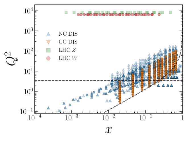
There are several interesting observations that one can make regarding Fig. 2.1. First of all, the LHC proton-lead measurements significantly extend the kinematic coverage of the fixed-target DIS reduced cross-sections, both in terms of $x$ and $Q^{2}$. In particular, the LHC data reside at $Q^{2}$ values that are orders of magnitude larger while the coverage in partonic momentum fraction is extended down to $x\simeq 10^{-3}$. Secondly, the CC reduced cross-sections have a similar coverage compared to the NC ones, providing sensitivity to different quark and antiquark combinations across the shared medium- to large-$x$ region. Finally, the kinematics of the LHC W and Z measurements largely overlap. The ability to describe them simultaneously can therefore demonstrate the compatibility between the experimental data and theoretical calculations.

2.2 Theoretical calculations

DIS structure functions.

For the NC DIS structure functions we use the same theoretical settings as in nNNPDF1.0, i.e. the structure functions are evaluated at NLO using APFEL Bertone:2013vaa in the FONLL-B general-mass variable flavor number scheme Forte:2010ta . The value of the strong coupling constant is taken to be the same as in the NNPDF3.1 proton PDF fit, $\alpha_{S}(m_{Z})=0.118$, as well as the charm and bottom mass thresholds $m_{c}=1.51$ GeV and $m_{b}=4.92$ GeV, respectively. The charm PDF is generated perturbatively by the DGLAP evolution equations and is thus absent from the $n_{f}=3$ scheme. Lastly, the structure functions are processed by the APFELgrid Bertone:2016lga fast interpolation tables which allow for efficient evaluations during the PDF fit.

Concerning the CC neutrino reduced cross-sections, most of the theory settings are shared with their NC counterparts. The main difference is that the heavy quark contributions in the CC predictions at NLO are accounted for in the FONLL-A scheme instead to maintain consistency with the proton baseline. Massive $\mathcal{O}\left(\alpha_{s}^{2}\right)$ corrections to charm production in CC DIS have been presented in Ref. Berger:2016inr , and subsequently used to study their impact in the determination of the strange content of the nucleon in Ref. Gao:2017kkx . Further details about the implementation of heavy quark mass corrections in the NNPDF framework for charged-current scattering can be found in Ref. Ball:2011uy .

Hadronic cross-sections.

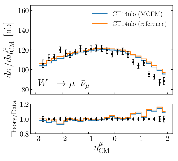
The rapidity distributions from W and Z boson production in proton-lead collisions are evaluated at NLO using MCFM Boughezal:2016wmq v6.8 interfaced with APPLgrid Carli:2010rw . We have ensured that the numerical integration uncertainties in the MCFM calculations are always much smaller than the corresponding experimental errors. Furthermore, our calculations are benchmarked with the reference theoretical values whenever provided by the corresponding experimental publications. To illustrate this benchmarking, we display in Fig. 2.2 the muon rapidity distributions for W^- boson production at $\sqrt{s}=8.16$ TeV in the center-of-mass frame. Here we compare our MCFM-based calculation with the theory predictions provided in Ref. Sirunyan:2019dox at the level of absolute cross-sections (upper panel) and also as ratios to the central experimental values (lower panel). In both cases, the CT14 NLO proton PDF set is adopted as input and nuclear corrections are neglected. As can been seen by the figure, there is good agreement at the $\sim$1% level between our calculations and the reference results provided in the CMS paper. Similar agreement is obtained for the rest of hadronic datasets included in the present analysis.

Figure 2.2: The leptonic rapidity distributions for W^- boson production at $\sqrt{s}=8.16$ TeV in the center-of-mass frame. Our MCFM-based calculation is compared with the theory predictions provided in Sirunyan:2019dox both as absolute cross-sections (upper) and as ratios to the experimental data (lower panel). In both cases the CT14 NLO proton PDF set is adopted and nuclear corrections are neglected.

Since the fast interpolation grids are computed in the center-of-mass frame of the proton-lead collision, rapidity bins that are given in the laboratory frame $\eta_{\rm lab}$ are shifted to the center-of-mass frame $\eta_{\rm CM}$ when required. This shift is given by $\eta_{\rm lab}=\eta_{\rm CM}+0.465$ both at $\sqrt{s}=5.02$ and 8.16 center-of-mass energies. Lastly, we note that the same theoretical settings were used for the evaluation of W and Z production in proton-proton collisions for the baseline NNPDF3.1 fit.

3 Fitting methodology

In this section, we describe the fitting methodology that was adopted for the nNNPDF2.0 determination, focusing in particular on the differences and improvements with respect to the nNNPDF1.0 analysis. We begin by establishing the PDF notation and conventions that will be used throughout this work. We then detail our strategy to parameterize the nuclear parton distributions, including the treatment of sum rules, preprocessing factors, and the proton boundary condition. Lastly, we outline the implementation of the cross-section positivity constraint.

3.1 Notation and conventions

Parton distributions can be parametrized in a number of different bases, all of which are related by linear transformations. Two popular ones are the flavor basis, corresponding to the individual quark and anti-quark PDFs, and the evolution basis, given by the eigenvectors of the DGLAP evolution equations Ball:2014uwa . For illustrative purposes we consider here three active quarks, a vanishing strangeness asymmetry, and heavy quark PDFs that are generated via perturbative evolution. At the parameterization scale $Q_{0}<m_{c}$, the flavor basis is composed of the $u,\,\bar{u},\,d,\,\bar{d},\,s,\,$ and $g$ PDFs, with $s=\bar{s}$, while the corresponding evolution basis is given by $\Sigma,\,T_{3},\,T_{8},\,V,\,V_{3},$ and $g$. Expressed in terms of the elements of the flavor basis, the evolution basis distributions are given by

$$\Sigma(x,Q_{0}) = \left(u^{+}+d^{+}+s^{+}\right)(x,Q_{0})\,,$$

$$T_{3}(x,Q_{0}) = \left(u^{+}-d^{+}\right)(x,Q_{0})\,,$$

$$T_{8}(x,Q_{0}) = \left(u^{+}+d^{+}-2s^{+}\right)(x,Q_{0})\,,$$ (3.1)

$$V(x,Q_{0}) = \left(u^{-}+d^{-}\right)(x,Q_{0})\,,$$

$$V_{3}(x,Q_{0}) = \left(u^{-}-d^{-}\right)(x,Q_{0})\,,$$

where $q^{\pm}=q\pm\bar{q}$. Although the results of an nPDF analysis should be independent of the basis choice for the parameterization, some bases offer practical advantages, for example in the implementation of the sum rules which are discussed later.

In this work, we define $f^{(N/A)}$ to be the PDF for the flavor $f$ associated to the average nucleon $N$ bound in a nucleus with atomic number $Z$ and mass number $A$. This object can be written as

$$f^{(N/A)}(x,Q_{0})={{Z}\over{A}}f^{(p/A)}(x,Q_{0})+\left(1-{{Z}\over{A}}\right)f^{(n/A)}(x,Q_{0})\,,$$ (3.2)

where $f^{(p/A)}$ and $f^{(n/A)}$ represent the PDFs of a proton and a neutron, respectively, bound in the same nucleus of mass number $A$. Assuming isospin symmetry, the PDFs of the neutron in Eq. (3.2) can be expressed in terms of the proton PDFs via

$$u^{(n/A)}(x,Q_{0})=d^{(p/A)}(x,Q_{0})\,,\quad \bar{u}^{(n/A)}(x,Q_{0})=\bar{d}^{(p/A)}(x,Q_{0})$$

$$d^{(n/A)}(x,Q_{0})=u^{(p/A)}(x,Q_{0})\,,\quad \bar{d}^{(n/A)}(x,Q_{0})=\bar{u}^{(p/A)}(x,Q_{0})$$ (3.3)

$$s^{(n/A)}(x,Q_{0})=s^{(p/A)}(x,Q_{0})\,,\quad g^{(n/A)}(x,Q_{0})=g^{(p/A)}(x,Q_{0})\,.$$

Using the relations above, the strange and gluon distributions of the average bound nucleon ($f^{(N/A)}$) and bound proton ($f^{(p/A)}$) become equivalent, while the up and down flavored distributions of the average bound nucleon are instead linear combinations of the bound proton PDFs with coefficients depending on the values of $A$ and $Z$.

3.2 nPDF parameterization

The cross-sections for hard scattering processes involving heavy nuclei can be expressed either in terms of $f^{(N/A)}$ or $f^{(p/A)}$. The two options are fully equivalent, as is highlighted by the LO expressions of the observables collected in Appendix A. One can therefore choose to parameterize either the PDFs of the average bound nucleon or those of the bound proton in a global nPDF analysis. In this study we choose the latter option for two main reasons. First, the connection with the free-proton boundary condition is more straightforward. In addition, the valence sum rules for non-isoscalar nuclei are independent of $A$ and $Z$. If instead $f^{(N/A)}$ is parameterized, one of the valence sum rules would depend on the value of the $Z/A$ ratio and thus be different for each nuclei, making it inconvenient from the parameterization point of view.

The relation between $f^{(N/A)}$ and $f^{(p/A)}$ is trivial also for PDF combinations that comprise the evolution basis. Consider for example the total quark singlet, where the flavor combination is the same in the proton and in the neutron, i.e. $\Sigma^{(p/A)}=\Sigma^{(n/A)}$. From Eq. (3.2), it simply follows that $\Sigma^{(N/A)}=\Sigma^{(p/A)}$. The same equivalence holds also for $V$ and $T_{8}$. However, the distinction is important for $T_{3}$ and $V_{3}$, for which we have

$$V_{3}^{(N/A)}={{Z}\over{A}}V_{3}^{(p/A)}+\left(1-{{Z}\over{A}}\right)V_{3}^{(n/A)}=\left({{2Z}\over{A}}-1\right)V_{3}^{(p/A)}\,,$$ (3.4)

$$T_{3}^{(N/A)}={{Z}\over{A}}T_{3}^{(p/A)}+\left(1-{{Z}\over{A}}\right)T_{3}^{(n/A)}=\left({{2Z}\over{A}}-1\right)T_{3}^{(p/A)}\,,$$ (3.5)

so there is an overall rescaling factor of $(2Z/A-1)$ between $f^{(N/A)}$ and $f^{(p/A)}$. The main consequence of this relation is highlighted by assuming an isoscalar nucleus, with $Z=A/2$. In this case, $V_{3}^{(N/A)}=T_{3}^{(N/A)}=0$ while their bound proton counterparts are different from zero. Unless otherwise indicated, the nPDFs discussed in this section will always correspond to those of the bound proton.

Fitting basis and functional form.

In our previous nNNPDF1.0 analysis, we parameterized only three independent evolution basis distributions at the initial scale $Q_{0}$, namely the total quark singlet $\Sigma(x,Q_{0})$, the quark octet $T_{8}(x,Q_{0})$, and the gluon nPDF $g(x,Q_{0})$. From the LO expression of Eq. (A.5), it is clear that NC structure functions are sensitive only to a specific combination of $\Sigma$ and $T_{8}$ for isoscalar nuclei, in particular $\Sigma+T_{8}/4$, while the contribution proportional to $T_{3}$ vanishes. In other words, $\Sigma$ and $T_{8}$ are strongly anti-correlated and only the combination $\Sigma+T_{8}/4$ can be meaningfully determined from the data.

The picture is quite different in the present study, where the availability of charged current DIS data and electroweak gauge boson production cross-sections in proton-lead collisions allow additional elements of the evolution PDF basis to be parameterized (see App. A). If non-isoscalar effects are neglected, there is only a single distribution to be added to our evolution basis choice, namely the total valence quark combination $V=u^{-}+d^{-}$. However, non-isoscalar corrections are necessary for the targets considered in this analysis, particularly for lead. In this case, the quark triplet $T_{3}=u^{+}-d^{+}$ and the valence triplet $V_{3}=u^{-}-d^{-}$ must also be parameterized. Note that since $T_{3}$ and $V_{3}$ correspond to bound protons, they will be different from zero even for isoscalar nuclei. However, in such cases their contribution to the scattering cross-section vanishes and therefore the data provides no constraint on these combinations.

Putting together these considerations, in this work we parameterize six independent PDF combinations in the evolution basis as follows

$$x\Sigma^{(p/A)}(x,Q_{0}) = x^{\alpha_{\Sigma}}(1-x)^{\beta_{\Sigma}}{\rm NN}_{\Sigma}(x,A)\,,$$

$$xT_{3}^{(p/A)}(x,Q_{0}) = x^{\alpha_{T_{3}}}(1-x)^{\beta_{T_{3}}}{\rm NN}_{T_{3}}(x,A)\,,$$

$$xT_{8}^{(p/A)}(x,Q_{0}) = x^{\alpha_{T_{8}}}(1-x)^{\beta_{T_{8}}}{\rm NN}_{T_{8}}(x,A)\,,$$ (3.6)

$$xV^{(p/A)}(x,Q_{0}) = B_{V}x^{\alpha_{V}}(1-x)^{\beta_{V}}{\rm NN}_{V}(x,A)\,,$$

$$xV_{3}^{(p/A)}(x,Q_{0}) = B_{V_{3}}x^{\alpha_{V_{3}}}(1-x)^{\beta_{V_{3}}}{\rm NN}_{V_{3}}(x,A)\,,$$

$$xg^{(p/A)}(x,Q_{0}) = B_{g}x^{\alpha_{g}}(1-x)^{\beta_{g}}{\rm NN}_{g}(x,A)\,.$$

In these expressions, ${\rm NN}_{f}(x,A)$ stands for the value of the neuron in the output layer of the neural network associated to each specific distribution. As was done in nNNPDF1.0, we use a single artificial neural network consisting of an input layer, one hidden layer with sigmoid activation function, and an output layer with linear activation function. The input layer contains three neurons that take as input the values of the momentum fraction $x$, $\ln(1/x)$, and atomic mass number $A$, respectively. Since the hidden layer contains 25 neurons, there are a total of $N_{\rm par}=256$ free parameters (weights and thresholds) in the neural network used to model our nPDFs.

The neural-net parameterization in Eq. (3.6) is then complemented by three normalization coefficients $B_{g}$, $B_{V}$, and $B_{V_{3}}$ which are fixed by the sum rules, and by twelve preprocessing exponents $\alpha_{f}$ and $\beta_{f}$ which are fitted simultaneously with the network parameters. Since our proton baseline is a variant of the NNPDF3.1 global NLO fit Ball:2017nwa with perturbative charm, we adopt for consistency the same parameterization scale of $Q_{0}=1$ GeV.

It is important to emphasize here that the parameterization in Eq. (3.6) is valid from $A=1$ (free-proton) up to $A=208$ (lead). As a result, the nNNPDF2.0 analysis incorporates an independent determination of the free-proton PDFs, where agreement with the proton PDF baseline is enforced by means of a boundary condition as explained below. This is a relevant distinction, implying that the $A=1$ PDF can by construction differ slightly from our proton baseline, for example as a result of positivity constraints that are more general in the former case, or by new information contained in the LHC proton-lead cross-sections.

Sum rules.

For every nuclei, we assume that the fitted nuclear PDFs satisfy the same valence and momentum sum rules as in the proton case. The sum rules are implemented via an overall normalization factor in the PDF parameterization, which are adjusted each time the neural network parameters are modified in order to ensure that the sum rules remain satisfied. Note that these sum rules need only to be applied at the input scale $Q_{0}$, since the properties of DGLAP perturbative evolutions guarantee that they will also be satisfied for other $Q>Q_{0}$. First, energy conservation leads to the momentum sum rule constraint,

$$\int_{0}^{1}dx\,x\left(\Sigma^{(p/A)}(x,Q_{0})+g^{(p/A)}(x,Q_{0})\right)=1\,,\quad\forall\,A\,,$$ (3.7)

which is enforced by fixing the gluon normalization to be

$$B_{g}(A)={{1-\int_{0}^{1}dx\,x\Sigma^{(p/A)}(x,Q_{0})}\over{\int_{0}^{1}dx\,xg^{(p/A)}(x,Q_{0})}}\,,$$ (3.8)

where the denominator of Eq. (3.8) is evaluated using Eq. (3.6) and setting $B_{g}=1$. Our nuclear PDFs are also constructed to comply with the three valence sum rules that follow from the valence quark quantum numbers of the proton:

$$\int_{0}^{1}dx\leavevmode\nobreak\ \left(u^{(p/A)}(x,Q_{0})-\bar{u}^{(p/A)}(x,Q_{0})\right)=2\,,\quad\forall\,A\,,$$ (3.9)

$$\int_{0}^{1}dx\leavevmode\nobreak\ \left(d^{(p/A)}(x,Q_{0})-\bar{d}^{(p/A)}(x,Q_{0})\right)=1\,,\quad\forall\,A\,,$$ (3.10)

$$\int_{0}^{1}dx\leavevmode\nobreak\ \left(s^{(p/A)}(x,Q_{0})-\bar{s}^{(p/A)}(x,Q_{0})\right)=0\,,\quad\forall\,A\,,$$ (3.11)

where the final relation is trivially satisfied due to our inherent flavor assumption of $s=\bar{s}$.

To implement the former two valence sum rules in our analysis, we first must derive the corresponding constraints in the evolution basis. Adding Eqns. (3.9) and (3.10) results in

$$\int_{0}^{1}dx\leavevmode\nobreak\ \left(u^{(p/A)}(x,Q_{0})-\bar{u}^{(p/A)}(x,Q_{0})+d^{(p/A)}(x,Q_{0})-\bar{d}^{(p/A)}(x,Q_{0})\right)=$$

$$\int_{0}^{1}dx\leavevmode\nobreak\ V^{(p/A)}(x,Q_{0})=3\,,\quad\forall\,A\,.$$ (3.12)

This condition can then be implemented in the same way as the momentum sum rule, namely by setting the overall normalization factor of $V$ as

$$B_{V}(A)={{3}\over{\int_{0}^{1}dx\,V^{(p/A)}(x,Q_{0},A)}}\,,$$ (3.13)

where the denominator of Eq. (3.13) is evaluated using Eq. (3.6) and setting $B_{V}=1$.

The second valence sum rule in the evolution basis is the one related to the quark valence triplet $V_{3}$. Subtracting Eq. (3.10) from (3.9) gives

$$\int_{0}^{1}dx\leavevmode\nobreak\ \left(u^{(p/A)}(x,Q_{0},A)-\bar{u}^{(p/A)}(x,Q_{0},A)-d^{(p/A)}(x,Q_{0},A)+\bar{d}^{(p/A)}(x,Q_{0},A)\right)=$$

$$\int_{0}^{1}dx\leavevmode\nobreak\ V_{3}^{(p/A)}(x,Q_{0},A)=1\,,\quad\forall\,A\,.$$ (3.14)

which again is imposed by setting

$$B_{V_{3}}(A)={{1}\over{\int_{0}^{1}dx\,V_{3}^{(p/A)}(x,Q_{0},A)}}\,,$$ (3.15)

where the denominator of Eq. (3.15) is evaluated using Eq. (3.6) with $B_{V_{3}}=1$.

In this analysis, the normalization pre-factors $B_{g}(A)$, $B_{V}(A)$, and $B_{V_{3}}(A)$ are computed using the trapezoidal rule for numerical integration between $x_{\rm min}=10^{-9}$ and $x_{\rm max}=1$ each time the fit parameters are updated by the minimization procedure. With a suitable choice of the ranges for the preprocessing exponents (see discussion below), we guarantee that each quark combination satisfies the corresponding physical integrability conditions. Lastly, we have confirmed that individual replicas satisfy the sum rules with a precision of a few per-mille or better.

An interesting question in the context of nuclear global QCD analyses is the extent to which theoretical constraints such as the sum rules are satisfied by the experimental data when not explicitly imposed. In fact, it was shown in Ref. Ball:2011uy that the momentum sum for the free proton agrees with the QCD expectation within $\sim 1\%$ in this scenario. Here we will revisit this analysis for the nuclear case, and will present in Sect. 4.3 variants of the nNNPDF2.0 fit where either the momentum sum rule, Eq. (3.7), or the valence sum rule, Eq. (3.2), is not enforced. Interestingly, we will find that the experimental data is in agreement with sum rule expectations, albeit within larger uncertainties, demonstrating the remarkable consistency of the nuclear global QCD analysis.

Preprocessing exponents.

The $x^{\alpha_{f}}(1-x)^{\beta_{f}}$ polynomial pre-factors appearing in Eq. (3.6) are included to increase the efficiency of the parameter optimization, since they approximate the general PDF behavior in the small- and large-$x$ asymptotic limits Ball:2016spl . Note that the exponents $\alpha_{f}$ and $\beta_{f}$ are $A$-independent, implying that $A$ dependence of the nPDFs will arise completely from the output of the neural network. As in the case of the nNNPDF1.0 analysis, the values of $\alpha_{f}$ and $\beta_{f}$ are fitted for each Monte Carlo replica on the same footing as the weights and thresholds of the neural network.

The ranges of the preprocessing parameters are determined both by physical considerations and by empirical observations. First of all, the lower limit of the small-$x$ parameter is set so that each PDF combination satisfies various integrability conditions. In particular, the non-singlet combinations $xV$, $xV_{3}$, $xT_{3}$, and $xT_{8}$ must tend to zero at small-$x$, else the valence sum rules and other relations such as the Gottfried sum rule Forte:1992df ; Abbate:2005ct would be ill-defined. Moreover, the singlet combinations $x\Sigma$ and $xg$ must be exhibit finite integrable behavior as $x\rightarrow 0$, otherwise the momentum integral cannot be computed. Concerning the large-$x$ exponents $\beta_{f}$, the lower limits of their ranges ensure that PDFs vanish in the elastic limit, while the upper limit is determined largely from general arguments related to sum rule expectations. In general, however, the upper values of both $\alpha_{f}$ and $\beta_{f}$ are chosen to be sufficiently large to allow flexibility in exploring the parameter space while keeping fit efficiency optimal.

Under these considerations, we restrict the parameter values for the pre-processing factors during the fit to the following intervals,

$$\alpha_{\Sigma} \in[-1,5]\leavevmode\nobreak\ \leavevmode\nobreak\ ([-1,1])\,, \beta_{\Sigma} \in[1,10]\leavevmode\nobreak\ \leavevmode\nobreak\ ([1,5])\,,$$

$$\alpha_{g} \in[-1,5]\leavevmode\nobreak\ \leavevmode\nobreak\ ([-1,1])\,, \beta_{g} \in[1,10]\leavevmode\nobreak\ \leavevmode\nobreak\ ([1,5])\,,$$

$$\alpha_{V} \in[0,5]\leavevmode\nobreak\ \leavevmode\nobreak\ ([1,2])\,, \beta_{V} \in[1,10]\leavevmode\nobreak\ \leavevmode\nobreak\ ([1,5])\,,$$ (3.16)

$$\alpha_{T_{8}} \in[-1,5]\leavevmode\nobreak\ \leavevmode\nobreak\ ([-1,1])\,, \beta_{T_{8}} \in[1,10]\leavevmode\nobreak\ \leavevmode\nobreak\ ([1,5])\,,$$

$$\alpha_{V_{3}} \in[0,5]\leavevmode\nobreak\ \leavevmode\nobreak\ ([1,2])\,, \beta_{V_{3}} \in[1,10]\leavevmode\nobreak\ \leavevmode\nobreak\ ([1,5])\,,$$

$$\alpha_{T_{3}} \in[-1,5]\leavevmode\nobreak\ \leavevmode\nobreak\ ([-1,1])\,, \beta_{T_{3}} \in[1,10]\leavevmode\nobreak\ \leavevmode\nobreak\ ([1,5])\,,$$

where the ranges in parentheses are those used to randomly select the initial values of $\alpha_{f}$ and $\beta_{f}$ at the start of the minimization. We do not impose any specific relation between the small- or large-$x$ exponents of the different quark combinations, so that each are fitted independently. It is also worth emphasizing here that the neural network has the ability to compensate for any deviations in the shape of the preprocessing function, so the dependence on $x$ and $A$ of the nPDFs in the data region will be dominated by the neural network output. This implies that the preprocessing exponents will primarily affect the results in the extrapolation regions.

Figure 3.1: Same as Fig. 3.2 for the fitted small-$x$ preprocessing exponents $\alpha_{f}$

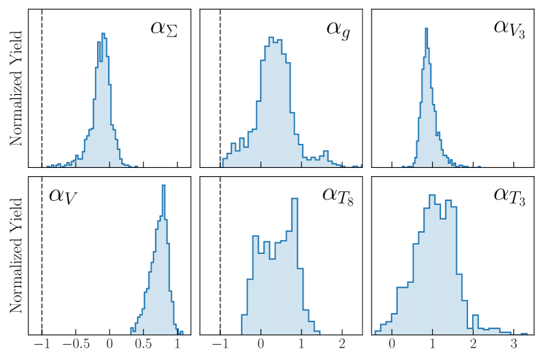
To illustrate the values of the small and large-$x$ preprocessing exponents preferred by the experimental data, we display in Figs. 3.1 and 3.2 the probability distributions associated with the $\alpha_{f}$ and $\beta_{f}$ exponents, respectively, computed using the $N_{\rm rep}=1000$ replicas of the nNNPDF2.0 analysis. Note how these exponents are restricted to lie in the interval given by Eq. (3.2). For $T_{3}$ and $T_{8}$, we can see that despite not imposing the strict integrability requirement that $\alpha_{f}>0$, it is still being satisfied for a large majority of the replicas, especially for $T_{3}$. Interestingly, the gluon seems to prefer a valence-like behavior at small-$x$. However, such behaviour is only observed at the parameterization scale and as soon as $Q>Q_{0}$, DGLAP evolution drives it to its expected singlet-like behavior.

Figure 3.2: The probability distribution associated to the fitted large-$x$ preprocessing exponents $\beta_{f}$ computed with the $N_{\rm rep}=1000$ replicas of the nNNPDF2.0 NLO set. The ranges for which these exponents are allowed to vary, Eq. (3.2), are indicated by horizontal dashed lines.

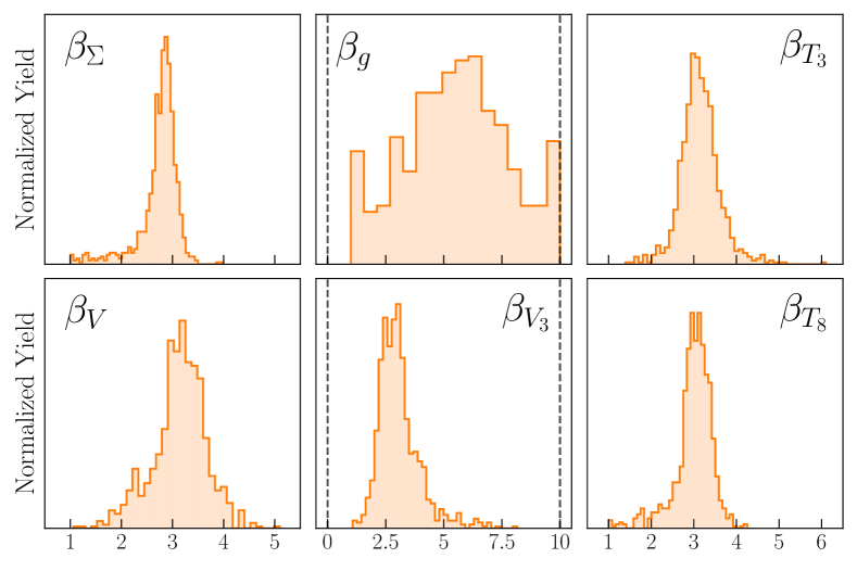
Concerning the behavior of the large-$x$ exponents $\beta_{f}$, we find that they are reasonably well constrained for the quark distributions, where the best-fit values are located in a region close to $\beta_{f}\simeq 3$. The fact that they share similar $\beta_{f}$ exponents can be explained by the fact that in the large-$x$ region the quark combinations are dominated by valence components. Interestingly, a best-fit value of $\beta_{f}\simeq 3$ for the valence quarks is consistent with the expectations from the QCD counting rules, as discussed in Ball:2016spl . Furthermore, the best-fit value for $\beta_{g}$ is also consistent with the QCD counting rules prediction of $\beta_{g}\simeq 5$, although with significant uncertainties. The fact that $\beta_{g}$ is found to vary in a wide range is due to the lack of direct constraints on the large-$x$ nuclear gluon PDF in the present analysis.

The free-proton boundary condition.

As was done in our previous study, we again implement the condition that the proton PDF baseline, obtained with consistent theoretical and methodological choices, is reproduced when $A\rightarrow 1$. This condition should be constructed to match the free-proton distributions not only in terms of central values but also at the level of PDF uncertainties. In other words, it should allow a full propagation of the information contained in the proton baseline, which is particularly important to constrain the nPDFs of relatively light nuclei. Note, however, that for the reasons explained above, the nNNPDF2.0 $A=1$ set will in general not be strictly identical to the corresponding proton baseline.

The proton boundary condition constraint is implemented by adding a quadratic penalty term to the $\chi^{2}$ of the form

$$\chi^{2}\to\chi^{2}+\lambda_{\rm BC}\sum_{f}\sum_{i=1}^{N_{x}}\left(q_{f}^{(p/A)}(x_{i},Q_{0},A=1)-q_{f}^{(p)}(x_{i},Q_{0})\right)^{2}\,,$$ (3.17)

where the sum over flavors $f$ runs over the six independent elements in the PDF evolution basis. Since the properties of DGLAP evolution ensure that the distributions for $Q>Q_{0}$ also satisfy the condition, only the PDFs at the parameterization scale $Q_{0}$ enter the penalty term. In Eq. (3.17), we use a grid with $N_{x}=60$ points of which 10 are distributed logarithmically from $x_{\rm min}=10^{-3}$ to $x_{\rm mid}=0.1$ and the remaining 50 points are linearly distributed from $x_{\rm mid}=0.1$ to $x_{\rm max}=0.7$. The value of the boundary condition hyper-parameter is fixed to be $\lambda_{\rm BC}=100$ as was done in the previous nNNPDF1.0 analysis. For such a value, we find that the central values and uncertainties of the proton baseline are reasonably well described (see Sect. 4).

In this analysis the proton baseline, $f^{(p)}(x,Q_{0})$, is taken to be a variant of the NNPDF3.1 NLO fit Ball:2017nwa with perturbative charm, where the neutrino DIS cross-sections from NuTeV and CHORUS are removed along with the di-muon production measurements in proton-copper collisions from the E605 experiment Moreno:1990sf . As such, the proton baseline not only avoids double counting of the CC DIS data but also excludes constraints from heavy nuclear target data where nuclear effects are neglected. This choice is different to that used for nNNPDF1.0, where the global NNPDF3.1 fit was used and double-counting of experimental data was not an issue.

Figure 3.3: A comparison between the global NNPDF3.1 free-proton analysis with its variant with heavy nuclear data excluded. We show results for the up quark, down antiquark, total strangeness, and the gluon at $Q_{0}=1$ GeV. The comparison is presented for the range of $x$ for which the proton boundary condition is implemented in nNNPDF2.0 using Eq. (3.17). The PDF uncertainty bands correspond to 90% CL intervals.

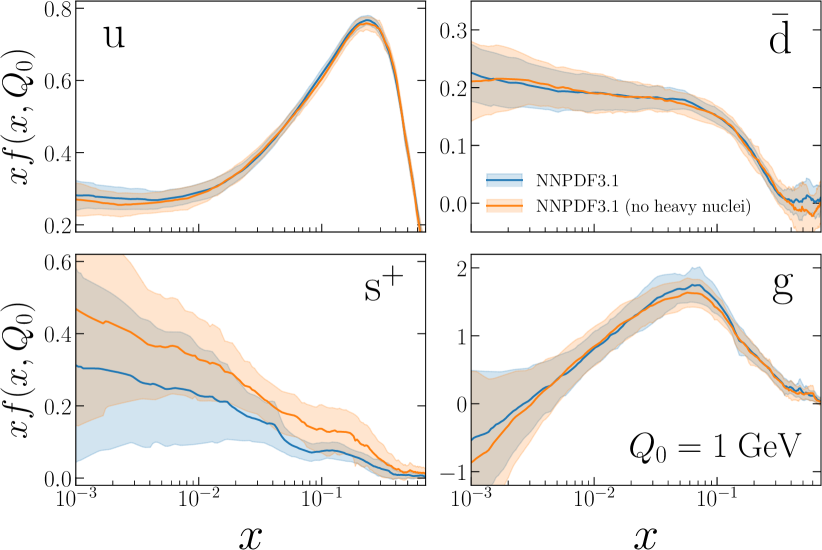
In order to illustrate the differences between the free-proton boundary condition used in nNNPDF1.0 and that employed in the present analysis, we compare in Fig. 3.3 the NNPDF3.1 NLO global and no heavy nuclear fits at the initial parameterization scale of $Q_{0}=1$ GeV. Displayed are the gluon, up quark, down sea quark, and total strange PDFs in the range of $x$ with which the proton boundary condition is constrained by Eq. (3.17). Here one can see that removing the heavy nuclear data from NNPDF3.1 results in a moderate increase of the PDF uncertainties associated to the quarks as well as an upward shift of the central value of the total strange distribution. The former effect is primarily a consequence of information loss on quark flavor separation with the removal of neutrino scattering measurements. The strangeness feature, on the other hand, arises due to the absence of sensitivity from the NuTeV neutrino dimuon cross-sections, resulting in an upward pull by the ATLAS $W,Z$ 2011 rapidity distributions which are known to produce an enhanced strange with respect to the up and down quark sea. The results of Fig. 3.3 highlight the importance of a consistent choice of the free-proton baseline in order to draw solid conclusions on the nuclear modifications, for example those associated to the nucleon’s strange content.

In order to ensure that all central values and PDF uncertainties are reproduced, we select a different replica from the NNPDF3.1 proton baseline when constructing Eq. (3.17) for each replica of nNNPDF2.0. Since we perform a large $N_{\rm rep}$ number of fits to estimate the uncertainties in nNNPDF2.0, we are able to propagate the necessary information contained in NNPDF3.1 to the resulting nPDFs in a robust manner. Lastly, we note that Eq. (3.17) is the only place in the analysis where the free-proton NNPDF3.1 baseline is inserted. In other parts of the fit where a free-nucleon PDF is required, for example in the theoretical predictions of the proton-lead scattering cross-sections, the nNNPDF2.0 set with $A=1$ is used instead.

3.3 Cross-section positivity

While parton distributions are scheme-dependent and thus not necessarily positive-definite beyond leading order in perturbative QCD, physical cross-sections constructed from them are scheme independent and should be positive-definite in the region of validity of the perturbative expansion. In the NNPDF family of proton PDF fits, the requirement that cross-sections remain positive is implemented by adding to the $\chi^{2}$ a penalty term in the presence of negative cross-section values Ball:2014uwa . The cross-sections that enter this penalty term correspond to theoretical predictions based on pseudo-data generated for representative processes that are directly sensitive to a sufficient number of PDF combinations.

In the nNNPDF1.0 analysis, cross-section positivity was not imposed and led to some observables, such as the longitudinal structure function $F_{L}(x,Q^{2})$, becoming negative at small-$x$ values outside the data region. To bypass this problem, and also to improve the methodological consistency with the free-proton baseline, in nNNPDF2.0 we impose the positivity of physical cross-sections for all nuclei used in the fit by adding a suitable penalty to the figure of merit. In this case, the positivity penalty is expressed as

$$\chi^{2}\to\chi^{2}+\lambda_{\rm pos}\sum_{l=1}^{N_{\rm pos}}\sum_{j=1}^{N_{A}}\sum_{i_{l}=1}^{N_{\rm dat}^{(l)}}{\rm max}\left(0,-\mathcal{F}_{i_{l}}^{(l)}(A_{j})\right)\,,$$ (3.18)

for $N_{\rm pos}$ positivity observables $\mathcal{F}^{(l)}$. Each of the observables contain $N_{\rm dat}^{(l)}$ kinematic points that are chosen to cover an adequately large region of phase space relevant to various PDF combinations, as we discuss in more detail below. The computed observables are summed over all $N_{A}$ nuclei for which we have experimental data, as listed in Tables 2.1 and 2.2, as well as for the free-proton at $A=1$. Finally, the value of the hyper-parameter $\lambda_{\rm pos}=1000$ is determined by manual inspection of the optimization process and is chosen so that positivity is satisfied without distorting the training on the real experimental data.

Observable	LO expression	$N_{\rm dat}$	Kinematic coverage
$F_{2}^{u}(x,Q^{2},A)$	$\propto\left(u^{N/A}+\bar{u}^{N/A}\right)$	20	$Q^{2}=5$ GeV
	$\propto\left[(Z/A)\left(u^{p/A}+\bar{u}^{p/A}\right)+(1-Z/A)\left(d^{p/A}+\bar{d}^{p/A}\right)\right]$		$5\times 10^{-7}\leq x\leq 0.9$
$F_{2}^{d}(x,Q^{2},A)$	$\propto\left(d^{N/A}+\bar{d}^{N/A}\right)$	20	$Q^{2}=5$ GeV
	$\propto\left[(Z/A)\left(d^{p/A}+\bar{d}^{p/A}\right)+(1-Z/A)\left(u^{p/A}+\bar{u}^{p/A}\right)\right]$		$5\times 10^{-7}\leq x\leq 0.9$
$F_{2}^{s}(x,Q^{2},A)$	$\propto\left(s^{N/A}+\bar{s}^{N/A}\right)$	20	$Q^{2}=5$ GeV
	$\propto\left(s^{p/A}+\bar{s}^{p/A}\right)$		$5\times 10^{-7}\leq x\leq 0.7$
$F_{L}(x,Q^{2},A)$	sensitive to $xg(x,Q^{2})$ (see text)	20	$Q^{2}=5$ GeV
			$5\times 10^{-7}\leq x\leq 0.9$
$\sigma_{u\bar{u}}^{DY}(y,M^{2},A)$	$\propto\left(u^{p}(x_{1})\times\bar{u}^{N/A}(x_{2})\right)$	20	$Q^{2}=5$ GeV
	$\propto\left(u^{p}(x_{1})\times\left(Z\bar{u}^{p/A}(x_{2})+(A-Z)\bar{d}^{p/A}(x_{2})\right)\right)$		$10^{-2}\leq x\leq 0.9$
$\sigma_{d\bar{d}}^{DY}(y,M^{2},A)$	$\propto\left(d^{p}(x_{1})\times\bar{d}^{N/A}(x_{2})\right)$	20	$Q^{2}=5$ GeV
	$\propto\left(d^{p}(x_{1})\times\left(Z\bar{d}^{p/A}(x_{2})+(A-Z)\bar{u}^{p/A}(x_{2})\right)\right)$		$10^{-2}\leq x\leq 0.9$
$\sigma_{s\bar{s}}^{DY}(y,M^{2},A)$	$\propto\left(s^{p}(x_{1})\times\bar{s}^{N/A}(x_{2})\right)$	20	$Q^{2}=5$ GeV
	$\propto\left(s^{p}(x_{1})\times\bar{s}^{p/A}(x_{2})\right)$		$10^{-2}\leq x\leq 0.9$
$\sigma_{\bar{u}d}^{DY}(y,M^{2},A)$	$\propto\left(\bar{u}^{p}(x_{1})\times d^{N/A}(x_{2})\right)$	20	$Q^{2}=5$ GeV
	$\propto\left(\bar{u}^{p}(x_{1})\times\left(Zd^{p/A}(x_{2})+(A-Z)u^{p/A}(x_{2})\right)\right)$		$10^{-2}\leq x\leq 0.9$
$\sigma_{\bar{d}u}^{DY}(y,M^{2},A)$	$\propto\left(\bar{d}^{p}(x_{1})\times u^{N/A}(x_{2})\right)$	20	$Q^{2}=5$ GeV
	$\propto\left(\bar{d}^{p}(x_{1})\times\left(Zu^{p/A}(x_{2})+(A-Z)d^{p/A}(x_{2})\right)\right)$		$10^{-2}\leq x\leq 0.9$
$\sigma_{u\bar{s}}^{DY}(y,M^{2},A)$	$\propto\left(u^{p}(x_{1})\times\bar{s}^{N/A}(x_{2})\right)$	20	$Q^{2}=5$ GeV
	$\propto\left(u^{p}(x_{1})\times\bar{s}^{p/A}(x_{2})\right)$		$10^{-2}\leq x\leq 0.9$
$\sigma_{\bar{u}s}^{DY}(y,M^{2},A)$	$\propto\left(\bar{u}^{p}(x_{1})\times s^{N/A}(x_{2})\right)$	20	$Q^{2}=5$ GeV
	$\propto\left(\bar{u}^{p}(x_{1})\times s^{p/A}(x_{2})\right)$		$10^{-2}\leq x\leq 0.9$

Table 3.1: The processes used to impose the positivity of physical cross-sections by means of the constraint of Eq. (3.18). For each process we indicate the corresponding LO expressions, the number of data points $N_{\rm dat}$, and the kinematic coverage spanned by the pseudo-data.

In Table 3.1 we list the $\mathcal{F}^{(l)}$ processes used in this analysis for which the positivity of physical cross-sections is imposed using Eq. (3.18). For each observable, the LO expressions in terms of the average bound nucleon PDFs and bound proton distributions are given together with the number of pseudo-data points $N_{\rm dat}$ and the corresponding kinematic coverage. Note that the LO expressions in Table 3.1 are shown for illustration purposes only, and in our analysis these observables are computed using the full NLO formalism.

Here we consider two types of positivity observables. The first type are the DIS structure functions $F_{2}^{u}$, $F_{2}^{d}$, $F_{2}^{s}$, and $F_{L}$. The former three quantities, which contain only $u$, $d$, and $s$ contributions, respectively, are constructed to be positive-definite since there exists consistent physical theories where the photon couples only to up-, down-, or strange-type quarks. The longitudinal structure function $F_{L}$, on the other hand, largely impacts the nuclear gluon PDF since $F_{L}$ enters only at NLO and is dominated by the gluon contribution. Lastly, we evaluate each of these structure functions on a grid of $N=20$ pseudo-data points between $x=10^{-7}$ and $x=0.9$ at $Q=\sqrt{5}$ GeV, which is slightly above the input parameterization scale $Q_{0}=1$ GeV to ensure perturbative stability.

The second type of observable for which the cross-section positivity is imposed is the double-differential Drell-Yan cross-section. In particular, we enforce the positivity of both neutral- and charged-current Drell-Yan cross-sections in pA scattering for specific combinations of quark-antiquark annihilation listed in Table 3.1. At leading order, the Drell-Yan cross-section can be written schematically as

$${{d^{2}\sigma_{q_{f_{1}}\bar{q}_{f_{2}}}^{DY}}\over{dydQ^{2}}}\propto\left(f_{1}^{(p)}(x_{1},Q^{2})\bar{f_{2}}^{(p/A)}(x_{2},Q^{2})\right)\,,$$ (3.19)

where the momentum fractions $x_{1}$ and $x_{2}$ are related to the rapidity $y$ and invariant mass of the final state $Q$ at at leading order by $x_{1,2}=\left(Q/\sqrt{s}\right)e^{\pm y}$. Here we set $Q^{2}=5$ GeV² and adjust the rapidity range and center-of-mass energy $\sqrt{s}$ so that the LO kinematic range for $x_{1}$ and $x_{2}$ correspond to $10^{-2}\leq x_{1,2}\leq 0.9$.

Note that positivity of Eq. (3.19) will affect also the fitted nNNPDF2.0 $A=1$ distribution which enters as the free-proton PDF. While most of the positivity observables coincide with those included in the free-proton baseline from which the $A=1$ distribution is derived, the $u\bar{d}$, $\bar{u}d$, $u\bar{s}$, and $\bar{u}s$ combinations of Table 3.1 are new in the nNNPDF2.0 determination. Consequently, we impose these new observables only for proton-iron and proton-lead collisions, the two nuclei for which experimental data from charged-current DIS and Drell-Yan reactions are analyzed to study quark flavor separation.

In Sect. 4.4 we will demonstrate the positivity of cross-sections for all relevant processes in the entire kinematical range. We have verified that, in the absence of these constraints, the DIS structure functions and the DY cross-section will in general not satisfy positivity.

4 Results

In this section we present the main results of this work, namely the nNNPDF2.0 determination of nuclear PDFs. We first study the features of the nNNPDF2.0 fit by assessing the quality of its agreement with experimental data, focusing largely on the LHC weak boson production cross-sections, and by studying the behavior of nuclear modification ratios across different nuclei. Subsequently, we contrast this new nPDF determination with its predecessor, nNNPDF1.0, and trace the origin of observed differences via a series of fits with systematic changes. We then study the role that the valence and momentum sum rules play in the global nPDF determination by presenting two variants of the nNNPDF2.0 fit in which one of the two sum rules is not imposed. Finally, we demonstrate that the nNNPDF2.0 fit satisfies the positivity of physical cross-sections in the kinematic range where experimental data is available.

4.1 The nNNPDF2.0 determination

We begin by discussing the fit quality which is assessed across the various datasets and quantified by the $\chi^{2}$ figure of merit. A comparison is then made using the nNNPDF2.0 predictions with the LHC weak gauge boson production measurements. Following this, we take a closer look on the nNNPDF2.0 parton distributions and the corresponding ratios to the free-nucleon case. Lastly, we investigate the sensitivity of the nuclear modification factors with respect to the atomic mass $A$, in particular on the sea quarks and strangeness, and compare our results with those from the EPPS16 analysis.

Fit quality.

In Tables 4.1 and 4.2 we collect the values of the $\chi^{2}$ per data point for all the datasets included in the nNNPDF2.0 analysis, i.e. the neutral and charged current DIS structure functions as well as gauge boson production measurements at the LHC. We compare the nNNPDF2.0 results with a variant fit where we exclude all LHC datasets (DIS only) and with EPPS16. Values in italics indicate predictions for datasets not included in the corresponding fits. The numbers presented in Tables 4.1 and 4.2 contain only the contribution to the $\chi^{2}$ associated with the experimental data, and do not include penalty from the proton boundary condition or positivity constraint (the latter of which vanishes for all final nNNPDF2.0 replicas anyway). Moreover, while we use the $t_{0}$ prescription Ball:2009qv during the optimization to avoid the D’Agostini bias, the quoted numbers correspond to the experimental definition of the $\chi^{2}$ instead Ball:2012wy , in which the central experimental value is used to compute the correlated multiplicative uncertainties.

		nNNPDF2.0 (DIS)	nNNPDF2.0	EPPS16nlo
Dataset	$n_{\rm dat}$	$\chi^{2}/n_{\rm dat}$	$\chi^{2}/n_{\rm dat}$	$\chi^{2}/n_{\rm dat}$
${\rm NMC\,\,(He/D)}$	13	1.11	1.129	0.829
${\rm SLAC\,\,(He/D)}$	3	0.623	0.638	0.152
${\rm NMC\,\,(Li/D)}$	12	1.083	1.166	0.74
${\rm SLAC\,\,(Be/D)}$	3	1.579	1.719	0.098
${\rm EMC\,\,(C/D)}$	12	1.292	1.321	1.174
${\rm FNAL\,\,(C/D)}$	3	0.932	0.838	0.985
${\rm NMC\,\,(C/D)}$	26	2.002	2.171	0.872
${\rm SLAC\,\,(C/D)}$	2	0.286	0.251	1.075
${\rm BCDMS\,\,(N/D)}$	9	2.439	2.635	n/a
${\rm SLAC\,\,(Al/D)}$	3	0.606	0.864	0.326
${\rm EMC\,\,(Ca/D)}$	3	1.72	1.722	1.82
${\rm FNAL\,\,(Ca/D)}$	3	1.253	1.194	1.354
${\rm NMC\,\,(Ca/D)}$	12	1.503	1.747	1.772
${\rm SLAC\,\,(Ca/D)}$	2	0.82	0.771	1.642
${\rm BCDMS\,\,(Fe/D)}$	16	2.244	2.743	0.765
${\rm EMC\,\,(Fe/D)}$	58	0.827	0.875	0.445
${\rm SLAC\,\,(Fe/D)}$	8	2.171	2.455	1.06
${\rm EMC\,\,(Cu/D)}$	27	0.523	0.572	0.714
${\rm SLAC\,\,(Ag/D)}$	2	0.667	0.691	1.595
${\rm EMC\,\,(Sn/D)}$	8	2.197	2.248	2.265
${\rm FNAL\,\,(Xe/D)}$	4	0.414	0.384	n/a
${\rm SLAC\,\,(Au/D)}$	3	1.216	1.353	1.916
${\rm FNAL\,\,(Pb/D)}$	3	2.243	2.168	2.044
${\rm NMC\,\,(Be/C)}$	14	0.268	0.269	0.27
${\rm NMC\,\,(C/Li)}$	9	1.063	1.117	0.9
${\rm NMC\,\,(Al/C)}$	14	0.345	0.354	0.396
${\rm NMC\,\,(Ca/C)}$	23	0.468	0.44	0.564
${\rm NMC\,\,(Fe/C)}$	14	0.663	0.667	0.751
${\rm NMC\,\,(Sn/C)}$	119	0.607	0.638	0.626
${\rm NMC\,\,(Ca/Li)}$	9	0.259	0.276	0.15

Table 4.1: The values of the $\chi^{2}$ per data point for the DIS neutral current structure function datasets included in nNNPDF2.0. We compare the nNNPDF2.0 global and DIS-only results with those obtained using EPPS16 as input for the theory predictions.

		nNNPDF2.0 (DIS)	nNNPDF2.0	EPPS16nlo
Dataset	$n_{\rm dat}$	$\chi^{2}/n_{\rm dat}$	$\chi^{2}/n_{\rm dat}$	$\chi^{2}/n_{\rm dat}$
${\rm NuTeV\,\,(\bar{\nu}Fe)}$	37	0.946	1.094	0.639
${\rm NuTeV\,\,(\nu Fe)}$	39	0.287	0.264	0.381
${\rm CHORUS\,\,(\bar{\nu}Pb)}$	423	0.938	0.97	1.107
${\rm CHORUS\,\,(\nu Pb)}$	423	1.007	1.015	1.024
${\rm ATLAS^{5TEV}\,\,Z}$	14	1.469	1.134	1.12
${\rm CMS^{5TeV}\,\,W^{-}}$	10	1.688	1.078	0.857
${\rm CMS^{8TeV}\,\,W^{-}}$	24	1.453	0.72	0.825
${\rm CMS^{5TeV}\,\,W^{+}}$	10	2.32	1.125	1.211
${\rm CMS^{8TeV}\,\,W^{+}}$	24	3.622	0.772	0.951
${\rm CMS^{5TeV}\,\,Z}$	12	0.58	0.52	0.639
Total	1467	1.013	0.976	0.896

Table 4.2: Same as Table 4.1 now for the new datasets included in nNNPDF2.0: charged current DIS structure functions and gauge boson production at the LHC. We also provide the values of $\chi^{2}/n_{\rm dat}$ for the total dataset. Values in italics indicate predictions for datasets not included in the corresponding fit.

From the results of Table 4.1 and 4.2, one can see that the nNNPDF2.0 determination achieves a satisfactory description of all datasets included in this analysis. A good $\chi^{2}$ is obtained in particular for the charged-current DIS cross-sections and LHC gauge boson production distributions. For instance, for the precise W boson rapidity distributions at $\sqrt{s}=8.16$ TeV from CMS one finds $\chi^{2}/n_{\rm dat}=0.74$ for $n_{\rm dat}=48$ data points. The corresponding predictions using EPPS16 (which do not include this dataset) also lead to a good agreement with $\chi^{2}/n_{\rm dat}=0.88$. The description of most neutral current DIS datasets is comparable to that of nNNPDF1.0. Some datasets, such as the SLAC iron structure functions, are somewhat deteriorated with respect to nNNPDF1.0, possibly due to some mild tension with the CC cross-sections. Further, we find that our resulting fit quality to the CC deep-inelastic structure functions is similar to that obtained in the corresponding proton PDF analysis Ball:2017nwa .

Overall, the resulting $\chi_{\rm tot}^{2}/n_{\rm dat}=0.976$ for the $n_{\rm dat}=1467$ data points included in the fit highlights the remarkable consistency of the experimental data on nuclear targets and the corresponding theory predictions based on the QCD factorization framework. A similar total $\chi^{2}$ is obtained for the theoretical predictions computed using EPPS16 as input. As will be shown below, the fact that both global fits lead to comparable $\chi^{2}$ values can be explained by the corresponding similarities at the nPDF level.

Comparison with experimental data.

To facilitate our discussion regarding the comparison between data and theory calculations, we first introduce here the conventions that we use to define the nuclear modification factors. Following the notations of Sect. 3.1, the Drell-Yan rapidity distributions in proton-nucleus collision can be expressed as

$${{d\sigma_{\rm DY}(y)}\over{dy}}\equiv A{{d\sigma^{(N/A)}_{\rm DY}(y)}\over{dy}}=Z{{d\sigma^{(p/A)}_{\rm DY}(y)}\over{dy}}+\left(A-Z\right){{d\sigma^{(n/A)}_{\rm DY}(y)}\over{dy}}\,,$$ (4.1)

where the superindices $N/A$, $p/A$, and $n/A$ indicate respectively the collision between a proton with an average nucleon, a proton, or a neutron bound within a nucleus of atomic number $Z$ and mass number $A$. As in the case of the PDFs, the bound proton and nucleon cross-sections $\sigma_{\rm DY}^{(p/A)}$ and $\sigma_{\rm DY}^{(n/A)}$ are related to each other via isospin symmetry.

The expression in Eq. (4.1) helps in emphasizing the two reasons why the Drell-Yan cross-sections will be different between pp and pA collisions. The first is due to the modifications of the bound proton PDFs in nuclei, namely the fact that $\sigma_{\rm DY}^{(p/A)}\neq\sigma_{\rm DY}^{(p)}$. Secondly, the predictions of pA collisions using non-isoscalar nuclei would still differ from those of pp reactions in the absence of nuclear modifications, i.e. $\sigma_{\rm DY}^{(p/A)}=\sigma_{\rm DY}^{(p)}$, as a consequence of the unequal amount of protons and neutrons in the target, resulting in $\sigma_{\rm DY}^{(N/A)}\neq\sigma_{\rm DY}^{(p)}$.

Taking these considerations into account, one should define the nuclear modification factor in Drell-Yan proton-nuclear collisions as

$$R_{A}^{\rm DY}(y)\equiv\left({{d\sigma^{(p/A)}_{\rm DY}(y)}\over{dy}}+\left({{A}\over{Z}}-1\right){{d\sigma^{(n/A)}_{\rm DY}(y)}\over{dy}}\right)\Bigg{/}\left({{d\sigma^{(p)}_{\rm DY}(y)}\over{dy}}+\left({{A}\over{Z}}-1\right){{d\sigma^{(n)}_{\rm DY}(y)}\over{dy}}\right)\,.$$ (4.2)

With the above definition, one should find that $R_{A}^{\rm DY}(y)\neq 1$ only in the presence of genuine nuclear corrections, that is, when $\sigma_{\rm DY}^{(p/A)}\neq\sigma_{\rm DY}^{(p)}$. The definition of Eq. (4.2) differs from that of an observable frequently measured in proton-lead collisions, where the proton-nucleus cross-section is normalized to a proton-proton baseline,

$$R_{A,\rm exp}^{\rm DY}(y) \equiv {{d\sigma^{(N/A)}_{\rm DY}(y)}\over{dy}}\Bigg{/}{{d\sigma^{(p)}_{\rm DY}(y)}\over{dy}}$$

$$= \left({{Z}\over{A}}{{d\sigma^{(p/A)}_{\rm DY}(y)}\over{dy}}+\left(1-{{Z}\over{A}}\right){{d\sigma^{(n/A)}_{\rm DY}(y)}\over{dy}}\right)\Bigg{/}\left({{d\sigma^{(p)}_{\rm DY}(y)}\over{dy}}\right)\,.$$

As explained above, in proton-nuclear collisions one will find $R_{A,\rm exp}^{\rm DY}(y)\neq 1$ for non-isoscalar targets even when $\sigma_{\rm DY}^{(p/A)}=\sigma_{\rm DY}^{(p)}$ due to the imbalance between the number of protons and neutrons. In this section, we will exclusively use the definition of Eq. (4.2) when evaluating the theoretical predictions of nuclear modification ratios in Drell-Yan distributions.

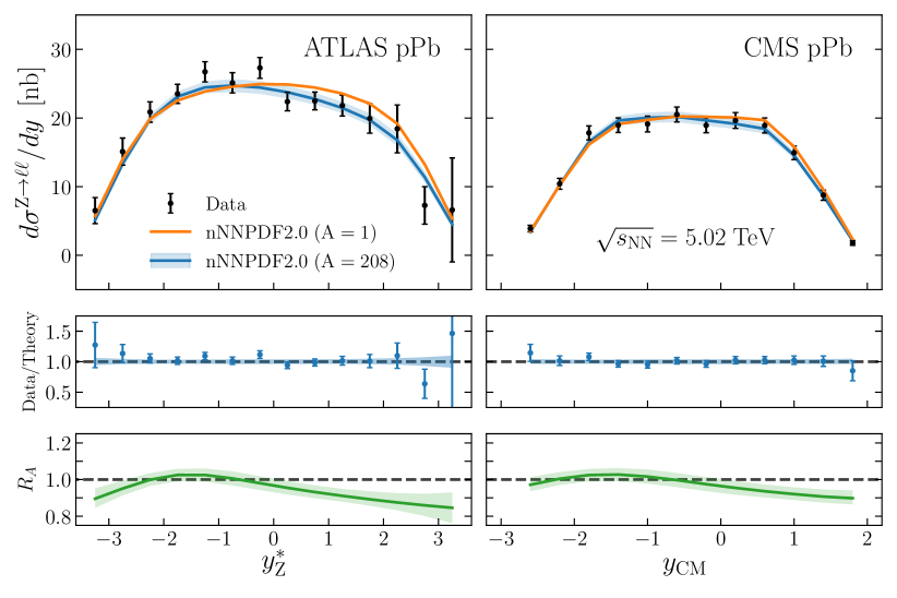
In Fig. 4.1 we display the comparison between the ATLAS and CMS measurements of Z boson production in proton-lead collisions at $\sqrt{s}=5.02$ TeV with the theoretical predictions using nNNPDF2.0. The theory calculations were computed using Eq. (4.1) with the nNNPDF2.0 $A=1$ and $A=208$ distributions, in the latter case also including the corresponding 90% CL uncertainty band. Note that for the theory cross-section obtained with the $A=1$ PDFs, nuclear effects are absent since it corresponds to the free proton distributions. From top to bottom, the three panels display the absolute cross-sections as a function of the dilepton rapidity $y$, the ratio between data and theory, and the nuclear modification factor ratio $R_{A}(y)$ defined by Eq. (4.2).

Here the ATLAS and CMS measurements of the dilepton rapidity distributions are both provided in the Z-boson center-of-mass reference frame. The CMS absolute cross-sections are lower than ATLAS due to the different kinematical selection cuts. We also note that for these datasets, as well as for the rest of LHC measurements, forward rapidities correspond to the direction of the incoming lead nuclei. From the comparisons in Fig. 4.1 we can see that the theory predictions are in good agreement with the experimental data. Interestingly, the $R_{A}(y)$ ratios exhibit a strong preference for nuclear modifications, especially at forward rapidities which correspond to small values in $x$ for the bound nucleons. As will be discussed below, this behavior can be explained at the level of the nuclear PDFs by a notable shadowing effect at small-$x$ for up and down quarks and antiquarks.

Figure 4.1: Comparison between the ATLAS (left) and CMS (right panel) measurements of Z boson production in proton-lead collisions at $\sqrt{s}=5.02$ TeV with the theoretical predictions using nNNPDF2.0 as input. We show the predictions obtained both for $A=1$ and $A=208$, in the later case including the 90% confidence level band. From top to bottom, the three panels display the absolute cross-sections, the ratio between data and theory, and the nuclear modification $R_{A}(y)$.

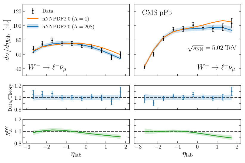
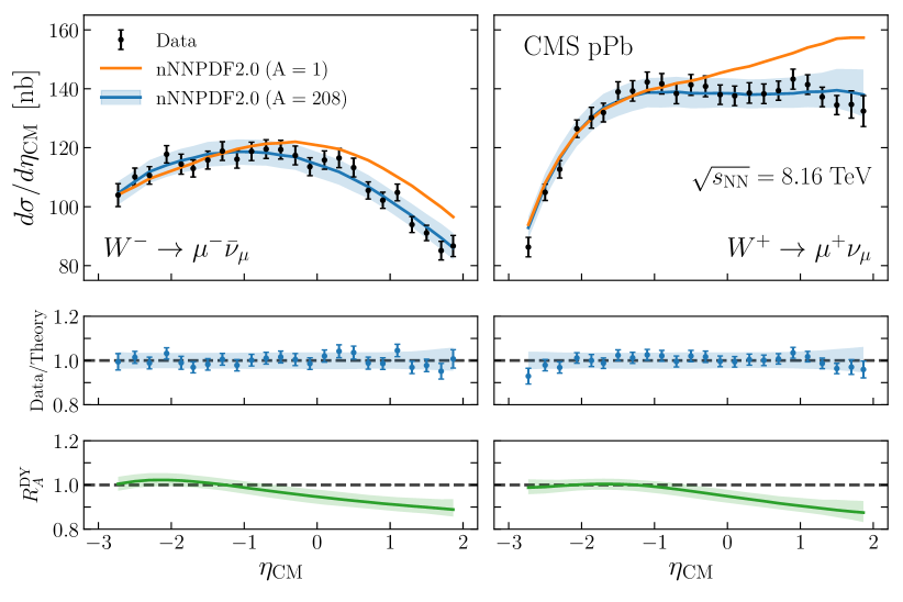
The corresponding comparisons for the CMS muon rapidity distributions in W^- and W⁺ production at $\sqrt{s}=5.02$ TeV and 8.16 TeV are displayed in Figs. 4.2 and 4.3 respectively. The results are presented as functions of the rapidity of the charged lepton from the W boson decay in the laboratory frame. In all cases the theoretical predictions based on nNNPDF2.0 provide a satisfactory description of the experimental data. It is interesting to note that for the high-statistics CMS measurement at 8 TeV, the $A=208$ prediction is remarkably better than the free-proton one, particularly at forward rapidities where one is sensitive to the small-$x$ region of the bound nucleons. This feature highlights how the CMS 8 TeV W production data provides direct evidence for the nuclear modifications of valence and sea quark distributions.

Figure 4.2: Same as Fig. 4.1 now for the CMS muon rapidity distributions in W^- and W⁺ production at $\sqrt{s}=5.02$ TeV.

Figure 4.3: Same as Fig. 4.1 now for the CMS muon rapidity distributions in W^- and W⁺ production at $\sqrt{s}=8.16$ TeV.

Nuclear parton distributions.

In Fig. 4.4 we display the nNNPDF2.0 set of nuclear PDFs for three different nuclei, ¹²C, ⁵⁶Fe, and ²⁰⁸Pb, constructed using Eq. (3.2) at a scale of $Q=10$ GeV. Specifically, we display the gluon, the up and down valence quarks, and the down, strange, and charm sea quark distributions. For isoscalar nuclei such as ¹²C, the up and down valence distributions are equivalent, $u_{v}^{(N/A)}=d_{v}^{(N/A)}$, as well as the up and down sea PDFs, $\bar{u}^{(N/A)}=\bar{d}^{(N/A)}$, as a result of Eq. (3.2).

Figure 4.4: The nNNPDF2.0 set of nuclear PDFs for ¹²C, ⁵⁶Fe, and ²⁰⁸Pb at the scale $Q=10$ GeV. We display the gluon, the up and down valence quarks (which coincide for isoscalar nuclei), as well as the down, strange, and charm sea quark distributions. The bands indicate the 90% CL uncertainty range.

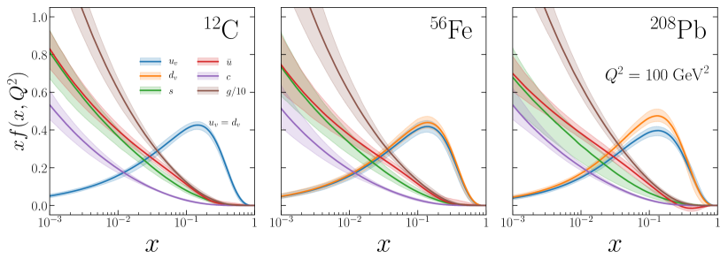
From the comparisons in Fig. 4.4, we can see that the nuclear PDFs exhibit a moderate dependence on the atomic number $A$. The resulting pattern of PDF uncertainties can partly be explained by the input data. For example, nPDF uncertainties on strangeness are smaller in ¹²C and ⁵⁶Fe compared to ²⁰⁸Pb, due to the impact of the proton boundary condition and the NuTeV dimuon data, respectively. We also observe that the PDF uncertainties on the gluon (and correspondingly on the dynamically generated charm PDF) at medium and small-$x$ are larger in iron than in carbon and lead. While the gluon uncertainties for carbon are largely determined by the impact of the free-proton boundary condition, those on lead nuclei can likely be attributed to the LHC measurements of W and Z production and the large amount of charged-current DIS data, which indirectly provide constraints via DGLAP evolution.

Fig. 4.4 also shows that in the case of ²⁰⁸Pb, there is a clear difference between the $d_{v}$ and $u_{v}$ distributions due to the isoscalar nature of the nucleus, where $d_{v}$ is larger due to the significant neutron excess in lead. The fact that $u_{v}$ and $d_{v}$ do not overlap within the 90% CL bands in a wide range of $x$ highlights how a careful treatment of the quark and antiquark flavor separation is essential in order to describe the precise data available on lead targets, especially the weak boson production measurements in proton-lead collisions at the LHC.

To further illustrate the features of the nNNPDF2.0 determination, it is useful to study them in terms of ratios with respect to the corresponding free-nucleon baseline. In the following we will define the nuclear modification ratios of PDFs for a nucleus with mass number $A$ as,

$$R_{f}^{A}(x,Q^{2})\equiv{{Zq^{(p/A)}_{f}(x,Q^{2})+(A-Z)q^{(n/A)}_{f}(x,Q^{2})}\over{Zq^{(p)}_{f}(x,Q^{2})+(A-Z)q^{(n)}_{f}(x,Q^{2})}}\,.$$ (4.4)

When evaluating Eq. (4.4), it is important to account both for the uncertainties associated to the nuclear and free-proton PDFs. In the case of a Monte Carlo set such as nNNPDF2.0, this entails evaluating $R_{f}^{A}$ for each of the $N_{\rm rep}$ replicas and then determining the resulting median and 90% CL interval.

Figure 4.5: Comparison of the nNNPDF2.0 parton distributions for $A=1$ with the NNPDF3.1 baseline used for the boundary condition in Eq. (3.17) at the parametrisation scale $Q_{0}=1$ GeV.

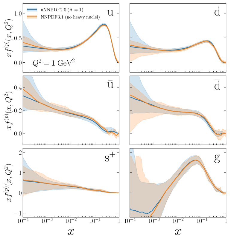
In Fig. 4.5 we show the nNNPDF2.0 distributions for $A=1$ that enter the denominator of Eq. (4.4). They are compared with the NNPDF3.1 proton baseline used for implementation the boundary condition via Eq. (3.17) at the input parametrisation scale $Q_{0}=1$ GeV. Overall, there is very good agreement between our $A=1$ result and the proton boundary condition, particularly in the region of $x$ where the constraint is being imposed, $10^{-3}<x<0.7$. It is important to emphasize that due to the nNNPDF2.0 $A=1$ set being determined not only by the boundary condition but also by the positivity constraints and the LHC cross-sections, one expects some moderate differences with the NNPDF3.1 proton baseline. The most notable differences indeed are found in the $\bar{u}$ and $\bar{d}$ PDFs at medium to large $x$, where the newly added DY positivity observables for $\bar{u}d$ and $u\bar{d}$ quark combinations, as well as the LHC proton-lead data, play a significant role. Nevertheless, the level of agreement reported in Fig. 4.5 is quite remarkable and highlights how the nNNPDF2.0 determination manages to take into account the extensive information provided by the global analysis of free-proton structure.

Figure 4.6: Comparison of the nuclear PDF ratios, Eq. (4.4), for three different nuclei, ¹²C, ⁵⁶Fe, and ²⁰⁸Pb, at $Q=10$ GeV. From top to bottom we show the up and down quarks, the corresponding antiquarks, the total strangeness, and the gluon. The bands indicate the 90% confidence level intervals and take into account the correlations with the proton baseline used for the normalisation.

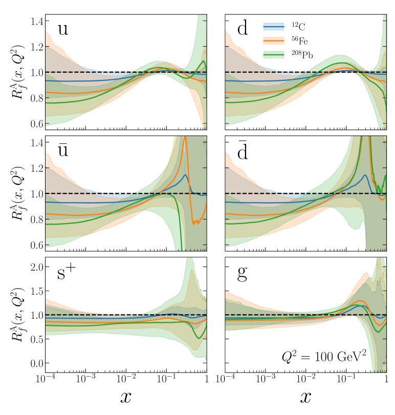
In Fig. 4.6 we display the nuclear PDF ratios, defined by Eq. (4.4), for the same parton flavors as in Fig. 4.5. Here the ratios for ¹²C, ⁵⁶Fe, and ²⁰⁸Pb nuclei are compared at $Q=10$ GeV. The shaded bands indicating the 90% confidence level intervals take into account also the correlations with the proton baseline. Overall, the comparison highlights the dependence on the central value and uncertainties of the nuclear ratios $R_{f}^{A}$ as the value of $A$ is varied from lighter to heavier nuclei.

For the up and down quark nPDFs in Fig. 4.6, we can see that the shadowing effects become more prominent at small-$x$ as $A$ increases, with the central value reaching $R_{f}^{A}\simeq 0.75$ at $x=10^{-4}$ for the lead ratios. Interestingly, the nPDF uncertainties on the quarks for $x\mathrel{\hbox to0.0pt{\lower 4.0pt\hbox{\hskip 1.0pt$\sim$}\hss}\raise 1.0pt\hbox{$<$}}10^{-2}$ are reduced in lead as compared to the lighter nuclei. This is a consequence of the constraints provided by the LHC data, as will be shown in Sect. 4.2. In the large-$x$ region, deviations from the $R_{f}^{A}=1$ scenario (no nuclear corrections) appear more prominent for the quarks and antiquarks of heavier nuclei.

Turning now to the valence quarks, one can distinguish the shadowing and anti-shadowing regions for all values of $A$, though nuclear effects in carbon are quite small. While one generally finds a suppression $R_{f}^{A}<1$ at large $x$ that is consistent with the EMC-effect expectation, the position of the so-called ”EMC minimum” is not universal or even guaranteed at the nPDF level. For the anti-quarks, the only region where a well-defined qualitative behavior is observed is the small-$x$ shadowing region, while at large-$x$ the nPDF uncertainties are too large to draw any solid conclusion. Finally, we observe that the nuclear modifications on the gluon nPDF are rather stable as $A$ is varied.

Comparison with EPPS16.

In Figs. 4.7 and 4.8, we display the nuclear PDF modification ratios at $Q=10$ GeV for iron, $R_{f}^{\rm Fe}(x,Q^{2})$, and lead, $R_{f}^{\rm Pb}(x,Q^{2})$, for nNNPDF2.0 and EPPS16, each normalized to the corresponding free-proton baseline. As in Fig. 4.6, we show the up and down quarks, the corresponding antiquarks, the total strangeness, and the gluon. The bands again correspond to the 90% CL uncertainties constructed using the appropriate prescription for each set. This means that for EPPS16, the error is computed by adding in quadrature the differences in value between the $N_{\rm eg}$ eigenvectors of the Hessian set and the best fit result.

Figure 4.7: The nuclear PDF modification ratios for iron, $R_{\rm Fe}(x,Q^{2})$, as a function of $x$ for $Q=10$ GeV for both nNNPDF2.0 and EPPS16. From top to bottom we show the up and down quarks, the corresponding antiquarks, the total strangeness, and the gluon. The bands correspond to the 90% CL uncertainties, and each nPDF set is normalised to its corresponding free-proton baseline as indicated by Eq. (4.4).

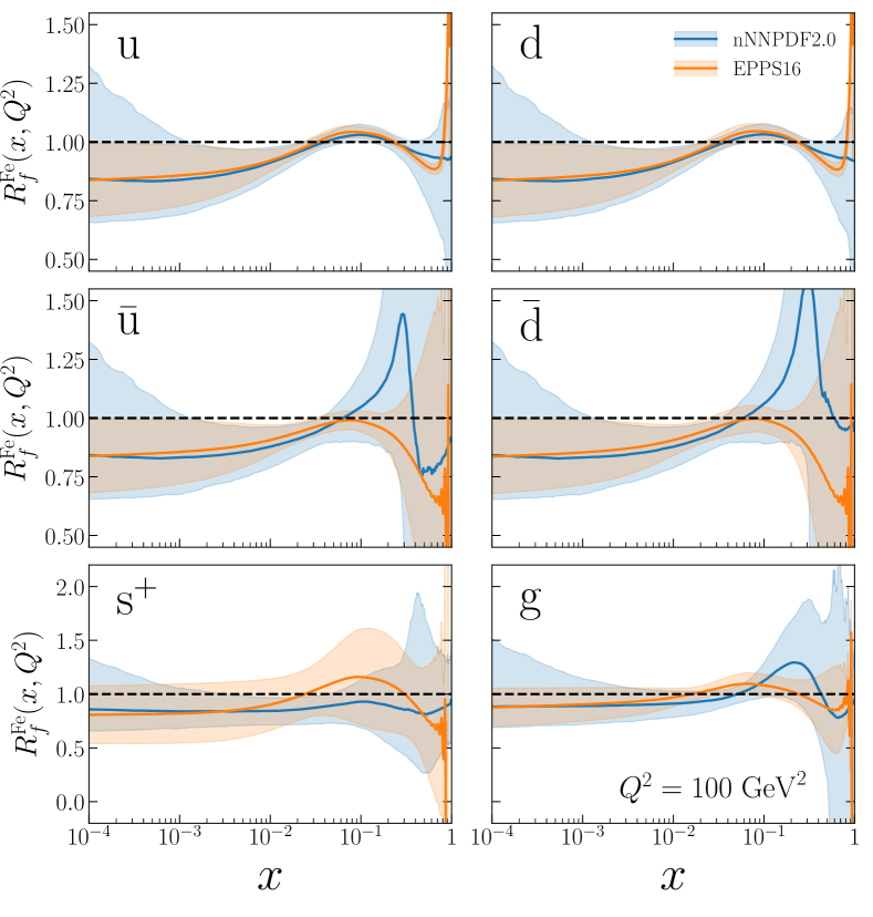
Beginning with the nPDF comparison for iron nuclei, we find that there is good agreement between the results of nNNPDF2.0 and EPPS16 both in terms of central values and of the nPDF uncertainties in the range of $x$ for which experimental data is available. In the small- and large-$x$ extrapolation regions, the uncertainties are larger in the nNNPDF2.0 case. We also note that the Fermi-motion-like growth of $R_{u}^{\rm Fe}$ and $R_{d}^{\rm Fe}$ at very large $x$, which is built into the EPPS16 parameterization, is absent in the nNNPDF2.0 results. There instead one finds a suppression compared to the free-proton case, especially in the case of $R_{d}^{\rm Fe}$. As expected, the observed pattern of nuclear modifications is very similar between up and down quarks and between the corresponding antiquarks due to iron being nearly isoscalar.

Considering the behavior of the sea quarks, nNNPDF2.0 and EPPS16 agree well in terms of central values and uncertainties in the shadowing region, $x\mathrel{\hbox to0.0pt{\lower 4.0pt\hbox{\hskip 1.0pt$\sim$}\hss}\raise 1.0pt\hbox{$<$}}0.05$. However, there are more significant differences at large-$x$, where the qualitative behavior between the two nPDF sets is the opposite: nNNPDF2.0 favors an enhancement compared to the free-proton baseline, while EPPS16 prefers instead a suppression. In any case, the differences are well within the large uncertainty bands, and additional data is needed to be able to ascertain the correct behavior in this region. Note that at large-$x$ the free-proton baseline antiquarks are also affected by large errors, complicating the interpretation of $R_{\bar{u}}^{\rm Fe}$ and $R_{\bar{d}}^{\rm Fe}$.

Turning to the nuclear modification of the total strangeness, in nNNPDF2.0 we find a suppression of $\sim 20$% compared to the proton baseline in the relevant range of $x$. This is consistent with studies of the interplay between the NuTeV dimuon and the ATLAS W,Z 2011 data in proton global analyses, where the latter data set largely suppress strangeness in contrast to the former. Such behavior is not reported by EPPS16, which exhibits much larger nPDF uncertainties that are likely due to the absence of the strange-sensitive NuTeV cross-sections in their analysis. Furthermore, the ATLAS W,Z 2011 distributions are missing from the CT14 proton baseline used by EPPS16 (although these data have been accounted for in the recent CT18 release Hou:2019efy ).

Figure 4.8: Same as Fig. 4.7 in the case of lead nuclei, $R_{\rm Pb}(x,Q^{2})$.

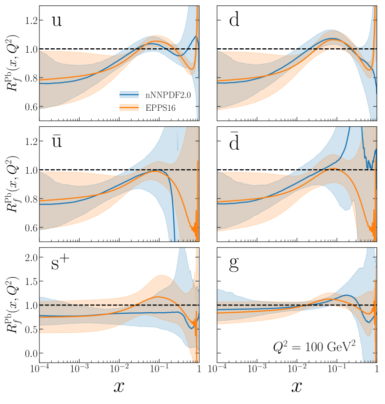
Finally, concerning the gluon PDF we find from this comparison that in the nNNPDF2.0 fit there is little evidence for nuclear shadowing, with $R_{g}^{\rm Fe}\simeq 1$ in the region $x\leq 0.05$. We also find that the nPDF uncertainties on the gluon are larger compared to EPPS16 by roughly a factor of two. At larger values of $x$, the uncertainties increase significantly and nNNPDF2.0 prefers a suppressed central value, unlike EPPS16. We note that neither of the two analyses include direct constraints on the large-$x$ nuclear gluons, hence the sizeable nPDF uncertainties, although available data on dijet and photon production could improve this situation.

In the corresponding comparison for lead nuclei, displayed in Fig. 4.8, one observes a number of similarities and differences with respect to the nPDFs of iron. Concerning the up and down quarks, we find our nNNPDF2.0 result provides significant evidence for shadowing at small-$x$. For instance, at $x\simeq 5\times 10^{-3}$ we obtain $R_{u}^{\rm Pb}\neq 1$ at the four-sigma level or higher. Interestingly, nPDF uncertainties in the shadowing region are up to a factor of two smaller in nNNPDF2.0 than in EPPS16. While in both cases anti-shadowing at $x\simeq 0.1$ is observed, the larger $x$ qualitative behavior is different between the two analyses, with EPPS16 finding the (built-in) EMC suppression followed by Fermi-motion rise while in nNNPDF2.0 the pattern of nuclear modifications is different. In any case, the agreement between the central values of nNNPDF2.0 and EPPS16 for $R_{u}^{\rm Pb}$ and $R_{d}^{\rm Pb}$ in the region of $x\mathrel{\hbox to0.0pt{\lower 4.0pt\hbox{\hskip 1.0pt$\sim$}\hss}\raise 1.0pt\hbox{$<$}}0.3$ is quite remarkable given the very different methodologies employed in each study.

Concerning the nuclear modifications of the sea quarks in lead nuclei, one finds a similar qualitative behavior as in the case of iron. For $x\mathrel{\hbox to0.0pt{\lower 4.0pt\hbox{\hskip 1.0pt$\sim$}\hss}\raise 1.0pt\hbox{$<$}}0.1$ there is good agreement between the central values of $R_{\bar{u}}^{\rm Pb}$ and $R_{\bar{d}}^{\rm Pb}$ between EPPS16 and nNNPDF2.0, with the latter exhibiting smaller uncertainties. The two sets are more notably different for $x\mathrel{\hbox to0.0pt{\lower 4.0pt\hbox{\hskip 1.0pt$\sim$}\hss}\raise 1.0pt\hbox{$>$}}0.1$ instead, where EPPS16 predicts a EMC-like suppression common to $\bar{u}$ and $\bar{d}$ while nNNPDF2.0 favours a large suppression for $\bar{u}$ but an enhancement for $\bar{d}$. However, the large nPDF uncertainties in this region prevent any definitive conclusions, though the two fits are fully consistent within the 90% CL bands. One possible source for the differences could be in the respective free-proton counterparts, where large-$x$ antiquarks are poorly known. For the total strangeness, the behavior of $R_{s^{+}}^{\rm Pb}$ is similar to that of iron, where nNNPDF2.0 predicts a suppression more or less independent of $x$, with rather larger uncertainties for EPPS16 compared to our nNNPDF2.0 result due to the missing constraints from the NuTeV dimuon cross-sections.

Finally, regarding the nuclear modifications of the lead gluon PDF illustrated in the bottom right panel of Fig. 4.8, we again find that $R_{g}^{\rm Pb}$ agrees with unity across all relevant $x$. Here the initial-scale differences are washed out partially by DGLAP evolution, but clearly the shadowing in the nuclear gluons is less apparent than for the quarks. Although the nPDF uncertainties increase at large $x$ due to the lack of direct constraints, the qualitative behavior of $R_{g}^{\rm Pb}$ differs between the two PDF determinations.

Nuclear strangeness.

The strangeness content of the proton in unpolarized PDF fits has attracted a lot of attention recently. Traditionally, the determination of $s(x,Q^{2})$ in global proton PDF fits has been dominated by the constraints provided by charm production in neutrino DIS Bazarko:1994tt ; chorus-dimuon ; MasonPhD ; Mason:2007zz ; Samoylov:2013xoa . These measurements suggest that the strange sea is suppressed compared to its up and down quark counterparts, favoring values of around $r_{s}\simeq 0.5$ when expressed in terms of the strangeness ratio defined as

$$r_{s}(x,Q^{2})\equiv{{s(x,Q^{2})+\bar{s}(x,Q^{2})}\over{\bar{u}(x,Q^{2})+\bar{d}(x,Q^{2})}}\,.$$ (4.5)

Other strange-sensitive processes agree qualitatively with the constraints on $r_{s}$ provided by the neutrino DIS data, such as W production in association with charm quarks Stirling:2012vh from CMS Chatrchyan:2013uja ; CMS-PAS-SMP-18-013 ; Sirunyan:2018hde and ATLAS 7 TeV Aad:2014xca , and semi-inclusive deep-inelastic scattering (SIDIS) Airapetian:2013zaw ; Borsa:2017vwy ; Sato:2019yez . However, the ATLAS measurements of the leptonic rapidity distributions in inclusive W and Z production at 7 TeV Aad:2012sb ; Aaboud:2016btc exhibit instead a strong preference for a symmetric strange sea with $r_{s}\simeq 1$. One should point out that general considerations based on perturbative DGLAP evolution imply that $r_{s}\to 1$ at large $Q$ and small-$x$, but at low $Q$ and medium/large-$x$ the value of $r_{s}$ is dictated by non-perturbative dynamics.

As was motivated in Ref. Ball:2018twp , it is important to carefully assess the nuclear uncertainties associated to the nuclear strangeness, given that these will potentially affect the determination of the proton strangeness from global fits based on neutrino data. We display in Fig. 4.9 the strangeness ratio $r_{s}(x,Q^{2})$ defined by Eq. (4.5) obtained with our nNNPDF2.0 result for ¹p, ⁵⁶Fe, and ²⁰⁸Pb at both the input parameterization scale $Q_{0}=1$ GeV and at a higher scale of $Q=10$ GeV.

Figure 4.9: The strangeness ratio $r_{s}(x,Q^{2})$, defined in Eq. (4.5), in nNNPDF2.0 comparing the results for the free-proton baseline, ⁵⁶Fe, and ²⁰⁸Pb at both the input parametrisation scale $Q_{0}=1$ GeV (left) and at a higher scale $Q=10$ GeV (right plot).

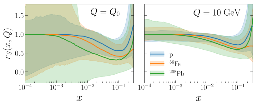
From the comparison in Fig. 4.9 we find that at the input parameterization scale $r_{s}$ is particularly suppressed in the case of lead, where the central value of nNNPDF2.0 satisfies $r_{s}<0.5$ for $5\cdot 10^{-3}\mathrel{\hbox to0.0pt{\lower 4.0pt\hbox{\hskip 1.0pt$\sim$}\hss}\raise 1.0pt\hbox{$<$}}x\mathrel{\hbox to0.0pt{\lower 4.0pt\hbox{\hskip 1.0pt$\sim$}\hss}\raise 1.0pt\hbox{$<$}}0.2$. A similar preference for a suppressed strange sea, albeit less pronounced, can be seen in iron nuclei. In any case, the nPDF uncertainties affecting this ratio are rather large, in particular for the heavier nuclei. The fact that for $x\mathrel{\hbox to0.0pt{\lower 4.0pt\hbox{\hskip 1.0pt$\sim$}\hss}\raise 1.0pt\hbox{$<$}}10^{-3}$ one obtains $r_{s}\simeq 1$ for all three nuclei is a consequence of the parameterization preprocessing, whose ranges are chosen to ensure that in the small-$x$ extrapolation region all quark and antiquark flavors behave in the same way (see Figs. 3.2 and 3.1). Once DGLAP evolution takes place, $r_{s}$ tends to become closer to unity across a wider range in $x$, but even at the higher scale a suppressed strangeness for $x\mathrel{\hbox to0.0pt{\lower 4.0pt\hbox{\hskip 1.0pt$\sim$}\hss}\raise 1.0pt\hbox{$>$}}0.01$ is preferred for both iron and lead.

The results in Fig. 4.9 suggest that including neutrino CC structure functions such as CHORUS and NuTeV in proton PDF fits without accounting for nuclear uncertainties might not be a justified approximation, given the current precision that modern fits achieve. It will be interesting nonetheless to determine the impact on the global NNPDF proton PDF fits when nNNPDF2.0 is used to account for nuclear uncertainties using the procedure outlined in Ref. Ball:2018twp .

4.2 Comparison with nNNPDF1.0

We now turn to study the differences between the nNNPDF1.0 and nNNPDF2.0 determinations by tracing back the impact of the various improvements in the latter with a series of comparisons. The goal of this exercise is to assess which of these differences can be identified with specific methodological improvements, such as the cross-section positivity constraint, and which ones are related to the impact of the new experimental information, either the DIS charged current structure functions or the LHC gauge boson production measurements.

The starting point for this study will be a fit denoted nNNPDF1.0r, which has been obtained with the code used to produce nNNPDF2.0 but using the same theory, methodology settings, and input dataset as in the nNNPDF1.0 analysis. The only differences at this level are related to optimizations and improvements implemented in the code to speed up its performance. We have verified that nNNPDF1.0 and nNNPDF1.0r are statistically indistinguishable, thus we can safely adopt the latter as baseline for the comparisons in what follows.

We have then produced several variants of this nNNPDF1.0r baseline, each time adding one extra feature or dataset. The first of these two variants is a fit where the proton boundary condition has been updated to the no-nuclear NNPDF3.1 fit shown in Fig. 3.3. The second is a fit where, in addition to the updated boundary condition, the positivity of cross-sections has been imposed following the procedure described in Sect. 3.3. We display in Fig. 4.10 the comparison between nNNPDF1.0r and these two fit variants. Since the isoscalar neutral-current DIS structure functions used in nNNPDF1.0 are primarily sensitive to the specific quark combination $\Sigma+T_{8}/4$, we plot this together with the gluon distribution as a function of $x$ at $Q^{2}=10$ GeV² for carbon, iron, and lead.

Figure 4.10: Comparison between the nNNPDF1.0r baseline and two fit variants based on the same input dataset, one where the proton boundary condition has been updated and another where in addition the positivity of physical cross-sections has been imposed. We show the $\Sigma+T_{8}/4$ quark combination (left) and gluon (right) at $Q^{2}=10$ GeV² for three values of $A$.

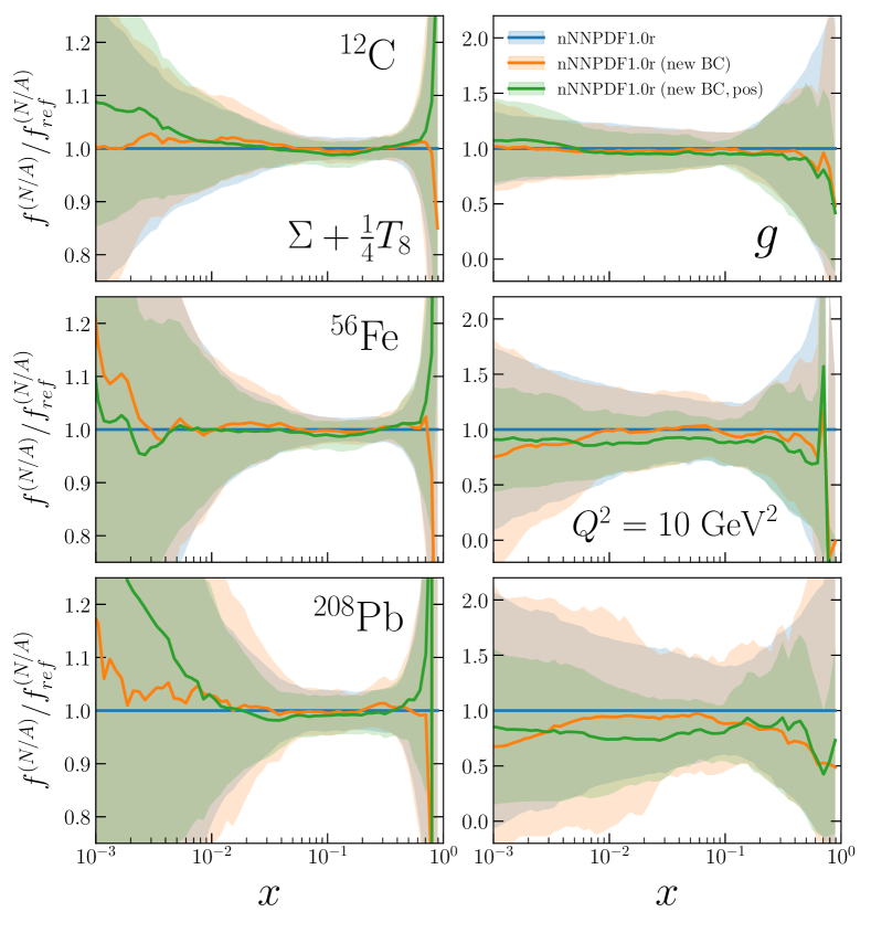
First, one can see from Fig. 4.10 that the impact of the new proton boundary condition in the nuclear fit is generally moderate concerning the size of the uncertainty band. There are some differences at the central value level for the small-$x$ quarks and for the nuclear gluon PDF of lead, but in both cases the shifts are much smaller than the associated uncertainties. This does not imply that using the updated proton boundary condition is irrelevant for nNNPDF2.0, but rather that this choice is not particularly impactful for the specific PDF combinations that can be constrained by the nNNPDF1.0 dataset. As shown in Fig. 3.3, the differences between the two variants of the proton boundary conditions are more distinguished for the total strangeness compared to the other quark flavors.

On the other hand, imposing the positivity of the cross-sections leads to more important differences. This is not completely unexpected, since it is well known that in general a model-independent (n)PDF analysis will lead to some cross-sections being negative unless their positivity is explicitly imposed. In our case, one finds that there is not much difference in the quarks, but there are clear changes for the nuclear gluons in iron and lead, especially in the latter. Here we see that imposing the positivity of cross-sections leads to a significant reduction of the nPDF uncertainty band, which in the case of lead can be up to a factor of two.

Figure 4.11: The longitudinal structure function $F_{L}(x,Q^{2})$ at the positivity scale $Q^{2}=5$ GeV. We compare the predictions of the nNNPDF1.0r(newBC) fits with and without the cross-section positivity constraint imposed. We show the extrapolation (left) and the data (right) regions, in the former case displaying also the predictions from the individual replicas in the nNNPDF1.0r(newBC) fit that do not satisfy the positivity constraints.

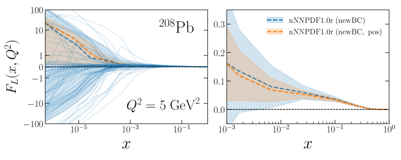
To illustrate the impact of the cross-section positivity constraint, we display in Fig. 4.11 the longitudinal structure function $F_{L}(x,Q^{2})$ at the positivity scale $Q^{2}=5$ GeV. We compare the predictions of the nNNPDF1.0r fits including the updated proton boundary condition with and without the cross-section positivity constraint imposed in both the extrapolation and the data regions. In the left panel, we display also the predictions from the individual replicas of the nNNPDF1.0r(newBC) fit that do not satisfy the cross-section positivity constraints. Indeed, one can observe that many $F_{L}$ replicas become negative in some region of $x$ unless this constraint is explicitly imposed, and that removing them leads to a significant reduction of the nPDF uncertainties, particularly in the small-$x$ region. Interestingly, at medium-$x$ it is largely the upper (rather than the lower) 90% CL limit which is reduced by the positivity constraint: this can be explained by the fact that the very negative $F_{L}$ replicas at small-$x$ were actually higher than the median value at medium-$x$ in order to satisfy the momentum sum rule.

Figure 4.12: Same as Fig. 4.8 now comparing the nNNPDF2.0 baseline results with those of a fit based on identical settings but restricted to a DIS-only dataset.

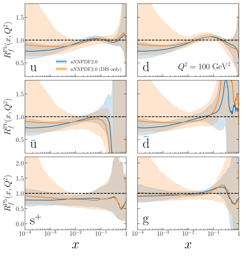
Concerning the impact of the new datasets, a direct comparison of the nNNPDF1.0r-like fits with those including CC DIS and LHC data is not possible since as discussed in Sect. 3.2 the input parameterization basis and the flavor assumptions are different. However, we are still able to assess the relative contribution of the CC structure functions and the LHC gauge boson cross-sections in determining the nNNPDF2.0 results. In Fig. 4.12 we display the nuclear modification ratios for the nPDFs in lead, as was shown in Fig. 4.8, but now comparing the nNNPDF2.0 baseline results with those of a fit that is restricted to DIS structure functions, including charged-current scattering, and that uses identical theoretical and methodological settings.

One of the most remarkable features of this comparison is the sizeable impact that LHC measurements have in reducing the uncertainties of the nuclear PDFs. This effect is particularly significant for the gluon and for all quark flavors at $x\mathrel{\hbox to0.0pt{\lower 4.0pt\hbox{\hskip 1.0pt$\sim$}\hss}\raise 1.0pt\hbox{$<$}}0.1$. On one hand, the LHC data clearly reveals the presence of nuclear shadowing at small-$x$ for both the valence and sea quarks, something which is not accessible in a DIS-only fit. This result is consistent with the nuclear modification ratios for the LHC Drell-Yan distributions reported e.g. in Fig. 4.3. On the other hand, the impact of the LHC data on the central values and uncertainties of nNNPDF2.0 at $x\mathrel{\hbox to0.0pt{\lower 4.0pt\hbox{\hskip 1.0pt$\sim$}\hss}\raise 1.0pt\hbox{$>$}}0.1$ is less prominent, although in that region one also observes a reduction of the uncertainties. The fact that $R_{\bar{u}}\ll 1$ and $R_{\bar{d}}\gg 1$ for lead nuclei at large-$x$ is already present at the level of DIS-only fits implies that this trend is favored by the CHORUS and NuTeV charged-current structure functions.

4.3 The momentum and valence integrals in nuclei

As was discussed in Sect. 3.2, we impose three sum rules in the nNNPDF2.0 determination, namely the momentum sum rule, Eq. (3.7), and the two valence sum rules, Eqns. (3.2) and (3.2). These constraints are satisfied by adjusting the overall prefactors $B_{f}$ in Eq. (3.6) for the gluon $g$, the total valence $V$, and the valence triplet $V_{3}$ distributions, respectively. Furthermore, they are independently imposed for each value of $A$ for which there is available experimental data.

Here we investigate the role played by these sum rules in the global nPDF determination. In particular, we address whether or not the physical requirements of energy and valence quark number conservation are satisfied by the phenomenological fit to experimental data (within uncertainties) when the sum rules are not explicitly imposed. Recently, theoretical arguments have been put forward that the momentum sum rule for nucleons in nuclei might not hold Brodsky:2019jla . Motivated in this respect, we have carried out a similar study to the one presented in Ref. Ball:2011uy , where global proton PDF fits without imposing the momentum sum rule were performed. In the proton case, while the LO prediction for the momentum integral was to be far from the QCD expectation, both the NLO and NNLO fits exhibited remarkable agreement at the $\simeq 1\%$ level Ball:2011uy .

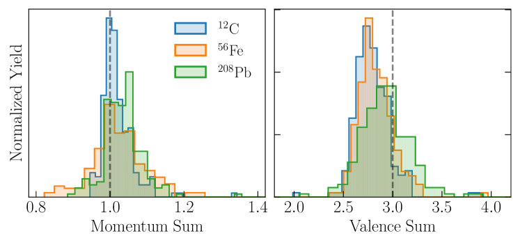
We have therefore produced two variants of the nNNPDF2.0 analysis, each based on $N_{\rm rep}=250$ replicas, where either the momentum sum rule or the total valence sum rule is not imposed. Afterwards, we evaluate in each case the corresponding momentum and total valence integrals, defined as

$$I_{\rm M}(A)\equiv\int_{0}^{1}dx\,x\left(\Sigma^{(p/A)}(x,Q_{0})+g^{(p/A)}(x,Q_{0})\right)\,,$$ (4.6)

$$I_{\rm V}(A)\equiv\int_{0}^{1}dx\leavevmode\nobreak\ V^{(p/A)}(x,Q_{0})\,,$$ (4.7)

and assess whether or not they are in agreement with the QCD expectations, namely $I_{\rm M}(A)=1$ and $I_{V}(A)=3$ respectively. One should note that the momentum and valence sum rules are already satisfied at the level of the proton boundary condition, and thus some constraints are expected to be propagated to the lighter nuclei. However, the analysis of Ref. Ball:2011uy demonstrates that results would be largely unchanged if the momentum and valence sum rules would have been excluded also from the free-proton baseline.

In Fig. 4.13 we display the distribution of the momentum and valence integrals, Eqns. (4.6) and (4.7), respectively, in the variants of the nNNPDF2.0 fit where the corresponding sum rules are not being explicitly imposed. We show the relative frequency of the momentum and valence integral for three representative nuclei: ¹²C, ⁵⁶Fe, and ²⁰⁸Pb. The dashed vertical line in Fig. 4.13 indicates the QCD expectations for $I_{\rm M}(A)$ and $I_{\rm V}(A)$. The corresponding values for the 90% confidence level intervals for each of these two integrals for the relevant values of $A$, as well as for the free-proton baseline $A=1$, can be found in Table 4.3.

Figure 4.13: The distribution of the momentum (left) and total valence (right panel) integrals, Eqns. (4.6) and (4.7) respectively, in the variants of the nNNPDF2.0 determination where the corresponding sum rules have not been explicitly imposed. We show the relative frequency of the momentum and valence integral for three representative nuclei: ¹²C, ⁵⁶Fe, and ²⁰⁸Pb. The dashed vertical line indicates the corresponding the QCD expectations, $I_{\rm M}(A)=1$ and $I_{\rm V}(A)=3$. The associated 90% CL ranges are reported in Table 4.3.

$\qquad\qquad A\qquad\qquad$	$\qquad\qquad I_{\rm M}(A)\qquad\qquad$	$\qquad\qquad I_{\rm V}(A)\qquad\qquad$
1	$\left[0.99,1.06\right]$	$\left[2.53,3.12\right]$
12	$\left[0.97,1.10\right]$	$\left[2.56,3.11\right]$
56	$\left[0.90,1.16\right]$	$\left[2.58,3.16\right]$
208	$\left[0.94,1.12\right]$	$\left[2.54,3.34\right]$

Table 4.3: The 90% CL ranges for the momentum and valence integrals, Eqns. (4.6) and (4.7), in the variants of the nNNPDF2.0 fits whether either one or the other sum rule is not imposed.

From the results presented in Fig. 4.13 and Table 4.3 one finds that the momentum integral is in agreement with the QCD expectation, $I_{\rm M}(A)=1$, within uncertainties for all nuclei. In the case of ¹²C for example, one finds that $0.97\mathrel{\hbox to0.0pt{\lower 4.0pt\hbox{\hskip 1.0pt$\sim$}\hss}\raise 1.0pt\hbox{$<$}}I_{\rm M}\mathrel{\hbox to0.0pt{\lower 4.0pt\hbox{\hskip 1.0pt$\sim$}\hss}\raise 1.0pt\hbox{$<$}}1.10$ at the 90% confidence level, with somewhat larger uncertainties for the heavier nuclei. Even for lead, where the proton boundary condition has little effect, the median of the distribution is reasonably close to the QCD expectation. The uncertainties on $I_{\rm M}$ are larger in the nuclear PDF analysis than the $\simeq 1\%$ error found in the proton case Ball:2011uy , as expected since the experimental data for nuclear collisions is far less abundant and further distributed between different nuclei. Nevertheless, the overall consistency with the QCD expectations is quite compelling. Note also that here the proton boundary condition is imposed only for $x\geq 10^{-3}$, and therefore our prediction for $I_{\rm M}(A=1)$ is expected be less accurate as compared to the proton global analysis case.

The result that the momentum integral agrees with the theoretical predictions for all nuclei is a non-trivial validation of the global nuclear PDF analysis framework based on the QCD factorization hypothesis. It further demonstrates the robustness of our fitting methodology, in that the resulting nPDFs are reasonably stable regardless of whether or not the momentum sum rule is imposed during the fit. To illustrate better this latter point, in Fig. 4.14 we provide a comparison between the baseline nNNPDF2.0 fit at $Q_{0}=1$ GeV with the variant in which the momentum sum rule is not being imposed. We show the total quark singlet and the gluon for both ⁵⁶Fe and ²⁰⁸Pb. Recall that the momentum sum rule is used to fix the overall gluon normalization in Eq. (3.6). In the case of lead, where the experimental constraints are relatively abundant, we find that both the singlet and the gluon are reasonably similar irrespective of whether or not the momentum sum rule is imposed. The momentum sum rule plays a larger role in iron, especially in reducing the gluon nPDF uncertainties, but interestingly the central value of the all distributions is quite stable when comparing the two fits. This stability is consistent with the results reported in Fig. 4.13.

Figure 4.14: Comparison of the baseline nNNPDF2.0 fit at $Q_{0}=1$ GeV with the variant in which the momentum sum rule is not being imposed. We show the total quark singlet (left) and the gluon (right) for ⁵⁶Fe (upper) and ²⁰⁸Pb (lower panels).

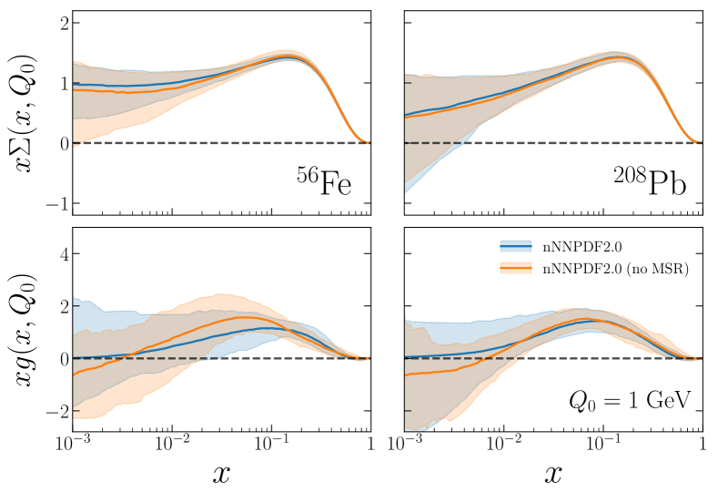
The main conclusions are qualitatively similar for a fit in which the total valence sum rule has not been imposed. Results of this fit are displayed in the right panel of Fig. 4.13, where the normalized frequency of the total valence integral are shown for the same three nuclei discussed previously. The corresponding 90% CL intervals are also reported in Table 4.3. Similar to the momentum sum results, we find that for the valence integral the fit results agree with the QCD expectations within uncertainties. The preferred value of the valence integral (median) turns out to be $I_{\rm V}\simeq 2.8$ irrespective of $A$. This implies that even when Eq. (4.7) is not imposed explicitly, the experimental measurements favor the QCD prediction within 5% for all values of $A$ relevant for the present study. We have also verified that, in a similar way as in Fig. 4.14, the resulting nPDFs are reasonably stable regardless of whether or not the valence sum rule is imposed.

Putting together the results of these two exercises, one can conclude that the fit results are relatively stable in the nNNPDF framework even in the absence of the sum rules, consistent with the fact that experimental data and the QCD expectations based on the factorization theorem are in agreement with each other for hard-scattering collisions involving heavy nuclei.

4.4 The positivity of physical cross-sections

As was discussed in Sect. 3.3, we impose the requirement that the cross-sections of arbitrary physical processes are positive-definite quantities. This constraint is implemented by means of an additive penalty term in the figure of merit, Eq. (3.18). Moreover, the penalty is constructed from the pseudo-data summarized in Table 3.1, which corresponds to lepton-nuclear scattering structure functions and Drell-Yan cross-sections in proton-nucleus collisions. Recall that the kinematics of the positivity pseudo-data were chosen to cover those of the actual data used in the fit, see Fig. 2.1.

Here we want to demonstrate that the nNNPDF2.0 determination indeed satisfies these various positivity constraints. In Fig. 4.15 we display a representative selection of the positivity observables imposed in nNNPDF2.0. In particular, we show the DIS structure functions $F_{2}^{s}(x,Q^{2})$ and $F_{L}(x,Q^{2})$, as well as the Drell-Yan rapidity distributions $\sigma_{u\bar{u}}^{\rm DY}(y)$ and $\sigma_{\bar{u}d}^{\rm DY}(y)$, where the bands indicates the 90% confidence level uncertainty interval. We use a scale of $Q^{2}=5$ GeV², which corresponds to the same scale in which Eq. (3.18) is imposed. Furthermore, we provide the positivity predictions for both iron and lead nuclei. Note that since the Drell-Yan cross-sections are not normalized by the value of $A$, the absolute magnitude of the two nuclei are different. Of course, the overall normalization is not relevant for the implementation of the positivity constraint.

Figure 4.15: A representative selection of the positivity observables used in nNNPDF2.0. From top to bottom and from left to right, we show the DIS structure functions $F_{2}^{s}$ and $F_{L}$ and the Drell-Yan rapidity distributions $\sigma_{u\bar{u}}^{\rm DY}$ and $\sigma_{\bar{u}d}^{\rm DY}$. The bands indicate the 90% confidence level interval.

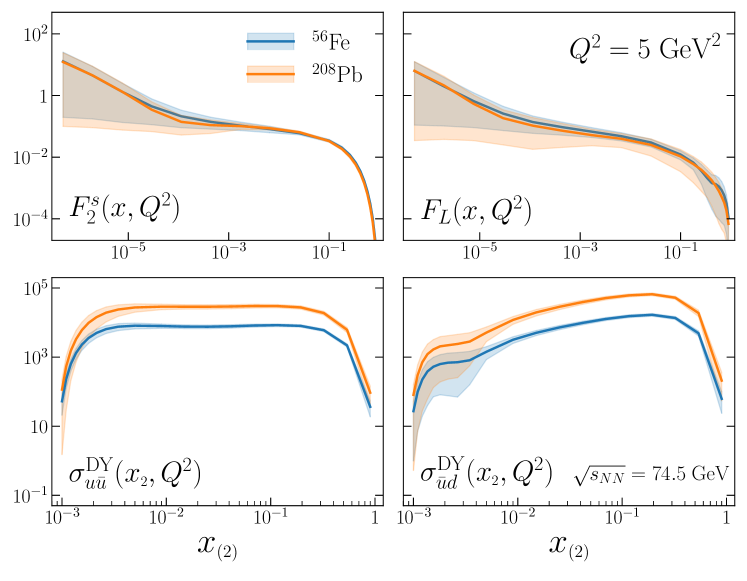
The selection of positivity observables in Fig. 4.15 is representative since it contains one of the quark structure functions ($F_{2}^{s}$) constraining a $q^{+}$ combination, $F_{L}$ that is sensitive to the gluon positivity, and a diagonal and off-diagonal DY cross-section which are relevant for different aspects of quark flavor separation (confer also the LO expressions in App. A). Here the Drell-Yan cross-sections are represented as a function of $x_{2}$, which corresponds to the momentum fraction of the nuclear projectile obtained using the LO kinematics of Eq. (A.15). While the positivity constraint was only implemented for $x_{2}\mathrel{\hbox to0.0pt{\lower 4.0pt\hbox{\hskip 1.0pt$\sim$}\hss}\raise 1.0pt\hbox{$>$}}10^{-2}$ with a per-nucleon center-of-mass energy of $\sqrt{s}=23.5$ GeV, we illustrate instead the positivity for a choice of kinematics that allow a reach to $x_{2}\sim 10^{-3}$, with a per-nucleon center-of-mass energy of $\sqrt{s}=74.5$ GeV. As can be seen from Fig. 4.15, the nNNPDF2.0 determination satisfies the positivity of physical cross-sections in the entire kinematic range. Here the nPDF uncertainty bands become larger near the kinematic endpoints ($x=1$ for DIS and $x_{2}\simeq 10^{-3}$ for Drell-Yan), since these correspond to regions of the phase space where experimental constraints are scarce. Recall that by virtue of DGLAP evolution properties, these results ensure the cross-sections involving higher momentum transfers, $Q^{2}>5$ GeV², will also be positive provided one maintains the initial coverage in $x_{2}$. Therefore, we conclude that while we have not explicitly imposed the positivity at the level of the nuclear PDFs, physical observables constructed from nNNPDF2.0 are guaranteed to satisfy the positivity requirement.

5 Implications for photon and hadron production in nuclear collisions

In this section we discuss some phenomenological applications of the nNNPDF2.0 determination. Theoretical predictions for isolated photon production in proton-lead collisions at the LHC are first compared with recent measurements from the ATLAS collaboration taken at $\sqrt{s}=8.16$ TeV. We then revisit the potential of the FoCal upgrade to the ALICE detector in constraining the small-$x$ gluon nuclear PDF using measurements of direct photon production in the forward region. Finally, we provide predictions based on nNNPDF2.0 for inclusive hadron production in proton-nuclear collisions, a process that can constrain both the quark and gluon nuclear PDFs as well as the corresponding fragmentation functions in vacuum and in medium.

Several additional applications of our nNNPDF2.0 result are expected to be of phenomenological interest. In particular, our nPDFs could be used to study the constraining power of inclusive and heavy quark structure function measurements at the recently approved Electron Ion Collider (EIC) Boer:2011fh and the proposed Large Hadron electron Collider (LHeC) AbelleiraFernandez:2012cc . Initial studies based on nNNPDF1.0 and EIC neutral-current structure function pseudo-data were presented in Ref. AbdulKhalek:2019mzd . However, updated projections for EIC pseudo-data are now being finalized based on more realistic accelerator and detector settings. We will therefore defer an update to our nNNPDF1.0 study of EIC pseudo-data to an upcoming Conceptual Design Report where the more accurate EIC specifications will be presented together with impact studies from various nuclear PDF analysis groups.

5.1 Isolated photon production in pA collisions with ATLAS

Production of isolated photons in proton-proton collisions is primarily sensitive to the gluon content of the proton via the QCD Compton scattering process Vogelsang:1995bg ; Ichou:2010wc . However, several complications associated with the measurement of photon production complicate a clean interpretation in terms of hard-scattering cross-sections, such as the need for subtracting the fragmentation component and the removal of photons coming from pion decays. Although early PDF fits used photon production in fixed-target scattering to constrain the gluon data, the data were eventually discarded in favor of the cleaner and more abundant data on jet production at the TeVatron Gao:2017yyd . However, photon production measurements from ATLAS and CMS were later revisited using NLO QCD theory in Ref. d'Enterria:2012yj and again at NNLO in Ref. Campbell:2018wfu . These studies demonstrated the consistency of collider-based isolated photon production measurements with QCD predictions and with the rest of the datasets in the global analysis. Moreover, they help to reduce the uncertainties on the gluon PDF at $x\simeq 10^{-2}$, a region that is particularly relevant for theoretical predictions of Higgs production in gluon fusion.

Photon production is also a highly relevant process in the context of heavy ion collisions. Being a QCD-neutral probe, it traverses the quark-gluon plasma without modifications and thus represents a robust baseline to study the hot and dense medium properties Vitev:2008vk . In order to disentangle hot from cold nuclear matter effects, photon production has been measured in proton-lead collisions at the LHC, providing a new channel to constrain the nuclear modifications of the gluon PDF. Here we focus on the recent ATLAS measurements from Run II at $\sqrt{s}=8.16$ TeV based on an integrated luminosity of $\mathcal{L}=165$ nb^-1 Aaboud:2019tab . This analysis provides the inclusive production rates of isolated prompt photons in three different rapidity regions as a function of $E_{T}^{\gamma}$, the photon transverse energy, in the range 20 GeV to 550 GeV.

To compute the corresponding theoretical predictions, we use NLO QCD theory with the same settings as in Ref. Campbell:2018wfu by adopting a modified version of MCFM v6.8 interfaced to APPLgrid. The settings of the calculation have been adjusted to map the experimental isolation conditions and thus bypass the need to explicitly account for the fragmentation component. We have benchmarked the results of this MCFM-based calculation with the theory predictions presented in Ref. Aaboud:2019tab based on the JETPHOX program Catani:2002ny , finding a reasonable agreement but also some differences at large rapidities.

In Fig. 5.1, we display the comparison between the ATLAS measurements of the photon transverse energy ($E_{T}^{\gamma}$) distributions in three rapidity bins with the corresponding NLO QCD theory calculations based on MCFM with nNNPDF2.0 and EPPS16 as input. For each rapidity bin, the upper panels display the absolute distributions and the lower panels the corresponding ratio between the central value of the experimental data and the theory calculations. The error bands in the experimental measurements indicate the sum in quadrature of the statistical and systematic experimental uncertainties, while in the theory calculations the error bands correspond to the 90% CL ranges.

Figure 5.1: Comparison between the ATLAS measurements of the photon $E_{T}^{\gamma}$ distributions in three rapidity bins in the center of mass frame with the corresponding NLO QCD theory calculations based on MCFM with nNNPDF2.0 and EPPS16 as input. For each rapidity bin, the upper panels display the absolute distributions and the lower panels the corresponding ratio between the theory calculations and the central value of the experimental data.

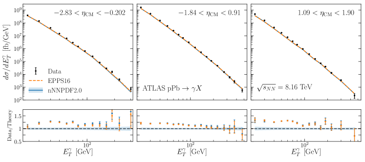
From this comparison one finds that the theory calculations appears to undershoot the experimental data by roughly $25\%$ in the three rapidity bins for most of the $E_{T}^{\gamma}$ range, both for nNNPDF2.0 and EPPS16. This discrepancy cannot be accommodated within the stated experimental and theoretical uncertainties. A similar qualitative behavior was reported in the original ATLAS publication based on the JETPHOX predictions. On the other hand, the NNPDF3.1 proton PDFs are known to describe well the corresponding isolated photon measurements from proton collisions at both $\sqrt{s}=8$ and 13 TeV Campbell:2018wfu .

As expected, the disagreement between the experimental data and the theory calculations found in Fig. 5.1 is translated into poor $\chi^{2}$ values. Using nNNPDF2.0, one obtains that $\chi^{2}/n_{\rm dat}=9.1,10.5,$ and $8.5$ in the forward, central, and backwards rapidity bin. Similar numbers are obtained in the case of the theory predictions based on EPPS16. The situation does not improve by much if the ATLAS photon data is added to the nNNPDF2.0 global analysis. In such a case the agreement between the theory calculations and the experimental data improves somewhat, with $\chi^{2}/n_{\rm dat}=6.1,7.5,$ and $5.7$ for the three rapidity bins, but it remains far from satisfactory.

Until the origin of this disagreement between theory and data is better understood, it will not be possible to include the ATLAS prompt photon production measurements in a global nPDF fit. Alternatively, one could instead consider fitting related observables that are presented in the same ATLAS publication. The first of these is the nuclear modifications ratio $R_{p{\rm Pb}}$, where the absolute $E_{T}^{\gamma}$ distributions in pPb collisions are normalized to their pp counterparts, the latter being derived from a simulation-derived extrapolation from data in proton-proton collisions at $\sqrt{s}=8$ TeV. The second is the ratio between different rapidity bins, such as between forward and backward rapidities, as a function of $E_{T}^{\gamma}$. The advantages of such ratios is that many experimental systematic uncertainties partially cancel out, thus facilitating the comparison with theoretical predictions. On the other hand, these observables might also exhibit a reduced nPDF sensitivity, in particular for the ratio between different rapidity bins. Future studies should shed more light on the usefulness of the prompt photon measurements to constrain nuclear PDFs within a global analysis.

5.2 Isolated photon production in pA collisions with FoCal

Current measurements of direct photon production at the LHC, such as those discussed above from the ATLAS collaboration Aaboud:2019tab as well as related measurements from CMS and ALICE Acharya:2020sxs , are restricted to the central rapidity region. The reason is that this is the only region instrumented with electromagnetic calorimeters and thus suitable to identify photons. A measurement of isolated photon production in the forward region, however, is also highly interesting for nPDF studies. Not only would such measurements provide direct access to the poorly-known gluon nuclear modifications at small-$x$, but it would also allow testing for the possible onset of QCD non-linear dynamics Benic:2016uku .

With this motivation, a new forward calorimeter extension of the ALICE detector, dubbed FoCal vanderKolk:2020fqo ; ALICECollaboration:2719928 , has been proposed. Both the acceptance and instrumentation of this detector have been optimized to provide access to the nuclear PDFs at low scales and small momentum fractions via the measurement of isolated photon production at low transverse momenta and forward rapidities in proton-ion collisions. The FoCal is proposed for installation during the Long Shutdown 3 (2025-2026) phase of the LHC.

The impact of future FoCal measurements on the small-$x$ nuclear PDFs was first studied in Ref. vanLeeuwen:2019zpz . In that analysis, pseudo-data based on the expected kinematical reach and experimental uncertainties for FoCal was generated and used to constrain the nNNPDF1.0 determination by means of the Bayesian reweighting method Ball:2010gb ; Ball:2011gg . It was found that the FoCal measurement would constrain the nuclear gluon modifications down to $x\simeq 10^{-5}$, leading to an uncertainty reduction by up to an order of magnitude as compared to the baseline fit. These results indicated a comparable or superior constraining power on the small-$x$ nPDFs when compared to related projections from future facilities, such as the Electron Ion Collider Accardi:2012qut .

Motivated by the new and improved projections for the FoCal pseudodata that have recently became available, we revisit their impact on nuclear PDFs using the present nPDF determination. In this case, the nNNPDF2.0 PDFs represent a more realistic baseline since they provide a robust quark flavor separation with a better handle on the gluon. Moreover, the positivity of physical cross-sections is guaranteed, a constraint that helps to reduce the small-$x$ nuclear PDF uncertainties.

For this study we have adopted the same settings as in Ref. vanLeeuwen:2019zpz and computed NLO QCD predictions with a modified version of INCNLO that benefits from improved numerical stability at forward rapidities Helenius:2014qla . Theoretical predictions for FoCal cross-sections have been computed with $N_{\rm rep}=400$ replicas of nNNPDF2.0, which are subsequently used to account for the impact of the FoCal pseudo-data by means of Bayesian reweighting. Fig. 5.2 displays the nuclear modification factor $R_{\rm pPb}(p_{T}^{\gamma})$ for direct photon production in pPb collisions at $\sqrt{s}=8.8$ TeV for a rapidity of $\eta_{\gamma}=4.5$ as a function of the photon’s transverse momentum $p_{T}^{\gamma}$. The theoretical predictions based on NLO QCD theory are compared with the FoCal pseudo-data for two sets of input nPDFs: the original nNNPDF2.0 set, and the variant that has been reweighted with the FoCal projections. Here the central value of the FoCal pseudo-data has been chosen to be the same as that of the nNNPDF2.0 prediction. In the right panel of Fig. 5.2 we show the gluon nuclear modification factor $R_{g}(x,Q)$ for $Q^{2}=10$ GeV² for both the original and the reweighted nNNPDF2.0 fits. In all cases, the nPDF uncertainty bands correspond to the 90% confidence level intervals.

Figure 5.2: Left: the nuclear modification factor $R_{\rm pPb}(p_{T}^{\gamma})$ for direct photon production in pPb collisions at $\sqrt{s}=8.8$ TeV for a rapidity of $\eta_{\gamma}=4.5$ as a function of the photon transverse momentum $p_{T}^{\gamma}$. The theoretical predictions are compared with the FoCal pseudo-data for two sets of input nPDFs: the original nNNPDF2.0 set, and the variant that has been reweighted with with FoCal projections. Here the FoCal pseudo data assumes the central value of the nNNPDF2.0 prediction. Right: the gluon nuclear modification factor $R_{g}(x,Q)$ for $Q^{2}=10$ GeV² for both the original and the reweighted nNNPDF2.0 fits. The nPDF uncertainties correspond in both cases to the 90% confidence level intervals.

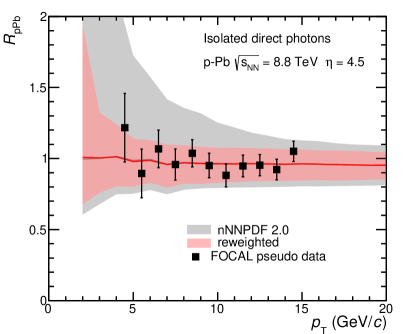
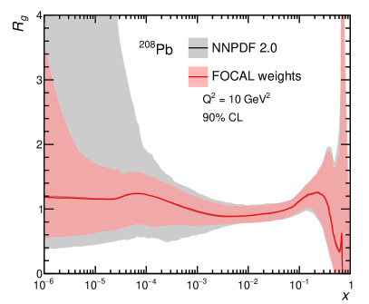
From the results of Fig. 5.2, one finds that the FoCal measurements would still impact the uncertainties of the nuclear gluon modifications at small-$x$, especially in the upper limit of the uncertainty band. The effective number of replicas in this case is $N_{\rm eff}=345$. Note that nNNPDF2.0 exhibits a preference for $R_{\rm pPb}\simeq 1$, and thus shadowing is not favored in the gluon sector, consistent with the results reported in Fig. 4.6. On the other hand, nNNPDF2.0 does not contain any dataset with particular sensitivity to the nuclear gluon modifications, implying that the projections for the impact of FoCal in the global nPDF analysis could be somewhat over-optimistic (see also the discussion in Sect. 6).

Crucially, however, we have assumed in this exercise that the central value of the FoCal measurement would be unchanged compared to the initial baseline prediction. In Fig. 5.3 we display instead the results of the reweighting for a scenario in which the FoCal pseudodata have a value of $R_{\rm pPb}\simeq 0.6$. In this case, the effective number of replicas is much smaller, $N_{\rm eff}=117$, indicating that the FoCal data are adding a significant amount of new information to the global fit. Here the resulting value for the gluon nuclear modification ratio at small-$x$ would be $R_{g}\simeq 0.7$. Therefore, this analysis indicates that FoCal measurements could be sensitive either to the gluon shadowing effects or to possible non-linear QCD dynamics. To disentangle one from the other, a dedicated analysis of the $\chi^{2}$ and nPDF behavior in the small-$x$ region would be required, following the approach developed in Ref. Ball:2017otu .

Figure 5.3: Same as Fig. 5.2 now for the case where the FoCal pseudo data has been generated under the assumption that $R_{\rm pPb}\simeq 0.6$ rather than based on the nNNPDF2.0 central value.

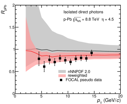
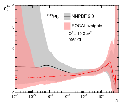
5.3 Inclusive hadron production in pA collisions

The inclusive production of pions and kaons in hadronic collisions provides information not only on the initial state (parton distribution functions) but also on the final-state hadronization mechanism of partons into hadrons. The latter is described by the fragmentation functions (FFs), which are extracted from experimental data by means of a global analysis akin to that of the PDFs deFlorian:2014xna ; Sato:2019yez ; d'Enterria:2013vba ; Bertone:2018ecm ; Bertone:2017tyb ; Albino:2005me ; Hirai:2007cx . Likewise, in proton-nuclear collisions the production of identified hadrons can provide information on the initial state nuclear PDFs as well the parton-to-hadron hadronization in the presence of cold nuclear matter effects.

In Fig. 5.4, we display the nuclear modification ratio $R_{\rm Pb}^{\pi^{0}}$ for the production of neutral pions in proton-lead collisions as a function of the pion transverse momentum $p_{T}$. The theoretical calculations are based on NLO QCD and use the DSS14 hadron fragmentation functions deFlorian:2014xna for both the nNNPDF2.0 and EPPS16 predictions. Moreover, the central values and 90% CL uncertainties are provided for RHIC kinematics, corresponding to $\sqrt{s}=200$ GeV, and for LHC kinematics, where $\sqrt{s}=8.16$ TeV. In both cases, the pions are assumed to be measured at central rapidities, $y_{\pi^{0}}=0$. See Refs. d'Enterria:2013vba ; Albacete:2017qng for additional details regarding the theoretical calculation of inclusive pion production in hadronic collisions.

Figure 5.4: The nuclear modification ratio $R_{\rm Pb}^{\pi^{0}}$ for the production of neutral pions in proton-lead collisions as a function of the pion transverse momentum $p_{T}$. We provide theoretical predictions based on NLO QCD and the DSS14 hadron fragmentation functions both for nNNPDF2.0 and EPPS16, with the corresponding nPDF uncertainties in each case. Results are provided for the RHIC kinematics (left), corresponding to $\sqrt{s}=200$ GeV, and for the LHC kinematics (right), where $\sqrt{s}=8.16$ TeV, and in both cases pions are produced centrally, $|y_{\pi^{0}}|=0$.

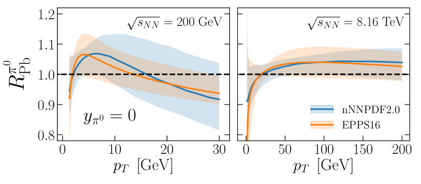
From Fig. 5.4 we can see that the nNNPDF2.0 prediction for $R_{\rm Pb}^{\pi^{0}}$ is consistent with unity within uncertainties for all values of $p_{T}$ both at RHIC and LHC kinematics. At RHIC kinematics, we find that the ratio is less than one at the smallest $p_{T}$ values, becomes $R>1$ between $p_{T}=3$ and 17 GeV, and then goes back to $R<1$. Since inclusive hadron production is dominated by quark-gluon scattering, in particular the scattering of valence quarks for neutral pion production, this behavior is consistent with the results shown in Fig. 4.8. From low to high $p_{T}$, one moves from the shadowing region to the anti-shadowing enhancement, and ends in the region sensitive to EMC suppression. A similar explanation can be made for the trends in $R_{\rm Pb}^{\pi^{0}}$ at the LHC kinematics. However, here the ratio $p_{T}/\sqrt{s}$ does not become large enough to reach the EMC region, and thus the ratio remains larger than one for most of the $p_{T}$ range as a result of anti-shadowing effects. Lastly, the EPPS16 predictions agree with the nNNPDF2.0 result well within uncertainties, reflecting the underlying consistency at the nPDF level.

Overall, the results of Fig. 5.4 confirm that inclusive hadron production in proton-nucleus collisions can provide a handle on the nuclear PDF modifications at medium and large-$x$, although an optimal interpretation of the experimental data can only be achieved by the simultaneous determination of the nPDFs together with the hadron fragmentation functions.

6 Summary and outlook

In this work we have presented a model-independent global determination of nuclear parton distributions by incorporating the constraints from nuclear DIS structure functions and gauge boson production in proton-lead collisions. We have demonstrated that a satisfactory description of all the fitted data sets can be achieved, highlighting the reliability of the QCD factorization paradigm in the heavy nuclear sector. Our results demonstrate significant nuclear effects among the quark flavors in nuclei, in particular a shadowing of the up and down quark distributions in heavy nuclei such as lead. Nuclear modifications are found also in the strangeness of heavier nuclei, displaying a suppression with respect to the free proton across a large region of $x$. In addition, we have shown that upon releasing the momentum and valence sum rule constraints, the data prefer integral values that agree with QCD expectations for all values of $A$.

We have also explored some phenomenological implications of the nNNPDF2.0 determination. We first compared nNNPDF2.0 theoretical predictions with ATLAS measurements of isolated photon production at the LHC, an important hard probe in proton-lead collisions. We then studied the impact on the small-$x$ nuclear gluon PDF from the forward isolated photons production at the FoCal upgrade of the ALICE detector. Lastly, we analyzed our theory predictions for neutral pion production in proton-lead collisions at RHIC and LHC center-of-mass energies. Apart from these applications, the nNNPDF2.0 PDF set can be used as input to theoretical predictions for a range of other hard processes in pPb and PbPb collisions, in particular for heavy ion collisions involving lighter nuclei, in comparisons with non-perturbative nuclear models, and with QCD calculations at small-$x$ involving dense nuclear matter. We also expect the nNNPDF2.0 release to be used in future proton global PDF fits to estimate the theory uncertainties associated with neutrino scattering data Ball:2018twp , and also in high-energy astroparticle physics processes that involve hard scattering on nuclei Garcia:2020jwr ; Bertone:2018dse .

While the input data set used in this work allowed for a state-of-the-art determination of the nuclear quarks and anti-quarks, it only provided loose constraints on the nuclear gluon PDF, especially for heavier nuclei where uncertainties are relatively large. To bypass this limitation, the next step in the nNNPDF family of nuclear PDF fits will be to include additional datasets that provide direct information on the nuclear gluon modifications. In addition to the isolated photon production measurements discussed in Sect. 5.1, perhaps the most attractive candidate in this respect is dijet production in pPb collisions. Measurements of dijet production from Run I in pp collisions have been recently analyzed in the framework of NNLO QCD theory in Ref. AbdulKhalek:2020jut , demonstrating a good compatibility with the global dataset and a marked constraining power on the large-$x$ gluon. In the corresponding pPb case, an EPPS16-based profiling analysis Eskola:2019dui of CMS dijet data at $\sqrt{s}=5.02$ TeV Sirunyan:2018qel revealed a significant pull of this measurement on the nuclear gluon modifications.

Another process that is known to provide important information on the nuclear gluon PDF is charmed meson production, in particular from the LHCb measurements in the forward region Aaij:2017gcy . This process offers unique sensitivity to the small-$x$ (n)PDFs down to $x\simeq 10^{-6}$, as was demonstrated by proton Zenaiev:2015rfa ; Bertone:2018dse ; Gauld:2016kpd and nuclear studies Kusina:2017gkz ; Eskola:2019bgf . Fully exploiting the constraints provided by these measurements requires, as for the rest of hard probes in nuclear collisions, a consistent theoretical and methodological treatment of charm production in both proton and nuclear global QCD analyses.

On a longer timescale, one might aim to achieve a determination of the proton and nuclear PDFs simultaneously from a universal analysis, thus bypassing the need to include proton information by means of the proton boundary condition penalty. In the same spirit of the QCD analyses of proton PDFs and fragmentation functions presented in Refs. Sato:2019yez ; Ethier:2017zbq , such an integrated fit of proton and nuclear PDFs would ensure the ultimate theoretical and methodological consistency of the determination of the nuclear modifications of the free-nucleon quark and gluon structure.
 

The nNNPDF2.0 determination is available in the LHAPDF6 library Buckley:2014ana for all relevant nuclei from $A=1$ to $A=208$. The nNNPDF2.0 sets are available both for the nPDFs of bound protons, $f^{(p/A)}(x,Q^{2})$, and those of bound nucleons, $f^{(N/A)}(x,Q^{2})$, following the conventions in Sect. 3.1. Each of these sets is composed by $N_{\rm rep}=250$ correlated replicas, see Sect. 5 of AbdulKhalek:2019mzd for their usage prescriptions. The naming convention used for the sets is the following:

$\qquad\qquad f^{(N/A)}(x,Q^{2})$	$\qquad\qquad f^{(p/A)}(x,Q^{2})$
nNNPDF20_nlo_as_0118_N1	nNNPDF20_nlo_as_0118_N1
nNNPDF20_nlo_as_0118_D2	nNNPDF20_nlo_as_0118_p_A2_Z1
nNNPDF20_nlo_as_0118_He4	nNNPDF20_nlo_as_0118_p_A4_Z2
nNNPDF20_nlo_as_0118_Li6	nNNPDF20_nlo_as_0118_p_A6_Z3
nNNPDF20_nlo_as_0118_Be9	nNNPDF20_nlo_as_0118_p_A9_Z4
nNNPDF20_nlo_as_0118_C12	nNNPDF20_nlo_as_0118_p_A12_Z6
nNNPDF20_nlo_as_0118_N14	nNNPDF20_nlo_as_0118_p_A14_Z7
nNNPDF20_nlo_as_0118_Al27	nNNPDF20_nlo_as_0118_p_A27_Z13
nNNPDF20_nlo_as_0118_Ca40	nNNPDF20_nlo_as_0118_p_A40_Z20
nNNPDF20_nlo_as_0118_Fe56	nNNPDF20_nlo_as_0118_p_A56_Z26
nNNPDF20_nlo_as_0118_Cu64	nNNPDF20_nlo_as_0118_p_A64_Z29
nNNPDF20_nlo_as_0118_Ag108	nNNPDF20_nlo_as_0118_p_A108_Z47
nNNPDF20_nlo_as_0118_Sn119	nNNPDF20_nlo_as_0118_p_A119_Z50
nNNPDF20_nlo_as_0118_Xe131	nNNPDF20_nlo_as_0118_p_A131_Z54
nNNPDF20_nlo_as_0118_Au197	nNNPDF20_nlo_as_0118_p_A197_Z79
nNNPDF20_nlo_as_0118_Pb208	nNNPDF20_nlo_as_0118_p_A208_Z82

Additional variants of the nNNPDF2.0 NLO fit present in this work, such as the fits without the momentum and valence sum rules and a $N_{\rm rep}=1000$ replica set for lead, are available on the NNPDF collaboration website:

http://nnpdf.mi.infn.it/for-users/nuclear-pdf-sets/

Acknowledgments

We are grateful to our colleagues of the NNPDF collaboration for support and stimulating discussions, and in particular to Emanuele R. Nocera for his continuous assistance during this work. We thank Kari Eskola, Petja Paakkinen, and Hannu Paukkunen for discussions about the EPPS16 analysis. We thank Marco van Leeuwen for providing the predictions for FoCal and Ilkka Helenius for those of pion production in heavy ion collisions. R. A. K., J. E., and J. R. are supported by the Netherlands Organization for Scientific Research (NWO). We acknowledge grants of computer capacity from the Finnish Grid and Cloud Infrastructure (persistent identifier urn:nbn:fi:research-infras-2016072533).

Appendix A PDF sensitivity of input cross-sections

In this appendix we indicate the PDF sensitivity of all processes used as input in the nNNPDF2.0 determination by providing their explicit cross-section expressions at leading order (LO) in perturbative QCD. We provide these expressions for a general nuclear target with $Z$ protons and $(A-Z)$ neutrons in terms of bound proton distributions of the physical and evolution bases, and in terms of the average bound nucleon PDFs. In what follows, we further simplify the conventions adopted in Sect. 3.1 to

$$f \equiv f^{(p/A)}\,,$$ (A.1)

$$f_{A} \equiv f^{(N/A)}\,.$$ (A.2)

1. Lepton-nucleus scattering.

The double differential cross-section for the DIS of a charged lepton off a nucleus with mass number $A$ is given by

$${{d^{2}\sigma^{i,l^{\pm}}}\over{dxdQ^{2}}}(x,Q^{2},A)={{2\pi\alpha^{2}}\over{xQ^{4}}}\eta^{i}\left[Y_{+}F_{2}^{i}(x,Q^{2},A)\mp Y_{-}xF_{3}^{i}(x,Q^{2},A)-y^{2}F_{L}^{i}(x,Q^{2},A)\right]\,,$$ (A.3)

with $i=\rm NC,\,CC$, $\eta^{\rm NC}=1$, $\eta^{\rm CC}=(1\pm\lambda)^{2}\eta_{W}$, where $\eta_{W}$ denotes the squared ratio of the W-boson couplings and propagator with respect to those of the photon, and $\lambda$ is the helicity of the incoming lepton. In the case of NC DIS we restrict ourselves to photon-mediated processes, for which $F^{\rm NC}_{3}=0$. The usual DIS kinematic variables are defined as $Y_{\pm}=1\pm(1-y)^{2}$ and

$$x={{Q^{2}}\over{2P\cdot q}},\quad Q^{2}=-q^{2},\quad y={{q\cdot P}\over{k\cdot P}}\,.$$ (A.4)

A1. Neutral-current DIS.

For NC DIS, the underlying process is lepton-nucleus scattering mediated by a virtual photon exchange, $l^{\pm}+A\xrightarrow[]{\gamma}l^{\pm}+X$. Since the available data is at $Q^{2}<<M_{Z}$, the contributions from $Z$ boson exchange can be neglected. The double-differential cross-section for the scattering of a charged lepton off a nucleus with atomic and mass numbers $Z$ and $A$ is proportional at leading order to the $F_{2}$ structure function which can be expressed as

$$\begin{split}F_{2}^{\rm NC}&={{x}\over{9A}}\bigg{[}(4A-3Z)d^{+}+As^{+}+(A+3Z)u^{+}\bigg{]}={{x}\over{9}}\bigg{[}4u^{+}_{A}+d^{+}_{A}+s^{+}_{A}\bigg{]}\\ &={{x}\over{18A}}\bigg{[}4A\Sigma+AT_{8}+3(2Z-A)T_{3}\bigg{]}\,,\end{split}$$ (A.5)

Here we define the structure function per nucleon, rather than the structure function of the nucleus as a whole. We can see from the above expression that for an isoscalar nucleus $A=2Z$ the contribution proportional to $T_{3}$ vanishes and the nuclear structure functions depend only on $\Sigma$ and $T_{8}$ via the $\Sigma+T_{8}$ combination. At LO only Eq. (A.5) is relevant for the description of neutral-current DIS since the longitudinal structure function vanishes due to the Callan-Gross relation, $F_{L}^{\rm NC}=F_{2}^{\rm NC}-2xF_{1}^{\rm NC}=0$.

B1. Charged-current DIS.

For CC DIS, the underlying process is neutrino scattering off of a nucleus via the exchange of a W boson, $\nu+A\xrightarrow[]{W^{-}}l^{-}+X$ and $\bar{\nu}+A\xrightarrow[]{W^{+}}+l^{+}+X$. Due to the fact that W⁺ and W^- bosons couple to different quark flavors, the difference between neutrino and anti-neutrino structure functions provides a handle on quark flavor separation. Here we provide the expressions for $\nu(\bar{nu})A$ scattering, the expressions for the conjugate process involving the CC scattering of charged leptons is the same. The expressions for the inclusive CC structure functions via $W^{-}$-boson exchange, $\bar{\nu}+A\xrightarrow[]{W^{-}}+l^{+}X$, are the following:

$$\begin{split}F_{2}^{\bar{\nu}A\xrightarrow[]{W^{-}}l^{+}X}={{2x}\over{A}}\bigg{[}&|V_{ud}|^{2}\bigg{(}Z(u+\bar{d})+(A-Z)(d+\bar{u})\bigg{)}+|V_{us}|^{2}\bigg{(}Zu+(A-Z)d+A\bar{s}\bigg{)}\bigg{]}\\ =2x\bigg{[}&|V_{ud}|^{2}\bigg{(}u_{A}+\bar{d}_{A}\bigg{)}+|V_{us}|^{2}\bigg{(}u_{A}+\bar{s_{A}}\bigg{)}\bigg{]}\\ ={{x}\over{6A}}\bigg{[}&|V_{ud}|^{2}\bigg{(}2A(2\Sigma+T_{8})+6(2Z-A)V_{3}\bigg{)}\\ +&|V_{us}|^{2}\bigg{(}3(2Z-A)T_{3}+3(2Z-A)V_{3}+A(4\Sigma-T_{8}+3V_{8})\bigg{)}\bigg{]}\end{split}$$ (A.6)

$$\begin{split}F_{3}^{\bar{\nu}A\xrightarrow[]{W^{-}}l^{+}X}={{2}\over{A}}\bigg{[}&|V_{ud}|^{2}\bigg{(}Z(u-\bar{d})+(A-Z)(d-\bar{u})\bigg{)}+|V_{us}|^{2}\bigg{(}Zu+(A-Z)d-A\bar{s}\bigg{)}\bigg{]}\\ =2\bigg{[}&|V_{ud}|^{2}\bigg{(}u_{A}-\bar{d}_{A}\bigg{)}+|V_{us}|^{2}\bigg{(}u_{A}-\bar{s_{A}}\bigg{)}\bigg{]}\\ ={{-1}\over{6A}}\bigg{[}&|V_{ud}|^{2}\bigg{(}6(A-2Z)T_{3}-2A(2V+V_{8})\bigg{)}\\ +&|V_{us}|^{2}\bigg{(}+3(A-2Z)T_{3}+3(A-2Z)V_{3}+A(-3T_{8}-4V+V_{8})\bigg{)}\bigg{]}\end{split}$$ (A.7)

Here we consider only the contribution from up-, down-, and strange-initiated processes for simplicity. The generalization to heavy-quark initiated processes is straightforward. An interesting observation from these expressions is that $F_{2}$ and $F_{3}$ provide complementary information on quark flavor separation.

The corresponding expressions for the inclusive charged-current structure functions in the case of neutrino scattering via $W^{+}$-boson exchange, $\nu+A\xrightarrow[]{W^{+}}+l^{-}X$, are given by

$$\begin{split}F_{2}^{\nu A\xrightarrow[]{W^{+}}l^{-}X}={{2x}\over{A}}\bigg{[}&|V_{ud}|^{2}\bigg{(}Z(\bar{u}+d)+(A-Z)(u+\bar{d})\bigg{)}+|V_{us}|^{2}\bigg{(}Z\bar{u}+(A-Z)\bar{d}+As\bigg{)}\bigg{]}\\ =2x\bigg{[}&|V_{ud}|^{2}\bigg{(}\bar{u}_{A}+d_{A}\bigg{)}+|V_{us}|^{2}\bigg{(}\bar{u}_{A}+s_{A}\bigg{)}\bigg{]}\\ ={{x}\over{6A}}\bigg{[}&|V_{ud}|^{2}\bigg{(}2A(2\Sigma+T_{8})+6(A-2Z)V_{3}\bigg{)}\\ +&|V_{us}|^{2}\bigg{(}A(4\Sigma-T_{8}-3V_{8})+3(2Z-A)T_{3}+3(A-2Z)V_{3}\bigg{)}\bigg{]}\end{split}$$ (A.8)

$$\begin{split}F_{3}^{\nu A\xrightarrow[]{W^{+}}l^{-}X}={{2}\over{A}}\bigg{[}&|V_{ud}|^{2}\bigg{(}Z(d-\bar{u})+(A-Z)(u-\bar{d})\bigg{)}+|V_{us}|^{2}\bigg{(}-Z\bar{u}-(A-Z)\bar{d}+As\bigg{)}\bigg{]}\\ =2\bigg{[}&|V_{ud}|^{2}\bigg{(}-\bar{u}_{A}+d_{A}\bigg{)}+|V_{us}|^{2}\bigg{(}-\bar{u}_{A}+s_{A}\bigg{)}\bigg{]}\\ ={{1}\over{6A}}\bigg{[}&|V_{ud}|^{2}\bigg{(}2A(2V+V_{8})+6(A-2Z)T_{3}\bigg{)}\\ +&|V_{us}|^{2}\bigg{(}A(-3T_{8}+4V-V_{8})+3(A-2Z)T_{3}+3(2Z-A)V_{3}\bigg{)}\bigg{]}\end{split}$$ (A.9)

We now turn to the exclusive CC charm production structure functions, required for the description of the NuTeV cross-sections. Following the FONLL treatment of heavy quark structure functions, the charm contribution to the inclusive structure function is defined by all terms where the charm quark couples to the W boson. Note that this definition is somewhat different from the experimental definition, where charm structure functions are identified by requesting the presence of charm in the final state, while the theory definition includes charm-initiated contributions as well. The charm production structure functions in the case of antineutrino- and neutrino-initiated scattering reads for $W^{-}$ as

$$\begin{split}F_{2}^{\bar{\nu}A\xrightarrow[]{W^{-}}l^{+}cX}={{2x}\over{A}}\bigg{[}&|V_{cd}|^{2}\bigg{(}Z\bar{d}+(A-Z)\bar{u}\bigg{)}+|V_{cs}|^{2}A\bar{s}\bigg{]}\\ =2x\bigg{[}&|V_{cd}|^{2}\bar{d}_{A}+|V_{cs}|^{2}\bar{s}_{A}\bigg{]}\\ ={{x}\over{6A}}\bigg{[}&|V_{cd}|^{2}\bigg{(}A(2\Sigma+T_{8}-2V-V_{8})+3(A-2Z)T_{3}+3(2Z-A)V_{3}\bigg{)}\\ +&|V_{cs}|^{2}2A\bigg{(}\Sigma-T_{8}-V+V_{8}\bigg{)}\bigg{]}\end{split}$$ (A.10)

$$\begin{split}F_{3}^{\bar{\nu}A\xrightarrow[]{W^{-}}l^{+}cX}={{2}\over{A}}\bigg{[}&|V_{cd}|^{2}\bigg{(}-Z\bar{d}-(A-Z)\bar{u}\bigg{)}-|V_{cs}|^{2}A\bar{s}\bigg{]}\\ =-2\bigg{[}&|V_{cd}|^{2}\bar{d}_{A}+|V_{cs}|^{2}\bar{s}_{A}\bigg{]}\\ ={{-1}\over{6A}}\bigg{[}&|V_{cd}|^{2}\bigg{(}3(A-2Z)T_{3}+3(2Z-A)V_{3}+A(2\Sigma+AT_{8}-2AV-AV_{8})\bigg{)}\\ +&|V_{cs}|^{2}2A\bigg{(}+\Sigma-T_{8}-V+V_{8}\bigg{)}\bigg{]}\end{split}$$ (A.11)

and for $W^{+}$:

$$\begin{split}F_{2}^{\nu A\xrightarrow[]{W^{+}}l^{-}cX}={{2x}\over{A}}\bigg{[}&|V_{cd}|^{2}\bigg{(}Zd+(A-Z)u\bigg{)}+|V_{cs}|^{2}As\bigg{]}\\ =2x\bigg{[}&|V_{cd}|^{2}d_{A}+|V_{cs}|^{2}s_{A}\bigg{]}\\ ={{x}\over{6A}}\bigg{[}&|V_{cd}|^{2}\bigg{(}A(2\Sigma+T_{8}+2V+V_{8})+3(A-2Z)T_{3}+3(A-2Z)V_{3}\bigg{)}\\ +&|V_{cs}|^{2}2A\bigg{(}+\Sigma-T_{8}+V-V_{8}\bigg{)}\bigg{]}\end{split}$$ (A.12)

$$\begin{split}F_{3}^{\nu A\xrightarrow[]{W^{+}}l^{-}cX}={{-2}\over{A}}\bigg{[}&|V_{cd}|^{2}\bigg{(}+Zd+(A-Z)u\bigg{)}+|V_{cs}|^{2}As\bigg{]}\\ =-2\bigg{[}&|V_{cd}|^{2}d_{A}+|V_{cs}|^{2}s_{A}\bigg{]}\\ ={{-1}\over{6A}}\bigg{[}&|V_{cd}|^{2}\bigg{(}A(2\Sigma+T_{8}+2V+V_{8})+3(A-2Z)T_{3}+3(A-2Z)V_{3}\bigg{)}\\ +&|V_{cs}|^{2}2A\bigg{(}+\Sigma-T_{8}+V-V_{8}\bigg{)}\bigg{]}\end{split}$$ (A.13)

2. Weak boson production.

Here we provide the corresponding leading order expressions for weak gauge boson production in proton-nucleus collisions. Experimental measurements for NC observables are provided in terms of the invariant mass $M$ and rapidity of the dilepton final state, while CC measurements are binned in terms of the charged lepton rapidity. Here we show the LO expressions without accounting for the gauge boson decay, so in the case of W^± production the connection with the experimental data is somewhat less direct than for $Z$ boson production.

A2. Neutral current DY

We start by discussing NC Drell-Yan (DY), namely $Z$-boson production in proton-nucleus collisions, $p+A\xrightarrow[]{Z}l^{+}l^{-}$. The leading order expressions are given by

$$\begin{split}{{d\sigma_{Z}^{pA}}\over{dM^{2}dy}}&\propto A\bigg{[}a_{u}\bigg{(}u_{1}\bar{u}_{2}+\bar{u}_{1}u_{2}\bigg{)}+a_{d}\bigg{(}d_{1}\bar{d}_{2}+\bar{d}_{1}d_{2}+s_{1}\bar{s}_{2}+\bar{s}_{1}s_{2}\bigg{)}\bigg{]}\end{split}$$ (A.14)

where $q_{1}=q(x_{1},M^{2})$ and $q_{2}=q(x_{2},M^{2})$ and the Drell-Yan kinematics at LO are:

$$x_{1,2}={{M}\over{\sqrt{s}}}e^{\pm y}\,,\quad\quad M^{2}=x_{1}x_{2}s\,,$$ (A.15)

with $\sqrt{s}$ being the center-of-mass energy of the collision, $M$ being the invariant mass of the final state, and $y$ the rapidity of the final state system. The effective weak couplings are given by

$$a_{q}=(\bar{g}^{q}_{V}+\bar{g}^{q}_{A}),\quad\quad\bar{g}^{f}_{V}=(t^{(f)}_{3}-2Q_{f}\sin^{2}\theta_{W}),\quad\quad\bar{g}^{f}_{A}=t^{(f)}_{3}$$

where $t^{(f)}_{3}$ is the weak isospin of fermion $f$, $Q_{f}$ is the electric charge and $\theta_{W}$ is Weinberg’s angle.

B2. Charged current DY

The corresponding LO expressions in the case of W^- and W⁺ boson production in pA collisions are given by

$$\begin{split}{{d\sigma_{W^{-}}^{pA,}}\over{dM^{2}dy}}\propto\,\,&|V_{ud}|^{2}\bigg{(}Z(d_{1}\bar{u}_{2}+\bar{u}_{1}d_{2})+(A-Z)(\bar{d}_{1}u_{2}+u_{1}\bar{d}_{2})\bigg{)}\\ +&|V_{us}|^{2}\bigg{(}Z(d_{1}\bar{s}_{2}+\bar{s}_{1}d_{2})+(A-Z)(u_{1}\bar{s}_{2}+\bar{s}_{1}u_{2})\bigg{)}\end{split}$$ (A.16)

and:

$$\begin{split}{{d\sigma_{W^{+}}^{pA,}}\over{dM^{2}dy}}\propto\,\,&|V_{ud}|^{2}\bigg{(}Z(u_{1}\bar{d}_{2}+\bar{d}_{1}u_{2})+(A-Z)(d_{1}\bar{u}_{2}+\bar{u}_{1}d_{2})\bigg{)}\\ +&|V_{us}|^{2}\bigg{(}Z(u_{1}\bar{s}_{2}+\bar{s}_{1}u_{2})+(A-Z)(d_{1}\bar{s}_{2}+\bar{s}_{1}d_{2})\bigg{)}\end{split}$$ (A.17)

where in this case $y$ stands for the $W$ boson rapidity, which in general is different from the pseudo-rapidity of the charged lepton that is measured by experiments. However, in either case the PDF combinations that enter at LO remain the same. From the comparison between the LO expressions of the DIS structure functions and the $W$ and $Z$ production cross-sections in pA collisions, it is clear that each group of process is sensitive to a different combination of quark and antiquark PDFs. Therefore, their combination (due to the PDF universality in QCD) into a global QCD analysis provides a unique handle for a robust separation between quark and antiquark flavors in nuclei.

References

- (1) J. Rojo, The Partonic Content of Nucleons and Nuclei, arXiv:1910.03408.
- (2) J. J. Ethier and E. R. Nocera, Parton Distributions in Nucleons and Nuclei, Ann. Rev. Nucl. Part. Sci. (2020), no. 70 1–34, [arXiv:2001.07722].
- (3) J. Gao, L. Harland-Lang, and J. Rojo, The Structure of the Proton in the LHC Precision Era, Phys. Rept. 742 (2018) 1–121, [arXiv:1709.04922].
- (4) N. Armesto, N. Borghini, S. Jeon, U. A. Wiedemann, S. Abreu, V. Akkelin, J. Alam, J. L. Albacete, A. Andronic, D. Antonov, et al., Heavy Ion Collisions at the LHC - Last Call for Predictions, J. Phys. G35 (2008) 054001, [arXiv:0711.0974].
- (5) STAR Collaboration, J. Adams et al., Experimental and theoretical challenges in the search for the quark gluon plasma: The STAR Collaboration’s critical assessment of the evidence from RHIC collisions, Nucl. Phys. A757 (2005) 102–183, [nucl-ex/0501009].
- (6) NNPDF Collaboration, R. D. Ball et al., Parton distributions for the LHC Run II, JHEP 04 (2015) 040, [arXiv:1410.8849].
- (7) T.-J. Hou et al., New CTEQ global analysis of quantum chromodynamics with high-precision data from the LHC, arXiv:1912.10053.
- (8) L. A. Harland-Lang, A. D. Martin, P. Motylinski, and R. S. Thorne, Parton distributions in the LHC era: MMHT 2014 PDFs, Eur. Phys. J. C75 (2015) 204, [arXiv:1412.3989].
- (9) S. Alekhin, J. Blümlein, S. Moch, and R. Placakyte, Parton distribution functions, , and heavy-quark masses for LHC Run II, Phys. Rev. D96 (2017), no. 1 014011, [arXiv:1701.05838].
- (10) NNPDF Collaboration, R. D. Ball, E. R. Nocera, and R. L. Pearson, Nuclear Uncertainties in the Determination of Proton PDFs, Eur. Phys. J. C79 (2019), no. 3 282, [arXiv:1812.09074].
- (11) K. J. Eskola, P. Paakkinen, H. Paukkunen, and C. A. Salgado, EPPS16: Nuclear parton distributions with LHC data, Eur. Phys. J. C77 (2017), no. 3 163, [arXiv:1612.05741].
- (12) K. Kovarik et al., nCTEQ15 - Global analysis of nuclear parton distributions with uncertainties in the CTEQ framework, Phys. Rev. D93 (2016), no. 8 085037, [arXiv:1509.00792].
- (13) NNPDF Collaboration, R. Abdul Khalek, J. J. Ethier, and J. Rojo, Nuclear parton distributions from lepton-nucleus scattering and the impact of an electron-ion collider, Eur. Phys. J. C79 (2019), no. 6 471, [arXiv:1904.00018].
- (14) M. Walt, I. Helenius, and W. Vogelsang, Open-source QCD analysis of nuclear parton distribution functions at NLO and NNLO, Phys. Rev. D100 (2019), no. 9 096015, [arXiv:1908.03355].
- (15) H. Khanpour and S. Atashbar Tehrani, Global Analysis of Nuclear Parton Distribution Functions and Their Uncertainties at Next-to-Next-to-Leading Order, Phys. Rev. D93 (2016), no. 1 014026, [arXiv:1601.00939].
- (16) ALICE Collaboration, J. Adam et al., Measurement of charged jet production cross sections and nuclear modification in p-Pb collisions at TeV, Phys. Lett. B749 (2015) 68–81, [arXiv:1503.00681].
- (17) ALICE Collaboration, J. Adam et al., Multiplicity dependence of charged pion, kaon, and (anti)proton production at large transverse momentum in p-Pb collisions at = 5.02 TeV, Phys. Lett. B760 (2016) 720–735, [arXiv:1601.03658].
- (18) ALICE Collaboration, J. Adam et al., Measurement of dijet in p–Pb collisions at =5.02 TeV, Phys. Lett. B746 (2015) 385–395, [arXiv:1503.03050].
- (19) ATLAS Collaboration, G. Aad et al., Transverse momentum, rapidity, and centrality dependence of inclusive charged-particle production in TeV + Pb collisions measured by the ATLAS experiment, Phys. Lett. B 763 (2016) 313–336, [arXiv:1605.06436].
- (20) CMS Collaboration, S. Chatrchyan et al., Studies of dijet transverse momentum balance and pseudorapidity distributions in pPb collisions at TeV, Eur. Phys. J. C74 (2014), no. 7 2951, [arXiv:1401.4433].
- (21) ALICE Collaboration, J. Zhu, Measurement of w-boson production in p–pb collisions at = 5.02 tev with alice at the lhc, Journal of Physics: Conference Series 612 (2015), no. 1 012009.
- (22) Measurement of production in +Pb collision at TeV with ATLAS detector at the LHC, Tech. Rep. ATLAS-CONF-2015-056, CERN, Geneva, Sep, 2015.
- (23) ATLAS Collaboration, G. Aad et al., boson production in Pb collisions at TeV measured with the ATLAS detector, Phys. Rev. C92 (2015), no. 4 044915, [arXiv:1507.06232].
- (24) CMS Collaboration, V. Khachatryan et al., Study of Z boson production in pPb collisions at =5.02TeV, Phys. Lett. B759 (2016) 36–57, [arXiv:1512.06461].
- (25) CMS Collaboration, V. Khachatryan et al., Study of W boson production in pPb collisions at 5.02 TeV, Phys. Lett. B750 (2015) 565–586, [arXiv:1503.05825].
- (26) CMS Collaboration, S. Chatrchyan et al., Charm-tagged jet production in pPb collisions at 5.02 TeV and pp collisions at 2.76 TeV, CMS-PAS-HIN-15-012.
- (27) ALICE Collaboration, J. Adam et al., Measurement of D-meson production versus multiplicity in p-Pb collisions at TeV, JHEP 08 (2016) 078, [arXiv:1602.07240].
- (28) ALICE Collaboration, J. Adam et al., Measurement of electrons from heavy-flavour hadron decays in p-Pb collisions at 5.02 TeV, Phys. Lett. B754 (2016) 81–93, [arXiv:1509.07491].
- (29) ALICE Collaboration, B. B. Abelev et al., Measurement of prompt -meson production in collisions at = 5.02 TeV, Phys. Rev. Lett. 113 (2014), no. 23 232301, [arXiv:1405.3452].
- (30) CMS Collaboration, V. Khachatryan et al., Transverse momentum spectra of inclusive b jets in pPb collisions at 5.02 TeV, Phys. Lett. B754 (2016) 59, [arXiv:1510.03373].
- (31) CMS Collaboration, V. Khachatryan et al., Study of B Meson Production in pPb Collisions at 5.02 TeV Using Exclusive Hadronic Decays, Phys. Rev. Lett. 116 (2016), no. 3 032301, [arXiv:1508.06678].
- (32) LHCb Collaboration, R. Aaij et al., Study of prompt D0 meson production in Pb collisions at TeV, JHEP 10 (2017) 090, [arXiv:1707.02750].
- (33) LHCb Collaboration, R. Aaij et al., Measurement of , and production in collisions at , Phys. Rev. D99 (2019), no. 5 052011, [arXiv:1902.05599].
- (34) A. Kusina, F. Lyonnet, D. B. Clark, E. Godat, T. Jezo, K. Kovarik, F. I. Olness, I. Schienbein, and J. Y. Yu, Vector boson production in pPb and PbPb collisions at the LHC and its impact on nCTEQ15 PDFs, Eur. Phys. J. C77 (2017), no. 7 488, [arXiv:1610.02925].
- (35) A. Kusina, J.-P. Lansberg, I. Schienbein, and H.-S. Shao, Gluon Shadowing in Heavy-Flavor Production at the LHC, Phys. Rev. Lett. 121 (2018), no. 5 052004, [arXiv:1712.07024].
- (36) N. Armesto, H. Paukkunen, J. M. Penín, C. A. Salgado, and P. Zurita, An analysis of the impact of LHC Run I proton–lead data on nuclear parton densities, Eur. Phys. J. C76 (2016), no. 4 218, [arXiv:1512.01528].
- (37) K. J. Eskola, P. Paakkinen, and H. Paukkunen, Non-quadratic improved Hessian PDF reweighting and application to CMS dijet measurements at 5.02 TeV, Eur. Phys. J. C79 (2019), no. 6 511, [arXiv:1903.09832].
- (38) S. Forte, L. Garrido, J. I. Latorre, and A. Piccione, Neural network parametrization of deep-inelastic structure functions, JHEP 05 (2002) 062, [hep-ph/0204232].
- (39) The NNPDF Collaboration, L. Del Debbio, S. Forte, J. I. Latorre, A. Piccione, and J. Rojo, Unbiased determination of the proton structure function f2(p) with estimation, JHEP 03 (2005) 080, [hep-ph/0501067].
- (40) The NNPDF Collaboration, L. Del Debbio, S. Forte, J. I. Latorre, A. Piccione, and J. Rojo, Neural network determination of parton distributions: The nonsinglet case, JHEP 03 (2007) 039, [hep-ph/0701127].
- (41) The NNPDF Collaboration, R. D. Ball et al., A determination of parton distributions with faithful uncertainty estimation, Nucl. Phys. B809 (2009) 1–63, [arXiv:0808.1231].
- (42) The NNPDF Collaboration, J. Rojo et al., Update on Neural Network Parton Distributions: NNPDF1.1, arXiv:0811.2288.
- (43) The NNPDF Collaboration, R. D. Ball et al., Fitting Parton Distribution Data with Multiplicative Normalization Uncertainties, JHEP 05 (2010) 075, [arXiv:0912.2276].
- (44) The NNPDF Collaboration, R. D. Ball et al., A first unbiased global NLO determination of parton distributions and their uncertainties, Nucl. Phys. B838 (2010) 136, [arXiv:1002.4407].
- (45) The NNPDF Collaboration, R. D. Ball et al., Impact of Heavy Quark Masses on Parton Distributions and LHC Phenomenology, Nucl. Phys. B849 (2011) 296, [arXiv:1101.1300].
- (46) The NNPDF Collaboration, R. D. Ball et al., Unbiased global determination of parton distributions and their uncertainties at NNLO and at LO, Nucl.Phys. B855 (2012) 153, [arXiv:1107.2652].
- (47) R. D. Ball et al., Parton distributions with LHC data, Nucl.Phys. B867 (2013) 244, [arXiv:1207.1303].
- (48) ATLAS Collaboration, M. Aaboud et al., Precision measurement and interpretation of inclusive , and production cross sections with the ATLAS detector, Eur. Phys. J. C 77 (2017), no. 6 367, [arXiv:1612.03016].
- (49) J. Gomez et al., Measurement of the A-dependence of deep inelastic electron scattering, Phys. Rev. D49 (1994) 4348–4372.
- (50) New Muon Collaboration, P. Amaudruz et al., A Reevaluation of the nuclear structure function ratios for D, He, Li-6, C and Ca, Nucl.Phys. B441 (1995) 3–11, [hep-ph/9503291].
- (51) New Muon Collaboration, M. Arneodo et al., The Structure Function ratios F2(li) / F2(D) and F2(C) / F2(D) at small x, Nucl.Phys. B441 (1995) 12–30, [hep-ex/9504002].
- (52) New Muon Collaboration, M. Arneodo et al., The A dependence of the nuclear structure function ratios, Nucl.Phys. B481 (1996) 3–22.
- (53) European Muon Collaboration, J. Ashman et al., Measurement of the Ratios of Deep Inelastic Muon - Nucleus Cross-Sections on Various Nuclei Compared to Deuterium, Phys. Lett. B202 (1988) 603–610.
- (54) European Muon Collaboration, M. Arneodo et al., Measurements of the nucleon structure function in the range and in deuterium, carbon and calcium, Nucl. Phys. B333 (1990) 1–47.
- (55) E665 Collaboration, M. R. Adams et al., Shadowing in inelastic scattering of muons on carbon, calcium and lead at low x(Bj), Z. Phys. C67 (1995) 403–410, [hep-ex/9505006].
- (56) D. M. Alde et al., Nuclear dependence of dimuon production at 800-GeV. FNAL-772 experiment, Phys. Rev. Lett. 64 (1990) 2479–2482.
- (57) European Muon Collaboration, J. J. Aubert et al., Measurements of the nucleon structure functions in deep inelastic muon scattering from deuterium and comparison with those from hydrogen and iron, Nucl. Phys. B293 (1987) 740–786.
- (58) BCDMS Collaboration, A. C. Benvenuti et al., Nuclear Effects in Deep Inelastic Muon Scattering on Deuterium and Iron Targets, Phys. Lett. B189 (1987) 483–487.
- (59) European Muon Collaboration, J. Ashman et al., A Measurement of the ratio of the nucleon structure function in copper and deuterium, Z.Phys. C57 (1993) 211–218.
- (60) New Muon Collaboration, M. Arneodo et al., The dependence of the structure function ratio in deep inelastic muon scattering, Nucl.Phys. B481 (1996) 23–39.
- (61) Fermilab E665 Collaboration, M. R. Adams et al., Shadowing in the muon xenon inelastic scattering cross-section at 490-GeV, Phys. Lett. B287 (1992) 375–380.
- (62) CHORUS Collaboration, G. Onengut et al., Measurement of nucleon structure functions in neutrino scattering, Phys. Lett. B632 (2006) 65–75.
- (63) NuTeV Collaboration, M. Goncharov et al., Precise measurement of dimuon production cross-sections in Fe and Fe deep inelastic scattering at the Tevatron, Phys. Rev. D64 (2001) 112006, [hep-ex/0102049].
- (64) CMS Collaboration, A. M. Sirunyan et al., Observation of nuclear modifications in W± boson production in pPb collisions at 8.16 TeV, Phys. Lett. B800 (2020) 135048, [arXiv:1905.01486].
- (65) V. Bertone, S. Carrazza, and J. Rojo, APFEL: A PDF Evolution Library with QED corrections, Comput.Phys.Commun. 185 (2014) 1647, [arXiv:1310.1394].
- (66) S. Forte, E. Laenen, P. Nason, and J. Rojo, Heavy quarks in deep-inelastic scattering, Nucl. Phys. B834 (2010) 116–162, [arXiv:1001.2312].
- (67) V. Bertone, S. Carrazza, and N. P. Hartland, APFELgrid: a high performance tool for parton density determinations, Comput. Phys. Commun. 212 (2017) 205–209, [arXiv:1605.02070].
- (68) E. L. Berger, J. Gao, C. S. Li, Z. L. Liu, and H. X. Zhu, Charm-Quark Production in Deep-Inelastic Neutrino Scattering at Next-to-Next-to-Leading Order in QCD, Phys. Rev. Lett. 116 (2016), no. 21 212002, [arXiv:1601.05430].
- (69) J. Gao, Massive charged-current coefficient functions in deep-inelastic scattering at NNLO and impact on strange-quark distributions, JHEP 02 (2018) 026, [arXiv:1710.04258].
- (70) R. Boughezal, J. M. Campbell, R. K. Ellis, C. Focke, W. Giele, X. Liu, F. Petriello, and C. Williams, Color singlet production at NNLO in MCFM, Eur. Phys. J. C 77 (2017), no. 1 7, [arXiv:1605.08011].
- (71) T. Carli et al., A posteriori inclusion of parton density functions in NLO QCD final-state calculations at hadron colliders: The APPLGRID Project, Eur.Phys.J. C66 (2010) 503, [arXiv:0911.2985].
- (72) NNPDF Collaboration, R. D. Ball et al., Parton distributions from high-precision collider data, Eur. Phys. J. C77 (2017), no. 10 663, [arXiv:1706.00428].
- (73) R. D. Ball, E. R. Nocera, and J. Rojo, The asymptotic behaviour of parton distributions at small and large , Eur. Phys. J. C76 (2016), no. 7 383, [arXiv:1604.00024].
- (74) S. Forte, The Gottfried sum rule and the light flavor content of the nucleon, Phys. Rev. D 47 (1993) 1842–1853.
- (75) R. Abbate and S. Forte, Re-evaluation of the Gottfried sum using neural networks, Phys. Rev. D72 (2005) 117503, [hep-ph/0511231].
- (76) G. Moreno et al., Dimuon production in proton - copper collisions at = 38.8-GeV, Phys. Rev. D43 (1991) 2815–2836.
- (77) A. Candido, S. Forte, and F. Hekhorn, Can parton distributions be negative?, arXiv:2006.07377.
- (78) S. Carrazza and J. Cruz-Martinez, Towards a new generation of parton densities with deep learning models, Eur. Phys. J. C 79 (2019), no. 8 676, [arXiv:1907.05075].
- (79) R. D. Ball, S. Carrazza, L. Del Debbio, S. Forte, J. Gao, et al., Parton Distribution Benchmarking with LHC Data, JHEP 1304 (2013) 125, [arXiv:1211.5142].
- (80) CCFR Collaboration, A. O. Bazarko et al., Determination of the strange quark content of the nucleon from a next-to-leading order QCD analysis of neutrino charm production, Z. Phys. C65 (1995) 189–198, [hep-ex/9406007].
- (81) CHORUS Collaboration, A. Kayis-Topaksu et al., Leading order analysis of neutrino induced dimuon events in the CHORUS experiment, Nucl. Phys. B798 (2008) 1–16, [arXiv:0804.1869].
- (82) D. A. Mason, Measurement of the strange - antistrange asymmetry at NLO in QCD from NuTeV dimuon data, . FERMILAB-THESIS-2006-01.
- (83) D. Mason et al., Measurement of the Nucleon Strange-Antistrange Asymmetry at Next-to-Leading Order in QCD from NuTeV Dimuon Data, Phys. Rev. Lett. 99 (2007) 192001.
- (84) NOMAD Collaboration, O. Samoylov et al., A Precision Measurement of Charm Dimuon Production in Neutrino Interactions from the NOMAD Experiment, Nucl.Phys. B876 (2013) 339, [arXiv:1308.4750].
- (85) W. Stirling and E. Vryonidou, Charm production in association with an electroweak gauge boson at the LHC, Phys.Rev.Lett. 109 (2012) 082002, [arXiv:1203.6781].
- (86) CMS Collaboration, S. Chatrchyan et al., Measurement of associated W + charm production in pp collisions at = 7 TeV, JHEP 02 (2014) 013, [arXiv:1310.1138].
- (87) CMS Collaboration Collaboration, Measurement of the associated production of a W boson and a charm quark at , Tech. Rep. CMS-PAS-SMP-18-013, CERN, Geneva, 2019.
- (88) CMS Collaboration, A. M. Sirunyan et al., Measurement of associated production of a W boson and a charm quark in proton-proton collisions at 13 TeV, Eur. Phys. J. C79 (2019), no. 3 269, [arXiv:1811.10021].
- (89) ATLAS Collaboration, G. Aad et al., Measurement of the production of a boson in association with a charm quark in collisions at 7 TeV with the ATLAS detector, JHEP 1405 (2014) 068, [arXiv:1402.6263].
- (90) HERMES Collaboration, A. Airapetian et al., Reevaluation of the parton distribution of strange quarks in the nucleon, Phys. Rev. D89 (2014), no. 9 097101, [arXiv:1312.7028].
- (91) I. Borsa, R. Sassot, and M. Stratmann, Probing the Sea Quark Content of the Proton with One-Particle-Inclusive Processes, Phys. Rev. D96 (2017), no. 9 094020, [arXiv:1708.01630].
- (92) JAM Collaboration, N. Sato, C. Andres, J. Ethier, and W. Melnitchouk, Strange quark suppression from a simultaneous Monte Carlo analysis of parton distributions and fragmentation functions, Phys. Rev. D 101 (2020), no. 7 074020, [arXiv:1905.03788].
- (93) ATLAS Collaboration, G. Aad et al., Determination of the strange quark density of the proton from ATLAS measurements of the cross sections, Phys.Rev.Lett. (2012) [arXiv:1203.4051].
- (94) S. J. Brodsky, I. Schmidt, and S. Liuti, Is the Momentum Sum Rule Valid for Nuclear Structure Functions ?, arXiv:1908.06317.
- (95) D. Boer, M. Diehl, R. Milner, R. Venugopalan, W. Vogelsang, et al., Gluons and the quark sea at high energies: Distributions, polarization, tomography, arXiv:1108.1713.
- (96) LHeC Study Group Collaboration, J. Abelleira Fernandez et al., A Large Hadron Electron Collider at CERN: Report on the Physics and Design Concepts for Machine and Detector, J.Phys. G39 (2012) 075001, [arXiv:1206.2913].
- (97) W. Vogelsang and A. Vogt, Constraints on the proton ’ gluon distribution from prompt photon production, Nucl. Phys. B 453 (1995) 334–354, [hep-ph/9505404].
- (98) R. Ichou and D. d’Enterria, Sensitivity of isolated photon production at TeV hadron colliders to the gluon distribution in the proton, Phys. Rev. D 82 (2010) 014015, [arXiv:1005.4529].
- (99) D. d’Enterria and J. Rojo, Quantitative constraints on the gluon distribution function in the proton from collider isolated-photon data, Nucl.Phys. B860 (2012) 311–338, [arXiv:1202.1762].
- (100) J. M. Campbell, J. Rojo, E. Slade, and C. Williams, Direct photon production and PDF fits reloaded, Eur. Phys. J. C78 (2018), no. 6 470, [arXiv:1802.03021].
- (101) I. Vitev and B.-W. Zhang, A Systematic study of direct photon production in heavy ion collisions, Phys. Lett. B 669 (2008) 337–344, [arXiv:0804.3805].
- (102) ATLAS Collaboration, M. Aaboud et al., Measurement of prompt photon production in TeV +Pb collisions with ATLAS, Phys. Lett. B 796 (2019) 230–252, [arXiv:1903.02209].
- (103) S. Catani, M. Fontannaz, J. Guillet, and E. Pilon, Cross-section of isolated prompt photons in hadron hadron collisions, JHEP 05 (2002) 028, [hep-ph/0204023].
- (104) ALICE Collaboration, S. Acharya et al., Measurement of isolated photon-hadron correlations in = 5.02 TeV pp and p-Pb collisions, arXiv:2005.14637.
- (105) S. Benic, K. Fukushima, O. Garcia-Montero, and R. Venugopalan, Probing gluon saturation with next-to-leading order photon production at central rapidities in proton-nucleus collisions, JHEP 01 (2017) 115, [arXiv:1609.09424].
- (106) ALICE FoCal Collaboration, N. van der Kolk, FoCal: A highly granular digital calorimeter, Nucl. Instrum. Meth. A 958 (2020) 162059.
- (107) C. ALICE Collaboration, Letter of Intent: A Forward Calorimeter (FoCal) in the ALICE experiment, Tech. Rep. CERN-LHCC-2020-009. LHCC-I-036, CERN, Geneva, Jun, 2020.
- (108) M. van Leeuwen, Constraining nuclear Parton Density Functions with forward photon production at the LHC, arXiv:1909.05338.
- (109) The NNPDF Collaboration, R. D. Ball et al., Reweighting NNPDFs: the W lepton asymmetry, Nucl. Phys. B849 (2011) 112–143, [arXiv:1012.0836].
- (110) R. D. Ball, V. Bertone, F. Cerutti, L. Del Debbio, S. Forte, et al., Reweighting and Unweighting of Parton Distributions and the LHC W lepton asymmetry data, Nucl.Phys. B855 (2012) 608–638, [arXiv:1108.1758].
- (111) A. Accardi et al., Electron Ion Collider: The Next QCD Frontier, Eur. Phys. J. A52 (2016), no. 9 268, [arXiv:1212.1701].
- (112) I. Helenius, K. J. Eskola, and H. Paukkunen, Probing the small- nuclear gluon distributions with isolated photons at forward rapidities in p+Pb collisions at the LHC, JHEP 09 (2014) 138, [arXiv:1406.1689].
- (113) R. D. Ball, V. Bertone, M. Bonvini, S. Marzani, J. Rojo, and L. Rottoli, Parton distributions with small-x resummation: evidence for BFKL dynamics in HERA data, Eur. Phys. J. C78 (2018), no. 4 321, [arXiv:1710.05935].
- (114) D. de Florian, R. Sassot, M. Epele, R. J. Hernández-Pinto, and M. Stratmann, Parton-to-Pion Fragmentation Reloaded, Phys. Rev. D 91 (2015), no. 1 014035, [arXiv:1410.6027].
- (115) D. d’Enterria, K. J. Eskola, I. Helenius, and H. Paukkunen, Confronting current NLO parton fragmentation functions with inclusive charged-particle spectra at hadron colliders, Nucl. Phys. B883 (2014) 615–628, [arXiv:1311.1415].
- (116) NNPDF Collaboration, V. Bertone, N. P. Hartland, E. R. Nocera, J. Rojo, and L. Rottoli, Charged hadron fragmentation functions from collider data, Eur. Phys. J. C78 (2018), no. 8 651, [arXiv:1807.03310].
- (117) NNPDF Collaboration, V. Bertone, S. Carrazza, N. P. Hartland, E. R. Nocera, and J. Rojo, A determination of the fragmentation functions of pions, kaons, and protons with faithful uncertainties, Eur. Phys. J. C 77 (2017), no. 8 516, [arXiv:1706.07049].
- (118) S. Albino, B. Kniehl, and G. Kramer, Fragmentation functions for light charged hadrons with complete quark flavor separation, Nucl. Phys. B 725 (2005) 181–206, [hep-ph/0502188].
- (119) M. Hirai, S. Kumano, T.-H. Nagai, and K. Sudoh, Determination of fragmentation functions and their uncertainties, Phys. Rev. D 75 (2007) 094009, [hep-ph/0702250].
- (120) J. L. Albacete et al., Predictions for Cold Nuclear Matter Effects in Pb Collisions at TeV, Nucl. Phys. A 972 (2018) 18–85, [arXiv:1707.09973].
- (121) A. Garcia, R. Gauld, A. Heijboer, and J. Rojo, Complete predictions for high-energy neutrino propagation in matter, arXiv:2004.04756.
- (122) V. Bertone, R. Gauld, and J. Rojo, Neutrino Telescopes as QCD Microscopes, JHEP 01 (2019) 217, [arXiv:1808.02034].
- (123) R. Abdul Khalek et al., Phenomenology of NNLO jet production at the LHC and its impact on parton distributions, arXiv:2005.11327.
- (124) CMS Collaboration, A. M. Sirunyan et al., Constraining gluon distributions in nuclei using dijets in proton-proton and proton-lead collisions at 5.02 TeV, Phys. Rev. Lett. 121 (2018), no. 6 062002, [arXiv:1805.04736].
- (125) PROSA Collaboration, O. Zenaiev et al., Impact of heavy-flavour production cross sections measured by the LHCb experiment on parton distribution functions at low x, Eur. Phys. J. C75 (2015), no. 8 396, [arXiv:1503.04581].
- (126) R. Gauld and J. Rojo, Precision determination of the small- gluon from charm production at LHCb, Phys. Rev. Lett. 118 (2017), no. 7 072001, [arXiv:1610.09373].
- (127) K. J. Eskola, I. Helenius, P. Paakkinen, and H. Paukkunen, A QCD analysis of LHCb D-meson data in p+Pb collisions, JHEP 05 (2020) 037, [arXiv:1906.02512].
- (128) J. Ethier, N. Sato, and W. Melnitchouk, First simultaneous extraction of spin-dependent parton distributions and fragmentation functions from a global QCD analysis, Phys. Rev. Lett. 119 (2017), no. 13 132001, [arXiv:1705.05889].
- (129) A. Buckley, J. Ferrando, S. Lloyd, K. Nordström, B. Page, et al., LHAPDF6: parton density access in the LHC precision era, Eur.Phys.J. C75 (2015) 132, [arXiv:1412.7420].