Fast Learning of Graph Neural Networks with Guaranteed Generalizability: One-hidden-layer Case
Abstract
Although graph neural networks (GNNs) have made great progress recently on learning from graph-structured data in practice, their theoretical guarantee on generalizability remains elusive in the literature. In this paper, we provide a theoretically-grounded generalizability analysis of GNNs with one hidden layer for both regression and binary classification problems. Under the assumption that there exists a ground-truth GNN model (with zero generalization error), the objective of GNN learning is to estimate the ground-truth GNN parameters from the training data. To achieve this objective, we propose a learning algorithm that is built on tensor initialization and accelerated gradient descent. We then show that the proposed learning algorithm converges to the ground-truth GNN model for the regression problem, and to a model sufficiently close to the ground-truth for the binary classification problem. Moreover, for both cases, the convergence rate of the proposed learning algorithm is proven to be linear and faster than the vanilla gradient descent algorithm. We further explore the relationship between the sample complexity of GNNs and their underlying graph properties. Lastly, we provide numerical experiments to demonstrate the validity of our analysis and the effectiveness of the proposed learning algorithm for GNNs.
1 Introduction
Graph neural networks (GNNs) (Gilbert et al., 2005; Scarselli et al., 2008) have demonstrated great practical performance in learning with graph-structured data. Compared with traditional (feed-forward) neural networks, GNNs introduce an additional neighborhood aggregation layer, where the features of each node are aggregated with the features of the neighboring nodes (Gilmer et al., 2017; Xu et al., 2018). GNNs have a better learning performance in applications including physical reasoning (Battaglia et al., 2016), recommendation systems (Ying et al., 2018), biological analysis (Duvenaud et al., 2015), and compute vision (Monfardini et al., 2006). Many variations of GNNs, such as Gated Graph Neural Networks (GG-NNs) (Li et al., 2016), Graph Convolutional Networks (GCNs) (Kipf & Welling, 2017) and others (Hamilton et al., 2017; Veličković et al., 2018) have recently been developed to enhance the learning performance on graph-structured data.
Despite the numerical success, the theoretical understanding of the generalizability of the learned GNN models to the testing data is very limited. Some works (Xu et al., 2018, 2019; Wu et al., 2019; Morris et al., 2019) analyze the expressive power of GNNs but do not provide learning algorithms that are guaranteed to return the desired GNN model with proper parameters. Only few works (Du et al., 2019; Verma & Zhang, 2019) explore the generalizabilty of GNNs, under the one-hidden-layer setting, as even with one hidden layer the models are already complex to analyze, not to mention the multi-layer setting. Both works show that for regression problems, the generalization gap of the training error and the testing error decays with respect to the number of training samples at a sub-linear rate. The analysis in Ref. (Du et al., 2019) analyzes GNNs through Graph Neural Tangent Kernels (GNTK) which is an extension of Neural Tangent kernel (NTK) model (Jacot et al., 2018; Chizat & Bach, 2018; Nitanda & Suzuki, 2019; Cao & Gu, 2020). When over-parameterized, this line of works shows sub-linear convergence to the global optima of the learning problem with assuming enough filters in the hidden layer (Jacot et al., 2018; Chizat & Bach, 2018). Ref. (Verma & Zhang, 2019) only applies to the case of one single filter in the hidden layer, and the activation function needs to be smooth, excluding the popular ReLU activation function. Moreover, refs. (Du et al., 2019; Verma & Zhang, 2019) do not consider classification and do not discuss if a small training error and a small generalization error can be achieved simultaneously.
One recent line of research analyzes the generalizability of neural networks (NNs) from the perspective of model estimation (Brutzkus & Globerson, 2017; Du et al., 2018, 2017; Fu et al., 2018; Ge et al., 2018; Safran & Shamir, 2018; Zhong et al., 2017b, a). These works assume the existence of a ground-truth NN model with some unknown parameters that maps the input features to the output labels for both training and testing samples. Then the learning objective is to estimate the ground-truth model parameters from the training data, and this ground-truth model is guaranteed to have a zero generalization error on the testing data. The analyses are focused on one-hidden-layer NNs, assuming the input features following the Gaussian distribution (Shamir, 2018). If one-hidden-layer NNs only have one filter in the hidden layer, gradient descent (GD) methods can learn the ground-truth parameters with a high probability (Du et al., 2018, 2017; Brutzkus & Globerson, 2017). When there are multiple filters in the hidden layer, the learning problem is much more challenging to solve because of the common spurious local minima (Safran & Shamir, 2018). (Ge et al., 2018) revises the learning objective and shows the global convergence of GD to the global optimum of the new learning problem. The required number for training samples, referred to as the sample complexity in this paper, is a high-order polynomial function of the model size. A few works (Zhong et al., 2017b, a; Fu et al., 2018) study a learning algorithm that initializes using the tensor initialization method (Zhong et al., 2017b) and iterates using GD. This algorithm is proved to converge to the ground-truth model parameters with a zero generalization error for the one-hidden-layer NNs with multiple filters, and the sample complexity is shown to be linear in the model size. All these works only consider NNs rather than GNNs.
Contributions. This paper provides the first algorithmic design and theoretical analysis to learn a GNN model with a zero generalization error, assuming the existence of such a ground-truth model. We study GNNs in semi-supervised learning, and the results apply to both regression and binary classification problems. Different from NNs, each output label on the graph depends on multiple neighboring features in GNNs, and such dependence significantly complicates the analysis of the learning problem. Our proposed algorithm uses the tensor initialization (Zhong et al., 2017b) and updates by accelerated gradient descent (AGD). We prove that with a sufficient number of training samples, our algorithm returns the ground-truth model with the zero generalization error for regression problems. For binary classification problems, our algorithm returns a model sufficiently close to the ground-truth model, and its distance to the ground-truth model decays to zero as the number of samples increases. Our algorithm converges linearly, with a rate that is proved to be faster than that of vanilla GD. We quantifies the dependence of the sample complexity on the model size and the underlying graph structural properties. The required number of samples is linear in the model size. It is also a polynomial function of the graph degree and the largest singular value of the normalized adjacency matrix. Such dependence of the sample complexity on graph parameters is exclusive to GNNs and does not exist in NNs.
The rest of the paper is organized as follows. Section 2 introduces the problem formulation. The algorithm is presented in Section 3, and Section 4 summarizes the major theoretical results. Section 5 shows the numerical results, and Section 6 concludes the paper. All the proofs are in the supplementary materials.
Notation: Vectors are bold lowercase, matrices and tensors are bold uppercase. Also, scalars are in normal font, and sets are in calligraphy and blackboard bold font. For instance, is a matrix, and is a vector. denotes the -th entry of , and denotes the -th entry of . stands for a regular set. Special sets (or ), and denote the sets of all natural numbers (or positive natural numbers), all integers and all real numbers, respectively. Typically, [] stands for the set of for any number . and denote the identity matrix and the -th standard basis vector. denotes the transpose of , similarly for . denotes the -norm of a vector , and and denote the spectral norm and Frobenius norm of matrix , respectively. We use to denote the -th largest singular value of . Moreover, the outer product of a group of vectors , is defined as with .
2 Problem Formulation
Let denote an un-directed graph, where is the set of nodes with size and is the set of edges. Let and denote the maximum and average node degree of , respectively. Let be the adjacency matrix of with added self-connections. Then, if and only if there exists an edge between node and node , , and for all . Let be the degree matrix with diagonal elements and zero entries otherwise. denotes the normalized adjacency matrix with , and is the largest singular value of .
Each node in corresponds to an input feature vector, denoted by , and a label . depends on not only but also all where is a neighbor of . Let denote the feature matrix. Following the analyses of NNs (Shamir, 2018), we assume ’s are i.i.d. samples from the standard Gaussian distribution . For GNNs, we consider the typical semi-supervised learning problem setup. Let denote the set of node indices with known labels, and let be its complementary set. The objective of the GNN is to predict for every in .
Suppose there exists a one-hidden-layer GNN that maps node features to labels, as shown in Figure 1. There are filters111We assume to simplify the representation of the analysis, while the result still holds for with minor changes. in the hidden layer, and the weight matrix is denoted by . The hidden layer is followed by a pooling layer. Different from NNs, GNNs have an additional aggregation layer with as the aggregation factor matrix (Kipf & Welling, 2017). For every node , the input to the hidden layer is , where denotes the -th row of . When there is no edge in , is reduced to the identify matrix, and a GNN model is reduced to an NN model.
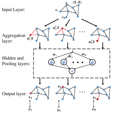
The output of the node of the GNN is
| (1) |
where is the activation function. We consider both regression and binary classification in this paper. For regression, is the ReLU function222Our result can be extended to the sigmoid activation function with minor changes. , and . For binary classification, we consider the sigmoid activation function where . Then is a binary variable generated from by , and .
Given , , and for all , the learning objective is to estimate , which is assumed to have a zero generalization error. The training objective is to minimize the empirical risk function,
| (2) |
where is the loss function. For regression, we use the squared loss function , and (2) is written as
| (3) |
For classification, we use the cross entropy loss function, and (2) is written as
| (4) |
Both (3) and (4) are nonconvex due to the nonlinear function . Moreover, while is a global minimum of (3), is not necessarily a global minimum of (4)333 is a global minimum if replacing all with in (4), but ’s are unknown in practice. . Furthermore, compared with NNs, the additional difficulty of analyzing the generalization performance of GNNs lies in the fact that each label is correlated with all the input features that are connected to node , as shown in the risk functions in (3) and (4).
Note that our model with is equivalent to the one-hidden-layer convolutional network (GCN) (Kipf & Welling, 2017) for binary classification. To study the multi-class classification problem, the GCN model in (Kipf & Welling, 2017) has nodes for classes in the second layer and employs the softmax activation function at the output. Here, our model has a pooling layer and uses the sigmoid function for binary classification. Moreover, we consider both regression and binary classification problems using the same model architecture with different activation functions. We consider one-hidden-layer networks following the state-of-art works in NNs (Du et al., 2018, 2017; Brutzkus & Globerson, 2017; Zhong et al., 2017b, a; Fu et al., 2018) and GNNs (Du et al., 2019; Verma & Zhang, 2019) because the theoretical analyses are extremely complex and still being developed for multiple hidden layers.
3 Proposed Learning Algorithm
In what follows, we illustrate the algorithm used for solving problems (3) and (4), summarized in Algorithm 1. Algorithm 1 has two components: a) accelerated gradient descent and b) tensor initialization. We initialize using the tensor initialization method (Zhong et al., 2017b) with minor modification for GNNs and update iterates by the Heavy Ball method (Polyak, 1987).
Accelerated gradient descent. Compared with the vanilla GD method, each iterate in the Heavy Ball method is updated along the combined directions of both the gradient and the moving direction of the previous iterates. Specifically, one computes the difference of the estimates in the previous two iterations, and the difference is scaled by a constant . This additional momentum term is added to the gradient descent update. When is , AGD reduces to GD.
During each iteration, a fresh subset of data is applied to estimate the gradient. The assumption of disjoint subsets is standard to simplify the analysis (Zhong et al., 2017a, b) but not necessary in numerical experiments.
Tensor initialization. The main idea of the tensor initialization method (Zhong et al., 2017b) is to utilize the homogeneous property of an activation function such as ReLU to estimate the magnitude and direction separately for each with . A non-homogeneous function can be approximated by piece-wise linear functions, if the function is strictly monotone with lower-bounded derivatives (Fu et al., 2018), like the sigmoid function. Our initialization is similar to those in (Zhong et al., 2017b; Fu et al., 2018) for NNs with some definitions are changed to handle the graph structure, and the initialization process is summarized in Subroutine 1.
Specifically, following (Zhong et al., 2017b), we define a special outer product, denoted by , such that for any vector and ,
| (5) |
where is the outer product and is the -th column of . Next, we define 444 stands for the expectation over the distribution of random variable .
| (6) |
| (7) |
| (8) |
where . The tensor is used to identify the directions of . depends on both the magnitudes and directions of . We will sequentially estimate the directions and magnitudes of from and . The matrix is used to identify the subspace spanned by . We will project to this subspace to reduce the computational complexity of decomposing .
Specifically, the values of , and are all estimated through samples, and let , , denote the corresponding estimates of these high-order momentum. Tensor decomposition method (Kuleshov et al., 2015) provides the estimates of the vectors from , and the estimates are denoted as .
However, the computation complexity of estimate through depends on poly(). To reduce the computational complexity of tensor decomposition, is in fact first projected to a lower-dimensional tensor (Zhong et al., 2017b) through a matrix . is the estimation of matrix and can be computed from the right singular vectors of . The column vectors of form a basis for the subspace spanned by , which indicates that for any . Then, from (8), is defined as
| (9) |
Similar to the case of , by applying the tensor decomposition method in , one can obtain a series of normalized vectors, denoted as , which are the estimates of . Then, is an estimate of since lies in the column space of with .
4 Main Theoretical Results
Theorems 1 and 2 state our major results about the GNN model for regression and binary classification, respectively. Before formally presenting the results, we first summarize the key findings as follows.
1. Zero generalization error of the learned model. Algorithm 1 can return exactly for regression (see (14)) and approximately for binary classification (see (19)). Specifically, since is often not a solution to (4), Algorithm 1 returns a critical point that is sufficiently close to , and the distance decreases with respect to the number of samples in the order of . Thus, with a sufficient number of samples, will be close to and achieves a zero generalization error approximately for binary classification. Algorithm 1 always returns exactly for regression, a zero generalization error is thus achieved.
2. Fast linear convergence of Algorithm 1. Algorithm 1 is proved to converge linearly to for regression and for classification, as shown in (14) and (18). That means the distance of the estimate during the iterations to (or ) decays exponentially. Moreover, Algorithm 1 converges faster than the vanilla GD. The rate of convergence is for regression 555 means that if for some constant , holds when is sufficiently large. means that for some constants and , holds when is sufficiently large. and for classification, where is the number of filters in the hidden layer. In comparison, the convergence rates of GD are and , respectively. Note that a smaller value of the rate of convergence corresponds to faster convergence. We remark that this is the first theoretical guarantee of AGD methods for learning GNNs.
3. Sample complexity analysis. can be estimated exactly for regression and approximately for classification, provided that the number of samples is in the order of , as shown in (13) and (17), where is the desired estimation error tolerance. has parameters, where is the number of nodes in the hidden layer, and is the feature dimension. Our sample complexity is order-wise optimal with respect to and only logarithmic with respect to the total number of features . We further show that the sample complexity is also positively associated with and . That characterizes the relationship between the sample complexity and graph structural properties. From Lemma 1, we know that given , is positively correlated with the average node degree . Thus, the required number of samples increases when the maximum and average degrees of the graph increase. That coincides with the intuition that more edges in the graph corresponds to the stronger dependence of the labels on neighboring features, thus requiring more samples to learn these dependencies. Our sample complexity quantifies this intuition explicitly.
Note that the graph structure affects this bound only through and . Different graph structures may require a similar number of samples to estimate , as long as they have similar and . We will verify this property on different graphs numerically in Figure 7.
Lemma 1.
Give an un-directed graph and the normalized adjacency matrix as defined in Section 2, the largest singular value of satisfies
| (12) |
where and are the average and maximum node degree, respectively.
4.1 Formal theoretical guarantees
To formally present the results, some parameters in the results are defined as follows. () is the -th singular value of . is the conditional number of . is defined as . For a fixed , both and can be viewed as constants and do not affect the order-wise analysis.
Theorem 1.
(Regression) Let be the sequence generated by Algorithm 1 to solve (3) with . Suppose the number of samples satisfies
| (13) |
for some constants and . Then converges linearly to with probability at least as
| (14) |
where is the rate of convergence that depends on . Moreover, we have
| (15) |
Specifically, let , we have
| (16) |
Theorem 2.
(Classification) Let be the sequence generated by Algorithm 1 to solve (4) with . Suppose the number of samples satisfies
| (17) |
for some positive constants and . Then, let be the nearest critical point of (4) to , we have that converges linearly to with probability at least as
| (18) |
The distance between and is bounded by
| (19) |
where is the rate of convergence that depends on , and is some positive constant. Moreover, we have
| (20) |
Specifically, let , we have
| (21) |
4.2 Comparison with existing works
Only (Verma & Zhang, 2019; Du et al., 2019) analyze the generalization error of one-hidden-layer GNNs in regression problems, while there is no existing work about the generalization error in classification problems. (Verma & Zhang, 2019; Du et al., 2019) show that the difference between the risks in the testing data and the training data decreases in the order of as the sample size increases. The GNN model in (Verma & Zhang, 2019) only has one filter in the hidden layer, i.e., , and the loss function is required to be a smooth function, excluding ReLU. Ref. (Du et al., 2019) only considers infinitely wide GNNs. In contrast, returned by Algorithm1 can achieve zero risks for both training data and testing data in regression problems. Our results apply to an arbitrary number of filters and the ReLU activation function. Moreover, this paper is the first work that characterizes the generalization error of GNNs for binary classification.
When is zero, our model reduces to one-hidden-layer NNs, and the corresponding sample complexity is . Our results are at least comparable to, if not better than, the state-of-art theoretical guarantees that from the prespective of model estimation for NNs. For example, (Zhong et al., 2017b) considers one-hidden-layer NNs for regression and proves the linear convergence of their algorithm to the ground-truth model parameters. The sample complexity of (Zhong et al., 2017b) is also linear in , but the activation function must be smooth. (Zhang et al., 2019) considers one-hidden-layer NNs with the ReLU activation function for regression, but the algorithm cannot converge to the ground-truth parameters exactly but up to a statistical error. Our result in Theorem 1 applies to the nonsmooth ReLU function and can recover exactly. (Fu et al., 2018) considers one-hidden-layer NNs for classification and proves linear convergence of their algorithm to a critical point sufficiently close to with the distance bounded by . The convergence rate in (Fu et al., 2018) is , while Algorithm 1 has a faster convergence rate of .
5 Numerical Results
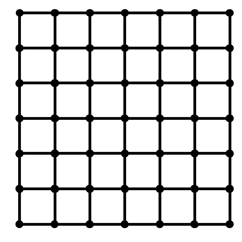
We verify our results on synthetic graph-structured data. We consider four types of graph structures as shown in Figure 2: (a) a connected-cycle graph having each node connecting to its closet neighbors; (b) a two-dimensional grid having each node connecting to its nearest neighbors in axis-aligned directions; (c) a random -regular graph having each node connecting to other nodes randomly; (d) a random graph with bounded degree having each node degree selected from with probability and with probability for some .



The feature vectors are randomly generated from the standard Gaussian distribution . Each entry of is generated from independently. are computed based on (1). The labels are generated by and for regression and classification problems, respectively.
During each iteration of Algorithm 1, we use the whole training data to calculate the gradient. The initialization is randomly selected from to reduce the computation. As shown in (Fu et al., 2018; Zhang et al., 2019), the random initialization and the tensor initialization have very similar numerical performance. We consider the learning algorithm to be successful in estimation if the relative error, defined as , is less than , where is the weight matrix returned by Algorithm 1 when it terminates.
5.1 Convergence rate
We first verify the linear convergence of Algorithm 1, as shown in (14) and (18). Figure 3 (a) and (b) show the convergence rate of Algorithm 1 when varying the number of nodes in the hidden layer . The dimension of the feature vectors is chosen as , and the sample size is chosen as . We consider the connected-cycle graph in Figure 2 (a) with . All cases converge to with the exponential decay. Moreover, from Figure 3, we can also see that the rate of convergence is almost a linear function of . That verifies our theoretical result of the convergence rate of in (16).
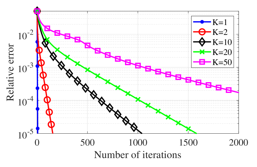
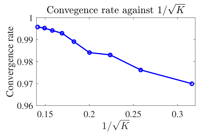
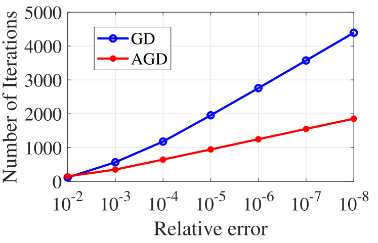
Figure 4 compares the rates of convergence of AGD and GD in regression problems. We consider a connected-cycle graph with . The number of samples , , and . Starting with the same initialization, we show the smallest number of iterations needed to reach a certain estimation error, and the results are averaged over independent trials. Both AGD and GD converge linearly. AGD requires a smaller number of the iterations than GD to achieve the same relative error.
5.2 Sample complexity
We next study the influence of , , , and different graph structures on the estimation performance of Algorithm 1. These relationships are summarized in the sample complexity analyses in (13) and (17) of section 4.1. We have similar numerical results for both regression and classification, and here we only present the regression case.
Figures 5 (a) and (b) show the successful estimation rates when the degree of graph and the feature dimension changes. We consider the connected-cycle graph in Figure 2 (a), and is kept as 5. is in Figure 5 (a), and is in Figure 5 (b). The results are averaged over independent trials. White block means all trials are successful while black block means all trials fail. We can see that the required number of samples for successful estimation increases as and increases.
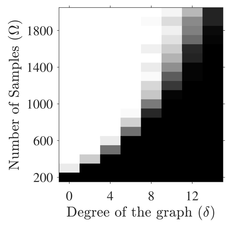
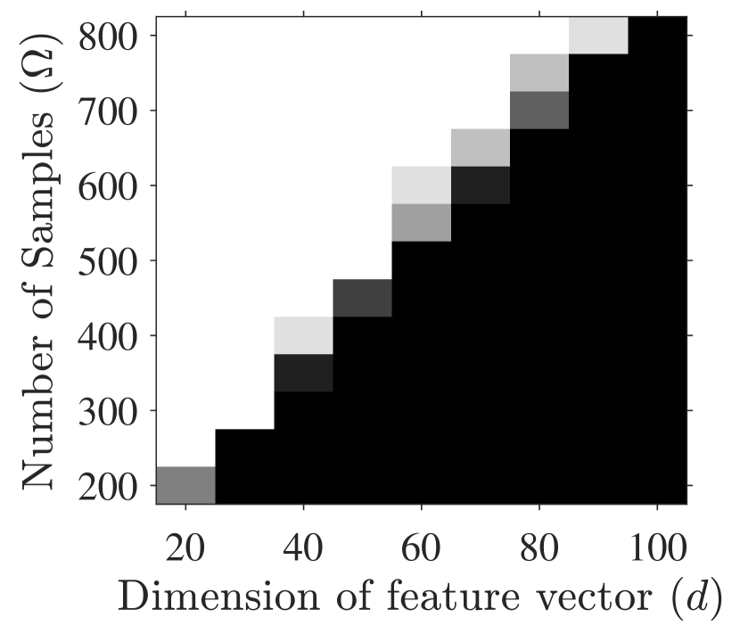
Figure 6 shows the success rate against the sample size for the random graph in Figure 2(d) with different average node degrees. We vary to change the average node degree . and are fixed as and , respectively. The successful rate is calculated based on independent trials. We can see that more samples are needed for successful recovery for a larger when the maximum degree is fixed.
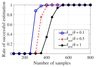
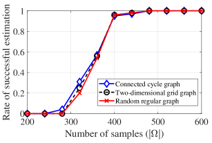
Figure 7 shows the success rate against for three different graph structures, including a connected cycle, a two-dimensional grid, and a random regular graph in Figure 2 (a), (b), and (c). The maximum degrees of these graphs are all fixed with . The average degrees of the connected-circle and the random -regular graphs are also . is very close to for the two-dimensional grid when the graph size is large enough, because only the boundary nodes have smaller degrees, and the percentage of boundary nodes decays as the graph size increases. Then from Lemma 1, we have is for all these graphs. Although these graphs have different structures, the required numbers of samples to estimate accurately are the same, because both and are the same. One can verify this property from Figure 7 where all three curves almost coincide.
5.3 Accuracy in learning
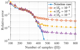
We study the learning accuracy of , characterized in (14) for regression and (19) for classification. For regression problems, we simulate the general cases when the labels are noisy, i.e., . The noise are i.i.d. from , and the noise level is measured by , where is the average energy of the noiseless labels , calculated as . The number of hidden nodes is 5, and the dimension of each feature is as . We consider a connected-circle graph with . Figure 8 shows the performance of Algorithm 1 in the noisy case. We can see that when the number of samples exceeds , which is the degree of freedom of , the relative error decreases dramatically. Also, as increases, the relative error converges to the noise level. When there is no noise, the estimation of is accurate.
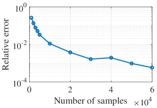
For binary classification problems, Algorithm 1 returns the nearest critical point to . We show the distance between the returned model and the ground-truth model against the number of samples in Figure 9. We consider a connected-cycle graph with the degree . and . The relative error is averaged over independent trials. We can see that the distance between the returned model and the ground-truth model indeed decreases as the number of samples increases.
6 Conclusion
Despite the practical success of graph neural networks in learning graph-structured data, the theoretical guarantee of the generalizability of graph neural networks is still elusive. Assuming the existence of a ground-truth model, this paper shows theoretically, for the first time, learning a one-hidden-layer graph neural network with a generation error that is zero for regression or approximately zero for binary classification. With the tensor initialization, we prove that the accelerated gradient descent method converges to the ground-truth model exactly for regression or approximately for binary classification at a linear rate. We also characterize the required number of training samples as a function of the feature dimension, the model size, and the graph structural properties. One future direction is to extend the analysis to multi-hidden-layer neural networks.
7 Acknowledge
This work was supported by AFOSR FA9550-20-1-0122 and the Rensselaer-IBM AI Research Collaboration (http://airc.rpi.edu), part of the IBM AI Horizons Network (http://ibm.biz/AIHorizons).
References
- Battaglia et al. (2016) Battaglia, P., Pascanu, R., Lai, M., Rezende, D. J., et al. Interaction networks for learning about objects, relations and physics. In Advances in neural information processing systems, pp. 4502–4510, 2016.
- Brutzkus & Globerson (2017) Brutzkus, A. and Globerson, A. Globally optimal gradient descent for a convnet with gaussian inputs. In Proceedings of the 34th International Conference on Machine Learning-Volume 70, pp. 605–614. JMLR. org, 2017.
- Cao & Gu (2020) Cao, Y. and Gu, Q. Generalization error bounds of gradient descent for learning overparameterized deep relu networks. 2020.
- Chizat & Bach (2018) Chizat, L. and Bach, F. A note on lazy training in supervised differentiable programming. arXiv preprint arXiv:1812.07956, 8, 2018.
- Du et al. (2017) Du, S. S., Lee, J. D., and Tian, Y. When is a convolutional filter easy to learn? arXiv preprint, http://arxiv.org/abs/1709.06129, 2017.
- Du et al. (2018) Du, S. S., Lee, J. D., Tian, Y., Singh, A., and Poczos, B. Gradient descent learns one-hidden-layer cnn: Don’t be afraid of spurious local minima. In International Conference on Machine Learning, pp. 1338–1347, 2018.
- Du et al. (2019) Du, S. S., Hou, K., Salakhutdinov, R. R., Poczos, B., Wang, R., and Xu, K. Graph neural tangent kernel: Fusing graph neural networks with graph kernels. In Advances in Neural Information Processing Systems, pp. 5724–5734, 2019.
- Duvenaud et al. (2015) Duvenaud, D. K., Maclaurin, D., Iparraguirre, J., Bombarell, R., Hirzel, T., Aspuru-Guzik, A., and Adams, R. P. Convolutional networks on graphs for learning molecular fingerprints. In Advances in neural information processing systems, pp. 2224–2232, 2015.
- Fu et al. (2018) Fu, H., Chi, Y., and Liang, Y. Guaranteed recovery of one-hidden-layer neural networks via cross entropy. arXiv preprint arXiv:1802.06463, 2018.
- Ge et al. (2018) Ge, R., Lee, J. D., and Ma, T. Learning one-hidden-layer neural networks with landscape design. In International Conference on Learning Representations, 2018. URL https://openreview.net/forum?id=BkwHObbRZ.
- Gilbert et al. (2005) Gilbert, A. C., Muthukrishnan, S., and Strauss, M. Improved time bounds for near-optimal sparse fourier representation via sampling. In Proc. SPIE, 2005.
- Gilmer et al. (2017) Gilmer, J., Schoenholz, S. S., Riley, P. F., Vinyals, O., and Dahl, G. E. Neural message passing for quantum chemistry. In Proceedings of the 34th International Conference on Machine Learning-Volume 70, pp. 1263–1272. JMLR. org, 2017.
- Hamilton et al. (2017) Hamilton, W., Ying, Z., and Leskovec, J. Inductive representation learning on large graphs. In Advances in neural information processing systems, pp. 1024–1034, 2017.
- Jacot et al. (2018) Jacot, A., Gabriel, F., and Hongler, C. Neural tangent kernel: Convergence and generalization in neural networks. In Advances in neural information processing systems, pp. 8571–8580, 2018.
- Janson (2004) Janson, S. Large deviations for sums of partly dependent random variables. Random Structures & Algorithms, 24(3):234–248, 2004.
- Kipf & Welling (2017) Kipf, T. N. and Welling, M. Semi-supervised classification with graph convolutional networks. In Proc. International Conference on Learning (ICLR), 2017.
- Kuleshov et al. (2015) Kuleshov, V., Chaganty, A., and Liang, P. Tensor factorization via matrix factorization. In Artificial Intelligence and Statistics, pp. 507–516, 2015.
- Li et al. (2016) Li, Y., Tarlow, D., Brockschmidt, M., and Zemel, R. Gated graph sequence neural networks. International Conference on Learning Representations (ICLR), 2016.
- Monfardini et al. (2006) Monfardini, G., Di Massa, V., Scarselli, F., and Gori, M. Graph neural networks for object localization. Frontiers in Artificial Intelligence and Applications, 141:665, 2006.
- Morris et al. (2019) Morris, C., Ritzert, M., Fey, M., Hamilton, W. L., Lenssen, J. E., Rattan, G., and Grohe, M. Weisfeiler and leman go neural: Higher-order graph neural networks. In Proceedings of the AAAI Conference on Artificial Intelligence, volume 33, pp. 4602–4609, 2019.
- Nitanda & Suzuki (2019) Nitanda, A. and Suzuki, T. Refined generalization analysis of gradient descent for over-parameterized two-layer neural networks with smooth activations on classification problems. arXiv preprint arXiv:1905.09870, 2019.
- Polyak (1987) Polyak, B. T. Introduction to optimization. New York: Optimization Software, Inc, 1987.
- Safran & Shamir (2018) Safran, I. and Shamir, O. Spurious local minima are common in two-layer relu neural networks. In International Conference on Machine Learning, pp. 4430–4438, 2018.
- Scarselli et al. (2008) Scarselli, F., Gori, M., Tsoi, A. C., Hagenbuchner, M., and Monfardini, G. The graph neural network model. IEEE Transactions on Neural Networks, 20(1):61–80, 2008.
- Shamir (2018) Shamir, O. Distribution-specific hardness of learning neural networks. The Journal of Machine Learning Research, 19(1):1135–1163, 2018.
- Veličković et al. (2018) Veličković, P., Cucurull, G., Casanova, A., Romero, A., Lio, P., and Bengio, Y. Graph attention networks. International Conference on Learning Representations (ICLR), 2018.
- Verma & Zhang (2019) Verma, S. and Zhang, Z.-L. Stability and generalization of graph convolutional neural networks. In Proceedings of the 25th ACM SIGKDD International Conference on Knowledge Discovery & Data Mining, pp. 1539–1548, 2019.
- Vershynin (2010) Vershynin, R. Introduction to the non-asymptotic analysis of random matrices. arXiv preprint arXiv:1011.3027, 2010.
- Wu et al. (2019) Wu, F., Souza, A., Zhang, T., Fifty, C., Yu, T., and Weinberger, K. Simplifying graph convolutional networks. In International Conference on Machine Learning, pp. 6861–6871, 2019.
- Xu et al. (2018) Xu, K., Li, C., Tian, Y., Sonobe, T., Kawarabayashi, K.-i., and Jegelka, S. Representation learning on graphs with jumping knowledge networks. In International Conference on Machine Learning, pp. 5453–5462, 2018.
- Xu et al. (2019) Xu, K., Hu, W., Leskovec, J., and Jegelka, S. How powerful are graph neural networks? International Conference on Learning Representations (ICLR), 2019.
- Ying et al. (2018) Ying, R., He, R., Chen, K., Eksombatchai, P., Hamilton, W. L., and Leskovec, J. Graph convolutional neural networks for web-scale recommender systems. In Proceedings of the 24th ACM SIGKDD International Conference on Knowledge Discovery & Data Mining, pp. 974–983, 2018.
- Zhang et al. (2019) Zhang, X., Yu, Y., Wang, L., and Gu, Q. Learning one-hidden-layer relu networks via gradient descent. In The 22nd International Conference on Artificial Intelligence and Statistics, pp. 1524–1534, 2019.
- Zhong et al. (2017a) Zhong, K., Song, Z., and Dhillon, I. S. Learning non-overlapping convolutional neural networks with multiple kernels. arXiv preprint arXiv:1711.03440, 2017a.
- Zhong et al. (2017b) Zhong, K., Song, Z., Jain, P., Bartlett, P. L., and Dhillon, I. S. Recovery guarantees for one-hidden-layer neural networks. In Proceedings of the 34th International Conference on Machine Learning-Volume 70, pp. 4140–4149. JMLR. org, https://arxiv.org/abs/1706.03175, 2017b.
- Zhong et al. (2017c) Zhong, K., Song, Z., Jain, P., Bartlett, P. L., and Dhillon, I. S. Recovery guarantees for one-hidden-layer neural networks. arXiv preprint, http://arxiv.org/abs/1706.03175, 2017c.
Appendix A Proof of Theorem 1
In this section, before presenting the proof of Theorem 1, we start with defining some useful notations. Recall that in (3), the empirical risk function for linear regression problem is defined as
| (22) |
Population risk function, which is the expectation of the empirical risk function, is defined as
| (23) |
Then, the road-map of the proof can be summarized in the following three steps.
First, we show the Hessian matrix of the population risk function is positive-definite at ground-truth parameters and then characterize the local convexity region of near , which is summarized in Lemma 2.
Second, is non-smooth because of ReLU activation, but is smooth. Hence, we characterize the gradient descent term as . During this step, we need to apply concentration theorem to bound to its expectation , which is summarized in Lemma 3.
Third, we take the momentum term of into consideration and obtain the following recursive rule:
| (24) |
Then, we know iterates converge to the ground-truth with a linear rate which is the largest singlar value of matrix . Recall that AGD reduces to GD with , so our analysis applies to GD method as well. We are able to show the convergence rate of AGD is faster than GD by proving the largest singluar value of is smaller than for some . Lemma 4 provides the estimation error of and sample complexity to guarantee is less than for .
Lemma 2.
Let be the population risk function in (23) for regression problems, then for any that satisfies
| (25) |
the second-order derivative of is bounded as
| (26) |
Lemma 3.
Lemma 4.
Assume the number of samples , the tensor initialization method via Subroutine 1 outputs such that
| (28) |
with probability at least .
The proofs of Lemmas 2 and 3 are included in Appendix A.1 and A.2, respectively, while the proof of Lemma 4 can be found in Appendix D. With these three preliminary lemmas on hand, the proof of Theorem 1 is formally summarized in the following contents.
Proof of Theorem 1.
The update rule of is
| (29) |
Since is a smooth function, by the intermediate value theorem, we have
| (30) |
where lies in the convex hull of and .
Let be the eigen-decomposition of . Then, we define
| (34) |
Since , we know and share the same eigenvalues. Let be the -th eigenvalue of , then the corresponding -th eigenvalue of , denoted by , satisfies
| (35) |
Then, we have
| (36) |
and
| (37) |
Note that the other root of (35) is abandoned because the root in (36) is always no less than the other root with . By simple calculations, we have
| (38) |
Moreover, achieves the minimum when .
Let us first assume satisfies (25), then from Lemma 2, we know that
Let and . If we choose such that
| (39) |
then we have and for any .
Let , then equals to . Then, for any , we have
| (40) |
Then, let
| (41) |
we need . Combining (40) and (41), we have
| (42) |
Let , we have
if .
Hence, with and , we have
| (43) |
provided satisfies (25), and
| (44) |
Then, we can start mathematical induction of (43) over .
Base case: According to Lemma 4, we know that (25) holds for if
| (45) |
According to Theorem 1, it is clear that the number of samples satisfies (45), then (25) indeed holds for . Since (25) holds for and in Theorem 1 satisfies (44) as well, we have (43) holds for .
Induction step: Assuming (43) holds for , we need to show that (43) holds for . That is to say, we need satisfies (44), which holds naturally from Theorem 1.
Therefore, when , we know that (43) holds for all with probability at least . By simple calculations, we can obtain
| (46) |
∎
A.1 Proof of Lemma 2
In this section, we provide the proof of Lemma 2 which shows the local convexity of in a small neighborhood of . The roadmap is to first bound the smallest eigenvalue of in the ground truth as shown in Lemma 5, then show that the difference of between any fixed point in this region and the ground truth is bounded in terms of by Lemma 6.
Lemma 5.
The second-order derivative of at the ground truth satisfies
| (47) |
Lemma 6.
Suppose satisfies (25), we have
| (48) |
A.2 Proof of Lemma 3
The proof of Lemma 3 is mainly to bound the concentration error of random variables as shown in (60). We first show that is a sub-exponential random variable, and the definitions of sub-Gaussian and sub-exponential random variables are provided in Definitions 1 and 2. Though Hoeffding’s inequality provides the concentration error for sum of independent random variables, random variables with different are not independent. Hence, we introduce Lemma 7 to provide the upper bound for the moment generation function of the sum of partly dependent random variables and then apply standard Chernoff inequality. Lemmas 8 and 9 are standard tools in analyzing spectral norms of high-demensional random matrices.
Definition 1 (Definition 5.7, (Vershynin, 2010)).
A random variable is called a sub-Gaussian random variable if it satisfies
| (50) |
for all and some constant . In addition, we have
| (51) |
for all and some constant , where is the sub-Gaussian norm of defined as .
Moreover, a random vector belongs to the sub-Gaussian distribution if one-dimensional marginal is sub-Gaussian for any , and the sub-Gaussian norm of is defined as .
Definition 2 (Definition 5.13, (Vershynin, 2010)).
A random variable is called a sub-exponential random variable if it satisfies
| (52) |
for all and some constant . In addition, we have
| (53) |
for and some constant , where is the sub-exponential norm of defined as .
Lemma 7.
Given a sampling set that contains partly dependent random variables, for each , suppose is dependent with at most random variables in (including itself), and the moment generate function of satisfies for some constant that may depend on . Then, the moment generation function of is bounded as
| (54) |
Lemma 8 (Lemma 5.2, (Vershynin, 2010)).
Let denote a unit ball in . Then, a subset is called a -net of if every point can be approximated to within by some point , i.e. . Then the minimal cardinality of a -net satisfies
| (55) |
Lemma 9 (Lemma 5.3, (Vershynin, 2010)).
Let be an matrix, and let be a -net of in for some . Then
| (56) |
The proof of Lemma 7 can be found in Appendex A.3. With these preliminary Lemmas and definition on hand, the proof of Lemma 3 is formally summarized in the following contents.
Proof of Lemma 3 .
We have
| (57) |
and
| (58) |
The gradients of are
| (59) |
Let us define
| (60) |
then for any normalized , we have
| (61) |
where the first inequality comes from the Cauchy-Schwarz inequality. Furthermore, belongs to the Gaussian distribution and thus is a sub-Gaussian random vector as well. Then, from Definition 1, we have
| (62) |
Then, we have
| (63) |
Therefore, from Definition 2, belongs to the sub-exponential distribution with
| (64) |
Recall that each node is connected with at most other nodes. Hence, for any fixed , there are at most (including itself) elements in are dependant with . From Lemma 7, the moment generation function of satisfies
| (65) |
By Chernoff inequality, we have
| (66) |
for any .
Let and , we have
| (67) |
with probability at least .
A.3 Proof of auxiliary lemmas for regression problems
A.3.1 Proof of Lemma 5
A.3.2 Proof of Lemma 6
Proof of Lemma 6 .
The second-order derivative of is written as
| (71) |
For any normalized , we have
| (72) |
It is easy to verify there exists a basis such that with spanning a subspace that contains and . Then, for any , we have a unique such that
Also, since , we have . Then, we have
where and is the probability density function of . Next, we consider spherical coordinates with . Hence,
| (73) |
It is easy to verify that only depends on the direction of and
only depends on . Then, we have
| (74) |
Define a set . If , then and have different signs, which means the value of and are different. This is equivalent to say that
| (75) |
Moreover, if , then we have
| (76) |
Define a set such that
| (77) |
Hence, we have that
| (78) |
Since , belongs to the uniform distribution on , we have
| (79) |
Hence, (81) and (79) suggest that
| (80) |
Then, we have
| (81) |
All in all, we have
| (82) |
∎
A.3.3 Proof of Lemma 7
Proof of Lemma 7 .
According to the Definitions in (Janson, 2004), there exists a family of , where and , such that , and by equations (2.1) and (2.2) in (Janson, 2004). Then, let be any positive numbers with . By Jensen’s inequality, for any , we have
| (83) |
where .
Then, we have
| (84) |
Let , then we have
| (85) |
By Cauchy-Schwarz inequality, we have
| (86) |
Hence, we have
| (87) |
∎
Appendix B Proof of Theorem 2
Recall that the empirical risk function in (4) is defined as
| (88) |
The population risk function is defined as
| (89) |
The road-map of proof for Theorem 2 follows the similar three steps as those for Theorem 1. The major differences lie in three aspects: (i) in the second step, the objective function is smooth since the activation function is sigmoid. Hence, we can directly apply the mean value theorem as to characterize the effects of the gradient descent term in each iteration, and the error bound of is provided in Lemma 10; (ii) the objective function is the sum of cross-entry loss functions, which have more complex structure of derivatives than those of square loss functions; (iii) as the convergent point may not be the critical point of empirical loss function, we need to provide the distance from the convergent point to the ground-truth parameters additionally, where Lemma 11 is used.
Lemmas 10 and 11 are summarized in the following contents. Also, the notations and follow the same definitions as in (27). The proofs of Lemmas 10 and 11 can be found in Appendix B.1 and B.2, respectively.
Lemma 10.
For any that satisfies
| (90) |
then the second-order derivative of the empirical risk function in (88) for binary classification problems is bounded as
| (91) |
provided the number of samples satisfies
| (92) |
Lemma 11.
With these preliminary lemmas, the proof of Theorem 2 is formally summarized in the following contents.
Proof of Theorem 2.
The update rule of is
| (94) |
Since is a critical point, then we have . By the intermediate value theorem, we have
| (95) |
where lies in the convex hull of and .
Next, we have
| (96) |
Let , so we have
Then, we have
| (97) |
Let be the -th eigenvalue of , and be the -th eigenvalue of matrix . Following the similar analysis in proof of Theorem 1, we have
| (98) |
Moreover, achieves the minimum when .
Let us first assume satisfies (90) and the number of samples satisfies (92), then from Lemma 10, we know that
We define and . Also, for any , we have
| (99) |
Let , we have
Hence, with probability at least , we have
| (100) |
provided that satisfies (25), and
| (101) |
According to Lemma 4, we know that (90) holds for if
| (102) |
Finally, by the mean value theorem, we have
| (103) |
for some between and . Since is the local minima, we have . That is to say
| (104) |
which implies
| (105) |
From Lemma 10, we know that
| (106) |
From Lemma 11, we know that
| (107) |
Plugging inequalities (106) and (107) back into (105), we have
| (108) |
∎
B.1 Proof of Lemma 10
The roadmap of proof for Lemma 10 follows the similar steps as those of Lemma 2 for regression problems. Lemmas 12, 13 and 14 are the preliminary lemmas, and their proofs can be found in Appendix B.2. The proof of Lemma 10 is summarized after these preliminary lemmas.
Lemma 12.
The second-order derivative of at the ground truth satisfies
| (109) |
Lemma 13.
Suppose is the population loss function with respect to binary classification problems, then we have
| (110) |
Lemma 14.
Suppose is the empirical loss function with respect to binary classification problems, then the second-order derivative of is close to its expectation with an upper bound as
| (111) |
with probability at least .
B.2 Proof of auxiliary lemmas for binary classification problems
B.2.1 Proof of Lemma 12
Proof of Lemma 12 .
Since , then we have
| (117) |
for any .
Then, for any with , the lower bound can be obtained from
| (118) |
Also, for the upper bound, we have
| (119) |
For the denominator item, we have
| (120) |
Hence, we have
| (121) |
∎
B.2.2 Proof of Lemma 13
B.2.3 Proof of Lemma 14
Proof of Lemma 14 .
Recall that
| (129) |
and
| (130) |
When and , we have
| (131) |
and
| (132) |
When and , we have
| (133) |
and
| (134) |
Similar to (132) and (134), we can obtain the following inequality for .
| (135) |
Then, for any , we have
| (136) |
Next, we show that belongs to the sub-exponential distribution. For any , we have
| (137) |
Hence, belongs to the sub-exponential distribution with . Then, the moment generation function of can be bounded as
| (138) |
for some positive constant and any . From Lemma 7 and Chernoff bound, we have
| (139) |
with probability at least . By selecting in Lemmas 8 and 9, we have
| (140) |
with probability at least .
In conclusion, we have
| (141) |
with probability at least . ∎
B.2.4 Proof of Lemma 11
Proof of Lemma 11.
Recall that the first-order derivative of is calculated from
| (142) |
Similar to (134), we have
| (143) |
Similar to (137), for any fixed , we can show that random variable belongs to sub-exponential distribution with the same bounded norm up to a constant. Hence, by applying Lemma 7 and the Chernoff bound, we have
| (144) |
with probability at least . ∎
Appendix C Proof of Lemma 1
Proof of Lemma 1.
Let denote the adjacency matrix, then we have
| (145) |
where denotes the degree of node . Let be the eigenvetor of the maximum eigenvalue . Since and is diagonal matrix, then is the eigenvector to as well. Then, let be the index of the largest value of vector as , we have
| (146) |
where is the -th row of .
Since is a diagonal matrix with , then we can conclude the inequality in this lemma. ∎
Appendix D Proof of Lemma 4
The proof of Lemma 4 is divided into three major parts to bound , and in (153). Lemmas 15, 16 and 17 provide the error bounds for , and , respectively. The proofs of these preliminary lemmas are similar to those of Theorem 5.6 in (Zhong et al., 2017b), the difference is to apply Lemma 7 plus Chernoff inequality instead of standard Hoeffding inequality, and we skip the details of the proofs of Lemmas 15, 16 and 17 here.
Lemma 15.
Suppose is defined as in (7) and is the estimation of by samples. Then, with probability , we have
| (147) |
provided that .
Lemma 16.
Let be generated by step 4 in Subroutine 1. Suppose is defined as in (9) and is the estimation of by samples. Further, we assume is an orthogonal basis of and satisfies . Then, provided that , with probability at least , we have
| (148) |
Lemma 17.
Suppose is defined as in (6) and is the estimation of by samples. Then, with probability , we have
| (149) |
provided that .
Lemma 18 ((Zhong et al., 2017b), Lemma E.6).
Let be an orthogonal basis of and be generated by step 4 in Subroutine 1. Assume . Then, for some small , we have
| (150) |
Lemma 19 ((Zhong et al., 2017b), Lemma E.13).
Proof of Lemma 4.
we have
| (153) |
From Lemma 18, we have
| (154) |
where the last inequality comes from Lemma 15. Then, from (7), we know that
| (155) |
From Theorem 3 in (Kuleshov et al., 2015), we have
| (156) |
To guarantee the condition (151) in Lemma 19 hold, according to Lemmas 15 and 16, we need . Then, from Lemma 19, we have
| (157) |
Since , according to Lemmas 15, 16 and 17, we have
| (158) |
provided . ∎