Local Convolutions Cause an Implicit Bias towards High Frequency Adversarial Examples
Abstract
Adversarial Attacks are still a significant challenge for neural networks. Recent efforts has shown that adversarial perturbations typically contain high-frequency features, but the root cause of this phenomenon remains unknown. Inspired by theoretical work on linear full-width convolutional models, we hypothesize that convolutional operations with localized kernels are implicitly biased to learn high frequency features, and that this is one of the root causes of high frequency adversarial examples. To test this hypothesis, we analyzed the impact of different choices of linear and nonlinear architectures on the implicit bias of the learned features and the adversarial perturbations, in spatial and frequency domains. We find that, independently of the training dataset, convolutional operations have higher frequency adversarial attacks compared to other architectural parametrizations, and this phenomenon is exacerbated with stronger locality of the convolutional kernels. The explanation for the kernel size dependence involves the Fourier Uncertainty Principle: a spatially-limited (local in the space domain) filter cannot also be frequency-limited (local in the frequency domain). Using larger convolution kernel sizes or avoiding convolutions (e.g. by using Vision Transformers or MLP-style architectures) significantly reduces this high frequency bias.
Looking forward, our work strongly suggests that understanding and controlling the implicit bias of architectures will be essential for achieving adversarial robustness.
1 Introduction
Despite the enormous progress in training neural networks to solve hard tasks, they remain surprisingly and stubbornly sensitive to imperceptibly small worst-case perturbations known as adversarial examples. There has been a significant amount of work regarding the nature and structure of adversarial examples [1, 2, 3, 4, 5, 6, 7, 8, 9]. One particular experimental observation is that, oftentimes, adversarial examples show a large amount of energy content in the high frequencies [10]. Furthermore, previous work has shown that adversarial examples are not just random perturbations of the input space but they contain dataset-specific information which is informative of class decision boundaries [9]. A natural question is then: does the concentration of energy in the high frequencies reflect some features of the task? Wang et al., 2020 showed that high frequency features are necessary for high generalization performance of different models trained on CIFAR10 [11]. They argue that learning these high frequency features is effectively a data-wise phenomenon, showing that models that use lower-frequency features had lower accuracy on CIFAR10. These results point out that the presence of high frequency features are conditioned to their usefulness in this dataset. Moreover, Maiya et al., 2021 provided evidence that different datasets produced adversarial examples with different concentration of energy in frequency domain which are related to the dataset statistics [12]. Furthermore, previous work has also shown that sensitivity to certain frequency based features can be altered by decreasing the reliability of those features in the dataset via data augmentations [13, 14, 15]. All together these results suggest that feature selection, and specifically high frequency features, are mainly driven by dataset statistics.
However, even though different datasets have different features that are correlated with the target function, there are usually more useful features than necessary for equal performance [9]. So why is any given model learning frequency based features and more specifically high frequency features? Different theories have been produced for understanding robustness and generalization of neural networks through a frequency lens. For example, Universal Adversarial Perturbations (UAPs) is a method to compute which directions in input space are neural networks sensitive to [16]. The authors of this work found that convolutional neural networks were sensitive to noise in the Fourier Basis, where other models such as MLPs are not so. Moreover the work about Neural Anisotropic Directions (NADs) found that neural networks use linearly separable directions for classification and these directions can be approximated by directions in the frequency domain [17, 18].
Here we take a different and more principled approach by relying on the concept of implicit bias to answer this question. The idea behind implicit bias is that the loss landscape of an overparameterized network has infinitely many global minima, and which global minimum one converges to after training depends on many factors, including the choice of model architecture and parametrization [19, 20], the initialization scheme [21] and the optimization algorithm [22, 23, 24]. The implicit bias of state-of-the-art models has been shown to play a critical role in the generalization of deep neural networks [25, 26]. Recent theoretical work [19] on -layer deep linear networks proved that (i) fully connected layers induce a depth-independent ridge () regularizer in the spatial domain of the networks weights whereas, surprisingly, full-width convolutional layers induce a depth-dependent sparsity () regularizer in the frequency domain. Linear full-width convolutional models are different from the high-performance convolutional neural networks (CNNs) used in practice. Nonetheless, we hypothesised that similar mechanisms might play a role for deep nonlinear models with local convolutions: the high frequency nature of commonly-found adversarial perturbations is due to the implicit bias induced by the specific architectural choice and not only by the dataset statistics. More formally, we propose the Implicit Fourier Regularization (IFR) hypothesis (see Figure 1):
Implicit regularization in frequency domain, directly caused by the translation invariance and spatially limited nature of bounded-width convolutions, yields a strong bias towards high frequency features and adversarial perturbations.
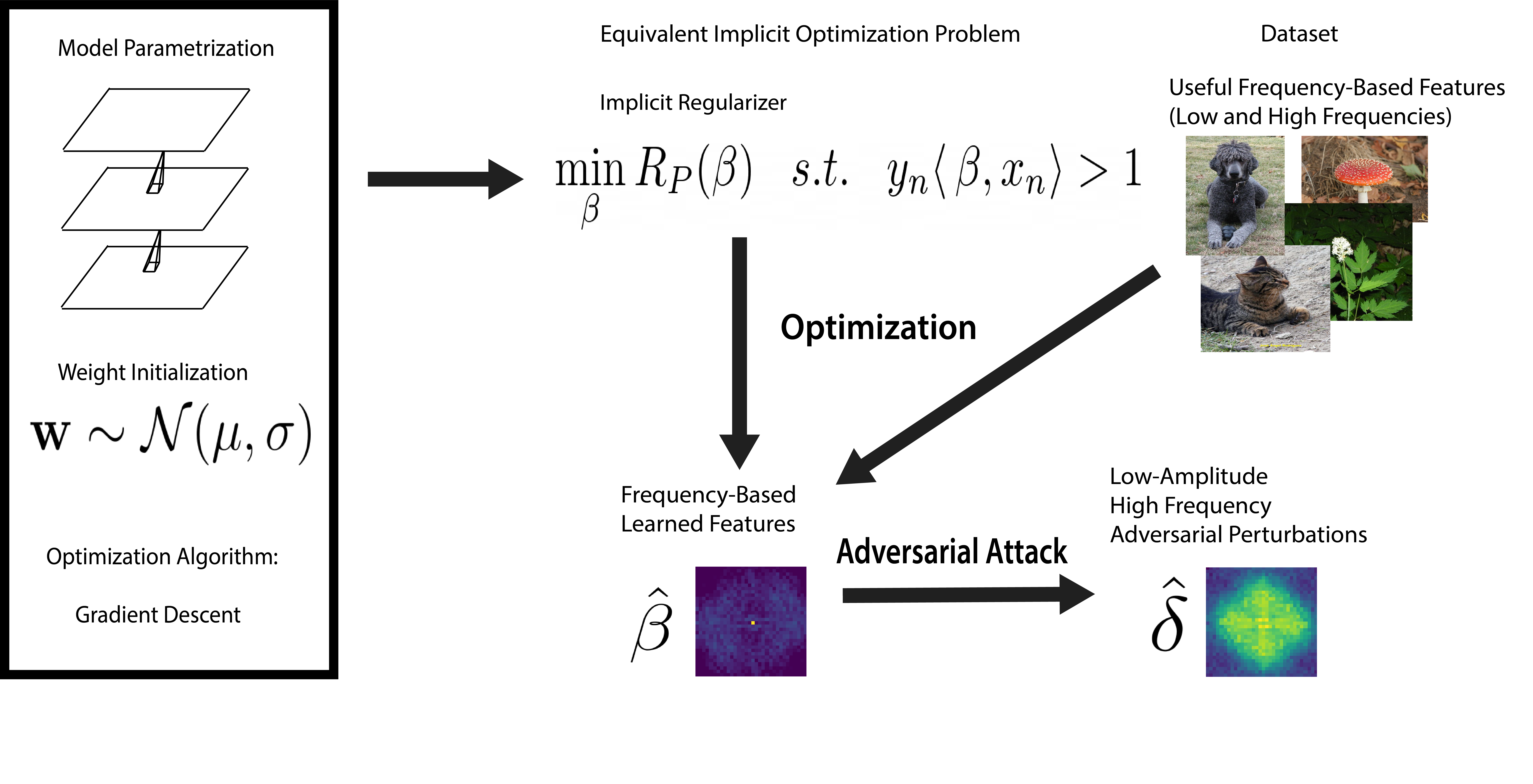
The IFR hypothesis suggests that if a datasets presents useful high frequency features, models with bounded-width convolutional parametrizations will be biased to learn these features. This is because local convolutions induce a specific implicit bias, encouraging the linear features to possess more energy in high frequencies which, in turn, induce high frequency adversarial perturbations. More broadly, our work establishes the relationship between the implicit regularization due to model parametrization and the structure of adversarial perturbations.
2 Experimental Results
In the following we are going to test different aspects of the IFR principle. In particular in section 2.1 we analyze and compare the Fourier spectrum of the weights and adversarial perturbations of full width architectures (convolutional or not, deep or not, linear or not, where the support of the weights is the full image). In section 2.2 we repeat the analysis for bounded width convolutional models and compare the spectral analysis with that of the full width models. Then, in section 2.3 and 2.5 we analyze how convolutional weights sharing impacts the Fourier spectrum of the weights and adversarial perturbations. In section 2.4 we further test the model spectral bias injecting explicitly frequency-targeted shortcuts in the dataset and analyze the different models performances. Finally in section 2.6 we test if the results obtained in the previous sections extends to a zoo complex models trained on Imagenet.
2.1 Confirming Gunasekar et al, 2018 [19] results and extension to full width non linear models. Relationship to adversarial perturbations.
To establish the relationship between implicit regularization and adversarial perturbations, we based our experiments on the recent theoretical work of Gunasekar et al., 2018 where the authors have shown that shallow linear convolutional neural networks ( full-width circular convolutional linear layers followed by one fully connected linear layer) induce an implicit sparsity-promoting regularizer in the Fourier domain. Specifically, the regularizer is: where is the Discrete Fourier Transform (DFT) of the end-to-end linear transformation represented by the Full Width Convolutional network (FWC) with weights and the number of layers [19]. The authors proved that different linear layer parametrizations induce different implicit regularizers in the objective function. Thus changing the parametrization of the linear layer of a model induces different learned features . Here, we argue that a similar effect should also be present in the structure of the adversarial perturbations . To test our hypothesis, we selected the two model parametrizations considered in Gunasekar et al, 2018, namely fully connected and full-width convolutional models. In addition, we used shallow (one hidden layer) and deep (three hidden layers) versions of these models, along with linear and nonlinear activation functions. These models were trained on 5 different datasets CIFAR-10 dataset [27] (MIT), CIFAR100 [27], MNIST [28], FashionMNIST [29], and SVHN [30] using PyTorch [31] (performances in Supp. Table 6).
Our goal is to analyze the relationship between the features learned by these models and their corresponding adversarial perturbations (See Section 3 for methodological details).
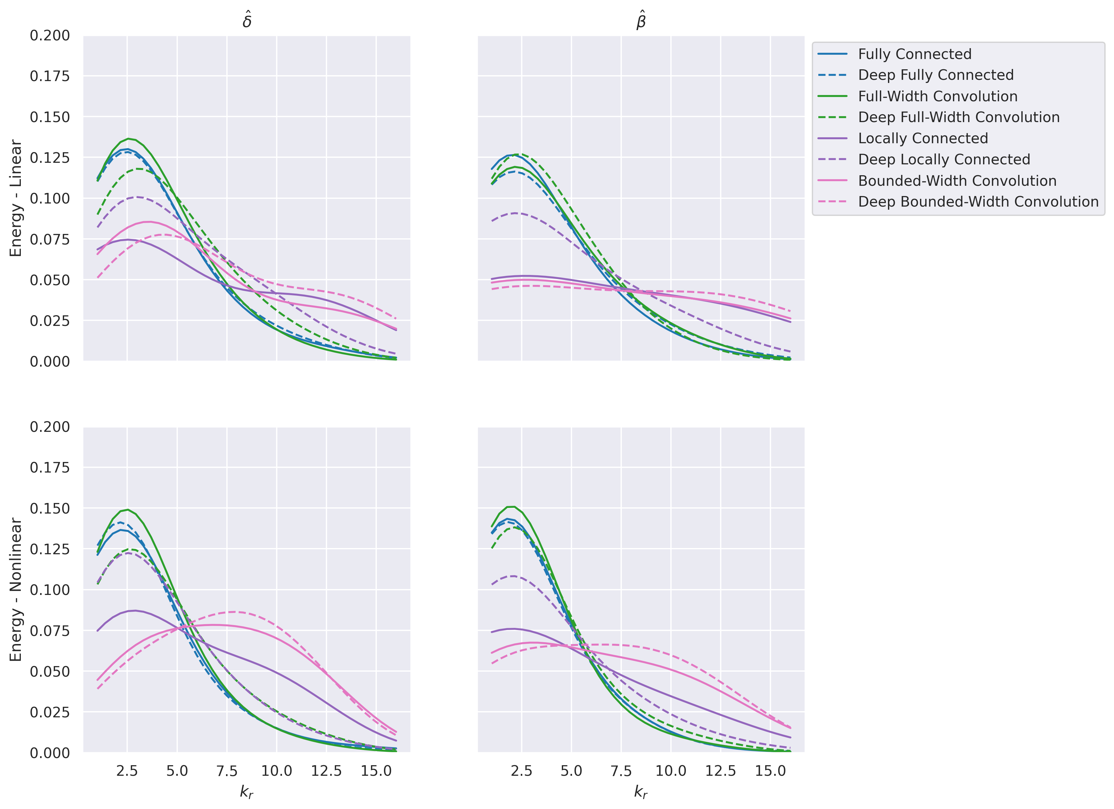
In order to do so we plotted, in Figure 2, for and , the distribution of energy associated to the different frequencies in the spectrum of the perturbation averaging over all 2D directions (radial integral). The Figure shows the radial integral of the adversarial perturbations () for PGD-Linf attack [32] and that of the input-output weight () in the case of CIFAR10 (for the other datasets see Supp Section A.1). We observe that:
The full-width convolutional linear model has a sparser spectrum of compared to the fully connected model, and that when the model has more layers this difference increases (Deep FWC vs Deep FC). This is an experimental confirmation of the theoretical result in [19] for linear models.
The results also show that and share the same spectral structure across all models we analyzed, indicating that the implicit regularizer induced by the model parametrization affects the structure of the adversarial examples. To further verify our results we quantified the different sparsity levels of the two models, measuring the and norm of the Fourier spectrum of for both the shallow and deep full-width and fully connected architectures as reported in Fig 3.
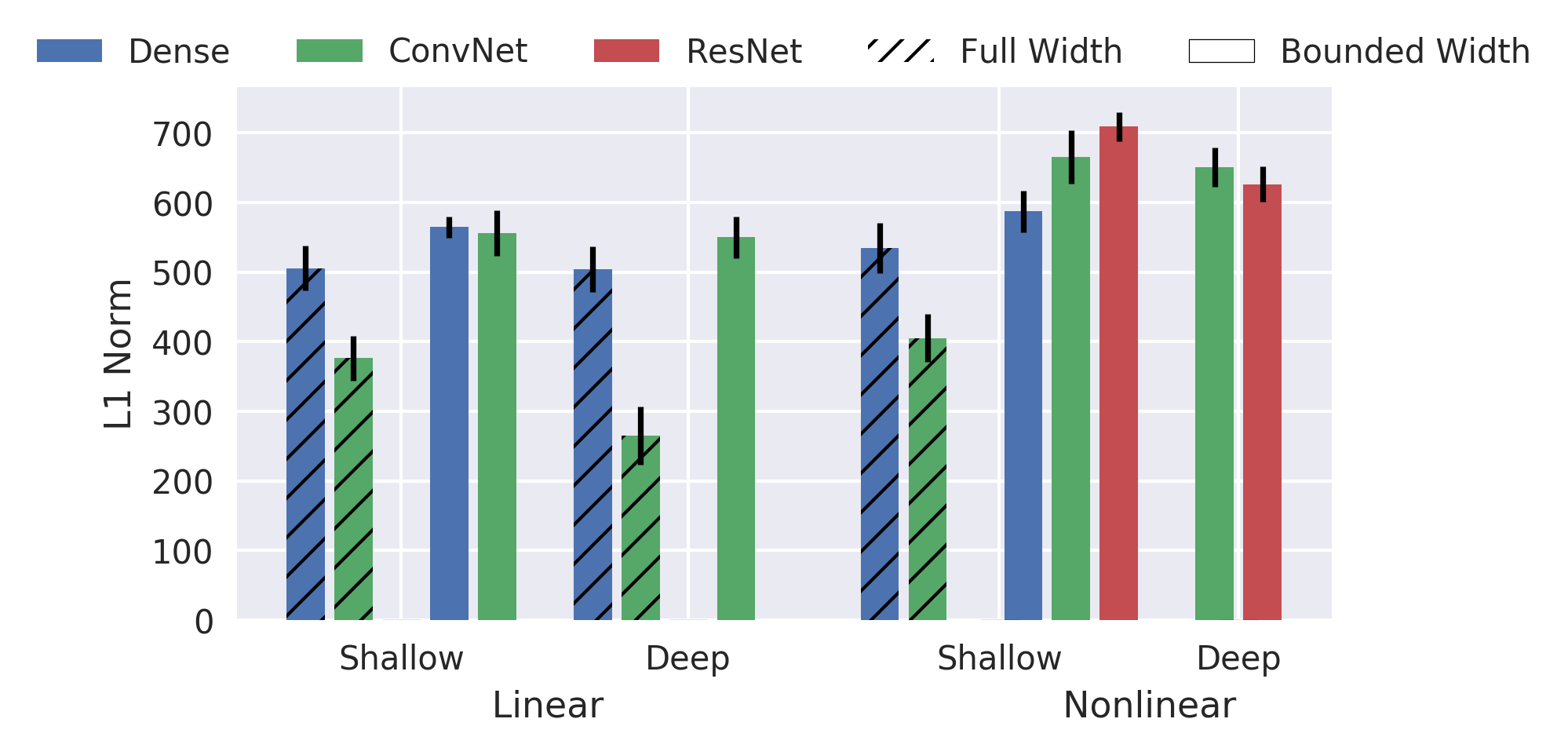
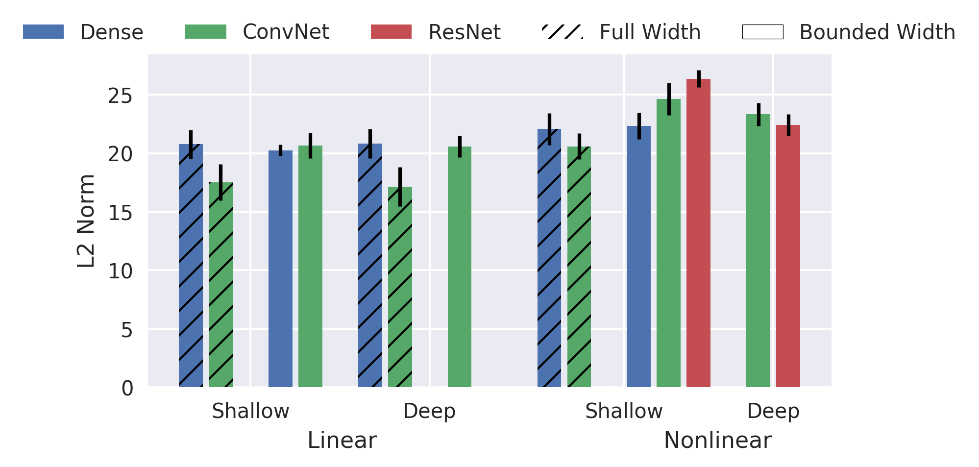
Next, we tested if a similar implicit regularization holds for nonlinear models. As shown in Figure 3 the full-width convolutional model has a sparser spectrum for both and compared to the fully connected model, confirming our hypothesis.
2.2 Bounded-Width Convolutional Models Analysis
One limitation of the analysis done in [19] and in the previous section is that full-width convolutional layers are not often used in common state-of-the-art architectures. Bounded-width convolutional models are instead usually employed, which have smaller kernel sizes than the width of the input. A natural question is therefore: what is the effect of the bounded-width convolutional model on and ?
To answer the question, we trained bounded-width convolutional models and generated both and with the same procedure as the previous section. In Figure 2, we can see that:
The bounded-width convolutional models (both linear and nonlinear) contain high frequency components in and their presence grows with depth in the Deep Bounded-Width model (DBWC). Moreover, we observe that the corresponding to the bounded-width convolutional model is as sparse or less sparse (more dense) compared to the full-width counterpart as reported in Figure 3.
Given that the theory in [19] only specifies a bias towards -sparsity in the frequency domain (i.e. both in the low and high frequencies), why do we observe a bias in the higher frequencies for the bounded-width convolutional model but not the full-width convolutional model? Our experiments suggest that high frequency concentration is due to the fact that convolutional kernels are localized. We propose a theoretical explanation via the Fourier Uncertainty Principle – i.e. a space-limited kernel cannot be band-limited in frequency domain – as the origin of the frequency bias. This reasoning can be made rigorous for a bounded-width linear convolutional model by a simple and straightforward extension of the results of Gunasekar et al, 2018 along with the invocation of energy concentration Uncertainty Principle, resulting in the following theorem:
Theorem 1.
Let be the end to end linear predictor, where is the weights for layer and indicates convolution. Then decreasing the kernel size of each convolutional filter results in an increased concentration of energy in high frequencies for .
A rigorous mathematical treatment can be found in the C. The key intuition is that, due to the Fourier Uncertainty Principle, decreasing the support of the convolutional filter at layer causes an increase of its high frequency energy content.
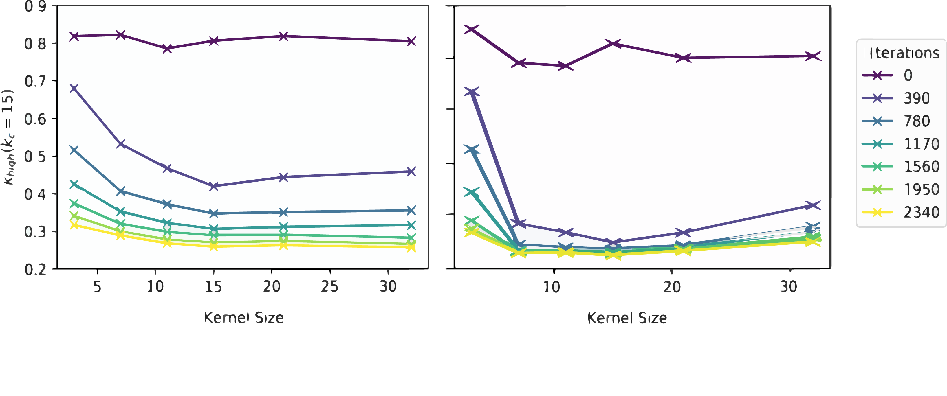
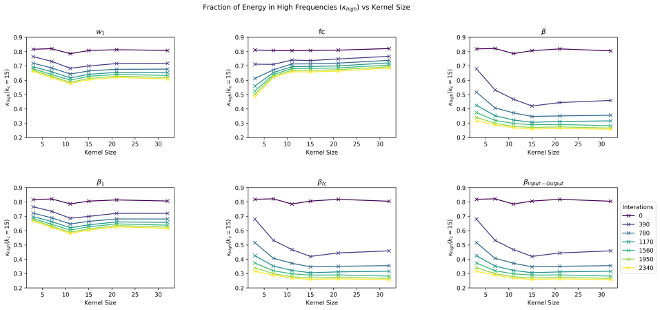
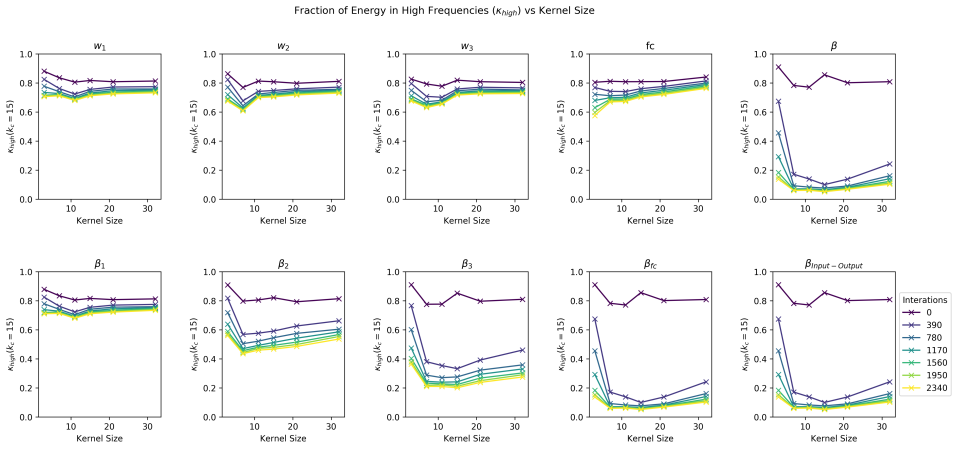
We directly tested our theory on the same models proposed by Gunasekar 2018 but with varying kernel sizes (, , , , , and ), with 1 or 3 hidden layers, and train them on Grayscale CIFAR10. This choice was made to keep the number of hidden channels equal to the number of input channels. Then we computed the frequency spectrum of and the cumulative weights up to layer , . Next we computed , defined as the fraction of energy outside of an interval , where is an specific frequency, divided by the total energy for each kernel. In Figure 4, we observe that the fraction of energy is a function of the kernel size, where for smaller , is higher. Furthermore, as the model goes deeper, the difference is further exacerbated. We observe the same phenomenon both for deeper models and during training (Left). The complete plot with all intermediate layers can be found in the Supplementary Material.
2.3 Role of Translation Invariance in the frequency spectrum of and
Next, to further understand the origin of the high frequency bias, we investigated if the high frequency bias also present in a model with local kernels but not translation invariance (i.e. no shared weights). In other words we tested if convolutionality was essential in determining the high frequency bias. We trained a locally connected model (no convolutional weight sharing) with same kernel size on CIFAR10. In Figure 2 we observe that the locally connected models do not have as much energy in the higher frequencies, particularly for the deep models. The results show that local connectivity alone is not sufficient to bias the model towards learning high frequency features; translation invariance is also required. Thus, local convolutions are necessary to get a bias towards high frequency in the learned features and adversarial perturbations.


Clearly local convolutions are not the only factor. Indeed, as Maiya et al [12] has shown, data-statistics is also an important element in determining the frequency content of adversarial perturbations. Thus we analyzed the compounding effect of model parametrization in the context of different datasets. Towards this goal we computed the cumulative 1D radial integral of and for MNIST, FashionMNIST, SVHN, CIFAR10 and CIFAR100. Then, we estimated the half power frequency () of each model (averaged across different depths and nonlinearities), i.e. the frequency at which we acumulate the total energy. In Figure 5, we observe that the is larger for the Bounded-Width Convolutional Model compared to the Full-Width Convolution, Fully-Connected and Locally Connected models for the all considered datasets (See Sup. Figures 2, 3, 4, 5 for Radial Integral energy of each dataset). These results show that if high frequency useful features are present, the bounded-width convolutions will have more high frequency energy both in and compared to other model parametrizations. Furthermore, even in datasets with more low-frequency information content such as MNIST or FashionMNIST, there is still a smaller but significant bias towards higher frequencies in Bounded-Width Convolutional models.
2.4 Further testing different implicit bias via the Injection of Hidden Shortcut Features
Given that the theory in Gunasekar et al., 2018 doesn’t extend to the implicit regularization for nonlinear convolutional models, we decided to directly test if the implicit bias of nonlinear model parametrizations is similar to that of their linear counterparts.
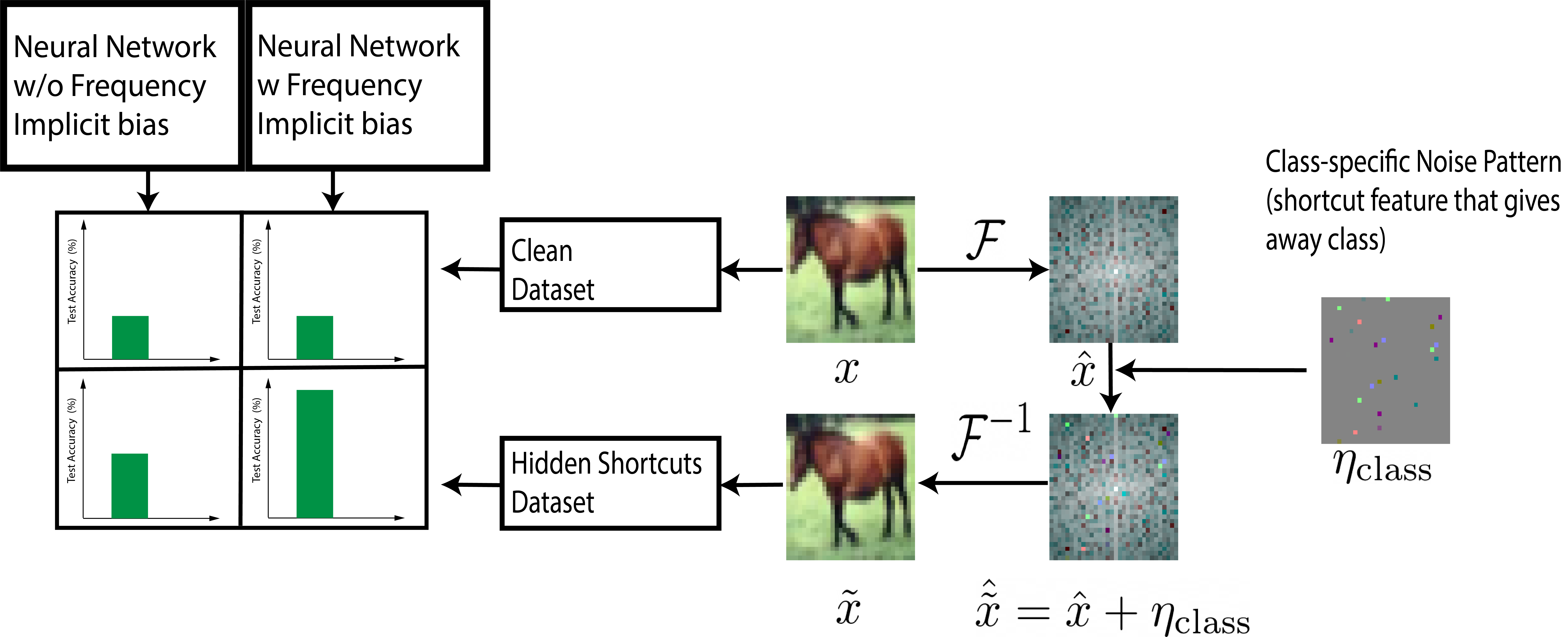
To test our hypothesis, we took inspiration from the field of steganography which focuses on hiding shortcut features in images that are visually undetectable by humans [33]. We introduced a class-correlated sparse shortcut features in Fourier space of every CIFAR-10 train and test set image (See Figure 6). Our hypothesis is that these class-dependent shortcut features will be mostly useful for model parametrizations that have an implicit regularizer that is sparse in the frequency domain. Therefore the model with the right implicit bias should achieve higher test accuracy (for generation of the shortcut features see the Methods section, 3 ). Furthermore, these experiments helped us to further analyze the relationship between the implicit bias due to model parametrization and specific dataset statistics because these new features will now be part of the dataset. Indeed if the model parametrization is not important all models will take advantage of those features and the dataset statistic is the main driver of feature selection.
Baseline Fully Connected Linear 40.8 .070 53.26 .075 45.27 1.14 Fully Connected Nonlinear 48.5 .084 59.6 .223 54.93 .497 Full Width Convolutional Linear 41.8 .124 70.3 .805 79.6 1.35 Full Width Convolutional Nonlinear 52.4 2.89 79.5 .912 87.2 1.26 Bounded Width Convolutional Linear 41.8 .046 97.28 .604 92.33 .679 Bounded Width Convolutional Nonlinear 56.7 .489 98.8 .850 97.8 .475
Models Low Frequency Medium Frequency High Frequency Full-Width Convolution (L=1) 100.0 41.03 41.38 Full-Width Convolution (L=3) 100.0 39.80 40.97 Bounded-Width Convolution (L=1) 100.0 49.99 53.60 Bounded-Width Convolution (L=3) 100.0 94.17 98.47 Fully Connected (L=1) 99.78 41.45 41.38 Fully Connected (L=3) 100.0 46.37 41.21 Locally Connected (L=1) 100.0 44.39 46.23 Locally Connected (L=3) 100.0 47.36 54.73
Table 1 shows the test accuracy of each linear and nonlinear model with the new dataset and different levels of sparsity in the frequency domain. We can observe that both the full-width and bounded-width models have higher performance than baseline with the new dataset. However, the fully connected model, having a different bias, cannot take full advantage of the class-dependent shortcut features introduced into the dataset. This experiment reveals that the implicit regularizer for sparsity in the frequency domain is present in both linear and nonlinear convolutional models.
In addition to these results, we further tested the high frequency bias of the bounded-width parametrization. By performing a new variant of the hidden features experiment, we now localize the information in the low, medium, or high frequencies by introducing the class-dependent signals characterized by frequency in specific bands of the spectrum of the training and testing set of CIFAR10 (See Section 3 for methodological details).
Table 2 shows the performance of the linear models with the new frequency-based class-dependent features. We observe that all models are able to use the low-frequency shortcut features in order to perform the task. Furthermore, when the cheat signal is introduced in the medium and high frequencies the full-width convolutional, fully connected, and locally connected models have a much more difficult time in selecting the signal. On the contrary the Bounded-Width Convolutional Model is able to perform the best in medium and high frequencies compared to the other models and the difference is maintained in deeper models. This experiment not only confirms the presence of an implicit bias due to parametrization in nonlinear ReLU models, but also shows that when useful frequency-based information is present, models with localized convolutions are able to capture those features with more ease compared to other model parametrizations. We compare our results to Wang et al 2020, where they showed that the smoothness of the convolutional models final kernel is the main driver of low frequency bias. Here we show that bounding the kernel has a stronger regularization on the frequency component of the features learned. Furthermore, Tsuzuku et al, 2019 showed that convolution-based models have a preference towards features in the Fourier basis. Here we expand on their results, asking what is the difference between bounded vs full-width convolutions and showing that not all convolution-based models are able to pick up every feature in the Fourier domain.
2.5 Non-convolutional state-of-the-art models do not exhibit a high frequency bias
Since local convolutions cause a bias towards high frequency features and adversarial perturbations, it is natural to ask: are high-performance deep models without convolutions less biased towards high-frequency features? One possible architecture is the Vision Transformer (ViT), which has performed on par with convolution-based architectures in many tasks including object recognition [34]. Furthermore, recent work has shown that ViTs can be more robust to high frequency adversarial perturbations than ResNets [35].
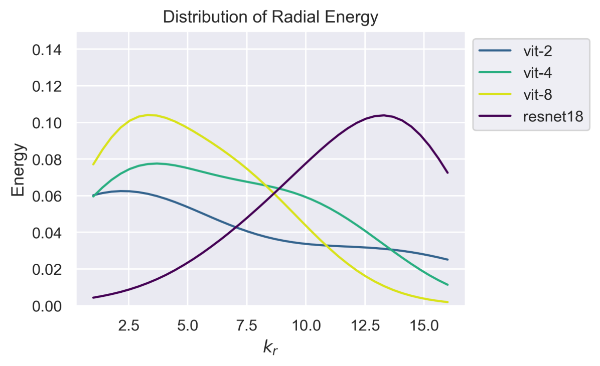

We hypothesize that the lack of convolutional operations in ViTs is responsible for the greater robustness to high frequency attacks. In order to test our hypothesis, we trained a ViT with different patch sizes on CIFAR-10 (See Supp. Sec. B.3 for training details). All of these models achieved about 80 test accuracy. These are lower accuracies than state-of-the-art since those models are usually pretrained on ImageNet, a step we omitted being in the present work only interested in studying the effect of the model architecture. Then, we attacked the models with a PGD-Linf attack, the same used earlier in the paper. In Figure 7(a), we observe the average frequency spectrum of ViTs with different word/patch sizes (, , ), as compared to a ResNet18 with similar test accuracy (we stopped the training when the model had near 80% test accuracy). We observe that all of the ViTs have more energy in the lower frequencies than the ResNet18. This strongly suggests that the robustness to high frequency attacks shown in [35] might be due to the lack of convolution layers. Furthermore, we observe that different patch/word sizes also have an impact on the spectrum, with smaller word sizes producing higher frequency spectra. This is consistent with our theoretical and empirical results comparing full-width and bounded-width convolutional models.
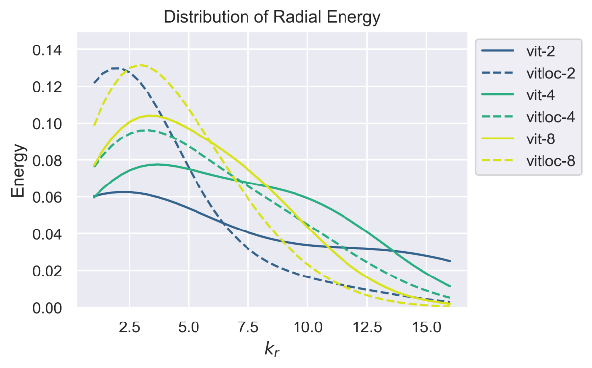
However, as others have suggested, some layers of the ViT can still be interpreted as convolutional layers, so the model is not entirely convolution-free [36]. In particular, the first embedding layer is shared across all image patches, and therefore is a convolutional layer with stride equal to the patch/kernel size. Can we remove this layer and shift the energy spectrum to even lower frequencies? To test for this hypothesis we defined a new ViT architecture in which we removed the weight sharing in the first layer patch embedding by using a locally connected layer with the same kernel size and stride as the convolutional version, so that each patch has independent weights. We call this architecture the Vision Local Transformer (ViTLoc). Then, we trained this architecture on CIFAR-10 (see Performance in Sup. Table 6) and computed the associated adversarial perturbations. In Figure 7(b), we observe that every ViTLoc model has a lower frequency spectrum than its ViT counterpart. This is more evidence that avoiding the convolutional parametrization, even in very complex state-of-the-art models, can reduce the high frequency bias, and therefore, high frequency adversarial perturbations.
2.6 Expanding to State-of-the-art Machine learning models
Here we want to further test the high frequency bias of bounded width convolutional models in models trained on one of the most complex dataset of image recognition: Imagenet [37].
We selected different models from the timm package [38], that are representative of complex models with different model parametrizations. All the models were selected from 4 groups: Convolution-Based Models, Vision Transformers, Hybrid ViT and Convolutional Models, and MLPs models (see Supp Section B.1 for specifics pretrained timm models). All selected models have similar data augmentation procedures since data augmentation can affect the frequency sensitivity of a model [13, 14, 10].
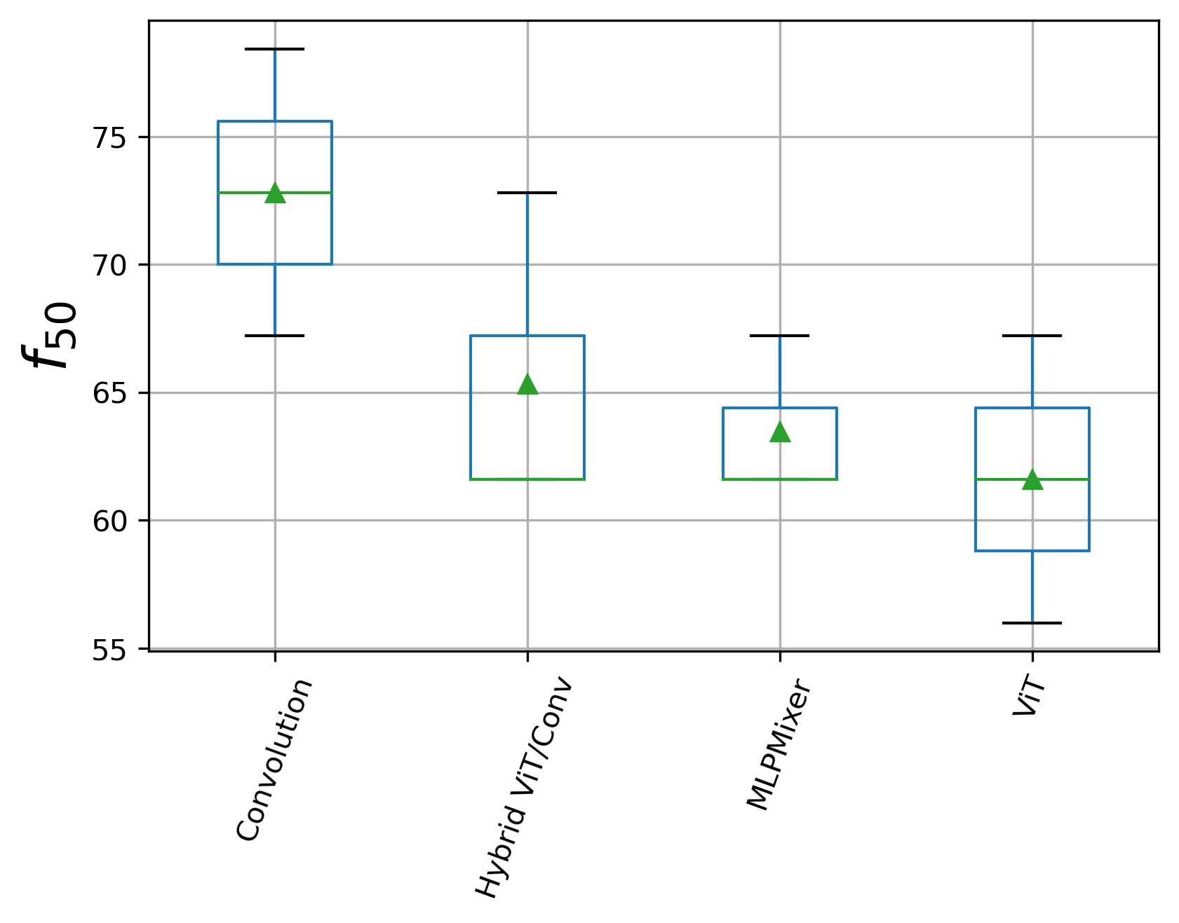
Figure 8 shows the radial integral of the energy of the adversarial perturbations of the ImageNet validation set: we observe that the convolutional-based models (Blue) have less energy in the low frequencies and more in the high frequencies compared to all other models. As for the CIFAR10 dataset, the ViT models (Purple) have lower frequency adversarial. More interestingly, models with larger first layer kernels (ViT (32)) have more energy in the low frequencies compared to models with smaller kernel sizes (ViT(16), ViT(8)). This confirms the results in section 2.5 with models trained on CIFAR10. Interestingly, the work in [39] showed that self-attention layers can produce models with lower frequency preference and that a combination of the Vision Transformers with Convolutions generates a compromise frequency preference. Here we confirm those findings showing that hybrid models already have a in between ViTs and Convolution models and also find that also MLP-Based models have similar energy distribution compared to hybrid models. This indicates that self-attention is not the only mechanism to achieve a low frequency bias, and that the linear layer parametrization seem to be able to achieve similar effects. All together these results show that, regardless of the dataset, convolution-based models have a preferences towards higher frequency features compared to the non-convolutional counterparts.
Conclusions
We provide both empirical as well as theoretical evidence that one of the causes of the high-frequency adversarial examples is the convolutional architecture of modern high-performance networks and, in particular, the locality/boundness of the convolutional kernels. To this end, we first confirmed the theoretical results regarding the network implicit bias in deep linear full-width convolutional models [19], extend them to nonlinear models (section 2.1) and correlate the end-to-end weights of the model with the adversarial perturbation.
We then considered deep linear bounded-width convolutions and derived new theoretical results showing a bias towards high-frequency features compared to other model parametrizations in section 2.2.
In section 2.3 we showed that convolutional weights sharing is a key factor in producing the high frequency bias in networks.
Moreover, by a novel steganography experiment, we could clearly confirm that this bias extends to nonlinear models, and that it strongly influences what features can be easily learned by the models (section 2.4). We think is a new and exciting directions to probe the ability of the model to generalize along any basis not just Fourier. In addition, our work has shown that adversarial perturbations can be an important technique to analyze the features learned by a neural networks at the end or during training.
Furthermore, by using different datasets, we were able to show that convolution-based models have more energy in the high frequencies if high frequency useful information is present. This results deviate from the general understanding of adversarial perturbations and generalization, where high frequency adversarial attacks are only determined by the dataset statistics. Instead, we show that even in datasets with higher frequency information such as CIFAR10, CIFAR100 and SVHN, models with non-convolutional architectures (e.g. fully connected, locally connected, and Vision Transformers) do not present high frequency adversarial attacks (section 2.5). In addition we demonstrated that ViTs with smaller kernel sizes have more energy in the high frequencies for both CIFAR10 and ImageNet trained models, suggesting that these results are robust regardless of dataset statistics. Moreover removing the convolutional layer in ViTs (Local Vision Transformer Architecture), allow us to reduced the energy concentration of Transformer models even further. This shows that one could potentially analyze the implicit bias of different architectural motifs in simple models and extract those principles into more complex scenarios.
However, recent work has shown that self attention does induce a low frequency bias in ViTs [39]. They showed that self-attention layers have a low pass filtering effect on the features received from the previous layer and therefore this is why ViTs are more focused on low-frequency features [39]. Here we show that other non-convolutional architectures such as MLPMixer, ResMLP and gMixer have lower frequency adversarial attacks similar to ViTs even without self-attention layers. This shows that self-attention is not the only mechanism to achieve low-frequency biased models, and that the linear layer parametrization also has a significant effect in this behavior. We think this is important because ViTs, MLPs or Convolution-based models such as ResNets, have multiple components such as Norm Layers, Skip Connections, Attention, Layer Mixing, etc, that may overpower the linear parametrization in defining the implicit bias of the model. However, we found that the linear layer parametrization seem to be crucial to the nature of the features learned and therefore for the adversarial perturbations.
Finally, much work about generalization and adversarial attacks has been centered around bias in datasets [11, 9], however, here we show that attention needs to be paid to the bias caused by architectural choices as well. This work is just the start of establishing the relationship between implicit bias due to model parametrization and the robustness of neural networks to different kinds of input perturbations. We believe this understanding can help drive models towards the most useful set of features and reduce the adversarial susceptibility of modern neural networks.
Acknowledgments
This research has been funded by the NSF NeuroNex program through grant DBI-1707400. This research was also supported by Intelligence Advanced Research Projects Activity (IARPA) via Department of Interior/Interior Business Center (DoI/IBC) contract number D16PC00003. The U.S. Government is authorized to reproduce and distribute reprints for Governmental purposes notwithstanding any copyright annotation thereon. Disclaimer: The views and conclusions contained herein are those of the authors and should not be interpreted as necessarily representing the official policies or endorsements, either expressed or implied, of IARPA, DoI/IBC, or the U.S. Government.
3 Methods
3.1 Neural Network Training.
Each architecture was defined by the number of hidden layers, and nonlinearities (See Supp Table 3). In terms of hyperparameters, we tuned the maximum learning rates for each model by starting from a base learning rate of , and then, if there were visible failures during training (most commonly, the model converging to chance performance), we adjusted the learning rate up/down by a factor of or . Amongst the model architectures we explored, the only hyper-parameter that was tuned was the learning rate. The final values of the learning rates after search are detailed in Table 7. In addition, all the models were trained with linearly decaying learning rate follow factor for each epoch and resetting the learning rate back to max when the model was trained at least epochs. All the models were trained on a single GTX Ti for at least epochs ( to GPU minutes), and we choose the epoch with the highest validation set accuracy for further experiments (see hyperparameters of training and accuracy on Supp Sec. B.3)
3.2 Adversarial Attack Generation.
We used the Foolbox package [40] (MIT license) to generate adversarial perturbations for every example in the test set for a fully trained model (PGD-Linf, PGD-L2, PGD-L1[41], BB-Linf and BB-L2 [42]). Finally, we computed the 2-D Discrete Fourier spectrum of the perturbation . Details of the attacks are available in Supp. Table 12.
3.3 Calculation and Toeplitz Matrix.
For the computation of , we used two different methods. For the linear models, we transformed the weights of every architecture into their matrix form. For example for the convolutional operation, we generated a Toeplitz matrix per convolutional filter and then calculated the dot product of the first matrices to get the (or for all to get the input-output function ). For the nonlinear models, because the nonlinearities does not allow us to use the weights directly, we decided to use a proxy, the saliency map. Saliency Map is the gradient () of the function () with respect to the input image (). In the linear case, these gradients are exactly the weights of the function (up to a constant), which we confirmed using the Toeplitz computation above. For the nonlinear models, because the weights used changed per example, the gradient gave us a good approximation of those weights.
3.4 Generation of Hidden Shortcut Features.
For each class, we sampled a matrix of scalars from a standard Gaussian distribution with mean of 0 and standard deviation of 1 (). Then we multiplied this matrix by a scalar factor , which was selected via hyperparameter search. Next, we generated a masking matrix () of the same size, . For the sparse shorcut feature experiment this matrix was generated from a Bernoulli distribution with an specific average sparsity level . For the frequency-based class dependent features, we selected an upper and lower bound radii as a factor of the max frequency ( and ; and ; and and for the low, medium and high frequencies respectively). These were the ranges used to produce the masking matrix . Next, we computed the hardmard product of with . Then, this class-specific shortcut feature was added into the Fourier spectrum of CIFAR-10 train and test images corresponding to their respective classes. The mathematical definitions are as follows:
References
- Gilmer et al. [2018] Justin Gilmer, Luke Metz, Fartash Faghri, Samuel S Schoenholz, Maithra Raghu, Martin Wattenberg, and Ian Goodfellow. Adversarial spheres. arXiv preprint arXiv:1801.02774, 2018.
- Mahloujifar et al. [2019] Saeed Mahloujifar, Dimitrios I Diochnos, and Mohammad Mahmoody. The curse of concentration in robust learning: Evasion and poisoning attacks from concentration of measure. In Proceedings of the AAAI Conference on Artificial Intelligence, volume 33, pages 4536–4543, 2019.
- Tanay and Griffin [2016] Thomas Tanay and Lewis Griffin. A boundary tilting persepective on the phenomenon of adversarial examples. arXiv preprint arXiv:1608.07690, 2016.
- Ford et al. [2019] Nic Ford, Justin Gilmer, Nicolas Carlini, and Dogus Cubuk. Adversarial examples are a natural consequence of test error in noise. arXiv preprint arXiv:1901.10513, 2019.
- Fawzi et al. [2018] Alhussein Fawzi, Hamza Fawzi, and Omar Fawzi. Adversarial vulnerability for any classifier. In Advances in Neural Information Processing Systems, pages 1178–1187, 2018.
- Bubeck et al. [2018] Sébastien Bubeck, Eric Price, and Ilya Razenshteyn. Adversarial examples from computational constraints. arXiv preprint arXiv:1805.10204, 2018.
- Goodfellow et al. [2014] Ian J Goodfellow, Jonathon Shlens, and Christian Szegedy. Explaining and harnessing adversarial examples. arXiv preprint arXiv:1412.6572, 2014.
- Schmidt et al. [2018] Ludwig Schmidt, Shibani Santurkar, Dimitris Tsipras, Kunal Talwar, and Aleksander Madry. Adversarially robust generalization requires more data. In Advances in Neural Information Processing Systems, pages 5014–5026, 2018.
- Ilyas et al. [2019] Andrew Ilyas, Shibani Santurkar, Dimitris Tsipras, Logan Engstrom, Brandon Tran, and Aleksander Madry. Adversarial examples are not bugs, they are features. In Advances in Neural Information Processing Systems, pages 125–136, 2019.
- Yin et al. [2019] Dong Yin, Raphael Gontijo Lopes, Jonathon Shlens, Ekin D. Cubuk, and Justin Gilmer. A Fourier Perspective on Model Robustness in Computer Vision. Curran Associates Inc., Red Hook, NY, USA, 2019.
- Wang et al. [2020] Haohan Wang, Xindi Wu, Zeyi Huang, and Eric P Xing. High-frequency component helps explain the generalization of convolutional neural networks. In Proceedings of the IEEE/CVF Conference on Computer Vision and Pattern Recognition, pages 8684–8694, 2020.
- Maiya et al. [2021] Shishira R Maiya, Max Ehrlich, Vatsal Agarwal, Ser-Nam Lim, Tom Goldstein, and Abhinav Shrivastava. A frequency perspective of adversarial robustness. arXiv preprint arXiv:2111.00861, 2021.
- Li et al. [2022] Zhe Li, Josue Ortega Caro, Evgenia Rusak, Wieland Brendel, Matthias Bethge, Fabio Anselmi, Ankit B Patel, Andreas S Tolias, and Xaq Pitkow. Robust deep learning object recognition models rely on low frequency information in natural images. bioRxiv, 2022.
- Hermann et al. [2020] Katherine Hermann, Ting Chen, and Simon Kornblith. The origins and prevalence of texture bias in convolutional neural networks. Advances in Neural Information Processing Systems, 33:19000–19015, 2020.
- Geirhos et al. [2018] Robert Geirhos, Patricia Rubisch, Claudio Michaelis, Matthias Bethge, Felix A Wichmann, and Wieland Brendel. Imagenet trained cnns are biased towards texture; increasing shape bias improves accuracy and robustness. arXiv preprint arXiv:1811.12231, 2018.
- Tsuzuku and Sato [2019] Yusuke Tsuzuku and Issei Sato. On the structural sensitivity of deep convolutional networks to the directions of fourier basis functions. In Proceedings of the IEEE/CVF Conference on Computer Vision and Pattern Recognition, pages 51–60, 2019.
- Ortiz-Jimenez et al. [2020a] Guillermo Ortiz-Jimenez, Apostolos Modas, Seyed-Mohsen Moosavi-Dezfooli, and Pascal Frossard. Hold me tight! influence of discriminative features on deep network boundaries. arXiv preprint arXiv:2002.06349, 2020a.
- Ortiz-Jimenez et al. [2020b] Guillermo Ortiz-Jimenez, Apostolos Modas, Seyed-Mohsen Moosavi-Dezfooli, and Pascal Frossard. Neural anisotropy directions. arXiv preprint arXiv:2006.09717, 2020b.
- Gunasekar et al. [2018] Suriya Gunasekar, Jason D Lee, Daniel Soudry, and Nati Srebro. Implicit bias of gradient descent on linear convolutional networks. In Advances in Neural Information Processing Systems, pages 9461–9471, 2018.
- Yun et al. [2020] Chulhee Yun, Shankar Krishnan, and Hossein Mobahi. A unifying view on implicit bias in training linear neural networks. arXiv preprint arXiv:2010.02501, 2020.
- Sahs et al. [2020a] Justin Sahs, Aneel Damaraju, Ryan Pyle, Onur Tavaslioglu, Josue Ortega Caro, Hao Yang Lu, and Ankit Patel. A functional characterization of randomly initialized gradient descent in deep re{lu} networks, 2020a. URL https://openreview.net/forum?id=BJl9PRVKDS.
- Williams et al. [2019] Francis Williams, Matthew Trager, Daniele Panozzo, Claudio Silva, Denis Zorin, and Joan Bruna. Gradient dynamics of shallow univariate relu networks. In Advances in Neural Information Processing Systems, pages 8376–8385, 2019.
- Woodworth et al. [2020] Blake Woodworth, Suriya Gunasekar, Jason D Lee, Edward Moroshko, Pedro Savarese, Itay Golan, Daniel Soudry, and Nathan Srebro. Kernel and rich regimes in overparametrized models. arXiv preprint arXiv:2002.09277, 2020.
- Sahs et al. [2020b] Justin Sahs, Ryan Pyle, Aneel Damaraju, Josue Ortega Caro, Onur Tavaslioglu, Andy Lu, and Ankit Patel. Shallow univariate relu networks as splines: Initialization, loss surface, hessian, & gradient flow dynamics. arXiv preprint arXiv:2008.01772, 2020b.
- Li et al. [2019] Zhiyuan Li, Ruosong Wang, Dingli Yu, Simon S Du, Wei Hu, Ruslan Salakhutdinov, and Sanjeev Arora. Enhanced convolutional neural tangent kernels. arXiv preprint arXiv:1911.00809, 2019.
- Arora et al. [2019] Sanjeev Arora, Simon S Du, Wei Hu, Zhiyuan Li, Russ R Salakhutdinov, and Ruosong Wang. On exact computation with an infinitely wide neural net. In Advances in Neural Information Processing Systems, pages 8139–8148, 2019.
- Krizhevsky et al. [2009] Alex Krizhevsky, Geoffrey Hinton, et al. Learning multiple layers of features from tiny images. 2009.
- LeCun and Cortes [2010] Yann LeCun and Corinna Cortes. MNIST handwritten digit database. 2010. URL http://yann.lecun.com/exdb/mnist/.
- Xiao et al. [2017] Han Xiao, Kashif Rasul, and Roland Vollgraf. Fashion-mnist: a novel image dataset for benchmarking machine learning algorithms, 2017. URL http://arxiv.org/abs/1708.07747.
- Netzer et al. [2011] Yuval Netzer, Tao Wang, Adam Coates, Alessandro Bissacco, Bo Wu, and Andrew Y. Ng. Reading digits in natural images with unsupervised feature learning. In NIPS Workshop on Deep Learning and Unsupervised Feature Learning 2011, 2011.
- Paszke et al. [2019] Adam Paszke, Sam Gross, Francisco Massa, Adam Lerer, James Bradbury, Gregory Chanan, Trevor Killeen, Zeming Lin, Natalia Gimelshein, Luca Antiga, et al. Pytorch: An imperative style, high-performance deep learning library. Advances in neural information processing systems, 32:8026–8037, 2019.
- Madry et al. [2017] Aleksander Madry, Aleksandar Makelov, Ludwig Schmidt, Dimitris Tsipras, and Adrian Vladu. Towards deep learning models resistant to adversarial attacks. arXiv preprint arXiv:1706.06083, 2017.
- Cheddad et al. [2010] Abbas Cheddad, Joan Condell, Kevin Curran, and Paul Mc Kevitt. Digital image steganography: Survey and analysis of current methods. Signal processing, 90(3):727–752, 2010.
- Dosovitskiy et al. [2020] Alexey Dosovitskiy, Lucas Beyer, Alexander Kolesnikov, Dirk Weissenborn, Xiaohua Zhai, Thomas Unterthiner, Mostafa Dehghani, Matthias Minderer, Georg Heigold, Sylvain Gelly, et al. An image is worth 16x16 words: Transformers for image recognition at scale. arXiv preprint arXiv:2010.11929, 2020.
- Shao et al. [2021] Rulin Shao, Zhouxing Shi, Jinfeng Yi, Pin-Yu Chen, and Cho-Jui Hsieh. On the adversarial robustness of visual transformers. arXiv preprint arXiv:2103.15670, 2021.
- Chen et al. [2021] Zhengsu Chen, Lingxi Xie, Jianwei Niu, Xuefeng Liu, Longhui Wei, and Qi Tian. Visformer: The vision-friendly transformer. arXiv preprint arXiv:2104.12533, 2021.
- Deng et al. [2009] Jia Deng, Wei Dong, Richard Socher, Li-Jia Li, Kai Li, and Li Fei-Fei. Imagenet: A large-scale hierarchical image database. In 2009 IEEE Conference on Computer Vision and Pattern Recognition, pages 248–255, 2009.
- Wightman [2019] Ross Wightman. Pytorch image models. https://github.com/rwightman/pytorch-image-models, 2019.
- Park and Kim [2022] Namuk Park and Songkuk Kim. How do vision transformers work? arXiv preprint arXiv:2202.06709, 2022.
- Rauber et al. [2017] Jonas Rauber, Wieland Brendel, and Matthias Bethge. Foolbox: A python toolbox to benchmark the robustness of machine learning models. arXiv preprint arXiv:1707.04131, 2017.
- Kurakin et al. [2016] Alexey Kurakin, Ian Goodfellow, and Samy Bengio. Adversarial examples in the physical world. arXiv preprint arXiv:1607.02533, 2016.
- Brendel et al. [2019] Wieland Brendel, Jonas Rauber, Matthias Kümmerer, Ivan Ustyuzhaninov, and Matthias Bethge. Accurate, reliable and fast robustness evaluation. In Advances in Neural Information Processing Systems, pages 12861–12871, 2019.
- Ghobber and Jaming [2011] Saifallah Ghobber and Philippe Jaming. On uncertainty principles in the finite dimensional setting. Linear algebra and its applications, 435(4):751–768, 2011.
Appendix A Supplementary Material
A.1 Radial energy distribution for different Datasets
![[Uncaptioned image]](/html/2006.11440/assets/plot_1D_cifar10.png)
![[Uncaptioned image]](/html/2006.11440/assets/plot_1D_cifar100.png)
![[Uncaptioned image]](/html/2006.11440/assets/plot_1D_FashionMNIST.png)
![[Uncaptioned image]](/html/2006.11440/assets/plot_1D_MNIST.png)
![[Uncaptioned image]](/html/2006.11440/assets/plot_1D_SVHN.png)
![[Uncaptioned image]](/html/2006.11440/assets/plot_1D_imagenet.png)
![[Uncaptioned image]](/html/2006.11440/assets/spectrum_different_attacks_final.png)
![[Uncaptioned image]](/html/2006.11440/assets/spectrum_different_attacks_relu_final.png)
A.2 Tables
Model Fully Connected 20.77 1.23 505.95 32.22 546.89 43.37 2232.46 166.27 Full Width Convolution 17.52 1.56 376.31 32.66 544.83 42.40 1598.37 181.44 Bounded Width Convolution 20.65 1.09 556.32 32.64 500.67 47.46 2623.04 331.42 Deep Fully Connected 20.83 1.25 503.92 32.62 554.16 38.95 2168.06 134.07 Deep Full Width Convolution 17.13 1.68 265.40 41.72 522.99 39.72 1417.68 213.91 Deep Bounded Width Convolution 20.57 0.94 550.30 29.71 498.52 47.15 2392.09 278.55
| Model | ||
|---|---|---|
| Fully Connected | 22.06 1.35 | 534.34 35.93 |
| Locally Connected | 22.32 1.13 | 587.61 29.89 |
| Full Width Convolution | 20.57 1.11 | 405.49 34.16 |
| Bounded Width Convolution | 24.63 1.36 | 665.22 38.55 |
| Shallow ResNet | 26.36 0.74 | 709.06 20.76 |
| VGG19 | 23.32 0.99 | 650.73 27.87 |
| ResNet18 | 22.42 0.91 | 626.60 25.40 |
Appendix B Experimental Details
B.1 Model Architecture
Model Architecture Hidden Layers Nonlinearity Channels Fully Connected 1,3 None, ReLU 3072 Bounded Width Convolution 1,3 None, ReLU 32 Full Width Convolution 1,3 None, ReLU 32 Locally Connected 1,3 None, ReLU 32
| Model | Model Type | Model timm package name |
|---|---|---|
| ResNet50 | Convolutional | resnet50d |
| EfficientNet | Convolutional | tf_efficientnet_b0_ns |
| RepVGG | Convolutional | repvgg_b3 |
| ConvViT | Hybrid | convit_base |
| ViT-ResNet50 | Hybrid | vit_large_r50_s32_224 |
| Coat | Hybrid | coat_lite_small |
| ResMLP (36) | MLP | resmlp_36_distilled_224 |
| gMixer | MLP | gmixer_24_224 |
| MLPMixer Large | MLP | mixer_b16_224 |
| ViT (8) | ViT | vit_base_patch8_224 |
| ViT (16) | ViT | vit_base_patch16_224 |
| ViT (32) | ViT | vit_base_patch32_224 |
All ImageNet models were pull from the timm package . Furthermore, all models were trained with similar data augmentations, and adversarial attack evaluation was done with default preprocessing from .
B.2 Model Performance
Test Accuracy (%) Models FashionMNIST MNIST SVHN cifar10 cifar100 Fully Connected 86.9 92.0 26.5 39.6 15.8 Full-Width Convolution 86.6 91.0 28.7 40.5 17.7 Locally Connected 86.4 92.0 28.5 40.7 18.3 Bounded-Width Convolution 86.4 92.0 28.2 40.2 16.1 Deep Full-Width Convolution 86.5 91.8 26.0 41.7 18.9 Deep Fully Connected 86.7 92.1 23.8 39.2 14.7 Deep Locally Connected 84.1 92.0 29.0 41.8 18.8 Deep Bounded-Width Convolution 86.1 92.0 27.7 39.9 14.9 Fully Connected (ReLU) 88.4 97.2 77.6 43.6 15.4 Full-Width Convolution (ReLU) 84.8 92.8 85.9 47.7 19.2 Locally Connected (ReLU) 87.8 95.7 82.4 53.8 22.5 Bounded-Width Convolution (ReLU) 90.5 98.0 83.2 59.7 29.0 Deep Full-Width Convolution (ReLU) 87.8 97.4 86.3 51.7 22.2 Deep Fully Connected (ReLU) 89.1 97.9 67.3 50.8 10.5 Deep Locally Connected (ReLU) 86.5 96.0 86.9 57.9 18.3 Deep Bounded-Width Convolution (ReLU) 91.7 98.8 86.7 66.0 29.6 ViT-2 79.8 ViT-4 80.1 ViT-8 78.4 ViTLoc-2 75.3 ViTLoc-4 80.2 ViTLoc-8 74.5 ResNet18 91.8
| model | top1 | top5 |
|---|---|---|
| vit_base_patch8_224 | 85.794 | 97.794 |
| vit_base_patch16_224 | 84.528 | 97.294 |
| vit_large_r50_s32_224 | 84.424 | 97.166 |
| coat_lite_small | 82.304 | 95.848 |
| convit_base | 82.286 | 95.938 |
| resmlp_36_distilled_224 | 81.154 | 95.488 |
| vit_base_patch32_224 | 80.722 | 95.566 |
| resnet50d | 80.522 | 95.162 |
| repvgg_b3 | 80.496 | 95.264 |
| tf_efficientnet_b0_ns | 78.658 | 94.378 |
| gmixer_24_224 | 78.036 | 93.670 |
| mixer_b16_224 | 76.612 | 92.228 |
B.3 Training Hyperparameters
Model Architecture Learning Rate Batch Size Learning Rate Drop Bounded Width Convolution .01 128 Yes Fully Connected .01 128 Yes Locally Connected .01 128 Yes Full Width Convolution .002 128 Yes Bounded Width Convolution .002 128 Yes
Model Architecture Learning Rate Batch Size Learning Rate Drop Bounded Width Convolution .01 128 Yes Fully Connected .01 128 Yes Locally Connected .01 128 Yes Full Width Convolution .002 128 Yes Bounded Width Convolution .002 128 Yes
Model Architecture Learning Rate Batch Size Learning Rate Drop Bounded Width Convolution .01 100 Yes Fully Connected .01 100 Yes Locally Connected .01 100 Yes Full Width Convolution .002 100 Yes Bounded Width Convolution .002 100 Yes
Model Architecture Learning Rate Batch Size Learning Rate Drop Bounded Width Convolution .01 100 Yes Fully Connected .01 100 Yes Locally Connected .01 100 Yes Full Width Convolution .002 100 Yes Bounded Width Convolution .002 100 Yes
Model Architecture Learning Rate Batch Size Learning Rate Drop Bounded Width Convolution .01 128 Yes Fully Connected .01 128 Yes Locally Connected .01 128 Yes Full Width Convolution .002 128 Yes Bounded Width Convolution .002 128 Yes
B.4 Adversarial Attack Configurations
Attack Metric Learning Rate Number of Steps Max Norm, Projected Gradient Descent 0.1 1000 8.0/255.0 Projected Gradient Descent 0.1 1000 2.0 Projected Gradient Descent 0.1 200 0.1 Brendel-Bethge Attack 1e-03 1000 - Brendel-Bethge Attack 1e-03 1000 -
Learning Rates. All the models adversarial attacks were generated using the configuration above with the Foolbox package [40].
Appendix C Formal Proofs of High Frequency Bias
See 1
Proof.
Let us first concentrate on a single convolutional filter . Given an arbitrary choice of frequency interval and space interval , we want to prove that reducing the energy fraction in the complementary set implies that we must increase the energy fraction in the complementary set . The result follows from a direct application of the Uncertainty Principle for finite-dimensional vector spaces, as shown e.g. in Ghobber-Jaming [43]. In particular let be the coefficients of the Discrete Fourier Transform (DFT) of a convolutional filter . From equation 1.2 in [43] we have
| (1) |
where is constant when the intervals are fixed. Dividing both sides of the inequality by we have
where is the spatial energy concentration of in the index set and is the frequency energy concentration of in the set .
Thus increasing the energy concentration in the spatial interval will cause a decrease in and by the inequality above an increase in . If we let be an interval of ‘low’ frequencies, then we conclude there will be an increase in the energy concentration in the ‘high’ frequencies .
The reasoning above can be extended from a single convolutional filter to the full end-to-end weights vector, , as follows. Note first that, using the convolution theorem, the Discrete Fourier transform of is the Hadamard product of the Discrete Fourier transforms of the per-layer weights i.e.
Let us consider the energy in a set of ‘low’ frequencies :
Taking the norm and invoking the inequality a total of times we can then write
Suppose now that, all else equal, we decrease the energy concentration in each spatial domain of the per-layer filters . By the reasoning above this will increase the energy concentration in frequency domain in the interval i.e. a decrease in for each layer . By the last inequality this will decrease , resulting in an increase in the energy concentration in the high frequencies () for . ∎
Lemma 2.
Concentrating the kernel energy in spatial domain increases the implicit regularization term in the optimization in [Gunasekar]:
Proof.
Reducing filter size will increase energy in high freqs i.e. . This means that the space-limiting constraints only grow more stringent as we reduce , implying that the result of the optimization problem for the implicit regularizer will only increase in cost i.e. for any candidate linear predictor . (Note that this does not refer to the learned features which actually depends on the training data as well). In summary, all else being equal, reducing the kernel size causes/induces a bias towards more concentration of energy in higher frequencies in . ∎
In summary reducing the kernel size causes/induces a bias towards more concentration of energy in higher frequencies in .