Obliquity of an Earth-like planet from frequency modulation of its direct imaged lightcurve: mock analysis from general circulation model simulation
Abstract
Direct-imaging techniques of exoplanets have made significant progress recently, and will eventually enable to monitor photometric and spectroscopic signals of earth-like habitable planets in the future. The presence of clouds, however, would remain as one of the most uncertain components in deciphering such direct-imaged signals of planets. We attempt to examine how the planetary obliquity produce different cloud patterns by performing a series of GCM (General Circulation Model) simulation runs using a set of parameters relevant for our Earth. Then we use the simulated photometric lightcurves to compute their frequency modulation due to the planetary spin-orbit coupling over an entire orbital period, and attempt to see to what extent one can estimate the obliquity of an Earth-twin. We find that it is possible to estimate the obliquity of an Earth-twin within the uncertainty of several degrees with a dedicated 4 m space telescope at 10 pc away from the system if the stellar flux is completely blocked. While our conclusion is based on several idealized assumptions, a frequency modulation of a directly-imaged earth-like planet offers a unique methodology to determine its obliquity.
1 Introduction
Direct-imaging of Earth-like planets is a quite challenging but indispensable technique to revolutionize our understanding of planets in the near future. The amplitude modulation of a photometric lightcurve from a color-changing dot is sensitive to its surface pattern, and thus would reveal the presence of lands, oceans, clouds and even vegetation on the surface of the planets (e.g., Sagan et al., 1993; Ford et al., 2001; Cowan et al., 2009; Oakley & Cash, 2009; Fujii et al., 2010, 2011; Suto, 2019; Rushby et al., 2019). Indeed, continuous monitoring of oblique planets over their orbital periods may even enable one to reconstruct their two-dimensional surface map (Kawahara & Fujii, 2010, 2011; Fujii & Kawahara, 2012; Farr et al., 2018). The feasibility of the mapping has recently been tested using continuous Earth observations by Deep Space Climate Observatory orbiting at an altitude of 150 km (Jiang et al., 2018; Fan et al., 2019; Aizawa et al., 2020).
In addition, the lightcurve carries complementary information for the planet as well. The auto-correlation analysis of the photometric variation roughly provides us the rotation period of the planet (Pallé et al., 2008). The obliquity can also be inferred from a simultaneous fitting of the spin vector and planet surface (e.g. Kawahara & Fujii, 2010; Schwartz et al., 2016; Farr et al., 2018). Such dynamical parameters of the planet are of interest for a general circulation modeling of Earth-like planets (e.g. Kaspi & Showman, 2015; Deitrick et al., 2018; Komacek et al., 2019).
Strictly speaking, an apparent photometric period observed by a distant observer is not necessarily identical to the true spin rotation period due to the planetary orbital motion. This is related to the reason why a sidereal day of our Earth is approximately hours, which corresponds to the true spin frequency [day-1], instead of the [day-1]. The difference between the observed and true spin rotation frequencies, and , is time-dependent, and sensitive to the geometrical configuration of the system including the planetary obliquity, , the inclination of the planetary orbital plane for the observer, , and the observer’s direction (the orbital phase angle measured from the ascending node, for instance).
Thus the corresponding frequency modulation of the periodicity in the lightcurve may reveal those parameters, through the presence of the large-scale inhomogeneity of the surface. We emphasize that the frequency modulation signal is much less sensitive to the specific distribution pattern of the surface than the amplitude modulation. Kawahara (2016, hereafter K16) proposed a novel idea to measure the planetary obliquity from the frequency modulation, and demonstrated its feasibility successfully using a static cloud-subtracted Earth model.
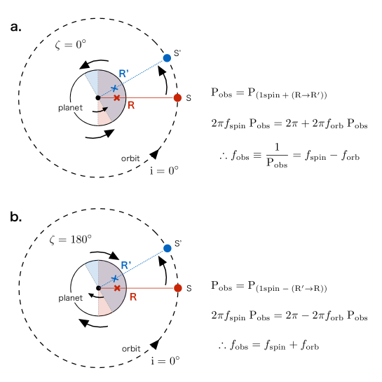
The basic principle of frequency modulation can be understood from Figure 1. For a perfectly prograde planet (), the illuminated and visible part of the planet viewed from a face-on observer () moves along the same direction of the planetary spin (Panel a). The reflective point, at which the reflected flux of the star is maximal on the planetary surface, moves accordingly, and thus it takes slightly more than one spin rotation period for the observer to see the exactly same part of the planet. Therefore the observed photometric variation frequency becomes . Applying the same argument, one can easily understand that for a perfectly retrograde planet () as illustrated in Panel b of Figure 1.
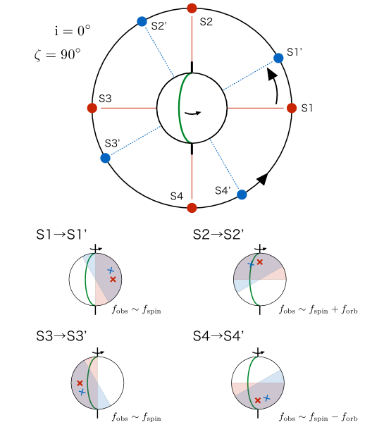
In general, the photometric variation frequency is not constant and varies according to the mutual geometry between the star and the planet, leading to a frequency modulation of the photometric lightcurve of the planet. Figure 2 illustrates an example of the time-dependent frequency modulation for a planet viewed from a distant observer at . In this case, the motion of the reflective point on the planetary surface changes the direction relative to the planetary spin axis in a time-dependent fashion, resulting in the frequency modulation of the observed period.
When the star is located in S1 (and also in S3), the reflective point on the planetary surface moves along the constant longitude, and the planet exhibits a nearly same illuminated and visible part of its surface after one spin rotation period. This implies that . In contrast, when the star is located at S2 (S4), the reflective point after one spin rotation period moves slightly westward (eastward), leading to ().
While the above frequency modulation is basically determined by the geometrical configuration of the system characterized by , , and as mentioned above (see also Figure 3 below), the most important uncertain factor in modeling the lightcurve is the time-dependent cloud pattern. A planet completely covered by the thick homogeneous clouds, for instance, does not exhibit any photometric variation, and thus one cannot probe the surface information at all. In the case of our Earth, approximately 50-60 percent of the surface is covered by clouds on average. Thus, it is not clear to what extent the interpretation from the frequency modulation of the lightcurve is affected or even biased by the properties and time-dependent distribution pattern of clouds.
Since the planetary obliquity is supposed to sensitively change the cloud pattern among others, the feasibility study of the obliquity measurement from the frequency modulation requires a self-consistent modeling of clouds over the entire surface of a planet. This is why we perform the GCM (General Circulation Model)111“General Climate Model” is also referred to as GCM. The two terms are often used interchangeably, but sometimes “General Circulation Model” is more specifically implies a part of modules in “General Climate Model”. In this sense, our model may be referred to as “an atmospheric General Circulation Model”, but we do not distinguish between them in the present paper. simulation and analyze the simulated lightcurves for different planetary obliquities.
The rest of the paper is organized as follows. Section 2 describes the basic model of the frequency modulation in the lightcurve, the GCM simulation of the Earth with different obliquities, and radiation transfer to simulate lightcurves. Section 3 shows the analysis method of the frequency modulation and the result of the frequency modulation signal extracted from simulated lightcurves. Finally section 4 is devoted to the summary and conclusion of the present paper.
2 Computational Methods
2.1 Basic strategy to estimate the planetary obliquity from photometric variation
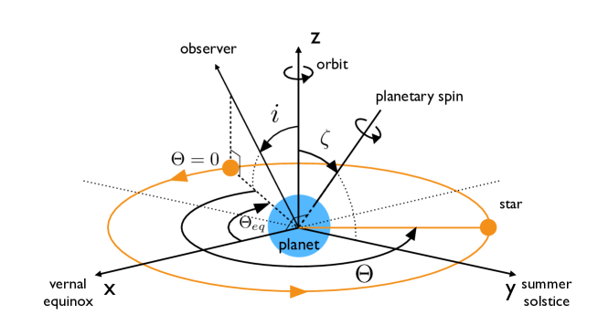
For simplicity, we consider a star-planet system in a circular orbit, which is schematically illustrated in Figure 3. In order to compute the photometric variation of the planet, it is convenient to define a geocentric frame in which the planet is located at the origin. The stellar orbit defines the -plane, and the star orbits around the -axis in a counter-clockwise manner. The unit vector of the planetary spin is on the -plane, and expressed as in terms of the planetary obliquity . Thus the direction of the -axis corresponds to that of the vernal equinox.
The unit vector toward a distant observer is given by , where is the inclination, and is the phase angle measured clockwise from the -axis (i.e., the vernal equinox).
In this frame, the location of the star on the orbit is specified by its phase angle measured from the observer’s projected direction. Since we consider a circular orbit below, (mod ).
K16 computed the frequency modulation based on a maximum-weighted longitude approximation, and derived the following formula for in the case of a circular orbit:
| (1) |
where is the modulation factor 222Equation 2 is the correct version of equation (13) in K16, which contains a couple of typos in signs.,
| (2) |
We apply the maximum-weighted longitude approximation and derive a general formula for non-circular orbits in Appendix A. In the present analysis, however, we focus on a circular orbit, and adopt equation (2) for the frequency modulation template.
Following K16, we use the pseudo-Wigner distribution to estimate the frequency modulation of the photometric variation of a given lightcurve. The pseudo-Wigner distribution is the Fourier transform of the auto-correlation of the data, emphasizing the periodicity near the time of interest, and reducing the cross terms and noises. Further detail will be described in Section 3.
2.2 GCM simulation of the Earth with different obliquities
We would like to emphasize that the main purpose of the present paper is to examine the feasibility of the planetary obliquity measurement through the frequency modulation of the lightcurve. The cloud covering pattern and fraction are important factors that would degrade the measurement. On the other hand, the precise modeling of the climate is not supposed to be essential for the feasibility. Therefore various assumptions and limitations of our current GCM simulation described below need to be clarified and understood, but do not change the main conclusion of the present paper.
We use the GCM code DCPAM5 (the Dennou-Club Planetary Atmospheric Model), which has been developed by GFD-Dennou Club333http://www.gfd-dennou.org/, and http://www.gfd-dennou.org/library/dcpam/. for planetary climate modeling. DCPAM5 has been developed with the aim of being able to calculate an atmospheric condition of various terrestrial planets, using general formulae as much as possible, by excluding properties and modules specific to the Earth (e.g., Noda et al., 2017). DCPAM5 employs the primitive equation system assuming that the vertical component of the equation of motion is hydrostatic.
2.2.1 Setup and Sub-grid physical processes
We set the computational grids of corresponding to latitudinal, longitudinal, and vertical directions, respectively. We carry out calculations in the region up to about 6 mbar, which includes the whole troposphere and a part of the stratosphere. The vertical extent of the model domain is enough for our study to express the generation and motion of clouds because clouds are generated and advected in the troposphere. Our simulation resolves the typical Hadley cell with grids, and thus reproduces the global meridional circulation observed on the Earth reasonably well.
We use some parameterized physical processes. In the shortwave (visible and near infrared, corresponding to the range of incident stellar flux) radiation process, we take account of absorption by H2O and CO2, absorption and scattering by clouds, and the Rayleigh scattering. In the longwave (mid and far infrared, corresponding to the range of planetary thermal emission) radiation process, we take account of absorption by H2O, CO2 molecules and clouds. The level-2.5 closure scheme of Mellor & Yamada (1982) is used for turbulent diffusion. The methods of Beljaars & Holtslag (1991) and Beljaars (1995) are used for surface flux calculation. Moist convection is parameterized by the Relaxed Arakawa-Schubert scheme described in Moorthi & Suarez (1992). Large scale condensation (non-convective condensation) is parameterized by the scheme of Le Treut & Li (1991). The amount of cloud water is calculated by integrating a time dependent equation including condensation, evaporation, advection, turbulent diffusion, and sedimentation of cloud water. Extinction rate of cloud water is assumed to be proportional to the amount of cloud water, and extinction time is given as an external parameter. The bucket model of Manabe (1969) is used for soil moisture calculation. We use a slab ocean model and its depth to 60 m, the value of Rose (2015).
Our simulation is intended to produce a simulated lightcurve for an Earth-twin but with different obliquity . Thus we basically adopt the known parameters of the Earth, except for its obliquity. For simplicity, we set the orbital eccentricity and the orbital period to be and day.
We solve surface temperature and sea ice concentration directly from our simulation, instead of adopting the observed value for the Earth with = 23.44∘, since those values change with the different values of . We use observational data of surface geological properties, neglecting that the change of climate also affects those parameters. Surface albedo is calculated at each grid point according to the surface geological properties, land moisture, and temperature 444The model codes and related data for the GCM experiments are available at http://www.gfd-dennou.org/library/dcpam/sample/.
Because our GCM does not include the microphysics of cloud formation, cloud parameters are fixed to those for the Earth; effective radius of water and ice cloud particle are set to be 10m and 50m, respectively. Lifetime of water and ice clouds are chosen to be 3240 seconds and 8400 seconds, respectively.
2.2.2 Initial Conditions
In the present paper, we consider six different values for the obliquity; , , , , , and . The simulation runs for , , and start from the isothermal atmosphere of temperature K and surface pressure Pa with initially vanishing specific humidity and wind speed. Then we evolve those three models for 20 years so that they reach equilibrium. We call this process the relaxation run.
For , , and , we first run the case of with exactly the same initial conditions mentioned above for 20 years as the relaxation run. We adopt the final result of the relaxation run with as the initial condition for the next model with . We set . The system with becomes almost in equilibrium after 10 years since the final epoch of the relaxation run for ; the annual mean of the total atmospheric energy is constant within the level of 0.1% for the last 5 years. Thus we stop the relaxation run in 10 years. We repeat the process up to . The incremental procedure is mainly to save the computation time. In the retrograde runs for and , we skip the incremental procedure, and made sure that the results reach the equilibrium state after the 20 years relaxation run directly from the isothermal atmosphere.
The simulated data that we analyze below is computed for an additional one year after each relaxation run. We output the physical parameters every 3 hours for the entire period, which is the required time resolution for detecting the rotation frequency (corresponding to 24 hours) and its modulation from the simulated lightcurve.
2.2.3 Climate of earths with different obliquities
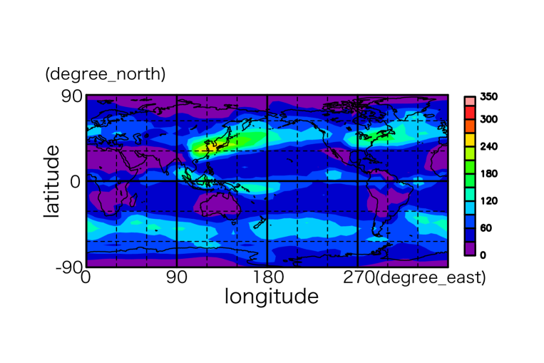
Figure 4 shows the annual mean cloud column density distribution of planets with different obliquities. Results for 30∘ show the cloud belts on the equator and mid-latitudes. The clouds around the equator are generated by the Hadley circulation. This circulation also produces subtropical highs, which are shown as the partially cloudless continents around the latitude .
The cloud patterns for and are very similar to those for and , respectively. This is due to the symmetry with respect to the stellar location for the cases of and . The results for and have the different cloud patterns due to their atmospheric circulation from the day-side pole to the equator. The present result is roughly consistent with that shown in Williams & Pollard (2003), but quantitative comparison is beyond the scope of this paper. As we mentioned earlier, however, the precise modeling of the climate is not the focus of this work. We plan to make further comparison elsewhere.
2.3 Simulated lightcurves
2.3.1 Scattering model and radiative transfer through the planetary atmosphere
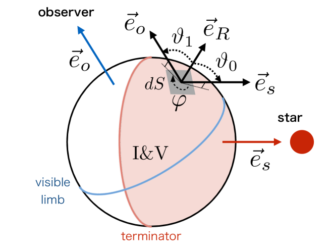
The total flux of the scattered light from the planet at wavelength is computed by integrating the intensities over the illuminated(I) and visible(V) region of the planetary surface:
| (3) |
where is the projected area element of the planetary surface viewed by the observer located at a distance of .
The location of each planetary surface area element is specified by the three angles (, and ) as illustrated in Figure 5. Then the intensity from the planetary surface area element is given by
| (4) |
where is the incident flux and is the BRDF (bi-directional reflectance distribution function) that characterizes the scattering properties of the planetary surface.
Because includes the entire radiative effects of atmosphere, clouds and solid/liquid planetary surface, we need to perform a numerical radiative transfer calculation through the planetary atmosphere. For that purpose, we compute using a public code libRadtran (Emde et al., 2016; Mayer & Kylling, 2005), which solved the radiative transfer based on various detailed models of optical properties of Earth’s atmosphere, clouds, aerosols, lands, and ocean 555We use the libRadtran version 2.0.1. URL:http://www.libradtran.org/doku.php.
The libRadtran provides several different options for specific models. We choose the following options.
-
1.
We choose REPTRAN (Gasteiger et al., 2014) for optical properties of the planetary atmosphere.
-
2.
We compute optical properties of clouds according to Hu & Stamnes (1993). We adopt 10 m for the effective radius of water cloud particles, as assumed in our GCM simulation.
-
3.
We select the Ross-Li BRDF model (Wanner et al., 1995) for land scattering. We adopt three Ross-Li parameters that are required to provide in libRadtran from a remote sensing project of the Earth, MODIS (MODerate resolution Imaging Spectroradiometer; Salomonson et al., 1989). More specifically, we choose their data set “snow-free gap-filled MODIS BRDF Model Parameters”. In doing so, we employ the data in March, neglecting the annual variation. Also, we sample the three parameters at the center of each grid on the planetary surface (), instead of averaging over the entire grid. We adopt the above approximation just for simplicity.
-
4.
Since the above particular data set does not have sufficient information for Antarctica, we assume the Lambert scattering and employ the ice albedos of (0.948, 0.921, 0.891, 0.837, 0.562, 0.233), corresponding to the six MODIS bands from 1 to 6 described below. These values of ice albedo is picked from the data “snow-free gap-filled MODIS BRDF Model Parameters” at (N69∘.20, W39∘.35). This approximation is not serious because the ice albedos do not change so much depending on the area.
- 5.
-
6.
Finally, we solve the radiative transfer equation through the atmosphere under a plane parallel approximation. We choose DISORT (DIScrete-Ordinate-method Radiative Transfer model; Stamnes et al., 1988).
We use the GCM output of water cloud density, ice cloud density, temperature, air density, and vapor mixing ratio as the input vertical profiles of atmosphere and clouds for libRadtran. While our GCM simulations distinguish between ice cloud and water cloud, we regard the ice cloud as water cloud in libRadtran so as to reduce the computational cost. For simplicity, we ignore the radiative transfer outside the region of GCM simulation ( 0-30 km), including effects due to the upper atmosphere of the planet, exo-zodiacal dust and the interstellar medium.
We compute the intensity in six photometric bands centered at the wavelengths of the MODIS bands (Table 1) but with an expanded bandwidth of m.
| band number | MODIS central wavelength |
|---|---|
| 1 | 0.469 m |
| 2 | 0.555 m |
| 3 | 0.645 m |
| 4 | 0.858 m |
| 5 | 1.240 m |
| 6 | 1.640 m |
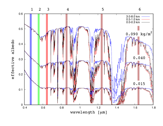
The MODIS project selected their photometric bands so as to characterize the reflection properties of the Earth’s surface by remote sensing. Figure 6a shows examples of effective albedo (reflectance) spectrum for different components of the Earth’s surface; soil, vegetation, and ocean. Three bands (1-3) roughly correspond to the visible color of blue, green, and red, respectively. Figure 6a exhibits a clear difference among the three components, ocean, soil, and vegetation. Incidentally, the MODIS project chooses 3 near-IR bands that correspond to observational windows of Earth’s atmosphere (Figure 6b).
As we have already emphasized, the cloud distribution is the most important ingredient in our mock simulation. In order to examine the dependence on their properties, we generate a simple cloud distribution as follows. Our GCM result for indicates that the simulated cloud distribution has typical column densities of kg/m2. Thus we redistribute all the clouds homogeneously within 0.0-0.3, 0.5-1.0, and 3.0-8.0 km, which roughly correspond to the typical heights for mist, lower clouds, and middle clouds for the Earth.
Figure 7 shows the resulting effective albedos for those mock clouds, indicating that the albedos are mainly determined by the column density, and fairly insensitive to the height of clouds.
2.3.2 Simulated images and lightcurves of an Earth-twin
Before performing the frequency modulation analysis, let us present examples of the apparent images and lightcurves from our mock observation.
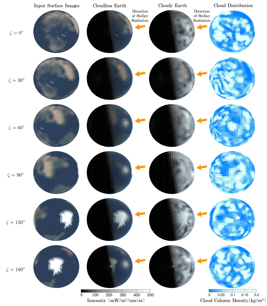
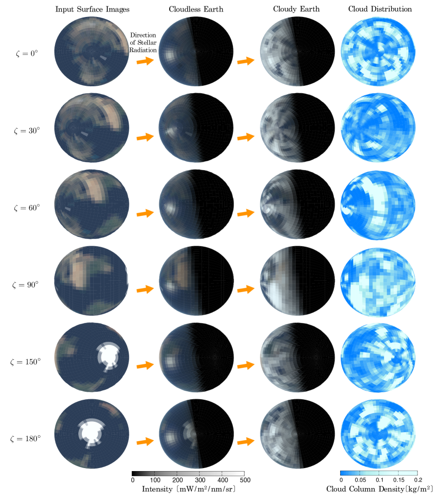
Figures 8a and 8b show the images of an Earth-twin in January and July, respectively, with different obliquities viewed from a distant observer at . Plotted from left to right are input surface distribution, illuminated and visible part of the cloudless earth with atmosphere, illuminated and visible part of the earth with both cloud and atmosphere from our GCM simulation, and the corresponding cloud distribution. The arrows indicate the incident direction of the starlight.
The input surface distribution (the left images) is computed from the intensity of land alone, neglecting the contribution of the ocean reflection. The land is assumed to be covered by the US Standard Atmosphere (Anderson, 1986) and land scattering is approximated by Lambertian. Since those images are just for reference, we assume the geometric configuration with .
The different surface components are illustrated in orange, green and blue for continents, vegetation and oceans, respectively. In the left images, one may identify North and South America, Eurasia, Africa, and Antarctica. The images of the cloudless earth relatively well exhibit colors of surface below atmosphere, and also show an oceanic glint (oceanic mirror reflection) in the illuminating direction(Sagan et al., 1993; Robinson et al., 2010). Those signatures of the surface components are significantly degraded by the clouds, but one may still identify the presence of the Sahara desert for in Figure 8a, for instance. Although one may not identify the Sahara desert for in January (Figure 8a), the Sahara desert appears in the visible and illuminating part in July (Figure 8b). Thus it can be still used a frequency modulation indicator partially in a year.
Figures 8a and 8b reconfirm that the cloud distribution weakens the surface information in photometric monitoring, but still indicate that the diurnal variation and possibly its frequency modulation detection are feasible if there exists a good tracer of the global planetary surface like the Sahara desert.
Mock photometric monitoring of the images presented in Figures 8a and 8b generates the corresponding simulated lightcurves. Throughout the analysis in what follows, we consider an observer located at for simplicity. Since we output results of our GCM simulations every three hours, we construct simulated lightcurves from those discrete snapshots. Then we ignore the change of the lightcurve during the three hours, and construct mock lightcurves sampled every three hours. While this approximate method significantly affects the lightcurve variation on a time-scale less than three hours, the variation around a planetary spin period (24 hours) of our interest is hardly affected.
Figure 9 shows an example of one-week lightcurves in January for Earth-twins with different obliquities; left and right panels correspond to those in band 1 and 4, respectively. We assume that the star-planet system is located at a distance away from the telescope of diameter and exposure time of . In an idealized case where both the light from the host star and other instrumental noises are completely neglected, the photon counts at band with the bandwidth of are scaled as
| (5) |
The photon counts in Figure 9 correspond to (left panel) and (right panel) for the bands 1 and 4 in equation (5). In practice, we compute from snapshots every three hours, assuming hours.
The simulated lightcurves for 60∘ exhibit a kind of diurnal periodicity, which does not reflect the surface information directly, but comes mainly from the cloud pattern correlated with the surface distribution. As increases (), the diurnal periodicity is not easy to identify. As we mentioned in the above, the Sahara desert played an important role as a tracer of the planetary rotation, and the annual-averaged cloud pattern is also correlated to the distribution of the surface components. This is why the diurnal periodicity is more visible for photometric monitoring of the Northern Hemisphere in the case of the Earth. Although in case of , the north part of the South America takes the role as well, it eventually sets out of visible and illuminated region as increases.
3 Time-frequency analysis of simulated lightcurves and parameter estimation
Given the simulated lightcurves, we perform the frequency modulation analysis following K16. In practice, we use a numerical code juwvid to compute the pseudo-Wigner distribution, which is publicly available from the web site666https://github.com/HajimeKawahara/juwvid.
Our time-frequency analysis proceeds as follows. First we compute from our simulated lightcurves every three hours over an orbital period of one year. Then we sample from the Poisson distribution with the expectation value of . In other words, we consider the shot noise alone in the analysis below. In total, we have (=1 year/3hours) data points, and duplicate the data points with the period of 1 year.
We divide each lightcurve into 73 segments consisting of 40 consecutive data points (i.e., 3 hours 40 5 days). Then we compute the mean and standard deviation of in each segment, and convert to the normalized lightcurve . Finally we compute the pseudo-Wigner distribution:
| (6) |
where
| (7) |
is the analytic signal of with being the Fourier transform of the normalized lightcurve in the present case. We choose the window function as the following Hamming window function:
| (10) |
In practice, we adopt year for the the window width of the Hamming window function.
The pseudo-Wigner distribution is an appropriate time-frequency distribution for extracting the instantaneous frequency (e.g. Cohen, 1995), as explained below. Let us consider a single mode signal with an instantaneous phase , where is the amplitude of the mode. The ideal time-frequency representation is a delta function , where is the instantaneous frequency defined by
| (11) |
Then, the inverse Fourier transform of can be written as
| (12) |
where we use the linear approximation in the last two terms.
Performing the Fourier transform of equation (12) with the time window, we obtain the pseudo-Wigner distribution. Because the linear approximation is valid only for the linear frequency modulation such as ( are constant values), the width of the window should be chosen to be comparable to the scale of the non-linear feature of the frequency modulation. The derivative of equation (12) by at provides
| (13) |
Also, the mode amplitude is rewritten as
| (14) |
Then, the instantaneous frequency is formally estimated by the weighted form as,
| (15) |
In practice, one can estimate the peak value of the pseudo-Wigner distribution as an instantaneous frequency to avoid the effect of noise. In this expression, we need a complex-valued signal with non-negative frequency component of the signal. That is the reason why we convert a real-valued signal to the analytic signal in equation (7).
We calculate the pseudo-Wigner distribution over the range of using equation (6). Specifically we choose [day-1] and [day-1] throughout the analysis. Since our lightcurves are sampled every 3 hours, the corresponding frequency resolution is not good enough to determine the value of precisely. Therefore we adopt a non-uniform FFT scheme (Greengard & Lee, 2004) following K16, and achieved the frequency resolution of after applying an appropriate smoothing of the lightcurves. We choose in what follows, and the resulting resolution [day-1] is better than the modulation amplitude detected in Figure 16 by a factor of 100.
3.1 Single-band analysis
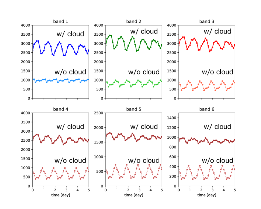
Consider first the frequency modulation for single-band lightcurves. Figure 11 is similar to Figure 9, but plots simulated noiseless (without shot noise) lightcurves in the photometric bands 1 to 6 for .
As clearly indicated by Figure 11, the apparent diurnal variation in each band originates from the cloud pattern that is correlated with the land-ocean distribution. These surface-correlated clouds were also found in Earth observations by Deep Space Climate Observatory as the second component of the Principal Component Analysis (Fan et al., 2019). While our analysis did not directly identify the component, it appears to be imprinted in the diurnal variation in a single band. The amplitude of the single-band lightcurves is basically determined by the cloud albedo (Figure 7) multiplied by the incident solar flux. This is why the amplitude of the diurnal variation with cloud in Figure 11 is relatively large around the visible wavelength (bands 2 and 3), and declines sharply in the near-infrared (bands 4 to 6).
We note that Figure 11 also indicates the anti-correlation of the lightcurve modulation between cloudless and cloudy cases. For a cloudless case, the photometric variation is mainly due to the land component that has larger albedos (Figures 6a and Figure 7). Since clouds are much brighter, however, the photometric variation of a cloudy case is sensitive to the location of clouds, which tend to avoid the continent, in particular desert regions, and rather form preferentially above the ocean. Thus the locations of lands and clouds are anti-correlated, leading to the anti-correlation illustrated in Figure 11. This also explains that the periodic signature of the lightcurve for a cloudy case is weaker for redder bands, because lands become brighter in redder bands and compensate the variation due to clouds.
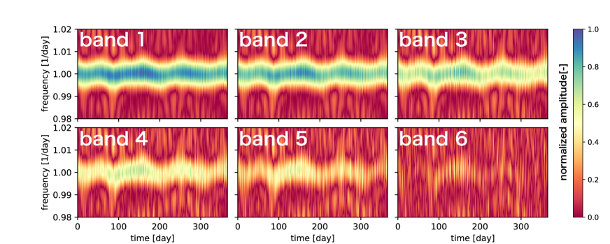
The corresponding color-map for the pseudo-Wigner distribution on the time-frequency plane (Figure 11) clearly illustrates the above trend that redder bands have weaker signal. The color indicates the absolute value of the time-frequency distribution density , whose maximum value is normalized as unity. Since Figure 11 is for , the period for the apparent diurnal variation should be constant, and does not show any frequency modulation. The tiny frequency modulation day-1 visible in Figure 11 is simply due to the time-dependent inhomogeneous distribution of clouds.
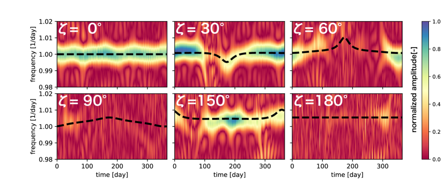
Consider next the time-frequency representation of the band-1 lightcurves for different obliquities (Figure 12). We adopt band 1 because it produces the clearest ridge on time-frequency representation in Figure 11. The dashed lines show the model frequency modulation , equation (1). The signature of the frequency modulation from the single-band lightcurves is not strong, and barely identifiable only for . Though the amplitude of frequency modulation is zero for , the signature of the constant apparent frequency is visible clearly. This obliquity dependence reflects the specific distribution pattern of land and ocean on the Earth. As shown in the image in Figure 8a, the illuminated and visible part in winter is dominated by Antarctica, and there is no significant diurnal variation in the lightcurve. On the other hand, in summer, Antarctica is almost invisible and parts of Africa and South America generate the diurnal variation signal instead.
3.2 Multi-band analysis
As shown in Section 3.1, single-band analysis does not properly extract the information of the correct frequency modulation due to the anti-correlation between lands and clouds. In order to detect the diurnal period due to the planetary surface distribution, therefore, we need to remove the time-dependent cloud pattern as much as possible.
As inferred from the wavelength dependence of albedos for lands and clouds, bands 1 and 4 are mainly sensitive to clouds and cloudslands, respectively (see Figure 6a and Figure 7). Thus the difference of the photon counts and roughly removes the contribution from clouds.
For definiteness, we choose the following linear combination of bands 1 and 4:
| (16) | |||||
| (17) |
The above combination is derived assuming that the albedo of clouds is roughly independent of the wavelength, and thus the contribution of the clouds is canceled, at least partially as shown in Figure 13. While the cloud effect may be removed more efficiently by combining other bands appropriately, it is beyond the scope of the present paper. Thus we perform the frequency modulation analysis using equation (16) in what follows.
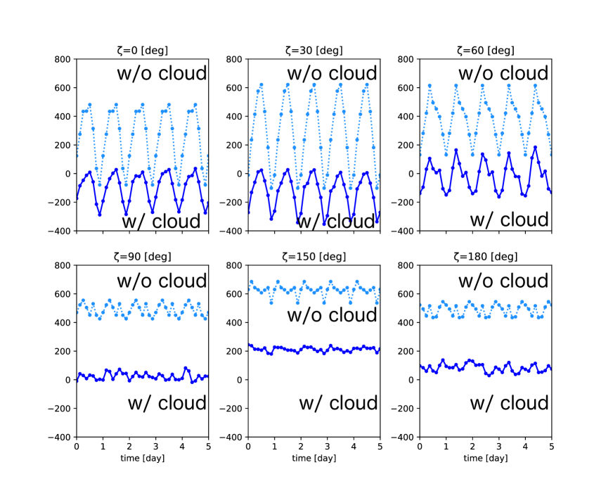
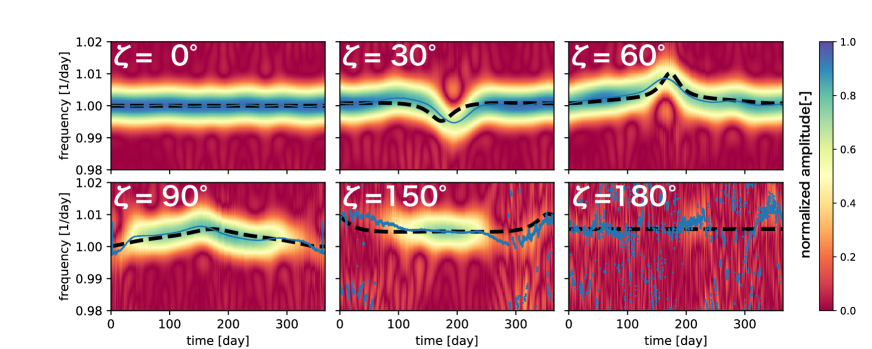
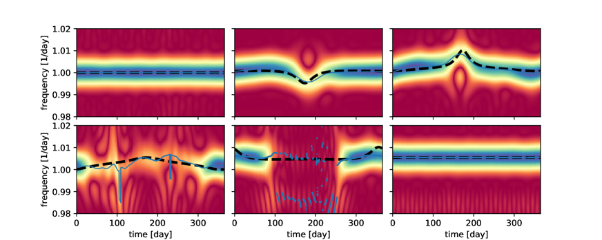
Figure 13 shows an example of simulated noiseless lightcurves using , and Figure 14 is the corresponding time-frequency representation. Comparison between Figures 12 and 14 clearly indicates that the multi-band analysis suppresses the time-dependent cloud effect, and significantly improves the frequency modulation signal.
We note that the amplitude of the frequency modulation signature depicted in Figure 14 sensitively depends on the value of , reflecting the specific surface distribution on the Earth. As indicated in Figures 8a and 8b, the Southern Hemisphere, especially around the South Pole, of the Earth is occupied by Antarctica and ocean, in an approximately axisymmetric manner. Thus the diurnal variation of the Southern Hemisphere (for example, viewed from the direction of if ) is difficult to detect. This also applies to the case in which the frequency modulation signal is clear only in summer, as described at the end of subsection 3.1.
In contrast, the Northern Hemisphere is roughly divided into two major distinct components; the Eurasian continent and the Pacific ocean. This large-scale inhomogeneity, in particular the Sahara desert, acts as a good tracer of an asymmetric surface pattern, yielding a relatively large amplitude signal of the frequency modulation (see Figures 8a and 8b). This is why a clear frequency modulation signal in the case of can be detected for an observer located at .
3.3 Feasibility of the obliquity estimate
All of the pseudo-Wigner distributions above (Figures 11, 12, and 14) are based on noiseless data. Now we are in a position to examine to what extent one can estimate the planetary obliquity from the long-term photometric monitoring via the frequency modulation method. For that purpose, we assume a dedicated space mission with the telescope aperture of , 4 and 6 m. Again we consider idealized cases in which the photometric noise comes from the photon shot-noise alone, and generate a set of lightcurves from the photon counts and obeying the Poisson statistics. Examples of the resulting frequency modulation are presented in Figure 15.
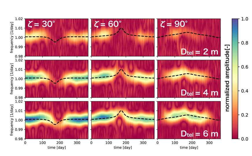
The model frequency modulation is determined by the five parameters (, , , , ) that are listed in Table 2; the planetary obliquity , the planetary spin frequency , the angle of the vernal equinox measured from the location of the observer projected on the orbital plane , the observer’s inclination , and the orbital frequency of the planet . Among them, and simply specify the location of the observer relative to the system, and are not so interesting. The remaining three parameters, , and , are important since they characterize the star-planet system.
In order to estimate , which cannot be estimated otherwise and thus are of our primary interest, we need to perform eventually a joint analysis of the five parameters in a Bayesian fashion. In the present study, however, we would like to examine the feasibility of the determination of and , assuming that and are known, for simplicity. The precise spectroscopic and astrometric data would determine and . Also, may be estimated from the photometric data on relatively short-time scales apart from the uncertainty of in equation (1).
Under the similar assumption, K16 attempted to find the best-fit values for , , and by minimizing
| (18) |
where is the frequency derived from the maximum-weighted longitude approximation, equation (1), and corresponds to the maximum value of over a range of at each epoch . We tried the same fitting, but the result is not robust against the shot noise especially when the frequency modulation signal is weak.
Therefore we empirically improve the fit by taking account of the distribution around the as well. More specifically, we construct a Gaussian weighted model for the time-frequency distribution:
| (19) |
where is a new fitting parameter that is introduced to account for the finite width of the frequency distribution around .
Then we minimize the following quantity:
| (20) |
to find the best-fit , , , and . The value of should be roughly equal to because the time-frequency representation of a signal based on the pseudo-Wigner distribution has a dispersion corresponding to the Fourier transform of the window function , and this dispersion is flattened due to the noise and non-linear frequency modulation.
In practice, we use the Levenberg-Marquardt algorithm mpfit(Markwardt, 2009) to find the best-fit parameters. This algorithm is a practical and fast algorithm of the least square method for non-linear functions. We fit the time-frequency distribution for and . Table 2 summarizes our initial parameters in addition to the fixed orbital parameters that we assume to be a priori known.
| Initial parameter | value |
|---|---|
| obliquity | 15 () |
| () | |
| spin frequency | 366 [year-1] |
| Fixed parameter | value |
| orbital inclination | 0∘ |
| orbital frequency | 1 [year-1] |
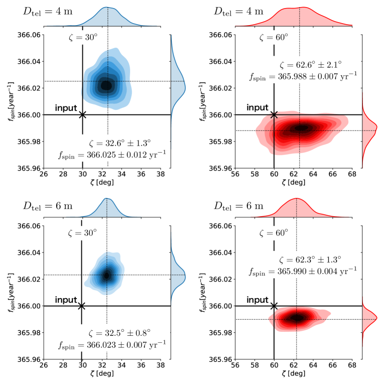
Figure 16 shows the distribution of the best-fit estimates on the - plane from 1000 different realizations. The black cross symbols indicate the input values, ( ) = (, 366 year-1) and (, 366 year-1), for left and right panels, respectively. The top and bottom panels show the results based on the shot-noise limited observations with 4 m and 6 m, respectively. The numbers in each panel denote the mean and 1 estimated from 1000 realizations.
The systematic offsets of and year-1 result most likely from the specific pattern of the continents on the Earth. Indeed the previous simplified analysis by K16 also found a similar level of the systematic offset of the planetary obliquity ( several degrees; see Figure 8 of K16). K16 added noises empirically into his mock data, neglecting the time-dependent cloud distribution that we compute here.
The fact that the systematic offsets between the two analyses are similar indicates, therefore, that they should be ascribed to the specific surface pattern of the Earth itself. Indeed Eurasia, North Africa, and South America are distributed roughly from northeast to southwest directions. This latitudinal pattern is consistent with the positive systematic offset of the obliquity exhibited in Figure 16. Since the amplitude of the systematic offset would depend on the specific pattern of the planetary surface to some extent, it is difficult to predict it a prior, but important to bear in mind that it could amount to several degrees, much larger than the statistical uncertainty as shown in Figure 16.
4 Summary and conclusion
The direct imaging of earth-like planets is very challenging, but will provide ground-breaking datasets for astronomy, planetary science, and biology, if successful eventually. One notable example is the reconstruction of the surface components (e.g., Sagan et al., 1993; Ford et al., 2001; Fujii et al., 2010, 2011; Kawahara & Fujii, 2011; Fujii & Kawahara, 2012; Suto, 2019), and it may be even possible to measure the planetary obliquity through the frequency modulation of the photometric lightcurve of future direct imaged Earth-like planets, proposed by Kawahara (2016).
We have examined the feasibility of the methodology by creating simulated lightcurves of our Earth-Sun systems but with different planetary obliquities. First, we performed the GCM simulation for those systems with particular emphasis on the time-dependent cloud distribution. Second, we computed the scattered light in 6 photometric bands by solving the radiation transfer of the incident starlight through the cloud and atmosphere taking into account the scattering due to the different surface components under the parameterized bi-directional reflectance distribution function models (Wanner et al., 1995; Nakajima, 1983). Third, the resulting light from the planet was mock-observed every three hours over the orbital period of one year, and simulated lightcurves were constructed by combining the different photometric bands so as to suppress the effect of the time-dependent cloud pattern. Finally, we computed the frequency modulation of the lightcurves using the pseudo-Wigner distribution and attempted to estimate the planetary obliquities for photon-shot noise dominated cases.
We found that the frequency modulation signal is crucially dependent on the presence of the large-scale inhomogeneity on the planetary surface. Indeed this is the case for the Northern Hemisphere of our Earth; in particular the Sahara desert turned out to be a useful tracer of the planetary spin rotation. The Southern Hemisphere, on the other hand, is relatively featureless, and the frequency modulation signal is weak.
As a result, we found that a dedicated 4 m space telescope at 10 pc away from the system in the face-on view relative to the observer can estimate the planetary obliquity within the uncertainty of several degrees in principle (in the shot-noise limited case). Although this conclusion is based on several idealized assumptions at this point, we believe that it is very encouraging for the future exploration of the direct imaging of Earth-like planets.
Appendix A Behavior of the frequency modulation factor for an eccentric orbit
The modulation factor, equation (2), first derived by K16 assumes a circular orbit for simplicity. We compute a generalized expression for an eccentric orbit, and present the effect of eccentricity on the frequency modulation based on the maximum weighted longitude approximation.
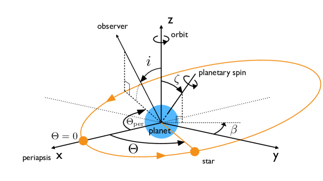
For an eccentric orbit, it is more convenient to consider a geocentric frame where the -axis is the direction toward the periapsis as shown in Figure 17, instead of vernal equinox (c.f., Figure 3). In this frame, the spin vector is no longer on the -plane, and we introduce a new parameter , which denotes the azimuthal angle of the planetary spin measured from -axis. Similarly the location of the observer is specified by the phase angle from the periapsis , and is now the azimuthal angle measured clockwise from the periapsis, i.e., the true anomaly. The frame reduces to that shown in Figure 3 for , , , and .
Following K16, we assume that the longitude of the reflective point on the planetary surface, , traces faithfully the observable periodicity of the planetary scattered light. Then the observed frequency is given in terms of as
| (A1) | |||||
| (A2) |
where
| (A3) | |||||
| (A4) | |||||
| (A5) |
For a circular orbit, is equal to . For , however, it cannot be written explicitly in terms of , but is expressed as
| (A6) |
In the geocentric frame, unit vectors toward the star and the observer, and , are given as , and , respectively. Thus the unit vector towards the reflective point, , is
| (A10) |
where .
Consider a point on the planetary surface specified by the latitude and longitude in the rest frame of the planet. The surface normal unit vector at the point is . One can transform to in the geocentric frame as
| (A11) |
where is a spin rotation operator (), and is the rotation matrix counterclockwise around the -axis. Note that is required for a non-circular case.
We apply the generic transformation, equation (A11), to compute the component of the reflective point in the planetary frame. Then we obtain
| (A12) | |||||
| (A16) |
The ratio of the - and -components in equation (A12) yields
| (A17) |
Therefore equation (A3) reduces to
| (A18) |
Finally we obtain the eccentric frequency modulation in terms of true anomaly :
| (A19) |
The above equation reproduces equation (2) for , , , and .
In the main part of the paper, we consider the circular orbit alone just for simplicity, but the effect of is important as well. To show this, we plot equation A19 for the Earth-like planet viewed from for and in Figure 18. The horizontal axis indicates the time in units of that is numerically computed from the true anomaly. The left and right panels correspond to the obliquity of and . Different curves indicate cases for , , , and .
The dashed () and solid () clearly exhibit different amplitudes and phases of the frequency modulation. Thus the effect of eccentricity biases the estimates of and if the formula for is used in fitting the data. Since it is likely that the orbit of direct imaging targets is precisely determined prior to its monitoring, one can use equation (A19) as a template using the estimated value of .
References
- Aizawa et al. (2020) Aizawa, M., Kawahara, H., & Fan, S. 2020, arXiv e-prints, arXiv:2004.03941. https://arxiv.org/abs/2004.03941
- Anderson (1986) Anderson, G. P. 1986, AFGL atmospheric constituent profiles (0-120km)
- Beljaars (1995) Beljaars, A. C. M. 1995, Quarterly Journal of the Royal Meteorological Society, 121, 255
- Beljaars & Holtslag (1991) Beljaars, A. C. M., & Holtslag, A. A. M. 1991, Journal of Applied Meteorology, 30, 327
- Cohen (1995) Cohen, L. 1995, Time-frequency analysis, Prentice Hall signal processing series (Prentice Hall PTR). http://ci.nii.ac.jp/ncid/BA25293241
- Cowan et al. (2009) Cowan, N. B., Agol, E., Meadows, V. S., et al. 2009, ApJ, 700, 915
- Deitrick et al. (2018) Deitrick, R., Barnes, R., Bitz, C., et al. 2018, AJ, 155, 266
- Emde et al. (2016) Emde, C., Buras-Schnell, R., Kylling, A., et al. 2016, Geoscientific Model Development, 9, 1647
- Fan et al. (2019) Fan, S., Li, C., Li, J.-Z., et al. 2019, ApJ, 882, L1
- Farr et al. (2018) Farr, B., Farr, W. M., Cowan, N. B., Haggard, H. M., & Robinson, T. 2018, AJ, 156, 146
- Ford et al. (2001) Ford, E. B., Seager, S., & Turner, E. L. 2001, Nature, 412, 885
- Fujii & Kawahara (2012) Fujii, Y., & Kawahara, H. 2012, ApJ, 755, 101
- Fujii et al. (2011) Fujii, Y., Kawahara, H., Suto, Y., et al. 2011, ApJ, 738, 184
- Fujii et al. (2010) —. 2010, ApJ, 715, 866
- Gasteiger et al. (2014) Gasteiger, J., Emde, C., Mayer, B., et al. 2014, J. Quant. Spec. Radiat. Transf., 148, 99
- Greengard & Lee (2004) Greengard, L., & Lee, J.-Y. 2004, SIAM Review, 46, 443
- Hu & Stamnes (1993) Hu, Y. X., & Stamnes, K. 1993, Journal of Climate, 6, 728
- Jiang et al. (2018) Jiang, J. H., Zhai, A. J., Herman, J., et al. 2018, AJ, 156, 26
- Kaspi & Showman (2015) Kaspi, Y., & Showman, A. P. 2015, ApJ, 804, 60
- Kawahara (2016) Kawahara, H. 2016, ApJ, 822, 112
- Kawahara & Fujii (2010) Kawahara, H., & Fujii, Y. 2010, ApJ, 720, 1333
- Kawahara & Fujii (2011) —. 2011, ApJ, 739, L62
- Komacek et al. (2019) Komacek, T. D., Jansen, M. F., Wolf, E. T., & Abbot, D. S. 2019, ApJ, 883, 46
- Le Treut & Li (1991) Le Treut, H., & Li, Z.-X. 1991, Climate Dynamics, 5, 175
- Manabe (1969) Manabe, S. 1969, Monthly Weather Review, 97, 739
- Markwardt (2009) Markwardt, C. B. 2009, in Astronomical Society of the Pacific Conference Series, Vol. 411, Astronomical Data Analysis Software and Systems XVIII, ed. D. A. Bohlender, D. Durand, & P. Dowler, 251. https://arxiv.org/abs/0902.2850
- Mayer & Kylling (2005) Mayer, B., & Kylling, A. 2005, Atmospheric Chemistry and Physics, 5, 1855
- Mellor & Yamada (1982) Mellor, G. L., & Yamada, T. 1982, Reviews of Geophysics and Space Physics, 20, 851
- Moorthi & Suarez (1992) Moorthi, S., & Suarez, M. J. 1992, Monthly Weather Review, 120, 978
- Nakajima (1983) Nakajima, T. 1983, J. Quant. Spec. Radiat. Transf., 29, 521
- Noda et al. (2017) Noda, S., Ishiwatari, M., Nakajima, K., Takahashi, Y. O., Takehiro, S., Onishi, M., Hashimoto, G. L., Kuramoto, K., & Hayashi, Y.-Y., 2017, Icarus, 282, 1
- Oakley & Cash (2009) Oakley, P. H. H., & Cash, W. 2009, ApJ, 700, 1428
- Pallé et al. (2008) Pallé, E., Ford, E. B., Seager, S., Montañés-Rodríguez, P., & Vazquez, M. 2008, ApJ, 676, 1319
- Robinson et al. (2010) Robinson, T. D., Meadows, V. S., & Crisp, D. 2010, ApJ, 721, L67
- Rose (2015) Rose, B. E. J. 2015, Journal of Geophysical Research: Atmospheres, 120, 1404
- Rushby et al. (2019) Rushby, A. J., Shields, A. L., & Joshi, M. 2019, ApJ, 887, 29
- Sagan et al. (1993) Sagan, C., Thompson, W. R., Carlson, R., Gurnett, D., & Hord, C. 1993, Nature, 365, 715
- Salomonson et al. (1989) Salomonson, V. V., Barnes, W. L., Maymon, P. W., Montgomery, H. E., & Ostrow, H. 1989, IEEE Transactions on Geoscience and Remote Sensing, 27, 145
- Schwartz et al. (2016) Schwartz, J. C., Sekowski, C., Haggard, H. M., Pallé, E., & Cowan, N. B. 2016, MNRAS, 457, 926
- Stamnes et al. (1988) Stamnes, K., Tsay, S.-C., Jayaweera, K., & Wiscombe, W. 1988, Appl. Opt., 27, 2502
- Suto (2019) Suto, Y. 2019, How to Search for Possible Bio-signatures on Earth-Like Planets: Beyond a Pale Blue Dot, ed. A. Yamagishi, T. Kakegawa, & T. Usui, 441
- Wanner et al. (1995) Wanner, W., Li, X., & Strahler, A. H. 1995, Journal of Geophysical Research: Atmospheres, 100, 21077
- Williams & Pollard (2003) Williams, D. M., & Pollard, D. 2003, International Journal of Astrobiology, 2, 1