Two regularized energy-preserving finite difference methods for the logarithmic Klein-Gordon equation

Jingye Yan yanjingye0205@163.com Xu Qian qianxu@nudt.edu.cn Hong Zhang zhanghnudt@163.com Songhe Song shsong@nudt.edu.cn Department of Mathematics, College of Arts and Sciences, National University of Defense Technology, Changsha 410073, China Department of Mathematics, National University of Singapore, Singapore 119076 State Key Laboratory of High Performance Computing, National University of Defense Technology, Changsha 410073, China
Abstract

We present and analyze two regularized finite difference methods which preserve energy of the logarithmic Klein-Gordon equation (LogKGE). In order to avoid singularity caused by the logarithmic nonlinearity of the LogKGE, we propose a regularized logarithmic Klein-Gordon equation (RLogKGE) with a small regulation parameter 0<ε10𝜀much-less-than10<\varepsilon\ll 1 to approximate the LogKGE with the convergence order O(ε)𝑂𝜀O(\varepsilon). By adopting the energy method, the inverse inequality, and the cut-off technique of the nonlinearity to bound the numerical solution, the error bound O(h2+τ2ε2)𝑂superscript2superscript𝜏2superscript𝜀2O(h^{2}+\frac{\tau^{2}}{\varepsilon^{2}}) of the two schemes with the mesh size hh, the time step τ𝜏\tau and the parameter ε𝜀\varepsilon. Numerical results are reported to support our conclusions.

keywords:
logarithmic Klein-Gordon equation; regularized logarithmic Klein-Gordon equation; finite difference method; error estimate; convergence order; energy-preserving

1 Introduction

Consider the Klein-Gordon equation with the logarithmic nonlinear term (LogKGE),

{utt(𝐱,t)Δu(𝐱,t)+u(𝐱,t)+λu(𝐱,t)ln(|u(𝐱,t)|2)=0,𝐱Ω,t>0,u(𝐱,0)=ϕ(𝐱),tu(𝐱,0)=γ(𝐱),𝐱Ω¯,\displaystyle\left\{\begin{aligned} &u_{tt}(\mathbf{x},t)-\Delta u(\mathbf{x},t)+u(\mathbf{x},t)+\lambda u(\mathbf{x},t)\ln(|u(\mathbf{x},t)|^{2})=0,~{}~{}\mathbf{x}\in\Omega,t>0,\\ &u(\mathbf{x},0)=\phi(\mathbf{x}),~{}~{}~{}\partial_{t}u(\mathbf{x},0)=\gamma(\mathbf{x}),~{}~{}~{}\mathbf{x}\in\overline{\Omega},\end{aligned}\right. (1.1)

where 𝐱=(x1,,xd)Td,(d=1,2,3)formulae-sequence𝐱superscriptsubscript𝑥1subscript𝑥𝑑Tsuperscript𝑑𝑑123\mathbf{x}=(x_{1},\ldots,x_{d})^{\mathrm{T}}\in\mathbb{R}^{d},(d=1,2,3) is the spatial coordinate, t𝑡t is time, u:=u(𝐱,t)assign𝑢𝑢𝐱𝑡u:=u(\mathbf{x},t) is a real-valued scalar field, the parameter λ𝜆\lambda measures the force of the nonlinear interaction and Ω=dΩsuperscript𝑑\Omega=\mathbb{R}^{d} or ΩdΩsuperscript𝑑\Omega\subset\mathbb{R}^{d} is a bounded domain with homogeneous Dirichlet or periodic boundary condition fixed on the boundary.

The LogKGE (1.1) is a relativistic version of the logarithmic Schrödinger equation [1] which was introduced by Rosen [2] in the quantum field theory. Such kinds of nonlinearity arise from different applications, such as optics [3], nuclear physics [4, 5] , supersymmetric field theories [2], inflation cosmology [6, 7], and geophysics [8] to describe the spinless particle [9].

Similar to the nonlinear Klein-Gordon equation (NKGE),

{utt(𝐱,t)Δu(𝐱,t)+u(𝐱,t)+u(𝐱,t)3=0,𝐱Ω,t>0,u(𝐱,0)=ϕ(𝐱),tu(𝐱,0)=γ(𝐱),𝐱Ω¯,\displaystyle\left\{\begin{aligned} &u_{tt}(\mathbf{x},t)-\Delta u(\mathbf{x},t)+u(\mathbf{x},t)+u(\mathbf{x},t)^{3}=0,~{}~{}\mathbf{x}\in\Omega,t>0,\\ &u(\mathbf{x},0)=\phi(\mathbf{x}),~{}~{}~{}\partial_{t}u(\mathbf{x},0)=\gamma(\mathbf{x}),~{}~{}~{}\mathbf{x}\in\overline{\Omega},\end{aligned}\right. (1.2)

the LogKGE (1.1) admits the energy conservation law [10, 11], which is defined as:

E(t)=Ω[(ut(𝐱,t))2+(u(𝐱,t))2+(1λ)u2(𝐱,t)+λu2(𝐱,t)ln(|u(𝐱,t)|2)]d𝐱E(0),𝐸𝑡subscriptΩdelimited-[]superscriptsubscript𝑢𝑡𝐱𝑡2superscript𝑢𝐱𝑡21𝜆superscript𝑢2𝐱𝑡𝜆superscript𝑢2𝐱𝑡superscript𝑢𝐱𝑡2differential-d𝐱𝐸0\displaystyle E(t)=\int_{\Omega}\left[(u_{t}(\mathbf{x},t))^{2}+(\nabla u(\mathbf{x},t))^{2}+(1-\lambda)u^{2}(\mathbf{x},t)+\lambda u^{2}(\mathbf{x},t)\ln\left(|u(\mathbf{x},t)|^{2}\right)\right]\mathrm{d}\mathbf{x}\equiv E(0), (1.3)

where u(,t)H1(Ω)𝑢𝑡superscript𝐻1Ωu(\cdot,t)\in H^{1}(\Omega) and tu(,t)L2(Ω)subscript𝑡𝑢𝑡superscript𝐿2Ω\partial_{t}u(\cdot,t)\in L^{2}(\Omega).

The LogKGE (1.1) has been studied theoretically in the literature, such as the existence of some special analytical solutions in quantum mechanics [12, 13, 14], and the existence of classical solutions and weak solutions [1, 15]. In [13], the author studied the Gaussian solutions [16]. Besides, the interaction of Gaussons has been investigated in [17].

For the numerical part, different efficient and accurate numerical methods have been proposed and analyzed for computations of wave propagations in classic/relativistic physics, such as the standard finite difference time domain (FDTD) [18, 19, 20, 21, 22, 23, 24, 25] , the conservative compact finite difference method [26], the multiscale time integrator Fourier pseudospectral (MWI-FP) method [27], the finite element method [28], the time-splitting spectral method (TSFP) [29], the exponential wave integrator Fourier pseudospectral (EWI-FP) method [18, 30], the asymptotic preserving (AP) method [31], etc. Of course, each method has its advantages and disadvantages. For numerical comparisons of different numerical methods, we refer to [18, 32, 33, 34].

In the last thirty years, the conservation of invariants has draw much attention from different research fields [35, 36]. Various of conservative numerical methods have been proposed in the literature including the Crank-Nicolson finite difference (CNFD) and the semi-implicit finite difference (SIFD) [37, 24], the average vector field (AVF) method [38], the local discontinuous Galerkin methods [39], the local structure-preserving method [40], the Hamiltonian boundary value method (HBVM) [41], the Kahan method [42], etc. It is a natural question to ask whether one can design numerical methods for the LogKGE (1.1). However, these methods can not be applied and analyzed to the LogKGE (1.1) directly, because of the singularity at the origin of the logarithmic term. To our best knowledge, in [25] the authors proposed and analyzed two regularized finite difference methods for the LogKGE (1.1), but those schemes can not preserve energy. The main objective of this paper is to carry out and analyze two energy-preserving regularized finite difference methods for the LogKGE. In our numerical analysis, besides the standard techniques of the energy method, we employ the cut-off technique for dealing with the nonlinear term, and the inverse inequality for obtaining a posterior bound of the numerical solution.

The rest of this paper is organized as follows. In Section 2, a regularized version of LogKGE (1.1) with a small parameter 0<ε10𝜀much-less-than10<\varepsilon\ll 1 is proposed and we analyze the convergence of the energy between the LogKGE (1.1) and the regularized logarithmic Klein-Gordon equation (RLogKGE) (2.1). In Section 3, two energy-preserving finite difference methods are proposed for the RLogKGE, and their properties of the stability, energy convergence, solvability are also analyzed. Section 4 is devoted to establishing the details of error bounds of the two numerical methods. Numerical results are reported in Section 5 to confirm our theoretical analysis. Finally, some conclusions are drawn in Section 6. Throughout this paper, we let pqless-than-or-similar-to𝑝𝑞p\lesssim q to denote that there exists a generic constant C𝐶C which is independent of τ,h,ε𝜏𝜀\tau,h,\varepsilon, such that |p|Cq𝑝𝐶𝑞|p|\leq Cq.

2 A regularized logarithmic Klein-Gordon equation

In order to avoid blow-up and to suppress round-off error of the LogKGE (1.1), a regularized logarithmic Klein-Gordon equation (RLogKGE) with a small regulation parameter 0<ε10𝜀much-less-than10<\varepsilon\ll 1 was introduced in [25] as,

{uttε(𝐱,t)Δuε(𝐱,t)+uε(𝐱,t)+λuε(𝐱,t)ln(ε2+(uε(𝐱,t))2)=0,𝐱Ω,t>0,uε(𝐱,0)=ϕ(𝐱),tuε(𝐱,0)=γ(𝐱),𝐱Ω¯.\displaystyle\left\{\begin{aligned} &u^{\varepsilon}_{tt}(\mathbf{x},t)-\Delta u^{\varepsilon}(\mathbf{x},t)+u^{\varepsilon}(\mathbf{x},t)+\lambda u^{\varepsilon}(\mathbf{x},t)\ln\left(\varepsilon^{2}+\left(u^{\varepsilon}(\mathbf{x},t)\right)^{2}\right)=0,~{}~{}\mathbf{x}\in\Omega,t>0,\\ &u^{\varepsilon}(\mathbf{x},0)=\phi(\mathbf{x}),~{}~{}~{}\partial_{t}u^{\varepsilon}(\mathbf{x},0)=\gamma(\mathbf{x}),~{}~{}~{}\mathbf{x}\in\overline{\Omega}.\end{aligned}\right. (2.1)

The above RLogKGE (2.1) is time symmetric and time reversible, i.e., they are invarient if interchanging n+1n1𝑛1𝑛1n+1\leftrightarrow n-1 and ττ𝜏𝜏\tau\leftrightarrow-\tau.

Remark:  The regularization technique of the logarithmic term has been extensively investigated in [43]. For the Cauchy problem of the LogKGE (1.1) and the RLogKGE (2.1), the theoretical convergence estimate will be presented in our future work.

Theorem 2.1.

Assume uε(,t)H1(Ω)superscript𝑢𝜀𝑡superscript𝐻1Ωu^{\varepsilon}(\cdot,t)\in H^{1}(\Omega) and tuε(,t)L2(Ω)subscript𝑡superscript𝑢𝜀𝑡superscript𝐿2Ω\partial_{t}u^{\varepsilon}(\cdot,t)\in L^{2}(\Omega), the RLogKGE (2.1) conserves the energy , which is defined as:

Eε(t)=Ω[(utε(𝐱,t))2+(uε(𝐱,t))2+(uε(𝐱,t))2+λFε((uε(𝐱,t))2)]d𝐱Eε(0),superscript𝐸𝜀𝑡subscriptΩdelimited-[]superscriptsubscriptsuperscript𝑢𝜀𝑡𝐱𝑡2superscriptsuperscript𝑢𝜀𝐱𝑡2superscriptsuperscript𝑢𝜀𝐱𝑡2𝜆subscript𝐹𝜀superscriptsuperscript𝑢𝜀𝐱𝑡2differential-d𝐱superscript𝐸𝜀0\displaystyle E^{\varepsilon}(t)=\int_{\Omega}\left[(u^{\varepsilon}_{t}(\mathbf{x},t))^{2}+(\nabla u^{\varepsilon}(\mathbf{x},t))^{2}+(u^{\varepsilon}(\mathbf{x},t))^{2}+\lambda F_{\varepsilon}\left((u^{\varepsilon}(\mathbf{x},t))^{2}\right)\right]\mathrm{d}\mathbf{x}\equiv E^{\varepsilon}(0), (2.2)

where Fε(ρ)=0ρln(ε2+s)ds=ρln(ε2+ρ)+ε2ln(1+ρε2)ρ.subscript𝐹𝜀𝜌superscriptsubscript0𝜌superscript𝜀2𝑠differential-d𝑠𝜌superscript𝜀2𝜌superscript𝜀21𝜌superscript𝜀2𝜌F_{\varepsilon}(\rho)=\int_{0}^{\rho}\ln(\varepsilon^{2}+s)\mathrm{d}s=\rho\ln(\varepsilon^{2}+\rho)+\varepsilon^{2}\ln(1+\frac{\rho}{\varepsilon^{2}})-\rho.

Proof.
ddtEε(t)=2Ω[utεuttε+uεutε+uεutε+λFε((uε)2)uεutε](𝐱,t)d𝐱=2Ω[utε(uttεΔuε+uε+λuεln(ε2+(uε)2))](𝐱,t)d𝐱=0.dd𝑡superscript𝐸𝜀𝑡2subscriptΩdelimited-[]subscriptsuperscript𝑢𝜀𝑡subscriptsuperscript𝑢𝜀𝑡𝑡superscript𝑢𝜀subscriptsuperscript𝑢𝜀𝑡superscript𝑢𝜀subscriptsuperscript𝑢𝜀𝑡𝜆subscriptsuperscript𝐹𝜀superscriptsuperscript𝑢𝜀2superscript𝑢𝜀subscriptsuperscript𝑢𝜀𝑡𝐱𝑡differential-d𝐱2subscriptΩdelimited-[]subscriptsuperscript𝑢𝜀𝑡subscriptsuperscript𝑢𝜀𝑡𝑡Δsuperscript𝑢𝜀superscript𝑢𝜀𝜆superscript𝑢𝜀superscript𝜀2superscriptsuperscript𝑢𝜀2𝐱𝑡differential-d𝐱0\displaystyle\begin{split}\frac{\mathrm{d}}{\mathrm{d}t}E^{\varepsilon}(t)&=2\int_{\Omega}\left[u^{\varepsilon}_{t}\cdot u^{\varepsilon}_{tt}+\nabla u^{\varepsilon}\cdot\nabla u^{\varepsilon}_{t}+u^{\varepsilon}u^{\varepsilon}_{t}+\lambda F^{\prime}_{\varepsilon}\left((u^{\varepsilon})^{2}\right)\cdot u^{\varepsilon}\cdot u^{\varepsilon}_{t}\right](\mathbf{x},t)\mathrm{d}\mathbf{x}\\ &=2\int_{\Omega}\left[u^{\varepsilon}_{t}\left(u^{\varepsilon}_{tt}-\Delta u^{\varepsilon}+u^{\varepsilon}+\lambda u^{\varepsilon}\ln\left(\varepsilon^{2}+(u^{\varepsilon})^{2}\right)\right)\right](\mathbf{x},t)\mathrm{d}\mathbf{x}=0.\end{split} (2.3)

This ends the proof. ∎

Since the above regularized energy involves the L1superscript𝐿1L^{1}-norm of uεsuperscript𝑢𝜀u^{\varepsilon} for any ε𝜀\varepsilon, only when ΩΩ\Omega has finite measure, not when Ω=dΩsuperscript𝑑\Omega=\mathbb{R}^{d}, Eεsuperscript𝐸𝜀E^{\varepsilon} is obviously well-defined for u0H1(Ω)subscript𝑢0superscript𝐻1Ωu_{0}\in H^{1}(\Omega).

2.1 Convergence of the energy

Here, we will present the convergence of the energy Eε(u0)E(u0)superscript𝐸𝜀subscript𝑢0𝐸subscript𝑢0E^{\varepsilon}(u_{0})\rightarrow E(u_{0}).

Theorem 2.2.

For u0H1(Ω)L1(Ω)subscript𝑢0superscript𝐻1Ωsuperscript𝐿1Ωu_{0}\in H^{1}(\Omega)\cap L^{1}(\Omega), the energy Eε(u0)superscript𝐸𝜀subscript𝑢0E^{\varepsilon}(u_{0}) converges to E(u0)𝐸subscript𝑢0E(u_{0}) with

|Eε(u0)E(u0)|4ε|λ|u0L1(Ω).superscript𝐸𝜀subscript𝑢0𝐸subscript𝑢04𝜀𝜆subscriptnormsubscript𝑢0superscript𝐿1Ω\displaystyle\left|E^{\varepsilon}\left(u_{0}\right)-E\left(u_{0}\right)\right|\leq 4\varepsilon|\lambda|\|u_{0}\|_{L^{1}(\Omega)}.
Proof.
|Eε(u0)E(u0)|superscript𝐸𝜀subscript𝑢0𝐸subscript𝑢0\displaystyle\left|E^{\varepsilon}\left(u_{0}\right)-E\left(u_{0}\right)\right| =|λ||Ω[u02ln(ε2+u02)+ε2ln(1+u02ε2)u02ln(u02)]d𝐱|absent𝜆subscriptΩdelimited-[]superscriptsubscript𝑢02superscript𝜀2superscriptsubscript𝑢02superscript𝜀21subscriptsuperscript𝑢20superscript𝜀2subscriptsuperscript𝑢20superscriptsubscript𝑢02differential-d𝐱\displaystyle=|\lambda|\cdot\bigg{|}\int_{\Omega}\left[u_{0}^{2}\ln(\varepsilon^{2}+u_{0}^{2})+\varepsilon^{2}\ln\left(1+\frac{u^{2}_{0}}{\varepsilon^{2}}\right)-u^{2}_{0}\ln(u_{0}^{2})\right]\mathrm{d}\mathbf{x}\bigg{|}
=|λ||Ω[u02ln(ε2+u02u02)+ε2ln(1+u02ε2)]d𝐱|absent𝜆subscriptΩdelimited-[]superscriptsubscript𝑢02superscript𝜀2superscriptsubscript𝑢02superscriptsubscript𝑢02superscript𝜀21subscriptsuperscript𝑢20superscript𝜀2differential-d𝐱\displaystyle=|\lambda|\cdot\bigg{|}\int_{\Omega}\left[u_{0}^{2}\ln\left(\frac{\varepsilon^{2}+u_{0}^{2}}{u_{0}^{2}}\right)+\varepsilon^{2}\ln\left(1+\frac{u^{2}_{0}}{\varepsilon^{2}}\right)\right]\mathrm{d}\mathbf{x}\bigg{|}
|λ||Ω[u02ln(ε2+u02+2ε|u0|u02)+ε2ln(ε2+u02+2ε|u0|ε2)]d𝐱|absent𝜆subscriptΩdelimited-[]superscriptsubscript𝑢02superscript𝜀2superscriptsubscript𝑢022𝜀subscript𝑢0superscriptsubscript𝑢02superscript𝜀2superscript𝜀2superscriptsubscript𝑢022𝜀subscript𝑢0superscript𝜀2differential-d𝐱\displaystyle\leq|\lambda|\cdot\bigg{|}\int_{\Omega}\left[u_{0}^{2}\ln\left(\frac{\varepsilon^{2}+u_{0}^{2}+2\varepsilon|u_{0}|}{u_{0}^{2}}\right)+\varepsilon^{2}\ln\left(\frac{\varepsilon^{2}+u_{0}^{2}+2\varepsilon|u_{0}|}{\varepsilon^{2}}\right)\right]\mathrm{d}\mathbf{x}\bigg{|}
=|λ||Ω[u02ln((ε+|u0|)2u02)+ε2ln((ε+|u0|)2ε2)]d𝐱|absent𝜆subscriptΩdelimited-[]superscriptsubscript𝑢02superscript𝜀subscript𝑢02superscriptsubscript𝑢02superscript𝜀2superscript𝜀subscript𝑢02superscript𝜀2differential-d𝐱\displaystyle=|\lambda|\cdot\bigg{|}\int_{\Omega}\left[u_{0}^{2}\ln\left(\frac{(\varepsilon+|u_{0}|)^{2}}{u_{0}^{2}}\right)+\varepsilon^{2}\ln\left(\frac{(\varepsilon+|u_{0}|)^{2}}{\varepsilon^{2}}\right)\right]\mathrm{d}\mathbf{x}\bigg{|}
=|λ||Ω2[u02ln(1+ε|u0|)+ε2ln(1+|u0|ε)]d𝐱|absent𝜆subscriptΩ2delimited-[]superscriptsubscript𝑢021𝜀subscript𝑢0superscript𝜀21subscript𝑢0𝜀differential-d𝐱\displaystyle=|\lambda|\cdot\bigg{|}\int_{\Omega}2\left[u_{0}^{2}\ln\left(1+\frac{\varepsilon}{|u_{0}|}\right)+\varepsilon^{2}\ln\left(1+\frac{|u_{0}|}{\varepsilon}\right)\right]\mathrm{d}\mathbf{x}\bigg{|}
4ε|λ|u0L1(Ω),absent4𝜀𝜆subscriptnormsubscript𝑢0superscript𝐿1Ω\displaystyle\leq 4\varepsilon|\lambda|\|u_{0}\|_{L^{1}(\Omega)},

according to the inequality 0ln(1+|x|)|x|01𝑥𝑥0\leq\ln(1+|x|)\leq|x|.

This ends the proof. ∎

3 The FDTD methods and their analysis

In this section, we construct two FDTD schemes for the RLogKGE (2.1) and study their properties, such as stability, energy conservation and solvability. For simplicity, we set λ=1𝜆1\lambda=1 and only present numerical schemes and theoretical analysis in one dimensional space (d=1𝑑1d=1). In practical computation, we truncate the whole space problem onto an interval Ω=(a,b)Ω𝑎𝑏\Omega=(a,b) with periodic boundary conditions

{uttε(x,t)Δuε(x,t)+uε(x,t)+uε(x,t)ln(ε2+(uε(x,t))2)=0,xΩ=(a,b),t>0,uε(x,0)=ϕ(x),tuε(x,0)=γ(x),xΩ¯=[a,b].\displaystyle\left\{\begin{aligned} &u^{\varepsilon}_{tt}(x,t)-\Delta u^{\varepsilon}(x,t)+u^{\varepsilon}(x,t)+u^{\varepsilon}(x,t)\ln\left(\varepsilon^{2}+\left(u^{\varepsilon}(x,t)\right)^{2}\right)=0,~{}~{}x\in\Omega=(a,b),~{}~{}t>0,\\ &u^{\varepsilon}(x,0)=\phi(x),~{}~{}~{}\partial_{t}u^{\varepsilon}(x,0)=\gamma(x),~{}~{}~{}x\in\overline{\Omega}=[a,b].\end{aligned}\right. (3.1)

3.1 The FDTD methods

Choose the time step τ:=Δtassign𝜏Δ𝑡\tau:=\Delta t and the mesh size h:=baNassign𝑏𝑎𝑁h:=\frac{b-a}{N} with N𝑁N being a positive integer, denote the time steps as tn:=nτ,n=0,1,2,;formulae-sequenceassignsubscript𝑡𝑛𝑛𝜏𝑛012t_{n}:=n\tau,n=0,1,2,\ldots; the grid points as xj:=a+jh,j=0,1,,Nformulae-sequenceassignsubscript𝑥𝑗𝑎𝑗𝑗01𝑁x_{j}:=a+jh,j=0,1,\ldots,N, and define the index sets: 𝒯N0={j|j=0,1,2,,N},𝒯N={j|j=0,1,2,,N1}formulae-sequencesuperscriptsubscript𝒯𝑁0conditional-set𝑗𝑗012𝑁subscript𝒯𝑁conditional-set𝑗𝑗012𝑁1\mathcal{T}_{N}^{0}=\left\{j|j=0,1,2,\ldots,N\right\},\mathcal{T}_{N}=\left\{j|j=0,1,2,\ldots,N-1\right\}.

Assume ujε,n,ujnsubscriptsuperscript𝑢𝜀𝑛𝑗subscriptsuperscript𝑢𝑛𝑗u^{\varepsilon,n}_{j},u^{n}_{j} are the approximations of the exact solutions uε(xj,tn)superscript𝑢𝜀subscript𝑥𝑗subscript𝑡𝑛u^{\varepsilon}(x_{j},t_{n}) and u(xj,tn)𝑢subscript𝑥𝑗subscript𝑡𝑛u(x_{j},t_{n}), j𝒯N0𝑗superscriptsubscript𝒯𝑁0j\in\mathcal{T}_{N}^{0} and n0𝑛0n\geq 0. Define uε,n=(u0ε,n,u1ε,n,,uNε,n)T,un=(u0n,u1n,,uNn)TN+1formulae-sequencesuperscript𝑢𝜀𝑛superscriptsubscriptsuperscript𝑢𝜀𝑛0subscriptsuperscript𝑢𝜀𝑛1subscriptsuperscript𝑢𝜀𝑛𝑁Tsuperscript𝑢𝑛superscriptsubscriptsuperscript𝑢𝑛0subscriptsuperscript𝑢𝑛1subscriptsuperscript𝑢𝑛𝑁Tsuperscript𝑁1u^{\varepsilon,n}=(u^{\varepsilon,n}_{0},u^{\varepsilon,n}_{1},\ldots,u^{\varepsilon,n}_{N})^{\mathrm{T}},u^{n}=(u^{n}_{0},u^{n}_{1},\ldots,u^{n}_{N})^{\mathrm{T}}\in\mathbb{R}^{N+1} as the numerical solution vectors at time t=tn𝑡subscript𝑡𝑛t=t_{n}. The followings are the finite difference operators:

δt+ujn=ujn+1ujnτ,δtujn=ujnujn1τ,δtujn=ujn+1ujn12τ,δt2ujn=ujn+12ujn+ujn1τ2,formulae-sequencesubscriptsuperscript𝛿𝑡subscriptsuperscript𝑢𝑛𝑗subscriptsuperscript𝑢𝑛1𝑗subscriptsuperscript𝑢𝑛𝑗𝜏formulae-sequencesuperscriptsubscript𝛿𝑡subscriptsuperscript𝑢𝑛𝑗subscriptsuperscript𝑢𝑛𝑗subscriptsuperscript𝑢𝑛1𝑗𝜏formulae-sequencesubscript𝛿𝑡subscriptsuperscript𝑢𝑛𝑗subscriptsuperscript𝑢𝑛1𝑗subscriptsuperscript𝑢𝑛1𝑗2𝜏subscriptsuperscript𝛿2𝑡subscriptsuperscript𝑢𝑛𝑗subscriptsuperscript𝑢𝑛1𝑗2subscriptsuperscript𝑢𝑛𝑗subscriptsuperscript𝑢𝑛1𝑗superscript𝜏2\displaystyle\delta^{+}_{t}u^{n}_{j}=\frac{u^{n+1}_{j}-u^{n}_{j}}{\tau},~{}~{}~{}~{}~{}\delta_{t}^{-}u^{n}_{j}=\frac{u^{n}_{j}-u^{n-1}_{j}}{\tau},~{}~{}~{}~{}~{}\delta_{t}u^{n}_{j}=\frac{u^{n+1}_{j}-u^{n-1}_{j}}{2\tau},~{}~{}~{}~{}\delta^{2}_{t}u^{n}_{j}=\frac{u^{n+1}_{j}-2u^{n}_{j}+u^{n-1}_{j}}{\tau^{2}},
δx+ujn=uj+1nujnh,δxujn=ujnuj1nh,δxujn=uj+1nuj1n2h,δx2ujn=uj+1n2ujn+uj1nh2.formulae-sequencesubscriptsuperscript𝛿𝑥subscriptsuperscript𝑢𝑛𝑗subscriptsuperscript𝑢𝑛𝑗1subscriptsuperscript𝑢𝑛𝑗formulae-sequencesubscriptsuperscript𝛿𝑥subscriptsuperscript𝑢𝑛𝑗subscriptsuperscript𝑢𝑛𝑗subscriptsuperscript𝑢𝑛𝑗1formulae-sequencesubscript𝛿𝑥subscriptsuperscript𝑢𝑛𝑗subscriptsuperscript𝑢𝑛𝑗1subscriptsuperscript𝑢𝑛𝑗12subscriptsuperscript𝛿2𝑥subscriptsuperscript𝑢𝑛𝑗subscriptsuperscript𝑢𝑛𝑗12subscriptsuperscript𝑢𝑛𝑗subscriptsuperscript𝑢𝑛𝑗1superscript2\displaystyle\delta^{+}_{x}u^{n}_{j}=\frac{u^{n}_{j+1}-u^{n}_{j}}{h},~{}~{}~{}~{}~{}~{}\delta^{-}_{x}u^{n}_{j}=\frac{u^{n}_{j}-u^{n}_{j-1}}{h},~{}~{}~{}~{}~{}~{}\delta_{x}u^{n}_{j}=\frac{u^{n}_{j+1}-u^{n}_{j-1}}{2h},~{}~{}~{}~{}~{}\delta^{2}_{x}u^{n}_{j}=\frac{u^{n}_{j+1}-2u^{n}_{j}+u^{n}_{j-1}}{h^{2}}.

We denote a space of grid functions

XN={u|u=(u0,u1,u2,,uN)T,u0=uN}N+1,subscript𝑋𝑁conditional-set𝑢formulae-sequence𝑢superscriptsubscript𝑢0subscript𝑢1subscript𝑢2subscript𝑢𝑁Tsubscript𝑢0subscript𝑢𝑁superscript𝑁1\displaystyle X_{N}=\left\{u|u=(u_{0},u_{1},u_{2},\ldots,u_{N})^{\mathrm{T}},u_{0}=u_{N}\right\}\subseteq\mathbb{R}^{N+1}, (3.2)

and we always use u1=uN1subscript𝑢1subscript𝑢𝑁1u_{-1}=u_{N-1} and u1=uN+1subscript𝑢1subscript𝑢𝑁1u_{1}=u_{N+1} if they are involved.

We define the standard discrete l2superscript𝑙2l^{2}, semi-H1superscript𝐻1H^{1} and lsuperscript𝑙l^{\infty} norms and inner product over XNsubscript𝑋𝑁X_{N} as follows

ul22=(u,u)=hj=0N1|uj|2,δx+ul22=hj=0N1|δx+uj|2,ul=sup0jN1|uj|,(u,v)=hj=0N1ujvj,formulae-sequencesuperscriptsubscriptnorm𝑢superscript𝑙22𝑢𝑢subscriptsuperscript𝑁1𝑗0superscriptsubscript𝑢𝑗2formulae-sequencesubscriptsuperscriptnormsuperscriptsubscript𝛿𝑥𝑢2superscript𝑙2subscriptsuperscript𝑁1𝑗0superscriptsuperscriptsubscript𝛿𝑥subscript𝑢𝑗2formulae-sequencesubscriptnorm𝑢superscript𝑙subscriptsupremum0𝑗𝑁1subscript𝑢𝑗𝑢𝑣subscriptsuperscript𝑁1𝑗0subscript𝑢𝑗subscript𝑣𝑗\displaystyle\|u\|_{l^{2}}^{2}=(u,u)=h\sum\limits^{N-1}_{j=0}|u_{j}|^{2},~{}~{}\|\delta_{x}^{+}u\|^{2}_{l^{2}}=h\sum\limits^{N-1}_{j=0}|\delta_{x}^{+}u_{j}|^{2},~{}~{}\|u\|_{l^{\infty}}=\sup\limits_{0\leq j\leq N-1}|u_{j}|,~{}~{}(u,v)=h\sum\limits^{N-1}_{j=0}u_{j}v_{j}, (3.3)

where u,vXN𝑢𝑣subscript𝑋𝑁u,v\in X_{N}, and (δx2u,v)=(δx+u,δx+v)=(u,δx2v)subscriptsuperscript𝛿2𝑥𝑢𝑣subscriptsuperscript𝛿𝑥𝑢subscriptsuperscript𝛿𝑥𝑣𝑢subscriptsuperscript𝛿2𝑥𝑣(\delta^{2}_{x}u,v)=-(\delta^{+}_{x}u,\delta^{+}_{x}v)=(u,\delta^{2}_{x}v). In the following, we introduce two frequently used FDTD methods for the RLogKGE (2.1):

𝐈.𝐈\mathbf{I.} The Crank-Nicolson finite difference (CNFD) method

δt2ujε,n12δx2(ujε,n+1+ujε,n1)+12(ujε,n+1+ujε,n1)+Gε(ujε,n+1,ujε,n1)=0,n1;formulae-sequencesuperscriptsubscript𝛿𝑡2subscriptsuperscript𝑢𝜀𝑛𝑗12superscriptsubscript𝛿𝑥2subscriptsuperscript𝑢𝜀𝑛1𝑗subscriptsuperscript𝑢𝜀𝑛1𝑗12subscriptsuperscript𝑢𝜀𝑛1𝑗subscriptsuperscript𝑢𝜀𝑛1𝑗subscript𝐺𝜀subscriptsuperscript𝑢𝜀𝑛1𝑗subscriptsuperscript𝑢𝜀𝑛1𝑗0𝑛1\displaystyle\delta_{t}^{2}u^{\varepsilon,n}_{j}-\frac{1}{2}\delta_{x}^{2}(u^{\varepsilon,n+1}_{j}+u^{\varepsilon,n-1}_{j})+\frac{1}{2}(u^{\varepsilon,n+1}_{j}+u^{\varepsilon,n-1}_{j})+G_{\varepsilon}(u^{\varepsilon,n+1}_{j},u^{\varepsilon,n-1}_{j})=0,~{}~{}n\geq 1; (3.4)

𝐈𝐈.𝐈𝐈\mathbf{II.} A semi-implicit energy conservative finite difference (SIEFD) method

δt2ujε,nδx2ujε,n+12(ujε,n+1+ujε,n1)+Gε(ujε,n+1,ujε,n1)=0,n1.formulae-sequencesuperscriptsubscript𝛿𝑡2subscriptsuperscript𝑢𝜀𝑛𝑗superscriptsubscript𝛿𝑥2subscriptsuperscript𝑢𝜀𝑛𝑗12subscriptsuperscript𝑢𝜀𝑛1𝑗subscriptsuperscript𝑢𝜀𝑛1𝑗subscript𝐺𝜀subscriptsuperscript𝑢𝜀𝑛1𝑗subscriptsuperscript𝑢𝜀𝑛1𝑗0𝑛1\displaystyle\delta_{t}^{2}u^{\varepsilon,n}_{j}-\delta_{x}^{2}u^{\varepsilon,n}_{j}+\frac{1}{2}(u^{\varepsilon,n+1}_{j}+u^{\varepsilon,n-1}_{j})+G_{\varepsilon}(u^{\varepsilon,n+1}_{j},u^{\varepsilon,n-1}_{j})=0,~{}~{}n\geq 1. (3.5)

Here, Gε(z1,z2)subscript𝐺𝜀subscript𝑧1subscript𝑧2G_{\varepsilon}(z_{1},z_{2}) is defined for z1,z2subscript𝑧1subscript𝑧2z_{1},z_{2}\in\mathbb{R} as

Gε(z1,z2):=01fε(θz12+(1θ)z22)dθz1+z22=Fε(z12)Fε(z22)z12z22z1+z22,\displaystyle\begin{split}G_{\varepsilon}(z_{1},z_{2}):&=\int_{0}^{1}f_{\varepsilon}(\theta z_{1}^{2}+(1-\theta)z_{2}^{2})\mathrm{d}\theta\cdot\frac{z_{1}+z_{2}}{2}\\ &=\frac{F_{\varepsilon}(z_{1}^{2})-F_{\varepsilon}(z_{2}^{2})}{z_{1}^{2}-z_{2}^{2}}\cdot\frac{z_{1}+z_{2}}{2},\end{split} (3.6)

with

fε(ρ)=ln(ε2+ρ),subscript𝑓𝜀𝜌superscript𝜀2𝜌\displaystyle f_{\varepsilon}(\rho)=\ln(\varepsilon^{2}+\rho), (3.7)
Fε(ρ)=0ρfε(s)ds=ρln(ε2+ρ)+ε2ln(1+ρε2)ρ,ρ0.formulae-sequencesubscript𝐹𝜀𝜌superscriptsubscript0𝜌subscript𝑓𝜀𝑠differential-d𝑠𝜌superscript𝜀2𝜌superscript𝜀21𝜌superscript𝜀2𝜌𝜌0\displaystyle F_{\varepsilon}(\rho)=\int_{0}^{\rho}f_{\varepsilon}(s)\mathrm{d}s=\rho\ln(\varepsilon^{2}+\rho)+\varepsilon^{2}\ln(1+\frac{\rho}{\varepsilon^{2}})-\rho,\quad\rho\geq 0. (3.8)

The initial and boundary conditions are discretized as

u0ε,n+1=uNε,n+1,u1ε,n+1=uN1ε,n+1,n0,ujε,0=ϕ(xj),j𝒯N0.formulae-sequencesubscriptsuperscript𝑢𝜀𝑛10subscriptsuperscript𝑢𝜀𝑛1𝑁formulae-sequencesubscriptsuperscript𝑢𝜀𝑛11subscriptsuperscript𝑢𝜀𝑛1𝑁1formulae-sequence𝑛0formulae-sequencesubscriptsuperscript𝑢𝜀0𝑗italic-ϕsubscript𝑥𝑗𝑗superscriptsubscript𝒯𝑁0\displaystyle u^{\varepsilon,n+1}_{0}=u^{\varepsilon,n+1}_{N},u^{\varepsilon,n+1}_{-1}=u^{\varepsilon,n+1}_{N-1},~{}~{}n\geq 0,~{}~{}u^{\varepsilon,0}_{j}=\phi(x_{j}),~{}~{}j\in\mathcal{T}_{N}^{0}. (3.9)

Besides, according to the Taylor expansion we can approximate the first step solution ujε,1superscriptsubscript𝑢𝑗𝜀1u_{j}^{\varepsilon,1} by,

ujε,1=ϕ(xj)+τγ(xj)+τ22[δx2ϕ(xj)ϕ(xj)ϕ(xj)ln(ε2+(ϕ(xj))2)],j𝒯N0.formulae-sequencesuperscriptsubscript𝑢𝑗𝜀1italic-ϕsubscript𝑥𝑗𝜏𝛾subscript𝑥𝑗superscript𝜏22delimited-[]subscriptsuperscript𝛿2𝑥italic-ϕsubscript𝑥𝑗italic-ϕsubscript𝑥𝑗italic-ϕsubscript𝑥𝑗superscript𝜀2superscriptitalic-ϕsubscript𝑥𝑗2𝑗superscriptsubscript𝒯𝑁0\displaystyle u_{j}^{\varepsilon,1}=\phi(x_{j})+\tau\gamma(x_{j})+\frac{\tau^{2}}{2}\left[\delta^{2}_{x}\phi(x_{j})-\phi(x_{j})-\phi(x_{j})\ln(\varepsilon^{2}+(\phi(x_{j}))^{2})\right],~{}~{}j\in\mathcal{T}_{N}^{0}. (3.10)

It is easy to prove that the above FDTD schemes are all time symmetric and time reversible, i.e. they are invarient if interchanging n+1n1𝑛1𝑛1n+1\leftrightarrow n-1 and ττ𝜏𝜏\tau\leftrightarrow-\tau.

Lemma 3.1.

[18] For any unXN(n0)superscript𝑢𝑛subscript𝑋𝑁𝑛0u^{n}\in X_{N}~{}(n\geq 0), we can obtain

hj=0N1ujnδx2ujn=hj=0N1|δx+ujn|2=δx+unl22,superscriptsubscript𝑗0𝑁1superscriptsubscript𝑢𝑗𝑛superscriptsubscript𝛿𝑥2superscriptsubscript𝑢𝑗𝑛superscriptsubscript𝑗0𝑁1superscriptsuperscriptsubscript𝛿𝑥superscriptsubscript𝑢𝑗𝑛2superscriptsubscriptnormsuperscriptsubscript𝛿𝑥superscript𝑢𝑛superscript𝑙22\displaystyle-h\sum_{j=0}^{N-1}u_{j}^{n}\delta_{x}^{2}u_{j}^{n}=h\sum_{j=0}^{N-1}\left|\delta_{x}^{+}u_{j}^{n}\right|^{2}=\left\|\delta_{x}^{+}u^{n}\right\|_{l^{2}}^{2}, (3.11a)
hj=0N1ujnujn+1=12unl22+12un+1l22τ22δt+unl22,superscriptsubscript𝑗0𝑁1superscriptsubscript𝑢𝑗𝑛superscriptsubscript𝑢𝑗𝑛112superscriptsubscriptnormsuperscript𝑢𝑛superscript𝑙2212superscriptsubscriptnormsuperscript𝑢𝑛1superscript𝑙22superscript𝜏22superscriptsubscriptnormsuperscriptsubscript𝛿𝑡superscript𝑢𝑛superscript𝑙22\displaystyle h\sum_{j=0}^{N-1}u_{j}^{n}u_{j}^{n+1}=\frac{1}{2}\left\|u^{n}\right\|_{l^{2}}^{2}+\frac{1}{2}\left\|u^{n+1}\right\|_{l^{2}}^{2}-\frac{\tau^{2}}{2}\left\|\delta_{t}^{+}u^{n}\right\|_{l^{2}}^{2}, (3.11b)
hj=0N1(δx+ujn+1)(δx+ujn)=12hj=0N1[(uj+1n+1ujn)2+(uj+1nujn+1)2]superscriptsubscript𝑗0𝑁1superscriptsubscript𝛿𝑥superscriptsubscript𝑢𝑗𝑛1superscriptsubscript𝛿𝑥superscriptsubscript𝑢𝑗𝑛12superscriptsubscript𝑗0𝑁1delimited-[]superscriptsuperscriptsubscript𝑢𝑗1𝑛1superscriptsubscript𝑢𝑗𝑛2superscriptsuperscriptsubscript𝑢𝑗1𝑛superscriptsubscript𝑢𝑗𝑛12\displaystyle h\sum_{j=0}^{N-1}\left(\delta_{x}^{+}u_{j}^{n+1}\right)\left(\delta_{x}^{+}u_{j}^{n}\right)=\frac{1}{2h}\sum_{j=0}^{N-1}\left[\left(u_{j+1}^{n+1}-u_{j}^{n}\right)^{2}+\left(u_{j+1}^{n}-u_{j}^{n+1}\right)^{2}\right] (3.11c)
τ2h2δt+unl22,n=0,1,.formulae-sequencesuperscript𝜏2superscript2superscriptsubscriptnormsuperscriptsubscript𝛿𝑡superscript𝑢𝑛superscript𝑙22𝑛01\displaystyle~{}~{}~{}~{}~{}~{}~{}~{}~{}~{}~{}~{}~{}~{}~{}~{}~{}~{}~{}~{}~{}~{}~{}~{}~{}~{}~{}~{}~{}~{}~{}~{}-\frac{\tau^{2}}{h^{2}}\left\|\delta_{t}^{+}u^{n}\right\|_{l^{2}}^{2},\quad n=0,1,\ldots.
Theorem 3.1.

The discrete scheme (3.4) satisfies the discrete energy conservation law:

Eε,n:=δt+uε,nl22+12(δx+uε,n+1l22+δx+uε,nl22)+12(uε,n+1l22+uε,nl22)+h2j=0N1[Fε((ujε,n+1)2)+Fε((ujε,n)2)]Eε,0,n=0,1,2,formulae-sequenceassignsuperscript𝐸𝜀𝑛subscriptsuperscriptdelimited-∥∥superscriptsubscript𝛿𝑡superscript𝑢𝜀𝑛2superscript𝑙212subscriptsuperscriptdelimited-∥∥superscriptsubscript𝛿𝑥superscript𝑢𝜀𝑛12superscript𝑙2subscriptsuperscriptdelimited-∥∥superscriptsubscript𝛿𝑥superscript𝑢𝜀𝑛2superscript𝑙212subscriptsuperscriptdelimited-∥∥superscript𝑢𝜀𝑛12superscript𝑙2subscriptsuperscriptdelimited-∥∥superscript𝑢𝜀𝑛2superscript𝑙22subscriptsuperscript𝑁1𝑗0delimited-[]subscript𝐹𝜀superscriptsubscriptsuperscript𝑢𝜀𝑛1𝑗2subscript𝐹𝜀superscriptsubscriptsuperscript𝑢𝜀𝑛𝑗2superscript𝐸𝜀0𝑛012\displaystyle\begin{split}E^{\varepsilon,n}:=&\|\delta_{t}^{+}u^{\varepsilon,n}\|^{2}_{l^{2}}+\frac{1}{2}\left(\|\delta_{x}^{+}u^{\varepsilon,n+1}\|^{2}_{l^{2}}+\|\delta_{x}^{+}u^{\varepsilon,n}\|^{2}_{l^{2}}\right)+\frac{1}{2}\left(\|u^{\varepsilon,n+1}\|^{2}_{l^{2}}+\|u^{\varepsilon,n}\|^{2}_{l^{2}}\right)\\ &+\frac{h}{2}\sum\limits^{N-1}_{j=0}\left[F_{\varepsilon}((u^{\varepsilon,n+1}_{j})^{2})+F_{\varepsilon}((u^{\varepsilon,n}_{j})^{2})\right]\equiv E^{\varepsilon,0},~{}~{}~{}n=0,1,2,\ldots\end{split} (3.12)

Similarly, the scheme (3.5) conserves :

E~ε,n:=δt+uε,nl22+hj=0N1(δx+ujε,n+1)(δx+ujε,n)+12(uε,n+1l22+uε,nl22)+h2j=0N1[Fε((ujε,n+1)2)+Fε((ujε,n)2)]E~ε,0,n=0,1,2,formulae-sequenceassignsuperscript~𝐸𝜀𝑛subscriptsuperscriptdelimited-∥∥superscriptsubscript𝛿𝑡superscript𝑢𝜀𝑛2superscript𝑙2subscriptsuperscript𝑁1𝑗0superscriptsubscript𝛿𝑥subscriptsuperscript𝑢𝜀𝑛1𝑗superscriptsubscript𝛿𝑥subscriptsuperscript𝑢𝜀𝑛𝑗12subscriptsuperscriptdelimited-∥∥superscript𝑢𝜀𝑛12superscript𝑙2subscriptsuperscriptdelimited-∥∥superscript𝑢𝜀𝑛2superscript𝑙22subscriptsuperscript𝑁1𝑗0delimited-[]subscript𝐹𝜀superscriptsubscriptsuperscript𝑢𝜀𝑛1𝑗2subscript𝐹𝜀superscriptsubscriptsuperscript𝑢𝜀𝑛𝑗2superscript~𝐸𝜀0𝑛012\displaystyle\begin{split}\widetilde{E}^{\varepsilon,n}:=&\|\delta_{t}^{+}u^{\varepsilon,n}\|^{2}_{l^{2}}+h\sum\limits^{N-1}_{j=0}(\delta_{x}^{+}u^{\varepsilon,n+1}_{j})(\delta_{x}^{+}u^{\varepsilon,n}_{j})+\frac{1}{2}\left(\|u^{\varepsilon,n+1}\|^{2}_{l^{2}}+\|u^{\varepsilon,n}\|^{2}_{l^{2}}\right)\\ &+\frac{h}{2}\sum\limits^{N-1}_{j=0}\left[F_{\varepsilon}((u^{\varepsilon,n+1}_{j})^{2})+F_{\varepsilon}((u^{\varepsilon,n}_{j})^{2})\right]\equiv\widetilde{E}^{\varepsilon,0},~{}~{}~{}n=0,1,2,\ldots\end{split} (3.13)
Proof.

By taking the inner of (3.4) with δtujnsubscript𝛿𝑡subscriptsuperscript𝑢𝑛𝑗\delta_{t}u^{n}_{j}, summing the identity together for j𝑗j from 00 to N1𝑁1N-1, and using Lemma 3.1, we have

δt+uε,nl22δt+uε,n1l22+12(δx+uε,n+1l22δx+uε,n1l22+uε,n+1l22uε,n1l22)+j=0N1h2[Fε((ujε,n+1)2)Fε((ujε,n1)2)]=0.subscriptsuperscriptdelimited-∥∥superscriptsubscript𝛿𝑡superscript𝑢𝜀𝑛2superscript𝑙2subscriptsuperscriptdelimited-∥∥superscriptsubscript𝛿𝑡superscript𝑢𝜀𝑛12superscript𝑙212subscriptsuperscriptdelimited-∥∥superscriptsubscript𝛿𝑥superscript𝑢𝜀𝑛12superscript𝑙2subscriptsuperscriptdelimited-∥∥superscriptsubscript𝛿𝑥superscript𝑢𝜀𝑛12superscript𝑙2subscriptsuperscriptdelimited-∥∥superscript𝑢𝜀𝑛12superscript𝑙2subscriptsuperscriptdelimited-∥∥superscript𝑢𝜀𝑛12superscript𝑙2superscriptsubscript𝑗0𝑁12delimited-[]subscript𝐹𝜀superscriptsubscriptsuperscript𝑢𝜀𝑛1𝑗2subscript𝐹𝜀superscriptsubscriptsuperscript𝑢𝜀𝑛1𝑗20\displaystyle\begin{split}&\|\delta_{t}^{+}u^{\varepsilon,n}\|^{2}_{l^{2}}-\|\delta_{t}^{+}u^{\varepsilon,n-1}\|^{2}_{l^{2}}+\frac{1}{2}(\|\delta_{x}^{+}u^{\varepsilon,n+1}\|^{2}_{l^{2}}-\|\delta_{x}^{+}u^{\varepsilon,n-1}\|^{2}_{l^{2}}\\ &+\|u^{\varepsilon,n+1}\|^{2}_{l^{2}}-\|u^{\varepsilon,n-1}\|^{2}_{l^{2}})+\sum_{j=0}^{N-1}\frac{h}{2}\left[F_{\varepsilon}((u^{\varepsilon,n+1}_{j})^{2})-F_{\varepsilon}((u^{\varepsilon,n-1}_{j})^{2})\right]=0.\end{split} (3.14)

Define

Eε,n:=δt+uε,nl22+12(δx+uε,n+1l22+δx+uε,nl22)+12(uε,n+1l22+uε,nl22)+h2j=0N1[Fε((ujε,n+1)2)+Fε((ujε,n)2)],n=0,1,2,,formulae-sequenceassignsuperscript𝐸𝜀𝑛subscriptsuperscriptdelimited-∥∥superscriptsubscript𝛿𝑡superscript𝑢𝜀𝑛2superscript𝑙212subscriptsuperscriptdelimited-∥∥superscriptsubscript𝛿𝑥superscript𝑢𝜀𝑛12superscript𝑙2subscriptsuperscriptdelimited-∥∥superscriptsubscript𝛿𝑥superscript𝑢𝜀𝑛2superscript𝑙212subscriptsuperscriptdelimited-∥∥superscript𝑢𝜀𝑛12superscript𝑙2subscriptsuperscriptdelimited-∥∥superscript𝑢𝜀𝑛2superscript𝑙22subscriptsuperscript𝑁1𝑗0delimited-[]subscript𝐹𝜀superscriptsubscriptsuperscript𝑢𝜀𝑛1𝑗2subscript𝐹𝜀superscriptsubscriptsuperscript𝑢𝜀𝑛𝑗2𝑛012\displaystyle\begin{split}E^{\varepsilon,n}:=&\|\delta_{t}^{+}u^{\varepsilon,n}\|^{2}_{l^{2}}+\frac{1}{2}\left(\|\delta_{x}^{+}u^{\varepsilon,n+1}\|^{2}_{l^{2}}+\|\delta_{x}^{+}u^{\varepsilon,n}\|^{2}_{l^{2}}\right)+\frac{1}{2}\left(\|u^{\varepsilon,n+1}\|^{2}_{l^{2}}+\|u^{\varepsilon,n}\|^{2}_{l^{2}}\right)\\ &+\frac{h}{2}\sum\limits^{N-1}_{j=0}\left[F_{\varepsilon}((u^{\varepsilon,n+1}_{j})^{2})+F_{\varepsilon}((u^{\varepsilon,n}_{j})^{2})\right],~{}~{}~{}n=0,1,2,\ldots,\end{split} (3.15)

we can obtain

Eε,nEε,0.superscript𝐸𝜀𝑛superscript𝐸𝜀0\displaystyle{E}^{\varepsilon,n}\equiv{E}^{\varepsilon,0}. (3.16)

Similarly, we can get

E~ε,n:=δt+uε,nl22+hj=0N1(δx+ujε,n+1)(δx+ujε,n)+12(uε,n+1l22+uε,nl22)+h2j=0N1[Fε((ujε,n+1)2)+Fε((ujε,n)2)]E~ε,0,n=0,1,2,.formulae-sequenceassignsuperscript~𝐸𝜀𝑛subscriptsuperscriptdelimited-∥∥superscriptsubscript𝛿𝑡superscript𝑢𝜀𝑛2superscript𝑙2subscriptsuperscript𝑁1𝑗0superscriptsubscript𝛿𝑥subscriptsuperscript𝑢𝜀𝑛1𝑗superscriptsubscript𝛿𝑥subscriptsuperscript𝑢𝜀𝑛𝑗12subscriptsuperscriptdelimited-∥∥superscript𝑢𝜀𝑛12superscript𝑙2subscriptsuperscriptdelimited-∥∥superscript𝑢𝜀𝑛2superscript𝑙22subscriptsuperscript𝑁1𝑗0delimited-[]subscript𝐹𝜀superscriptsubscriptsuperscript𝑢𝜀𝑛1𝑗2subscript𝐹𝜀superscriptsubscriptsuperscript𝑢𝜀𝑛𝑗2superscript~𝐸𝜀0𝑛012\displaystyle\begin{split}\widetilde{E}^{\varepsilon,n}:=&\|\delta_{t}^{+}u^{\varepsilon,n}\|^{2}_{l^{2}}+h\sum\limits^{N-1}_{j=0}(\delta_{x}^{+}u^{\varepsilon,n+1}_{j})(\delta_{x}^{+}u^{\varepsilon,n}_{j})+\frac{1}{2}\left(\|u^{\varepsilon,n+1}\|^{2}_{l^{2}}+\|u^{\varepsilon,n}\|^{2}_{l^{2}}\right)\\ &+\frac{h}{2}\sum\limits^{N-1}_{j=0}\left[F_{\varepsilon}((u^{\varepsilon,n+1}_{j})^{2})+F_{\varepsilon}((u^{\varepsilon,n}_{j})^{2})\right]\equiv\widetilde{E}^{\varepsilon,0},~{}~{}~{}n=0,1,2,\ldots.\end{split} (3.17)

This ends the proof. ∎

3.2 Stability analysis

Let 0<T<Tmax0𝑇subscript𝑇0<T<T_{\max} with Tmaxsubscript𝑇T_{\max} being the maximum existence time. Define

σmax:=max{|ln(ε2)|,|ln(ε2+uε,nl2)|},0nTτ1.formulae-sequenceassignsubscript𝜎superscript𝜀2superscript𝜀2subscriptsuperscriptnormsuperscript𝑢𝜀𝑛2superscript𝑙0𝑛𝑇𝜏1\displaystyle\sigma_{\max}:=\max\{|\ln(\varepsilon^{2})|,|\ln(\varepsilon^{2}+\|u^{\varepsilon,n}\|^{2}_{l^{\infty}})|\},~{}~{}0\leq n\leq\frac{T}{\tau}-1. (3.18)

According to the von Neumann linear stability analysis, we can get the following stability results for the FDTD schemes.

Theorem 3.2.

For the above FDTD schemes applied to the RLogKGE (2.1) up to t=T𝑡𝑇t=T, we can obtain:

(i)The CNFD scheme (3.4) is unconditionally stable for any h>0,τ>0,0<ε1formulae-sequence0formulae-sequence𝜏00𝜀much-less-than1h>0,\tau>0,0<\varepsilon\ll 1.

(ii)When 4h2(1+σmax)04superscript21subscript𝜎04-h^{2}(1+\sigma_{\max})\leq 0, the SIEFD scheme (3.5) is unconditionally stable; and when 4h2(1+σmax)>04superscript21subscript𝜎04-h^{2}(1+\sigma_{\max})>0, it is conditionally stable under the stability condition

τ2h4h2h2σmax.𝜏24superscript2superscript2subscript𝜎\displaystyle\tau\leq\frac{2h}{\sqrt{4-h^{2}-h^{2}\sigma_{\max}}}. (3.19)
Proof.

Substituting

ujε,n1=lU^le2ijlπ/N,ujε,n=lξlU^le2ijlπ/N,ujε,n+1=lξl2U^le2ijlπ/N,formulae-sequencesubscriptsuperscript𝑢𝜀𝑛1𝑗subscript𝑙subscript^𝑈𝑙superscript𝑒2𝑖𝑗𝑙𝜋𝑁formulae-sequencesubscriptsuperscript𝑢𝜀𝑛𝑗subscript𝑙subscript𝜉𝑙subscript^𝑈𝑙superscript𝑒2𝑖𝑗𝑙𝜋𝑁subscriptsuperscript𝑢𝜀𝑛1𝑗subscript𝑙superscriptsubscript𝜉𝑙2subscript^𝑈𝑙superscript𝑒2𝑖𝑗𝑙𝜋𝑁\displaystyle u^{\varepsilon,n-1}_{j}=\sum_{l}\hat{U}_{l}e^{2ijl\pi/N},~{}~{}u^{\varepsilon,n}_{j}=\sum_{l}\xi_{l}\hat{U}_{l}e^{2ijl\pi/N},~{}~{}u^{\varepsilon,n+1}_{j}=\sum_{l}\xi_{l}^{2}\hat{U}_{l}e^{2ijl\pi/N},~{}~{} (3.20)

into (3.4)-(3.5), where ξlsubscript𝜉𝑙\xi_{l} is the amplification factor of the l𝑙lth mode in phase space, we can get the characteristic equation with the following structure

ξl22θlξl+1=0,l=N2,,N21,formulae-sequencesuperscriptsubscript𝜉𝑙22subscript𝜃𝑙subscript𝜉𝑙10𝑙𝑁2𝑁21\displaystyle\xi_{l}^{2}-2\theta_{l}\xi_{l}+1=0,\quad l=-\frac{N}{2},\ldots,\frac{N}{2}-1, (3.21)

where θlsubscript𝜃𝑙\theta_{l} is invariant with different methods. By the above equation, we get ξl=θl±θl21subscript𝜉𝑙plus-or-minussubscript𝜃𝑙superscriptsubscript𝜃𝑙21\xi_{l}=\theta_{l}\pm\sqrt{\theta_{l}^{2}-1}. The stability of numerical schemes amounts to

|ξl|1|θl|1,l=N2,,N21.subscript𝜉𝑙1formulae-sequencesubscript𝜃𝑙1𝑙𝑁2𝑁21\displaystyle\left|\xi_{l}\right|\leq 1\Longleftrightarrow\left|\theta_{l}\right|\leq 1,\quad l=-\frac{N}{2},\ldots,\frac{N}{2}-1. (3.22)

Denote sl=2hsin(lπN),l=N2,,N21formulae-sequencesubscript𝑠𝑙2𝑙𝜋𝑁𝑙𝑁2𝑁21s_{l}=\frac{2}{h}\sin\left(\frac{l\pi}{N}\right),\quad l=-\frac{N}{2},\ldots,\frac{N}{2}-1, we have

0sl24h2.0superscriptsubscript𝑠𝑙24superscript2\displaystyle 0\leq s_{l}^{2}\leq\frac{4}{h^{2}}. (3.23)

Firstly, we consider the situation of linearity, i.e. fε=αsubscript𝑓𝜀𝛼f_{\varepsilon}=\alpha, α𝛼\alpha is a constant satisfying α1𝛼1\alpha\geq-1.

(i) For the CNFD scheme (3.4), we have

0θl=22+τ2(α+sl2+1)1,l=N2,,N21.formulae-sequence0subscript𝜃𝑙22superscript𝜏2𝛼superscriptsubscript𝑠𝑙211𝑙𝑁2𝑁21\displaystyle 0\leq\theta_{l}=\frac{2}{2+\tau^{2}\left(\alpha+s_{l}^{2}+1\right)}\leq 1,\quad l=-\frac{N}{2},\ldots,\frac{N}{2}-1. (3.24)

We can conclude that the CNFD scheme (3.4) is unconditionally stable for any h>0,τ>0,0<ε1formulae-sequence0formulae-sequence𝜏00𝜀much-less-than1h>0,\tau>0,0<\varepsilon\ll 1.

(ii) For the SIEFD scheme (3.5), we have

θl=2sl2τ22+τ2(α+1),l=N2,,N21.formulae-sequencesubscript𝜃𝑙2superscriptsubscript𝑠𝑙2superscript𝜏22superscript𝜏2𝛼1𝑙𝑁2𝑁21\displaystyle\theta_{l}=\frac{2-s_{l}^{2}\tau^{2}}{2+\tau^{2}\left(\alpha+1\right)},\quad l=-\frac{N}{2},\ldots,\frac{N}{2}-1. (3.25)

When 4h2(1+α)04superscript21𝛼04-h^{2}(1+\alpha)\leq 0, it implies that |θl|1subscript𝜃𝑙1|\theta_{l}|\leq 1 and the SIEFD scheme (3.5) is unconditionally stable. On the other hand, when 4h2(1+α)>04superscript21𝛼04-h^{2}(1+\alpha)>0, under the condition τ2h4h2h2α𝜏24superscript2superscript2𝛼\tau\leq\frac{2h}{\sqrt{4-h^{2}-h^{2}\alpha}}, we have

(sl21α)τ2(4h21α)τ24,superscriptsubscript𝑠𝑙21𝛼superscript𝜏24superscript21𝛼superscript𝜏24\displaystyle(s_{l}^{2}-1-\alpha)\tau^{2}\leq(\frac{4}{h^{2}}-1-\alpha)\tau^{2}\leq 4, (3.26)

it implies that, when τ2h4h2h2α𝜏24superscript2superscript2𝛼\tau\leq\frac{2h}{\sqrt{4-h^{2}-h^{2}\alpha}}, the SIEFD scheme (3.5) is stable.

Similarly, when fεsubscript𝑓𝜀f_{\varepsilon} is nonlinear, we can get the conclusions of Theorem 3.2. ∎

3.3 Solvability and conservation

Lemma 3.2.

(solvability of the CNFD) For any given uε,n,uε,n1,ϕε,nXN,(n1)formulae-sequencesuperscript𝑢𝜀𝑛superscript𝑢𝜀𝑛1superscriptitalic-ϕ𝜀𝑛subscript𝑋𝑁𝑛1u^{\varepsilon,n},u^{\varepsilon,n-1},\phi^{\varepsilon,n}\in X_{N},~{}(n\geq 1), denote Cn=fε((ϕε,n)2)=ln(ε2+(ϕε,n)2)superscript𝐶𝑛subscript𝑓𝜀superscriptsuperscriptitalic-ϕ𝜀𝑛2superscript𝜀2superscriptsuperscriptitalic-ϕ𝜀𝑛2C^{n}=f_{\varepsilon}((\phi^{\varepsilon,n})^{2})=\ln(\varepsilon^{2}+(\phi^{\varepsilon,n})^{2}), there exists τs>0subscript𝜏𝑠0\tau_{s}>0 which depends on Cnsuperscript𝐶𝑛C^{n} such that when τ<τs𝜏subscript𝜏𝑠\tau<\tau_{s}, the solution uε,n+1superscript𝑢𝜀𝑛1u^{\varepsilon,n+1} of the CNFD (3.4) is unique at each time.

Proof.

Firstly, we prove the solution existence of the CNFD (3.4). We denote u^jε,n=ujε,n+1+ujε,n12,j𝒯N0,n1,u^ε,nXNformulae-sequencesubscriptsuperscript^𝑢𝜀𝑛𝑗subscriptsuperscript𝑢𝜀𝑛1𝑗subscriptsuperscript𝑢𝜀𝑛1𝑗2formulae-sequence𝑗subscriptsuperscript𝒯0𝑁formulae-sequence𝑛1superscript^𝑢𝜀𝑛subscript𝑋𝑁\hat{u}^{\varepsilon,n}_{j}=\frac{u^{\varepsilon,n+1}_{j}+u^{\varepsilon,n-1}_{j}}{2},~{}j\in\mathcal{T}^{0}_{N},~{}n\geq 1,~{}\hat{u}^{\varepsilon,n}\in X_{N}. For any given uε,n+1,uε,n,uε,n1XNsuperscript𝑢𝜀𝑛1superscript𝑢𝜀𝑛superscript𝑢𝜀𝑛1subscript𝑋𝑁u^{\varepsilon,n+1},u^{\varepsilon,n},u^{\varepsilon,n-1}\in X_{N}, we rewrite the CNFD as

u^ε,n=uε,n+τ22Mεn(u^ε,n),n1,formulae-sequencesuperscript^𝑢𝜀𝑛superscript𝑢𝜀𝑛superscript𝜏22subscriptsuperscript𝑀𝑛𝜀superscript^𝑢𝜀𝑛𝑛1\displaystyle\hat{u}^{\varepsilon,n}=u^{\varepsilon,n}+\frac{\tau^{2}}{2}M^{n}_{\varepsilon}(\hat{u}^{\varepsilon,n}),~{}~{}n\geq 1, (3.27)

where Mεn:XNXN:subscriptsuperscript𝑀𝑛𝜀subscript𝑋𝑁subscript𝑋𝑁M^{n}_{\varepsilon}:X_{N}\rightarrow X_{N} is defined as

Mε,jn(v)=δx2vjvjHεn(vj)vj,j𝒯N0,n1,formulae-sequencesubscriptsuperscript𝑀𝑛𝜀𝑗𝑣superscriptsubscript𝛿𝑥2subscript𝑣𝑗subscript𝑣𝑗superscriptsubscript𝐻𝜀𝑛subscript𝑣𝑗subscript𝑣𝑗formulae-sequence𝑗subscriptsuperscript𝒯0𝑁𝑛1\displaystyle M^{n}_{\varepsilon,j}(v)=\delta_{x}^{2}v_{j}-v_{j}-H_{\varepsilon}^{n}(v_{j})\cdot v_{j},~{}j\in\mathcal{T}^{0}_{N},~{}n\geq 1, (3.28)

with Hεn(vj)=Fε((2vjujε,n1)2)Fε((ujε,n1)2)(2vjujε,n1)2(ujε,n1)2superscriptsubscript𝐻𝜀𝑛subscript𝑣𝑗subscript𝐹𝜀superscript2subscript𝑣𝑗subscriptsuperscript𝑢𝜀𝑛1𝑗2subscript𝐹𝜀superscriptsubscriptsuperscript𝑢𝜀𝑛1𝑗2superscript2subscript𝑣𝑗subscriptsuperscript𝑢𝜀𝑛1𝑗2superscriptsubscriptsuperscript𝑢𝜀𝑛1𝑗2H_{\varepsilon}^{n}(v_{j})=\frac{F_{\varepsilon}((2v_{j}-u^{\varepsilon,n-1}_{j})^{2})-F_{\varepsilon}((u^{\varepsilon,n-1}_{j})^{2})}{(2v_{j}-u^{\varepsilon,n-1}_{j})^{2}-(u^{\varepsilon,n-1}_{j})^{2}}. There exists a ϕε,nXNsuperscriptitalic-ϕ𝜀𝑛subscript𝑋𝑁\phi^{\varepsilon,n}\in X_{N} satisfying

Fε((2vjujε,n1)2)Fε((ujε,n1)2)(2vjujε,n1)2(ujε,n1)2=fε((ϕε,n)2)=Cn.subscript𝐹𝜀superscript2subscript𝑣𝑗subscriptsuperscript𝑢𝜀𝑛1𝑗2subscript𝐹𝜀superscriptsubscriptsuperscript𝑢𝜀𝑛1𝑗2superscript2subscript𝑣𝑗subscriptsuperscript𝑢𝜀𝑛1𝑗2superscriptsubscriptsuperscript𝑢𝜀𝑛1𝑗2subscript𝑓𝜀superscriptsuperscriptitalic-ϕ𝜀𝑛2superscript𝐶𝑛\displaystyle\frac{F_{\varepsilon}((2v_{j}-u^{\varepsilon,n-1}_{j})^{2})-F_{\varepsilon}((u^{\varepsilon,n-1}_{j})^{2})}{(2v_{j}-u^{\varepsilon,n-1}_{j})^{2}-(u^{\varepsilon,n-1}_{j})^{2}}=f_{\varepsilon}((\phi^{\varepsilon,n})^{2})=C^{n}. (3.29)

According to the Cauchy inequality, the Sobolev inequality and the Young’s inequality, we have

|(Hεn(v)v,v)|=|(Hεn(v),v2)|v42Hεnl2Cδx+vl212vl232Hεn(v)l2CCnδx+vl212vl232δx+vl22+(CCn)43vl22.superscriptsubscript𝐻𝜀𝑛𝑣𝑣𝑣superscriptsubscript𝐻𝜀𝑛𝑣superscript𝑣2subscriptsuperscriptdelimited-∥∥𝑣24subscriptdelimited-∥∥superscriptsubscript𝐻𝜀𝑛superscript𝑙2𝐶superscriptsubscriptdelimited-∥∥subscriptsuperscript𝛿𝑥𝑣superscript𝑙212subscriptsuperscriptdelimited-∥∥𝑣32superscript𝑙2subscriptdelimited-∥∥superscriptsubscript𝐻𝜀𝑛𝑣superscript𝑙2𝐶superscript𝐶𝑛subscriptsuperscriptdelimited-∥∥subscriptsuperscript𝛿𝑥𝑣12superscript𝑙2subscriptsuperscriptdelimited-∥∥𝑣32superscript𝑙2subscriptsuperscriptdelimited-∥∥subscriptsuperscript𝛿𝑥𝑣2superscript𝑙2superscript𝐶superscript𝐶𝑛43subscriptsuperscriptdelimited-∥∥𝑣2superscript𝑙2\displaystyle\begin{split}&|(H_{\varepsilon}^{n}(v)\cdot v,v)|=|(H_{\varepsilon}^{n}(v),v^{2})|\leq\|v\|^{2}_{4}\|H_{\varepsilon}^{n}\|_{l^{2}}\leq C\|\delta^{+}_{x}v\|_{l^{2}}^{\frac{1}{2}}\|v\|^{\frac{3}{2}}_{l^{2}}\|H_{\varepsilon}^{n}(v)\|_{l^{2}}\\ &\leq CC^{n}\|\delta^{+}_{x}v\|^{\frac{1}{2}}_{l^{2}}\|v\|^{\frac{3}{2}}_{l^{2}}\leq\|\delta^{+}_{x}v\|^{2}_{l^{2}}+(CC^{n})^{\frac{4}{3}}\|v\|^{2}_{l^{2}}.\end{split} (3.30)

Define the map Kεn:XNXN:subscriptsuperscript𝐾𝑛𝜀subscript𝑋𝑁subscript𝑋𝑁K^{n}_{\varepsilon}:X_{N}\rightarrow X_{N} as

Kεn(v)=vuε,nτ22Mεn(v),vXN,n1.formulae-sequencesubscriptsuperscript𝐾𝑛𝜀𝑣𝑣superscript𝑢𝜀𝑛superscript𝜏22subscriptsuperscript𝑀𝑛𝜀𝑣formulae-sequence𝑣subscript𝑋𝑁𝑛1\displaystyle K^{n}_{\varepsilon}(v)=v-u^{\varepsilon,n}-\frac{\tau^{2}}{2}M^{n}_{\varepsilon}(v),~{}v\in X_{N},~{}n\geq 1. (3.31)

We can see that Kεnsubscriptsuperscript𝐾𝑛𝜀K^{n}_{\varepsilon} is continuous from XNsubscript𝑋𝑁X_{N} to XNsubscript𝑋𝑁X_{N}. In addition,

(Kεn(v),v)=vl22(uε,n,v)+τ22[δx+vl22+vl22+(Hεn(vj),v2)]vl22uε,nl2vl2+τ22δx+vl22τ22δx+vl22τ22(CnC)43vl22=((1τ22(CnC)43)vl2unl2)vl2.subscriptsuperscript𝐾𝑛𝜀𝑣𝑣subscriptsuperscriptdelimited-∥∥𝑣2superscript𝑙2superscript𝑢𝜀𝑛𝑣superscript𝜏22delimited-[]subscriptsuperscriptdelimited-∥∥superscriptsubscript𝛿𝑥𝑣2superscript𝑙2subscriptsuperscriptdelimited-∥∥𝑣2superscript𝑙2superscriptsubscript𝐻𝜀𝑛subscript𝑣𝑗superscript𝑣2subscriptsuperscriptdelimited-∥∥𝑣2superscript𝑙2subscriptdelimited-∥∥superscript𝑢𝜀𝑛superscript𝑙2subscriptdelimited-∥∥𝑣superscript𝑙2superscript𝜏22subscriptsuperscriptdelimited-∥∥superscriptsubscript𝛿𝑥𝑣2superscript𝑙2superscript𝜏22subscriptsuperscriptdelimited-∥∥superscriptsubscript𝛿𝑥𝑣2superscript𝑙2superscript𝜏22superscriptsuperscript𝐶𝑛𝐶43subscriptsuperscriptdelimited-∥∥𝑣2superscript𝑙21superscript𝜏22superscriptsuperscript𝐶𝑛𝐶43subscriptdelimited-∥∥𝑣superscript𝑙2subscriptdelimited-∥∥superscript𝑢𝑛superscript𝑙2subscriptdelimited-∥∥𝑣superscript𝑙2\displaystyle\begin{split}(K^{n}_{\varepsilon}(v),v)&=\|v\|^{2}_{l^{2}}-(u^{\varepsilon,n},v)+\frac{\tau^{2}}{2}\left[\|\delta_{x}^{+}v\|^{2}_{l^{2}}+\|v\|^{2}_{l^{2}}+(H_{\varepsilon}^{n}(v_{j}),v^{2})\right]\\ &\geq\|v\|^{2}_{l^{2}}-\|u^{\varepsilon,n}\|_{l^{2}}\cdot\|v\|_{l^{2}}+\frac{\tau^{2}}{2}\|\delta_{x}^{+}v\|^{2}_{l^{2}}-\frac{\tau^{2}}{2}\|\delta_{x}^{+}v\|^{2}_{l^{2}}-\frac{\tau^{2}}{2}(C^{n}C)^{\frac{4}{3}}\cdot\|v\|^{2}_{l^{2}}\\ &=\left(\left(1-\frac{\tau^{2}}{2}(C^{n}C)^{\frac{4}{3}}\right)\|v\|_{l^{2}}-\|u^{n}\|_{l^{2}}\right)\|v\|_{l^{2}}.\end{split} (3.32)

Let τs=(CnC)23subscript𝜏𝑠superscriptsuperscript𝐶𝑛𝐶23\tau_{s}=(C^{n}C)^{-\frac{2}{3}}, when τ<τs𝜏subscript𝜏𝑠\tau<\tau_{s}, it is obviously that

limvl2|(Kεn(v),v)|vl2=,n1.formulae-sequencesubscriptsubscriptnorm𝑣superscript𝑙2subscriptsuperscript𝐾𝑛𝜀𝑣𝑣subscriptnorm𝑣superscript𝑙2𝑛1\displaystyle\lim_{\|v\|_{l^{2}}\rightarrow\infty}\frac{\left|(K^{n}_{\varepsilon}(v),v)\right|}{\|v\|_{l^{2}}}=\infty,~{}~{}n\geq 1. (3.33)

So Kεn(v)subscriptsuperscript𝐾𝑛𝜀𝑣K^{n}_{\varepsilon}(v) is surjective. According to the Brouwer fixed point theorem [44], it is easy to show that there exists a solution usuperscript𝑢u^{*} satisfying Kεn(u)=0subscriptsuperscript𝐾𝑛𝜀superscript𝑢0K^{n}_{\varepsilon}(u^{*})=0, which implies that the CNFD (3.4) is solvable.

Next, we verify the uniqueness of the solution of the CNFD (3.4). We assume there exist two solutions p,qXN𝑝𝑞subscript𝑋𝑁p,q\in X_{N} satisfying (3.4), and m=pqXN𝑚𝑝𝑞subscript𝑋𝑁m=p-q\in X_{N}. It implies that

pj2ujε,n+ujε,n1τ212δx2(pj+ujε,n1)+12(pj+ujε,n1)+Hεn(pj)pj+ujε,n12=0,subscript𝑝𝑗2subscriptsuperscript𝑢𝜀𝑛𝑗subscriptsuperscript𝑢𝜀𝑛1𝑗superscript𝜏212superscriptsubscript𝛿𝑥2subscript𝑝𝑗subscriptsuperscript𝑢𝜀𝑛1𝑗12subscript𝑝𝑗subscriptsuperscript𝑢𝜀𝑛1𝑗superscriptsubscript𝐻𝜀𝑛subscript𝑝𝑗subscript𝑝𝑗subscriptsuperscript𝑢𝜀𝑛1𝑗20\displaystyle\frac{p_{j}-2u^{\varepsilon,n}_{j}+u^{\varepsilon,n-1}_{j}}{\tau^{2}}-\frac{1}{2}\delta_{x}^{2}(p_{j}+u^{\varepsilon,n-1}_{j})+\frac{1}{2}(p_{j}+u^{\varepsilon,n-1}_{j})+H_{\varepsilon}^{n}(p_{j})\cdot\frac{p_{j}+u^{\varepsilon,n-1}_{j}}{2}=0, (3.34a)
qj2ujε,n+ujε,n1τ212δx2(qj+ujε,n1)+12(qj+ujε,n1)+Hεn(qj)qj+ujε,n12=0.subscript𝑞𝑗2subscriptsuperscript𝑢𝜀𝑛𝑗subscriptsuperscript𝑢𝜀𝑛1𝑗superscript𝜏212superscriptsubscript𝛿𝑥2subscript𝑞𝑗subscriptsuperscript𝑢𝜀𝑛1𝑗12subscript𝑞𝑗subscriptsuperscript𝑢𝜀𝑛1𝑗superscriptsubscript𝐻𝜀𝑛subscript𝑞𝑗subscript𝑞𝑗subscriptsuperscript𝑢𝜀𝑛1𝑗20\displaystyle\frac{q_{j}-2u^{\varepsilon,n}_{j}+u^{\varepsilon,n-1}_{j}}{\tau^{2}}-\frac{1}{2}\delta_{x}^{2}(q_{j}+u^{\varepsilon,n-1}_{j})+\frac{1}{2}(q_{j}+u^{\varepsilon,n-1}_{j})+H_{\varepsilon}^{n}(q_{j})\cdot\frac{q_{j}+u^{\varepsilon,n-1}_{j}}{2}=0. (3.34b)

Subtracting (3.34b) from (3.34a), we obtain

mjτ212δx2mj+12mj+Hεn(pj)mj2+(Hεn(pj)Hεn(qj))qj+ujε,n12=0,subscript𝑚𝑗superscript𝜏212superscriptsubscript𝛿𝑥2subscript𝑚𝑗12subscript𝑚𝑗superscriptsubscript𝐻𝜀𝑛subscript𝑝𝑗subscript𝑚𝑗2superscriptsubscript𝐻𝜀𝑛subscript𝑝𝑗superscriptsubscript𝐻𝜀𝑛subscript𝑞𝑗subscript𝑞𝑗subscriptsuperscript𝑢𝜀𝑛1𝑗20\displaystyle\frac{m_{j}}{\tau^{2}}-\frac{1}{2}\delta_{x}^{2}m_{j}+\frac{1}{2}m_{j}+H_{\varepsilon}^{n}(p_{j})\cdot\frac{m_{j}}{2}+\big{(}H_{\varepsilon}^{n}(p_{j})-H_{\varepsilon}^{n}(q_{j})\big{)}\cdot\frac{q_{j}+u^{\varepsilon,n-1}_{j}}{2}=0, (3.35)

which yields that

ml22+τ22(δx+ml22+ml22)=τ22(Hεn(p)m+(Hεn(p)Hεn(q))(q+uε,n1),m).subscriptsuperscriptnorm𝑚2superscript𝑙2superscript𝜏22subscriptsuperscriptnormsuperscriptsubscript𝛿𝑥𝑚2superscript𝑙2subscriptsuperscriptnorm𝑚2superscript𝑙2superscript𝜏22superscriptsubscript𝐻𝜀𝑛𝑝𝑚superscriptsubscript𝐻𝜀𝑛𝑝superscriptsubscript𝐻𝜀𝑛𝑞𝑞superscript𝑢𝜀𝑛1𝑚\displaystyle\|m\|^{2}_{l^{2}}+\frac{\tau^{2}}{2}\left(\|\delta_{x}^{+}m\|^{2}_{l^{2}}+\|m\|^{2}_{l^{2}}\right)=-\frac{\tau^{2}}{2}\bigg{(}H_{\varepsilon}^{n}(p)\cdot m+\big{(}H_{\varepsilon}^{n}(p)-H_{\varepsilon}^{n}(q)\big{)}\cdot(q+u^{\varepsilon,n-1}),m\bigg{)}. (3.36)

By recalling (3.30), when τ<τs𝜏subscript𝜏𝑠\tau<\tau_{s}, we get

ml22+τ22(δx+ml22+ml22)τ22(δx+ml22+(CnC)43ml22+C)τ22δx+ml22+ml22,subscriptsuperscriptnorm𝑚2superscript𝑙2superscript𝜏22subscriptsuperscriptnormsuperscriptsubscript𝛿𝑥𝑚2superscript𝑙2subscriptsuperscriptnorm𝑚2superscript𝑙2superscript𝜏22subscriptsuperscriptnormsuperscriptsubscript𝛿𝑥𝑚2superscript𝑙2superscriptsuperscript𝐶𝑛𝐶43subscriptsuperscriptnorm𝑚2superscript𝑙2𝐶superscript𝜏22subscriptsuperscriptnormsuperscriptsubscript𝛿𝑥𝑚2superscript𝑙2subscriptsuperscriptnorm𝑚2superscript𝑙2\displaystyle\|m\|^{2}_{l^{2}}+\frac{\tau^{2}}{2}(\|\delta_{x}^{+}m\|^{2}_{l^{2}}+\|m\|^{2}_{l^{2}})\leq\frac{\tau^{2}}{2}\left(\|\delta_{x}^{+}m\|^{2}_{l^{2}}+(C^{n}C)^{\frac{4}{3}}\cdot\|m\|^{2}_{l^{2}}+C\right)\leq\frac{\tau^{2}}{2}\|\delta_{x}^{+}m\|^{2}_{l^{2}}+\|m\|^{2}_{l^{2}}, (3.37)

which implies m=0𝑚0m=0. This ends the proof. ∎

Remark:  The solvability of the SIEFD (3.5) could be similarly proved using the same approach, therefore, we omit it.

4 Error esitimates

Motivated by the analytical estimates in [24, 37], we will establish the error estimates of the FDTD schemes. Here we assume the exact solution uεsuperscript𝑢𝜀u^{\varepsilon} is smooth enough over ΩT:Ω×[0,T],:subscriptΩ𝑇Ω0𝑇\Omega_{T}:\Omega\times[0,T], i.e.

(A)𝐴\displaystyle(A)~{}~{}~{} uεC([0,T];Wp5,)C2([0,T];Wp3,)C4([0,T];Wp1,),superscript𝑢𝜀𝐶0𝑇subscriptsuperscript𝑊5𝑝superscript𝐶20𝑇subscriptsuperscript𝑊3𝑝superscript𝐶40𝑇subscriptsuperscript𝑊1𝑝\displaystyle u^{\varepsilon}\in C\left([0,T];W^{5,\infty}_{p}\right)\cap C^{2}\left([0,T];W^{3,\infty}_{p}\right)\cap C^{4}\left([0,T];W^{1,\infty}_{p}\right),
r+strxsuε(x,t)L(ΩT)1,0r4,0r+s5,formulae-sequenceformulae-sequenceless-than-or-similar-tosubscriptnormsuperscript𝑟𝑠superscript𝑡𝑟superscript𝑥𝑠superscript𝑢𝜀𝑥𝑡superscript𝐿subscriptΩ𝑇10𝑟40𝑟𝑠5\displaystyle\left\|\frac{\partial^{r+s}}{\partial t^{r}\partial x^{s}}u^{\varepsilon}(x,t)\right\|_{L^{\infty}(\Omega_{T})}\lesssim 1,~{}~{}0\leq r\leq 4,~{}0\leq r+s\leq 5,

where Wpm,={uεWm,|lxluε(a)=lxluε(b),0lm1}superscriptsubscript𝑊𝑝𝑚conditional-setsuperscript𝑢𝜀superscript𝑊𝑚formulae-sequencesuperscript𝑙superscript𝑥𝑙superscript𝑢𝜀𝑎superscript𝑙superscript𝑥𝑙superscript𝑢𝜀𝑏0𝑙𝑚1W_{p}^{m,\infty}=\left\{u^{\varepsilon}\in W^{m,\infty}|\frac{\partial^{l}}{\partial x^{l}}u^{\varepsilon}(a)=\frac{\partial^{l}}{\partial x^{l}}u^{\varepsilon}(b),0\leq l\leq m-1\right\} for m1𝑚1m\geq 1 and 0<T<T0𝑇superscript𝑇0<T<T^{*} with Tsuperscript𝑇T^{*} being the maximum existence time of the solution.

Denote Λ=uε(x,t)L(ΩT)Λsubscriptnormsuperscript𝑢𝜀𝑥𝑡superscript𝐿subscriptΩ𝑇\Lambda=\|u^{\varepsilon}(x,t)\|_{L^{\infty}(\Omega_{T})} and the grid ‘error’ function eε,nXN(n0)superscript𝑒𝜀𝑛subscript𝑋𝑁𝑛0e^{\varepsilon,n}\in X_{N}~{}(n\geq 0) as

ejε,n=uε(xj,tn)ujε,n,j𝒯N0,n=0,1,2,,formulae-sequencesubscriptsuperscript𝑒𝜀𝑛𝑗superscript𝑢𝜀subscript𝑥𝑗subscript𝑡𝑛subscriptsuperscript𝑢𝜀𝑛𝑗formulae-sequence𝑗subscriptsuperscript𝒯0𝑁𝑛012\displaystyle e^{\varepsilon,n}_{j}=u^{\varepsilon}(x_{j},t_{n})-u^{\varepsilon,n}_{j},~{}~{}j\in\mathcal{T}^{0}_{N},~{}~{}n=0,1,2,\ldots, (4.1)

where uεsuperscript𝑢𝜀u^{\varepsilon} is the solution of (3.1), ujε,nsubscriptsuperscript𝑢𝜀𝑛𝑗u^{\varepsilon,n}_{j} is the numerical approximation of the (3.1).

Theorem 4.1.

Under the assumption (A), there exist h0>0,τ0>0formulae-sequencesubscript00subscript𝜏00h_{0}>0,\tau_{0}>0 sufficiently small and independent of ε,𝜀\varepsilon, for any 0<ε10𝜀much-less-than10<\varepsilon\ll 1, when 0<hh00subscript00<h\leq h_{0} and 0<ττ00𝜏subscript𝜏00<\tau\leq\tau_{0}, the CNFD (3.4) with (3.9) and (3.10) satisfies the following error estimates

δx+eε,nl2+eε,nl2eT2ε(h2+τ2ε2),uε,nlΛ+1.formulae-sequenceless-than-or-similar-tosubscriptnormsuperscriptsubscript𝛿𝑥superscript𝑒𝜀𝑛superscript𝑙2subscriptnormsuperscript𝑒𝜀𝑛superscript𝑙2superscript𝑒𝑇2𝜀superscript2superscript𝜏2superscript𝜀2subscriptnormsuperscript𝑢𝜀𝑛superscript𝑙Λ1\displaystyle\|\delta_{x}^{+}e^{\varepsilon,n}\|_{l^{2}}+\|e^{\varepsilon,n}\|_{l^{2}}\lesssim e^{\frac{T}{2\varepsilon}}\left(h^{2}+\frac{\tau^{2}}{\varepsilon^{2}}\right),~{}~{}\|u^{\varepsilon,n}\|_{l^{\infty}}\leq\Lambda+1. (4.2)
Theorem 4.2.

Assume τhless-than-or-similar-to𝜏\tau\lesssim h and under the assumption (A), there exist h0>0,τ0>0formulae-sequencesubscript00subscript𝜏00h_{0}>0,\tau_{0}>0 sufficiently small and independent of ε,𝜀\varepsilon, for any 0<ε10𝜀much-less-than10<\varepsilon\ll 1, when 0<hh00subscript00<h\leq h_{0} and 0<ττ00𝜏subscript𝜏00<\tau\leq\tau_{0} and under the stability condition (3.19), the SIEFD (3.5) with (3.9) and (3.10) satisfies the following error estimates

δx+eε,nl2+eε,nl2eT2ε(h2+τ2ε2),uε,nlΛ+1.formulae-sequenceless-than-or-similar-tosubscriptnormsuperscriptsubscript𝛿𝑥superscript𝑒𝜀𝑛superscript𝑙2subscriptnormsuperscript𝑒𝜀𝑛superscript𝑙2superscript𝑒𝑇2𝜀superscript2superscript𝜏2superscript𝜀2subscriptnormsuperscript𝑢𝜀𝑛superscript𝑙Λ1\displaystyle\|\delta_{x}^{+}e^{\varepsilon,n}\|_{l^{2}}+\|e^{\varepsilon,n}\|_{l^{2}}\lesssim e^{\frac{T}{2\varepsilon}}\left(h^{2}+\frac{\tau^{2}}{\varepsilon^{2}}\right),~{}~{}\|u^{\varepsilon,n}\|_{l^{\infty}}\leq{\Lambda}+1. (4.3)

Remark:  [18, 21] Extending to 222 and 333 dimensions, the above Theorems are still valid under the conditions 0<hCd(h),0<τCd(h)formulae-sequence0less-than-or-similar-tosubscript𝐶𝑑0𝜏less-than-or-similar-tosubscript𝐶𝑑0<h\lesssim\sqrt{C_{d}(h)},~{}0<\tau\lesssim\sqrt{C_{d}(h)}. Besides, the inverse inequality becomes

uε,nl1Cd(h)(δx+uε,nl2+uε,nl2),less-than-or-similar-tosubscriptnormsuperscript𝑢𝜀𝑛superscript𝑙1subscript𝐶𝑑subscriptnormsuperscriptsubscript𝛿𝑥superscript𝑢𝜀𝑛superscript𝑙2subscriptnormsuperscript𝑢𝜀𝑛superscript𝑙2\displaystyle\|u^{\varepsilon,n}\|_{l^{\infty}}\lesssim\frac{1}{C_{d}(h)}\left(\|\delta_{x}^{+}u^{\varepsilon,n}\|_{l^{2}}+\|u^{\varepsilon,n}\|_{l^{2}}\right), (4.4)

where Cd(h)=1/|lnh|subscript𝐶𝑑1C_{d}(h)=1/|\ln h| when d=2𝑑2d=2 and when d=3𝑑3d=3, Cd(h)=h1/2subscript𝐶𝑑superscript12C_{d}(h)=h^{1/2}.

4.1 Proof of Theorem 4.1 for the CNFD

Define the local truncation error for the CNFD (3.4) as

ξjε,0:=δt+uε(xj,0)γ(xj)τ2[δx2ϕ(xj)ϕ(xj)ϕ(xj)ln(ε2+(ϕ(xj))2)],ξjε,n:=δt2uε(xj,tn)12δx2(uε(xj,tn+1)+uε(xj,tn1))+12(uε(xj,tn+1)+uε(xj,tn1))+Gε(uε(xj,tn+1),uε(xj,tn1)),j𝒯N,n1,formulae-sequenceassignsubscriptsuperscript𝜉𝜀0𝑗superscriptsubscript𝛿𝑡superscript𝑢𝜀subscript𝑥𝑗0𝛾subscript𝑥𝑗𝜏2delimited-[]subscriptsuperscript𝛿2𝑥italic-ϕsubscript𝑥𝑗italic-ϕsubscript𝑥𝑗italic-ϕsubscript𝑥𝑗superscript𝜀2superscriptitalic-ϕsubscript𝑥𝑗2formulae-sequenceassignsubscriptsuperscript𝜉𝜀𝑛𝑗superscriptsubscript𝛿𝑡2superscript𝑢𝜀subscript𝑥𝑗subscript𝑡𝑛12superscriptsubscript𝛿𝑥2superscript𝑢𝜀subscript𝑥𝑗subscript𝑡𝑛1superscript𝑢𝜀subscript𝑥𝑗subscript𝑡𝑛112superscript𝑢𝜀subscript𝑥𝑗subscript𝑡𝑛1superscript𝑢𝜀subscript𝑥𝑗subscript𝑡𝑛1subscript𝐺𝜀superscript𝑢𝜀subscript𝑥𝑗subscript𝑡𝑛1superscript𝑢𝜀subscript𝑥𝑗subscript𝑡𝑛1formulae-sequence𝑗subscript𝒯𝑁𝑛1\displaystyle\begin{split}\xi^{\varepsilon,0}_{j}:=&\delta_{t}^{+}u^{\varepsilon}(x_{j},0)-\gamma(x_{j})-\frac{\tau}{2}\left[\delta^{2}_{x}\phi(x_{j})-\phi(x_{j})-\phi(x_{j})\ln(\varepsilon^{2}+(\phi(x_{j}))^{2})\right],\\ \xi^{\varepsilon,n}_{j}:=&\delta_{t}^{2}u^{\varepsilon}(x_{j},t_{n})-\frac{1}{2}\delta_{x}^{2}\big{(}u^{\varepsilon}(x_{j},t_{n+1})+u^{\varepsilon}(x_{j},t_{n-1})\big{)}+\frac{1}{2}\big{(}u^{\varepsilon}(x_{j},t_{n+1})+u^{\varepsilon}(x_{j},t_{n-1})\big{)}\\ &+G_{\varepsilon}\big{(}u^{\varepsilon}(x_{j},t_{n+1}),u^{\varepsilon}(x_{j},t_{n-1})\big{)},~{}~{}j\in\mathcal{T}_{N},~{}~{}n\geq 1,\end{split} (4.5)

then we have the following bounds for the local truncation error.

Lemma 4.1.

Under the assumption (A), we have

ξε,0H1h2+τ2,less-than-or-similar-tosubscriptnormsuperscript𝜉𝜀0superscript𝐻1superscript2superscript𝜏2\displaystyle\|\xi^{\varepsilon,0}\|_{H^{1}}\lesssim h^{2}+\tau^{2}, (4.6)
ξε,nl2h2+τ2ε2,less-than-or-similar-tosubscriptnormsuperscript𝜉𝜀𝑛superscript𝑙2superscript2superscript𝜏2superscript𝜀2\displaystyle\|\xi^{\varepsilon,n}\|_{l^{2}}\lesssim h^{2}+\frac{\tau^{2}}{\varepsilon^{2}}, (4.7)
δx+ξε,nl2h2+τ2ε3,1nTτ1.formulae-sequenceless-than-or-similar-tosubscriptnormsubscriptsuperscript𝛿𝑥superscript𝜉𝜀𝑛superscript𝑙2superscript2superscript𝜏2superscript𝜀31𝑛𝑇𝜏1\displaystyle\|\delta^{+}_{x}\xi^{\varepsilon,n}\|_{l^{2}}\lesssim h^{2}+\frac{\tau^{2}}{\varepsilon^{3}},~{}~{}1\leq n\leq\frac{T}{\tau}-1. (4.8)
Proof.

By (3.10), it leads to

|ξjε,0|τ26t3uεL+τh6x3ϕLh2+τ2,subscriptsuperscript𝜉𝜀0𝑗superscript𝜏26subscriptnormsuperscriptsubscript𝑡3superscript𝑢𝜀superscript𝐿𝜏6subscriptnormsuperscriptsubscript𝑥3italic-ϕsuperscript𝐿less-than-or-similar-tosuperscript2superscript𝜏2\displaystyle|\xi^{\varepsilon,0}_{j}|\leq\frac{\tau^{2}}{6}\|\partial_{t}^{3}u^{\varepsilon}\|_{L^{\infty}}+\frac{\tau h}{6}\|\partial_{x}^{3}\phi\|_{L^{\infty}}\lesssim h^{2}+\tau^{2}, (4.9)

where the Lsuperscript𝐿L^{\infty}-norm means uεL:=sup0tTsupxΩ|uε(x,t)|assignsubscriptnormsuperscript𝑢𝜀superscript𝐿subscriptsupremum0𝑡𝑇subscriptsupremum𝑥Ωsuperscript𝑢𝜀𝑥𝑡\|u^{\varepsilon}\|_{L^{\infty}}:=\sup\limits_{0\leq t\leq T}\sup\limits_{x\in\Omega}|u^{\varepsilon}(x,t)|. Similarly, we have

|δx+ξjε,0|τ26tttxuεL+τh6x4ϕLh2+τ2,j𝒯N.formulae-sequencesuperscriptsubscript𝛿𝑥subscriptsuperscript𝜉𝜀0𝑗superscript𝜏26subscriptnormsubscript𝑡𝑡𝑡𝑥superscript𝑢𝜀superscript𝐿𝜏6subscriptnormsuperscriptsubscript𝑥4italic-ϕsuperscript𝐿less-than-or-similar-tosuperscript2superscript𝜏2𝑗subscript𝒯𝑁\displaystyle|\delta_{x}^{+}\xi^{\varepsilon,0}_{j}|\leq\frac{\tau^{2}}{6}\|\partial_{tttx}u^{\varepsilon}\|_{L^{\infty}}+\frac{\tau h}{6}\|\partial_{x}^{4}\phi\|_{L^{\infty}}\lesssim h^{2}+\tau^{2},~{}~{}j\in\mathcal{T}_{N}. (4.10)

Therefore,

ξε,0H1h2+τ2.less-than-or-similar-tosubscriptnormsuperscript𝜉𝜀0superscript𝐻1superscript2superscript𝜏2\displaystyle\|\xi^{\varepsilon,0}\|_{H^{1}}\lesssim h^{2}+\tau^{2}. (4.11)

For n1𝑛1n\geq 1 and j𝒯N𝑗subscript𝒯𝑁j\in\mathcal{T}_{N}, according to the Taylor expansion for the nonlinear part Gεsubscript𝐺𝜀G_{\varepsilon} at (uε(xj,tn))2superscriptsuperscript𝑢𝜀subscript𝑥𝑗subscript𝑡𝑛2(u^{\varepsilon}(x_{j},t_{n}))^{2} and noticing (3.6), we denote

ΓjnsuperscriptsubscriptΓ𝑗𝑛\displaystyle\Gamma_{j}^{n} :=1τ(|uε(xj,tn+1)|2|uε(xj,tn)|2)=01t(|uε|2)(xj,tn+sτ)ds,assignabsent1𝜏superscriptsuperscript𝑢𝜀subscript𝑥𝑗subscript𝑡𝑛12superscriptsuperscript𝑢𝜀subscript𝑥𝑗subscript𝑡𝑛2superscriptsubscript01subscript𝑡superscriptsuperscript𝑢𝜀2subscript𝑥𝑗subscript𝑡𝑛𝑠𝜏d𝑠\displaystyle:=\frac{1}{\tau}\left(\left|u^{\varepsilon}\left(x_{j},t_{n+1}\right)\right|^{2}-\left|u^{\varepsilon}\left(x_{j},t_{n}\right)\right|^{2}\right)=\int_{0}^{1}\partial_{t}\left(\left|u^{\varepsilon}\right|^{2}\right)\left(x_{j},t_{n}+s\tau\right)\mathrm{d}s, (4.12)
Γ~jnsuperscriptsubscript~Γ𝑗𝑛\displaystyle\widetilde{\Gamma}_{j}^{n} :=2τ2(12(|uε(xj,tn+1)|2+|uε(xj,tn1)|2)|uε(xj,tn)|2)assignabsent2superscript𝜏212superscriptsuperscript𝑢𝜀subscript𝑥𝑗subscript𝑡𝑛12superscriptsuperscript𝑢𝜀subscript𝑥𝑗subscript𝑡𝑛12superscriptsuperscript𝑢𝜀subscript𝑥𝑗subscript𝑡𝑛2\displaystyle:=\frac{2}{\tau^{2}}\left(\frac{1}{2}\left(\left|u^{\varepsilon}\left(x_{j},t_{n+1}\right)\right|^{2}+\left|u^{\varepsilon}\left(x_{j},t_{n-1}\right)\right|^{2}\right)-\left|u^{\varepsilon}\left(x_{j},t_{n}\right)\right|^{2}\right) (4.13)
=01θθtt(|uε|2)(xj,tn+sτ)dsdθ.absentsuperscriptsubscript01superscriptsubscript𝜃𝜃subscript𝑡𝑡superscriptsuperscript𝑢𝜀2subscript𝑥𝑗subscript𝑡𝑛𝑠𝜏d𝑠d𝜃\displaystyle=\int_{0}^{1}\int_{-\theta}^{\theta}\partial_{tt}\left(\left|u^{\varepsilon}\right|^{2}\right)\left(x_{j},t_{n}+s\tau\right)\mathrm{d}s\mathrm{d}\theta.

Noticing that

ξjε,n:=δt2uε(xj,tn)12δx2(uε(xj,tn+1)+uε(xj,tn1))+12(uε(xj,tn+1)+uε(xj,tn1))+Gε(uε(xj,tn+1),uε(xj,tn1))[ttuε(xj,tn)xxuε(xj,tn)+uε(xj,tn)+uε(xj,tn)fε((uε(xj,tn))2)]=[δt2uε(xj,tn)ttuε(xj,tn)][12δx2(uε(xj,tn+1)+uε(xj,tn1))xxuε(xj,tn)]+12(uε(xj,tn+1)+uε(xj,tn1))uε(xj,tn)+[Gε(uε(xj,tn+1),uε(xj,tn1))uε(xj,tn)fε((uε(xj,tn))2)],assignsubscriptsuperscript𝜉𝜀𝑛𝑗superscriptsubscript𝛿𝑡2superscript𝑢𝜀subscript𝑥𝑗subscript𝑡𝑛12superscriptsubscript𝛿𝑥2superscript𝑢𝜀subscript𝑥𝑗subscript𝑡𝑛1superscript𝑢𝜀subscript𝑥𝑗subscript𝑡𝑛112superscript𝑢𝜀subscript𝑥𝑗subscript𝑡𝑛1superscript𝑢𝜀subscript𝑥𝑗subscript𝑡𝑛1subscript𝐺𝜀superscript𝑢𝜀subscript𝑥𝑗subscript𝑡𝑛1superscript𝑢𝜀subscript𝑥𝑗subscript𝑡𝑛1delimited-[]subscript𝑡𝑡superscript𝑢𝜀subscript𝑥𝑗subscript𝑡𝑛subscript𝑥𝑥superscript𝑢𝜀subscript𝑥𝑗subscript𝑡𝑛superscript𝑢𝜀subscript𝑥𝑗subscript𝑡𝑛superscript𝑢𝜀subscript𝑥𝑗subscript𝑡𝑛subscript𝑓𝜀superscriptsuperscript𝑢𝜀subscript𝑥𝑗subscript𝑡𝑛2delimited-[]superscriptsubscript𝛿𝑡2superscript𝑢𝜀subscript𝑥𝑗subscript𝑡𝑛subscript𝑡𝑡superscript𝑢𝜀subscript𝑥𝑗subscript𝑡𝑛delimited-[]12superscriptsubscript𝛿𝑥2superscript𝑢𝜀subscript𝑥𝑗subscript𝑡𝑛1superscript𝑢𝜀subscript𝑥𝑗subscript𝑡𝑛1subscript𝑥𝑥superscript𝑢𝜀subscript𝑥𝑗subscript𝑡𝑛12superscript𝑢𝜀subscript𝑥𝑗subscript𝑡𝑛1superscript𝑢𝜀subscript𝑥𝑗subscript𝑡𝑛1superscript𝑢𝜀subscript𝑥𝑗subscript𝑡𝑛delimited-[]subscript𝐺𝜀superscript𝑢𝜀subscript𝑥𝑗subscript𝑡𝑛1superscript𝑢𝜀subscript𝑥𝑗subscript𝑡𝑛1superscript𝑢𝜀subscript𝑥𝑗subscript𝑡𝑛subscript𝑓𝜀superscriptsuperscript𝑢𝜀subscript𝑥𝑗subscript𝑡𝑛2\displaystyle\begin{split}\xi^{\varepsilon,n}_{j}:=&\delta_{t}^{2}u^{\varepsilon}(x_{j},t_{n})-\frac{1}{2}\delta_{x}^{2}\big{(}u^{\varepsilon}(x_{j},t_{n+1})+u^{\varepsilon}(x_{j},t_{n-1})\big{)}+\frac{1}{2}\big{(}u^{\varepsilon}(x_{j},t_{n+1})+u^{\varepsilon}(x_{j},t_{n-1})\big{)}\\ &+G_{\varepsilon}\big{(}u^{\varepsilon}(x_{j},t_{n+1}),u^{\varepsilon}(x_{j},t_{n-1})\big{)}\\ &-\Big{[}\partial_{tt}u^{\varepsilon}(x_{j},t_{n})-\partial_{xx}u^{\varepsilon}(x_{j},t_{n})+u^{\varepsilon}(x_{j},t_{n})+u^{\varepsilon}(x_{j},t_{n})f_{\varepsilon}\left((u^{\varepsilon}(x_{j},t_{n}))^{2}\right)\Big{]}\\ =&\left[\delta_{t}^{2}u^{\varepsilon}(x_{j},t_{n})-\partial_{tt}u^{\varepsilon}(x_{j},t_{n})\right]-\left[\frac{1}{2}\delta_{x}^{2}\left(u^{\varepsilon}(x_{j},t_{n+1})+u^{\varepsilon}(x_{j},t_{n-1})\right)-\partial_{xx}u^{\varepsilon}(x_{j},t_{n})\right]\\ &+\frac{1}{2}\big{(}u^{\varepsilon}(x_{j},t_{n+1})+u^{\varepsilon}(x_{j},t_{n-1})\big{)}-u^{\varepsilon}(x_{j},t_{n})\\ &+\Big{[}G_{\varepsilon}\big{(}u^{\varepsilon}(x_{j},t_{n+1}),u^{\varepsilon}(x_{j},t_{n-1})\big{)}-u^{\varepsilon}(x_{j},t_{n})f_{\varepsilon}\left((u^{\varepsilon}(x_{j},t_{n}))^{2}\right)\Big{]},\end{split} (4.14)
Gε(uε(xj,tn+1),uε(xj,tn1))uε(xj,tn)fε((uε(xj,tn))2)=01fε(θ(uε(xj,tn+1))2+(1θ)(uε(xj,tn1))2)dθuε(xj,tn+1)+uε(xj,tn1)201fε((uε(xj,tn))2)dθuε(xj,tn)=01fε(θ(uε(xj,tn+1))2+(1θ)(uε(xj,tn1))2)dθuε(xj,tn+1)+uε(xj,tn1)201fε((uε(xj,tn))2)dθuε(xj,tn+1)+uε(xj,tn1)2+fε((uε(xj,tn))2)uε(xj,tn+1)+uε(xj,tn1)2fε((uε(xj,tn))2)uε(xj,tn),subscript𝐺𝜀superscript𝑢𝜀subscript𝑥𝑗subscript𝑡𝑛1superscript𝑢𝜀subscript𝑥𝑗subscript𝑡𝑛1superscript𝑢𝜀subscript𝑥𝑗subscript𝑡𝑛subscript𝑓𝜀superscriptsuperscript𝑢𝜀subscript𝑥𝑗subscript𝑡𝑛2superscriptsubscript01subscript𝑓𝜀𝜃superscriptsuperscript𝑢𝜀subscript𝑥𝑗subscript𝑡𝑛121𝜃superscriptsuperscript𝑢𝜀subscript𝑥𝑗subscript𝑡𝑛12differential-d𝜃superscript𝑢𝜀subscript𝑥𝑗subscript𝑡𝑛1superscript𝑢𝜀subscript𝑥𝑗subscript𝑡𝑛12superscriptsubscript01subscript𝑓𝜀superscriptsuperscript𝑢𝜀subscript𝑥𝑗subscript𝑡𝑛2differential-d𝜃superscript𝑢𝜀subscript𝑥𝑗subscript𝑡𝑛superscriptsubscript01subscript𝑓𝜀𝜃superscriptsuperscript𝑢𝜀subscript𝑥𝑗subscript𝑡𝑛121𝜃superscriptsuperscript𝑢𝜀subscript𝑥𝑗subscript𝑡𝑛12differential-d𝜃superscript𝑢𝜀subscript𝑥𝑗subscript𝑡𝑛1superscript𝑢𝜀subscript𝑥𝑗subscript𝑡𝑛12superscriptsubscript01subscript𝑓𝜀superscriptsuperscript𝑢𝜀subscript𝑥𝑗subscript𝑡𝑛2differential-d𝜃superscript𝑢𝜀subscript𝑥𝑗subscript𝑡𝑛1superscript𝑢𝜀subscript𝑥𝑗subscript𝑡𝑛12subscript𝑓𝜀superscriptsuperscript𝑢𝜀subscript𝑥𝑗subscript𝑡𝑛2superscript𝑢𝜀subscript𝑥𝑗subscript𝑡𝑛1superscript𝑢𝜀subscript𝑥𝑗subscript𝑡𝑛12subscript𝑓𝜀superscriptsuperscript𝑢𝜀subscript𝑥𝑗subscript𝑡𝑛2superscript𝑢𝜀subscript𝑥𝑗subscript𝑡𝑛\displaystyle\begin{split}&G_{\varepsilon}\big{(}u^{\varepsilon}(x_{j},t_{n+1}),u^{\varepsilon}(x_{j},t_{n-1})\big{)}-u^{\varepsilon}(x_{j},t_{n})f_{\varepsilon}\left((u^{\varepsilon}(x_{j},t_{n}))^{2}\right)\\ =&\int_{0}^{1}f_{\varepsilon}\Big{(}\theta\big{(}u^{\varepsilon}(x_{j},t_{n+1})\big{)}^{2}+(1-\theta)\big{(}u^{\varepsilon}(x_{j},t_{n-1})\big{)}^{2}\Big{)}\mathrm{d}\theta\cdot\frac{u^{\varepsilon}(x_{j},t_{n+1})+u^{\varepsilon}(x_{j},t_{n-1})}{2}\\ &-\int_{0}^{1}f_{\varepsilon}\big{(}\left(u^{\varepsilon}(x_{j},t_{n})\right)^{2}\big{)}\mathrm{d}\theta\cdot u^{\varepsilon}(x_{j},t_{n})\\ =&\int_{0}^{1}f_{\varepsilon}\Big{(}\theta\big{(}u^{\varepsilon}(x_{j},t_{n+1})\big{)}^{2}+(1-\theta)\big{(}u^{\varepsilon}(x_{j},t_{n-1})\big{)}^{2}\Big{)}\mathrm{d}\theta\cdot\frac{u^{\varepsilon}(x_{j},t_{n+1})+u^{\varepsilon}(x_{j},t_{n-1})}{2}\\ &-\int_{0}^{1}f_{\varepsilon}\left((u^{\varepsilon}(x_{j},t_{n}))^{2}\right)\mathrm{d}\theta\cdot\frac{u^{\varepsilon}(x_{j},t_{n+1})+u^{\varepsilon}(x_{j},t_{n-1})}{2}\\ &+f_{\varepsilon}\left((u^{\varepsilon}(x_{j},t_{n}))^{2}\right)\cdot\frac{u^{\varepsilon}(x_{j},t_{n+1})+u^{\varepsilon}(x_{j},t_{n-1})}{2}-f_{\varepsilon}\left((u^{\varepsilon}(x_{j},t_{n}))^{2}\right)\cdot u^{\varepsilon}(x_{j},t_{n}),\end{split} (4.15)
01fε(θ(uε(xj,tn+1))2+(1θ)(uε(xj,tn1))2)dθ=01[fε((uε(xj,tn))2)+[θ(uε(xj,tn+1))2+(1θ)(uε(xj,tn1))2(uε(xj,tn))2]fε((uε(xj,tn))2)]dθ+01(uε(xj,tn))2θ(uε(xj,tn+1))2+(1θ)(uε(xj,tn1))2[(θ(uε(xj,tn+1))2+(1θ)(uε(xj,tn1))2)fε′′(s)]dsdθ=fε((uε(xj,tn))2)+τ22fε(uε(xj,tn))Γ~jn+01(uε(xj,tn))2θ(uε(xj,tn+1))2+(1θ)(uε(xj,tn1))2[(θ(uε(xj,tn+1))2+(1θ)(uε(xj,tn1))2)fε′′(s)]dsdθ=fε((uε(xj,tn))2)+τ22fε(uε(xj,tn))Γ~jn+0101[θ(uε(xj,tn+1))2+(1θ)(uε(xj,tn1))2(uε(xj,tn))2][θ(uε(xj,tn+1))2+(1θ)(uε(xj,tn1))2δ(θ(uε(xj,tn+1))2+(1θ)(uε(xj,tn1))2)(1δ)(uε(xj,tn))2]f′′ε(ξj(θ,δ))dδdθ=fε((uε(xj,tn))2)+τ22fε(uε(xj,tn))Γ~jn+τ20101(1δ)(θΓjn(1θ)Γjn1)2fε′′(ξj(θ,δ))dδdθ.superscriptsubscript01subscript𝑓𝜀𝜃superscriptsuperscript𝑢𝜀subscript𝑥𝑗subscript𝑡𝑛121𝜃superscriptsuperscript𝑢𝜀subscript𝑥𝑗subscript𝑡𝑛12differential-d𝜃superscriptsubscript01delimited-[]subscript𝑓𝜀superscriptsuperscript𝑢𝜀subscript𝑥𝑗subscript𝑡𝑛2delimited-[]𝜃superscriptsuperscript𝑢𝜀subscript𝑥𝑗subscript𝑡𝑛121𝜃superscriptsuperscript𝑢𝜀subscript𝑥𝑗subscript𝑡𝑛12superscriptsuperscript𝑢𝜀subscript𝑥𝑗subscript𝑡𝑛2subscriptsuperscript𝑓𝜀superscriptsuperscript𝑢𝜀subscript𝑥𝑗subscript𝑡𝑛2differential-d𝜃superscriptsubscript01superscriptsubscriptsuperscriptsuperscript𝑢𝜀subscript𝑥𝑗subscript𝑡𝑛2𝜃superscriptsuperscript𝑢𝜀subscript𝑥𝑗subscript𝑡𝑛121𝜃superscriptsuperscript𝑢𝜀subscript𝑥𝑗subscript𝑡𝑛12delimited-[]𝜃superscriptsuperscript𝑢𝜀subscript𝑥𝑗subscript𝑡𝑛121𝜃superscriptsuperscript𝑢𝜀subscript𝑥𝑗subscript𝑡𝑛12subscriptsuperscript𝑓′′𝜀𝑠differential-d𝑠differential-d𝜃subscript𝑓𝜀superscriptsuperscript𝑢𝜀subscript𝑥𝑗subscript𝑡𝑛2superscript𝜏22subscriptsuperscript𝑓𝜀superscript𝑢𝜀subscript𝑥𝑗subscript𝑡𝑛subscriptsuperscript~Γ𝑛𝑗superscriptsubscript01superscriptsubscriptsuperscriptsuperscript𝑢𝜀subscript𝑥𝑗subscript𝑡𝑛2𝜃superscriptsuperscript𝑢𝜀subscript𝑥𝑗subscript𝑡𝑛121𝜃superscriptsuperscript𝑢𝜀subscript𝑥𝑗subscript𝑡𝑛12delimited-[]𝜃superscriptsuperscript𝑢𝜀subscript𝑥𝑗subscript𝑡𝑛121𝜃superscriptsuperscript𝑢𝜀subscript𝑥𝑗subscript𝑡𝑛12subscriptsuperscript𝑓′′𝜀𝑠differential-d𝑠differential-d𝜃subscript𝑓𝜀superscriptsuperscript𝑢𝜀subscript𝑥𝑗subscript𝑡𝑛2superscript𝜏22subscriptsuperscript𝑓𝜀superscript𝑢𝜀subscript𝑥𝑗subscript𝑡𝑛subscriptsuperscript~Γ𝑛𝑗superscriptsubscript01superscriptsubscript01delimited-[]𝜃superscriptsuperscript𝑢𝜀subscript𝑥𝑗subscript𝑡𝑛121𝜃superscriptsuperscript𝑢𝜀subscript𝑥𝑗subscript𝑡𝑛12superscriptsuperscript𝑢𝜀subscript𝑥𝑗subscript𝑡𝑛2delimited-[]𝜃superscriptsuperscript𝑢𝜀subscript𝑥𝑗subscript𝑡𝑛121𝜃superscriptsuperscript𝑢𝜀subscript𝑥𝑗subscript𝑡𝑛12𝛿𝜃superscriptsuperscript𝑢𝜀subscript𝑥𝑗subscript𝑡𝑛121𝜃superscriptsuperscript𝑢𝜀subscript𝑥𝑗subscript𝑡𝑛121𝛿superscriptsuperscript𝑢𝜀subscript𝑥𝑗subscript𝑡𝑛2subscriptsuperscript𝑓′′𝜀subscript𝜉𝑗𝜃𝛿d𝛿d𝜃subscript𝑓𝜀superscriptsuperscript𝑢𝜀subscript𝑥𝑗subscript𝑡𝑛2superscript𝜏22subscriptsuperscript𝑓𝜀superscript𝑢𝜀subscript𝑥𝑗subscript𝑡𝑛subscriptsuperscript~Γ𝑛𝑗superscript𝜏2superscriptsubscript01superscriptsubscript011𝛿superscript𝜃subscriptsuperscriptΓ𝑛𝑗1𝜃subscriptsuperscriptΓ𝑛1𝑗2subscriptsuperscript𝑓′′𝜀subscript𝜉𝑗𝜃𝛿differential-d𝛿differential-d𝜃\displaystyle\begin{split}&\int_{0}^{1}f_{\varepsilon}\Big{(}\theta\big{(}u^{\varepsilon}(x_{j},t_{n+1})\big{)}^{2}+(1-\theta)\big{(}u^{\varepsilon}(x_{j},t_{n-1})\big{)}^{2}\Big{)}\mathrm{d}\theta\\ =&\int_{0}^{1}\bigg{[}f_{\varepsilon}\big{(}(u^{\varepsilon}(x_{j},t_{n}))^{2}\big{)}+\Big{[}\theta\big{(}u^{\varepsilon}(x_{j},t_{n+1})\big{)}^{2}+(1-\theta)\big{(}u^{\varepsilon}(x_{j},t_{n-1})\big{)}^{2}-\big{(}u^{\varepsilon}(x_{j},t_{n})\big{)}^{2}\Big{]}f^{\prime}_{\varepsilon}\big{(}(u^{\varepsilon}(x_{j},t_{n}))^{2}\big{)}\bigg{]}\mathrm{d}\theta\\ &+\int_{0}^{1}\int_{(u^{\varepsilon}(x_{j},t_{n}))^{2}}^{\theta(u^{\varepsilon}(x_{j},t_{n+1}))^{2}+(1-\theta)(u^{\varepsilon}(x_{j},t_{n-1}))^{2}}\bigg{[}\Big{(}\theta(u^{\varepsilon}(x_{j},t_{n+1}))^{2}+(1-\theta)(u^{\varepsilon}(x_{j},t_{n-1}))^{2}\Big{)}f^{\prime\prime}_{\varepsilon}(s)\bigg{]}\mathrm{d}s\mathrm{d}\theta\\ =&f_{\varepsilon}\big{(}(u^{\varepsilon}(x_{j},t_{n}))^{2}\big{)}+\frac{\tau^{2}}{2}f^{\prime}_{\varepsilon}\big{(}u^{\varepsilon}(x_{j},t_{n})\big{)}\widetilde{\Gamma}^{n}_{j}\\ &+\int_{0}^{1}\int_{(u^{\varepsilon}(x_{j},t_{n}))^{2}}^{\theta(u^{\varepsilon}(x_{j},t_{n+1}))^{2}+(1-\theta)(u^{\varepsilon}(x_{j},t_{n-1}))^{2}}\bigg{[}\Big{(}\theta(u^{\varepsilon}(x_{j},t_{n+1}))^{2}+(1-\theta)(u^{\varepsilon}(x_{j},t_{n-1}))^{2}\Big{)}f^{\prime\prime}_{\varepsilon}(s)\bigg{]}\mathrm{d}s\mathrm{d}\theta\\ =&f_{\varepsilon}\big{(}(u^{\varepsilon}(x_{j},t_{n}))^{2}\big{)}+\frac{\tau^{2}}{2}f^{\prime}_{\varepsilon}(u^{\varepsilon}(x_{j},t_{n}))\widetilde{\Gamma}^{n}_{j}\\ &+\int_{0}^{1}\int_{0}^{1}\bigg{[}\theta\big{(}u^{\varepsilon}(x_{j},t_{n+1})\big{)}^{2}+(1-\theta)\big{(}u^{\varepsilon}(x_{j},t_{n-1})\big{)}^{2}-\big{(}u^{\varepsilon}(x_{j},t_{n})\big{)}^{2}\bigg{]}\bigg{[}\theta\big{(}u^{\varepsilon}(x_{j},t_{n+1})\big{)}^{2}+(1-\theta)\big{(}u^{\varepsilon}(x_{j},t_{n-1})\big{)}^{2}\\ &-\delta\Big{(}\theta\big{(}u^{\varepsilon}(x_{j},t_{n+1})\big{)}^{2}+(1-\theta)\big{(}u^{\varepsilon}(x_{j},t_{n-1})\big{)}^{2}\Big{)}-(1-\delta)\big{(}u^{\varepsilon}(x_{j},t_{n})\big{)}^{2}\bigg{]}f^{\prime\prime}_{\varepsilon}(\xi_{j}(\theta,\delta))\mathrm{d}\delta\mathrm{d}\theta\\ =&f_{\varepsilon}\big{(}(u^{\varepsilon}(x_{j},t_{n}))^{2}\big{)}+\frac{\tau^{2}}{2}f^{\prime}_{\varepsilon}\big{(}u^{\varepsilon}(x_{j},t_{n})\big{)}\widetilde{\Gamma}^{n}_{j}\\ &+\tau^{2}\int_{0}^{1}\int_{0}^{1}(1-\delta)\big{(}\theta\Gamma^{n}_{j}-(1-\theta)\Gamma^{n-1}_{j}\big{)}^{2}f^{\prime\prime}_{\varepsilon}(\xi_{j}(\theta,\delta))\mathrm{d}\delta\mathrm{d}\theta.\end{split} (4.16)

So, we have

Gε(uε(xj,tn+1),uε(xj,tn1))uε(xj,tn)fε((uε(xj,tn))2)=[τ22fε(uε(xj,tn))Γ~jn+τ20101(1δ)(θΓjn(1θ)Γjn1)2fε′′(ξj(θ,δ))dδdθ]12(uε(xj,tn+1)+uε(xj,tn1))+τ22fε((uε(xj,tn))2)11(1|s|)ttuε(xj,tn+sτ)ds.subscript𝐺𝜀superscript𝑢𝜀subscript𝑥𝑗subscript𝑡𝑛1superscript𝑢𝜀subscript𝑥𝑗subscript𝑡𝑛1superscript𝑢𝜀subscript𝑥𝑗subscript𝑡𝑛subscript𝑓𝜀superscriptsuperscript𝑢𝜀subscript𝑥𝑗subscript𝑡𝑛2delimited-[]superscript𝜏22subscriptsuperscript𝑓𝜀superscript𝑢𝜀subscript𝑥𝑗subscript𝑡𝑛subscriptsuperscript~Γ𝑛𝑗superscript𝜏2superscriptsubscript01superscriptsubscript011𝛿superscript𝜃subscriptsuperscriptΓ𝑛𝑗1𝜃subscriptsuperscriptΓ𝑛1𝑗2subscriptsuperscript𝑓′′𝜀subscript𝜉𝑗𝜃𝛿d𝛿d𝜃12superscript𝑢𝜀subscript𝑥𝑗subscript𝑡𝑛1superscript𝑢𝜀subscript𝑥𝑗subscript𝑡𝑛1superscript𝜏22subscript𝑓𝜀superscriptsuperscript𝑢𝜀subscript𝑥𝑗subscript𝑡𝑛2superscriptsubscript111𝑠subscript𝑡𝑡superscript𝑢𝜀subscript𝑥𝑗subscript𝑡𝑛𝑠𝜏d𝑠\displaystyle\begin{split}&G_{\varepsilon}\big{(}u^{\varepsilon}(x_{j},t_{n+1}),u^{\varepsilon}(x_{j},t_{n-1})\big{)}-u^{\varepsilon}(x_{j},t_{n})f_{\varepsilon}\big{(}(u^{\varepsilon}(x_{j},t_{n}))^{2}\big{)}\\ =&\bigg{[}\frac{\tau^{2}}{2}f^{\prime}_{\varepsilon}\big{(}u^{\varepsilon}(x_{j},t_{n})\big{)}\widetilde{\Gamma}^{n}_{j}\\ &+\tau^{2}\int_{0}^{1}\int_{0}^{1}(1-\delta)\big{(}\theta\Gamma^{n}_{j}-(1-\theta)\Gamma^{n-1}_{j}\big{)}^{2}f^{\prime\prime}_{\varepsilon}\big{(}\xi_{j}(\theta,\delta)\big{)}\mathrm{d}\delta\mathrm{d}\theta\bigg{]}\cdot\frac{1}{2}\big{(}u^{\varepsilon}(x_{j},t_{n+1})+u^{\varepsilon}(x_{j},t_{n-1})\big{)}\\ &+\frac{\tau^{2}}{2}f_{\varepsilon}\big{(}(u^{\varepsilon}(x_{j},t_{n}))^{2}\big{)}\int_{-1}^{1}(1-|s|)\partial_{tt}u^{\varepsilon}(x_{j},t_{n}+s\tau)\mathrm{d}s.\end{split} (4.17)

Taking the Taylor expansion, we obtain

ξjε,n=τ212αjε,n+τ22βjε,n+h212ηjε,n+τ22ϕjε,n+τ22ψjε,n,subscriptsuperscript𝜉𝜀𝑛𝑗superscript𝜏212subscriptsuperscript𝛼𝜀𝑛𝑗superscript𝜏22subscriptsuperscript𝛽𝜀𝑛𝑗superscript212subscriptsuperscript𝜂𝜀𝑛𝑗superscript𝜏22subscriptsuperscriptitalic-ϕ𝜀𝑛𝑗superscript𝜏22subscriptsuperscript𝜓𝜀𝑛𝑗\displaystyle\xi^{\varepsilon,n}_{j}=\frac{\tau^{2}}{12}\alpha^{\varepsilon,n}_{j}+\frac{\tau^{2}}{2}\beta^{\varepsilon,n}_{j}+\frac{h^{2}}{12}\eta^{\varepsilon,n}_{j}+\frac{\tau^{2}}{2}\phi^{\varepsilon,n}_{j}+\frac{\tau^{2}}{2}\psi^{\varepsilon,n}_{j}, (4.18)

where

αjε,n=subscriptsuperscript𝛼𝜀𝑛𝑗absent\displaystyle\alpha^{\varepsilon,n}_{j}= 11(1|s|)3t4uε(xj,tn+sτ)ds,βjε,n=11(1|s|)t2x2uε(xj,tn+sτ)ds,subscriptsuperscript11superscript1𝑠3subscriptsuperscript4𝑡superscript𝑢𝜀subscript𝑥𝑗subscript𝑡𝑛𝑠𝜏d𝑠subscriptsuperscript𝛽𝜀𝑛𝑗subscriptsuperscript111𝑠subscriptsuperscript2𝑡subscriptsuperscript2𝑥superscript𝑢𝜀subscript𝑥𝑗subscript𝑡𝑛𝑠𝜏d𝑠\displaystyle\int^{1}_{-1}(1-|s|)^{3}\partial^{4}_{t}u^{\varepsilon}(x_{j},t_{n}+s\tau)\mathrm{d}s,~{}~{}\beta^{\varepsilon,n}_{j}=\int^{1}_{-1}(1-|s|)\partial^{2}_{t}\partial^{2}_{x}u^{\varepsilon}(x_{j},t_{n}+s\tau)\mathrm{d}s,
ηjε,n=subscriptsuperscript𝜂𝜀𝑛𝑗absent\displaystyle\eta^{\varepsilon,n}_{j}= 11(1|s|)3(x4uε(xj+sh,tn+1)+x4uε(xj+sh,tn1))ds,subscriptsuperscript11superscript1𝑠3subscriptsuperscript4𝑥superscript𝑢𝜀subscript𝑥𝑗𝑠subscript𝑡𝑛1subscriptsuperscript4𝑥superscript𝑢𝜀subscript𝑥𝑗𝑠subscript𝑡𝑛1differential-d𝑠\displaystyle\int^{1}_{-1}(1-|s|)^{3}\left(\partial^{4}_{x}u^{\varepsilon}(x_{j}+sh,t_{n+1})+\partial^{4}_{x}u^{\varepsilon}(x_{j}+sh,t_{n-1})\right)\mathrm{d}s,
ϕjε,n=subscriptsuperscriptitalic-ϕ𝜀𝑛𝑗absent\displaystyle\phi^{\varepsilon,n}_{j}= 11(1|s|)t2uε(xj,tn+sτ)ds,subscriptsuperscript111𝑠subscriptsuperscript2𝑡superscript𝑢𝜀subscript𝑥𝑗subscript𝑡𝑛𝑠𝜏d𝑠\displaystyle\int^{1}_{-1}(1-|s|)\partial^{2}_{t}u^{\varepsilon}(x_{j},t_{n}+s\tau)\mathrm{d}s,
ψjε,n=subscriptsuperscript𝜓𝜀𝑛𝑗absent\displaystyle\psi^{\varepsilon,n}_{j}= [fε(uε(xj,tn))Γ~jn+20101(1δ)(θΓjn(1θ)Γjn1)2fε′′(ξj(θ,δ))dδdθ]12(uε(xj,tn+1)\displaystyle\bigg{[}f^{\prime}_{\varepsilon}\big{(}u^{\varepsilon}(x_{j},t_{n})\big{)}\widetilde{\Gamma}^{n}_{j}+2\int_{0}^{1}\int_{0}^{1}(1-\delta)\big{(}\theta\Gamma^{n}_{j}-(1-\theta)\Gamma^{n-1}_{j}\big{)}^{2}f^{\prime\prime}_{\varepsilon}(\xi_{j}(\theta,\delta))\mathrm{d}\delta\mathrm{d}\theta\bigg{]}\cdot\frac{1}{2}\big{(}u^{\varepsilon}(x_{j},t_{n+1})
+uε(xj,tn1))+fε((uε(xj,tn))2)11(1|s|)ttuε(xj,tn+sτ)ds.\displaystyle+u^{\varepsilon}(x_{j},t_{n-1})\big{)}+f_{\varepsilon}\big{(}(u^{\varepsilon}(x_{j},t_{n}))^{2}\big{)}\int_{-1}^{1}(1-|s|)\partial_{tt}u^{\varepsilon}(x_{j},t_{n}+s\tau)\mathrm{d}s.

Under the assumption (A), by using the triangle inequality, noticing fεC2([0,))subscript𝑓𝜀superscript𝐶20f_{\varepsilon}\in C^{2}([0,\infty)), and

|fε|=|ln(ε2+(uε)2)|ln1ε2,subscript𝑓𝜀superscript𝜀2superscriptsuperscript𝑢𝜀21superscript𝜀2\displaystyle|f_{\varepsilon}|=|\ln(\varepsilon^{2}+(u^{\varepsilon})^{2})|\leq\ln\frac{1}{\varepsilon^{2}},
|fε|=|2uεε2+(uε)2|1ε,superscriptsubscript𝑓𝜀2superscript𝑢𝜀superscript𝜀2superscriptsuperscript𝑢𝜀21𝜀\displaystyle|f_{\varepsilon}^{\prime}|=\left|\frac{2u^{\varepsilon}}{\varepsilon^{2}+(u^{\varepsilon})^{2}}\right|\leq\frac{1}{\varepsilon},
|fε′′|=|2(ε2(uε)2)(ε2+(uε)2)2|1ε2.superscriptsubscript𝑓𝜀′′2superscript𝜀2superscriptsuperscript𝑢𝜀2superscriptsuperscript𝜀2superscriptsuperscript𝑢𝜀22less-than-or-similar-to1superscript𝜀2\displaystyle|f_{\varepsilon}^{\prime\prime}|=\left|\frac{2(\varepsilon^{2}-(u^{\varepsilon})^{2})}{\left(\varepsilon^{2}+(u^{\varepsilon})^{2}\right)^{2}}\right|\lesssim\frac{1}{\varepsilon^{2}}.

We have

|ξjε,n|h2x4uεL+τ2[t4uεL+x2t2uεL+t2uεL+t2uεLfε((uε)2)L+(t(uε)2Lfε′′((uε)2)L+tt(uε)2Lfε((uε)2)L)uεL]h2+τ2ε2.less-than-or-similar-tosubscriptsuperscript𝜉𝜀𝑛𝑗superscript2subscriptdelimited-∥∥subscriptsuperscript4𝑥superscript𝑢𝜀superscript𝐿superscript𝜏2subscriptdelimited-∥∥subscriptsuperscript4𝑡superscript𝑢𝜀superscript𝐿subscriptdelimited-∥∥subscriptsuperscript2𝑥subscriptsuperscript2𝑡superscript𝑢𝜀superscript𝐿subscriptdelimited-∥∥subscriptsuperscript2𝑡superscript𝑢𝜀superscript𝐿subscriptdelimited-∥∥subscriptsuperscript2𝑡superscript𝑢𝜀subscript𝐿subscriptdelimited-∥∥subscript𝑓𝜀superscriptsuperscript𝑢𝜀2superscript𝐿subscriptdelimited-∥∥subscript𝑡superscriptsuperscript𝑢𝜀2superscript𝐿subscriptdelimited-∥∥subscriptsuperscript𝑓′′𝜀superscriptsuperscript𝑢𝜀2superscript𝐿subscriptdelimited-∥∥subscript𝑡𝑡superscriptsuperscript𝑢𝜀2superscript𝐿subscriptdelimited-∥∥subscriptsuperscript𝑓𝜀superscriptsuperscript𝑢𝜀2superscript𝐿subscriptdelimited-∥∥superscript𝑢𝜀superscript𝐿less-than-or-similar-tosuperscript2superscript𝜏2superscript𝜀2\displaystyle\begin{split}|\xi^{\varepsilon,n}_{j}|\lesssim&h^{2}\|\partial^{4}_{x}u^{\varepsilon}\|_{L^{\infty}}\\ &+\tau^{2}\bigg{[}\|\partial^{4}_{t}u^{\varepsilon}\|_{L^{\infty}}+\|\partial^{2}_{x}\partial^{2}_{t}u^{\varepsilon}\|_{L^{\infty}}+\|\partial^{2}_{t}u^{\varepsilon}\|_{L^{\infty}}+\|\partial^{2}_{t}u^{\varepsilon}\|_{L_{\infty}}\|f_{\varepsilon}((u^{\varepsilon})^{2})\|_{L^{\infty}}\\ &~{}~{}~{}~{}~{}~{}+\Big{(}\|\partial_{t}(u^{\varepsilon})^{2}\|_{L^{\infty}}\|f^{\prime\prime}_{\varepsilon}((u^{\varepsilon})^{2})\|_{L^{\infty}}+\|\partial_{tt}(u^{\varepsilon})^{2}\|_{L^{\infty}}\|f^{\prime}_{\varepsilon}((u^{\varepsilon})^{2})\|_{L^{\infty}}\Big{)}\|u^{\varepsilon}\|_{L^{\infty}}\bigg{]}\\ \lesssim&h^{2}+\frac{\tau^{2}}{\varepsilon^{2}}.\end{split} (4.19)

Noticing fεC3([0,)),fε′′′=12(uε)3+4uεε2(ε2+(uε)2)3,formulae-sequencesubscript𝑓𝜀superscript𝐶30superscriptsubscript𝑓𝜀′′′12superscriptsuperscript𝑢𝜀34superscript𝑢𝜀superscript𝜀2superscriptsuperscript𝜀2superscriptsuperscript𝑢𝜀23f_{\varepsilon}\in C^{3}([0,\infty)),f_{\varepsilon}^{\prime\prime\prime}=\frac{-12(u^{\varepsilon})^{3}+4u^{\varepsilon}\varepsilon^{2}}{(\varepsilon^{2}+(u^{\varepsilon})^{2})^{3}}, we have |fε′′′|1ε3less-than-or-similar-tosuperscriptsubscript𝑓𝜀′′′1superscript𝜀3|f_{\varepsilon}^{\prime\prime\prime}|\lesssim\frac{1}{\varepsilon^{3}}. With the similar method, we have

|δx+ξjε,n|h2x5uεL+τ2[t4xuεL+x3t2uεL+t2xuεL+(t2uεLfε((uε)2)L+(t(uε)2Lfε′′′((uε)2)L+tt(uε)2Lfε′′((uε)2)L)uεL)x(uε)2L+t2xuεLfε((uε)2)L+(tx(uε)2Lfε′′((uε)2)L+ttx(uε)2Lfε((uε)2)L)uεL+(t(uε)2Lfε′′((uε)2)L+tt(uε)2Lfε((uε)2)L)xuεL]h2+τ2max{ln(1ε2),1ε2,1ε3}h2+τ2ε3.less-than-or-similar-tosuperscriptsubscript𝛿𝑥subscriptsuperscript𝜉𝜀𝑛𝑗superscript2subscriptdelimited-∥∥subscriptsuperscript5𝑥superscript𝑢𝜀superscript𝐿superscript𝜏2delimited-[]subscriptdelimited-∥∥subscriptsuperscript4𝑡subscript𝑥superscript𝑢𝜀superscript𝐿subscriptdelimited-∥∥subscriptsuperscript3𝑥subscriptsuperscript2𝑡superscript𝑢𝜀superscript𝐿subscriptdelimited-∥∥subscriptsuperscript2𝑡subscript𝑥superscript𝑢𝜀superscript𝐿subscriptdelimited-∥∥subscriptsuperscript2𝑡superscript𝑢𝜀superscript𝐿subscriptdelimited-∥∥subscriptsuperscript𝑓𝜀superscriptsuperscript𝑢𝜀2superscript𝐿subscriptdelimited-∥∥subscript𝑡superscriptsuperscript𝑢𝜀2superscript𝐿subscriptdelimited-∥∥subscriptsuperscript𝑓′′′𝜀superscriptsuperscript𝑢𝜀2superscript𝐿subscriptdelimited-∥∥subscript𝑡𝑡superscriptsuperscript𝑢𝜀2superscript𝐿subscriptdelimited-∥∥subscriptsuperscript𝑓′′𝜀superscriptsuperscript𝑢𝜀2superscript𝐿subscriptdelimited-∥∥superscript𝑢𝜀superscript𝐿subscriptdelimited-∥∥subscript𝑥superscriptsuperscript𝑢𝜀2superscript𝐿subscriptdelimited-∥∥subscriptsuperscript2𝑡subscript𝑥superscript𝑢𝜀superscript𝐿subscriptdelimited-∥∥subscript𝑓𝜀superscriptsuperscript𝑢𝜀2superscript𝐿subscriptdelimited-∥∥subscript𝑡𝑥superscriptsuperscript𝑢𝜀2superscript𝐿subscriptdelimited-∥∥subscriptsuperscript𝑓′′𝜀superscriptsuperscript𝑢𝜀2superscript𝐿subscriptdelimited-∥∥subscript𝑡𝑡𝑥superscriptsuperscript𝑢𝜀2superscript𝐿subscriptdelimited-∥∥subscriptsuperscript𝑓𝜀superscriptsuperscript𝑢𝜀2superscript𝐿subscriptdelimited-∥∥superscript𝑢𝜀superscript𝐿subscriptdelimited-∥∥subscript𝑡superscriptsuperscript𝑢𝜀2superscript𝐿subscriptdelimited-∥∥subscriptsuperscript𝑓′′𝜀superscriptsuperscript𝑢𝜀2superscript𝐿subscriptdelimited-∥∥subscript𝑡𝑡superscriptsuperscript𝑢𝜀2superscript𝐿subscriptdelimited-∥∥subscriptsuperscript𝑓𝜀superscriptsuperscript𝑢𝜀2superscript𝐿subscriptdelimited-∥∥subscript𝑥superscript𝑢𝜀superscript𝐿less-than-or-similar-tosuperscript2superscript𝜏21superscript𝜀21superscript𝜀21superscript𝜀3less-than-or-similar-tosuperscript2superscript𝜏2superscript𝜀3\displaystyle\begin{split}|\delta_{x}^{+}\xi^{\varepsilon,n}_{j}|\lesssim&h^{2}\|\partial^{5}_{x}u^{\varepsilon}\|_{L^{\infty}}\\ &+\tau^{2}\Bigg{[}\|\partial^{4}_{t}\partial_{x}u^{\varepsilon}\|_{L^{\infty}}+\|\partial^{3}_{x}\partial^{2}_{t}u^{\varepsilon}\|_{L^{\infty}}+\|\partial^{2}_{t}\partial_{x}u^{\varepsilon}\|_{L^{\infty}}\\ &+\bigg{(}\|\partial^{2}_{t}u^{\varepsilon}\|_{L^{\infty}}\|f^{\prime}_{\varepsilon}((u^{\varepsilon})^{2})\|_{L^{\infty}}+\big{(}\|\partial_{t}(u^{\varepsilon})^{2}\|_{L^{\infty}}\|f^{\prime\prime\prime}_{\varepsilon}((u^{\varepsilon})^{2})\|_{L^{\infty}}\\ &~{}~{}~{}~{}+\|\partial_{tt}(u^{\varepsilon})^{2}\|_{L^{\infty}}\|f^{\prime\prime}_{\varepsilon}((u^{\varepsilon})^{2})\|_{L^{\infty}}\big{)}\|u^{\varepsilon}\|_{L^{\infty}}\bigg{)}\cdot\|\partial_{x}(u^{\varepsilon})^{2}\|_{L^{\infty}}\\ &+\|\partial^{2}_{t}\partial_{x}u^{\varepsilon}\|_{L^{\infty}}\|f_{\varepsilon}((u^{\varepsilon})^{2})\|_{L^{\infty}}\\ &+\bigg{(}\|\partial_{tx}(u^{\varepsilon})^{2}\|_{L^{\infty}}\|f^{\prime\prime}_{\varepsilon}((u^{\varepsilon})^{2})\|_{L^{\infty}}+\|\partial_{ttx}(u^{\varepsilon})^{2}\|_{L^{\infty}}\|f^{\prime}_{\varepsilon}((u^{\varepsilon})^{2})\|_{L^{\infty}}\bigg{)}\cdot\|u^{\varepsilon}\|_{L^{\infty}}\\ &+\bigg{(}\|\partial_{t}(u^{\varepsilon})^{2}\|_{L^{\infty}}\|f^{\prime\prime}_{\varepsilon}((u^{\varepsilon})^{2})\|_{L^{\infty}}+\|\partial_{tt}(u^{\varepsilon})^{2}\|_{L^{\infty}}\|f^{\prime}_{\varepsilon}((u^{\varepsilon})^{2})\|_{L^{\infty}}\bigg{)}\cdot\|\partial_{x}u^{\varepsilon}\|_{L^{\infty}}\Bigg{]}\\ \lesssim&h^{2}+\tau^{2}\max\left\{\ln\left(\frac{1}{\varepsilon^{2}}\right),\frac{1}{\varepsilon^{2}},\frac{1}{\varepsilon^{3}}\right\}\\ \lesssim&h^{2}+\frac{\tau^{2}}{\varepsilon^{3}}.\end{split} (4.20)

This ends the proof. ∎

For the CNFD (3.4), we establish the error estimates in Theorem 4.1. The proof is different from the schemes of the EFD and the SIFD [25] of the RLogKGE (2.1). The main difficulty of the proof are dealing with the nonlinearity and bounding the numerical solution uε,nsuperscript𝑢𝜀𝑛u^{\varepsilon,n}, i.e., uε,nl1less-than-or-similar-tosubscriptnormsuperscript𝑢𝜀𝑛superscript𝑙1\|u^{\varepsilon,n}\|_{l^{\infty}}\lesssim 1. Following the idea in [45, 24, 37], we truncate the nonlinearity fεsubscript𝑓𝜀f_{\varepsilon} to a global Lipschitz function with compact support in d𝑑d-dimensions (d=1,2,3𝑑123d=1,2,3). And the error can be obtained if the numerical solution is close to the bounded continuous solution. In this paper, we apply the same idea. Choosing a smooth function ρ(s)C()𝜌𝑠superscript𝐶\rho(s)\in C^{\infty}(\mathbb{R}) such that

ρ(s)={1,0|s|1,[0,1],1|s|2,0,|s|2.𝜌𝑠cases10𝑠1absent011𝑠20𝑠2\displaystyle\rho(s)=\left\{\begin{array}[]{ll}{1,}&{0\leq|s|\leq 1},\\ {\in[0,1],}&{1\leq|s|\leq 2},\\ {0,}&{|s|\geq 2}.\end{array}\right.

Denote B=(Λ+1)2,fB(s)=fε(s)ρ(s/B),FB(s)=0sfB(σ)dσ,ρB(s)=ρ(s/B)formulae-sequence𝐵superscriptΛ12formulae-sequencesubscript𝑓𝐵𝑠subscript𝑓𝜀𝑠𝜌𝑠𝐵formulae-sequencesubscript𝐹𝐵𝑠subscriptsuperscript𝑠0subscript𝑓𝐵𝜎differential-d𝜎subscript𝜌𝐵𝑠𝜌𝑠𝐵B=(\Lambda+1)^{2},~{}f_{B}(s)=f_{\varepsilon}(s)\rho(s/B),~{}F_{B}(s)=\int^{s}_{0}f_{B}(\sigma)\mathrm{d}\sigma,~{}\rho_{{}_{B}}(s)=\rho(s/B), where s0,sformulae-sequence𝑠0𝑠s\geq 0,~{}s\in\mathbb{R}. Then fB(s),FB(s)subscript𝑓𝐵𝑠subscript𝐹𝐵𝑠f_{B}(s),~{}F_{B}(s) have compact support and are smooth, global Lipschitz continous, i.e., there exists CB=fBLsubscript𝐶𝐵subscriptnormsubscriptsuperscript𝑓𝐵superscript𝐿C_{B}=\|f^{\prime}_{B}\|_{L^{\infty}} , such that

|fB(s1)fB(s2)|CB|s1s2|,s1,s20,s1,s2.formulae-sequencesubscript𝑓𝐵subscript𝑠1subscript𝑓𝐵subscript𝑠2subscript𝐶𝐵subscript𝑠1subscript𝑠2for-allsubscript𝑠1formulae-sequencesubscript𝑠20subscript𝑠1subscript𝑠2\displaystyle|f_{B}(s_{1})-f_{B}(s_{2})|\leq C_{B}|\sqrt{s_{1}}-\sqrt{s_{2}}|,~{}~{}\forall s_{1},s_{2}\geq 0,~{}s_{1},s_{2}\in\mathbb{R}. (4.21)

Let u^ε,0=uε,0,u^ε,1=uε,1formulae-sequencesuperscript^𝑢𝜀0superscript𝑢𝜀0superscript^𝑢𝜀1superscript𝑢𝜀1\hat{u}^{\varepsilon,0}=u^{\varepsilon,0},~{}\hat{u}^{\varepsilon,1}=u^{\varepsilon,1} and we determine u^ε,n+1XN,forn1formulae-sequencesuperscript^𝑢𝜀𝑛1subscript𝑋𝑁for𝑛1\hat{u}^{\varepsilon,n+1}\in X_{N},~{}\text{for}~{}n\geq 1 by

δt2u^jε,n12δx2(u^jε,n+1+u^jε,n1)+12(u^jε,n+1+u^jε,n1)+GB(u^jε,n+1,u^jε,n1)=0,j𝒯N;formulae-sequencesuperscriptsubscript𝛿𝑡2subscriptsuperscript^𝑢𝜀𝑛𝑗12superscriptsubscript𝛿𝑥2subscriptsuperscript^𝑢𝜀𝑛1𝑗subscriptsuperscript^𝑢𝜀𝑛1𝑗12subscriptsuperscript^𝑢𝜀𝑛1𝑗subscriptsuperscript^𝑢𝜀𝑛1𝑗subscript𝐺𝐵subscriptsuperscript^𝑢𝜀𝑛1𝑗subscriptsuperscript^𝑢𝜀𝑛1𝑗0𝑗subscript𝒯𝑁\displaystyle\delta_{t}^{2}\hat{u}^{\varepsilon,n}_{j}-\frac{1}{2}\delta_{x}^{2}(\hat{u}^{\varepsilon,n+1}_{j}+\hat{u}^{\varepsilon,n-1}_{j})+\frac{1}{2}(\hat{u}^{\varepsilon,n+1}_{j}+\hat{u}^{\varepsilon,n-1}_{j})+G_{{}_{B}}(\hat{u}^{\varepsilon,n+1}_{j},\hat{u}^{\varepsilon,n-1}_{j})=0,~{}~{}j\in\mathcal{T}_{N}; (4.22)

where GB(z1,z2)subscript𝐺𝐵subscript𝑧1subscript𝑧2G_{{}_{B}}(z_{1},z_{2}) for z1,z2subscript𝑧1subscript𝑧2z_{1},z_{2}\in\mathbb{R} is

GB(z1,z2)=01fB(θz12+(1θ)z22)dθgB(z1+z22)=FB(z12)FB(z22)z12z22gB(z1+z22),subscript𝐺𝐵subscript𝑧1subscript𝑧2absentsuperscriptsubscript01subscript𝑓𝐵𝜃superscriptsubscript𝑧121𝜃superscriptsubscript𝑧22differential-d𝜃subscript𝑔𝐵subscript𝑧1subscript𝑧22missing-subexpressionabsentsubscript𝐹𝐵superscriptsubscript𝑧12subscript𝐹𝐵superscriptsubscript𝑧22superscriptsubscript𝑧12superscriptsubscript𝑧22subscript𝑔𝐵subscript𝑧1subscript𝑧22\displaystyle\begin{aligned} G_{{}_{B}}\left(z_{1},z_{2}\right)&=\int_{0}^{1}f_{B}\left(\theta z_{1}^{2}+(1-\theta)z_{2}^{2}\right)\mathrm{d}\theta\cdot g_{{}_{B}}\left(\frac{z_{1}+z_{2}}{2}\right)\\ &=\frac{F_{B}\left(z_{1}^{2}\right)-F_{B}\left(z_{2}^{2}\right)}{z_{1}^{2}-z_{2}^{2}}\cdot g_{{}_{B}}\left(\frac{z_{1}+z_{2}}{2}\right),\end{aligned} (4.23)

and u^jε,nsubscriptsuperscript^𝑢𝜀𝑛𝑗\hat{u}^{\varepsilon,n}_{j} can be viewed as another approximation of uε(x,t)superscript𝑢𝜀𝑥𝑡u^{\varepsilon}(x,t). According to Lemma 3.2, (4.22) is uniquely solvable for small τ𝜏\tau. Denote the error χε,nsuperscript𝜒𝜀𝑛\chi^{\varepsilon,n} for n1𝑛1n\geq 1 as

χjε,n=uε(xj,tn)u^jε,n.subscriptsuperscript𝜒𝜀𝑛𝑗superscript𝑢𝜀subscript𝑥𝑗subscript𝑡𝑛subscriptsuperscript^𝑢𝜀𝑛𝑗\displaystyle\chi^{\varepsilon,n}_{j}=u^{\varepsilon}(x_{j},t_{n})-\hat{u}^{\varepsilon,n}_{j}. (4.24)

We can get the following estimates:

Theorem 4.3.

Under the assumption (A), there exist h0>0,τ0>0formulae-sequencesubscript00subscript𝜏00h_{0}>0,\tau_{0}>0 sufficiently small and independent of ε,𝜀\varepsilon, for any 0<ε10𝜀much-less-than10<\varepsilon\ll 1, when 0<hh00subscript00<h\leq h_{0} and 0<ττ00𝜏subscript𝜏00<\tau\leq\tau_{0}, the CNFD (4.22) with (3.9) and (3.10) satisfies the following error estimates

δx+χε,nl2+χε,nl2eT2ε(h2+τ2ε2),u^ε,nlΛ+1.formulae-sequenceless-than-or-similar-tosubscriptnormsuperscriptsubscript𝛿𝑥superscript𝜒𝜀𝑛superscript𝑙2subscriptnormsuperscript𝜒𝜀𝑛superscript𝑙2superscript𝑒𝑇2𝜀superscript2superscript𝜏2superscript𝜀2subscriptnormsuperscript^𝑢𝜀𝑛superscript𝑙Λ1\displaystyle\|\delta_{x}^{+}\chi^{\varepsilon,n}\|_{l^{2}}+\|\chi^{\varepsilon,n}\|_{l^{2}}\lesssim e^{\frac{T}{2\varepsilon}}\left(h^{2}+\frac{\tau^{2}}{\varepsilon^{2}}\right),~{}~{}\|\hat{u}^{\varepsilon,n}\|_{l^{\infty}}\leq\Lambda+1. (4.25)

Define the local truncation error ξ^jε,nXNsubscriptsuperscript^𝜉𝜀𝑛𝑗subscript𝑋𝑁\hat{\xi}^{\varepsilon,n}_{j}\in X_{N} of (4.22) for j𝒯N,n1formulae-sequence𝑗subscript𝒯𝑁𝑛1j\in\mathcal{T}_{N},~{}n\geq 1 as

ξ^jε,0:=δt+uε(xj,0)γ(xj)τ2[δx2ϕ(xj)ϕ(xj)ϕ(xj)ln(ε2+(ϕ(xj))2)],ξ^jε,n:=δt2uε(xj,tn)12δx2(uε(xj,tn+1)+uε(xj,tn1))+12(uε(xj,tn+1)+uε(xj,tn1))+GB(uε(xj,tn+1),uε(xj,tn1)).formulae-sequenceassignsubscriptsuperscript^𝜉𝜀0𝑗superscriptsubscript𝛿𝑡superscript𝑢𝜀subscript𝑥𝑗0𝛾subscript𝑥𝑗𝜏2delimited-[]subscriptsuperscript𝛿2𝑥italic-ϕsubscript𝑥𝑗italic-ϕsubscript𝑥𝑗italic-ϕsubscript𝑥𝑗superscript𝜀2superscriptitalic-ϕsubscript𝑥𝑗2assignsubscriptsuperscript^𝜉𝜀𝑛𝑗superscriptsubscript𝛿𝑡2superscript𝑢𝜀subscript𝑥𝑗subscript𝑡𝑛12superscriptsubscript𝛿𝑥2superscript𝑢𝜀subscript𝑥𝑗subscript𝑡𝑛1superscript𝑢𝜀subscript𝑥𝑗subscript𝑡𝑛112superscript𝑢𝜀subscript𝑥𝑗subscript𝑡𝑛1superscript𝑢𝜀subscript𝑥𝑗subscript𝑡𝑛1subscript𝐺𝐵superscript𝑢𝜀subscript𝑥𝑗subscript𝑡𝑛1superscript𝑢𝜀subscript𝑥𝑗subscript𝑡𝑛1\displaystyle\begin{split}\hat{\xi}^{\varepsilon,0}_{j}:=&\delta_{t}^{+}u^{\varepsilon}(x_{j},0)-\gamma(x_{j})-\frac{\tau}{2}\big{[}\delta^{2}_{x}\phi(x_{j})-\phi(x_{j})-\phi(x_{j})\ln(\varepsilon^{2}+(\phi(x_{j}))^{2})\big{]},\\ \hat{\xi}^{\varepsilon,n}_{j}:=&\delta_{t}^{2}u^{\varepsilon}(x_{j},t_{n})-\frac{1}{2}\delta_{x}^{2}\big{(}u^{\varepsilon}(x_{j},t_{n+1})+u^{\varepsilon}(x_{j},t_{n-1})\big{)}+\frac{1}{2}\big{(}u^{\varepsilon}(x_{j},t_{n+1})+u^{\varepsilon}(x_{j},t_{n-1})\big{)}\\ &+G_{{}_{B}}\big{(}u^{\varepsilon}(x_{j},t_{n+1}),u^{\varepsilon}(x_{j},t_{n-1})\big{)}.\end{split} (4.26)

Similar to Lemma 4.1, we have the following local truncation error estimates and we omit the proof.

Lemma 4.2.

Under assumption (A), we have

ξ^ε,0H1h2+τ2,less-than-or-similar-tosubscriptnormsuperscript^𝜉𝜀0superscript𝐻1superscript2superscript𝜏2\displaystyle\|\hat{\xi}^{\varepsilon,0}\|_{H^{1}}\lesssim h^{2}+\tau^{2}, (4.27)
ξ^ε,nl2h2+τ2ε2,less-than-or-similar-tosubscriptnormsuperscript^𝜉𝜀𝑛superscript𝑙2superscript2superscript𝜏2superscript𝜀2\displaystyle\|\hat{\xi}^{\varepsilon,n}\|_{l^{2}}\lesssim h^{2}+\frac{\tau^{2}}{\varepsilon^{2}}, (4.28)
δx+ξ^ε,nl2h2+τ2ε3,1nTτ1.formulae-sequenceless-than-or-similar-tosubscriptnormsubscriptsuperscript𝛿𝑥superscript^𝜉𝜀𝑛superscript𝑙2superscript2superscript𝜏2superscript𝜀31𝑛𝑇𝜏1\displaystyle\|\delta^{+}_{x}\hat{\xi}^{\varepsilon,n}\|_{l^{2}}\lesssim h^{2}+\frac{\tau^{2}}{\varepsilon^{3}},~{}~{}1\leq n\leq\frac{T}{\tau}-1. (4.29)

Next, we give the error bounds of the nonlinear term as follows.

Lemma 4.3.

For j𝒯N0𝑗superscriptsubscript𝒯𝑁0j\in\mathcal{T}_{N}^{0} and 1nTτ11𝑛𝑇𝜏11\leq n\leq\frac{T}{\tau}-1, we define the error of the nonlinear term

η^jε,n=GB(uε(xj,tn+1),uε(xj,tn1))GB(u^jε,n+1,u^jε,n1),subscriptsuperscript^𝜂𝜀𝑛𝑗subscript𝐺𝐵superscript𝑢𝜀subscript𝑥𝑗subscript𝑡𝑛1superscript𝑢𝜀subscript𝑥𝑗subscript𝑡𝑛1subscript𝐺𝐵subscriptsuperscript^𝑢𝜀𝑛1𝑗subscriptsuperscript^𝑢𝜀𝑛1𝑗\displaystyle\hat{\eta}^{\varepsilon,n}_{j}=G_{{}_{B}}\big{(}u^{\varepsilon}(x_{j},t_{n+1}),u^{\varepsilon}(x_{j},t_{n-1})\big{)}-G_{{}_{B}}(\hat{u}^{\varepsilon,n+1}_{j},\hat{u}^{\varepsilon,n-1}_{j}), (4.30)

we have

η^ε,nl21ε(χε,n+1l2+χε,n1l2),less-than-or-similar-tosubscriptnormsuperscript^𝜂𝜀𝑛superscript𝑙21𝜀subscriptnormsuperscript𝜒𝜀𝑛1superscript𝑙2subscriptnormsuperscript𝜒𝜀𝑛1superscript𝑙2\displaystyle\|\hat{\eta}^{\varepsilon,n}\|_{l^{2}}\lesssim\frac{1}{\varepsilon}\left(\|\chi^{\varepsilon,n+1}\|_{l^{2}}+\|\chi^{\varepsilon,n-1}\|_{l^{2}}\right), (4.31)
δx+η^ε,nl21ε2(χε,n+1l2+χε,n1l2+δx+χε,n+1l2+δx+χε,n1l2).less-than-or-similar-tosubscriptnormsubscriptsuperscript𝛿𝑥superscript^𝜂𝜀𝑛superscript𝑙21superscript𝜀2subscriptnormsuperscript𝜒𝜀𝑛1superscript𝑙2subscriptnormsuperscript𝜒𝜀𝑛1superscript𝑙2subscriptnormsubscriptsuperscript𝛿𝑥superscript𝜒𝜀𝑛1superscript𝑙2subscriptnormsubscriptsuperscript𝛿𝑥superscript𝜒𝜀𝑛1superscript𝑙2\displaystyle\|\delta^{+}_{x}\hat{\eta}^{\varepsilon,n}\|_{l^{2}}\lesssim\frac{1}{\varepsilon^{2}}\left(\|\chi^{\varepsilon,n+1}\|_{l^{2}}+\|\chi^{\varepsilon,n-1}\|_{l^{2}}+\|\delta^{+}_{x}\chi^{\varepsilon,n+1}\|_{l^{2}}+\|\delta^{+}_{x}\chi^{\varepsilon,n-1}\|_{l^{2}}\right). (4.32)
Proof.

We define the error of the nonlinear term

η^jε,n=GB(uε(xj,tn+1),uε(xj,tn1))GB(u^jε,n+1,u^jε,n1).subscriptsuperscript^𝜂𝜀𝑛𝑗subscript𝐺𝐵superscript𝑢𝜀subscript𝑥𝑗subscript𝑡𝑛1superscript𝑢𝜀subscript𝑥𝑗subscript𝑡𝑛1subscript𝐺𝐵subscriptsuperscript^𝑢𝜀𝑛1𝑗subscriptsuperscript^𝑢𝜀𝑛1𝑗\displaystyle\hat{\eta}^{\varepsilon,n}_{j}=G_{{}_{B}}(u^{\varepsilon}(x_{j},t_{n+1}),u^{\varepsilon}(x_{j},t_{n-1}))-G_{{}_{B}}(\hat{u}^{\varepsilon,n+1}_{j},\hat{u}^{\varepsilon,n-1}_{j}). (4.33)

And denote

ρjε,n(θ)=θ(uε(xj,tn+1))2+(1θ)(uε(xj,tn1))2,superscriptsubscript𝜌𝑗𝜀𝑛𝜃𝜃superscriptsuperscript𝑢𝜀subscript𝑥𝑗subscript𝑡𝑛121𝜃superscriptsuperscript𝑢𝜀subscript𝑥𝑗subscript𝑡𝑛12\displaystyle\rho_{j}^{\varepsilon,n}(\theta)=\theta\left(u^{\varepsilon}\left(x_{j},t_{n+1}\right)\right)^{2}+(1-\theta)\left(u^{\varepsilon}\left(x_{j},t_{n-1}\right)\right)^{2},
ρ^jε,n(θ)=θ(u^jε,n+1)2+(1θ)(u^jε,n1)2,superscriptsubscript^𝜌𝑗𝜀𝑛𝜃𝜃superscriptsuperscriptsubscript^𝑢𝑗𝜀𝑛121𝜃superscriptsuperscriptsubscript^𝑢𝑗𝜀𝑛12\displaystyle\hat{\rho}_{j}^{\varepsilon,n}(\theta)=\theta\left(\hat{u}_{j}^{\varepsilon,n+1}\right)^{2}+(1-\theta)\left(\ \hat{u}_{j}^{\varepsilon,n-1}\right)^{2},
μjε,n=12[uε(xj,tn+1)+uε(xj,tn1)],superscriptsubscript𝜇𝑗𝜀𝑛12delimited-[]superscript𝑢𝜀subscript𝑥𝑗subscript𝑡𝑛1superscript𝑢𝜀subscript𝑥𝑗subscript𝑡𝑛1\displaystyle\mu_{j}^{\varepsilon,n}=\frac{1}{2}\big{[}u^{\varepsilon}\left(x_{j},t_{n+1}\right)+u^{\varepsilon}\left(x_{j},t_{n-1}\right)\big{]},
μ^jε,n=12[u^jε,n+1+u^jε,n1],superscriptsubscript^𝜇𝑗𝜀𝑛12delimited-[]superscriptsubscript^𝑢𝑗𝜀𝑛1superscriptsubscript^𝑢𝑗𝜀𝑛1\displaystyle\hat{\mu}_{j}^{\varepsilon,n}=\frac{1}{2}\left[\hat{u}_{j}^{\varepsilon,n+1}+\hat{u}_{j}^{\varepsilon,n-1}\right],
πjε,n=uε(xj,tn)+u^jε,n,j𝒯N0,1nTτ1,θ[0,1].formulae-sequenceformulae-sequencesuperscriptsubscript𝜋𝑗𝜀𝑛superscript𝑢𝜀subscript𝑥𝑗subscript𝑡𝑛superscriptsubscript^𝑢𝑗𝜀𝑛formulae-sequence𝑗superscriptsubscript𝒯𝑁01𝑛𝑇𝜏1𝜃01\displaystyle\pi_{j}^{\varepsilon,n}=u^{\varepsilon}\left(x_{j},t_{n}\right)+\hat{u}_{j}^{\varepsilon,n},~{}~{}~{}~{}j\in\mathcal{T}_{N}^{0},~{}1\leq n\leq\frac{T}{\tau}-1,~{}\theta\in[0,1].

From the definition of GB,FB,gBsubscript𝐺𝐵subscript𝐹𝐵subscript𝑔𝐵G_{B},~{}F_{B},~{}g_{{}_{B}}, we can get

η^jε,n=subscriptsuperscript^𝜂𝜀𝑛𝑗absent\displaystyle\hat{\eta}^{\varepsilon,n}_{j}= gB(μjε,n)01[fB(ρjε,n(θ))fB(ρ^jε,n(θ))]dθsubscript𝑔𝐵superscriptsubscript𝜇𝑗𝜀𝑛superscriptsubscript01delimited-[]subscript𝑓𝐵superscriptsubscript𝜌𝑗𝜀𝑛𝜃subscript𝑓𝐵superscriptsubscript^𝜌𝑗𝜀𝑛𝜃differential-d𝜃\displaystyle g_{{}_{B}}(\mu_{j}^{\varepsilon,n})\int_{0}^{1}\left[f_{B}\left(\rho_{j}^{\varepsilon,n}(\theta)\right)-f_{B}\left(\hat{\rho}_{j}^{\varepsilon,n}(\theta)\right)\right]\mathrm{d}\theta
+[gB(μjε,n)gB(μ^jε,n)]01fB(ρ^jε,n(θ))dθ.delimited-[]subscript𝑔𝐵superscriptsubscript𝜇𝑗𝜀𝑛subscript𝑔𝐵superscriptsubscript^𝜇𝑗𝜀𝑛superscriptsubscript01subscript𝑓𝐵superscriptsubscript^𝜌𝑗𝜀𝑛𝜃differential-d𝜃\displaystyle+\left[g_{{}_{B}}\left(\mu_{j}^{\varepsilon,n}\right)-g_{{}_{B}}\left(\hat{\mu}_{j}^{\varepsilon,n}\right)\right]\int_{0}^{1}f_{B}\left(\hat{\rho}_{j}^{\varepsilon,n}(\theta)\right)\mathrm{d}\theta.

According to the Lipschitz property of fB(s2)subscript𝑓𝐵superscript𝑠2f_{B}(s^{2}), we obtain

|fB(ρjε,n(θ))fB(ρ^jε,n(θ))|fBL|ρjε,n(θ)ρ^jε,n(θ)|1εθπjε,n+1|χjε,n+1|+(1θ)πjε,n1|χjε,n1|ρjε,n(θ)+ρ^jε,n(θ)1ε(θ|χjε,n+1|+1θ|χjε,n1|).subscript𝑓𝐵superscriptsubscript𝜌𝑗𝜀𝑛𝜃subscript𝑓𝐵superscriptsubscript^𝜌𝑗𝜀𝑛𝜃subscriptdelimited-∥∥superscriptsubscript𝑓𝐵superscript𝐿superscriptsubscript𝜌𝑗𝜀𝑛𝜃superscriptsubscript^𝜌𝑗𝜀𝑛𝜃1𝜀𝜃superscriptsubscript𝜋𝑗𝜀𝑛1superscriptsubscript𝜒𝑗𝜀𝑛11𝜃superscriptsubscript𝜋𝑗𝜀𝑛1superscriptsubscript𝜒𝑗𝜀𝑛1superscriptsubscript𝜌𝑗𝜀𝑛𝜃superscriptsubscript^𝜌𝑗𝜀𝑛𝜃1𝜀𝜃superscriptsubscript𝜒𝑗𝜀𝑛11𝜃superscriptsubscript𝜒𝑗𝜀𝑛1\displaystyle\begin{split}\left|f_{B}\left(\rho_{j}^{\varepsilon,n}(\theta)\right)-f_{B}\left(\hat{\rho}_{j}^{\varepsilon,n}(\theta)\right)\right|&\leq\|f_{B}^{\prime}\|_{L^{\infty}}\left|\sqrt{\rho_{j}^{\varepsilon,n}(\theta)}-\sqrt{\hat{\rho}_{j}^{\varepsilon,n}(\theta)}\right|\\ &\leq\frac{1}{\varepsilon}\frac{\theta\pi_{j}^{\varepsilon,n+1}\left|\chi_{j}^{\varepsilon,n+1}\right|+(1-\theta)\pi_{j}^{\varepsilon,n-1}\left|\chi_{j}^{\varepsilon,n-1}\right|}{\sqrt{\rho_{j}^{\varepsilon,n}(\theta)}+\sqrt{\hat{\rho}_{j}^{\varepsilon,n}(\theta)}}\\ &\leq\frac{1}{\varepsilon}\left(\sqrt{\theta}\left|\chi_{j}^{\varepsilon,n+1}\right|+\sqrt{1-\theta}\left|\chi_{j}^{\varepsilon,n-1}\right|\right).\end{split} (4.34)

By the Lipschitz property of gB(s2)subscript𝑔𝐵superscript𝑠2g_{{}_{B}}(s^{2}), it follows that

|gB(μjε,n)gB(μ^jε,n)|C|μjε,nμ^jε,n|C(|χjε,n+1|+|χjε,n1|).subscript𝑔𝐵superscriptsubscript𝜇𝑗𝜀𝑛subscript𝑔𝐵superscriptsubscript^𝜇𝑗𝜀𝑛𝐶superscriptsubscript𝜇𝑗𝜀𝑛superscriptsubscript^𝜇𝑗𝜀𝑛𝐶superscriptsubscript𝜒𝑗𝜀𝑛1superscriptsubscript𝜒𝑗𝜀𝑛1\displaystyle\begin{split}\left|g_{{}_{B}}\left(\mu_{j}^{\varepsilon,n}\right)-g_{{}_{B}}\left(\hat{\mu}_{j}^{\varepsilon,n}\right)\right|&\leq C\left|\sqrt{\mu_{j}^{\varepsilon,n}}-\sqrt{\hat{\mu}_{j}^{\varepsilon,n}}\right|\\ &\leq C\left(\left|\chi_{j}^{\varepsilon,n+1}\right|+\left|\chi_{j}^{\varepsilon,n-1}\right|\right).\end{split} (4.35)

Then with the boundness of μjε,n,fB(ρ^jε,n(θ))superscriptsubscript𝜇𝑗𝜀𝑛subscript𝑓𝐵superscriptsubscript^𝜌𝑗𝜀𝑛𝜃\mu_{j}^{\varepsilon,n},f_{B}\left(\hat{\rho}_{j}^{\varepsilon,n}(\theta)\right), and according to (4.34), (4.35), we have

|η^jε,n|1ε(|χjε,n+1|+|χjε,n1|).less-than-or-similar-tosubscriptsuperscript^𝜂𝜀𝑛𝑗1𝜀superscriptsubscript𝜒𝑗𝜀𝑛1superscriptsubscript𝜒𝑗𝜀𝑛1\displaystyle\left|\hat{\eta}^{\varepsilon,n}_{j}\right|\lesssim\frac{1}{\varepsilon}\left(\left|\chi_{j}^{\varepsilon,n+1}\right|+\left|\chi_{j}^{\varepsilon,n-1}\right|\right). (4.36)

For δx+η^jε,nsubscriptsuperscript𝛿𝑥subscriptsuperscript^𝜂𝜀𝑛𝑗\delta^{+}_{x}\hat{\eta}^{\varepsilon,n}_{j}, it is easy to get

δx+η^jε,n=subscriptsuperscript𝛿𝑥subscriptsuperscript^𝜂𝜀𝑛𝑗absent\displaystyle\delta^{+}_{x}\hat{\eta}^{\varepsilon,n}_{j}= δx+[gB(μ^jε,n)01[fB(ρjε,n(θ))fB(ρ^jε,n(θ))]dθ\displaystyle\delta^{+}_{x}{\bigg{[}}g_{{}_{B}}(\hat{\mu}_{j}^{\varepsilon,n})\int_{0}^{1}\left[f_{B}\left(\rho_{j}^{\varepsilon,n}(\theta)\right)-f_{B}\left(\hat{\rho}_{j}^{\varepsilon,n}(\theta)\right)\right]\mathrm{d}\theta
+[gB(μjε,n)gB(μ^jε,n)]01fB(ρjε,n(θ))dθ]\displaystyle+\left[g_{{}_{B}}\left(\mu_{j}^{\varepsilon,n}\right)-g_{{}_{B}}\left(\hat{\mu}_{j}^{\varepsilon,n}\right)\right]\int_{0}^{1}f_{B}\left(\rho_{j}^{\varepsilon,n}(\theta)\right)\mathrm{d}\theta{\bigg{]}}
=\displaystyle= gB(μ^jε,n)01δx+[fB(ρjε,n(θ))fB(ρ^jε,n(θ))]dθsubscript𝑔𝐵superscriptsubscript^𝜇𝑗𝜀𝑛superscriptsubscript01subscriptsuperscript𝛿𝑥delimited-[]subscript𝑓𝐵superscriptsubscript𝜌𝑗𝜀𝑛𝜃subscript𝑓𝐵superscriptsubscript^𝜌𝑗𝜀𝑛𝜃differential-d𝜃\displaystyle g_{{}_{B}}(\hat{\mu}_{j}^{\varepsilon,n})\int_{0}^{1}\delta^{+}_{x}\left[f_{B}\left(\rho_{j}^{\varepsilon,n}(\theta)\right)-f_{B}\left(\hat{\rho}_{j}^{\varepsilon,n}(\theta)\right)\right]\mathrm{d}\theta
+[gB(μjε,n)gB(μ^jε,n)]01δx+fB(ρjε,n(θ))dθdelimited-[]subscript𝑔𝐵superscriptsubscript𝜇𝑗𝜀𝑛subscript𝑔𝐵superscriptsubscript^𝜇𝑗𝜀𝑛superscriptsubscript01subscriptsuperscript𝛿𝑥subscript𝑓𝐵superscriptsubscript𝜌𝑗𝜀𝑛𝜃differential-d𝜃\displaystyle+\left[g_{{}_{B}}\left(\mu_{j}^{\varepsilon,n}\right)-g_{{}_{B}}\left(\hat{\mu}_{j}^{\varepsilon,n}\right)\right]\int_{0}^{1}\delta^{+}_{x}f_{B}\left(\rho_{j}^{\varepsilon,n}(\theta)\right)\mathrm{d}\theta
+δx+gB(μ^jε,n)01[fB(ρj+1ε,n(θ))fB(ρ^j+1ε,n(θ))]dθsubscriptsuperscript𝛿𝑥subscript𝑔𝐵superscriptsubscript^𝜇𝑗𝜀𝑛superscriptsubscript01delimited-[]subscript𝑓𝐵superscriptsubscript𝜌𝑗1𝜀𝑛𝜃subscript𝑓𝐵superscriptsubscript^𝜌𝑗1𝜀𝑛𝜃differential-d𝜃\displaystyle+\delta^{+}_{x}g_{{}_{B}}(\hat{\mu}_{j}^{\varepsilon,n})\int_{0}^{1}\left[f_{B}\left(\rho_{j+1}^{\varepsilon,n}(\theta)\right)-f_{B}\left(\hat{\rho}_{j+1}^{\varepsilon,n}(\theta)\right)\right]\mathrm{d}\theta
+δx+[gB(μjε,n)gB(μ^jε,n)]01fB(ρj+1ε,n(θ))dθ.subscriptsuperscript𝛿𝑥delimited-[]subscript𝑔𝐵superscriptsubscript𝜇𝑗𝜀𝑛subscript𝑔𝐵superscriptsubscript^𝜇𝑗𝜀𝑛superscriptsubscript01subscript𝑓𝐵superscriptsubscript𝜌𝑗1𝜀𝑛𝜃differential-d𝜃\displaystyle+\delta^{+}_{x}\left[g_{{}_{B}}\left(\mu_{j}^{\varepsilon,n}\right)-g_{{}_{B}}\left(\hat{\mu}_{j}^{\varepsilon,n}\right)\right]\int_{0}^{1}f_{B}\left(\rho_{j+1}^{\varepsilon,n}(\theta)\right)\mathrm{d}\theta.

Firstly, for j𝒯N,θ,s[0,1]formulae-sequence𝑗subscript𝒯𝑁𝜃𝑠01j\in\mathcal{T}_{N},~{}\theta,s\in[0,1], we define

κjε,n(θ,s)=sρj+1ε,n(θ)+(1s)ρjε,n(θ),superscriptsubscript𝜅𝑗𝜀𝑛𝜃𝑠𝑠superscriptsubscript𝜌𝑗1𝜀𝑛𝜃1𝑠superscriptsubscript𝜌𝑗𝜀𝑛𝜃\displaystyle\kappa_{j}^{\varepsilon,n}(\theta,s)=s\rho_{j+1}^{\varepsilon,n}(\theta)+(1-s)\rho_{j}^{\varepsilon,n}(\theta),
κ^jε,n(θ,s)=sρ^j+1ε,n(θ)+(1s)ρ^jε,n(θ),superscriptsubscript^𝜅𝑗𝜀𝑛𝜃𝑠𝑠superscriptsubscript^𝜌𝑗1𝜀𝑛𝜃1𝑠superscriptsubscript^𝜌𝑗𝜀𝑛𝜃\displaystyle\hat{\kappa}_{j}^{\varepsilon,n}(\theta,s)=s\hat{\rho}_{j+1}^{\varepsilon,n}(\theta)+(1-s)\hat{\rho}_{j}^{\varepsilon,n}(\theta),

then we have

δx+[fB(ρjε,n(θ))fB(ρ^jε,n(θ))]subscriptsuperscript𝛿𝑥delimited-[]subscript𝑓𝐵superscriptsubscript𝜌𝑗𝜀𝑛𝜃subscript𝑓𝐵superscriptsubscript^𝜌𝑗𝜀𝑛𝜃\displaystyle\delta^{+}_{x}\left[f_{B}\left(\rho_{j}^{\varepsilon,n}(\theta)\right)-f_{B}\left(\hat{\rho}_{j}^{\varepsilon,n}(\theta)\right)\right]
=\displaystyle= δx+ρjε,n(θ)01fB(κjε,n(θ,s))dsδx+ρ^jε,n(θ)01fB(κ^jε,n(θ,s))dssuperscriptsubscript𝛿𝑥superscriptsubscript𝜌𝑗𝜀𝑛𝜃superscriptsubscript01superscriptsubscript𝑓𝐵superscriptsubscript𝜅𝑗𝜀𝑛𝜃𝑠differential-d𝑠superscriptsubscript𝛿𝑥superscriptsubscript^𝜌𝑗𝜀𝑛𝜃superscriptsubscript01superscriptsubscript𝑓𝐵superscriptsubscript^𝜅𝑗𝜀𝑛𝜃𝑠differential-d𝑠\displaystyle\delta_{x}^{+}\rho_{j}^{\varepsilon,n}(\theta)\int_{0}^{1}f_{B}^{\prime}\left(\kappa_{j}^{\varepsilon,n}(\theta,s)\right)\mathrm{d}s-\delta_{x}^{+}\hat{\rho}_{j}^{\varepsilon,n}(\theta)\int_{0}^{1}f_{B}^{\prime}\left(\hat{\kappa}_{j}^{\varepsilon,n}(\theta,s)\right)\mathrm{d}s
=\displaystyle= 01[fB(κjε,n(θ,s))fB(κ^jε,n(θ,s))]δxρjε,n(θ)dssuperscriptsubscript01delimited-[]superscriptsubscript𝑓𝐵superscriptsubscript𝜅𝑗𝜀𝑛𝜃𝑠superscriptsubscript𝑓𝐵superscriptsubscript^𝜅𝑗𝜀𝑛𝜃𝑠subscript𝛿𝑥superscriptsubscript𝜌𝑗𝜀𝑛𝜃differential-d𝑠\displaystyle\int_{0}^{1}\left[f_{B}^{\prime}\left(\kappa_{j}^{\varepsilon,n}(\theta,s)\right)-f_{B}^{\prime}\left(\hat{\kappa}_{j}^{\varepsilon,n}(\theta,s)\right)\right]\delta_{x}\rho_{j}^{\varepsilon,n}(\theta)\mathrm{d}s
+01fB(κ^jε,n(θ,s))[δx+ρjε,n(θ)δx+ρ^jε,n(θ)]ds,superscriptsubscript01superscriptsubscript𝑓𝐵superscriptsubscript^𝜅𝑗𝜀𝑛𝜃𝑠delimited-[]superscriptsubscript𝛿𝑥superscriptsubscript𝜌𝑗𝜀𝑛𝜃superscriptsubscript𝛿𝑥superscriptsubscript^𝜌𝑗𝜀𝑛𝜃differential-d𝑠\displaystyle+\int_{0}^{1}f_{B}^{\prime}\left(\hat{\kappa}_{j}^{\varepsilon,n}(\theta,s)\right)\left[\delta_{x}^{+}\rho_{j}^{\varepsilon,n}(\theta)-\delta_{x}^{+}\hat{\rho}_{j}^{\varepsilon,n}(\theta)\right]\mathrm{d}s,

and

δx+[ρjε,n(θ)ρ^jε,n(θ)]subscriptsuperscript𝛿𝑥delimited-[]superscriptsubscript𝜌𝑗𝜀𝑛𝜃superscriptsubscript^𝜌𝑗𝜀𝑛𝜃\displaystyle\delta^{+}_{x}\left[\rho_{j}^{\varepsilon,n}(\theta)-\hat{\rho}_{j}^{\varepsilon,n}(\theta)\right]
=\displaystyle= θ[2uε(xj,tn+1)δx+χjε,n+1+2χj+1ε,n+1δx+uε(xj,tn+1)\displaystyle\theta\bigg{[}2u^{\varepsilon}\left(x_{j},t_{n+1}\right)\delta_{x}^{+}\chi_{j}^{\varepsilon,n+1}+2\chi_{j+1}^{\varepsilon,n+1}\delta_{x}^{+}u^{\varepsilon}\left(x_{j},t_{n+1}\right)
χjε,n+1δx+χjε,n+1χj+1ε,n+1δx+χjε,n+1]\displaystyle~{}~{}~{}~{}~{}-\chi_{j}^{\varepsilon,n+1}\delta_{x}^{+}\chi_{j}^{\varepsilon,n+1}-\chi_{j+1}^{\varepsilon,n+1}\delta_{x}^{+}\chi_{j}^{\varepsilon,n+1}\bigg{]}
+(1θ)[2uε(xj,tn1)δx+χjε,n1+2χj+1ε,n1δx+uε(xj,tn1)\displaystyle+(1-\theta)\bigg{[}2u^{\varepsilon}\left(x_{j},t_{n-1}\right)\delta_{x}^{+}\chi_{j}^{\varepsilon,n-1}+2\chi_{j+1}^{\varepsilon,n-1}\delta_{x}^{+}u^{\varepsilon}\left(x_{j},t_{n-1}\right)
χjε,n1δx+χjε,n1χj+1ε,n1δx+χjε,n1].\displaystyle~{}~{}~{}~{}~{}~{}~{}~{}~{}~{}~{}~{}~{}~{}~{}-\chi_{j}^{\varepsilon,n-1}\delta_{x}^{+}\chi_{j}^{\varepsilon,n-1}-\chi_{j+1}^{\varepsilon,n-1}\delta_{x}^{+}\chi_{j}^{\varepsilon,n-1}\bigg{]}.

Besides,

1θ|χj+1ε,n1|ρ^j+1ε,n(θ)+|uε(xj+1,tn1)|,1𝜃superscriptsubscript𝜒𝑗1𝜀𝑛1superscriptsubscript^𝜌𝑗1𝜀𝑛𝜃superscript𝑢𝜀subscript𝑥𝑗1subscript𝑡𝑛1\displaystyle\sqrt{1-\theta}\left|\chi_{j+1}^{\varepsilon,n-1}\right|\leq\sqrt{\hat{\rho}_{j+1}^{\varepsilon,n}(\theta)}+\left|u^{\varepsilon}\left(x_{j+1},t_{n-1}\right)\right|,
1θ|χjε,n1|ρ^jε,n(θ)+|uε(xj,tn1)|,1𝜃superscriptsubscript𝜒𝑗𝜀𝑛1superscriptsubscript^𝜌𝑗𝜀𝑛𝜃superscript𝑢𝜀subscript𝑥𝑗subscript𝑡𝑛1\displaystyle\sqrt{1-\theta}\left|\chi_{j}^{\varepsilon,n-1}\right|\leq\sqrt{\hat{\rho}_{j}^{\varepsilon,n}(\theta)}+\left|u^{\varepsilon}\left(x_{j},t_{n-1}\right)\right|,
θ|χj+1ε,n+1|ρ^j+1ε,n(θ)+|uε(xj+1,tn+1)|,𝜃superscriptsubscript𝜒𝑗1𝜀𝑛1superscriptsubscript^𝜌𝑗1𝜀𝑛𝜃superscript𝑢𝜀subscript𝑥𝑗1subscript𝑡𝑛1\displaystyle\sqrt{\theta}\left|\chi_{j+1}^{\varepsilon,n+1}\right|\leq\sqrt{\hat{\rho}_{j+1}^{\varepsilon,n}(\theta)}+\left|u^{\varepsilon}\left(x_{j+1},t_{n+1}\right)\right|,
θ|χjε,n+1|ρ^jε,n(θ)+|uε(xj,tn+1)|.𝜃superscriptsubscript𝜒𝑗𝜀𝑛1superscriptsubscript^𝜌𝑗𝜀𝑛𝜃superscript𝑢𝜀subscript𝑥𝑗subscript𝑡𝑛1\displaystyle\sqrt{\theta}\left|\chi_{j}^{\varepsilon,n+1}\right|\leq\sqrt{\hat{\rho}_{j}^{\varepsilon,n}(\theta)}+\left|u^{\varepsilon}\left(x_{j},t_{n+1}\right)\right|.

By the Lipschitz property of fBsubscript𝑓𝐵f_{B}, and fBsuperscriptsubscript𝑓𝐵f_{B}^{\prime}, we have

|01[fB(κjε,n(θ,s))fB(κ^jε,n(θ,s))]ds|superscriptsubscript01delimited-[]superscriptsubscript𝑓𝐵superscriptsubscript𝜅𝑗𝜀𝑛𝜃𝑠superscriptsubscript𝑓𝐵superscriptsubscript^𝜅𝑗𝜀𝑛𝜃𝑠differential-d𝑠\displaystyle\left|\int_{0}^{1}\left[f_{B}^{\prime}\left(\kappa_{j}^{\varepsilon,n}(\theta,s)\right)-f_{B}^{\prime}\left(\hat{\kappa}_{j}^{\varepsilon,n}(\theta,s)\right)\right]\mathrm{d}s\right|
\displaystyle\leq fB′′L01|κjε,n(θ,s)κ^jε,n(θ,s)|dssubscriptnormsuperscriptsubscript𝑓𝐵′′superscript𝐿superscriptsubscript01superscriptsubscript𝜅𝑗𝜀𝑛𝜃𝑠superscriptsubscript^𝜅𝑗𝜀𝑛𝜃𝑠differential-d𝑠\displaystyle\|f_{B}^{\prime\prime}\|_{L^{\infty}}\int_{0}^{1}\left|\sqrt{\kappa_{j}^{\varepsilon,n}(\theta,s)}-\sqrt{\hat{\kappa}_{j}^{\varepsilon,n}(\theta,s)}\right|\mathrm{d}s
less-than-or-similar-to\displaystyle\lesssim 1ε2(|χj+1ε,n+1|+|χjε,n+1|+|χj+1ε,n1|+|χjε,n1|),1superscript𝜀2superscriptsubscript𝜒𝑗1𝜀𝑛1superscriptsubscript𝜒𝑗𝜀𝑛1superscriptsubscript𝜒𝑗1𝜀𝑛1superscriptsubscript𝜒𝑗𝜀𝑛1\displaystyle\frac{1}{\varepsilon^{2}}\left(\left|\chi_{j+1}^{\varepsilon,n+1}\right|+\left|\chi_{j}^{\varepsilon,n+1}\right|+\left|\chi_{j+1}^{\varepsilon,n-1}\right|+\left|\chi_{j}^{\varepsilon,n-1}\right|\right),
|01fB(κ^jε,n(θ,s))ds|=|fB(ρ^j+1ε,n(θ))fB(ρ^jε,n(θ))ρ^j+1ε,n(θ)ρ^jε,n(θ)|1ε(ρ^j+1ε,n(θ)+ρ^jε,n(θ)).superscriptsubscript01superscriptsubscript𝑓𝐵superscriptsubscript^𝜅𝑗𝜀𝑛𝜃𝑠differential-d𝑠subscript𝑓𝐵superscriptsubscript^𝜌𝑗1𝜀𝑛𝜃subscript𝑓𝐵superscriptsubscript^𝜌𝑗𝜀𝑛𝜃superscriptsubscript^𝜌𝑗1𝜀𝑛𝜃superscriptsubscript^𝜌𝑗𝜀𝑛𝜃1𝜀superscriptsubscript^𝜌𝑗1𝜀𝑛𝜃superscriptsubscript^𝜌𝑗𝜀𝑛𝜃\displaystyle\left|\int_{0}^{1}f_{B}^{\prime}\left(\hat{\kappa}_{j}^{\varepsilon,n}(\theta,s)\right)\mathrm{d}s\right|=\left|\frac{f_{B}\left(\hat{\rho}_{j+1}^{\varepsilon,n}(\theta)\right)-f_{B}\left(\hat{\rho}_{j}^{\varepsilon,n}(\theta)\right)}{\hat{\rho}_{j+1}^{\varepsilon,n}(\theta)-\hat{\rho}_{j}^{\varepsilon,n}(\theta)}\right|\leq\frac{1}{\varepsilon\left(\sqrt{\hat{\rho}_{j+1}^{\varepsilon,n}(\theta)}+\sqrt{\hat{\rho}_{j}^{\varepsilon,n}(\theta)}\right)}.

Then according to the boundedness of δx+ρjε,n(θ),gB() and fB()superscriptsubscript𝛿𝑥superscriptsubscript𝜌𝑗𝜀𝑛𝜃subscript𝑔𝐵 and superscriptsubscript𝑓𝐵\delta_{x}^{+}\rho_{j}^{\varepsilon,n}(\theta),~{}g_{{}_{B}}(\cdot)\text{ and }f_{B}^{\prime}(\cdot), we arrive at

|01δx+[fB(ρjε,n(θ))fB(ρ^jε,n(θ))]dθgB(μ^jε,n)|m=n+1,n11ε2(|χjε,m|+|χj+1ε,m|+|δx+χjε,m|).less-than-or-similar-tosuperscriptsubscript01superscriptsubscript𝛿𝑥delimited-[]subscript𝑓𝐵superscriptsubscript𝜌𝑗𝜀𝑛𝜃subscript𝑓𝐵superscriptsubscript^𝜌𝑗𝜀𝑛𝜃differential-d𝜃subscript𝑔𝐵superscriptsubscript^𝜇𝑗𝜀𝑛subscript𝑚𝑛1𝑛11superscript𝜀2superscriptsubscript𝜒𝑗𝜀𝑚superscriptsubscript𝜒𝑗1𝜀𝑚superscriptsubscript𝛿𝑥superscriptsubscript𝜒𝑗𝜀𝑚\displaystyle\begin{split}&\left|\int_{0}^{1}\delta_{x}^{+}\left[f_{B}\left(\rho_{j}^{\varepsilon,n}(\theta)\right)-f_{B}\left(\hat{\rho}_{j}^{\varepsilon,n}(\theta)\right)\right]\mathrm{d}\theta\cdot g_{{}_{B}}\left(\hat{\mu}_{j}^{\varepsilon,n}\right)\right|\\ \lesssim&\sum_{m=n+1,n-1}\frac{1}{\varepsilon^{2}}\left(\left|\chi_{j}^{\varepsilon,m}\right|+\left|\chi_{j+1}^{\varepsilon,m}\right|+\left|\delta_{x}^{+}\chi_{j}^{\varepsilon,m}\right|\right).\end{split} (4.37)

Secondly, in view of the boundedness of δx+fB(ρjε,n(θ))superscriptsubscript𝛿𝑥subscript𝑓𝐵superscriptsubscript𝜌𝑗𝜀𝑛𝜃\delta_{x}^{+}f_{B}\left(\rho_{j}^{\varepsilon,n}(\theta)\right) as well as the Lipschitz property of gB(z)subscript𝑔𝐵𝑧g_{{}_{B}}(z), we get

|01δx+fB(ρjε,n(θ))dθ[gB(μjε,n)gB(μ^jε,n)]|1ε(|χjε,n+1|+|χjε,n1|).less-than-or-similar-tosuperscriptsubscript01superscriptsubscript𝛿𝑥subscript𝑓𝐵superscriptsubscript𝜌𝑗𝜀𝑛𝜃differential-d𝜃delimited-[]subscript𝑔𝐵superscriptsubscript𝜇𝑗𝜀𝑛subscript𝑔𝐵superscriptsubscript^𝜇𝑗𝜀𝑛1𝜀superscriptsubscript𝜒𝑗𝜀𝑛1superscriptsubscript𝜒𝑗𝜀𝑛1\displaystyle\left|\int_{0}^{1}\delta_{x}^{+}f_{B}\left(\rho_{j}^{\varepsilon,n}(\theta)\right)\mathrm{d}\theta\cdot\left[g_{{}_{B}}\left(\mu_{j}^{\varepsilon,n}\right)-g_{{}_{B}}\left(\hat{\mu}_{j}^{\varepsilon,n}\right)\right]\right|\lesssim\frac{1}{\varepsilon}\left(\left|\chi_{j}^{\varepsilon,n+1}\right|+\left|\chi_{j}^{\varepsilon,n-1}\right|\right). (4.38)

Thirdly, noticing the property of gB()C0subscript𝑔𝐵superscriptsubscript𝐶0g_{{}_{B}}(\cdot)\in C_{0}^{\infty}, we have

|δx+gB(μ^jε,n)||δx+μ^jε,n||δx+χjε,n+1|+|δx+χjε,n1|+C.less-than-or-similar-tosubscriptsuperscript𝛿𝑥subscript𝑔𝐵superscriptsubscript^𝜇𝑗𝜀𝑛subscriptsuperscript𝛿𝑥superscriptsubscript^𝜇𝑗𝜀𝑛subscriptsuperscript𝛿𝑥superscriptsubscript𝜒𝑗𝜀𝑛1subscriptsuperscript𝛿𝑥superscriptsubscript𝜒𝑗𝜀𝑛1𝐶\displaystyle|\delta^{+}_{x}g_{{}_{B}}(\hat{\mu}_{j}^{\varepsilon,n})|\lesssim|\delta^{+}_{x}\hat{\mu}_{j}^{\varepsilon,n}|\leq|\delta^{+}_{x}\chi_{j}^{\varepsilon,n+1}|+|\delta^{+}_{x}\chi_{j}^{\varepsilon,n-1}|+C.

Recalling the property of fB(s)subscript𝑓𝐵𝑠f_{B}(s) and (4.34), we obtian

|01[fB(ρj+1ε,n(θ))fB(ρ^j+1ε,n(θ))]dθδx+gB(μ^jε,n)|m=n1,n+11ε(|χj+1ε,m|+|δx+χjε,m|).less-than-or-similar-tosuperscriptsubscript01delimited-[]subscript𝑓𝐵superscriptsubscript𝜌𝑗1𝜀𝑛𝜃subscript𝑓𝐵superscriptsubscript^𝜌𝑗1𝜀𝑛𝜃differential-d𝜃superscriptsubscript𝛿𝑥subscript𝑔𝐵superscriptsubscript^𝜇𝑗𝜀𝑛subscript𝑚𝑛1𝑛11𝜀superscriptsubscript𝜒𝑗1𝜀𝑚superscriptsubscript𝛿𝑥superscriptsubscript𝜒𝑗𝜀𝑚\displaystyle\begin{split}&\left|\int_{0}^{1}\left[f_{B}\left(\rho_{j+1}^{\varepsilon,n}(\theta)\right)-f_{B}\left(\hat{\rho}_{j+1}^{\varepsilon,n}(\theta)\right)\right]\mathrm{d}\theta\cdot\delta_{x}^{+}g_{{}_{B}}\left(\hat{\mu}_{j}^{\varepsilon,n}\right)\right|\\ \lesssim&\sum_{m=n-1,n+1}\frac{1}{\varepsilon}\left(\left|\chi_{j+1}^{\varepsilon,m}\right|+\left|\delta_{x}^{+}\chi_{j}^{\varepsilon,m}\right|\right).\end{split} (4.39)

Finally, we define

σjn(θ)=θμj+1ε,n+(1θ)μjε,n,σ^jn(θ)=θμ^j+1ε,n+(1θ)μ^jε,n,formulae-sequencesuperscriptsubscript𝜎𝑗𝑛𝜃𝜃superscriptsubscript𝜇𝑗1𝜀𝑛1𝜃superscriptsubscript𝜇𝑗𝜀𝑛superscriptsubscript^𝜎𝑗𝑛𝜃𝜃superscriptsubscript^𝜇𝑗1𝜀𝑛1𝜃superscriptsubscript^𝜇𝑗𝜀𝑛\displaystyle\sigma_{j}^{n}(\theta)=\theta\mu_{j+1}^{\varepsilon,n}+(1-\theta)\mu_{j}^{\varepsilon,n},\quad\hat{\sigma}_{j}^{n}(\theta)=\theta\hat{\mu}_{j+1}^{\varepsilon,n}+(1-\theta)\hat{\mu}_{j}^{\varepsilon,n},

for θ[0,1] and j𝒯N𝜃01 and 𝑗subscript𝒯𝑁\theta\in[0,1]\text{ and }j\in\mathcal{T}_{N}. Then we have

|δx+(gB(μjε,n)gB(μ^jε,n))|=|δx+[ρB((μjε,n)2)μjε,nρB((μ^jε,n)2)μ^jε,n]|=|01[δx+μjε,nzgB(z)δx+μ^jε,nz^gB(z^)]dθ||01(zgB(σjn(θ))zgB(σ^jn(θ)))δx+μjε,ndθ|+|01(δx+μjε,nδx+μ^jε,n)zgB(σ^jn(θ))dθ|maxθ[0,1]{|σjn(θ)σ^jn(θ)|}+|δx+(χjε,n+1+χjε,n1)|m=n+1,n1(|χjε,m|+|χj+1ε,m|+|δx+χjε,m|),superscriptsubscript𝛿𝑥subscript𝑔𝐵superscriptsubscript𝜇𝑗𝜀𝑛subscript𝑔𝐵superscriptsubscript^𝜇𝑗𝜀𝑛superscriptsubscript𝛿𝑥delimited-[]subscript𝜌𝐵superscriptsuperscriptsubscript𝜇𝑗𝜀𝑛2superscriptsubscript𝜇𝑗𝜀𝑛subscript𝜌𝐵superscriptsuperscriptsubscript^𝜇𝑗𝜀𝑛2superscriptsubscript^𝜇𝑗𝜀𝑛superscriptsubscript01delimited-[]superscriptsubscript𝛿𝑥superscriptsubscript𝜇𝑗𝜀𝑛subscript𝑧subscript𝑔𝐵𝑧superscriptsubscript𝛿𝑥superscriptsubscript^𝜇𝑗𝜀𝑛subscript^𝑧subscript𝑔𝐵^𝑧differential-d𝜃superscriptsubscript01subscript𝑧subscript𝑔𝐵superscriptsubscript𝜎𝑗𝑛𝜃subscript𝑧subscript𝑔𝐵superscriptsubscript^𝜎𝑗𝑛𝜃superscriptsubscript𝛿𝑥superscriptsubscript𝜇𝑗𝜀𝑛differential-d𝜃superscriptsubscript01superscriptsubscript𝛿𝑥superscriptsubscript𝜇𝑗𝜀𝑛superscriptsubscript𝛿𝑥superscriptsubscript^𝜇𝑗𝜀𝑛subscript𝑧subscript𝑔𝐵superscriptsubscript^𝜎𝑗𝑛𝜃d𝜃less-than-or-similar-tosubscript𝜃01superscriptsubscript𝜎𝑗𝑛𝜃superscriptsubscript^𝜎𝑗𝑛𝜃superscriptsubscript𝛿𝑥superscriptsubscript𝜒𝑗𝜀𝑛1superscriptsubscript𝜒𝑗𝜀𝑛1less-than-or-similar-tosubscript𝑚𝑛1𝑛1superscriptsubscript𝜒𝑗𝜀𝑚superscriptsubscript𝜒𝑗1𝜀𝑚superscriptsubscript𝛿𝑥superscriptsubscript𝜒𝑗𝜀𝑚\displaystyle\begin{split}&\left|\delta_{x}^{+}\left(g_{{}_{B}}\left(\mu_{j}^{\varepsilon,n}\right)-g_{{}_{B}}\left(\hat{\mu}_{j}^{\varepsilon,n}\right)\right)\right|\\ =&\left|\delta_{x}^{+}\left[\rho_{{}_{B}}\left(\left(\mu_{j}^{\varepsilon,n}\right)^{2}\right)\mu_{j}^{\varepsilon,n}-\rho_{{}_{B}}\left(\left(\hat{\mu}_{j}^{\varepsilon,n}\right)^{2}\right)\hat{\mu}_{j}^{\varepsilon,n}\right]\right|\\ =&\left|\int_{0}^{1}\left[\delta_{x}^{+}\mu_{j}^{\varepsilon,n}\partial_{z}g_{{}_{B}}(z)-\delta_{x}^{+}\hat{\mu}_{j}^{\varepsilon,n}\partial_{\hat{z}}g_{{}_{B}}(\hat{z})\right]\mathrm{d}\theta\right|\\ \leq&\left|\int_{0}^{1}\left(\partial_{z}g_{B}\left(\sigma_{j}^{n}(\theta)\right)-\partial_{z}g_{B}\left(\hat{\sigma}_{j}^{n}(\theta)\right)\right)\delta_{x}^{+}\mu_{j}^{\varepsilon,n}\mathrm{d}\theta\right|\\ &+\left|\int_{0}^{1}\left(\delta_{x}^{+}\mu_{j}^{\varepsilon,n}-\delta_{x}^{+}\hat{\mu}_{j}^{\varepsilon,n}\right)\partial_{z}g_{B}\left(\hat{\sigma}_{j}^{n}(\theta)\right)\mathrm{d}\theta\right|\\ \lesssim&\max_{\theta\in[0,1]}\left\{|\sigma_{j}^{n}(\theta)-\hat{\sigma}_{j}^{n}(\theta)|\right\}+\left|\delta_{x}^{+}\left(\chi_{j}^{\varepsilon,n+1}+\chi_{j}^{\varepsilon,n-1}\right)\right|\\ \lesssim&\sum_{m=n+1,n-1}\left(\left|\chi_{j}^{\varepsilon,m}\right|+\left|\chi_{j+1}^{\varepsilon,m}\right|+\left|\delta_{x}^{+}\chi_{j}^{\varepsilon,m}\right|\right),\end{split} (4.40)

where zgB(z)=ρB(z2)+2z2ρB(z2),z=σjn(θ),z^=σ^jn(θ)formulae-sequencesubscript𝑧subscript𝑔𝐵𝑧subscript𝜌𝐵superscript𝑧22superscript𝑧2superscriptsubscript𝜌𝐵superscript𝑧2formulae-sequence𝑧superscriptsubscript𝜎𝑗𝑛𝜃^𝑧superscriptsubscript^𝜎𝑗𝑛𝜃\partial_{z}g_{{}_{B}}(z)=\rho_{{}_{B}}\left(z^{2}\right)+2z^{2}\rho_{{}_{B}}^{\prime}\left(z^{2}\right),~{}z=\sigma_{j}^{n}(\theta),~{}\hat{z}=\hat{\sigma}_{j}^{n}(\theta).
Combining (4.37)-(4.40) and the Hölder inequality, this ends the proof. ∎

According to Lemma 4.2 and Lemma 4.3, we give the proof of Theorem 4.3. Subtracting (4.22) from (4.26), we have

δt2χjε,n12δx2(χjε,n+1+χjε,n1)+12(χjε,n+1+χjε,n1)=ξ^jε,nη^jε,n,n1,formulae-sequencesuperscriptsubscript𝛿𝑡2subscriptsuperscript𝜒𝜀𝑛𝑗12superscriptsubscript𝛿𝑥2subscriptsuperscript𝜒𝜀𝑛1𝑗subscriptsuperscript𝜒𝜀𝑛1𝑗12subscriptsuperscript𝜒𝜀𝑛1𝑗subscriptsuperscript𝜒𝜀𝑛1𝑗subscriptsuperscript^𝜉𝜀𝑛𝑗subscriptsuperscript^𝜂𝜀𝑛𝑗𝑛1\displaystyle\delta_{t}^{2}\chi^{\varepsilon,n}_{j}-\frac{1}{2}\delta_{x}^{2}\left(\chi^{\varepsilon,n+1}_{j}+\chi^{\varepsilon,n-1}_{j}\right)+\frac{1}{2}\left(\chi^{\varepsilon,n+1}_{j}+\chi^{\varepsilon,n-1}_{j}\right)=\hat{\xi}^{\varepsilon,n}_{j}-\hat{\eta}^{\varepsilon,n}_{j},~{}~{}n\geq 1, (4.41a)
χε,0=0,χjε,1=τξ^jε,0,j𝒯N0.formulae-sequencesuperscript𝜒𝜀00formulae-sequencesubscriptsuperscript𝜒𝜀1𝑗𝜏subscriptsuperscript^𝜉𝜀0𝑗𝑗superscriptsubscript𝒯𝑁0\displaystyle\chi^{\varepsilon,0}=0,~{}~{}\chi^{\varepsilon,1}_{j}=\tau\hat{\xi}^{\varepsilon,0}_{j},~{}~{}j\in\mathcal{T}_{N}^{0}. (4.41b)

Denote the ‘energy’ for the error vector χε,nsuperscript𝜒𝜀𝑛\chi^{\varepsilon,n} as

E^n=δt+χε,nl22+12(δx+χε,nl22+δx+χε,n+1l22)+12(χε,nl22+χε,n+1l22),n0.formulae-sequencesuperscript^𝐸𝑛superscriptsubscriptnormsuperscriptsubscript𝛿𝑡superscript𝜒𝜀𝑛superscript𝑙2212superscriptsubscriptnormsuperscriptsubscript𝛿𝑥superscript𝜒𝜀𝑛superscript𝑙22superscriptsubscriptnormsuperscriptsubscript𝛿𝑥superscript𝜒𝜀𝑛1superscript𝑙2212superscriptsubscriptnormsuperscript𝜒𝜀𝑛superscript𝑙22superscriptsubscriptnormsuperscript𝜒𝜀𝑛1superscript𝑙22𝑛0\displaystyle\hat{E}^{n}=\|\delta_{t}^{+}\chi^{\varepsilon,n}\|_{l^{2}}^{2}+\frac{1}{2}\left(\|\delta_{x}^{+}\chi^{\varepsilon,n}\|_{l^{2}}^{2}+\|\delta_{x}^{+}\chi^{\varepsilon,n+1}\|_{l^{2}}^{2}\right)+\frac{1}{2}\left(\|\chi^{\varepsilon,n}\|_{l^{2}}^{2}+\|\chi^{\varepsilon,n+1}\|_{l^{2}}^{2}\right),~{}~{}n\geq 0. (4.42)
Proof.

(Proof of Theorem 4.3) When n=1𝑛1n=1, under the assumption (A), by Lemma 4.2 we can conclude the errors of the first step discretization (3.10)

χε,0=0,χjε,1H1h2+τ2,formulae-sequencesuperscript𝜒𝜀00less-than-or-similar-tosubscriptnormsubscriptsuperscript𝜒𝜀1𝑗superscript𝐻1superscript2superscript𝜏2\displaystyle\chi^{\varepsilon,0}=0,~{}~{}\|\chi^{\varepsilon,1}_{j}\|_{H^{1}}\lesssim h^{2}+\tau^{2}, (4.43)

for sufficiently small 0<τ<τ10𝜏subscript𝜏10<\tau<\tau_{1} and 0<h<h10subscript10<h<h_{1}. So it is true for n=0,1𝑛01n=0,1. Next, we prove the Theorem 4.3 for 2nTτ12𝑛𝑇𝜏12\leq n\leq\frac{T}{\tau}-1.

Multiplying both sides of (4.41)4.41(\ref{energyB}) by h(χjε,n+1χjε,n1)subscriptsuperscript𝜒𝜀𝑛1𝑗subscriptsuperscript𝜒𝜀𝑛1𝑗h(\chi^{\varepsilon,n+1}_{j}-\chi^{\varepsilon,n-1}_{j}), summing up for j𝑗j, applying Lemma 4.2 and Lemma 4.3 and making use of the Young’s inequality, we have

E^nE^n1=hj=0N1(ξ^jε,nη^jε,n)(χjε,n+1χjε,n1)hj=0N1(|ξ^jε,n|+|η^jε,n|)|χjε,n+1χjε,n1|=τhj=0N1(|ξ^jε,n|+|η^jε,n|)|δt+χjε,n+1+δt+χjε,n1|τ[(ξ^ε,nl22+η^ε,nl22)+δt+χε,nl22+δt+χε,n1l22]τ[(h2+τ2ε2)2+1ε(χjε,n+1l22+χjε,n1l22)+δt+χjε,nl22+δt+χjε,n1l22]τ[(h2+τ2ε2)2+1ε(E^n+E^n1)],n1.formulae-sequencesuperscript^𝐸𝑛superscript^𝐸𝑛1subscriptsuperscript𝑁1𝑗0subscriptsuperscript^𝜉𝜀𝑛𝑗subscriptsuperscript^𝜂𝜀𝑛𝑗subscriptsuperscript𝜒𝜀𝑛1𝑗subscriptsuperscript𝜒𝜀𝑛1𝑗subscriptsuperscript𝑁1𝑗0subscriptsuperscript^𝜉𝜀𝑛𝑗subscriptsuperscript^𝜂𝜀𝑛𝑗subscriptsuperscript𝜒𝜀𝑛1𝑗subscriptsuperscript𝜒𝜀𝑛1𝑗𝜏subscriptsuperscript𝑁1𝑗0subscriptsuperscript^𝜉𝜀𝑛𝑗subscriptsuperscript^𝜂𝜀𝑛𝑗subscriptsuperscript𝛿𝑡subscriptsuperscript𝜒𝜀𝑛1𝑗subscriptsuperscript𝛿𝑡subscriptsuperscript𝜒𝜀𝑛1𝑗𝜏delimited-[]subscriptsuperscriptdelimited-∥∥superscript^𝜉𝜀𝑛2superscript𝑙2subscriptsuperscriptdelimited-∥∥superscript^𝜂𝜀𝑛2superscript𝑙2subscriptsuperscriptdelimited-∥∥subscriptsuperscript𝛿𝑡superscript𝜒𝜀𝑛2superscript𝑙2subscriptsuperscriptdelimited-∥∥subscriptsuperscript𝛿𝑡superscript𝜒𝜀𝑛12superscript𝑙2less-than-or-similar-to𝜏delimited-[]superscriptsuperscript2superscript𝜏2superscript𝜀221𝜀subscriptsuperscriptdelimited-∥∥subscriptsuperscript𝜒𝜀𝑛1𝑗2superscript𝑙2subscriptsuperscriptdelimited-∥∥subscriptsuperscript𝜒𝜀𝑛1𝑗2superscript𝑙2subscriptsuperscriptdelimited-∥∥subscriptsuperscript𝛿𝑡subscriptsuperscript𝜒𝜀𝑛𝑗2superscript𝑙2subscriptsuperscriptdelimited-∥∥subscriptsuperscript𝛿𝑡subscriptsuperscript𝜒𝜀𝑛1𝑗2superscript𝑙2less-than-or-similar-to𝜏delimited-[]superscriptsuperscript2superscript𝜏2superscript𝜀221𝜀superscript^𝐸𝑛superscript^𝐸𝑛1𝑛1\displaystyle\begin{split}\hat{E}^{n}-\hat{E}^{n-1}&=h\sum^{N-1}_{j=0}(\hat{\xi}^{\varepsilon,n}_{j}-\hat{\eta}^{\varepsilon,n}_{j})(\chi^{\varepsilon,n+1}_{j}-\chi^{\varepsilon,n-1}_{j})\\ &\leq h\sum^{N-1}_{j=0}\left(\left|\hat{\xi}^{\varepsilon,n}_{j}\right|+\left|\hat{\eta}^{\varepsilon,n}_{j}\right|\right)\left|\chi^{\varepsilon,n+1}_{j}-\chi^{\varepsilon,n-1}_{j}\right|\\ &=\tau h\sum^{N-1}_{j=0}\left(\left|\hat{\xi}^{\varepsilon,n}_{j}\right|+\left|\hat{\eta}^{\varepsilon,n}_{j}\right|\right)\left|\delta^{+}_{t}\chi^{\varepsilon,n+1}_{j}+\delta^{+}_{t}\chi^{\varepsilon,n-1}_{j}\right|\\ &\leq\tau\left[\left(\left\|\hat{\xi}^{\varepsilon,n}\right\|^{2}_{l^{2}}+\left\|\hat{\eta}^{\varepsilon,n}\right\|^{2}_{l^{2}}\right)+\left\|\delta^{+}_{t}\chi^{\varepsilon,n}\right\|^{2}_{l^{2}}+\left\|\delta^{+}_{t}\chi^{\varepsilon,n-1}\right\|^{2}_{l^{2}}\right]\\ &\lesssim\tau\bigg{[}\left(h^{2}+\frac{\tau^{2}}{\varepsilon^{2}}\right)^{2}+\frac{1}{\varepsilon}\left(\|\chi^{\varepsilon,n+1}_{j}\|^{2}_{l^{2}}+\|\chi^{\varepsilon,n-1}_{j}\|^{2}_{l^{2}}\right)\\ &~{}~{}~{}+\|\delta^{+}_{t}\chi^{\varepsilon,n}_{j}\|^{2}_{l^{2}}+\|\delta^{+}_{t}\chi^{\varepsilon,n-1}_{j}\|^{2}_{l^{2}}\bigg{]}\\ &\lesssim\tau\left[\left(h^{2}+\frac{\tau^{2}}{\varepsilon^{2}}\right)^{2}+\frac{1}{\varepsilon}\left(\hat{E}^{n}+\hat{E}^{n-1}\right)\right],~{}n\geq 1.\end{split} (4.44)

Therefore, there exists a constant τ2<εsubscript𝜏2𝜀\tau_{2}<\varepsilon sufficiently small and independent of hh, such that when 0<ττ20𝜏subscript𝜏20<\tau\leq\tau_{2}, we get

E^nE^n1τ[1εE^n1+(h2+τ2ε2)2],n1.formulae-sequenceless-than-or-similar-tosuperscript^𝐸𝑛superscript^𝐸𝑛1𝜏delimited-[]1𝜀superscript^𝐸𝑛1superscriptsuperscript2superscript𝜏2superscript𝜀22𝑛1\displaystyle\hat{E}^{n}-\hat{E}^{n-1}\lesssim\tau\left[\frac{1}{\varepsilon}\hat{E}^{n-1}+\left(h^{2}+\frac{\tau^{2}}{\varepsilon^{2}}\right)^{2}\right],~{}n\geq 1. (4.45)

Summing the above inequality for time steps from 111 to n𝑛n, when τ<12𝜏12\tau<\frac{1}{2}, it follows that

E^nE^0τεm=0n1E^m+(h2+τ2ε2)2,1nTτ1.formulae-sequenceless-than-or-similar-tosuperscript^𝐸𝑛superscript^𝐸0𝜏𝜀superscriptsubscript𝑚0𝑛1superscript^𝐸𝑚superscriptsuperscript2superscript𝜏2superscript𝜀221𝑛𝑇𝜏1\displaystyle\hat{E}^{n}-\hat{E}^{0}\lesssim\frac{\tau}{\varepsilon}\sum_{m=0}^{n-1}\hat{E}^{m}+\left(h^{2}+\frac{\tau^{2}}{\varepsilon^{2}}\right)^{2},~{}1\leq n\leq\frac{T}{\tau}-1. (4.46)

Besides, noticing

E^0=δt+χε,0l22+12(δx+χε,0l22+δx+χε,1l22)+12(χε,0l22+χε,1l22).superscript^𝐸0superscriptsubscriptnormsuperscriptsubscript𝛿𝑡superscript𝜒𝜀0superscript𝑙2212superscriptsubscriptnormsuperscriptsubscript𝛿𝑥superscript𝜒𝜀0superscript𝑙22superscriptsubscriptnormsuperscriptsubscript𝛿𝑥superscript𝜒𝜀1superscript𝑙2212superscriptsubscriptnormsuperscript𝜒𝜀0superscript𝑙22superscriptsubscriptnormsuperscript𝜒𝜀1superscript𝑙22\displaystyle\hat{E}^{0}=\|\delta_{t}^{+}\chi^{\varepsilon,0}\|_{l^{2}}^{2}+\frac{1}{2}\left(\|\delta_{x}^{+}\chi^{\varepsilon,0}\|_{l^{2}}^{2}+\|\delta_{x}^{+}\chi^{\varepsilon,1}\|_{l^{2}}^{2}\right)+\frac{1}{2}\left(\|\chi^{\varepsilon,0}\|_{l^{2}}^{2}+\|\chi^{\varepsilon,1}\|_{l^{2}}^{2}\right). (4.47)

According to (4.43), (4.41a), (4.41b), we get

E^0(h2+τ2)2.less-than-or-similar-tosuperscript^𝐸0superscriptsuperscript2superscript𝜏22\displaystyle\hat{E}^{0}\lesssim(h^{2}+\tau^{2})^{2}. (4.48)

With the Gronwall’s inequality [46], there exists a constant τ3subscript𝜏3\tau_{3} sufficiently small and independent of hh, such that when 0<ττ30𝜏subscript𝜏30<\tau\leq\tau_{3}, we obtain

E^neTε(h2+τ2ε2)2,1nTτ1.formulae-sequenceless-than-or-similar-tosuperscript^𝐸𝑛superscript𝑒𝑇𝜀superscriptsuperscript2superscript𝜏2superscript𝜀221𝑛𝑇𝜏1\displaystyle\hat{E}^{n}\lesssim e^{\frac{T}{\varepsilon}}\left(h^{2}+\frac{\tau^{2}}{\varepsilon^{2}}\right)^{2},~{}1\leq n\leq\frac{T}{\tau}-1. (4.49)

Noticing χε,nl22+δx+χε,nl222E^nsubscriptsuperscriptnormsuperscript𝜒𝜀𝑛2superscript𝑙2subscriptsuperscriptnormsubscriptsuperscript𝛿𝑥superscript𝜒𝜀𝑛2superscript𝑙22superscript^𝐸𝑛\|\chi^{\varepsilon,n}\|^{2}_{l^{2}}+\|\delta^{+}_{x}\chi^{\varepsilon,n}\|^{2}_{l^{2}}\leq 2\hat{E}^{n}, we can obtain

χε,nl2+δx+χε,nl2eT2ε(h2+τ2ε2),1nTτ1.formulae-sequenceless-than-or-similar-tosubscriptnormsuperscript𝜒𝜀𝑛superscript𝑙2subscriptnormsubscriptsuperscript𝛿𝑥superscript𝜒𝜀𝑛superscript𝑙2superscript𝑒𝑇2𝜀superscript2superscript𝜏2superscript𝜀21𝑛𝑇𝜏1\displaystyle\|\chi^{\varepsilon,n}\|_{l^{2}}+\|\delta^{+}_{x}\chi^{\varepsilon,n}\|_{l^{2}}\lesssim e^{\frac{T}{2\varepsilon}}\left(h^{2}+\frac{\tau^{2}}{\varepsilon^{2}}\right),~{}1\leq n\leq\frac{T}{\tau}-1. (4.50)

Besides, by the discrete Sobolev inequality, the following holds

χε,nlχε,nl2+δx+χε,nl2eT2ε(h2+τ2ε2),1nTτ1.formulae-sequencesubscriptdelimited-∥∥superscript𝜒𝜀𝑛superscript𝑙subscriptdelimited-∥∥superscript𝜒𝜀𝑛superscript𝑙2subscriptdelimited-∥∥subscriptsuperscript𝛿𝑥superscript𝜒𝜀𝑛superscript𝑙2less-than-or-similar-tosuperscript𝑒𝑇2𝜀superscript2superscript𝜏2superscript𝜀21𝑛𝑇𝜏1\displaystyle\begin{split}\|\chi^{\varepsilon,n}\|_{l^{\infty}}\leq&\|\chi^{\varepsilon,n}\|_{l^{2}}+\|\delta^{+}_{x}\chi^{\varepsilon,n}\|_{l^{2}}\\ \lesssim&e^{\frac{T}{2\varepsilon}}\left(h^{2}+\frac{\tau^{2}}{\varepsilon^{2}}\right),~{}1\leq n\leq\frac{T}{\tau}-1.\end{split} (4.51)

Therefore, there exists a constant τ4>0,h2>0formulae-sequencesubscript𝜏40subscript20\tau_{4}>0,h_{2}>0 sufficiently small when 0<ττ4,0<hh2formulae-sequence0𝜏subscript𝜏40subscript20<\tau\leq\tau_{4},0<h\leq h_{2}, we obtain

u^nlu(x,tn)L+χε,nlΛ+1.subscriptnormsuperscript^𝑢𝑛superscript𝑙subscriptnorm𝑢𝑥subscript𝑡𝑛superscript𝐿subscriptnormsuperscript𝜒𝜀𝑛superscript𝑙Λ1\displaystyle\|\hat{u}^{n}\|_{l^{\infty}}\leq\|u(x,t_{n})\|_{L^{\infty}}+\|\chi^{\varepsilon,n}\|_{l^{\infty}}\leq\Lambda+1. (4.52)

We complete the proof by choosing h0=min{h1,h2},τ0=min{τ1,τ2,τ3,τ4}formulae-sequencesubscript0subscript1subscript2subscript𝜏0subscript𝜏1subscript𝜏2subscript𝜏3subscript𝜏4h_{0}=\min\{h_{1},h_{2}\},\tau_{0}=\min\{\tau_{1},\tau_{2},\tau_{3},\tau_{4}\}. ∎

Proof.

(Proof of Theorem 4.1) Recalling the definition of ρ𝜌\rho, Theorem 4.3 implies that (4.22) collapses to (3.4). According to the unique solvability of the CNFD scheme (3.4), u^ε,nsuperscript^𝑢𝜀𝑛\hat{u}^{\varepsilon,n} is identical to uε,nsuperscript𝑢𝜀𝑛u^{\varepsilon,n}. Therefore Theorem 4.1 is a direct consequence of Theorem 4.3. ∎

4.2 Proof of Theorem 4.2 for the SIEFD

Determine another approximation to u(xj,tn)𝑢subscript𝑥𝑗subscript𝑡𝑛u(x_{j},t_{n}) of the scheme SIEFD (3.5) from

δt2u^jε,nδx2u^jε,n+12(u^jε,n+1+u^jε,n1)+GB(u^jε,n+1,u^jε,n1)=0,j𝒯N;formulae-sequencesuperscriptsubscript𝛿𝑡2subscriptsuperscript^𝑢𝜀𝑛𝑗superscriptsubscript𝛿𝑥2subscriptsuperscript^𝑢𝜀𝑛𝑗12subscriptsuperscript^𝑢𝜀𝑛1𝑗subscriptsuperscript^𝑢𝜀𝑛1𝑗subscript𝐺𝐵subscriptsuperscript^𝑢𝜀𝑛1𝑗subscriptsuperscript^𝑢𝜀𝑛1𝑗0𝑗subscript𝒯𝑁\displaystyle\delta_{t}^{2}\hat{u}^{\varepsilon,n}_{j}-\delta_{x}^{2}\hat{u}^{\varepsilon,n}_{j}+\frac{1}{2}(\hat{u}^{\varepsilon,n+1}_{j}+\hat{u}^{\varepsilon,n-1}_{j})+G_{{}_{B}}(\hat{u}^{\varepsilon,n+1}_{j},\hat{u}^{\varepsilon,n-1}_{j})=0,~{}~{}j\in\mathcal{T}_{N}; (4.53)
Theorem 4.4.

Assume τhless-than-or-similar-to𝜏\tau\lesssim h and under the assumption (A), there exist h0>0,τ0>0formulae-sequencesubscript00subscript𝜏00h_{0}>0,\tau_{0}>0 sufficiently small and independent of ε,𝜀\varepsilon, for any 0<ε10𝜀much-less-than10<\varepsilon\ll 1, when 0<hh00subscript00<h\leq h_{0} and 0<ττ00𝜏subscript𝜏00<\tau\leq\tau_{0} and under the stability condition (3.19), the SIEFD (4.53) with (3.9) and (3.10) satisfies the following error estimates

δx+χε,nl2+χε,nl2eT2ε(h2+τ2ε2),u^ε,nlΛ+1,formulae-sequenceless-than-or-similar-tosubscriptnormsuperscriptsubscript𝛿𝑥superscript𝜒𝜀𝑛superscript𝑙2subscriptnormsuperscript𝜒𝜀𝑛superscript𝑙2superscript𝑒𝑇2𝜀superscript2superscript𝜏2superscript𝜀2subscriptnormsuperscript^𝑢𝜀𝑛superscript𝑙Λ1\displaystyle\|\delta_{x}^{+}\chi^{\varepsilon,n}\|_{l^{2}}+\|\chi^{\varepsilon,n}\|_{l^{2}}\lesssim e^{\frac{T}{2\varepsilon}}\left(h^{2}+\frac{\tau^{2}}{\varepsilon^{2}}\right),~{}~{}\|\hat{u}^{\varepsilon,n}\|_{l^{\infty}}\leq\Lambda+1, (4.54)

where χjε,n=uε(xj,tn)u^jε,nsubscriptsuperscript𝜒𝜀𝑛𝑗superscript𝑢𝜀subscript𝑥𝑗subscript𝑡𝑛subscriptsuperscript^𝑢𝜀𝑛𝑗\chi^{\varepsilon,n}_{j}=u^{\varepsilon}(x_{j},t_{n})-\hat{u}^{\varepsilon,n}_{j}.

We define the local truncation error ξ^jε,nXNsubscriptsuperscript^𝜉𝜀𝑛𝑗subscript𝑋𝑁\hat{\xi}^{\varepsilon,n}_{j}\in X_{N} for j𝒯N,n1formulae-sequence𝑗subscript𝒯𝑁𝑛1j\in\mathcal{T}_{N},~{}n\geq 1 as

ξ^jε,0:=δt+uε(xj,0)γ(xj)τ2[δx2ϕ(xj)ϕ(xj)ϕ(xj)ln(ε2+(ϕ(xj))2)],ξ^jε,n:=δt2uε(xj,tn)δx2uε(xj,tn)+12(uε(xj,tn+1)+uε(xj,tn1))+GB(uε(xj,tn+1),uε(xj,tn1)).formulae-sequenceassignsubscriptsuperscript^𝜉𝜀0𝑗superscriptsubscript𝛿𝑡superscript𝑢𝜀subscript𝑥𝑗0𝛾subscript𝑥𝑗𝜏2delimited-[]subscriptsuperscript𝛿2𝑥italic-ϕsubscript𝑥𝑗italic-ϕsubscript𝑥𝑗italic-ϕsubscript𝑥𝑗superscript𝜀2superscriptitalic-ϕsubscript𝑥𝑗2assignsubscriptsuperscript^𝜉𝜀𝑛𝑗superscriptsubscript𝛿𝑡2superscript𝑢𝜀subscript𝑥𝑗subscript𝑡𝑛superscriptsubscript𝛿𝑥2superscript𝑢𝜀subscript𝑥𝑗subscript𝑡𝑛12superscript𝑢𝜀subscript𝑥𝑗subscript𝑡𝑛1superscript𝑢𝜀subscript𝑥𝑗subscript𝑡𝑛1subscript𝐺𝐵superscript𝑢𝜀subscript𝑥𝑗subscript𝑡𝑛1superscript𝑢𝜀subscript𝑥𝑗subscript𝑡𝑛1\displaystyle\begin{split}\hat{\xi}^{\varepsilon,0}_{j}:=&\delta_{t}^{+}u^{\varepsilon}(x_{j},0)-\gamma(x_{j})-\frac{\tau}{2}\left[\delta^{2}_{x}\phi(x_{j})-\phi(x_{j})-\phi(x_{j})\ln(\varepsilon^{2}+(\phi(x_{j}))^{2})\right],\\ \hat{\xi}^{\varepsilon,n}_{j}:=&\delta_{t}^{2}u^{\varepsilon}(x_{j},t_{n})-\delta_{x}^{2}u^{\varepsilon}(x_{j},t_{n})+\frac{1}{2}\left(u^{\varepsilon}(x_{j},t_{n+1})+u^{\varepsilon}(x_{j},t_{n-1})\right)\\ &+G_{{}_{B}}(u^{\varepsilon}(x_{j},t_{n+1}),u^{\varepsilon}(x_{j},t_{n-1})).\end{split} (4.55)
Lemma 4.4.

Under assumption (A), we have

ξ^ε,0H1h2+τ2,less-than-or-similar-tosubscriptnormsuperscript^𝜉𝜀0superscript𝐻1superscript2superscript𝜏2\displaystyle\|\hat{\xi}^{\varepsilon,0}\|_{H^{1}}\lesssim h^{2}+\tau^{2}, (4.56)
ξ^ε,nl2h2+τ2ε2,less-than-or-similar-tosubscriptnormsuperscript^𝜉𝜀𝑛superscript𝑙2superscript2superscript𝜏2superscript𝜀2\displaystyle\|\hat{\xi}^{\varepsilon,n}\|_{l^{2}}\lesssim h^{2}+\frac{\tau^{2}}{\varepsilon^{2}}, (4.57)
δx+ξ^ε,nl2h2+τ2ε3,1nTτ1.formulae-sequenceless-than-or-similar-tosubscriptnormsubscriptsuperscript𝛿𝑥superscript^𝜉𝜀𝑛superscript𝑙2superscript2superscript𝜏2superscript𝜀31𝑛𝑇𝜏1\displaystyle\|\delta^{+}_{x}\hat{\xi}^{\varepsilon,n}\|_{l^{2}}\lesssim h^{2}+\frac{\tau^{2}}{\varepsilon^{3}},~{}~{}1\leq n\leq\frac{T}{\tau}-1. (4.58)
Proof.

The proof is similar to Lemma 4.1, therefore we omit it. ∎

Next, we give the proof of Theorem 4.4.

Proof.

(Proof of Theorem 4.4) The proof is similar to Theorem 4.3. With the results of Lemma 4.4 and 4.3, we can immediately prove Theorem 4.4. ∎

Proof.

(Proof of Theorem 4.2) Recalling the definition of ρ𝜌\rho, Theorem 4.4 implies that (4.53) collapses to (3.5). According to the unique solvability of the SIEFD scheme (3.5), u^ε,nsuperscript^𝑢𝜀𝑛\hat{u}^{\varepsilon,n} is identical to uε,nsuperscript𝑢𝜀𝑛u^{\varepsilon,n}. Therefore Theorem 4.2 is a direct consequence of Theorem 4.4. ∎

5 Numerical results

In this section, we first quantify the error estimates of the regularized model and the CNFD scheme (3.4). Then we investigate the well simulation of the LogKGE (1.1). Since the results of the SIEFD (3.5) are similar to those of the CNFD (3.4), we omit the details for brevity.

5.1 Accuracy test

Here we take d=1,λ=1formulae-sequence𝑑1𝜆1d=1,\lambda=1 and define the error functions as:

e^ε(tn):=u(,tn)uε(,tn),eε(tn):=uε(,tn)uε,n,formulae-sequenceassignsuperscript^𝑒𝜀subscript𝑡𝑛𝑢subscript𝑡𝑛superscript𝑢𝜀subscript𝑡𝑛assignsuperscript𝑒𝜀subscript𝑡𝑛superscript𝑢𝜀subscript𝑡𝑛superscript𝑢𝜀𝑛\displaystyle\hat{e}^{\varepsilon}(t_{n}):=u(\cdot,t_{n})-u^{\varepsilon}(\cdot,t_{n}),~{}~{}~{}~{}~{}~{}e^{\varepsilon}(t_{n}):=u^{\varepsilon}(\cdot,t_{n})-u^{\varepsilon,n}, (5.1)
e~ε(tn):=u(,tn)uε,n.assignsuperscript~𝑒𝜀subscript𝑡𝑛𝑢subscript𝑡𝑛superscript𝑢𝜀𝑛\displaystyle\tilde{e}^{\varepsilon}(t_{n}):=u(\cdot,t_{n})-u^{\varepsilon,n}. (5.2)

Besides, we denote the error functions:

eε(tn):=uε(,tn)uε,nl,e2ε(tn):=uε(,tn)uε,nl2,formulae-sequenceassignsubscriptsuperscript𝑒𝜀subscript𝑡𝑛subscriptnormsuperscript𝑢𝜀subscript𝑡𝑛superscript𝑢𝜀𝑛superscript𝑙assignsubscriptsuperscript𝑒𝜀2subscript𝑡𝑛subscriptnormsuperscript𝑢𝜀subscript𝑡𝑛superscript𝑢𝜀𝑛superscript𝑙2\displaystyle e^{\varepsilon}_{\infty}(t_{n}):=\|u^{\varepsilon}(\cdot,t_{n})-u^{\varepsilon,n}\|_{l^{\infty}},\quad e^{\varepsilon}_{2}(t_{n}):=\|u^{\varepsilon}(\cdot,t_{n})-u^{\varepsilon,n}\|_{l^{2}}, (5.3)
eH1ε(tn):=(e2ε(tn))2+δx+(uε(,tn)uε,n)l22.assignsubscriptsuperscript𝑒𝜀superscript𝐻1subscript𝑡𝑛superscriptsubscriptsuperscript𝑒𝜀2subscript𝑡𝑛2subscriptsuperscriptnormsubscriptsuperscript𝛿𝑥superscript𝑢𝜀subscript𝑡𝑛superscript𝑢𝜀𝑛2superscript𝑙2\displaystyle e^{\varepsilon}_{H^{1}}(t_{n}):=\sqrt{(e^{\varepsilon}_{2}(t_{n}))^{2}+\|\delta^{+}_{x}(u^{\varepsilon}(\cdot,t_{n})-u^{\varepsilon,n})\|^{2}_{l^{2}}}. (5.4)

Here u,uε𝑢superscript𝑢𝜀u,u^{\varepsilon} are the exact solutions of the LogKGE (1.1) and the RLogKGE (2.1), un,uε,nsuperscript𝑢𝑛superscript𝑢𝜀𝑛u^{n},u^{\varepsilon,n} are the numerical solutions of the LogKGE (1.1) and the RLogKGE (2.1).

𝐄𝐱𝐚𝐦𝐩𝐥𝐞𝟏𝐄𝐱𝐚𝐦𝐩𝐥𝐞1\mathbf{Example~{}1}. The initial data is set as ϕ(x)=ek2x22(c2k2),γ(x)=ckxc2k2e(kx)22(c2k2)formulae-sequenceitalic-ϕ𝑥superscript𝑒superscript𝑘2superscript𝑥22superscript𝑐2superscript𝑘2𝛾𝑥𝑐𝑘𝑥superscript𝑐2superscript𝑘2superscript𝑒superscript𝑘𝑥22superscript𝑐2superscript𝑘2\phi(x)=e^{-\frac{k^{2}x^{2}}{2(c^{2}-k^{2})}},\gamma(x)=\frac{ckx}{c^{2}-k^{2}}e^{-\frac{(kx)^{2}}{2(c^{2}-k^{2})}}, and the Gaussian solitary wave solution is

u(x,t)=e(kxct)22(c2k2),𝑢𝑥𝑡superscript𝑒superscript𝑘𝑥𝑐𝑡22superscript𝑐2superscript𝑘2\displaystyle u(x,t)=e^{-\frac{(kx-ct)^{2}}{2(c^{2}-k^{2})}}, (5.5)

where c=2,k=1formulae-sequence𝑐2𝑘1c=2,k=1. The RLogKGE (2.1) is simulated on the interval Ω=[16,16]Ω1616\Omega=[-16,16] with periodic boundary conditions. The ‘exact’ solution uεsuperscript𝑢𝜀u^{\varepsilon} is obtained numerically by the CNFD (3.4) scheme with very fine time step and mesh size τ=0.01×29,h=210formulae-sequence𝜏0.01superscript29superscript210\tau=0.01\times 2^{-9},h=2^{-10}.

5.1.1 Convergence of the regularized model

Here we test the convergence rate between the solutions of the RLogKGE (2.1) and the LogKGE (1.1). Figure 1 depicts e^εl2,e^εl,e^εH1subscriptnormsuperscript^𝑒𝜀superscript𝑙2subscriptnormsuperscript^𝑒𝜀superscript𝑙subscriptnormsuperscript^𝑒𝜀superscript𝐻1\|\hat{e}^{\varepsilon}\|_{l^{2}},\|\hat{e}^{\varepsilon}\|_{l^{\infty}},\|\hat{e}^{\varepsilon}\|_{H^{1}} at t=0.5𝑡0.5t=0.5 with different values of ε𝜀\varepsilon.

From Figure 1, we can conclude that the solutions of the RLogKGE (2.1) converge linearly to the LogKGE (1.1) with regard to ε𝜀\varepsilon, and the convergence rate is O(ε)𝑂𝜀O(\varepsilon) in the l2superscript𝑙2l^{2}-norm, lsuperscript𝑙l^{\infty}-norm, H1superscript𝐻1H^{1}-norm.

Refer to caption
Figure 1: The errors e^ε(0.5)superscript^𝑒𝜀0.5\hat{e}^{\varepsilon}(0.5) in three different norms with the scheme CNFD (3.4)3.4(\ref{CNFD}).

5.1.2 Convergence of FDTD to the RLogKGE

Then we measure the error eεsuperscript𝑒𝜀e^{\varepsilon} of CNFD (3.4) to the RLogKGE (2.1) for various mesh size hh, time step τ𝜏\tau under any fixed parameter 0<ε10𝜀much-less-than10<\varepsilon\ll 1 .

Firstly, we are concerned about the temporal errors of the CNFD (3.4) in the l2superscript𝑙2l^{2}-norm, lsuperscript𝑙l^{\infty}-norm, H1superscript𝐻1H^{1}-norm at t=1𝑡1t=1. The results are displayed in Table 1 with fixed mesh size h=210superscript210h=2^{-10}, and varying time step τj=0.1×2jsubscript𝜏𝑗0.1superscript2𝑗\tau_{j}=0.1\times 2^{-j} for j=1,,5𝑗15j=1,\ldots,5 with three different values of ε=0.1/21,0.1/23,0.1/215𝜀0.1superscript210.1superscript230.1superscript215\varepsilon=0.1/2^{1},0.1/2^{3},0.1/2^{15}.

Secondly, we investigate the spatial accuracy of the CNFD (3.4) at t=1𝑡1t=1, we set time step τ=0.01×29𝜏0.01superscript29\tau=0.01\times{2^{-9}}, such that the errors from the time discretization are ignored then we solve the RLogKGE (2.1) with the CNFD versus mesh size h=0.5×2j,j=1,,5formulae-sequence0.5superscript2𝑗𝑗15h=0.5\times 2^{-j},j=1,\ldots,5. The results are displayed in Table 2 which tabulates eεl2,eεl,eεH1subscriptnormsuperscript𝑒𝜀superscript𝑙2subscriptnormsuperscript𝑒𝜀superscript𝑙subscriptnormsuperscript𝑒𝜀superscript𝐻1\|e^{\varepsilon}\|_{l^{2}},\|e^{\varepsilon}\|_{l^{\infty}},\|e^{\varepsilon}\|_{H^{1}} with different hh for Example 1.

From Table 1 and Table 2, we can make the observations:

(i) The scheme CNFD (3.4) are uniformly second order accurate which are almost independent of ε𝜀\varepsilon in both temporal and spatial discretizations for the RLogKGE (2.1).

(ii) The numerical results agree and confirm the analytical results in the Theorem 4.1.

Table 1: Temporal errors of the CNFD (3.4) scheme to the RLogKGE (2.1) at t=1𝑡1t=1
eε(1)l2subscriptnormsuperscript𝑒𝜀1superscript𝑙2\|e^{\varepsilon}(1)\|_{l^{2}} τ=0.1𝜏0.1\tau=0.1 τ/2𝜏2\tau/2 τ/22𝜏superscript22\tau/2^{2} τ/23𝜏superscript23\tau/2^{3} τ/24𝜏superscript24\tau/2^{4} τ/25𝜏superscript25\tau/2^{5}
ε=0.1/21𝜀0.1superscript21\varepsilon=0.1/2^{1} 1.15E-03 2.94E-04 7.43E-05 1.87E-05 4.70E-06 1.19E-07
rate 1.96 1.98 1.991.991.99 1.99 1.98
ε=0.1/23𝜀0.1superscript23\varepsilon=0.1/2^{3} 1.15E-03 2.96E-04 7.49E-05 1.88E-05 4.73E-06 1.20E-07
rate 1.96 1.98 1.991.991.99 1.99 1.99
ε=0.1/215𝜀0.1superscript215\varepsilon=0.1/2^{15} 3.22E-03 8.20E-04 2.07E-04 5.20E-05 1.31E-05 3.31E-06
rate 1.97 1.99 1.991.991.99 1.99 1.98
eε(1)lsubscriptnormsuperscript𝑒𝜀1superscript𝑙\|e^{\varepsilon}(1)\|_{l^{\infty}} τ=0.1𝜏0.1\tau=0.1 τ/2𝜏2\tau/2 τ/22𝜏superscript22\tau/2^{2} τ/23𝜏superscript23\tau/2^{3} τ/24𝜏superscript24\tau/2^{4} τ/25𝜏superscript25\tau/2^{5}
ε=0.1/21𝜀0.1superscript21\varepsilon=0.1/2^{1} 7.90E-04 2.04E-04 5.17E-05 1.30E-05 3.28E-06 8.35E-07
rate 1.96 1.98 1.991.991.99 1.99 1.98
ε=0.1/23𝜀0.1superscript23\varepsilon=0.1/2^{3} 7.90E-04 2.04E-04 5.17E-05 1.30E-05 3.28E-06 8.34E-07
rate 1.96 1.98 1.991.991.99 1.99 1.98
ε=0.1/215𝜀0.1superscript215\varepsilon=0.1/2^{15} 1.94E-03 4.91E-04 1.23E-04 3.10E-05 7.80E-06 1.99E-06
rate 1.96 1.98 1.991.991.99 1.99 1.97
eε(1)H1subscriptnormsuperscript𝑒𝜀1superscript𝐻1\|e^{\varepsilon}(1)\|_{H^{1}} τ=0.1𝜏0.1\tau=0.1 τ/2𝜏2\tau/2 τ/22𝜏superscript22\tau/2^{2} τ/23𝜏superscript23\tau/2^{3} τ/24𝜏superscript24\tau/2^{4} τ/25𝜏superscript25\tau/2^{5}
ε=0.1/21𝜀0.1superscript21\varepsilon=0.1/2^{1} 1.15E-03 2.94E-04 7.43E-05 1.87E-05 4.71E-06 1.23E-06
rate 1.961.961.96 1.98 1.991.991.99 1.99 1.93
ε=0.1/23𝜀0.1superscript23\varepsilon=0.1/2^{3} 1.15E-03 2.96E-04 7.48E-05 1.88E-05 4.75E-06 1.24E-06
rate 1.961.961.96 1.98 1.991.991.99 1.99 1.93
ε=0.1/215𝜀0.1superscript215\varepsilon=0.1/2^{15} 3.22E-03 8.20E-04 2.07E-04 5.20E-05 1.31E-05 3.41E-06
rate 1.971.971.97 1.99 1.991.991.99 1.99 1.94
Table 2: Spatial errors of the CNFD (3.4) scheme to the RLogKGE (2.1) at t=1𝑡1t=1
eε(1)l2subscriptnormsuperscript𝑒𝜀1superscript𝑙2\|e^{\varepsilon}(1)\|_{l^{2}} h=0.50.5h=0.5 h/22h/2 h/22superscript22h/2^{2} h/23superscript23h/2^{3} h/24superscript24h/2^{4} h/25superscript25h/2^{5}
ε=0.1/21𝜀0.1superscript21\varepsilon=0.1/2^{1} 3.43E-03 8.61E-04 2.16E-04 5.39E-05 1.35E-05 3.38E-06
rate 1.99 2.00 2.002.002.00 2.00 2.00
ε=0.1/23𝜀0.1superscript23\varepsilon=0.1/2^{3} 3.46E-03 8.70E-04 2.18E-04 5.44E-05 1.36E-05 3.41E-06
rate 1.99 2.00 2.002.002.00 2.00 2.00
ε=0.1/215𝜀0.1superscript215\varepsilon=0.1/2^{15} 3.49E-03 8.78E-04 2.20E-04 5.49E-05 1.37E-05 3.44E-06
rate 1.99 2.00 2.002.002.00 2.00 2.00
eε(1)lsubscriptnormsuperscript𝑒𝜀1superscript𝑙\|e^{\varepsilon}(1)\|_{l^{\infty}} h=0.50.5h=0.5 h/22h/2 h/22superscript22h/2^{2} h/23superscript23h/2^{3} h/24superscript24h/2^{4} h/25superscript25h/2^{5}
ε=0.1/21𝜀0.1superscript21\varepsilon=0.1/2^{1} 1.87E-03 4.90E-04 1.23E-04 3.06E-05 7.65E-06 1.97E-06
rate 1.94 2.00 2.012.012.01 2.00 1.98
ε=0.1/23𝜀0.1superscript23\varepsilon=0.1/2^{3} 1.88E-03 4.90E-04 1.23E-04 3.06E-05 7.65E-06 1.97E-06
rate 1.94 2.00 2.012.012.01 2.00 1.96
ε=0.1/215𝜀0.1superscript215\varepsilon=0.1/2^{15} 1.88E-03 4.90E-04 1.23E-04 3.06E-05 7.65E-06 1.97E-06
rate 1.94 2.00 2.012.012.01 2.00 1.96
eε(1)H1subscriptnormsuperscript𝑒𝜀1superscript𝐻1\|e^{\varepsilon}(1)\|_{H^{1}} h=0.50.5h=0.5 h/22h/2 h/22superscript22h/2^{2} h/23superscript23h/2^{3} h/24superscript24h/2^{4} h/25superscript25h/2^{5}
ε=0.1/21𝜀0.1superscript21\varepsilon=0.1/2^{1} 5.10E-03 1.29E-03 3.24E-04 8.09E-05 2.02E-05 5.06E-06
rate 1.981.981.98 2.00 2.002.002.00 2.00 2.00
ε=0.1/23𝜀0.1superscript23\varepsilon=0.1/2^{3} 5.15E-03 1.30E-03 3.27E-04 8.17E-05 2.04E-05 5.12E-06
rate 1.981.981.98 2.00 2.002.002.00 2.00 2.00
ε=0.1/215𝜀0.1superscript215\varepsilon=0.1/2^{15} 5.17E-03 1.31E-03 3.28E-04 8.20E-05 2.05E-05 5.14E-06
rate 1.981.981.98 2.00 2.002.002.00 2.00 2.00

5.1.3 Convergence of the FDTD to the LogKGE

Here we report the convergence rates of the CNFD (3.4) to the LogKGE (1.1) for Example 1. Table 3 displays l2superscript𝑙2l^{2}-norm, lsuperscript𝑙l^{\infty}-norm, H1superscript𝐻1H^{1}-norm of e~ε(1)superscript~𝑒𝜀1\tilde{e}^{\varepsilon}(1) for various mesh size hh, time step τ𝜏\tau and parameter ε𝜀\varepsilon, respectively. From Table 3, we can draw the following conclusions:

(i): The CNFD (3.4) converges to the LogKGE (1.1) at the rate O(h2+τ2)𝑂superscript2superscript𝜏2O(h^{2}+\tau^{2}) only when ετ2less-than-or-similar-to𝜀superscript𝜏2\varepsilon\lesssim\tau^{2} and εh2less-than-or-similar-to𝜀superscript2\varepsilon\lesssim h^{2} (cf. lower triangles below the diagonal which in bold letter in Table 3);

(ii): When τ2εless-than-or-similar-tosuperscript𝜏2𝜀\tau^{2}\lesssim\varepsilon and h2εless-than-or-similar-tosuperscript2𝜀h^{2}\lesssim\varepsilon (cf. the right most column of the Table 3), the RLogKGE (2.1) converges linearly to the LogKGE (1.1) at O(ε)𝑂𝜀O(\varepsilon).

Table 3: The convergence of the CNFD (3.4) scheme to the LogKGE (1.1) with different τ,h,ε𝜏𝜀\tau,h,\varepsilon at t=1𝑡1t=1
e~ε(1)l2subscriptnormsuperscript~𝑒𝜀1superscript𝑙2\|\tilde{e}^{\varepsilon}(1)\|_{l^{2}} h=0.10.1h=0.1 h/22h/2 h/22superscript22h/2^{2} h/23superscript23h/2^{3} h/24superscript24h/2^{4} h/25superscript25h/2^{5}
τ=0.1𝜏0.1\tau=0.1 τ/2𝜏2\tau/2 τ/22𝜏superscript22\tau/2^{2} τ/23𝜏superscript23\tau/2^{3} τ/24𝜏superscript24\tau/2^{4} τ/25𝜏superscript25\tau/2^{5}
ε=103𝜀superscript103\varepsilon=10^{-3} 1.23𝐄1.23𝐄\mathbf{1.23E}-𝟎𝟐02\mathbf{02} 3.18E-03 1.32E-03 1.22E-03 1.24E-03 1.25E-03
rate 1.95 1.27 0.110.110.11 -0.03 -0.01
ε/4𝜀4\varepsilon/4 1.25E-02 3.22𝐄3.22𝐄\mathbf{3.22E}-𝟎𝟑03\mathbf{03} 8.51E-04 3.85E-04 3.53E-04 3.55E-04
rate 1.951.95\mathbf{1.95} 1.921.921.92 1.141.141.14 0.13 -0.01
ε/42𝜀superscript42\varepsilon/4^{2} 1.25E-02 3.24E-03 8.26𝐄8.26𝐄\mathbf{8.26E}-𝟎𝟒04\mathbf{04} 2.25E-04 1.11E-04 1.02E-04
rate 1.951.951.95 1.971.97\mathbf{1.97} 1.881.881.88 1.02 0.12
ε/43𝜀superscript43\varepsilon/4^{3} 1.25E-02 3.25E-03 8.27E-04 2.10𝐄2.10𝐄\mathbf{2.10E}-𝟎𝟒04\mathbf{04} 5.90E-05 3.15E-05
rate 1.941.941.94 1.97 1.981.98\mathbf{1.98} 1.83 0.90
ε/44𝜀superscript44\varepsilon/4^{4} 1.25E-02 3.25E-03 8.27E-04 2.09E-04 5.30𝐄5.30𝐄\mathbf{5.30E}-𝟎𝟓05\mathbf{05} 1.54E-05
rate 1.941.941.94 1.97 1.991.991.99 1.981.98\mathbf{1.98} 1.78
e~ε(1)lsubscriptnormsuperscript~𝑒𝜀1superscript𝑙\|\tilde{e}^{\varepsilon}(1)\|_{l^{\infty}} h=0.10.1h=0.1 h/22h/2 h/22superscript22h/2^{2} h/23superscript23h/2^{3} h/24superscript24h/2^{4} h/25superscript25h/2^{5}
τ=0.1𝜏0.1\tau=0.1 τ/2𝜏2\tau/2 τ/22𝜏superscript22\tau/2^{2} τ/23𝜏superscript23\tau/2^{3} τ/24𝜏superscript24\tau/2^{4} τ/25𝜏superscript25\tau/2^{5}
ε=103𝜀superscript103\varepsilon=10^{-3} 7.61E-03 1.96𝐄1.96𝐄\mathbf{1.96E}-𝟎𝟑03\mathbf{03} 6.92E-04 7.54E-04 7.71E-04 7.75E-04
rate 1.961.96\mathbf{1.96} 1.50 -0.12 -0.03 -0.01
ε/4𝜀4\varepsilon/4 7.61E-03 1.96E-03 4.96𝐄4.96𝐄\mathbf{4.96E}-𝟎𝟒04\mathbf{04} 2.19E-04 2.27E-04 2.29E-04
rate 1.961.961.96 1.981.98\mathbf{1.98} 1.18 -0.05 -0.01
ε/42𝜀superscript42\varepsilon/4^{2} 7.61E-03 1.96E-03 4.96E-04 1.25𝐄1.25𝐄\mathbf{1.25E}-𝟎𝟒04\mathbf{04} 6.64E-05 6.73E-05
rate 1.961.961.96 1.98 1.991.99\mathbf{1.99} 0.91 -0.02
ε/43𝜀superscript43\varepsilon/4^{3} 7.61E-03 1.96E-03 4.96E-04 1.25E-04 3.12𝐄3.12𝐄\mathbf{3.12E}-𝟎𝟒04\mathbf{04} 1.98E-05
rate 1.961.961.96 1.98 1.991.991.99 2.002.00\mathbf{2.00} 0.66
ε/44𝜀superscript44\varepsilon/4^{4} 7.61E-03 1.96E-03 4.96E-04 1.25E-04 3.12E-05 7.82𝐄7.82𝐄\mathbf{7.82E}-𝟎𝟔06\mathbf{06}
rate 1.961.961.96 1.98 1.991.991.99 2.00 2.002.00\mathbf{2.00}
e~ε(1)H1subscriptnormsuperscript~𝑒𝜀1superscript𝐻1\|\tilde{e}^{\varepsilon}(1)\|_{H^{1}} h=0.10.1h=0.1 h/22h/2 h/22superscript22h/2^{2} h/23superscript23h/2^{3} h/24superscript24h/2^{4} h/25superscript25h/2^{5}
τ=0.1𝜏0.1\tau=0.1 τ/2𝜏2\tau/2 τ/22𝜏superscript22\tau/2^{2} τ/23𝜏superscript23\tau/2^{3} τ/24𝜏superscript24\tau/2^{4} τ/25𝜏superscript25\tau/2^{5}
ε=103𝜀superscript103\varepsilon=10^{-3} 1.79𝐄1.79𝐄\mathbf{1.79E}-𝟎𝟐02\mathbf{02} 4.73E-03 1.87E-03 1.59E-03 1.59E-03 1.59E-03
rate 1.911.911.91 1.34 0.240.240.24 0.00 0.00
ε/4𝜀4\varepsilon/4 1.79E-02 4.64𝐄4.64𝐄\mathbf{4.64E}-𝟎𝟑03\mathbf{03} 1.25E-03 5.43E-04 4.68E-04 4.64E-04
rate 1.951.95\mathbf{1.95} 1.891.891.89 1.201.201.20 0.22 0.01
ε/42𝜀superscript42\varepsilon/4^{2} 1.79E-02 4.63E-03 1.18𝐄1.18𝐄\mathbf{1.18E}-𝟎𝟑03\mathbf{03} 3.26E-04 1.55E-04 1.37E-04
rate 1.951.951.95 1.971.97\mathbf{1.97} 1.861.861.86 1.08 0.18
ε/43𝜀superscript43\varepsilon/4^{3} 1.79E-02 4.62E-03 1.18E-04 2.99𝐄2.99𝐄\mathbf{2.99E}-𝟎𝟒04\mathbf{04} 8.46E-05 4.39E-05
rate 1.951.951.95 1.98 1.971.97\mathbf{1.97} 1.821.821.82 0.95
ε/44𝜀superscript44\varepsilon/4^{4} 1.79E-02 4.62E-03 1.17E-03 2.96E-04 7.53𝐄7.53𝐄\mathbf{7.53E}-𝟎𝟓05\mathbf{05} 2.20E-05
rate 1.951.951.95 1.98 1.991.991.99 1.981.98\mathbf{1.98} 1.78

5.2 The simulation of numerical solution

In this section, we apply the CNFD sheme (3.4) to quantify the simulation of the LogKGE (1.1).

Example 2: Taking the initial solution as

ϕ(x)=cos(πx),γ(x)=sin(πx),x[1,1],formulae-sequenceitalic-ϕ𝑥𝜋𝑥formulae-sequence𝛾𝑥𝜋𝑥𝑥11\displaystyle\phi(x)=\cos(\pi x),~{}\gamma(x)=\sin(\pi x),~{}x\in[-1,1], (5.6)

and the grid as τ=0.01,h=26formulae-sequence𝜏0.01superscript26\tau=0.01,h=2^{-6}. We picture the waveforms and the energy error obtained by the scheme CNFD (3.4) during t[0,10]𝑡010t\in[0,10] in Figs. 2, 3. From the two pictures, we can see that the solution is stable and the energy is well conserved.
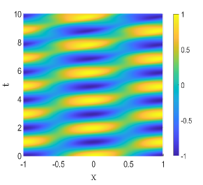
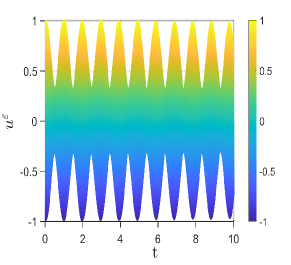
Refer to caption
Refer to caption
Refer to caption
Figure 2: The evolution of the waveform (left), the shift of profile of uεsuperscript𝑢𝜀u^{\varepsilon} (middle), the energy error in t[0,10]𝑡010t\in[0,10] (right).
Refer to caption
(a) t=0
Refer to caption
(b) t=1
Refer to caption
(c) t=5
Figure 3: The numerical solution and analytical solution at three different times.

6 Conclusions

Two regularized energy-preserving finite difference methods: the CNFD (3.4) and the SIEFD (3.5) are proposed and analyzed for the LogKGE (1.1). Error estimates were rigorously estimated by utilizing the energy method, the cut-off technique and the inverse inequality, which showed that the FDTD methods at the order O(h2+τ2ε2)𝑂superscript2superscript𝜏2superscript𝜀2O(h^{2}+\frac{\tau^{2}}{\varepsilon^{2}}) in semi-H1superscript𝐻1H^{1} norm. Besides, the error bounds were confirmed by some numerical results and the convergence order from the LogKGE to the RLogKGE is O(ε)𝑂𝜀O(\varepsilon). Based on the convergence, stability, energy conserving and computational results, we conclude that the CNFD and the SIEFD schemes are favorable for the LogKGE (1.1).

Acknowledgments

This work is supported by the National Natural Science Foundation of China (Grant No. 11971481,11901
577), the Natural Science Foundation of Hunan (Grant No.S2017JJQNJJ0764, S2020JJQNJJ1615), the Basic Research Foundation of National Numerical Wind Tunnel Project (No. NNW2018-ZT4A08). Research Fund of NUDT (Grand No. ZK17-03-27,ZK19-37), and the fund from Hunan Provincial Key Laboratory of Mathematical Modeling and Analysis in Engineering (Grand No.2018MMAEZD004).

References

References

  • [1] K. Bartkowski, P. Górka, One-dimensional Klein–Gordon equation with logarithmic nonlinearities, Journal of Physics A: Mathematical and Theoretical 41 (35) (2008) 355201.
  • [2] G. Rosen, Dilatation covariance and exact solutions in local relativistic field theories, Physical Review 183 (5) (1969) 1186.
  • [3] H. Buljan, A. Šiber, M. Soljačić, T. Schwartz, M. Segev, D. Christodoulides, Incoherent white light solitons in logarithmically saturable noninstantaneous nonlinear media, Physical Review E 68 (3) (2003) 036607.
  • [4] S. De Martino, M. Falanga, C. Godano, G. Lauro, Logarithmic Schrödinger-like equation as a model for magma transport, EPL (Europhysics Letters) 63 (3) (2003) 472.
  • [5] E. F. Hefter, Application of the nonlinear Schrödinger equation with a logarithmic inhomogeneous term to nuclear physics, Physical Review A 32 (2) (1985) 1201.
  • [6] K. Enqvist, J. McDonald, Q-balls and baryogenesis in the MSSM, Physics Letters B 425 (3-4) (1998) 309–321.
  • [7] A. Linde, Strings, textures, inflation and spectrum bending, Physics Letters B 284 (3-4) (1992) 215–222.
  • [8] W. Królikowski, D. Edmundson, O. Bang, Unified model for partially coherent solitons in logarithmically nonlinear media, Physical Review E 61 (3) (2000) 3122.
  • [9] J. J. Sakurai, Advanced quantum mechanics, Pearson Education India, 1967.
  • [10] N. Masmoudi, K. Nakanishi, From nonlinear Klein-Gordon equation to a system of coupled nonlinear Schrödinger equations, Mathematische Annalen 324 (2) (2002) 359–389.
  • [11] S. Machihara, The nonrelativistic limit of the nonlinear Klein-Gordon equation, Funkcialaj Ekvacioj Serio Internacia 44 (2) (2001) 243–252.
  • [12] E. M. Maslov, Pulsons, bubbles, and the corresponding nonlinear wave equations in n+ 1 dimensions, Physics Letters A 151 (1-2) (1990) 47–51.
  • [13] I. Bialynicki-Birula, J. Mycielski, Gaussons: solitons of the logarithmic Schrödinger equation, Physica Scripta 20 (3-4) (1979) 539.
  • [14] V. A. Koutvitsky, E. M. Maslov, Instability of coherent states of a real scalar field, Journal of mathematical physics 47 (2) (2006) 022302.
  • [15] P. Gorka, Logarithmic Klein-Gordon equation, Acta Physica Polonica B 40 (2009) 59–66.
  • [16] A. M. Wazwaz, Gaussian solitary wave solutions for nonlinear evolution equations with logarithmic nonlinearities, Nonlinear Dynamics 83 (1-2) (2016) 591–596.
  • [17] V. Makhankov, I. Bogolubsky, G. Kummer, A. Shvachka, Interaction of relativistic gaussons, Physica Scripta 23 (5A) (1981) 767.
  • [18] W. Bao, X. Dong, Analysis and comparison of numerical methods for the Klein–Gordon equation in the nonrelativistic limit regime, Numerische Mathematik 120 (2) (2012) 189–229.
  • [19] Q. Chang, G. Wang, B. Guo, Conservative scheme for a model of nonlinear dispersive waves and its solitary waves induced by boundary motion, Journal of Computational Physics 93 (2) (1991) 360–375.
  • [20] D. Duncan, Sympletic finite difference approximations of the nonlinear Klein–Gordon equation, SIAM Journal on Numerical Analysis 34 (5) (1997) 1742–1760.
  • [21] W. Bao, Y. Feng, W. Yi, Long time error analysis of finite difference time domain methods for the nonlinear Klein-Gordon equation with weak nonlinearity, arXiv preprint arXiv:1903.01133.
  • [22] Y. Luo, X. Li, C. Guo, Fourth-order compact and energy conservative scheme for solving nonlinear Klein-Gordon equation, Numerical Methods for Partial Differential Equations 33 (4) (2017) 1283–1304.
  • [23] L. Zhang, Convergence of a conservative difference scheme for a class of Klein–Gordon–Schrödinger equations in one space dimension, Applied Mathematics and Computation 163 (1) (2005) 343–355.
  • [24] W. Bao, Y. Cai, Optimal error estimates of finite difference methods for the Gross-Pitaevskii equation with angular momentum rotation, Mathematics of Computation 82 (281) (2013) 99–128.
  • [25] J. Yan, H. Zhang, X. Qian, S. Song, Regularized finite difference methods for the logarithmic Klein-Gordon equation, under review.
  • [26] B. Ji, L. Zhang, X. Zhou, Conservative compact finite difference scheme for the N-coupled nonlinear Klein–Gordon equations, Numerical Methods for Partial Differential Equations 35 (3) (2019) 1056–1079.
  • [27] W. Bao, Y. Cai, X. Zhao, A uniformly accurate multiscale time integrator pseudospectral method for the Klein–Gordon equation in the nonrelativistic limit regime, SIAM Journal on Numerical Analysis 52 (5) (2014) 2488–2511.
  • [28] W. Cao, B. Guo, Fourier collocation method for solving nonlinear Klein-Gordon equation, Journal of Computational Physics 108 (2) (1993) 296–305.
  • [29] W. Bao, Y. Feng, C. Su, Uniform error bounds of a time-splitting spectral method for the long-time dynamics of the nonlinear Klein-Gordon equation with weak nonlinearity, arXiv preprint arXiv:2001.10868.
  • [30] W. Bao, X. Dong, X. Zhao, An exponential wave integrator sine pseudospectral method for the Klein–Gordon–Zakharov system, SIAM Journal on Scientific Computing 35 (6) (2013) A2903–A2927.
  • [31] E. Faou, K. Schratz, Asymptotic preserving schemes for the Klein–Gordon equation in the non-relativistic limit regime, Numerische Mathematik 126 (3) (2014) 441–469.
  • [32] S. Jiménez, L. Vázquez, Analysis of four numerical schemes for a nonlinear Klein-Gordon equation, Applied Mathematics and Computation 35 (1) (1990) 61–94.
  • [33] P. Pascual, S. Jiménezz, L. Vázquez, Numerical simulations of a nonlinear Klein-Gordon model. Applications, in: Third Granada Lectures in Computational Physics, Springer, 1995, pp. 211–270.
  • [34] W. Bao, X. Zhao, Comparison of numerical methods for the nonlinear Klein-Gordon equation in the nonrelativistic limit regime, Journal of Computational Physics 398 (2019) 108886.
  • [35] R. P. Feynman, R. B. Leighton, M. Sands, The feynman lectures on physics; vol. i, American Journal of Physics 33 (9) (1965) 750–752.
  • [36] T. B. Benjamin, The stability of solitary waves, Proceedings of the Royal Society of London. A. Mathematical and Physical Sciences 328 (1573) (1972) 153–183.
  • [37] W. Bao, Y. Cai, Uniform error estimates of finite difference methods for the nonlinear Schrödinger equation with wave operator, SIAM Journal on Numerical Analysis 50 (2) (2012) 492–521.
  • [38] E. Celledoni, V. Grimm, R. I. McLachlan, D. McLaren, D. O Neale, B. Owren, G. Quispel, Preserving energy resp. dissipation in numerical PDEs using the Average Vector Field method, Journal of Computational Physics 231 (20) (2012) 6770–6789.
  • [39] P. Castillo, S. Gómez, Conservative local discontinuous Galerkin method for the fractional Klein-Gordon-Schrödinger system with generalized yukawa interaction, Numerical Algorithms (2019) 1–19.
  • [40] J. Cai, Y. Wang, H. Liang, Local energy-preserving and momentum-preserving algorithms for coupled nonlinear Schrödinger system, Journal of Computational Physics 239 (2013) 30–50.
  • [41] L. Brugnano, C. Zhang, D. Li, A class of energy-conserving hamiltonian boundary value methods for nonlinear Schrödinger equation with wave operator, Communications in Nonlinear Science and Numerical Simulation 60 (2018) 33–49.
  • [42] E. Celledoni, R. I. McLachlan, B. Owren, G. R. W. Quispel, Geometric properties of Kahan’s method, Journal of Physics A: Mathematical and Theoretical 46 (2) (2012) 025201.
  • [43] W. Bao, R. Carles, C. Su, Q. Tang, Error estimates of a regularized finite difference method for the logarithmic Schrödinger equation, SIAM Journal on Numerical Analysis 57 (2) (2019) 657–680.
  • [44] R. Landes, On Galerkin’s method in the existence theory of quasilinear elliptic equations, Journal of Functional Analysis 39 (2) (1980) 123–148.
  • [45] G. D. Akrivis, V. A. Dougalis, O. A. Karakashian, On fully discrete Galerkin methods of second-order temporal accuracy for the nonlinear Schrödinger equation, Numerische Mathematik 59 (1) (1991) 31–53.
  • [46] J. M. Holte, Discrete Gronwall lemma and applications, in: MAA-NCS meeting at the University of North Dakota, Vol. 24, 2009, pp. 1–7.