Understanding and Mitigating Exploding Inverses
in Invertible Neural Networks
Jens Behrmann∗1 Paul Vicol∗2,3 Kuan-Chieh Wang∗2,3 Roger Grosse2,3 Jörn-Henrik Jacobsen2,3 1University of Bremen 2University of Toronto 3Vector Institute ∗ Equal contribution
Abstract
Invertible neural networks (INNs) have been used to design generative models, implement memory-saving gradient computation, and solve inverse problems. In this work, we show that commonly-used INN architectures suffer from exploding inverses and are thus prone to becoming numerically non-invertible. Across a wide range of INN use-cases, we reveal failures including the non-applicability of the change-of-variables formula on in- and out-of-distribution (OOD) data, incorrect gradients for memory-saving backprop, and the inability to sample from normalizing flow models. We further derive bi-Lipschitz properties of atomic building blocks of common architectures. These insights into the stability of INNs then provide ways forward to remedy these failures. For tasks where local invertibility is sufficient, like memory-saving backprop, we propose a flexible and efficient regularizer. For problems where global invertibility is necessary, such as applying normalizing flows on OOD data, we show the importance of designing stable INN building blocks.
1 INTRODUCTION
Invertible neural networks (INNs) have become a standard building block in the deep learning toolkit (Papamakarios et al., 2019; Donahue and Simonyan, 2019). Invertibility is useful for training normalizing flow (NF) models with exact likelihoods (Dinh et al., 2014, 2017), increasing posterior flexibility in VAEs (Rezende and Mohamed, 2015), learning transition operators in MCMC samplers (Song et al., 2017), computing memory-efficient gradients (Gomez et al., 2017), allowing for bi-directional training (Grover et al., 2018), solving inverse problems (Ardizzone et al., 2019a) and analyzing adversarial robustness (Jacobsen et al., 2019).
![[Uncaptioned image]](/html/2006.09347/assets/img/test_intro_1g.png)
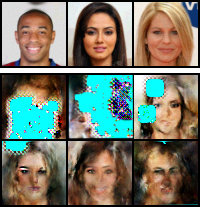
All the aforementioned applications rely on the assumption that the theoretical invertibility of INNs carries through to their numerical instantiation. In this work, we challenge this assumption by probing their inverse stability in generative and discriminative modeling settings. As a motivating example, on the left we show an image from within the dequantization distribution of a training example, and the reconstructed image from a competitive CelebA normalizing flow model (Kingma and Dhariwal, 2018). In the same vein as exploding gradients in RNNs, here the inverse mapping explodes, leading to severe reconstruction errors up to Inf/NaN values. The model exhibits similar failures both on out-of-distribution data and on samples from the model distribution (discussed in Section 4.1). Interestingly, none of these failures are immediately apparent during training. Hence, NFs can silently become non-invertible, violating the assumption underlying their main advantages—exact likelihood computation and efficient sampling (Papamakarios et al., 2019).
![[Uncaptioned image]](/html/2006.09347/assets/x1.png)
Memory-saving gradient computation (Gomez et al., 2017) is another popular application of INNs where exploding inverses can be detrimental. On the left, we show the angle between (1) gradients obtained from standard backprop and (2) memory-efficient gradients obtained using the inverse mapping to recompute activations, during training of additive- and affine-coupling INN classifiers on CIFAR-10. The affine model exhibits exploding inverses, leading to a rapidly increasing angle that becomes NaN after the dashed vertical line—making memory-efficient training infeasible—whereas the additive model is stable. This highlights the importance of understanding the influence of different INN architectures on stability. Different tasks may have different stability requirements: NFs require the model to be invertible on training and test data and, for many applications, on out-of-distribution data as well. In contrast, memory-saving gradients only require the model to be invertible on the training data, to reliably compute gradients.
As we will show in our numerical experiments, the aforementioned failures are not a rare phenomenon, but are a concern across most application areas of INNs. To provide an understanding of these failures, we study the elementary components that influence the stability of INNs: 1) bi-Lipschitz properties of INN blocks (section 3.1); 2) the effect of the training objective (section 3.3); and 3) task-specific requirements for the inverse computations (section 4 on global invertibility for change-of-variables vs. local invertibility for accurate memory-efficient gradients). Finally, putting our theoretical analysis into practice, we empirically verify solutions to overcome exploding inverses. These solutions follow two main paradigms: 1) Enforcing global stability using Lipschitz-constrained INN architectures or 2) regularization to enforce local stability. In summary, we both uncover exploding inverses as an issue across most use-cases of INNs and provide ways to mitigate this instability. Our code can be found at: http://www.github.com/asteroidhouse/INN-exploding-inverses.
2 INVERTIBLE NETWORKS
Invertible neural networks (INNs) are bijective functions with a forward mapping and an inverse mapping . This inverse can be given in closed-form (Dinh et al., 2017; Kingma and Dhariwal, 2018) or approximated numerically (Behrmann et al., 2019; Song et al., 2019). Central to our analysis of the stability of INNs is bi-Lipschitz continuity:
Definition 1 (Lipschitz and bi-Lipschitz continuity).
A function is called Lipschitz continuous if there exists a constant such that:
| (1) |
If an inverse and a constant exists such that for all
| (2) |
holds, then is called bi-Lipschitz continuous. Furthermore, or is called locally Lipschitz continuous in , if the above inequalities hold for or in the interval .
As deep-learning computations are carried out with limited precision, numerical error is always introduced in both the forward and inverse passes. Instability in either pass will aggravate this imprecision, and can make an analytically invertible network numerically non-invertible. If the singular values of the Jacobian of the inverse mapping can become arbitrarily large, we refer to this effect as an exploding inverse.
To obtain a better understanding in the context of INNs, we first define coupling blocks and then study numerical error and instability in a toy setting. Let denote disjoint index sets of to partition vectors . For example, they denote a partition of feature channels in a convolutional architecture. Additive coupling blocks (Dinh et al., 2014) are defined as:
| (3) | ||||
and affine coupling blocks (Dinh et al., 2017) as:
| (4) | ||||
where are Lipschitz continuous and denotes elementwise multiplication. Hence, coupling blocks differ only in their scaling 111Affine blocks scale the input with an elementwise function that has to be non-zero everywhere—common choices are sigmoid or ..
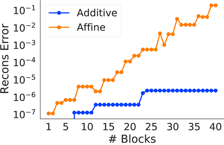
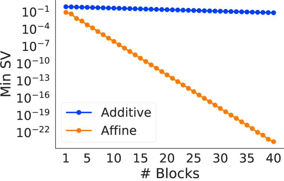
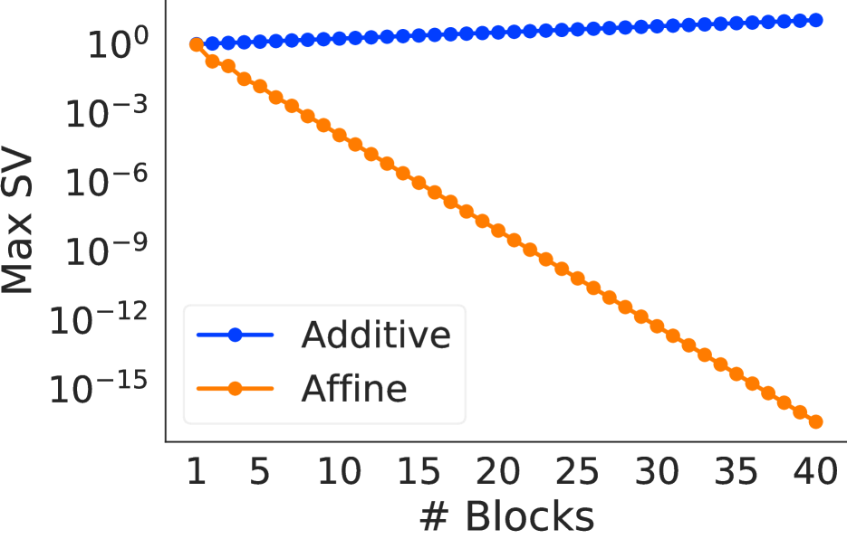
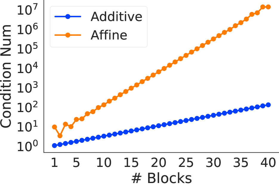
To understand how numerical error occurs in coupling blocks, consider the following example: consider and the trivial partition and . Further, let and . Floating-point operations introduce rounding errors when numbers from different scales are summed up. Figure 1 visualizes the reconstruction error introduced at various depth for the given . In particular, the additive coupling INN has small numerical errors when reconstructing due to rounding errors in the summation. The affine blocks, however, show an exploding inverse effect since the singular values of the forward mapping tend to zero as depth increases. Thus, while being analytically invertible, the numerical errors and instability renders the network numerically non-invertible even in this simple example.
To formalize the connection of numerical errors and Lipschitz constants, consider as the analytical exact forward computation and as the floating-point inexact computation with error . In order to bound the error in the reconstruction due to the imprecision in the forward mapping, let . Now consider:
where is used to bound the influence of the numerical error introduced in the forward mapping. Additionally, similarly to the forward mapping, the inverse mapping adds numerical imprecision. Thus, we introduce . Hence, we obtain the bound:
While obtaining quantitative values for and for a model as complex as deep INNs is hard, the above formalization still provides insights into the role of the inverse stability when reconstructing inputs. In sum, INNs are designed to be analytically invertible, but numerical errors are always present. How much these errors are magnified is bounded by their Lipschitz continuity (stability).
3 STABILITY OF INVERTIBLE NEURAL NETWORKS
We first discuss bi-Lipschitz properties of common INN building blocks, and how certain architectures suffer from exploding inverses in Section 3.1. Then we explore how to stabilize INNs globally (Section 3.2) and locally (Section 3.3).
3.1 Lipschitz Properties of INN Blocks
Research on INNs has produced a large variety of architectural building blocks. Here, we build on the work of Behrmann et al. (2019), that proved bi-Lipschitz bounds for invertible ResNets. In particular, we derive Lipschitz bounds of coupling-based INNs and provide an overview of the stability of other common building blocks. Most importantly for our subsequent discussion are the qualitative insights we can draw from this analysis. Hence, we summarize these results in Theorem 2 and provide the quantitative Lipschitz bounds as lemmas in Appendix B.
We start with our main result on coupling blocks, which are the most commonly used INN architectures. While they only differ in the scaling, this difference strongly influences stability:
Theorem 2 (Stability of additive and affine blocks).
Consider additive and affine blocks as in Eq. 3 and Eq. 4 and assume the same function . Further, let Lipschitz continuous, continuously differentiable and non-constant functions. Then the following differences w.r.t. bi-Lipschitz continuity hold:
-
(i)
Affine blocks have strictly larger (local) bi-Lipschitz bounds than additive blocks.
- (ii)
The proof is given in Appendix B.1, together with upper bounds in Lemmas 5 and 6. Note that an upper bound on provides a lower bound on and vice versa. These differences offer two main insights. First, affine blocks can have arbitrarily large singular values in the inverse Jacobian, i.e. an exploding inverse. Thus, they are more likely to become numerically non-invertible than additive blocks. Second, controlling stability in each architecture requires fundamentally different approaches since additive blocks have global bounds, while affine blocks are not globally bi-Lipschitz.
In addition to the Lipschitz bounds of coupling layers, we provide an overview of known Lipschitz bounds of other common INN building blocks in Table 3 (Appendix A). Besides coupling-based approaches we cover free-form approaches like Neural ODEs (Chen et al., 2018) and i-ResNets (Behrmann et al., 2019). Note that the bounds provide the worst-case stability and are primarily meant to serve as a guideline for the design of invertible blocks.
3.2 Controlling Global Stability of INNs
As we showed in the previous section, each INN building block has its own stability properties (see Table 3 for an overview). The bi-Lipschitz bounds of additive coupling blocks can be controlled using a similar strategy to i-ResNets. Via spectral normalization (Miyato et al., 2018), it is possible to control the Lipschitz-constant of in Eq. 3, which guarantees stability via the bounds from Lemma 5. On the other hand, spectral normalization does not provide guarantees for affine blocks, as they are not globally bi-Lipschitz over due to dependence on the range of the inputs (see Theorem 2).
Modified Affine Scaling.
A natural way to increase stability of affine blocks is to consider different elementwise scaling functions , see Ardizzone et al. (2019b) for an example of such a modification. In particular, avoiding scaling by small values strongly influences the inverse Lipschitz bound (see Lemma 6, Appendix B). Thus, a modification guided by Lemma 6 would be to adapt the sigmoid scaling to output values in a restricted range such as rather than the standard range . As we show in our experiments (Sections 4.1.1 & 4.1.2), this indeed improves stability. However, it may still suffer from exploding inverses as there is no global Lipschitz bound (see Theorem 2).
3.3 Controlling Local Stability of INNs
While the previous section aimed at controlling global stability, in this section we discuss how penalty functions and the training objective itself stabilize INNs locally, i.e. around inputs .
3.3.1 Bi-Directional Finite Differences Regularization
Penalty terms on the Jacobian can be used to enforce local stability (Sokolić et al., 2017; Hoffman et al., 2019). Their connection to Lipschitz bounds can be understood using the identity from Federer (1969, Thm. 3.1.6): if is Lipschitz continuous and differentiable, then we have:
| (5) |
where is the Jacobian matrix of at and denotes its spectral norm. To approximate the RHS of Eq. 3.3.1 from below, we obtain as with , which uniformly samples from the unit sphere (Muller, 1959). For given and , the term can be added to the loss function as a regularizer. However, training with such a penalty term requires double-backpropagtion (Drucker and Le Cun, 1992; Etmann, 2019), which makes recomputing the pre-activations during backprop via the inverse (Gomez et al., 2017) (memory-saving gradients) difficult. Thus, in addition to randomization, we introduce a second approximation using finite differences as:
| (6) |
with a step-size . The approximation error can be estimated via Taylor expansion and has to be traded off with catastrophic cancellation due to subtracting near-identical float values (An et al., 2011). Since we aim at having both stable forward and inverse mappings, we employ this penalty on both directions and , and call it bi-directional finite differences regularization (abbreviated FD). Details about this architecture agnostic regularizer and its computational overhead are provided in Appendix G.
Glow
{annotate}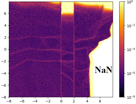 1
\draw[thick,dashed,green] (-1.18,-0.82) rectangle (0.66,0.98);
Glow w/ Modified Scaling
{annotate}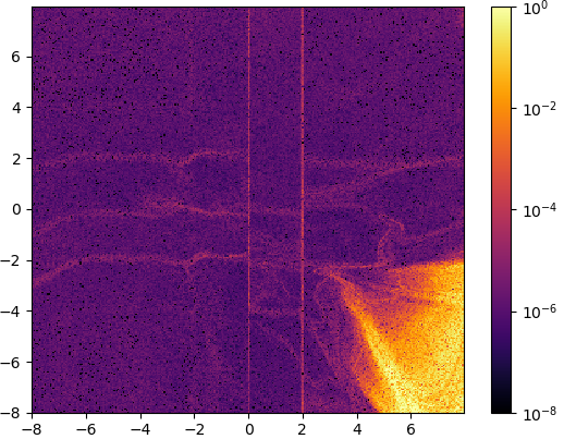 1
\draw[thick,dashed,green] (-1.18,-0.82) rectangle (0.66,0.98);
Residual Flow
{annotate}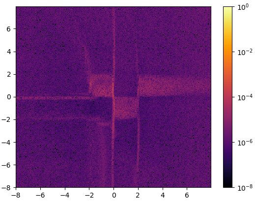 1
\draw[thick,dashed,green] (-1.18,-0.82) rectangle (0.66,0.98);
1 \draw[thick,dashed,green] (-0.80,-0.86) rectangle (1.04,0.94);
3.3.2 Influence of the Normalizing Flow Loss on Stability
In addition to the INN architecture and local regularization such as bi-directional FD introduced in Section 3.3.1, the training objective itself can impact local stability. Here, we examine the stabilization effect of the commonly used normalizing flow (NF) objective (Papamakarios et al., 2019). Consider a parametrized diffeomorphism and a base distribution . By a change-of-variables, we have for all
| (7) |
where denotes the Jacobian of at . The log-determinant in Eq. 7 can be expressed as:
| (8) |
where denotes the -th singular value of . Thus, minimizing the negative log-likelihood as involves maximizing the sum of the log singular values (Eq. 8). Due to the slope of the logarithmic function , very small singular values are avoided more strongly than large singular values are favored. Thus, the inverse of is encouraged to be more stable than the forward mapping. Furthermore when using as the base distribution, we minimize:
which bounds the -norm of the outputs of . Due to this effect, large singular values are avoided and the mapping is further locally stabilized.
Thus, the two terms of the normalizing flow objective have complementary effects on stability: the log-determinant increases all singular values, but has a stronger effect on small singular values than on large ones, improving inverse stability, while the base term encourages the output of the function to have small magnitude, improving forward stability. If additional stability is required, bounding the -norm of intermediate activations would further avoid fluctuations, where a subflow exhibits high magnitude that is cancelled out by the subsequent subflow. The effect of the NF objective, however, acts only on the training data and is thus not able to globally stabilize INNs, as we show in our experiments (Section 4.1).
4 EXPERIMENTS
First, we show that exploding inverses are a concern across most application areas of INNs. Second, we aim to provide ways to mitigate instability. For this we conduct experiments on two tasks: generative modeling with normalizing flows (Section 4.1) and memory-efficient gradient computation for supervised learning (Section 4.2). Due to the growing body of INN architectures we had to restrict our experimental study to a subset of INNs: additive/ affine coupling blocks (Dinh et al., 2014, 2017) and Residual Flows (Chen et al., 2019). This particular choice was guided by the simplicity of coupling blocks and by the close link of Residual Flows to stability.
4.1 Non-Invertibility in Normalizing Flows
Here we show that INNs can become numerically non-invertible even when trained with the normalizing flow (NF) loss (despite encouraging local stability, see Section 3.3.2). We study this behavior on out-of-distribution data and identify the exploding inverse effect in the data and model distribution.
4.1.1 Instability on Out-of-Distribution Data
|
|
||||||||||||||||||||||||||||||||||||||||||||||||||||||||||||||
Because NFs allow for efficient likelihood computation, they have been used in several likelihood-based approaches for out-of-distribution (OOD) detection (Nalisnick et al., 2019; Fetaya et al., 2020). Here we show, however, that certain classes of flows can be numerically non-invertible on OOD data, implying that the likelihoods computed on such data are not meaningful because the change-of-variables formula no longer applies.
2D Checkerboard.
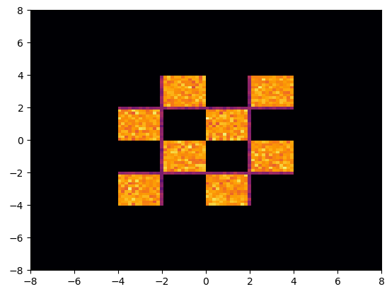
First we consider a 2D checkerboard distribution (see samples in Figure 3 and further details in Appendix C). Despite being ill-posed due to the discontinuous density (jumps at the edges of the checkerboard), it is often used as a benchmark for NFs (Chen et al., 2019; Grathwohl et al., 2019). The discontinuity of the dataset is manifested in two main ways in Figure 2: 1) at these jumps, the model becomes unstable, which leads to larger reconstruction errors (see slightly expressed grid-like pattern), 2) affine models can become non-invertible outside the data domain. Figure 2 further shows reconstruction errors from a modified affine model—which is more stable, but still suffers from exploding inverses in OOD areas—and a Residual Flow (Chen et al., 2019), which has low reconstruction error globally, consistent with our stability analysis.
| Additive | Affine | Mod. Affine | |
|---|---|---|---|
| Data BPD (Train) | 3.29 | 3.27 | 3.25 |
| Data BPD (Test) | 3.55 | 3.51 | 3.5 |
| Reliable Sample BPD | ✓ | ✗ | ✓ |
| No Visible Sample Recon Err. | ✓ | ✗ | ✓ |
CIFAR-10 OOD.
Next, we evaluated CIFAR-10 pre-trained Glow and Residual Flow models on a set of OOD datasets from Hendrycks and Gimpel (2016); Liang et al. (2017); Nalisnick et al. (2019). 222For Glow and Residual Flows, we used the pre-trained models from https://github.com/y0ast/Glow-PyTorch and https://github.com/rtqichen/residual-flows, respectively. Figure 4 shows qualitative reconstruction errors for Glow on three OOD datasets, as well as the numerical reconstruction errors for Glow and ResFlow models on all OOD datasets. While the Residual Flow was always stably invertible, Glow was non-invertible on all datasets except SVHN. This indicates that OOD detection methods based on Glow likelihoods may be unreliable. In Appendix D, we provide additional details, as well as a comparison of the stability of additive and affine coupling models on OOD data during training.
4.1.2 Instability in the Data Distribution and further Failures
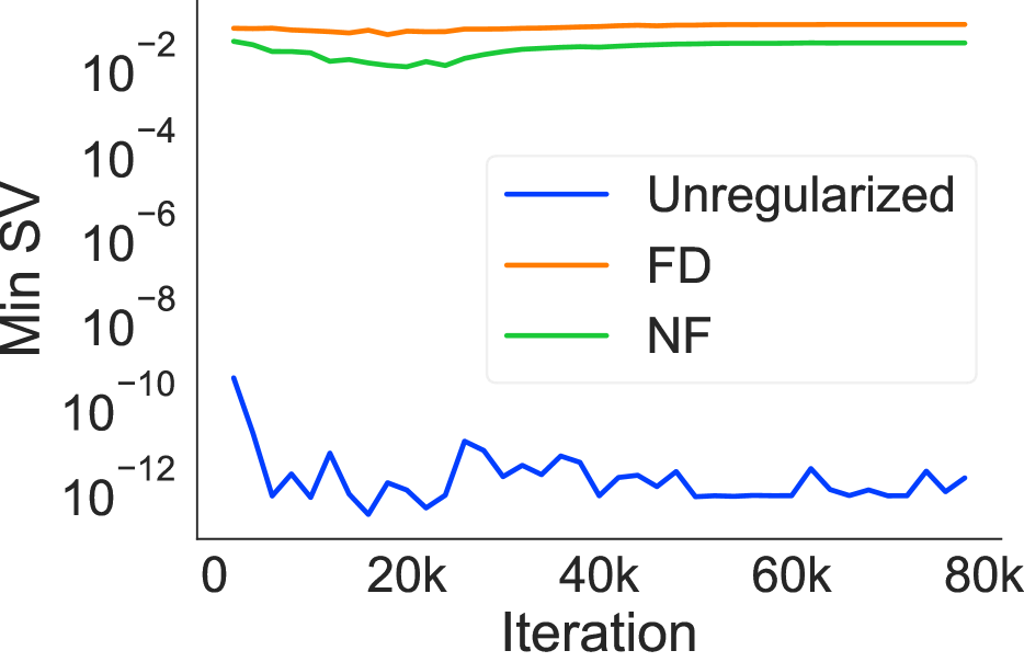
| Unregularized Regularized |
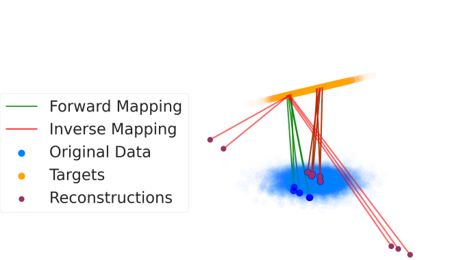
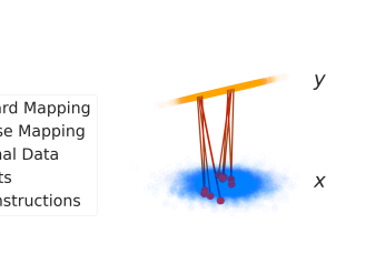
|
In this section, we further identify failures within the model and data distributions. In particular, we study the stability of the inverse on the model distribution by sampling from the base distribution (rather than obtaining via a forward pass on some data). For this, we trained both additive/affine models on CIFAR-10, and an affine model on CelebA64 (see details in Appendix D). We report quantitative results during training on CIFAR-10 in Table 1. The affine model was unstable w.r.t. model samples. Furthermore in Figure 6, we show samples from the affine CelebA64 model, which has NaN values in multiple samples.
Non-Invertible Inputs within the Dequantization Region.
We can further expose non-invertibility even in the data distribution. By optimizing within the dequantization distribution of a datapoint we are able to find regions that are poorly reconstructed by the model. Note that the inputs found this way are valid samples from the training data distribution. See Appendix E for details.
Instability beyond the NF loss.
In Appendix H we provide results on bi-directional training with INNs in the Flow-GAN setting (Grover et al., 2018). While additive models did not show instabilities thus far, they exhibit exploding inverses when trained solely adversarially. Lastly, this exploration demonstrates how our analysis can be leveraged to choose appropriate tools for stabilizing INNs, and in this case improve model samples while retaining competitive bits-per-dimension (BPDs).
4.2 Supervised Learning with Memory Efficient Gradients
For supervised learning, INNs enable memory-efficient training by re-computing intermediate activations in the backward pass, rather than storing them in memory during the forward pass (Gomez et al., 2017). This enables efficient large-scale generative modeling (Donahue and Simonyan, 2019) and high-resolution medical image analysis (Etmann et al., 2020). Re-computing the activations during the backward pass, however, relies on the inverse being numerically precise locally around the training data. This is a weaker requirement than the global stability we desire for NFs such that they can be applied to OOD data. However, in this section we show that even this weaker requirement can be violated, and how to mitigate these failures by local regularization as discussed in Section 3.3.
Toy 2D Regression.
In contrast to NFs, where the likelihood objective encourages local stability, there is no default mechanism to avoid unstable inverses in supervised learning (e.g., classification or regression). As an example, consider a simple 2D regression problem visualized in Figure 7. Here, the targets lie almost on a 1D subspace, which requires the learned mapping to contract from 2D to 1D. Even in such a simple task, a Glow regression model becomes non-invertible, as shown by the misplaced reconstructions for the unregularized model. Additional details are provided in Appendix F. This illustrates the importance of adding regularization terms to supervised objectives to maintain invertibility, as we do next for memory-efficient training on CIFAR-10.
CIFAR-10 Classification.
Here we show that INN classifiers on CIFAR-10 can become non-invertible—making it impossible to compute accurate memory-saving gradients—and that local regularization by adding either the finite differences (FD) penalty or the normalizing flow (NF) objective with a small coefficient stabilizes these models, enabling memory-efficient training. We focused on additive and affine models with architectures similar to Glow (Kingma and Dhariwal, 2018), with either convolutions or shuffle permutations and ActNorm between building blocks. We used only coupling approaches, because i-ResNets (Behrmann et al., 2019) are not suited for memory-efficient gradients due to their use of an expensive iterative inverse. Experimental details and extended results are provided in Appendix G.
| Model | Regularizer | Inv? | Test Acc | Recons. Err. | Cond. Num. | Min SV | Max SV |
|---|---|---|---|---|---|---|---|
| Additive Conv | None | ✓ | 89.73 | 4.3e-2 | 7.2e+4 | 6.1e-2 | 4.4e+3 |
| FD | ✓ | 89.71 | 1.1e-3 | 3.0e+2 | 8.7e-2 | 2.6e+1 | |
| NF | ✓ | 89.52 | 9.9e-4 | 1.7e+3 | 3.9e-2 | 6.6e+1 | |
| Affine Conv | None | ✗ | 89.07 | Inf | 8.6e14 | 1.9e-12 | 1.7e+3 |
| FD | ✓ | 89.47 | 9.6e-4 | 1.6e+2 | 9.6e-2 | 1.5e+1 | |
| NF | ✓ | 89.71 | 1.3e-3 | 2.2e+3 | 3.5e-2 | 7.7e+1 |
In Table 2, we compare the performance and stability properties of unregularized additive and affine models, as well as regularized versions using either FD or NF penalties (Appendix G shows the effects of different regularization strengths). Note that we do not aim to achieve SOTA accuracy, and these accuracies match those reported for a similar Glow classifier by Behrmann et al. (2019). In particular, we observe how affine models suffer from exploding inverses and are thus not suited for computing memory-efficient gradients. Both the NF and FD regularizers mitigate the instability, yielding similar test accuracies to the unregularized model, while maintaining small reconstruction errors and condition numbers.333Note that the training with FD was performed memory-efficiently, while the None and NF settings were trained using standard backprop. In Appendix G, we show that regularization keeps the angle between the true gradient and memory-saving gradient small throughout training. The computational overhead of the FD regularizer is only 1.26 that of unregularized training (Table 11 in App. G). We also experimented with applying the FD regularizer only to the inverse mapping, and while this can also stabilize the inverse and achieve similar accuracies, we found bi-directional FD to be more reliable across architectures. Applying regularization once every 10 iterations, bi-FD is only 1.06 slower than inverse-FD. As the FD regularizer is architecture agnostic and conceptually simple, we envision a wide-spread use for memory-efficient training.
5 RELATED WORK
Invertibility and Stability of Deep Networks.
The inversion from activations in standard neural networks to inputs has been studied via optimization in input space (Mahendran and Vedaldi, 2014) or by linking invertibility and inverse stability for ReLU-networks (Behrmann et al., 2018). However, few works have studied the stability of INNs: Gomez et al. (2017) examined the numerical errors in the gradient computation when using memory-efficient backprop. Similarly to our empirical analysis, Jacobsen et al. (2018) computed the SVD of the Jacobian of an i-RevNet and found it to be ill-conditioned. Furthermore, i-ResNets (Behrmann et al., 2019) yield bi-Lipschitz bounds by design. Lastly, Chang et al. (2018) studied the stability of reversible INN dynamics in a continuous framework. In contrast, the stability of neural networks has been of major interest due to the problem of exploding/vanishing gradients as well as for training Wasserstein GANs (Arjovsky et al., 2017). Furthermore, adversarial examples (Szegedy et al., 2013) are strongly tied to stability and inspired our invertibility attack (Section 4.1.2).
Improving Stability of Invertible Networks.
Instability in INNs has been noticed in other works, yet without a detailed treatment. For example, Putzky and Welling (2019) proposed to employ orthogonal convolutions to obtain accurate memory-efficient gradients and Etmann et al. (2020) used weight normalization for stabilization. Our finite differences regularizer, on the other hand, is architecture agnostic and could be used in the settings above. Furthermore, Ardizzone et al. (2019b) considered modified scaling in affine models to improve their stability. Neural ODEs (Chen et al., 2018) are another way to design INNs, and research their stability. Finlay et al. (2020); Yan et al. (2020); Massaroli et al. (2020) provide further insights into designing principled and stable INNs.
Fixed-Point Arithmetic in INNs.
Maclaurin et al. (2015); MacKay et al. (2018) implement invertible computations using fixed-point numbers, with custom schemes to store information that is lost when bits are shifted, enabling exact invertibility at the cost of memory usage. As Gomez et al. (2017) point out, this allows exact numerical inversion when using additive coupling independent of stability. However, our stability analysis aims for a broadly applicable methodology beyond the special case of additive coupling.
Invertible Building Blocks.
Besides the invertible building blocks listed in Table 3 (Appendix A), several other approaches like in Karami et al. (2019) have been proposed. Most prominently, autogressive models like IAF (Kingma et al., 2016), MAF (Papamakarios et al., 2017) or NAF (Huang et al., 2018) provide invertible models that are not studied in our analysis. Furthermore, several newer coupling layers that require numerical inversion have been introduced by Ho et al. (2019); Jaini et al. (2019); Durkan et al. (2019). In addition to the coupling-based approaches, multiple approaches (Chen et al., 2018; Behrmann et al., 2019; Chen et al., 2019; Grathwohl et al., 2019; Song et al., 2019) use numerical inversion schemes, where the interplay of numerical error due to stability and error due to the approximation of the inverse adds another dimension to the study of invertibility.
Stability-Expressivity Tradeoff.
While Lipschitz constrained INNs like i-ResNets (Behrmann et al., 2019) allow to overcome many failures we observed with affine coupling blocks (Dinh et al., 2017), this constrains the flexibility of INNs. Hence, there is a tradeoff between stability and expressivity as studied in Jaini et al. (2020); Cornish et al. (2020). While numerical invertibility is necessary for a safe usage of INNs, mixtures of Lipschitz constrained INNs could be used for improved flexibility as suggested in Cornish et al. (2020).
6 CONCLUSION
Invertible Neural Networks (INNs) are an increasingly popular component of the modern deep learning toolkit. However, if analytical invertibility does not carry through to the numerical computation, their underlying assumptions break. When applying INNs, it is important to consider how the inverse is used. If local stability is sufficient, like for memory-efficient gradients, our finite difference penalty is sufficient as an architecture agnostic stabilizer. For global stability requirements e.g. when using INNs as normalizing flows, the focus should be on architectures that enable stable mappings like Residual Flows (Chen et al., 2019). Altogether we have shown that studying stability properties of both forward and inverse is a key step towards a complete understanding of INNs.
Acknowledgements
Resources used in preparing this research were provided, in part, by the Province of Ontario, the Government of Canada through CIFAR, and companies sponsoring the Vector Institute www.vectorinstitute.ai/#partners. Jens Behrmann acknowledges the support by the Deutsche Forschungsgemeinschaft (DFG) within the framework of GRK 2224/1 “: Parameter Identification – Analysis, Algorithms, Applications”. Paul Vicol was supported by a JP Morgan AI Fellowship. We also would like to thank Joost van Amersfoort for insightful discussions, and members on the Vector’s Ops team (George Mihaiescu, Relu Patrascu, and Xin Li) for their computation/infrastructure support.
References
- An et al. (2011) Heng-Bin An, Ju Wen, and Tao Feng. On finite difference approximation of a matrix-vector product in the Jacobian-free Newton–Krylov method. Journal of Computational and Applied Mathematics, 236(6):1399 – 1409, 2011.
- Ardizzone et al. (2019a) Lynton Ardizzone, Jakob Kruse, Sebastian Wirkert, Daniel Rahner, Eric W Pellegrini, Ralf S Klessen, Lena Maier-Hein, Carsten Rother, and Ullrich Köthe. Analyzing inverse problems with invertible neural networks. In International Conference on Learning Representations, 2019a.
- Ardizzone et al. (2019b) Lynton Ardizzone, Carsten Lüth, Jakob Kruse, Carsten Rother, and Ullrich Köthe. Guided image generation with conditional invertible neural networks. arXiv preprint arXiv:1907.02392, 2019b.
- Arjovsky et al. (2017) Martin Arjovsky, Soumith Chintala, and Léon Bottou. Wasserstein generative adversarial networks. In International Conference on Machine Learning, 2017.
- Ascher (2008) Uri M. Ascher. Numerical methods for evolutionary differential equations. Computational Science and Engineering. Society for Industrial and Applied Mathematics, 2008.
- Behrmann et al. (2018) Jens Behrmann, Sören Dittmer, Pascal Fernsel, and Peter Maaß. Analysis of invariance and robustness via invertibility of ReLU-networks. arXiv preprint arXiv:1806.09730, 2018.
- Behrmann et al. (2019) Jens Behrmann, Will Grathwohl, Ricky T. Q. Chen, David Duvenaud, and Jörn-Henrik Jacobsen. Invertible residual networks. In International Conference on Machine Learning, 2019.
- Chang et al. (2018) Bo Chang, Lili Meng, Eldad Haber, Lars Ruthotto, David Begert, and Elliot Holtham. Reversible architectures for arbitrarily deep residual neural networks. In AAAI Conference on Artificial Intelligence, 2018.
- Chen et al. (2018) Ricky T. Q. Chen, Yulia Rubanova, Jesse Bettencourt, and David Duvenaud. Neural ordinary differential equations. In Advances in Neural Information Processing Systems, 2018.
- Chen et al. (2019) Ricky T. Q. Chen, Jens Behrmann, David Duvenaud, and Jörn-Henrik Jacobsen. Residual flows for invertible generative modeling. In Advances in Neural Information Processing Systems, 2019.
- Cimpoi et al. (2014) Mircea Cimpoi, Subhransu Maji, Iasonas Kokkinos, Sammy Mohamed, and Andrea Vedaldi. Describing textures in the wild. In Conference on Computer Vision and Pattern Recognition, 2014.
- Cornish et al. (2020) Rob Cornish, Anthony Caterini, George Deligiannidis, and Arnaud Doucet. Relaxing bijectivity constraints with continuously indexed normalising flows. In International Conference on Machine Learning, 2020.
- Dinh et al. (2014) Laurent Dinh, David Krueger, and Yoshua Bengio. NICE: Non-linear independent components estimation. arXiv preprint arXiv:1410.8516, 2014.
- Dinh et al. (2017) Laurent Dinh, Jascha Sohl-Dickstein, and Samy Bengio. Density estimation using real NVP. In International Conference on Learning Representations, 2017.
- Donahue and Simonyan (2019) Jeff Donahue and Karen Simonyan. Large scale adversarial representation learning. In Advances in Neural Information Processing Systems, 2019.
- Drucker and Le Cun (1992) Harris Drucker and Yann Le Cun. Improving generalization performance using double backpropagation. IEEE Transactions on Neural Networks, 3(6):991–997, 1992.
- Durkan et al. (2019) Conor Durkan, Artur Bekasov, Ian Murray, and George Papamakarios. Neural spline flows. In Advances in Neural Information Processing Systems, 2019.
- Etmann (2019) Christian Etmann. A closer look at double backpropagation. arXiv preprint arXiv:1906.06637, 2019.
- Etmann et al. (2020) Christian Etmann, Rihuan Ke, and Carola-Bibiane Schönlieb. iUNets: Fully invertible U-Nets with learnable up- and downsampling. arXiv preprint arXiv:2005.05220, 2020.
- Federer (1969) Herbert Federer. Geometric Measure Theory. Grundlehren der Mathematischen Wissenschaften. Springer, 1969.
- Fetaya et al. (2020) Ethan Fetaya, Jörn-Henrik Jacobsen, Will Grathwohl, and Richard Zemel. Understanding the limitations of conditional generative models. In International Conference on Learning Representations, 2020.
- Finlay et al. (2020) Chris Finlay, Jörn-Henrik Jacobsen, Levon Nurbekyan, and Adam M Oberman. How to train your neural ODE: The world of Jacobian and kinetic regularization. arXiv preprint arXiv:2002.02798, 2020.
- Gomez et al. (2017) Aidan N Gomez, Mengye Ren, Raquel Urtasun, and Roger B Grosse. The reversible residual network: Backpropagation without storing activations. In Advances in Neural Information Processing Systems, pages 2214–2224, 2017.
- Grathwohl et al. (2019) Will Grathwohl, Ricky T. Q. Chen, Jesse Bettencourt, Ilya Sutskever, and David Duvenaud. FFJORD: Free-form continuous dynamics for scalable reversible generative models. In International Conference on Learning Representations, 2019.
- Grover et al. (2018) Aditya Grover, Manik Dhar, and Stefano Ermon. Flow-GAN: Combining maximum likelihood and adversarial learning in generative models. In Thirty-Second AAAI Conference on Artificial Intelligence, 2018.
- Gulrajani et al. (2017) Ishaan Gulrajani, Faruk Ahmed, Martin Arjovsky, Vincent Dumoulin, and Aaron C Courville. Improved training of Wasserstein GANs. In Advances in Neural Information Processing Systems, pages 5767–5777, 2017.
- Hendrycks and Gimpel (2016) Dan Hendrycks and Kevin Gimpel. A baseline for detecting misclassified and out-of-distribution examples in neural networks. arXiv preprint arXiv:1610.02136, 2016.
- Ho et al. (2019) Jonathan Ho, Xi Chen, Aravind Srinivas, Yan Duan, and Pieter Abbeel. Flow++: Improving flow-based generative models with variational dequantization and architecture design. In International Conference on Machine Learning, 2019.
- Hoffman et al. (2019) Judy Hoffman, Daniel A. Roberts, and Sho Yaida. Robust learning with Jacobian regularization. arXiv preprint arXiv:1908.02729, 2019.
- Huang et al. (2018) Chin-Wei Huang, David Krueger, Alexandre Lacoste, and Aaron Courville. Neural autoregressive flows. In International Conference on Machine Learning, 2018.
- Jacobsen et al. (2018) Jörn-Henrik Jacobsen, Arnold Smeulders, and Edouard Oyallon. i-RevNet: Deep invertible networks. In International Conference on Learning Representations, 2018.
- Jacobsen et al. (2019) Jörn-Henrik Jacobsen, Jens Behrmann, Richard Zemel, and Matthias Bethge. Excessive invariance causes adversarial vulnerability. In International Conference on Learning Representations, 2019.
- Jaini et al. (2019) Priyank Jaini, Kira A. Selby, and Yaoliang Yu. Sum-of-squares polynomial flow. In International Conference on Machine Learning, 2019.
- Jaini et al. (2020) Priyank Jaini, Ivan Kobyzev, Yaoliang Yu, and Marcus Brubaker. Tails of Lipschitz triangular flows. In International Conference on Machine Learning, 2020.
- Karami et al. (2019) Mahdi Karami, Dale Schuurmans, Jascha Sohl-Dickstein, Laurent Dinh, and Daniel Duckworth. Invertible convolutional flow. In Advances in Neural Information Processing Systems. 2019.
- Kingma and Dhariwal (2018) Durk P Kingma and Prafulla Dhariwal. Glow: Generative flow with invertible 1x1 convolutions. In Advances in Neural Information Processing Systems, pages 10215–10224, 2018.
- Kingma et al. (2016) Durk P Kingma, Tim Salimans, Rafal Jozefowicz, Xi Chen, Ilya Sutskever, and Max Welling. Improved variational inference with inverse autoregressive flow. In Advances in Neural Information Processing Systems, pages 4743–4751, 2016.
- Liang et al. (2017) Shiyu Liang, Yixuan Li, and Rayadurgam Srikant. Enhancing the reliability of out-of-distribution image detection in neural networks. arXiv preprint arXiv:1706.02690, 2017.
- MacKay et al. (2018) Matthew MacKay, Paul Vicol, Jimmy Ba, and Roger B Grosse. Reversible recurrent neural networks. In Advances in Neural Information Processing Systems, pages 9029–9040, 2018.
- Maclaurin et al. (2015) Dougal Maclaurin, David Duvenaud, and Ryan Adams. Gradient-based hyperparameter optimization through reversible learning. In International Conference on Machine Learning, pages 2113–2122, 2015.
- Madry et al. (2018) Aleksander Madry, Aleksandar Makelov, Ludwig Schmidt, Dimitris Tsipras, and Adrian Vladu. Towards deep learning models resistant to adversarial attacks. In International Conference on Learning Representations, 2018.
- Mahendran and Vedaldi (2014) Aravindh Mahendran and Andrea Vedaldi. Understanding deep image representations by inverting them. In Conference on Computer Vision and Pattern Recognition, 2014.
- Massaroli et al. (2020) Stefano Massaroli, Michael Poli, Michelangelo Bin, Jinkyoo Park, Atsushi Yamashita, and Hajime Asama. Stable neural flows. arXiv preprint arXiv:2003.08063, 2020.
- Miyato et al. (2018) Takeru Miyato, Toshiki Kataoka, Masanori Koyama, and Yuichi Yoshida. Spectral normalization for generative adversarial networks. In International Conference on Learning Representations, 2018.
- Muller (1959) Mervin E. Muller. A note on a method for generating points uniformly on n-dimensional spheres. Commun. ACM, 2(4):19–20, 1959.
- Nalisnick et al. (2019) Eric Nalisnick, Akihiro Matsukawa, Yee Whye Teh, Dilan Gorur, and Balaji Lakshminarayanan. Do deep generative models know what they don’t know? In International Conference on Learning Representations, 2019.
- Netzer et al. (2011) Yuval Netzer, Tao Wang, Adam Coates, Alessandro Bissacco, Bo Wu, and Andrew Y Ng. Reading digits in natural images with unsupervised feature learning. In NIPS Workshop on Deep Learning and Unsupervised Feature Learning, 2011.
- Papamakarios et al. (2017) George Papamakarios, Theo Pavlakou, and Iain Murray. Masked autoregressive flow for density estimation. In Advances in Neural Information Processing Systems, pages 2338–2347, 2017.
- Papamakarios et al. (2019) George Papamakarios, Eric Nalisnick, Danilo Jimenez Rezende, Shakir Mohamed, and Balaji Lakshminarayanan. Normalizing flows for probabilistic modeling and inference. arXiv preprint arXiv:1912.02762, 2019.
- Paszke et al. (2019) Adam Paszke, Sam Gross, Francisco Massa, Adam Lerer, James Bradbury, Gregory Chanan, Trevor Killeen, Zeming Lin, Natalia Gimelshein, Luca Antiga, et al. PyTorch: An imperative style, high-performance deep learning library. In Advances in Neural Information Processing Systems, pages 8024–8035, 2019.
- Putzky and Welling (2019) Patrick Putzky and Max Welling. Invert to learn to invert. In Advances in Neural Information Processing Systems, 2019.
- Rezende and Mohamed (2015) Danilo Rezende and Shakir Mohamed. Variational inference with normalizing flows. In International Conference on Machine Learning, pages 1530–1538, 2015.
- Sokolić et al. (2017) Jure Sokolić, Raja Giryes, Guillermo Sapiro, and Miguel R. D. Rodrigues. Robust large margin deep neural networks. IEEE Transactions on Signal Processing, 65(16):4265–4280, 2017.
- Song et al. (2017) Jiaming Song, Shengjia Zhao, and Stefano Ermon. A-NICE-MC: Adversarial training for MCMC. In Advances in Neural Information Processing Systems, pages 5140–5150, 2017.
- Song et al. (2019) Yang Song, Chenlin Meng, and Stefano Ermon. MintNet: Building invertible neural networks with masked convolutions. In Advances in Neural Information Processing Systems, 2019.
- Szegedy et al. (2013) Christian Szegedy, Wojciech Zaremba, Ilya Sutskever, Joan Bruna, Dumitru Erhan, Ian Goodfellow, and Rob Fergus. Intriguing properties of neural networks. arXiv preprint arXiv:1312.6199, 2013.
- Yan et al. (2020) Hanshu Yan, Jiawei Du, Vincent Tan, and Jiashi Feng. On robustness of neural ordinary differential equations. In International Conference on Learning Representations, 2020.
- Zhang et al. (2019) Guodong Zhang, Chaoqi Wang, Bowen Xu, and Roger Grosse. Three mechanisms of weight decay regularization. In International Conference on Learning Representations, 2019.
- Zhou et al. (2017) Bolei Zhou, Agata Lapedriza, Aditya Khosla, Aude Oliva, and Antonio Torralba. Places: A 10 million image database for scene recognition. IEEE Transactions on Pattern Analysis and Machine Intelligence, 2017.
Understanding and Mitigating Exploding Inverses
in Invertible Neural Networks
SUPPLEMENTARY MATERIAL
-
•
In Section A we provide a table of Lipschitz bounds for various INN building blocks.
-
•
In Section B we provide statements on Lipschitz bounds and their corresponding proofs.
-
•
In Section C we provide details for the 2D checkerboard experiments.
-
•
In Section D we provide details for the OOD and sample evaluation experiments.
-
•
In Section E we expose non-invertibility in the data distribution by optimizing within the dequantization distribution of a datapoint to find regions that are poorly reconstructed by the model.
-
•
In Section F we provide details for the 2D toy regression experiment.
-
•
In section G we provide details for the CIFAR-10 classification experiments.
-
•
In Section H we discuss an outlook on bi-directional training with FlowGANs.
Appendix A TABLE OF LIPSCHITZ BOUNDS
| Building Block | Forward Operation | Lipschitz Forward | Lipschitz Inverse |
|---|---|---|---|
| Additive | |||
| Coupling Block | |||
| (Dinh et al., 2014) | |||
| Affine | |||
| Coupling Block | local for | local for | |
| (Dinh et al., 2017) | |||
| Invertible | |||
| Residual Layer | |||
| (Behrmann et al., 2019) | |||
| Neural ODE | |||
| (Chen et al., 2018) | |||
| Diagonal Scaling | |||
| (Dinh et al., 2014) | diagonal | ||
| ActNorm | |||
| (Kingma and Dhariwal, 2018) | |||
| Invertible | |||
| Convolution | permutation, lower-triangular | ||
| (Kingma and Dhariwal, 2018) | upper-triangular, |
Appendix B STATEMENTS ON LIPSCHITZ BOUNDS AND PROOFS
In this section, we provide our analysis of bi-Lipschitz bounds of common INN architectures. The obtained bounds are summarized in Table 3. In general, Lipschitz bounds for deep neural networks often tend to be loose in practice, because a derived bound for a single layer needs to be multiplied by the number of layers of then entire network. Thus these bounds are rarely used quantitatively, however such an analysis can reveal crucial qualitative differences between architecture designs. This is why, we provide the technical analysis of the bi-Lipschitz bounds in the appendix and discuss their qualitative implications in Section 3 of the main body.
The bounds for i-ResNets are taken from (Behrmann et al., 2019). For Neural ODEs (Chen et al., 2018), one needs to consider a Lipschitz constant that holds for all , i.e.
Then, the claimed bound is a standard result, see e.g. (Ascher, 2008, Theorem 2.3). Note that the inverse is given by , hence the same bound holds.
In the following, we proceed as follows: First, we state bi-Lipschitz bounds of additive coupling blocks as a lemma and proove them (Lemma 5). Their derivation is generally straightforward but somewhat technical at stages due to the handling of the partition. Second, we perform the same analysis for affine coupling blocks (Lemma 6). Third, we use these technical lemmas to proof Theorem 2 from the main body of the paper.
Before deriving the upper bounds, we note that the upper bounds on the bi-Lipschitz constants also provide lower bounds:
Remark 3 (Lower bounds via upper bounds).
By reversing, upper bounds on the Lipschitz constant of the inverse mapping yield lower bounds on the Lipschitz constant of the forward and vice versa. This holds due to the following derivation: Let and , . By employing the definition of the forward and inverse Lipschitz constants, we have:
| (9) | ||||
By denoting the upper bounds as and and using the same reasoning as above, we thus have:
Hence our bounds provide a rare case, where not only upper bounds on the Lipschitz constants of neural networks are known, but also lower bounds due to the bi-Lipschitz continuity.
Remark 4 (bi-Lipschitz constant).
By considering inequality 3, it is further possible to introduce a single constant as for which:
holds. This constant is usually called the bi-Lipschitz constant. We, on the other hand, refer to both constants as bi-Lipschitz constants. We use this slightly more descriptive language, because we are particularly interested in the stability of each mapping direction.
Now we consider coupling blocks and provide upper Lipschitz bounds:
Lemma 5 (Lipschitz bounds for additive coupling block).
Let be a disjoint index sets of and let be non-empty. Consider an additive coupling block (Dinh et al., 2014) as:
where is a Lipschitz continuous and differentiable function. Then, the Lipschitz constant of the forward mapping and inverse mapping can be upper-bounded by:
Proof.
To prove the Lipschitz bounds, we use the identity:
Thus, in order to obtain a bound on the Lipschitz constant, we look into the structure of the Jacobian. Without loss of generality we consider and , where . The general case, where are arbitrary disjoint and non-empty index sets, can be recovered by a permutation. A permutation is norm-preserving and thus does not influence the bound on the Lipschitz constant.
The Jacobian of has a lower-block structure with an identity diagonal, i.e.
where denotes the Jacobian of at . By using this structure, we can derive the following upper bound:
| (10) | ||||
Furthermore, the inverse of can be obtained via the simple algebraic transformation ()
Since the only difference to the forward mapping is the minus sign, the Lipschitz bound for the inverse is the same as for the forward mapping. ∎
Lemma 6 (Lipschitz bounds for affine coupling block).
Let be a disjoint partition of indices and let be non-empty. Consider an affine coupling block (Dinh et al., 2017) as:
where are Lipschitz continuous, continuously differentiable and non-constant functions. Then, the Lipschitz constant of the forward can be locally bounded for as:
where . The Lipschitz constant of the inverse can be locally bounded for as:
where .
Proof.
We employ a similar proof strategy as in Lemma 5 and consider the Jacobian of the affine coupling layer. As in the proof of Lemma 5 we consider and , where , without loss of generality. Since the structure of the forward and inverse mapping for affine coupling layers has some differences, we split the proof of the Lipschitz bounds into two steps. First, we start with the forward mapping and then reuse several steps for the bounds on the inverse mapping.
Derivation for the forward mapping:
The Jacobian of the forward affine block has the structure
where are the following diagonal matrices
where and . To simplify notation, we introduce
By using an analogous derivation as in the proof of Lemma equation 6 (up to the inequality sign), we get:
Next, we will look into the structure of to derive a more precise bound. Since inputs are assumed to be bounded as , it holds:
Since we assumed that is continuously differentiable, both and will be bounded over closed intervals like . We will denote these bounds as and . Thus, for it holds
In a similar manner as in Lemma 5, the spectral norm of the Jacobian of the scale-function and translation-function can be bounded by their Lipschitz constant, i.e.
By using the above bounds, we obtain
which results in the local Lipschitz bounds for
Derivation for the inverse mapping:
For the affine coupling block, the inverse is defined as:
where for all , as before and denotes elementwise division. The Jacobian for this operation has the structure:
where denotes a diagonal matrix, as before. Furthermore, is defined as:
where also denotes a diagonal matrix. Using analogous arguments as for the forward mapping, we obtain the bound:
Hence, we need to further bound the spectral norm of . Since we assumed that is continuously differentiable, both and will be bounded over closed intervals like . Furthermore, translation is assumed to be globally continuous and thus also bounded over closed intervals. We will denote these upper bounds by , and . Then we obtain the bound:
Hence, we can bound the Lipschitz constant of the inverse of an affine block over the interval as:
∎
B.1 Proof of Theorem 2
Proof.
Proof of statement (i):
The larger bi-Lipschitz bounds of the affine models compared to the additive models follows directly from Lemmas 5 and 6, as the affine bounds have only additional non-zero components in their bounds.
Proof of statement (ii):
The global Lipschitz bound for additive models is given in Lemma 5. In Lemma 6 we also provide local bounds for for affine models. What remains to be show, is that there are no bi-Lipschitz bounds that hold globally for .
For this, consider a simplified affine model as with . This derivative is unbounded if is allowed to be arbitrarily large, hence there is no global bound.
The same argument caries over to the full affine model, since both forward and inverse Jacobian involve the terms and , respectively (see proofs of Lemma 5 and 6). When for the forward and for the inverse are not assumed to be bounded, the Jacobian can have unbounded Frobenius norm. Not that this only holds if and are not constant functions, which is why we need to assume this property to hold (otherwise the affine model would collapse to an additive model). The unbounded Jacobian in turn induces a unbounded spectral norm due to the equivalence of norms in finite dimensions and thus no Lipschitz bound can be obtained. ∎
Appendix C DETAILS FOR 2D DENSITY MODELING EXPERIMENTS
Here we provide experimental details for the 2D checkerboard experiments from Section 4.1.1. The samples are shown in Figure 8, which shows that the data lies within and and exhibit jumps at the border of the checkerboard.

We train the following three large models using the residual flows repository and the corresponding hyperparameter settings444from https://github.com/rtqichen/residual-flows/blob/master/train_toy.py. For completeness, we provide the hyperparameters in Table 4 below.
| Hyperparameter | Value |
|---|---|
| Batch Size | 500 |
| Learning Rate | 1e-3 |
| Weight Decay | 1e-5 |
| Optimizer | Adam |
| Hidden Dim | 128-128-128-128 |
| Num Blocks | 100 |
| Activation | swish |
| ActNorm | False |
To consider the effect of different architecture settings on stability we train three INN variants:
-
1.
Affine coupling model with standard sigmoid scaling for the elementwise function from equation 4, which results in a scaling in .
-
2.
Modified affine coupling model with a scaling in by a squashed sigmoid.
- 3.
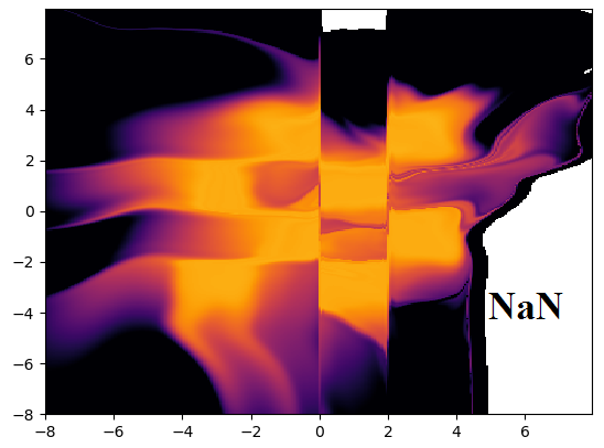
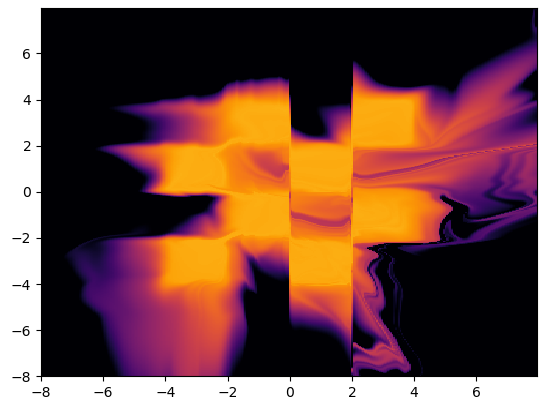
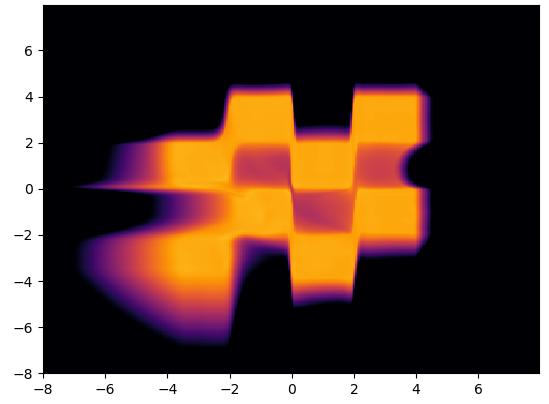
In addition to the reconstruction error in Figure 2 (main body of the paper), we visualize the learned density function for the models above in Figure 9. Most importantly, the instability a the affine model is clearly visible in the NaN density values outside the data domain. The more stable affine model with the modified scaling does not exhibit this failure, but still appears to learn a density with large slopes. The residual flow on the other hand learns a more stable distribution. Lastly, we note that the trained models on this 2D data were deliberately large to emphasize failures even in a low dimensional setting.
Appendix D DETAILS FOR OOD AND SAMPLE EVALUATION EXPERIMENTS
The examples from each OOD dataset were normalized such that pixel values fell into the same range as each model was originally trained on: for Glow, and for Residual Flows. The OOD datasets were adopted from previous studies including those by Hendrycks and Gimpel (2016); Liang et al. (2017). Extended results are shown in Table 5. The pre-trained models we used for OOD evaluation were from the official Github repositories corresponding to the respective papers. The pre-trained Glow model used convolutions.
| CIFAR-10 | SVHN | Uniform | Rademacher | Places |
|---|---|---|---|---|
![[Uncaptioned image]](/html/2006.09347/assets/ood/glow/cifar_test_orig_0.png) |
![[Uncaptioned image]](/html/2006.09347/assets/ood/glow/svhn_test_orig_0.png) |
![[Uncaptioned image]](/html/2006.09347/assets/ood/glow/uniform_orig.png) |
![[Uncaptioned image]](/html/2006.09347/assets/ood/glow/rademacher_orig.png) |
![[Uncaptioned image]](/html/2006.09347/assets/ood/glow/places_orig.png) |
![[Uncaptioned image]](/html/2006.09347/assets/ood/glow/cifar_test_recons_0.png) |
![[Uncaptioned image]](/html/2006.09347/assets/ood/glow/svhn_test_recons_0.png) |
![[Uncaptioned image]](/html/2006.09347/assets/ood/glow/uniform_recons.png) |
![[Uncaptioned image]](/html/2006.09347/assets/ood/glow/rademacher_recons.png) |
![[Uncaptioned image]](/html/2006.09347/assets/ood/glow/places_recons.png) |
Details for Training Glow
This section details the Glow models trained with the Flow/MLE objective reported in Section 4.1.2. These models have slightly different hyperparameters than the pre-trained Glow models. The controlled hyperparameters are listed in Table 6.
| Hyperparameter | Value |
|---|---|
| Batch Size | 64 |
| Learning Rate | 5e-4 |
| Weight Decay | 5e-5 |
| Optimizer | Adamax |
| Flow Permutation | Reverse |
| # of Layers | 3 |
| # of Blocks per Layer | 32 |
| # of Conv Layers per Block | 3 |
| # of Channels per Conv | 512 |
Details for Evaluating Glow
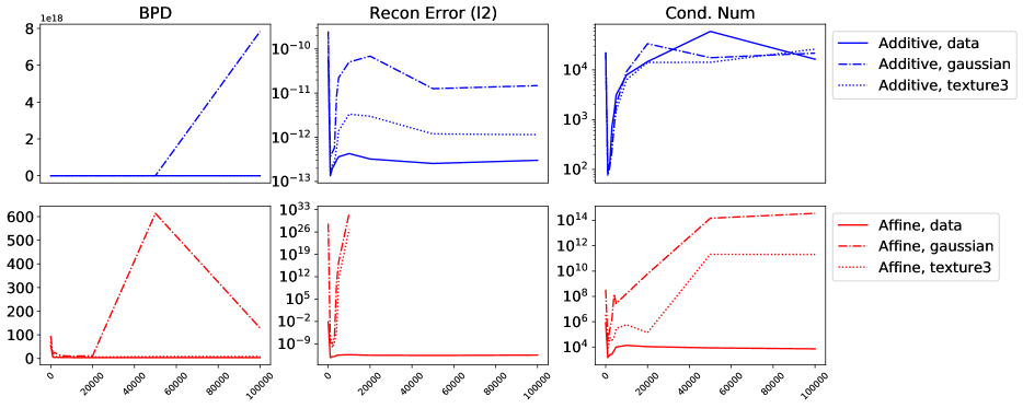
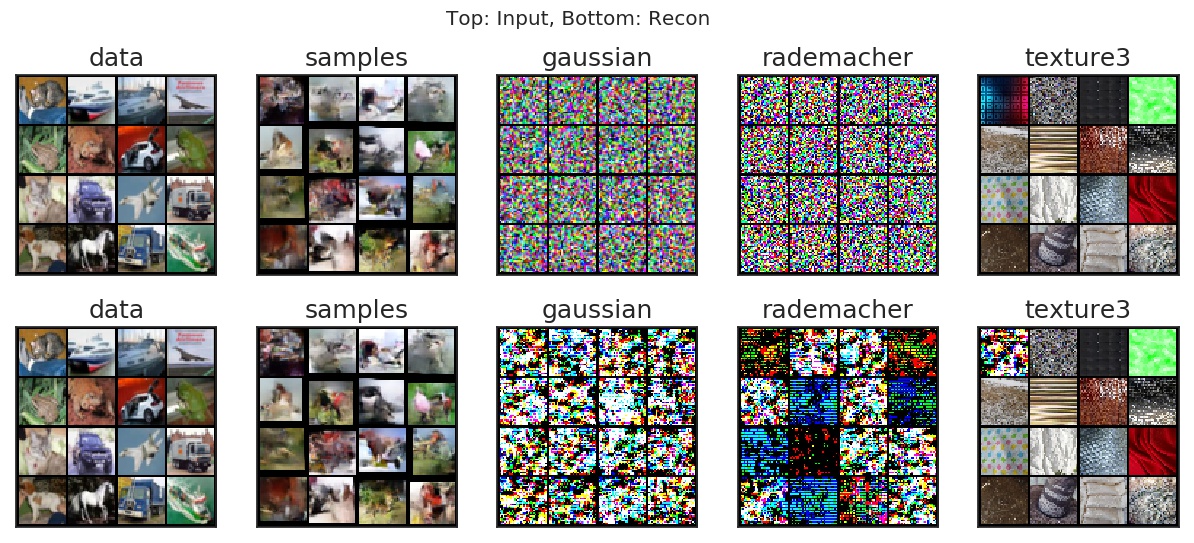
Stability statistics reported included reconstruction errors and condition numbers (Figure 10). Reconstruction error reported is the pixel-wise distance measured in the range. Input and reconstruction pairs are visualized in Figure 11. Condition numbers are computed numerically as follows: 1. gradient w.r.t. each dimension of the network output is computed sequentially to form the Jacobian, 2. SVD of the Jacobian is computed using “numpy.linalg.svd”, 3. the reported condition number is the ratio of the largest to smallest singular value.
Appendix E Non-Invertibility in Data Distribution
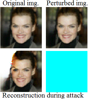
In this section we expose non-invertibility in the data distribution by optimizing within the dequantization distribution of a datapoint to find regions that are poorly reconstructed by the model. Note that the inputs found this way are valid samples from the training distribution. We performed this analysis with three NFs trained on CelebA64 with commonly-used 5-bit uniform dequantization: 1) affine Glow with standard sigmoid scaling; 2) affine Glow model with modified scaling in ; and 3) a Residual Flow. Starting from an initial training datapoint , we optimized in input-space to find a perturbed example that induces large reconstruction error using Projected Gradient Descent (Madry et al., 2018):
| (11) |
where is determined by the amount of uniform dequantization, see Appendix E.1 for details. As shown in Figure 12, this attack reveals the instability of affine models and underlines the stability of Residual Flows (Chen et al., 2019). To conclude, we recommend Residual Flows for a principled application of NFs.

E.1 Experimental Details of Invertibility Attack
In order to probe the invertibility of trained flow models over the entire data distribution, we trained three INN models on CelebA64 (with 5-bit dequantization) using the residual flows repository and the corresponding hyperparameter settings555from https://github.com/rtqichen/residual-flows/blob/master/train_img.py. For completeness, we provide the hyperparameters in the Table 7.
| Hyperparameter | Value |
|---|---|
| Batch Size | 64 |
| Learning Rate | 1e-3 |
| Weight Decay | 0 |
| Optimizer | Adam (ResFlow), Adamax (Affine) |
| Warmup iter | 1000 |
| Inner Dim | 512 |
| Num Blocks | 16-16-16-16 |
| ActNorm | True |
| Activation | Swish (ResFlow), ELU (Affine) |
| Squeeze First | True |
| Factor Out | False |
| FC end | True |
| Num Exact Terms | 8 |
| Num Trace Samples | 1 |
| Padding Distribution | uniform |
For evaluation we used the checkpoint obtained via tracking the lowest test bits-per-dimension. As a summary, we obtained the following three models:
-
1.
An affine coupling model with standard sigmoid scaling for the elementwise function from Eq. 4, which results in a scaling in .
-
2.
A modified affine coupling model with a scaling in by a squashed sigmoid.
- 3.
To explore the data distribution, we first need to consider the pre-processing step that is used to turn the quantized digital images into a continuous probability density: dequantization, see e.g. (Ho et al., 2019) for a recent discussion on dequantization in normalizing flows. Here we used the common uniform dequantization with 5-bit CelebA64 data, which creates noisy samples:
where . Thus, around each training sample there is a uniform distribution which has equal likelihood under the data model. If we explore this distribution with the invertibility attack below, we can guarantee by design that we stay within the data distribution. This is fundamentally different to the classical setting of adversarial attacks (Szegedy et al., 2013), where it is unknown if the crafted inputs stay within the data distribution.
These models were then probed for invertibility with the data distribution using the following attack objective:
| (12) |
where , and was selected from the training set of CelebA64. By using this constraint, we thus make sure that we explore only within the data distribution. The optimization was performed using projections to fulfill the constraint and by signed gradient updates as:
with and .
In addition to the visual results in Figure 12, we present visual results from the Residual Flow model in Figure 13. For this model, we have to remark one important aspect: due to memory constraint on the used hardware (NVIDIA GeForce GTX 1080, 12 GB memory), we could only use 5 fixed-point iterations for the inverse of the i-ResNet (Behrmann et al., 2019), since computing backprop through this iteration is memory intensive. This is why, we observe visible reconstruction errors in Figure 13, which are due to a small number of iterations as the reconstruction on the right with more iterations shows. However, we note that the comparison is not entirely fair since the gradient-based attack has only access to the 5-iteration inverse, while for affine models it has access to the full analytical inverse. Thus, future work should address this issue e.g. by considering non-gradient based attacks.
Appendix F EXPERIMENTAL DETAILS FOR 2D TOY REGRESSION
In this section we provide experimental details for the 2D toy regression experiment in Section 4.2.
Data.
To generate the toy data, we sampled input-target pairs distributed according to the following multivariate normal distributions:
| (13) | ||||
| (14) |
We used 1e-24 so that we are essentially mapping onto a 1D subspace.
Model.
We used an affine Glow model with reverse permutations and ActNorm (Kingma and Dhariwal, 2018), where each block was a multi-layered perceptron (MLP) with two hidden layers of 128 units each and ReLU activations. We trained the model in full-batch mode using Adam with fixed learning rate 1e-4 for 40,000 iterations.
Additional Results.
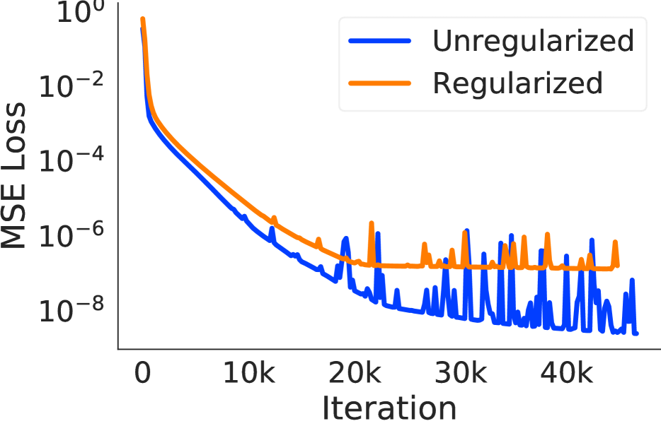
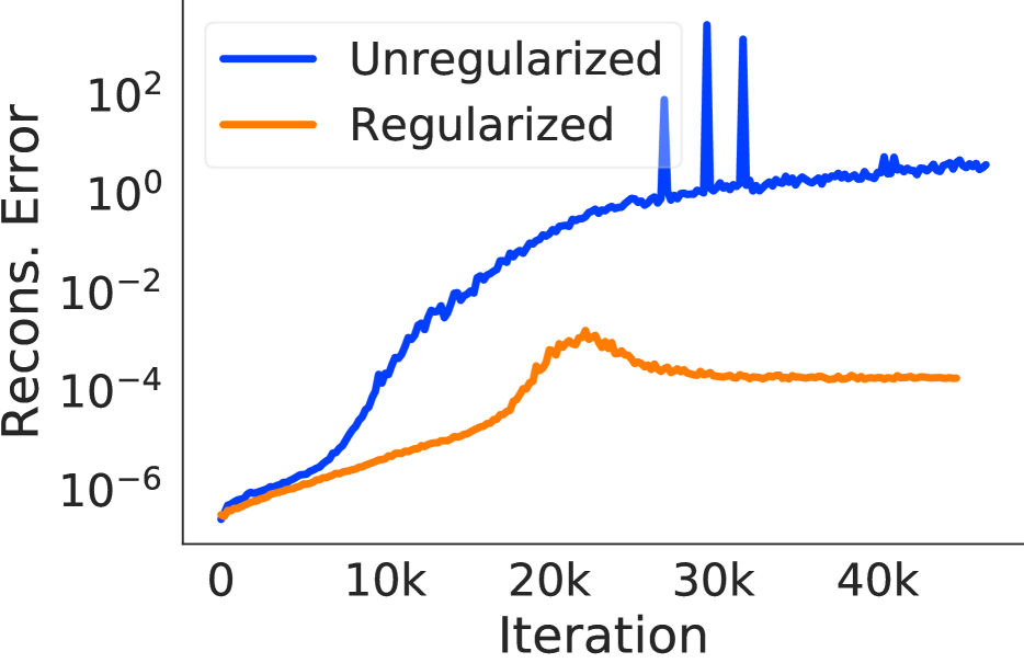
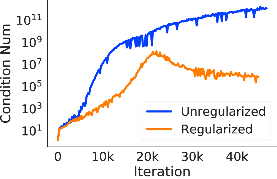
Figure 14 compares the mean squared error (MSE) loss, numerical reconstruction error, and condition number of the unregularized and regularized Glow models trained on this toy task. The regularized model adds the normalizing flow objective with a small coefficient of 1e-8. Here we see that the regularized model still achieves low MSE, while remaining stable with reconstruction error more than four orders of magnitude smaller than the unregularized model, and a condition number six orders of magnitude smaller.
Appendix G EXPERIMENTAL DETAILS FOR CLASSIFICATION EXPERIMENTS
In this section we provide details on the experimental setup for the classification experiments in Section 4.2, as well as additional results. We used the PyTorch framework (Paszke et al., 2019) for our INN implementations. All experiments were run on NVIDIA Titan Xp GPUs.
Experimental Setup.
All the additive and affine coupling-based models we used have the same architecture, that consists of 3 levels, 16 blocks per level, and 128 hidden channels. Each level consists of a sequence of residual blocks that operate on the same dimensionality. Between levels, the input is spatially downsampled by in both width and height, while the number of channels is increased by . Each block consists of a chain of convolutions. Because the dimension of the output of an INN is equal to that of the input (e.g., we have a 3072-dimensional feature space for CIFAR-10 images), we use a projection layer () to map the feature representation to 10 dimensions representing class logits. We trained the models on CIFAR-10 for 200 epochs, using Adam with initial learning rate 1e-4, decayed by a factor of 10 at epochs 60, 120, and 160 (following (Zhang et al., 2019)). We used standard data normalization (transforming the data to have zero mean and unit variance), and data augmentation (random cropping and horizontal flipping). The hyperparameters we used are summarized in Table 8.
| Hyperparameter | Value |
|---|---|
| Batch Size | 128 |
| Learning Rate | 1e-4 (decayed by 10x at epochs ) |
| Weight Decay | 0 |
| Optimizer | Adam(, ) |
| # of Layers | 3 |
| # of Blocks per Layer | 16 |
| # of Conv Layers per Block | 3 |
| # of Channels per Conv | 128 |
| Method | Coeff. | Inv? | Test Acc | Recons. Err. | Cond. Num. | Min SV | Max SV |
|---|---|---|---|---|---|---|---|
| Add. C, None | 0 | ✓ | 89.73 | 4.3e-2 | 7.2e+4 | 6.1e-2 | 4.4e+3 |
| Add. C, FD | 1e-3 | ✓ | 88.34 | 5.9e-4 | 4.3e+1 | 2.1e-1 | 9.1e+0 |
| Add. C, FD | 1e-4 | ✓ | 89.10 | 9.3e-4 | 2.0e+2 | 9.8e-2 | 2.0e+1 |
| Add. C, FD | 5e-5 | ✓ | 89.71 | 1.1e-3 | 3.0e+2 | 8.7e-2 | 2.6e+1 |
| Add. C, NF | 1e-3 | ✓ | 84.11 | 5.5e-4 | 6.5e+3 | 3.2e-2 | 2.1e+2 |
| Add. C, NF | 1e-4 | ✓ | 88.65 | 6.5e-4 | 4.7e+3 | 3.4e-2 | 1.6e+2 |
| Add. C, NF | 1e-5 | ✓ | 89.52 | 9.9e-4 | 1.7e+3 | 3.9e-2 | 6.6e+1 |
| Aff. S, None | 0 | ✗ | 87.64 | NaN | 9.9e+13 | 1.7e-12 | 1.6e+2 |
| Aff. S, FD | 1e-3 | ✓ | 86.85 | 2.0e-5 | 4.0e+1 | 1.8e-1 | 7.1e+0 |
| Aff. S, FD | 1e-4 | ✓ | 88.14 | 3.1e-5 | 1.2e+2 | 1.1e-1 | 1.3e+1 |
| Aff. S, FD | 5e-5 | ✓ | 88.13 | 3.9e-5 | 1.8e+2 | 9.6e-2 | 1.7e+1 |
| Aff. S, NF | 1e-3 | ✓ | 80.75 | 3.1e-5 | 2.2e+4 | 2.0e-2 | 4.4e+2 |
| Aff. S, NF | 1e-4 | ✓ | 87.87 | 2.3e-5 | 5.8e+3 | 3.1e-2 | 1.8e+2 |
| Aff. S, NF | 1e-5 | ✓ | 88.31 | 2.8e-5 | 8.5e+2 | 3.7e-2 | 3.2e+1 |
| Aff. C, None | 0 | ✗ | 89.07 | Inf | 8.6e+14 | 1.9e-12 | 1.7e+3 |
| Aff. C, FD | 1e-3 | ✓ | 88.24 | 6.0e-4 | 4.2e+1 | 2.0e-1 | 8.4e+0 |
| Aff. C, FD | 1e-4 | ✓ | 89.47 | 9.6e-4 | 1.6e+2 | 9.6e-2 | 1.5e+1 |
| Aff. C, NF | 1e-3 | ✓ | 83.28 | 7.0e-4 | 1.0e+4 | 3.6e-2 | 3.8e+2 |
| Aff. C, NF | 1e-4 | ✓ | 88.64 | 8.6e-4 | 9.6e+3 | 2.7e-2 | 2.6e+2 |
| Aff. C, NF | 1e-5 | ✓ | 89.71 | 1.3e-3 | 2.2e+3 | 3.5e-2 | 7.7e+1 |
Regularization Hyperparameters.
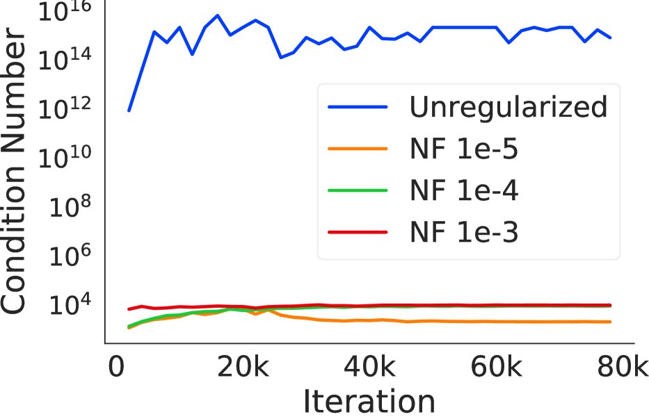
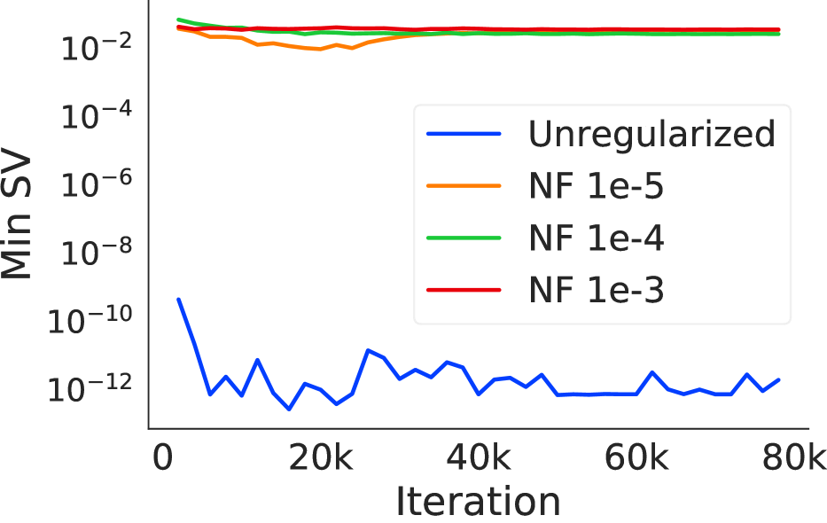
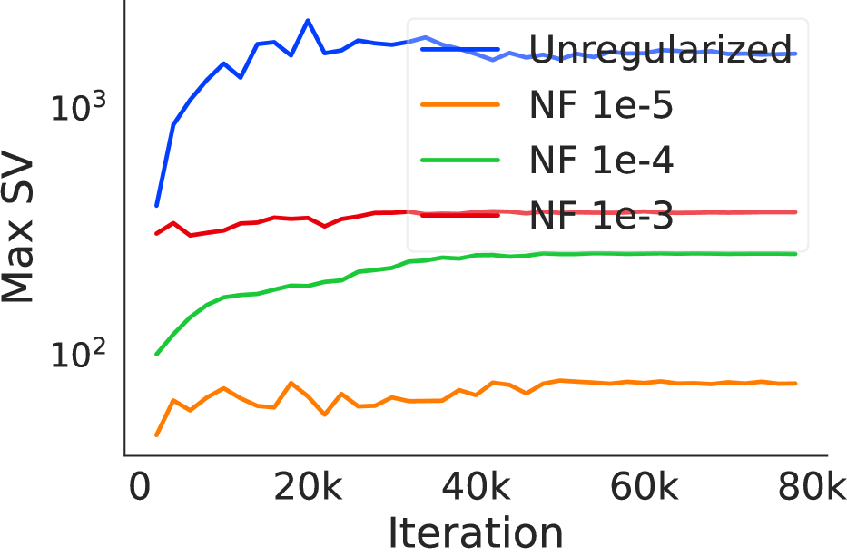
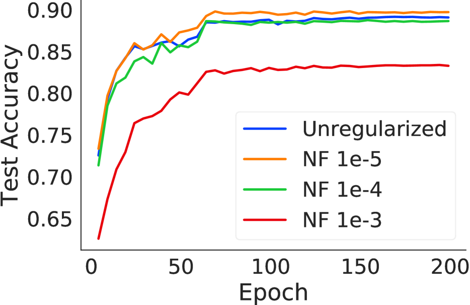
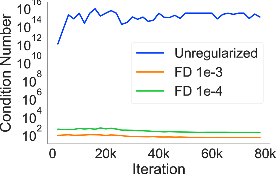
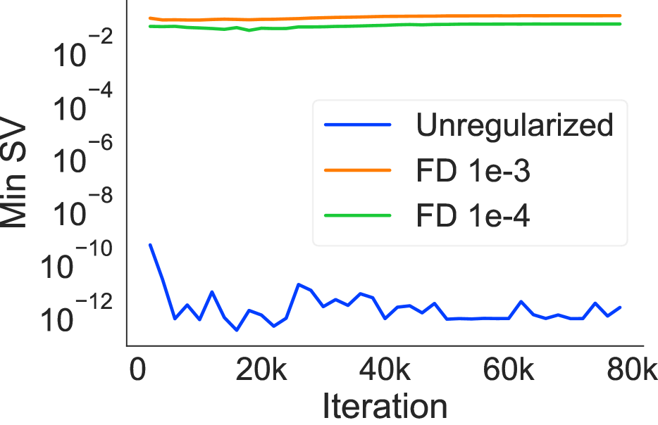
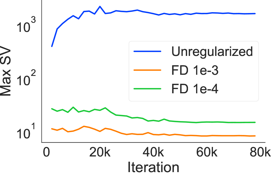
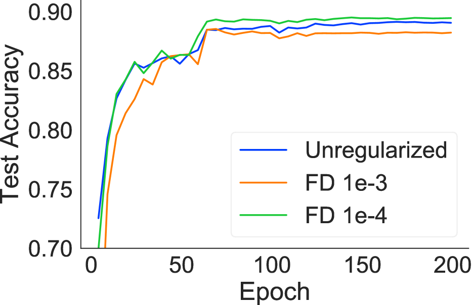
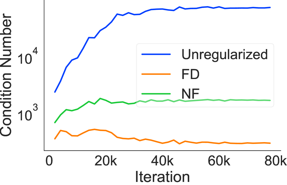
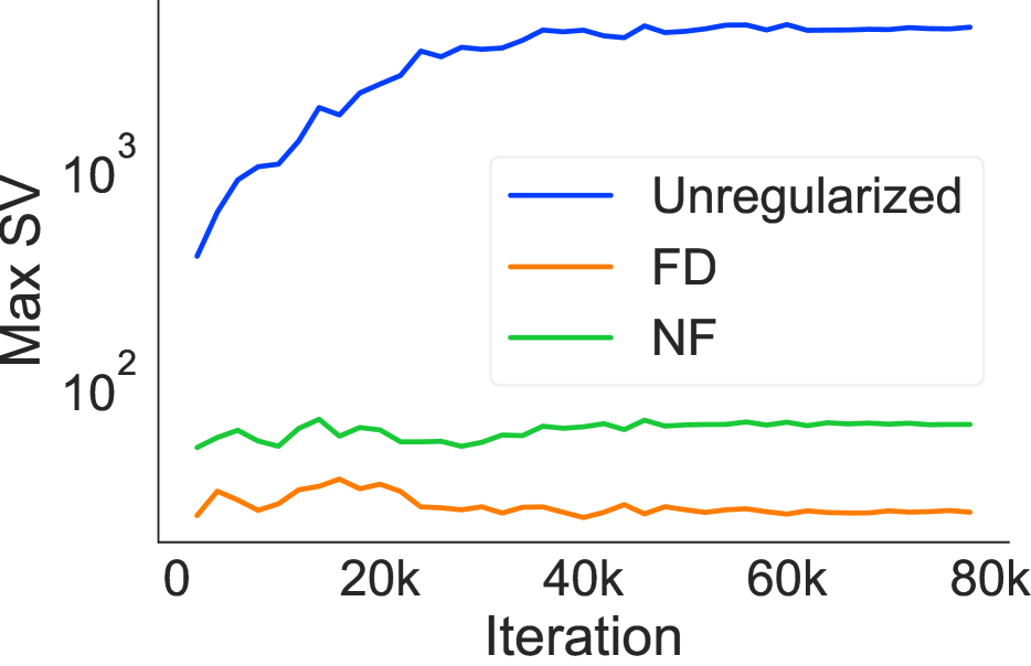
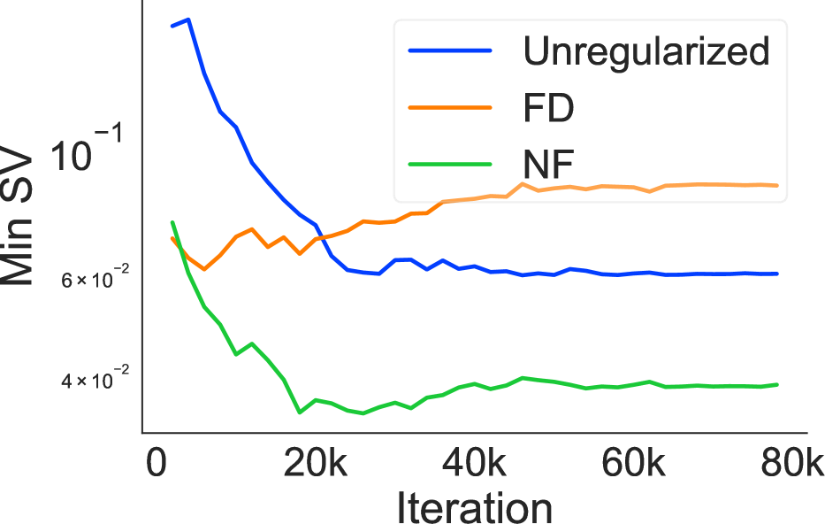
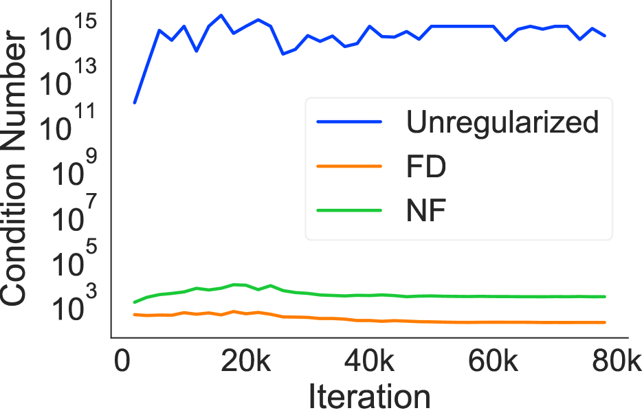
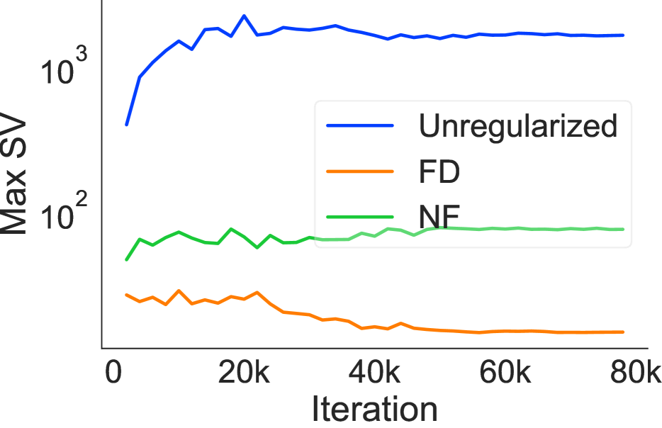
We performed grid searches to find suitable coefficients for the regularization schemes we propose. In particular, we searched over coefficients 1e-3, 1e-4, 1e-5 for the normalizing flow regularizer, and 1e-3, 1e-4, 5e-5 for bi-directional finite-differences (FD) regularization. The effects of different regularization strengths are summarized in Table 9. We also plot the condition numbers, maximum/minimum singular values, and test accuracies while training with different coefficients for the normalizing flow objective (Figure 15) and bi-directional FD (Figure 16). For both regularization methods, larger coefficients (e.g., stronger regularization) yield more stable models with smaller condition numbers, but too large a coefficient can harm performance (i.e., by hindering model flexibility). For example, using a large coefficient (1e-3) for the normalizing flow objective substantially degrades test accuracy to 83.28%, compared to 89.07% for the un-regularized model.
Extended Results.
We provide an extended version of Table 2 (from the main paper) in Table 10, where we also include additive and affine models with shuffle permutations. Figures 17 and 18 visualize the stability during training using each regularizer, for additive and affine models, respectively.
| Model | Regularizer | Inv? | Test Acc | Recons. Err. | Cond. Num. | Min SV | Max SV |
|---|---|---|---|---|---|---|---|
| Additive Shuffle | None | ✓ | 88.35 | 1.1e-4 | 2.1e+3 | 2.9e-2 | 6.0e+1 |
| FD | ✓ | 88.49 | 5.4e-5 | 7.0e+2 | 5.3e-2 | 3.7e+1 | |
| NF | ✓ | 88.49 | 2.2e-5 | 1.1e+3 | 3.0e-2 | 3.3e+1 | |
| Additive Conv | None | ✓ | 89.73 | 4.3e-2 | 7.2e+4 | 6.1e-2 | 4.4e+3 |
| FD | ✓ | 89.71 | 1.1e-3 | 3.0e+2 | 8.7e-2 | 2.6e+1 | |
| NF | ✓ | 89.52 | 9.9e-4 | 1.7e+3 | 3.9e-2 | 6.6e+1 | |
| Affine Shuffle | None | ✗ | 87.64 | NaN | 9.9e+13 | 1.7e-12 | 1.6e+2 |
| FD | ✓ | 88.14 | 3.1e-5 | 1.2e+2 | 1.1e-1 | 1.3e+1 | |
| NF | ✓ | 88.31 | 2.8e-5 | 8.5e+2 | 3.7e-2 | 3.2e+1 | |
| Affine Conv | None | ✗ | 89.07 | Inf | 8.6e14 | 1.9e-12 | 1.7e+3 |
| FD | ✓ | 89.47 | 9.6e-4 | 1.6e+2 | 9.6e-2 | 1.5e+1 | |
| NF | ✓ | 89.71 | 1.3e-3 | 2.2e+3 | 3.5e-2 | 7.7e+1 |
Finite Differences Regularization.
Computational Efficiency of Regularizers.
Most invertible neural networks are designed to make it easy to compute the log determinant of the Jacobian, needed for the change-of-variables formula used to train flow-based generative models. For coupling-based INNs, the log determinant is particularly cheap to compute, and can be done in the same forward pass used to map . Thus, adding a regularizer consisting of the weighted normalizing flow loss does not incur any computational overhead compared to standard training.
Bi-directional finite differences regularization is more expensive: memory-efficient gradient computation involves a forward pass, an inverse pass, and a backward pass. The forward regularizer adds an additional overhead to these computations because it requires the previous computations not only for clean , but also for noisy . The inverse regularizer also passes two variables and through its computations, which are: an inverse pass to compute the reconstruction, a forward pass to re-compute activations of the inverse mapping and the backward pass through the inverse and forward. However, in practice the cost can be substantially reduced by applying regularization only once per every iterations of training; we found that and performed similarly to in terms of their stabilizing effect, while requiring only a fraction more computation (e.g., 1.26 the computation when ) than standard training. See the wall-clock time comparison in Table 11.
We also experimented with applying the FD regularizer only to the inverse mapping, and while this can also stabilize the inverse and achieve similar accuracies, we found bi-directional FD to be more reliable across architectures. Applying regularization once every 10 iterations, bi-FD is only 1.06 slower than inverse-FD. As the FD regularizer is architecture agnostic and conceptually simple, we envision a wide-spread use for memory-efficient training.
| Method | Time per Epoch (s) | Overhead |
|---|---|---|
| Unregularized | 281.0 | 1 |
| Reg. Every 1 | 854.1 | 3.04 |
| Reg. Every 5 | 406.6 | 1.45 |
| Reg. Every 10 | 354.6 | 1.26 |
Comparing True and Memory-Saving Gradients.
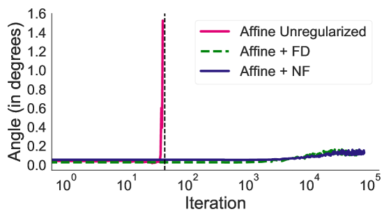
For the gradient angle figure in the introduction (Section 1), we used additive and affine Glow models with convolutions. To create that figure, we first trained both models with exact (non-memory-saving) gradients, and saved model checkpoints during training; then, we loaded each checkpoint and computed the angle between the true and memory-saving gradients for a fixed set of 40 training mini-batches and plotted the mean angle. We did not train those models with memory-saving gradients, because this would have made it impossible to train the unstable affine model (due to the inaccurate gradient).
Figure 19 shows a similar analysis, comparing the angles between true and memory-saving gradients for an affine model trained with and without regularization. The regularized models were trained with memory-saving gradients, while the unregularized model was trained with standard backprop. Similarly to the introduction figure, we saved model checkpoints throughout training, and subsequently loaded the checkpoints to measure the angle between the angles for the 40 training mini-batches, plotting the mean angle. Applying either finite differences or normalizing flow regularization when training the affine model keeps the angles small, meaning that the memory-saving gradient is accurate, and allowing us to train with this gradient.
Appendix H OUTLOOK ON BI-DIRECTIONAL TRAINING WITH FLOW-GAN
Experimental Details.
Table 12 summarizes the hyperparameters for all models trained in our Flow-GAN experiments. The INN architecture in this experiment is similar to those described in Appendix D. Table 12 lists hyperparameters changed for this experiment.
| Hyperparameter | Value |
|---|---|
| Batch Size | 32 |
| Learning Rate (Generator) | 5e-5 |
| Learning Rate (Discriminator) | 5e-5 |
| Weight Decay (Both) | 0 |
| Optimizer | Adam(, ) |
| # of Layers | 3 |
| # of Blocks per Layer | 8 |
| # of Conv Layers per Block | 3 |
| # of Channels per Conv | 128 |
The prior is a standard normal. One extra hyperparameter here is the weight of the MLE loss (which is considered as a regularizer here). The discriminator had 7 convolution layers, each is regularized by Spectral normalization (Miyato et al., 2018) and using the LeakyReLU activation. The depth of the convolution layers are (64, 64, 128, 128, 256, 256, 512). The discriminator is further regularized with gradient penalty (Gulrajani et al., 2017) and optimized using the binary cross entropy GAN loss.
Stability at Data.
Similarly to the results in the classification Section 4.2, when a flow is trained as a GAN, it suffers from non-invertibility even at training points. This is easily explained as the INN generator is never explicitly trained at the data points, but only receives gradients from the discriminator.
Using the MLE objective on the generator alleviates this issue. It increases the stability at the data-points, and makes training more stable in general, as discussed in section 3.3.2. This is exactly the FlowGAN formulation proposed in (Grover et al., 2018). See Table 13 for a comparison of test-set likelihoods and sample quality. In contrast to (Grover et al., 2018), we find additive Glow models trained with the GAN objective alone to be very unstable. We used a weighing of 1e-3 for the MLE loss for the reported results here. One suspicion is that the introduced ActNorm in the Glow architecture is causing extra instability.
Originally, one hypothesis was that the astronomically large BPD when trained as a GAN was caused by instability. This is likely incorrect. Even for stable runs (with a smaller, more stable architecture) that had no reconstruction errors and small condition numbers, the model still assigns incredibly large BPDs.
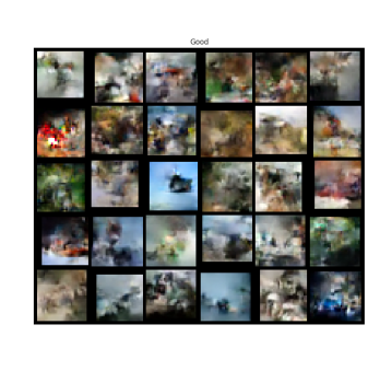
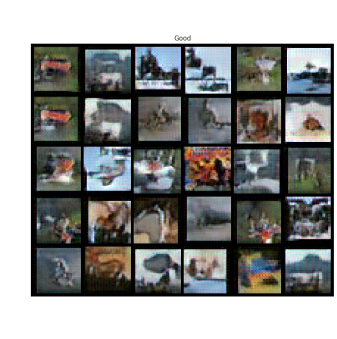
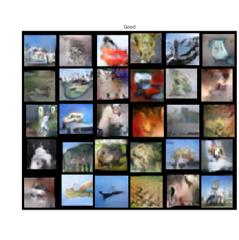
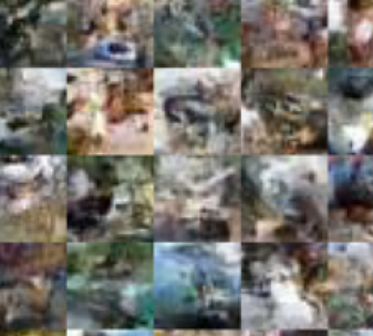
Our FlowGAN models strike a good balance between good test-set likelihood and improving sample quality. See Figure 20 for samples. The FlowGAN samples show better “objectness” and do not have the high-frequency artifacts shown in the MLE samples.
Unfortunately, given the fact that the GAN-only objective assigns unexplained BPDs, it’s still unclear whether interpreting the BPDs for the FlowGAN in the same way as MLE models is recommended.
| Objective | Inception Score | BPD |
|---|---|---|
| MLE | 2.92 | 3.54 |
| GAN | 5.76 | 8.53 |
| FlowGAN | 3.90 | 4.21 |
| - | FID | BPD |
| MLE | 790 | 3.77 |
| GAN* | 850 | Inf |
| FlowGAN | 420 | 4 |
| MLE | GAN | FlowGAN |
|---|---|---|
 |
 |
 |
 |
 |
 |
