Dynamic Window-level Granger Causality of Multi-channel Time Series

Abstract

Granger causality method analyzes the time series causalities without building a complex causality graph. However, the traditional Granger causality method assumes that the causalities lie between time series channels and remain constant, which cannot model the real-world time series data with dynamic causalities along the time series channels. In this paper, we present the dynamic window-level Granger causality method (DWGC) for multi-channel time series data. We build the causality model on the window-level by doing the F-test with the forecasting errors on the sliding windows. We propose the causality indexing trick in our DWGC method to reweight the original time series data. Essentially, the causality indexing is to decrease the auto-correlation and increase the cross-correlation causal effects, which improves the DWGC method. Theoretical analysis and experimental results on two synthetic and one real-world datasets show that the improved DWGC method with causality indexing better detects the window-level causalities.

Keywords Causal inference  $\cdot$ Time Series  $\cdot$ Nonlinear Autoregressive  $\cdot$ Dynamic window-level

1 Introduction

Time series data is the data with the pre-defined time or sequencial order [1] and is widely used in multifarious real-world applications, such as signal processing [2], economics [3], control theory [4], etc. Typical tasks for time series data include indexing, clustering, classification, and regression [5]. Among the time series tasks, the causal reasoning task is at the top level of cognitive reasoning [6] and is getting rid of the nature of the correlation fitting for traditional statistical machine learning and deep learning, which is nevertheless at the bottom level. Due to the natural implication of the temporal precedence, the time-series data therein encapsulates both empirical experiences of the trends, but also the prior knowledge of causalities between different channels [7].

Granger [8] first used the statistical hypothesis test to decide whether one time series channel is useful to predict another, which is known as Granger causality (GC) and widely used in various applications. Lynggarrd and Walther [9] proposed the dynamic interaction models based on the classical ‘LWF Markov property’ for chain graphs [10, 11]. Pearl and Robins [12] put forward the ‘back door’ temporal causal conditions and extend the traditional Granger causality to the temporal sequences. Dahlhaus and Eicher [13] discussed an alternative approach that defined the graph according to the ‘AMP Markov property’ of [14]. Eichler [15] adopted the mixed graph constraints, derived from ordinary time series, and used a single vertex and directed edges to represent the component series and the causal relationship respectively.

The traditional Granger causality methods are limited to the predictive capability of the autoregressive model (AR) which only used the linear models. Eichler [7] re-described the problems when transferring the Granger causality to the nonlinear version: 1) the aggregation of the time-varying coefficients overtime required by Granger causality tests, and 2) the instability of the causal structure. Chen et al. [16] used a delay embedding to get an extended nonlinear version of Granger Causality. Later, Sun [17] proposed to use the RKHS kernel embeddings to get the nonlinearity.

The aforementioned works assume that the Granger causalities remain unchanged between time series channels throughout time [18], which is called “channel-level Granger causality”. In the real world, the time series data is becoming massive, complicated and uncertain, and the causality relations would change along with the sliding windows of the time series data (see Fig. 1 as an example).

According to the philosopher David Hume, “cause and effect have temporal precedence[19]”. This acquiesced that causality or precedence itself is in relation with, and even change dynamically with time. In this sense, the constant causality assumption[18] is not always true and the purpose of this assumption for the traditional Granger causality is to take sufficient long (but definitely not necessary) time series in order to distinguish the random correlation and causalities [18]. Some attempts on dynamic causalities have already been done in neural science: the “dynamic causal modeling” (DCM) method detects the real-time dynamic causal relationships among neuron clusters in the brain. However, it’s by interfering the “input-state-ouput” framework in brain and observing its response and cannot directly extract causalities without the model that have relationships like brain [20].

(a) Traditional Channel-level Granger causality

(b) Dynamic Window-level Granger Causality

Figure 1: Window-level causality(right) is to analyze dynamic changing causalities on sliding windows on time series. While channel-level method assume causalities remain constant between time series channels(left)

1.1 Our Proposal

In this paper, we present the dynamic window-level Granger causality method (DWGC) for time series data. To capture the dynamic causality relations, we relax the sufficiently long time series assumption and build the causality model on the sliding windows of the time series. To capture the non-linearities in the time series forecasting, we use nonlinear autoregressive model to fit the time series and extract the nonlinear features. Based on the NAR model predictions, an F-test is used by comparing the prediction results of NAR models on the sliding windows. Further, to reduce the possible fluctuations of auto-correlation on window-level F-test, we introduce a causality-index matrix and optimize the corresponding causality indexing loss accuracy. We theoretically prove that: 1) the traditional Granger causality is a special case of our dynamic window-level Granger method; 2) the dynamic window-level Granger method outperforms the traditional Granger causality with the causality indexing.

In the experiments, we implement our DWGC model on three datasets, two synthetic data, and one real-world meteorological data (with prior knowledge). For the synthetic data, we use AR/NAR simulator to generate several synthetic time series. For the real-world meteorological dataset, we examine the obtained dynamic causalities between the El-Nino values and the East Asian monsoon over the seasonal cycle which was already examined in the previous literature.

In summary, the contributions of this paper are as follows:

• We propose and solve a new task: identify dynamic window-level causality of multi-channel time series.

• We theoretically show that the proposed dynamic window-level Granger causality model contains the traditional Granger causality as a special case and is more accurate with the causality indexing.

• We conduct the numerical experiments on two synthetic and one real-world datasets and the proposed dynamic window-level Granger method shows that this method can find the accurate window causalities.

2 Related Works

2.1 Preliminaries of Granger Causality

Granger causality is the most widely used causality analysis method for time series data [8], which is also the main focus of this paper. We use the following sequence to represent the stationary sequence of random variables, i.e, the time series data $i$:

$${(Y_{i1},Y_{i2},Y_{i3},\cdots,Y_{it},\cdots)},$$ (1)

where ${Y_{i,t}}$ and $Y_{<t}$ are the series data $i$ at and before time $t$. Granger causality defines ${Y_{i}}$ as the cause of ${Y_{j}}$, if the series $i$ provides useful information when predicting the future values of series $j$:

$$E_{t}(g_{j}(Y_{j,t+1}|Y_{j,<t},Y_{i,<t}))\neq E_{t}(g_{j}(Y_{j,t+1}|Y_{j,<t})),$$ (2)

where $E_{t}$ is the accuracy expectation of the prediction function $g$ on time series. Besides, the premise of (2) is that channels i and j meet the “backdoor condition[21]”, that is, there is no common interference from confounding factors of other channel. Also, it’s worth pointing out that Granger causality is still a type of statistical association as it does not go through the necessary causal identification process of [6].

Traditional Granger causality methods use a linear auto-regressive model for $g$. In this paper, we use the double-headed arrow to express the Granger causality $i$ to $j$:

$$Y_{i}{\Longrightarrow}Y_{j}.$$ (3)

Granger causality is considered as a “precedence” according to the informal fallacy “Post hoc ergo propter hoc”. This Latin fallacy means “after this, therefore because of this”. It shows the causality as the precedence that the follow-up event is caused by the previous event.

The linear Granger causality can be extended to the nonlinear version for better fitting nonlinear sequences. In [22], a non-linear prediction model, such as the multi-layer perceptron, is defined as $Y_{jt}=g_{j}(Y_{1,<t},\cdots,Y_{d,<t})$. Then, we can say $Y_{i}{\Longrightarrow}Y_{j}$, if for all $Y_{i,<t}^{{}^{\prime}}\neq Y_{i,<t}$:

$$g_{j}(Y_{1,<t},...,Y_{i,<t},...,Y_{d,<t})\neq g_{j}(Y_{1,<t},...,Y_{i,<t}^{{}^{\prime}},...,Y_{d,<t}).$$ (4)

$g$ is represented as MLP(Multilayer Perceptron)/LSTM(Long Short-Term Memory) network in [22]. Both linear and nonlinear Granger causality method assumes that the causalities between time series are constant and cannot model the dynamic causalities that lie in the real world.

2.2 Improvements of Granger method to generalize to the nonlinearity/window level

More recently, the deep neural networks are used to get nonlinear Granger causalities [23, 24, 25, 26, 22, 27]. In these previous works, the neural network is used to replace the original AR model for sequence fitting and prediction, and then causal reasoning methods (such as counterfactual principle, Granger method) are brought into the framework of neural network.

On the other hand, Granger’s approach has been extended from channel level to window level. Sezen Cekic[28] use KL(Kullback-Liebler) divergence instead of F-test to extend the window-level Granger method, first in neuroscience.

To both deal with nonlinearity and window-level challenges, sliding window method is common, which is also applicable in Granger causality situation. The neuroscience Granger causality extended to the nonstationary case by wavelet transforms or multitapers on sliding window by Mattia F.Pagnotta[29], whereas as far as we know, there is no related method that can address both the nonlinear and the window-level problems in a wider application scenario.

2.3 Causal Graph for Time Series

Besides the Granger causality, the causal graph is another way to identify the causality between different channels of time series [25]. The causal graph model can be built based on vector autoregressive Granger analysis(VAR), the generalized additive models(GAMs) [30] or the certain pre-assumed regression models [31]. However, the causal graph is limited to the structure itself to extend to the dynamic window-level for time series data.

2.4 Distinction between causal effects and noise

In each window, it is a subtle topic to distinguish whether the time series trend variations are due to the causal effects or random noise. On the one hand, commonly-used time series anomaly detection methods barely consider causal effects when detecting different abnormal noises. In [32], although an attempt is made to use anomaly detection to divide the actual sequence into two parts: steady-state structure part and causal influence part, the second part does not make a practical distinction between noise and causality. On the other hand, the traditional Granger causality method keeps the ignorance of noise intervention in most cases.

3 Dynamic Window-level Granger Causality

3.1 Naive Dynamic Window-level Granger Causality Model

To detect dynamic window-level causality between two data series $Y_{i}$ and $Y_{j}$, we first use a sliding window of length $k$ on the same time position $t$ of the two series:

$$\{Y_{i,t},Y_{i,t+1},\cdots,Y_{i,t+k-1}\},~{}~{}~{}\{Y_{j,t},Y_{j,t+1},\cdots,Y_{j,t+k-1}\}.$$ (5)

Aiming at finding the dynamic causality at the window level, we consider two forms of time-series fitting on each sliding window $(t,t+k-1)$: predicting the future values of one series with and without the information from the other series channel, which are similarly used in the traditional Granger causality method. Compared to equation (2), we use nonlinear auto-regressive(NAR) model, and use mean square error(MSE)[33] as $E_{t}$ to measure two accuracies:

$$L_{1}=E(\mathrm{MSE}({\hat{Y}_{i,t\sim t+k-1}},Y_{i,t\sim t+k-1}|Y_{i,<t})),$$ (6)

$$L_{2}=E(\mathrm{MSE}({\hat{Y}_{i,t\sim t+k-1}},Y_{i,t\sim t+k-1}|Y_{i,<t},Y_{j,<t}),$$ (7)

where $\hat{Y}_{i,t\sim t+k-1}$ means prediction on the sliding window $(t,t+k-1)$. We determined the existence of causality by setting a reasonable threshold $\epsilon$ based on the value of $F_{statistic}$:

$$F_{statistic}=\frac{L_{1}}{L_{2}}.$$ (8)

The causality exists between the series $i$ and $j$ on the sliding window $(t,t+k-1)$ if $F_{statistic}$ is larger than the pre-defined threshold $\epsilon(>1)$.

3.2 Dynamic Window-level Causality Model

In the naive version of the dynamic window-level causality method, auto-correlation would easily occur with the disturbances of the NAR model along the time series. To address this problem, we introduce the causality indexing matrix $\Phi$ in our method and then decompose the causal effects and auto-regressive correlations. The original time series includes two factors: the cross-correlation and the auto-correlation. By converting to windows-level, the auto-correlation becomes more unstable and conceals the causal effects in the cross-correlation. The auto-regression correlations in one single series is represented in $L_{1}$ in Eqn. (6), intuitively, when auto-correlation is unusually large on a local window, it will make the window-level f-test result higher than the normal value, which may affect the overall accuracy of the model, or affect the overall recall rate conversely. We use a scale function $h$ to scale down the auto-correlation and adopt a corresponding causal indexing matrix $\Phi$, to measure the likelihood that each time point will serve as a starting or ending point for causality. The indexing loss as

$$Loss=\sum_{m,i}\mathrm{KL}\left(\Phi_{m}^{i},\{{}{h(\hat{Y}_{i,q}-Y_{i,q})^{2}}\}\right),q=m,m+1,...m+k-1,$$ (9)

where $\hat{Y},Y$ are the prediction results and the real series respectively, $i$ is the channel index and $m$ is the starting point of each sliding window with length $k$. By optimizing this loss, $\Phi$ can be used to scale down the original series data $Y$ with large auto-correlations as:

$$\begin{bmatrix}A_{i,t}\\ A_{i,t+1}\\ ...\\ A_{i,t+k-1}\end{bmatrix}=\Phi^{i}_{t\sim t+k-1}*\begin{bmatrix}Y_{i,t}\\ Y_{i,t+1}\\ ...\\ Y_{i,t+k-1}\end{bmatrix},i=1,2,...d,$$ (10)

where $*$ is Hadamard product. With the causality indexing $\Phi$, we scale down the auto-correlation and get the reweighted series $A$. In this paper, we use the following scaling function:

$$h=(\alpha-\tanh(\cdot)),\alpha>1.$$ (11)

It is worth mentioning that the selection of the scaling function $h$ can be further improved by certain regularization item and this will be analyzed in the Appendix C.

Data: Multi-channel time series $Y_{t}$ and predefined F-test threshold $\epsilon$.

initialization, $\Phi$ set to all-one;

while NAR forecast loss and causal indexing loss converge do

       Reweight original time series using causal index matrix $\Phi$ via Eqn. (10);

       Train an NAR model using reweighted series $A_{t}$ as the input;

       Finding dynamic causalities via Eqn. (12);

       In all the window pairs with the detected causalities, optimize Loss (9) to optimize $\Phi$;

      

end while

Position causality from window-level to point-to-point level by (14).

Result: Dynamic window level causalities

Algorithm 1 Framework of our method(DWGC)

We test the dynamic window-level causality using the causality indexing as:

$$F_{statistic}=\frac{L_{1}}{L_{2}}=\frac{E(MSE({\hat{A}_{i,t\sim t+k-1}},A_{i,t\sim t+k-1}|A_{i,<t}))}{E(MSE({\hat{A}_{i,t\sim t+k-1}},A_{i,t\sim t+k-1}|A_{i,<t},A_{j,<t}))}.$$ (12)

We further obtain the starting and ending points in the sliding window by finding the maximum of the index matrix:

$$Y_{i,t_{1}} \stackrel{{\scriptstyle}}{{\Longrightarrow}} Y_{j,t_{2}}$$ (13)

$$\{t_{1},t_{2}\}=\mathop{\max} \{\Phi_{t_{1}}^{i}+\Phi_{t_{2}}^{j}|t_{1}<t_{2},~{}~{}~{}t_{1},t_{2}\in(t,t+k-1)\}.$$ (14)

In our dynamic window-level Granger causality (DWGC) method, we alternatively optimize the NAR forecasting model and the causality index loss Eqn. (9) and extract causalities after the two loss function converge. The final procedure is outlined in Algorithm 1.

4 Theoretical Analysis of DWGC

In this section, we give the theoretical analysis of the proposed dynamic window-level Granger causality method(DWGC). We first give the formulation preparation and then prove that 1) DWGC without causality indexing is a special case of the traditional Granger causality method and 2) DWGC with causality is more accurate than the traditional Granger causality method for those causality pairs.

We consider the sample pairs whose expectation of $F_{statistic}$ $F_{0}$ is larger than the predefined threshold $\epsilon$. These samples are expected to be tested as causal in the traditional Granger causality method.

4.1 Formulation Preparation

The time series observations $Y_{t}$ can be decomposed into two parts: real data and Gaussian noise. For simpilicity, We use the standard Gaussian for the random noise and get the following decomposition of the time series $i$:

$$Y_{i}=Y_{i}^{\text{real}}+\gamma_{i},\gamma\sim\mathcal{N}(0,1)$$ (15)

We denote the model predictions of the NAR model with/without another causality source series channel $j$ as $\hat{Y}_{i}$ and $\hat{Y}_{i|j}$.

Then the F-statistic of Eqn. (8), i.e, the ratio between the MSE of the NAR models with/without the channel $j$, can be turned to

$$F_{statistic}= \frac{L_{1}}{L_{2}}=\frac{{\sum_{t}{(\hat{Y}_{it}-Y^{\text{real}}_{it}-\gamma)}^{2}}}{{\sum_{t}{(\hat{Y}_{it|j}-Y^{\text{real}}_{it}-\gamma)}^{2}}}$$ (16)

$$= \frac{\sum_{t}{(\hat{Y}_{it}-Y^{\text{real}}_{it})}^{2}+\sum_{t}\gamma_{it}^{2}-2\sum_{t}\gamma_{it}(\hat{Y}_{it}-Y^{\text{real}}_{it})}{\sum_{t}{(\hat{Y}_{it|j}-Y_{it}^{\text{real}})}^{2}+\sum_{t}\gamma_{it}^{2}-2\sum_{t}\gamma_{it}(\hat{Y}_{it|j}-Y_{it}^{\text{real}})}$$

$$\approx \frac{\sum_{t}{(\hat{Y}_{it}-Y^{\text{real}}_{it})}^{2}+\sum_{t}\gamma_{it}^{2}}{\sum_{t}{(\hat{Y}_{it|j}-Y_{it}^{\text{real}})}^{2}+\sum_{t}\gamma_{it}^{2}}.$$

The square sum of the standard normal noise $\sum_{t}\gamma_{t}^{2}$ follows the chi-square distribution $\chi^{2}(k)$, where $k$ is the length of the sliding window. When the window length $k$ is reasonably large, the third term in the above formulation can be omitted. The details of the omitting derivation can be seen in Appendix (A).

4.2 DWGC without causality indexing degenerates to Traditional Granger causality

We analyze the distribution of the F-statistic of the naive DWGC and give the following result.

Theorem 1.

For the time series sliding windows with causalities, the probability of F-statistic of naive DWGC larger than the threshold $P(F(k)>1)$ is a monotone increasing function for $k$ in the case where $k$ is sufficiently large.

We prove the above theorem using the series expansion of $P(F(k)=\epsilon)$ on each $k$, and leave the details in Appendix B.

This theorem can be intuitively analyzed from the expression of the F-statistic in Eqn.(16): for numerator, $E(\sum_{t}{(\hat{Y}_{it}-Y^{\text{real}}_{t})}^{2}+\sum_{t}^{k}\gamma_{t}^{2})=k(E(\hat{Y}_{it}-Y^{\text{real}}_{t})^{2}+1)$, for denominator, $E(\sum_{t}{(\hat{Y}_{it|j}-Y^{\text{real}}_{t})}^{2}+\sum_{t}^{k}\gamma_{t}^{2})=k(E(\hat{Y}_{it|j}-Y^{\text{real}}_{t})^{2}+1)$, so when k is sufficiently large, Eqn.(16) can be approximate to $\frac{(\hat{Y}_{it}-Y^{\text{real}}_{t})^{2}+1}{(\hat{Y}_{it|j}-Y^{\text{real}}_{t})^{2}+1}(>1)$.

Without the causal indexing, the larger the sliding window length $k$ is, the more accurate the DWGC method without the causality indexing would be. When $k$ goes to infinity, the DWGC method without the causality indexing degenerate to the traditional causality method.

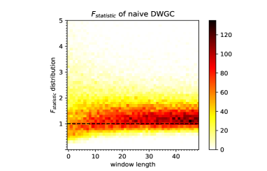
Fig. 2(left) is the scatter heatmap of F-statistic of the naive DWGC method. The x-axis is the sliding window length and the y-axis is the is the value of the F-statistic. This figure is done based on an experiment for a synthetic AR-simulation data with causalities, which will be further illustrated in the experiment section. As can be seen from the results, the expectation of F-statistic of naive DWGC is monotone increasing for the window length $k$.

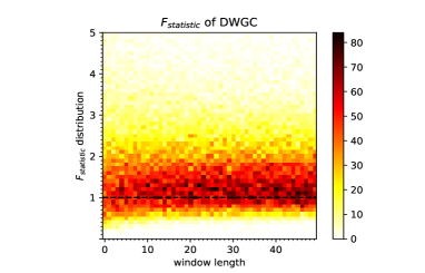
Figure 2: The scatter heatmap of $F_{statistic}$ results from the multiple tests. The tested data are the synthetic AR simulation data pairs with causalities. The causality analysis methods are naive DWGC without causal indexing (left) and DWGC with causal indexing (right). The black dashed line is the causality threshold $\epsilon=1$. The area above the black dashed line is causal and the area below is not.

4.3 DWGC with causality indexing generate more accurate causality result

In this section, we give the sufficient condition of $\Phi$ to improve our DWGC method.

Theorem 2.

Certain causality-indexing $\Phi$ exists to improve the accuracy of our DWGC causality result on each window length k.

We prove the above theorem by adopting the series expansion of $F_{statistic}$ in (1), and take the increasing of each series after adding $\Phi$ as a sufficient condition to improve our DWGC effect.

Existence of $\Phi$ can be intuitively illustrated as follows. The important reason why the Eqn. (16) is unstable before adding $\Phi$ is that $(\hat{Y}_{it}-Y^{\text{real}}_{t})$,$\gamma_{t}$ and $(\hat{Y}_{it|j}-Y^{\text{real}})$ are all independently distributed Gaussian variables, so it gives a unstable influence on $F_{statistic}$. However, with the causal indexing $\Phi$, an causal reweighting method is to assign specific weights to establish correlation between each item by $\Phi$. For example, when $(\hat{Y}_{it}-Y^{\text{real}}_{t})$ is observed to be significantly out of the normal range, we give $\Phi$ to both scale down the fitting error and noise, so as to offset the negative effect of abnormal fitting values on time point t on the whole $F_{statistic}$.

Besides, Eqn. (9) give another view to explain the existence of $\Phi$. During the experiment, we can include this theoretical sufficient condition into the regularization term of loss function(9) to help iterative optimization. In a word, our DWGC method’s effect can be improved by $\Phi$ satisfying certain condition. Concrete form of this sufficient condition is shown in Appendix C.

5 EXPERIMENTS

In this section, we present the empirical result comparisons of the dynamic window-level causality method.

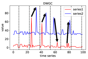
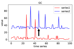
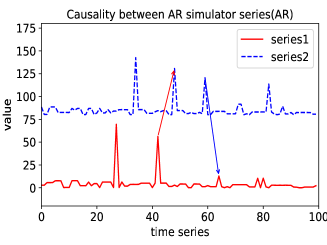
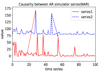
Figure 3: The partial simulation data in AR/NAR experiment, the blue/red curve represents two channels of the time series, arrows represent causal relationships. The starting position of each arrow is at the point when m1(m2) takes an abnormally large value. In this partial display, some of mutations are caused by causal effects and some are abnormal noise. It is easy to confuse causal effects with noise by direct observation.

5.1 Results on Synthetic AR/NAR Simulation Dataset

We first construct the dataset using AR and NAR simulations. The construction details are as follows: 1) The linear AR simulation construction: We simulate two linear AR time series with a random lag value randomly picked from one to nine. The initial value of $T_{1},T_{2}$ is $T_{i,t}=\left\{\begin{aligned} t&~{}&\ t\in[1,5]\\ 11-t&~{}&\ t\in[6,10]\end{aligned}\right.,$ i=1,2.

$$T_{1,t}=m_{1}T_{2,t-lag}+0.02\mathcal{N}(0,1)$$ (17)

$$T_{2,t}=m_{2}T_{1,t-lag}+0.02\mathcal{N}(0,1),$$

$$m_{1},~{}m_{2}=\begin{cases}0.9&\text{p=0.95}\\ 10&\text{p=0.05}\end{cases}$$

2) The non-linear AR simulation construction: we simulate two non-linear AR time series with a random lag value randomly picked from one to nine. The initial value of $T_{1},T_{2}$ is $T_{i,t}=\left\{\begin{aligned} t&~{}&\ t\in[1,5]\\ 11-t&~{}&\ t\in[6,10]\end{aligned}\right.,$ i=1,2.

$$T_{1,t}=m_{1}\mathrm{Re}(\sqrt{{T_{2,t-lag}}^{2}-1})+N(0,1)$$ (18)

$$T_{2,t}=m_{2}\mathrm{Re}(\sqrt{{T_{1,t-lag}}^{2}-1})+N(0,1)$$

$$T_{3,t}=\sin(0.1t),$$

where $m_{1}=\left\{\begin{aligned} 10&~{}&\ T_{3,t}>0.9\\ 0.9&~{}&\ T_{3,t}<0.9\end{aligned}\right.,m_{2}=\left\{\begin{aligned} 10&~{}&\ T_{3,t}<-0.9\\ 0.9&~{}&\ T_{3,t}>-0.9\end{aligned}\right.$, $lag\in\{1,2,3,...9\}$, and $\mathrm{Re(\cdot)}$ takes the real part of the square root.

5.1.1 Experimental Results

A fragment of the AR/NAR simulation data is shown in Fig. 3 (left: AR and right: NAR). The arrows means the lag relation between the two series and we consider them as the ground truth of the dynamic causalities.

For the two AR/NAR simulation datasets, we first pre-process the data to make sure that the time series are stationary. The reweight function $g$ for causaling index (Eqn. (11)) as $(\frac{6}{5}-\tanh(\cdot))$, $\epsilon=1$. Step length is taken as the window length.

Table 1: Causality Recall of naive DWGC and DWGC(ours) on two AR/NAR simulation datasets

dataset		10	20	30	100
AR simulations	naive DWGC	0.48(0.06)	0.49(0.05)	0.77(0.03)	0.77(0.02)
	DWGC(ours)	0.72(0.03)	0.72(0.05)	0.80(0.03)	0.88(0.05)
NAR simulations	naive DWGC	0.59(0.06)	0.60(0.06)	0.73(0.06)	0.87(0.03)
	DWGC(ours)	0.84(0.05)	0.90(0.02)	0.84(0.08)	0.88(0.02)

Table 2: Causality Accuracy of naive DWGC and DWGC(ours) on two AR/NAR simulation datasets

dataset		10	20	30	100
AR simulations	naive DWGC	0.22(0.06)	0.43(0.05)	0.82(0.03)	0.90(0.02)
	DWGC(ours)	0.23(0.03)	0.45(0.05)	0.84(0.03)	0.92(0.05)
NAR simulations	naive DWGC	0.42(0.07)	0.76(0.09)	0.93(0.06)	1.00(0.04)
	DWGC(ours)	0.44(0.05)	0.79(0.04)	0.94(0.05)	1.00(0.03)

On each window, if we detect $F_{statsitic}>1$ with at least a set of causality pairs in this window, our causality extraction on this window is successful. In this case, we calculate the accuracy/recall of the naive DWGC and DWGC methods on the data points with causalities in Table 1. As can be seen from the results, for the recall/accuracy rate, DWGC method performs better than naive DWGC method when the sliding window length is generally small. Besides, The recall rate of naive DWGC method increases with the sliding window length, which certifies the theoretical results.

5.2 Results on Climate Dataset for ElNiño

In this part, we verify the DWGC model on a real climate dataset, which has widely recognized seasonal causalities.

5.2.1 Academia Knowledge of ElNiño and monsoon

The climate academia already have the following definition on ElNiño: a climate phenomenon in the Pacific equatorial belt where the ocean and atmosphere interact with each other and lose their balance [34]. While monsoon generally refers to the seasonal conversion of atmospheric circulation and precipitation in tropical and subtropical areas, and two parameters are used to measure its strength: OLR(Outgoing Longwave Radiation) and MKE(Monsoon Kinetic Energy).

The causal interaction between ENSO and the east Asian monsoon has been extensively explored:

1. The causality $\text{ENSO}\Longrightarrow\text{MKE/OLR}$ and $\text{ENSO}\Longrightarrow\text{MKE/OLR}$ exists, especially in autumn and winter.

2. The reverse causal effect $\text{MKE/OLR}\Longrightarrow\text{ENSO}$ and $\text{MKE/OLR}\Longrightarrow\text{ENSO}$ also exists in spring and summer, the strength change of the Asian monsoon will in turn trigger the formation of ENSO event.

However, in recent decades, the accuracy of this ENSO-based causal model seems to have a downward trend. Therefore, the DWGC method would be helpful for analyzing the data with dynamic causalities like this.

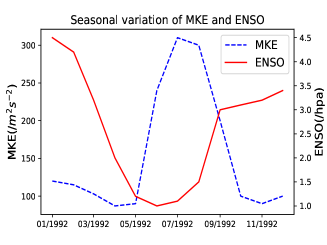
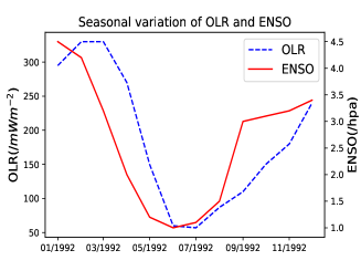
Figure 4: Original data of MKE/OLR and ENSO.

5.2.2 Experiment

We used ENSO and Asian monsoon data in 1992 and the series trends can be seen from the part of the raw data in Fig. 4. We take the first four months as training data and the rest as the testing data [35]. For the comparison with prior knowledge, we selected the window length as one month.

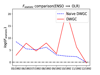
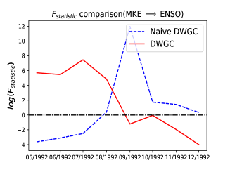
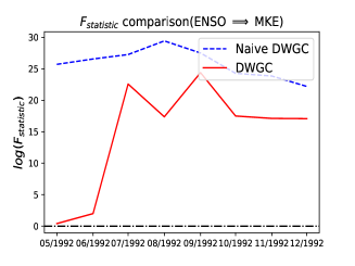
Figure 5: $F_{statistic}$ from ENSO to MKE/OLR using GC(naive DWGC) and DWGC method. In GC, there is a causal relationship between ENSO and MKE & OLR in most months, but there is no obvious trend of causal change on the whole. In our method DWGC, on the basis of detecting the causal relationship $\text{ENSO}\Longrightarrow\text{MKE}$ and $\text{ENSO}\Longrightarrow\text{OLR}$, we further find that both the causal relationship in autumn and winter(Oct-Dec) is obviously stronger than that in spring and summer(May-Aug)(confirms the priori meteorology conclusion[36]).

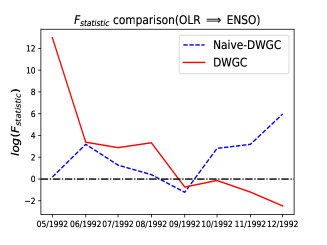
Figure 6: $F_{statistic}$ from MKE/OLR to ENSO using GC(naive DWGC) & DWGC method. Compared with GC method, DWGC can successfully detect reverse causality $ENSO\Longrightarrow MKE$ in spring and summer(May)(confirms the prior meteoroogy[37]).

We use our model(DWGC) to judge the window-level causalities between ENSO and Asian monsoon in every month. In Fig. 5, we show the F-statistic values of every month of DWGC and naive DWGC without causality indexing for two series (ENSO,MKE) and (ENSO, OLR). The x-axis is the month-time and the y-axis is the log-scale F-statistic value. The black dot-dash line with value zero is the F-statistic threshold. For naive DWGC without causality indexing, the causality between ENSO and two parameters of east Asian monsoon(MKE,OLR) can be successfully detected, but the difference of causality between May-Aug(spring and summer) and Aug-Dec(autumn and winter) is not significant. However, in our DWGC method, after detecting the basic causal relationship of ENSO $\Longrightarrow$ MKE and ENSO $\Longrightarrow$ OLR, we further find that the causal relationship in autumn and winter is more significant than that in spring and summer in both of them with the larger F-statistic values. This significant causality variation detected by our DWGC is consistent with the academic knowledge[36].

In Fig. 6, we show the F-statistic values of every month of DWGC and naive DWGC for two series (MKE,ENSO) and (OLR,ENSO), with the same figure axis and F-statistics threshold of Fig. 5. For naive DWGC without causality indexing, we detect the causality $\text{MKE}\Longrightarrow\text{ENSO}$ in Sep-Dec(autumn and winter) and the causality $\text{OLR}\Longrightarrow\text{ENSO}$ in May-Jul(spring and summer) and Oct-Dec(autum and winter). However, in our DWGC method, we detect the causality $\text{MKE}\Longrightarrow\text{ENSO}$ and $\text{OLR}\Longrightarrow\text{ENSO}$ in May-Aug(spring and summer). Compared to the naive DWGC method, our causalities results of DWGC are more close to the academia knowledge[37].

6 Conclusions and Future Work

In this paper, a new task is proposed to detect the window-level dynamic causal relationship between the time series data. By directly conducting the F-test on comparing the window level forecasting predictions with/without the cause channel, the naive DWGC can detect the window-level causalities. This naive DWGC is a special case of the traditional Granger method and is not accurate enough especially when the sliding window length is not large enough. We introduce a technique called “causal indexing” to reweight the original time series. The purpose of this technique is to decrease the effects of the auto-correlation noise and increase the cross-correlation causal effects. The improved DWGC method is proved to have better causality detection accuracies. causalities detection accuracies. As far as we know, this paper is the first to propose and solve the new task of dynamic Granger causal relationship detection at the window level. In the experiments on two synthetic and one real datasets, we show that our DWGC method outperforms the traditional GC and the naive DWGC in sense of the causality detection accuracies.

The dynamic causalities detected by DWGC is restricted to the same sliding window of every time series. In the future, we are interested in detecting the dynamic causalities without prior knowledge of the sliding window length and between the different sliding windows, and further analyzing the effect of step length for the dynamic causality detection.

Appendix A The Simplification of F-test result

Lemma 1.

If k is large enough, $\sigma_{0}=\sigma_{0}(\hat{Y}_{t}-Y_{t}^{real})$, we have the probability density function:

$$f_{\frac{{\sum_{t}^{k}\gamma_{t}(\hat{Y}_{t}-Y^{real}_{t})}}{\sum_{t}^{k}\gamma_{t}^{2}}}(x)=O(e^{-\frac{e^{6}k}{2(\sigma_{0}^{2}+1)}x^{2}})$$ (19)

Proof.

Due to that the sum and product of Gaussian variables still satisfy Gaussian distribution N(0,$\sigma_{0}$)(ignore the systematic error). We have:

$$s_{1}=\sum_{i=1}^{k}\gamma_{i}(\hat{Y}-Y_{real}) \sim\frac{1}{\sqrt{2\pi k(\sigma_{0}^{2}+1)}}e^{-\frac{s_{1}^{2}}{2k(\sigma_{0})^{2}+1)}}$$ (20)

$$s_{2}=\sum_{i=1}^{k}\gamma_{i}^{2} \sim\frac{1}{2^{\frac{k}{2}}}e^{-\frac{s_{2}}{2}}s_{2}^{\frac{k}{2}-1}$$

$$s3=\frac{\sum_{i=1}^{k}\gamma_{i}(\hat{Y}-Y_{real})}{\sum_{i=1}^{k}\gamma_{i}^{2}} \sim\int_{0}^{+\infty}\frac{1}{2^{\frac{k}{2}}\tau(\frac{k}{2})\sqrt{2\pi k(\sigma_{0}^{2}+1)}}e^{-\frac{t^{2}s_{3}^{2}}{2k(\sigma_{0}^{2}+1)}-\frac{t}{2}}t^{\frac{k}{2}-1}dt$$

So

$$f(s_{3}) =\int_{0}^{+\infty}\sum_{n=0}^{+\infty}\frac{1}{2^{\frac{k}{2}}\tau(\frac{k}{2})\sqrt{2\pi k(\sigma_{0}^{2}+1)}}\frac{(-\frac{t^{2}x^{2}}{2k(\sigma_{0}^{2}+1)})^{n}}{n!}e^{-\frac{k}{2}}t^{\frac{k}{2}-1}dt$$ (21)

$$=\sum_{i=0}^{+\infty}\frac{(-1)^{n}x^{2n}}{2^{\frac{k}{2}}\tau(\frac{k}{2})\sqrt{2\pi k(\sigma_{0}^{2}+1)}n!2^{n}k^{n}(\sigma_{0}^{2}+1)^{n}}e^{-\frac{t}{2}}t^{\frac{k}{2}-1+2n}dt$$

$$=\sum_{i=0}^{+\infty}\frac{(-1)^{n}2^{n}x^{2n}\tau(2n+\frac{k}{2})}{\tau(\frac{k}{2})\sqrt{2\pi k(\sigma_{0}^{2}+1)}n!k^{n}(\sigma_{0}^{2}+1)^{n}}$$

$$\sim\frac{1}{\sqrt{2\pi(\sigma_{0}^{2}+1)}}\sum_{n=0}^{+\infty}\frac{(-\frac{e^{6}k}{2(\sigma_{0}^{2}+1)})^{n}x^{2n})}{n!}$$

$$\sim\frac{1}{\sqrt{2\pi(\sigma_{0}^{2}+1)}}e^{-\frac{e^{6}k}{2(\sigma_{0}^{2}+1)}x^{2}}$$

Its convergence rate is significantly faster than that of the Gaussian variable in the same form(the rate is $e^{6}k^{2}$), which can be ignored as it tends to zero in most cases. ∎

Appendix B Proof of Theorem 1

B.1 Preliminary

Nash efficiency coefficient[38] is often used to evaluate the performance of simulation prediction, which is expressed as:

$$Nash=1-\frac{\sum_{t=1}^{n}(\hat{Y}_{t}-Y_{t})^{2}}{\sum_{t=1}^{n}(Y_{t}-E(Y_{t}))^{2}},Nash_{\Phi}=1-\frac{\sum_{t=1}^{n}(\hat{Y}^{\Phi}_{t}-\phi Y_{t})^{2}}{|E(\phi)|^{2}\sum_{i=1}^{n}(Y_{t}-E(Y_{t}))^{2}}$$

if out model’s Nash efficiency coefficient is stable, that is: $Nash=Nash_{\Phi}$, we can get:

$$\sum_{t=1}^{n}(\hat{Y}^{\phi}_{t}(\hat{Y}^{\phi}_{t|j})-\Phi Y_{t})^{2}=|E(\phi)|^{2}\sum_{t=1}^{n}(\hat{Y}_{t}(\hat{Y}_{t|j})-Y_{t})^{2},$$

B.2

Proof.

$$f_{F_{statistic}}^{k}(\epsilon)=\sum_{i=0}^{\frac{k}{2}-1}(\frac{k}{2\sigma\sqrt{\epsilon_{0}}})^{k}\frac{C_{\frac{k}{2}-1}^{i}(\epsilon-1)^{i}\epsilon^{\frac{k}{2}-1-i}\frac{(\frac{k}{2})^{\frac{k}{2}}\tau(\frac{k}{2}+i)}{\tau(\frac{k}{2})[\frac{k}{2}(1+\frac{\epsilon-1}{\epsilon_{0}\sigma})]^{\frac{k}{2}+i}}(\frac{2\epsilon_{0}\sigma}{k(\epsilon+\epsilon_{0})})^{k-1-i}\tau(k-1-i)}{\tau(\frac{k}{2})^{2}}$$ (22)

Let’s call each series $g(\epsilon,k,i)$, so $f_{F_{statistic}}^{k}=\sum_{i=0}^{\frac{k}{2}-1}g(\epsilon,k,i)$. We recursively prove that $f_{F_{statistic}}^{k}$ is a monotonic function with respect to k(when k is greater than a certain value,$\epsilon>1$):

$$\frac{d(ln(g(\epsilon,k,i)))}{dk}= lnk+1-ln(2\sigma\sqrt{\epsilon_{0}})-\digamma(\frac{k}{2})-\frac{1}{2}\digamma(\frac{k}{2}-i)+\frac{1}{2}ln\epsilon+\frac{1}{2}\digamma(\frac{k}{2}+i)-$$ (23)

$$\frac{1}{2}ln(1+\frac{\epsilon-1}{\epsilon_{0}\sigma})-\frac{i}{k}+ln(\frac{2\epsilon_{0}\sigma}{\epsilon+\epsilon_{0}})+\digamma(k-1-i)-lnk-\frac{k-1-i}{k}$$

$$= ln(\frac{\sqrt{\epsilon_{0}}\sqrt{\epsilon}}{(\epsilon+\epsilon_{0})\sqrt{1+\frac{\epsilon-1}{\epsilon_{0}\sigma}}})+\frac{1}{k}+ln(\frac{2\sqrt{\frac{k}{2}+i}}{\sqrt{\frac{k}{2}-i}}\frac{(k-1-i)}{k})$$

For each $\epsilon>1$, if we can find $\alpha$, $i\in(\alpha k-1,\frac{1}{2}k-1)$, we have

$$\frac{2\sqrt{\epsilon_{0}\epsilon}}{(\epsilon+\epsilon_{0})\sqrt{1+\frac{\epsilon-1}{\epsilon_{0}\sigma}}}\frac{\sqrt{\frac{1}{2}+\alpha}}{\sqrt{\frac{1}{2}-\alpha}}(1-\alpha)>0,f_{statistic}^{k}(\epsilon)-\sum_{i=0}^{\alpha k-1}g(\epsilon,k,i)=o(1)$$ (24)

We can get $\frac{d(ln(g(\epsilon,k,i)))}{dk}>0$, so

$$g(\epsilon,k+2,i)>g(\epsilon,k+1,i)>g(\epsilon,k,i),\epsilon>1$$ (25)

Here comes to the conclusion:

$$f_{F_{statistic}}^{k}=\sum_{i=0}^{\frac{k}{2}-1}g(\epsilon,k,i)<\sum_{i=0}^{\frac{k}{2}}g(\epsilon,k,i)<\sum_{i=0}^{\frac{k}{2}}g(\epsilon,k+2,i)=f_{F_{statistic}}^{k+2}$$ (26)

∎

Also, we can give a simpler proof:

Proof.

$$P(F_{statistic}>1)$$ (27)

$$= P(\sum_{t}{(\hat{Y}_{it}-Y^{\text{real}}_{it})}^{2}>\sum_{t}{(\hat{Y}_{it|j}-Y^{\text{real}}_{it})}^{2})$$

$$= 1-\sum_{m=0}^{+\infty}\frac{\Gamma(k+m)(\frac{1}{\epsilon_{0}})^{\frac{k}{2}+m}}{(\frac{1}{\epsilon_{0}}+1)^{k+m}\Gamma(\frac{k}{2})\Gamma(\frac{k}{2}+m+1)}$$

Let’s take the derivative of the next term:

$${(\sum_{m=0}^{+\infty}\frac{\Gamma(k+m)(\frac{1}{\epsilon_{0}})^{\frac{k}{2}+m}}{(\frac{1}{\epsilon_{0}}+1)^{k+m}\Gamma(\frac{k}{2})\Gamma(\frac{k}{2}+m+1)})}^{{}^{\prime}}$$ (28)

$$= \phi(k+m)+\frac{1}{2}ln\frac{1}{\epsilon_{0}}-ln(\frac{1}{\epsilon_{0}}+1)-\phi(\frac{k}{2})-\phi(\frac{k}{2}+m+1)$$

$$<0$$

Therefore, equation (27) shows a single increasing trend with the increase of window length k. ∎

Appendix C Proof of Theorem 2

Lemma 2.

If ${\gamma_{t}}$ are k independent, circular symmetric complex Gaussian random variables with mean 0 and variance $\phi_{t}^{2}$, we have:

$$f_{\sum_{t=1}^{k}(\gamma_{t}^{2})}\left(x;k,\phi_{1}^{2},\ldots,\phi_{k}^{2}\right)=\sum_{t=1}^{k}\frac{e^{-\frac{x}{\phi_{t}^{2}}}}{\phi_{t}^{2}\prod_{j=1,j\neq t}^{k}\left(1-\frac{\phi_{j}^{2}}{\phi_{t}^{2}}\right)}\text{ for }x\geq 0$$ (29)

Theorem 3.

for each k, consider the window $\{\phi_{1},\phi_{2},..\phi_{k}\}$, the sufficient condition for $\int_{1}^{+\infty}f_{F_{statistic}}^{k,\Phi}(\epsilon)>\int_{1}^{+\infty}f^{k}_{F_{statistic}}(\epsilon)$ is:

$$\sum_{q=1}^{\frac{k}{2}}\frac{1}{\hat{\phi}_{q}^{2}\prod_{j\neq q}(1-\frac{\hat{\phi}_{j}^{2}}{\hat{\phi}_{q}^{2}})}>\frac{\tau(k-1)}{\tau(\frac{k}{2})^{2}}{(\frac{|E(\Phi)|^{2}}{\phi_{t}^{2}})}_{max},\hat{\phi}_{m}=\phi_{2m}=\phi_{2m-1}$$ (30)

Proof.

The $F_{statistic}$ can be represented as follows:

$$F_{statistic}\approx\frac{\sum_{t=1}^{k}{(\hat{Y}_{t}^{\Phi}-\phi_{t}Y_{t}^{real})}^{2}+\sum_{t=1}^{k}(\phi_{t}\gamma_{t})^{2}}{\sum_{t=1}^{k}{(\hat{Y}_{t|j}^{\Phi}-\phi_{t}Y_{t}^{real})}^{2}+\sum_{t=1}^{k}(\phi_{t}\gamma_{t})^{2}}$$ (31)

According to (31), two influencing factors-prediction error and noise-have changed. Using lemma 2, assume $\phi_{2m}=\phi_{2m-1}$, we do the series expansion $f^{k,\Phi}_{F_{statistic}}(\epsilon)=\sum_{q=1}^{\frac{k}{2}}\sum_{t=0}^{\frac{k}{2}-1}g_{2}(\epsilon,k,t,\phi_{q})$, so the sufficient condition for $\int_{\epsilon_{min}}^{\epsilon_{max}}f_{F_{statistic}}^{k,\Phi}(\epsilon)>\int_{\epsilon_{min}}^{\epsilon_{max}}f^{k}_{F_{statistic}}(\epsilon)$ is:

$$\sum_{q=1}^{\frac{k}{2}}g_{2}(\epsilon,k,t,\phi_{q})>g(\epsilon,k,t),$$ (32)

Comparing the series expansion of naive DWGC and DWGC, the sufficient condition of (32) is:

$\forall k,q:$

$$\sum_{q=1}^{\frac{k}{2}}\frac{k\tau(i+1)}{2\phi_{q}^{2}\prod_{j\neq q}(1-\frac{\phi_{j}^{2}}{\phi_{q}^{2}})(\frac{k}{2\phi_{q}^{2}}+\frac{k(\epsilon-1)}{2E|(\Phi)|^{2}\sigma\epsilon_{0}})^{i+1}|E(\Phi)|^{2i+2}}>\frac{(\frac{k}{2})^{\frac{k}{2}}\tau(\frac{k}{2}+i)}{(\frac{k}{2}+\frac{k(\epsilon-1)}{2\sigma\epsilon_{0}})^{\frac{k}{2}+i}\tau(\frac{k}{2})}$$ (33)

The sufficient condition can be converted to: :

$$\forall q,\sum_{q=1}^{\frac{k}{2}}\frac{k\tau(i+1)}{2\phi_{q}^{2}\prod_{j\neq q}(1-\frac{\phi_{j}^{2}}{\phi_{q}^{2}})(\frac{k|E(\Phi)|^{2}}{2\phi_{q}^{2}}+\frac{k(\epsilon-1)}{2\sigma\epsilon_{0}})^{i+1}}>\frac{(\frac{k}{2})^{\frac{k}{2}}\tau(\frac{k}{2}+i)}{(\frac{k}{2}+\frac{k(\epsilon-1)}{2\sigma\epsilon_{0}})^{\frac{k}{2}+i}\tau(\frac{k}{2})}$$ (34)

$$\forall q,\sum_{q=1}^{\frac{k}{2}}\frac{k\tau(i+1)}{2\phi_{q}^{2}\prod_{j\neq q}(1-\frac{\phi_{j}^{2}}{\phi_{q}^{2}})}>\frac{(\frac{k}{2}(\frac{(|E(\Phi)|^{2}}{\phi_{q}^{2}})_{max}+\frac{k(\epsilon-1)}{2\sigma\epsilon_{0}})^{i+1}(\frac{k}{2})^{\frac{k}{2}}\tau(\frac{k}{2}+i)}{(\frac{k}{2}+\frac{k(\epsilon-1)}{2\sigma\epsilon_{0}})^{\frac{k}{2}+i}\tau(\frac{k}{2})}\\$$ (35)

$$\forall q,\sum_{q=1}^{\frac{k}{2}}\frac{k\tau(i+1)}{2\phi_{q}^{2}\prod_{j\neq q}(1-\frac{\phi_{j}^{2}}{\phi_{q}^{2}})}>\frac{(\frac{k}{2}(\frac{(|E(\Phi)|^{2}}{\phi_{q}^{2}})_{max}+\frac{k(\epsilon-1)}{2\sigma\epsilon_{0}})(\frac{k}{2})^{\frac{k}{2}}\tau(\frac{k}{2}+i)}{(\frac{k}{2}+\frac{k(\epsilon-1)}{2\sigma\epsilon_{0}})^{\frac{k}{2}}\tau(\frac{k}{2})}\\$$ (36)

$$\forall q,\sum_{q=1}^{\frac{k}{2}}\frac{k}{2\phi_{q}^{2}\prod_{j\neq q}(1-\frac{\phi_{j}^{2}}{\phi_{q}^{2}})}> \frac{(\frac{k}{2}(\frac{(|E(\Phi)|^{2}}{\phi_{q}^{2}})_{max})(\frac{k}{2})^{\frac{k}{2}}\tau(\frac{k}{2}+i)}{(\frac{k}{2})^{\frac{k}{2}}\tau(\frac{k}{2})\tau(i+1)}$$ (37)

$$= \frac{\tau(k-1)}{\tau(\frac{k}{2})^{2}}{(\frac{|E(\Phi)|^{2}}{\phi_{q}^{2}})}_{max}$$

In all, the sufficient condition of improving the naive DWGC method is:

$$\begin{cases}\forall q,{(\frac{|E(\Phi)|^{2}}{\phi_{q}^{2}})}_{max}=\beta,&\text{}\\ \sum_{q=1}^{\frac{k}{2}}\frac{1}{\phi_{q}^{2}\prod_{j\neq q}(1-\frac{\phi_{j}^{2}}{\phi_{q}^{2}})}>\frac{\tau(k-1)}{\tau(\frac{k}{2})^{2}}\beta&\text{}\end{cases}$$ (38)

∎

Under this sufficient condition (30), we can add a regularization term to the original loss (9).

$$\alpha\sum_{i,l}|\phi^{i}_{2l}-\phi^{i}_{2l+1}|+\beta Relu(\frac{\tau(k-1)}{\tau(\frac{k}{2})^{2}}{(\frac{|E(\Phi)|^{2}}{\phi_{p}^{2}})}_{max}-\sum_{q=1}^{\frac{k}{2}}\frac{1}{\hat{\phi}_{q}^{2}\prod_{j\neq q}(1-\frac{\hat{\phi}_{j}^{2}}{\hat{\phi}_{q}^{2}})}),$$ (39)

where $\sum_{i,l}|\phi_{2l}-\phi_{2l+1}|$ aims to prompt two adjacent $\phi_{t}$’s the same, $2l,2l+1,p\in(t,t+k-1)$, $\hat{\phi}_{m}=\frac{1}{2}(\phi_{2m}+\phi_{2m+1})$.

At last, We further explain that it is possible to satisfy the inner variable of $Relu(\cdot)$ less than 0, so the loss function can be theratically easy to train after adding the regularization term.

We convert the $Relu(\cdot)$ of the regularization term (39) into a more concise form:

$$\sum_{i,l}|\phi^{i}_{2l}-\phi^{i}_{2l+1}|+\alpha_{1}(N-|\sum_{m=t}^{t+\frac{k}{2}-1}\phi_{m}^{2}|)^{+}+\alpha_{2}((\frac{E(\phi)^{2}}{\phi_{p}^{2}})_{max}-Q)^{+}+$$ (40)

$$(klog2-log\sum_{m=t}^{m+\frac{k}{2}-1}\frac{1}{\phi_{m}^{2}})^{+}+\sum_{2m\in(t,t+\frac{k}{2}-1)}(\prod_{j\neq 2m}|1-\frac{\phi_{j}^{2}}{\phi_{2m}^{2}}|-1)^{+}$$

$\sum_{i,l}|\phi_{2l}-\phi_{2l+1}|$ aims to prompt two adjacent $\phi_{t}$’s the same, where $2l,2l+1,p\in(t,t+k-1)$, $\alpha_{1},\alpha_{2}$,N,Q are constants. We use $[1]\sim[5]$ respectively to represent each item in regularization(LABEL:condition28), and note where to use in the following derivation.

Without prejudice to the problem, we sort the $\Phi_{q}$ in the above equation:$\phi_{1}<\phi_{2}<...<\phi_{\frac{k}{2}}$, and $\frac{k}{2}$ is an even number, in equation (38),if $q\in{2k+1,k=0,1,2,...}$, $\frac{1}{\Phi_{q}^{2}\prod_{j\neq q}(1-\frac{\phi_{j}^{2}}{\phi_{q}^{2}})}<0$, if $q\in{2k,k=1,2,3...}$, $\frac{1}{\Phi_{q}^{2}\prod_{j\neq q}(1-\frac{\phi_{j}^{2}}{\phi_{q}^{2}})}>0$, So the sufficient condition of equation (38):

$$\sum_{q=1}^{\frac{k}{2}}\frac{1}{\phi_{q}^{2}\prod_{j\neq q}(1-\frac{\phi_{j}^{2}}{\phi_{q}^{2}})} >\sum_{m=1}^{\frac{k}{4}}\frac{1}{\phi_{2m}^{2}}[5]+\sum_{m=1}^{\frac{k}{4}}\frac{1}{\phi_{2m-1}^{2}(1-\frac{\sum_{q}\phi_{q}^{2}-\phi_{2m-1}^{2}}{\phi_{2m-1}^{2}})}$$ (41)

$$>\sum_{m=1}^{\frac{k}{4}}\frac{1}{\phi_{2m}^{2}}-\sum_{m=1}^{\frac{k}{4}}\frac{1}{\sum_{i=1}^{\frac{k}{2}}\phi_{i}^{2}-2\phi_{2m}^{2}}$$

Here, we have $\phi_{2}^{2}<\phi_{4}^{2}<\phi_{6}^{2}<...<\phi_{2m-4}^{2}<\frac{1}{3}\sum_{i=1}^{\frac{k}{2}}\phi_{i}^{2}$, $\exists\alpha,\phi_{2m-4}^{2}=\frac{1-\alpha}{3-2\alpha}\sum_{i=1}^{\frac{k}{2}}\phi_{i}^{2}$. The sufficient condition in (38) can be transformed as:

$$\sum_{q=1}^{\frac{k}{2}-4}\frac{1}{\phi_{q}^{2}\prod_{j\neq q}(1-\frac{\phi_{j}^{2}}{\phi_{q}^{2}})}>\sum_{m=1}^{\frac{k}{4}-2}\frac{1}{\phi_{2m}^{2}}-\sum_{m=1}^{\frac{k}{4}-2}\frac{1}{\sum_{i=1}^{\frac{k}{2}}\phi_{i}^{2}-2\phi_{2m}^{2}}>\sum_{m=1}^{\frac{k}{4}-2}\frac{\alpha}{\phi_{2m}^{2}}$$ (42)

$$\sum_{q=\frac{k}{2}-3}^{\frac{k}{2}}\frac{1}{\phi_{q}^{2}\prod_{j\neq q}(1-\frac{\phi_{j}^{2}}{\phi_{q}^{2}})}=\sum_{m=\frac{k}{4}-1}^{\frac{k}{4}}\frac{1}{\phi_{2m}^{2}}-\sum_{m=\frac{k}{4}-1}^{\frac{k}{4}}\frac{1}{\sum_{i=1}^{\frac{k}{2}}\phi_{i}^{2}-2\phi_{2m}^{2}}>-\frac{2}{\sum_{i=1}^{\frac{k}{2}}\phi^{2}}$$ (43)

$$\sum_{q=1}^{\frac{k}{2}}\frac{1}{\phi_{q}^{2}\prod_{j\neq q}(1-\frac{\phi_{j}^{2}}{\phi_{q}^{2}})}>\sum_{m=1}^{\frac{k}{4}-2}\frac{\alpha}{\phi_{2m}^{2}}-\frac{2}{\sum_{i=1}^{\frac{k}{2}}\phi^{2}}>\sum_{m=1}^{\frac{k}{4}-2}\frac{\alpha}{\phi_{2m}^{2}}-\frac{2}{N}[2]$$ (44)

So under the regularization term, we have $\sum\frac{\alpha}{\phi^{2}}>\frac{\tau(k-1)}{\tau(\frac{k}{2})^{2}}(\frac{E(\Phi)^{2}}{\phi_{t}^{2}})_{max}[3][4]$ in most cases. Therefore, training regularization term (LABEL:condition28) is a sufficient condition for training the original (39), while (LABEL:condition28) is easy to train and converge.

References

• [1] James D Hamilton. Time series analysis, volume 2. Princeton New Jersey, 1994.
• [2] Louis L Scharf. Statistical signal processing, volume 98. Addison-Wesley Reading, MA, 1991.
• [3] Clive William John Granger and Paul Newbold. Forecasting economic time series. Academic Press, 2014.
• [4] George EP Box, Gwilym M Jenkins, Gregory C Reinsel, and Greta M Ljung. Time series analysis: forecasting and control. John Wiley & Sons, 2015.
• [5] Eamonn Keogh and Shruti Kasetty. On the need for time series data mining benchmarks: a survey and empirical demonstration. Data Mining and knowledge discovery, 7(4):349–371, 2003.
• [6] Judea Pearl. Theoretical impediments to machine learning with seven sparks from the causal revolution. arXiv preprint arXiv:1801.04016, 2018.
• [7] Michael Eichler. Causal inference with multiple time series: principles and problems. Philosophical Transactions of the Royal Society A: Mathematical, Physical and Engineering Sciences, 371(1997):20110613, 2013.
• [8] Clive WJ Granger. Investigating causal relations by econometric models and cross-spectral methods. Econometrica: journal of the Econometric Society, pages 424–438, 1969.
• [9] Helle Lynggarrd and Kirsten Honoré Walther. Dynamic Modelling with Mixed Graphical Association Models: Master’s Thesis. Aalborg University, Institute for Electronic Systems, Department of …, 1993.
• [10] Steffen Lilholt Lauritzen and Nanny Wermuth. Graphical models for associations between variables, some of which are qualitative and some quantitative. The annals of Statistics, pages 31–57, 1989.
• [11] Morten Frydenberg. The chain graph markov property. Scandinavian Journal of Statistics, pages 333–353, 1990.
• [12] Judea Pearl and James M Robins. Probabilistic evaluation of sequential plans from causal models with hidden variables. In UAI, volume 95, pages 444–453. Citeseer, 1995.
• [13] Rainer Dahlhaus and Michael Eichler. Causality and graphical models in time series analysis. Oxford Statistical Science Series, pages 115–137, 2003.
• [14] Steen A Andersson, David Madigan, and Michael D Perlman. Alternative markov properties for chain graphs. Scandinavian journal of statistics, 28(1):33–85, 2001.
• [15] Michael Eichler. Graphical modelling of multivariate time series. Probability Theory and Related Fields, 153(1-2):233–268, 2012.
• [16] Yonghong Chen, Govindan Rangarajan, Jianfeng Feng, and Mingzhou Ding. Analyzing multiple nonlinear time series with extended granger causality. Physics Letters A, 324(1):26–35, 2004.
• [17] Xiaohai Sun. Assessing nonlinear granger causality from multivariate time series. In Joint European Conference on Machine Learning and Knowledge Discovery in Databases, pages 440–455. Springer, 2008.
• [18] C.W.J. Granger. Testing for causality: A personal viewpoint. Journal of Economic Dynamics and Control, 2:329 – 352, 1980.
• [19] Tom L Beauchamp and Alexander Rosenberg. Hume and the Problem of Causation. Oxford University Press,, 1981.
• [20] K.J. Friston, L. Harrison, and W. Penny. Dynamic causal modelling. NeuroImage, 19(4):1273 – 1302, 2003.
• [21] Judea Pearl and James Robins. Probabilistic evaluation of sequential plans from causal models with hidden variables. In Proceedings of the Eleventh Conference on Uncertainty in Artificial Intelligence, UAI’95, page 444–453, San Francisco, CA, USA, 1995. Morgan Kaufmann Publishers Inc.
• [22] Alex Tank, Ian Covert, Nicholas Foti, Ali Shojaie, and Emily Fox. Neural granger causality for nonlinear time series. arXiv preprint arXiv:1802.05842, 2018.
• [23] David Alan Jones and David Roxbee Cox. Nonlinear autoregressive processes. Proceedings of the Royal Society of London. A. Mathematical and Physical Sciences, 360(1700):71–95, 1978.
• [24] Aneesh Sreevallabh Chivukula, Jun Li, and Wei Liu. Discovering granger-causal features from deep learning networks. In Australasian Joint Conference on Artificial Intelligence, pages 692–705. Springer, 2018.
• [25] Chenxiao Xu, Hao Huang, and Shinjae Yoo. Scalable causal graph learning through a deep neural network. In Proceedings of the 28th ACM International Conference on Information and Knowledge Management, pages 1853–1862. ACM, 2019.
• [26] Andrea Duggento, Maria Guerrisi, and Nicola Toschi. Echo state network models for nonlinear granger causality. bioRxiv, page 651679, 2019.
• [27] Miao He, Weixi Gu, Ying Kong, Lin Zhang, Costas J Spanos, and Khalid M Mosalam. Causalbg: Causal recurrent neural network for the blood glucose inference with iot platform. IEEE Internet of Things Journal, 2019.
• [28] Sezen Cekic, Didier Grandjean, and Olivier Renaud. Time, frequency, and time-varying granger-causality measures in neuroscience. Statistics in Medicine, 37(11):1910–1931, 2018.
• [29] Mattia F. Pagnotta, Mukesh Dhamala, and Gijs Plomp. Benchmarking nonparametric granger causality: Robustness against downsampling and influence of spectral decomposition parameters. NeuroImage, 183:478 – 494, 2018.
• [30] Helmut Lütkepohl. New introduction to multiple time series analysis. Springer Science & Business Media, 2005.
• [31] Linda Sommerlade, Marco Thiel, Bettina Platt, Andrea Plano, Gernot Riedel, Celso Grebogi, Jens Timmer, and Björn Schelter. Inference of granger causal time-dependent influences in noisy multivariate time series. Journal of neuroscience methods, 203(1):173–185, 2012.
• [32] Kay H Brodersen, Fabian Gallusser, Jim Koehler, Nicolas Remy, Steven L Scott, et al. Inferring causal impact using bayesian structural time-series models. The Annals of Applied Statistics, 9(1):247–274, 2015.
• [33] Aneesh Sreevallabh Chivukula, Jun Li, and Wei Liu. Discovering granger-causal features from deep learning networks. In Australasian Joint Conference on Artificial Intelligence, 2018.
• [34] CS Ramage. guillemotright monsoon meteorology. International Geophysics Series, 15, 1971.
• [35] Song Yang, Kaiqiang Deng, and Wansuo Duan. Selective interaction between monsoon and enso: Effects of annual cycle and spring predictability barrier. Chinese Journal of Atmospheric Sciences, 2018.
• [36] K Krishna Kumar, Balaji Rajagopalan, and Mark A Cane. On the weakening relationship between the indian monsoon and enso. Science, 284(5423):2156–2159, 1999.
• [37] T Yasunari. Impact of indian monsoon on the coupled atmosphere/ocean system in the tropical pacific. Meteorology and Atmospheric Physics, 44(1-4):29–41, 1990.
• [38] J Eamonn Nash and Jonh V Sutcliffe. River flow forecasting through conceptual models part i—a discussion of principles. Journal of hydrology, 10(3):282–290, 1970.