thanks: (Corresponding author)

Analysing the charged scalar boson contribution to the charged-current B𝐵B meson anomalies

Jonathan Cardozo jcardozo@ut.edu.co Departamento de Física, Universidad del Tolima, Código Postal 730006299, Ibagué, Colombia    J. H. Muñoz jhmunoz@ut.edu.co Departamento de Física, Universidad del Tolima, Código Postal 730006299, Ibagué, Colombia    Néstor Quintero nestor.quintero01@usc.edu.co Facultad de Ciencias Básicas, Universidad Santiago de Cali, Campus Pampalinda, Calle 5 No. 62-00, Código Postal 76001, Santiago de Cali, Colombia    Eduardo Rojas eduro4000@gmail.com Departamento de Física, Universidad de Nariño, A.A. 1175, San Juan de Pasto, Colombia
Abstract

Experimental measurements collected by the BABAR, Belle, and LHCb experiments on different observables associated with the semileptonic transition bcτν¯τ𝑏𝑐𝜏subscript¯𝜈𝜏b\to c\tau\bar{\nu}_{\tau}, indicate the existence of disagreement respect with the Standard Model predictions. We analyse the charged scalar boson contributions to these charged-current B𝐵B meson anomalies within the framework of two Higgs doublet model with the most general Yukawa couplings to quarks and leptons from the third generation, involving left-handed and right-handed (sterile) neutrinos. We perform a phenomenological study of the Yukawa couplings parameter space that accomodates these anomalies. We consider the most recent data from HFLAV world-average and Belle combination, and the upper limits BR(Bcτν¯τ)<30%BRsuperscriptsubscript𝐵𝑐superscript𝜏subscript¯𝜈𝜏percent30{\rm BR}(B_{c}^{-}\to\tau^{-}\bar{\nu}_{\tau})<30\% and 10%percent1010\%. In addition, we include in our study the prospect measurements on R(D())𝑅superscript𝐷R(D^{(\ast)}) that the Belle II experiment could achieve and explore, for the first time, the future implications for the corresponding charged scalar Yukawa couplings. This analysis updates the existing literature and includes new important observables. Our results show that current experimental bcτν¯τ𝑏𝑐𝜏subscript¯𝜈𝜏b\rightarrow c\tau\bar{\nu}_{\tau} data and Belle II projection favor the interpretation of a charged scalar boson interacting with right-handed neutrinos. Furthermore, as a side analysis regarding the charged scalar boson interpretation, we revisit the relation between R(D)𝑅superscript𝐷R(D^{\ast}) and BR(Bcτν¯τ)BRsuperscriptsubscript𝐵𝑐superscript𝜏subscript¯𝜈𝜏{\rm BR}(B_{c}^{-}\to\tau^{-}\bar{\nu}_{\tau}) by investigating whether the claim that pseudoscalar new physics interpretations of R(D)𝑅superscript𝐷R(D^{\ast}) are implausible due to the Bcsubscript𝐵𝑐B_{c} lifetime is still valid, to the light of the recent data and Belle II prospects on R(D)𝑅superscript𝐷R(D^{\ast}). Lastly, we reexamine addressing the R(D())𝑅superscript𝐷R(D^{(\ast)}) anomalies in the context of the 2HDM of Type II. We show that with the current Belle combined data is possible to obtain an available parameter space on the plane (MH±,tanβ)subscript𝑀superscript𝐻plus-or-minus𝛽(M_{H^{\pm}},\tan\beta) for a simultaneous explanation of the anomalies, in consistency with Bτν¯τ𝐵𝜏subscript¯𝜈𝜏B\to\tau\bar{\nu}_{\tau} and bounds from inclusive radiative B𝐵B decays. Moreover, projections at the Belle II experiment suggest that the 2HDM of Type II would be no longer disfavored.

I Introduction

The most recent experimental information accumulated by the BABAR, Belle, and LHCb experiments on the measurements of the observables R(D())=BR(BD()τν¯τ)/BR(BD()ν¯)𝑅superscript𝐷BR𝐵superscript𝐷𝜏subscript¯𝜈𝜏BR𝐵superscript𝐷subscript¯𝜈R(D^{(*)})={\rm BR}(B\to D^{(*)}\tau\bar{\nu}_{\tau})/{\rm BR}(B\to D^{(*)}\ell\bar{\nu}_{\ell}), with =μ𝜇\ell=\mu or e𝑒e, R(J/ψ)=BR(BcJ/ψτν¯τ)/BR(BcJ/ψμν¯μ)𝑅𝐽𝜓BRsubscript𝐵𝑐𝐽𝜓𝜏subscript¯𝜈𝜏BRsubscript𝐵𝑐𝐽𝜓𝜇subscript¯𝜈𝜇R(J/\psi)={\rm BR}(B_{c}\to J/\psi\tau\bar{\nu}_{\tau})/{\rm BR}(B_{c}\to J/\psi\mu\bar{\nu}_{\mu}), the τ𝜏\tau polarization asymmetry Pτ(D)subscript𝑃𝜏superscript𝐷P_{\tau}(D^{\ast}) and the longitudinal polarization of the Dsuperscript𝐷D^{*} meson FL(D)subscript𝐹𝐿superscript𝐷F_{L}(D^{\ast}) related with the channel B¯Dτν¯τ¯𝐵superscript𝐷𝜏subscript¯𝜈𝜏\bar{B}\to D^{\ast}\tau\bar{\nu}_{\tau} have shown deviations from their corresponding Standard Model (SM) estimations Lees:2012xj ; Lees:2013uzd ; Huschle:2015rga ; Sato:2016svk ; Hirose:2017vbz ; Aaij:2015yra ; Aaij:2017deq ; Aaij:2017uff ; Abdesselam:2019dgh ; Belle:2019rba ; Amhis:2019ckw ; HFLAVsummer ; Aaij:2017tyk ; Watanabe:2017mip ; Hirose:2017dxl ; Hirose:2016wfn ; Tanaka:2012nw ; Abdesselam:2019wbt ; Alok:2016qyh . In Table 1 we summarize the current experimental measurements and the SM predictions for these observables generated by the charged-current transition bcτν¯τ𝑏𝑐𝜏subscript¯𝜈𝜏b\to c\tau\bar{\nu}_{\tau}. The SM average values reported by HFLAV take into account the recent theoretical progress on the calculations of R(D())𝑅superscript𝐷R(D^{(\ast)}) Bigi:2016mdz ; Bernlochner:2017jka ; Jaiswal:2017rve ; Bigi:2017jbd .111For other recent works, see, for instance Gambino:2019sif ; Jaiswal:2020wer For completeness, the inclusive ratio R(Xc)=BR(BXcτν¯τ)/BR(BXcν¯)𝑅subscript𝑋𝑐BR𝐵subscript𝑋𝑐𝜏subscript¯𝜈𝜏BR𝐵subscript𝑋𝑐subscript¯𝜈R(X_{c})={\rm BR}(B\to X_{c}\tau\bar{\nu}_{\tau})/{\rm BR}(B\to X_{c}\ell\bar{\nu}_{\ell}), which is induced via the same transition bcτν¯τ𝑏𝑐𝜏subscript¯𝜈𝜏b\to c\tau\bar{\nu}_{\tau} Kamali:2018bdp , is also collected in Table 1. We can see that although the R(D())𝑅superscript𝐷R(D^{(*)}) discrepancies have decreased with the latest measurements of Belle, it is still interesting and worthwhile to analyse them in light of future data at Belle II, where it is expected statistical and experimental improvements on the observables R(D())𝑅superscript𝐷R(D^{(*)}) Kou:2018nap . These charged-current B𝐵B meson anomalies pose an interesting challenge, at theoretical level, in order to propose possible scenarios of physics beyond SM according to current and future experimental results.

Several model-independent analyses of new physics (NP) explanations regarding the most general dimension-six effective Lagrangian with the current bcτν¯τ𝑏𝑐𝜏subscript¯𝜈𝜏b\rightarrow c\tau\bar{\nu}_{\tau} data have been explored Asadi:2019xrc ; Murgui:2019czp ; Mandal:2020htr ; Cheung:2020sbq ; Sahoo:2019hbu ; Shi:2019gxi ; Bardhan:2019ljo ; Blanke:2018yud ; Blanke:2019qrx ; Alok:2019uqc ; Huang:2018nnq . One of the possible NP scenarios that could address the aforementioned anomalies is to consider sizeable scalar couplings that arise from a charged scalar boson. This is the case of the well known two-Higgs doublet model (2HDM) which has been widely studied Crivellin:2012ye ; Crivellin:2013wna ; Celis:2012dk ; Celis:2016azn ; Ko:2012sv ; HernandezSanchez:2012eg ; Crivellin:2015hha ; Cline:2015lqp ; Enomoto:2015wbn ; Dhargyal:2016eri ; Martinez:2018ynq ; Wang:2016ggf ; Chen:2017eby ; Iguro:2018fni ; Iguro:2017ysu ; Arbey:2017gmh ; Chen:2018hqy ; Hagiwara:2014tsa ; Lee:2017kbi ; Iguro:2018qzf ; Li:2018rax . In the situation of the 2HDM of type II, this model is not favored by the experimental results reported by the BABAR experiment in 2012 and 2013 Lees:2012xj ; Lees:2013uzd . However, subsequent analysis performed by the Belle Collaboration in 2015 and 2016 Huschle:2015rga ; Sato:2016svk showed compatibility with the 2HDM of Type II. In particular, in Ref. Hirose:2017vbz was discussed the compatibility of the Belle results reported for R(D())𝑅superscript𝐷R(D^{(*)}) in 2016 with the 2HDM of Type II and found that these results seem to favor the parametric space with small values of tanβ/MH±𝛽subscript𝑀superscript𝐻plus-or-minus\tan\beta/M_{H^{\pm}}, where tanβ𝛽\tan\beta and MH±subscript𝑀superscript𝐻plus-or-minusM_{H^{\pm}} are the ratio of vacuum expectation values and the charged Higgs boson mass, respectively. Thus, the 2HDM of Type II was ruled out as an interpretation of the anomalies and different versions of the 2HDM were put forward in the literature, such as, type III (generic), type X (lepton-specific), flipped, and aligned, that, in general, can provide an explanation to the R(D())𝑅superscript𝐷R(D^{(*)}) anomalies under certain phenomenological assumptions Crivellin:2012ye ; Crivellin:2013wna ; Celis:2012dk ; Celis:2016azn ; Ko:2012sv ; HernandezSanchez:2012eg ; Crivellin:2015hha ; Cline:2015lqp ; Enomoto:2015wbn ; Dhargyal:2016eri ; Martinez:2018ynq ; Wang:2016ggf ; Chen:2017eby ; Iguro:2018fni ; Iguro:2017ysu ; Arbey:2017gmh ; Chen:2018hqy ; Hagiwara:2014tsa ; Lee:2017kbi ; Iguro:2018qzf ; Li:2018rax . Furthermore, the parametric space of charged scalar boson interpretations has to confront strong constraints from the upper limits on the branching ratio of the tauonic Bcsubscript𝐵𝑐B_{c} decay, BR(Bcτν¯τ)30%less-than-or-similar-toBRsuperscriptsubscript𝐵𝑐superscript𝜏subscript¯𝜈𝜏percent30{\rm BR}(B_{c}^{-}\to\tau^{-}\bar{\nu}_{\tau})\lesssim 30\% and 10%percent1010\%, which are imposed from the lifetime of Bcsubscript𝐵𝑐B_{c} meson Alonso:2016oyd and the LEP data taken at the Z𝑍Z peak Akeroyd:2017mhr , respectively.

Observable Expt. measurement SM prediction
R(D)𝑅𝐷R(D) 0.307±0.037±0.016plus-or-minus0.3070.0370.0160.307\pm 0.037\pm 0.016  Belle-2019 Belle:2019rba 0.299 ±plus-or-minus\pm 0.003 Amhis:2019ckw ; HFLAVsummer
0.326±0.034plus-or-minus0.3260.0340.326\pm 0.034  Belle combination Belle:2019rba
0.340±0.027±0.013plus-or-minus0.3400.0270.0130.340\pm 0.027\pm 0.013  HFLAV Amhis:2019ckw
R(D)𝑅superscript𝐷R(D^{\ast}) 0.283±0.018±0.014plus-or-minus0.2830.0180.0140.283\pm 0.018\pm 0.014  Belle-2019 Belle:2019rba 0.258 ±plus-or-minus\pm 0.005 Amhis:2019ckw ; HFLAVsummer
0.283±0.018plus-or-minus0.2830.0180.283\pm 0.018  Belle combination Belle:2019rba
0.295±0.011±0.008plus-or-minus0.2950.0110.0080.295\pm 0.011\pm 0.008 HFLAV Amhis:2019ckw
R(J/ψ)𝑅𝐽𝜓R(J/\psi) 0.71±0.17±0.18plus-or-minus0.710.170.180.71\pm 0.17\pm 0.18 Aaij:2017tyk 0.283 ±plus-or-minus\pm 0.048 Watanabe:2017mip
Pτ(D)subscript𝑃𝜏superscript𝐷P_{\tau}(D^{\ast}) 0.38±0.510.16+0.21plus-or-minus0.38subscriptsuperscript0.510.210.16-0.38\pm 0.51^{+0.21}_{-0.16} Hirose:2017dxl ; Hirose:2016wfn 0.497±0.013plus-or-minus0.4970.013-0.497\pm 0.013 Tanaka:2012nw
FL(D)subscript𝐹𝐿superscript𝐷F_{L}(D^{\ast}) 0.60±0.08±0.035plus-or-minus0.600.080.0350.60\pm 0.08\pm 0.035 Abdesselam:2019wbt 0.46±0.04plus-or-minus0.460.040.46\pm 0.04 Alok:2016qyh
R(Xc)𝑅subscript𝑋𝑐R(X_{c}) 0.223 ±plus-or-minus\pm 0.030 Kamali:2018bdp 0.216 ±plus-or-minus\pm 0.003 Kamali:2018bdp
Table 1: Experimental status and SM predictions on observables related to the charged transition bcτν¯τ𝑏𝑐𝜏subscript¯𝜈𝜏b\to c\tau\bar{\nu}_{\tau}.

Another perspective to explain the charged-current B𝐵B meson anomalies is to assume that NP might be connected with right-handed neutrinos. In this direction, several authors have incorporated a right-handed neutrino in the most general effective Hamiltonian for the bcτν¯τ𝑏𝑐𝜏subscript¯𝜈𝜏b\to c\tau\bar{\nu}_{\tau} transition with different mediators (a colorless charged scalar boson, a heavy charged vector boson or a leptoquark) with the purpose of exploring scenarios of NP that could explain some observables related with this transition Shi:2019gxi ; Iguro:2018qzf ; Iguro:2018vqb ; Asadi:2018wea ; Asadi:2018sym ; Ligeti:2016npd ; Robinson:2018gza ; Mandal:2020htr ; Greljo:2018ogz ; Azatov:2018kzb ; Heeck:2018ntp ; Babu:2018vrl ; Bardhan:2019ljo ; He:2017bft ; Gomez:2019xfw ; Alguero:2020ukk ; Dutta:2013qaa ; Dutta:2017xmj ; Dutta:2017wpq ; Dutta:2018jxz . With the assumption of a sterile right-handed neutrino with small mass, as a singlet of the gauge group of the SM, there is no interference between contributions of left-handed and right-handed neutrinos, so the branching ratio of bcτν𝑏𝑐𝜏𝜈b\to c\tau\nu is given by an incoherent sum of these contributions: BR(bcτν¯τ)=BR(bcτν¯L)+BR(bcτν¯R)BR𝑏𝑐𝜏subscript¯𝜈𝜏BR𝑏𝑐𝜏subscript¯𝜈𝐿BR𝑏𝑐𝜏subscript¯𝜈𝑅{\rm BR}(b\to c\tau\bar{\nu}_{\tau})={\rm BR}(b\to c\tau\bar{\nu}_{L})+{\rm BR}(b\to c\tau\bar{\nu}_{R}). The majority of references that consider contributions from a colorless scalar boson and right-handed neutrinos to the observables related to the bcτν𝑏𝑐𝜏𝜈b\to c\tau\nu transition, studied the parametric space of Wilson coefficients. However, an analysis of the parametric space conformed by the Yukawa couplings including recent measurements as polarizations of Dsuperscript𝐷D^{*} and the tau lepton, and the R(J/ψ)𝑅𝐽𝜓R(J/\psi) observable is missing in the literature. This analysis is important because the Yukawa couplings can be related, directly, with specific models and give information about the maximum values for these couplings.

In this work, we perform a systematic and general model-independent study about the impact of charged scalar contributions to the charged current transition bcτν¯τ𝑏𝑐𝜏subscript¯𝜈𝜏b\rightarrow c\tau\bar{\nu}_{\tau} including light right-handed neutrinos, focusing on the Yukawa couplings. In our study we consider the observables R(D())𝑅superscript𝐷R(D^{(*)}), R(J/ψ)𝑅𝐽𝜓R(J/\psi), Pτ(D)subscript𝑃𝜏superscript𝐷P_{\tau}(D^{*}), FL(D)subscript𝐹𝐿superscript𝐷F_{L}(D^{*}), the inclusive R(Xc)𝑅subscript𝑋𝑐R(X_{c}), and constraints derived from the branching ratio of Bcτν¯τsubscript𝐵𝑐𝜏subscript¯𝜈𝜏B_{c}\rightarrow\tau\bar{\nu}_{\tau}. In our work we include additional elements as the projected Belle II sensitivities and a complete analysis of the parametric space of the Yukawa couplings, which is not straightforward because there is no a trivial relation among the Wilson coefficients and the Yukawa couplings. In particular, the future measurements at the ongoing Belle II experiment are a matter of importance to confirm or refute the tantalizing NP hints.

Recently, the impact of the mentioned scalar contributions with right-handed neutrinos on several observables related to the bcτν¯τ𝑏𝑐𝜏subscript¯𝜈𝜏b\to c\tau\bar{\nu}_{\tau} transition was investigated in Refs.  Mandal:2020htr ; Iguro:2018qzf ; Asadi:2018sym ; Robinson:2018gza . However, the analysis of Ref.  Mandal:2020htr was performed on the parametric space of the Wilson coefficients without including the future measurements that Belle II could achieve and the R(J/ψ)𝑅𝐽𝜓R(J/\psi) observable. The authors of Ref.  Asadi:2018sym considered the projected experimental results from Belle II but their analysis was also developed on the parametric space of the Wilson coefficients. The research in Ref.  Robinson:2018gza was also done on the Wilson coefficients without including the polarizations of Dsuperscript𝐷D^{*} and the tau lepton, and R(J/ψ)𝑅𝐽𝜓R(J/\psi). On the other hand, the study of Ref.  Iguro:2018qzf was carried out on the parametric space of the Yukawa couplings but it did not incorporate the forthcoming measurements of Belle II, the polarizations of Dsuperscript𝐷D^{*} and the tau lepton, and the R(J/ψ)𝑅𝐽𝜓R(J/\psi) observable. Therefore, our work complements and extends the previous investigations performed in Refs. Mandal:2020htr ; Iguro:2018qzf ; Asadi:2018sym ; Robinson:2018gza related with the effect of charged scalar contributions with right-handed neutrinos on the bcτν𝑏𝑐𝜏𝜈b\to c\tau\nu transition.

For completeness, we further scrutinize two important topics related with the charged scalar boson interpretation to the R(D())𝑅superscript𝐷R(D^{(\ast)}) anomalies: (1) We reexamine the relation between the observable R(D)𝑅superscript𝐷R(D^{*}) and BR(Bcτν¯τ)BRsubscript𝐵𝑐𝜏subscript¯𝜈𝜏{\rm BR}(B_{c}\to\tau\bar{\nu}_{\tau}), reported in Refs. Alonso:2016oyd ; Akeroyd:2017mhr , in light of Belle combination Belle:2019rba and LHCb Aaij:2017deq experimental results, and the projection at Belle II experiment with an integrated luminosity of 50 ab1superscriptab1\rm ab^{-1} Kou:2018nap . This analysis is very important because the constraint on BR(Bcτν¯τ)BRsubscript𝐵𝑐𝜏subscript¯𝜈𝜏{\rm BR}(B_{c}\to\tau\bar{\nu}_{\tau}) affects substantially the contributions from scalar operators Bardhan:2019ljo ; Blanke:2018yud ; Blanke:2019qrx ; (2) We also reanalyze the parametric space (MH±,tanβ)subscript𝑀superscript𝐻plus-or-minus𝛽(M_{H^{\pm}},\tan\beta) in order to determine if the 2HDM of Type II is still disfavored to explain the R(D())𝑅superscript𝐷R(D^{(\ast)}) discrepancies considering the recent experimental results of Belle Belle:2019rba and the projected Belle II experiment Kou:2018nap .

This paper is organized as follows. In Sec. II, we present the expressions for the observables R(D())𝑅superscript𝐷R(D^{(*)}), R(J/ψ)𝑅𝐽𝜓R(J/\psi), Pτ(D)subscript𝑃𝜏superscript𝐷P_{\tau}(D^{\ast}), FL(D)subscript𝐹𝐿superscript𝐷F_{L}(D^{\ast}), R(Xc)𝑅subscript𝑋𝑐R(X_{c}) and BR(Bcτν)𝐵𝑅subscript𝐵𝑐𝜏𝜈BR(B_{c}\to\tau\nu), in terms of the Wilson coefficients associated to scalar contributions considering left and right-handed neutrinos. In Sec. III, we perform a phenomenological analysis on the parametric space of Wilson coefficients and Yukawa couplings, considering the recent experimental results of Belle and the future projection at the Belle II experiment, to determine possible regions where scalar contributions with right-handed neutrinos could explain the charged B𝐵B-meson anomalies. In Sec. IV, we dig into the relation between the R(D)𝑅superscript𝐷R(D^{*}) anomaly and the BR(Bcτν¯τ)BRsubscript𝐵𝑐𝜏subscript¯𝜈𝜏{\rm BR}(B_{c}\to\tau\bar{\nu}_{\tau}) considering constrains of 30%percent3030\% and 10%percent1010\% and the recent bcτν¯τ𝑏𝑐𝜏subscript¯𝜈𝜏b\to c\tau\bar{\nu}_{\tau} data and projected results at Belle II. In Sec. V, we reanalyze the old discussion if the 2HDM of Type II is still rule out as an interpretation to the R(D())𝑅superscript𝐷R(D^{(*)}) anomalies. Our main conclusions are given in Sec.VI. Finally, in the appendix we perform a detailed phenomenological study of a general 2HDM in order to calculate the effective Yukawa couplings and the corresponding Wilson coefficients.

II Scalar contributions to the bcτν¯τ𝑏𝑐𝜏subscript¯𝜈𝜏b\to c\tau\bar{\nu}_{\tau} transition

The effective Hamiltonian for the charged-current transition bcτν¯τ𝑏𝑐𝜏subscript¯𝜈𝜏b\to c\tau\bar{\nu}_{\tau} that includes all the four-fermion scalar operators, considering both left- and right-handed neutrinos, has the following form Iguro:2018vqb ; Asadi:2018wea ; Asadi:2018sym ; Ligeti:2016npd ; Asadi:2018wea ; Robinson:2018gza ; Mandal:2020htr

eff(bcτν¯τ)subscripteff𝑏𝑐𝜏subscript¯𝜈𝜏\displaystyle\mathcal{H}_{\rm eff}(b\to c\tau\bar{\nu}_{\tau}) =\displaystyle= 4GF2VcbCKM[(c¯γμPLb)(τ¯γμPLντ)+CSLL(c¯PLb)(τ¯PLντ)+CSRL(c¯PRb)(τ¯PLντ)\displaystyle\frac{4G_{F}}{\sqrt{2}}V_{cb}^{\rm CKM}\Big{[}(\bar{c}\gamma_{\mu}P_{L}b)(\bar{\tau}\gamma^{\mu}P_{L}\nu_{\tau})+C_{S}^{LL}(\bar{c}P_{L}b)(\bar{\tau}P_{L}\nu_{\tau})+C_{S}^{RL}(\bar{c}P_{R}b)(\bar{\tau}P_{L}\nu_{\tau}) (1)
+CSLR(c¯PLb)(τ¯PRντ)+CSRR(c¯PRb)(τ¯PRντ)]+h.c.,\displaystyle+C_{S}^{LR}(\bar{c}P_{L}b)(\bar{\tau}P_{R}\nu_{\tau})+C_{S}^{RR}(\bar{c}P_{R}b)(\bar{\tau}P_{R}\nu_{\tau})\Big{]}+h.c.,

where PR,L=(1±γ5)/2subscript𝑃𝑅𝐿plus-or-minus1subscript𝛾52P_{R,L}=(1\pm\gamma_{5})/2, GFsubscript𝐺𝐹G_{F} is the Fermi coupling constant and VcbCKMsuperscriptsubscript𝑉𝑐𝑏CKMV_{cb}^{\rm CKM} is the charm-bottom Cabbibo-Kobayashi-Maskawa (CKM) matrix element. The first term corresponds to the SM contribution from a virtual W𝑊W boson exchange, while the remaining four terms correspond to the all possible charged scalar contributions. The information of these NP operators is codify through the scalar Wilson coefficients (WCs) CSXYsuperscriptsubscript𝐶𝑆𝑋𝑌C_{S}^{XY}, where the first index X=L,R𝑋𝐿𝑅X=L,R represents the quark-current quirality projection, while the second one Y=L,R𝑌𝐿𝑅Y=L,R is related with the leptonic-current quirality projection. Thus, Eq. (1) contains all of the dimension-six scalar operators involving both left-handed (LH) and right-handed (RH) neutrinos. We will assume that NP effects are only present in the third generation of leptons (τ,ντ𝜏subscript𝜈𝜏\tau,\nu_{\tau}). This assumption is motivated by the absence of deviations from the SM for light lepton modes =e𝑒\ell=e or μ𝜇\mu.

The ratios R(M)𝑅𝑀R(M) (M=D,D,J/ψ𝑀𝐷superscript𝐷𝐽𝜓M=D,D^{\ast},J/\psi), and the Dsuperscript𝐷D^{\ast} and τ𝜏\tau longitudinal polarizations can be written in terms of the scalar WCs CSLL,CSRL,CSLR,superscriptsubscript𝐶𝑆𝐿𝐿superscriptsubscript𝐶𝑆𝑅𝐿superscriptsubscript𝐶𝑆𝐿𝑅C_{S}^{LL},C_{S}^{RL},C_{S}^{LR}, and CSRRsuperscriptsubscript𝐶𝑆𝑅𝑅C_{S}^{RR} Iguro:2018vqb ; Asadi:2018wea ; Asadi:2018sym . The numerical expressions for these contributions are Iguro:2018vqb ; Asadi:2018wea ; Asadi:2018sym :

R(D)𝑅𝐷\displaystyle R(D) =\displaystyle= R(D)SM[1+1.49Re(CSRL+CSLL)+1.02(|CSRL+CSLL|2+|CSLR+CSRR|2)],𝑅subscript𝐷SMdelimited-[]11.49Resuperscriptsuperscriptsubscript𝐶𝑆𝑅𝐿superscriptsubscript𝐶𝑆𝐿𝐿1.02superscriptsuperscriptsubscript𝐶𝑆𝑅𝐿superscriptsubscript𝐶𝑆𝐿𝐿2superscriptsuperscriptsubscript𝐶𝑆𝐿𝑅superscriptsubscript𝐶𝑆𝑅𝑅2\displaystyle R(D)_{\rm SM}\Big{[}1+1.49\ \text{Re}(C_{S}^{RL}+C_{S}^{LL})^{\ast}+1.02\big{(}|C_{S}^{RL}+C_{S}^{LL}|^{2}+|C_{S}^{LR}+C_{S}^{RR}|^{2}\big{)}\Big{]}, (2)
R(D)𝑅superscript𝐷\displaystyle R(D^{*}) =\displaystyle= R(D)SM[1+0.11Re(CSRLCSLL)+0.04(|CSRLCSLL|2+|CSLRCSRR|2)],𝑅subscriptsuperscript𝐷SMdelimited-[]10.11Resuperscriptsuperscriptsubscript𝐶𝑆𝑅𝐿superscriptsubscript𝐶𝑆𝐿𝐿0.04superscriptsuperscriptsubscript𝐶𝑆𝑅𝐿superscriptsubscript𝐶𝑆𝐿𝐿2superscriptsuperscriptsubscript𝐶𝑆𝐿𝑅superscriptsubscript𝐶𝑆𝑅𝑅2\displaystyle R(D^{*})_{\rm SM}\Big{[}1+0.11\ \text{Re}(C_{S}^{RL}-C_{S}^{LL})^{\ast}+0.04\big{(}|C_{S}^{RL}-C_{S}^{LL}|^{2}+|C_{S}^{LR}-C_{S}^{RR}|^{2}\big{)}\Big{]}, (3)
R(J/ψ)𝑅𝐽𝜓\displaystyle R(J/\psi) =\displaystyle= R(J/ψ)SM[1+0.12Re(CSRLCSLL)+0.04(|CSRLCSLL|2+|CSLRCSRR|2)],𝑅subscript𝐽𝜓SMdelimited-[]10.12Resuperscriptsuperscriptsubscript𝐶𝑆𝑅𝐿superscriptsubscript𝐶𝑆𝐿𝐿0.04superscriptsuperscriptsubscript𝐶𝑆𝑅𝐿superscriptsubscript𝐶𝑆𝐿𝐿2superscriptsuperscriptsubscript𝐶𝑆𝐿𝑅superscriptsubscript𝐶𝑆𝑅𝑅2\displaystyle R(J/\psi)_{\text{SM}}\Big{[}1+0.12\ \text{Re}(C_{S}^{RL}-C_{S}^{LL})^{\ast}+0.04\big{(}|C_{S}^{RL}-C_{S}^{LL}|^{2}+|C_{S}^{LR}-C_{S}^{RR}|^{2}\big{)}\Big{]}, (4)
FL(D)subscript𝐹𝐿superscript𝐷\displaystyle F_{L}(D^{*}) =\displaystyle= FL(D)SMrD1[1+0.24Re(CSRLCSLL)+0.08(|CSRLCSLL|2+|CSLRCSRR|2)],subscript𝐹𝐿subscriptsuperscript𝐷SMsuperscriptsubscript𝑟superscript𝐷1delimited-[]10.24Resuperscriptsuperscriptsubscript𝐶𝑆𝑅𝐿superscriptsubscript𝐶𝑆𝐿𝐿0.08superscriptsuperscriptsubscript𝐶𝑆𝑅𝐿superscriptsubscript𝐶𝑆𝐿𝐿2superscriptsuperscriptsubscript𝐶𝑆𝐿𝑅superscriptsubscript𝐶𝑆𝑅𝑅2\displaystyle F_{L}(D^{*})_{\rm SM}\ r_{D^{\ast}}^{-1}\Big{[}1+0.24\ \text{Re}(C_{S}^{RL}-C_{S}^{LL})^{\ast}+0.08\big{(}|C_{S}^{RL}-C_{S}^{LL}|^{2}+|C_{S}^{LR}-C_{S}^{RR}|^{2}\big{)}\Big{]}, (5)
Pτ(D)subscript𝑃𝜏superscript𝐷\displaystyle P_{\tau}(D^{*}) =\displaystyle= Pτ(D)SMrD1[10.22Re(CSRLCSLL)0.07(|CSRLCSLL|2+|CSLRCSRR|2)],subscript𝑃𝜏subscriptsuperscript𝐷SMsuperscriptsubscript𝑟superscript𝐷1delimited-[]10.22Resuperscriptsuperscriptsubscript𝐶𝑆𝑅𝐿superscriptsubscript𝐶𝑆𝐿𝐿0.07superscriptsuperscriptsubscript𝐶𝑆𝑅𝐿superscriptsubscript𝐶𝑆𝐿𝐿2superscriptsuperscriptsubscript𝐶𝑆𝐿𝑅superscriptsubscript𝐶𝑆𝑅𝑅2\displaystyle P_{\tau}(D^{*})_{\rm SM}\ r_{D^{\ast}}^{-1}\Big{[}1-0.22\ \text{Re}(C_{S}^{RL}-C_{S}^{LL})^{\ast}-0.07\big{(}|C_{S}^{RL}-C_{S}^{LL}|^{2}+|C_{S}^{LR}-C_{S}^{RR}|^{2}\big{)}\Big{]}, (6)

with rD=R(D)/R(D)SMsubscript𝑟superscript𝐷𝑅superscript𝐷𝑅subscriptsuperscript𝐷SMr_{D^{\ast}}=R(D^{*})/R(D^{*})_{\rm SM}. The numerical formula for R(J/ψ)𝑅𝐽𝜓R(J/\psi) has been obtained by using the analytic expressions and form factors given in Ref. Watanabe:2017mip . Similarly, the tauonic decay Bcτν¯τsuperscriptsubscript𝐵𝑐superscript𝜏subscript¯𝜈𝜏B_{c}^{-}\to\tau^{-}\bar{\nu}_{\tau} is also modified as follows Iguro:2018vqb ; Asadi:2018wea ; Asadi:2018sym

BR(Bcτν¯τ)BRsuperscriptsubscript𝐵𝑐superscript𝜏subscript¯𝜈𝜏\displaystyle{\rm BR}(B_{c}^{-}\to\tau^{-}\bar{\nu}_{\tau}) =\displaystyle= BR(Bcτν¯τ)SM[|1+mBc2mτ(mb+mc)(CSRLCSLL)|2+|mBc2mτ(mb+mc)(CSLRCSRR)|2],BRsubscriptsuperscriptsubscript𝐵𝑐superscript𝜏subscript¯𝜈𝜏SMdelimited-[]superscript1superscriptsubscript𝑚subscript𝐵𝑐2subscript𝑚𝜏subscript𝑚𝑏subscript𝑚𝑐superscriptsubscript𝐶𝑆𝑅𝐿superscriptsubscript𝐶𝑆𝐿𝐿2superscriptsuperscriptsubscript𝑚subscript𝐵𝑐2subscript𝑚𝜏subscript𝑚𝑏subscript𝑚𝑐superscriptsubscript𝐶𝑆𝐿𝑅superscriptsubscript𝐶𝑆𝑅𝑅2\displaystyle{\rm BR}(B_{c}^{-}\to\tau^{-}\bar{\nu}_{\tau})_{\text{SM}}\ \bigg{[}\bigg{|}1+\frac{m_{B_{c}}^{2}}{m_{\tau}(m_{b}+m_{c})}(C_{S}^{RL}-C_{S}^{LL})\bigg{|}^{2}+\bigg{|}\frac{m_{B_{c}}^{2}}{m_{\tau}(m_{b}+m_{c})}(C_{S}^{LR}-C_{S}^{RR})\bigg{|}^{2}\bigg{]},

where mBc2/mτ(mb+mc)=4.33superscriptsubscript𝑚subscript𝐵𝑐2subscript𝑚𝜏subscript𝑚𝑏subscript𝑚𝑐4.33m_{B_{c}}^{2}/m_{\tau}(m_{b}+m_{c})=4.33. Finally, the ratio R(Xc)𝑅subscript𝑋𝑐R(X_{c}) of inclusive semileptonic B𝐵B decays in the 1S1𝑆1S scheme can be written as Kamali:2018bdp

R(Xc)𝑅subscript𝑋𝑐\displaystyle R(X_{c}) =\displaystyle= R(Xc)SM[1+0.096Re(CSRLCSLL)+0.493Re(CSRL+CSLL)\displaystyle R(X_{c})_{\rm SM}\Big{[}1+0.096\ \text{Re}(C_{S}^{RL}-C_{S}^{LL})^{\ast}+0.493\ \text{Re}(C_{S}^{RL}+C_{S}^{LL})^{\ast} (8)
+0.031(|CSRLCSLL|2+|CSLRCSRR|2)+0.327(|CSRL+CSLL|2+|CSLR+CSRR|2)].\displaystyle+0.031\big{(}|C_{S}^{RL}-C_{S}^{LL}|^{2}+|C_{S}^{LR}-C_{S}^{RR}|^{2}\big{)}+0.327\big{(}|C_{S}^{RL}+C_{S}^{LL}|^{2}+|C_{S}^{LR}+C_{S}^{RR}|^{2}\big{)}\Big{]}.

This formula was obtained by following the trick described in Ref. Asadi:2018wea , in which the contributions of scalar Wilson coefficients with RH neutrinos are calculated by using parity transformation (LR𝐿𝑅L\leftrightarrows R). Without loss of generality, in the following, we will restrict our analysis to the case of real scalar WCs222In Ref. Murgui:2019czp has been shown that the case of complex WCs do not provide an improvement in the description of the data..

III Phenomenological analysis

III.1 bcτν¯τ𝑏𝑐𝜏subscript¯𝜈𝜏b\to c\tau\bar{\nu}_{\tau} observables

Before to addressing the charged-current B𝐵B meson anomalies in terms of a charged scalar boson, it is necessary to discuss the present-day experimental measurements on the ratios R(D)𝑅𝐷R(D) and R(D)𝑅superscript𝐷R(D^{*}) (see Table 1). The most recent world-average values reported by the Heavy Flavor Averaging Group (HFLAV) on the measurements of R(D)𝑅𝐷R(D) and R(D)𝑅superscript𝐷R(D^{*}) Amhis:2019ckw ; HFLAVsummer exceed the SM predictions by 1.4σ𝜎\sigma and 2.5σ𝜎\sigma, respectively. These averages include the preliminary Belle result presented at Moriond EW 2019 Abdesselam:2019dgh . Later on, Belle reported their combined averages on R(D())𝑅superscript𝐷R(D^{(\ast)}) which are in accordance with the SM within 0.8σ𝜎\sigma and 1.4σ𝜎\sigma, respectively Belle:2019rba . Additionally, polarization observables associated with the channel BDτν¯τ𝐵superscript𝐷𝜏subscript¯𝜈𝜏B\to D^{\ast}\tau\bar{\nu}_{\tau} have been observed in the Belle experiment, namely, the τ𝜏\tau lepton polarization Pτ(D)subscript𝑃𝜏superscript𝐷P_{\tau}(D^{\ast}) Hirose:2017dxl ; Hirose:2016wfn and the Dsuperscript𝐷D^{\ast} longitudinal polarization FL(D)subscript𝐹𝐿superscript𝐷F_{L}(D^{\ast}) Abdesselam:2019wbt . Thus, it is important to recognize the great Belle efforts during the last years to improve not only the measurements on R(D())𝑅superscript𝐷R(D^{(\ast)}), but also to provide new bcτν¯τ𝑏𝑐𝜏subscript¯𝜈𝜏b\to c\tau\bar{\nu}_{\tau} observables. Given this current experimental situation, we will consider in our analysis two different sets of observables, namely

  • Set 1 (S1): R(D())𝑅superscript𝐷R(D^{(\ast)}) HFLAV, R(J/ψ),FL(D),Pτ(D),R(Xc)𝑅𝐽𝜓subscript𝐹𝐿superscript𝐷subscript𝑃𝜏superscript𝐷𝑅subscript𝑋𝑐R(J/\psi),F_{L}(D^{*}),P_{\tau}(D^{*}),R(X_{c}),

  • Set 2 (S2): R(D())𝑅superscript𝐷R(D^{(\ast)}) Belle combination, R(J/ψ),FL(D),Pτ(D),R(Xc)𝑅𝐽𝜓subscript𝐹𝐿superscript𝐷subscript𝑃𝜏superscript𝐷𝑅subscript𝑋𝑐R(J/\psi),F_{L}(D^{*}),P_{\tau}(D^{*}),R(X_{c}),

where the corresponding theoretical and experimental values are given in Table 1. The purpose of these two sets is to observe the significance of the recent HFLAV world-average Amhis:2019ckw ; HFLAVsummer and Belle combination data Belle:2019rba independently, as well as to provide a robust analysis by regarding the available experimental information on all of the charged transition bcτν¯τ𝑏𝑐𝜏subscript¯𝜈𝜏b\to c\tau\bar{\nu}_{\tau} observables, namely the ratios R(J/ψ)𝑅𝐽𝜓R(J/\psi), R(Xc)𝑅subscript𝑋𝑐R(X_{c}), and the polarizations Pτ(D),FL(D)subscript𝑃𝜏superscript𝐷subscript𝐹𝐿superscript𝐷P_{\tau}(D^{\ast}),F_{L}(D^{\ast}) reported by Belle Hirose:2017dxl ; Hirose:2016wfn ; Abdesselam:2019wbt . Moreover, we will consider into the analysis the upper bounds BR(Bcτν¯τ)<30%BRsuperscriptsubscript𝐵𝑐superscript𝜏subscript¯𝜈𝜏percent30{\rm BR}(B_{c}^{-}\to\tau^{-}\bar{\nu}_{\tau})<30\% Alonso:2016oyd and 10%percent1010\% Akeroyd:2017mhr to put constraints on the scalar NP scenarios. Keeping this in mind, we determine the regions in the parameter space favored by the experimental data for the set of observables S1 and S2.

III.2 Projected Belle II scenarios

Within the physics program of the Belle II experiment Kou:2018nap is expected that improvements at the level of 3%similar-toabsentpercent3\sim 3\% and 2%similar-toabsentpercent2\sim 2\% will be achieved, for the statistical and systematic uncertainties of R(D)𝑅𝐷R(D) and R(D)𝑅superscript𝐷R(D^{\ast}), respectively. Taking into account in our analysis the projected uncertainties on R(D())𝑅superscript𝐷R(D^{(\ast)}) when an integrated luminosity of 50ab150superscriptab150\ {\rm ab}^{-1} data will be accumulated Kou:2018nap and assuming the current Belle combination R(D)𝑅𝐷R(D)-R(D)𝑅superscript𝐷R(D^{\ast}) correlation (ρ=0.47𝜌0.47\rho=-0.47 Belle:2019rba ), we also examine the prospects of Belle II by considering two benchmark projected scenarios, i.e., plausible scenarios within the reach and capability of Belle II. These two scenarios are:

  1. 1.

    Belle II-P1: Belle II measurements on R(D())𝑅superscript𝐷R(D^{(\ast)}) keep the central values of Belle combination averages with the projected Belle II sensitivities for 50ab150superscriptab150\ {\rm ab}^{-1}.

  2. 2.

    Belle II-P2: Belle II measurements on R(D())𝑅superscript𝐷R(D^{(\ast)}) are in agreement with the current SM predictions at the 0.1σ0.1𝜎0.1\sigma level with the projected Belle II sensitivities for 50ab150superscriptab150\ {\rm ab}^{-1}.

Similar scenarios were previously considered in Ref. Asadi:2018sym , but considering the HFLAV 2018 world-average values. Here, we complement this analysis by considering the most recent Belle data Belle:2019rba . Furthermore, we will study the phenomenological consequences of the Belle II experiment in the parametric space associated with the charged scalar Yukawa couplings. Such implications were not explored in the analysis of Ref. Asadi:2018sym , neither in other recent works.

III.3 Fit procedure

We carry out a standard χ2superscript𝜒2\chi^{2} analysis with the above-mentioned 𝒪isubscript𝒪𝑖\mathcal{O}_{i} observables associated with the transition bcτν¯τ𝑏𝑐𝜏subscript¯𝜈𝜏b\to c\tau\bar{\nu}_{\tau}. The χ2superscript𝜒2\chi^{2} function is written as PDG2020

χ2(CSXY)=i,jNobs[𝒪iexp𝒪ith(CSXY)]𝒞ij1[𝒪jexp𝒪jth(CSXY)],superscript𝜒2superscriptsubscript𝐶𝑆𝑋𝑌superscriptsubscript𝑖𝑗subscript𝑁obsdelimited-[]subscriptsuperscript𝒪exp𝑖subscriptsuperscript𝒪th𝑖superscriptsubscript𝐶𝑆𝑋𝑌superscriptsubscript𝒞𝑖𝑗1delimited-[]subscriptsuperscript𝒪exp𝑗subscriptsuperscript𝒪th𝑗superscriptsubscript𝐶𝑆𝑋𝑌\chi^{2}(C_{S}^{XY})=\sum_{i,j}^{N_{\rm obs}}[\mathcal{O}^{\text{exp}}_{i}-\mathcal{O}^{\text{th}}_{i}(C_{S}^{XY})]\mathcal{C}_{ij}^{-1}[\mathcal{O}^{\text{exp}}_{j}-\mathcal{O}^{\text{th}}_{j}(C_{S}^{XY})], (9)

where Nobssubscript𝑁obsN_{\rm obs} is the number of observables, 𝒪iexpsubscriptsuperscript𝒪exp𝑖\mathcal{O}^{\text{exp}}_{i} are the experimental measurements, and 𝒪ithsubscriptsuperscript𝒪th𝑖\mathcal{O}^{\text{th}}_{i} are the theoretical observables, Eqs. (2)-(6) and (8), which are function of the scalar WCs CSXYsuperscriptsubscript𝐶𝑆𝑋𝑌C_{S}^{XY} (XY=LL,RL,LR,RR𝑋𝑌𝐿𝐿𝑅𝐿𝐿𝑅𝑅𝑅XY=LL,RL,LR,RR). The covariance matrix 𝒞𝒞\mathcal{C} is the sum of the experimental and theoretical uncertainties, and includes the experimental correlation between R(D)𝑅𝐷R(D) and R(D)𝑅superscript𝐷R(D^{\ast}). We will use in our analysis the correlation values 0.380.38-0.38 and 0.470.47-0.47, from HFLAV Amhis:2019ckw ; HFLAVsummer and Belle combination Belle:2019rba , respectively.

We first get the minimum of the χ2superscript𝜒2\chi^{2} function (χmin2subscriptsuperscript𝜒2min\chi^{2}_{\rm min}), and then we use it to assessing the p𝑝p-value as a measured of goodness-of-fit. The p𝑝p-value allow us to quantify the level of agreement between the data and the NP scenarios hypothesis PDG2020 . The p𝑝p-values are obtained as one minus cumulative function distribution for a certain number of degrees of freedom (Ndofsubscript𝑁dofN_{\rm dof}Shi:2019gxi ; Blanke:2018yud ; Blanke:2019qrx ; PDG2020 . Ndofsubscript𝑁dofN_{\rm dof} is equal to Ndof=NobsNparsubscript𝑁dofsubscript𝑁obssubscript𝑁parN_{\rm dof}=N_{\rm obs}-N_{\rm par}, where Nparsubscript𝑁parN_{\rm par} is the number of parameters to be fitted. In our analysis we have Nobs=6subscript𝑁obs6N_{\rm obs}=6 for both set of observables S1 and S2. In addition, we also calculate the pull of the SM (pullSMsubscriptpullSM\rm{pull_{SM}}) defined as the p𝑝p-value corresponding to χSM2χmin2subscriptsuperscript𝜒2SMsubscriptsuperscript𝜒2min\chi^{2}_{\rm SM}-\chi^{2}_{\rm min}, with χSM2=χ2(0)subscriptsuperscript𝜒2SMsuperscript𝜒20\chi^{2}_{\rm SM}=\chi^{2}(0), and converted into an equivalent significance in units of standard deviation (σ𝜎\sigmaShi:2019gxi ; Blanke:2018yud ; Blanke:2019qrx ; PDG2020 .

Set S1 (χSM2=19.1superscriptsubscript𝜒SM219.1\chi_{\rm SM}^{2}=19.1, p𝑝p-value=SM7.6×104{}_{\rm SM}=7.6\times 10^{-4})
Two scalar WCs BFP p𝑝p-value (%) pullSMsubscriptpullSM\rm{pull_{SM}} 1σ1𝜎1\sigma intervals
(CSLL,CSRL)subscriptsuperscript𝐶𝐿𝐿𝑆subscriptsuperscript𝐶𝑅𝐿𝑆(C^{LL}_{S},C^{RL}_{S}) (-1.28,-0.25) 48.5 2.69 CSLL[1.33,1.22]subscriptsuperscript𝐶𝐿𝐿𝑆1.331.22C^{LL}_{S}\in[-1.33,-1.22]  CSRL[0.30,0.18]subscriptsuperscript𝐶𝑅𝐿𝑆0.300.18C^{RL}_{S}\in[-0.30,-0.18]
(CSLL,CSLR)subscriptsuperscript𝐶𝐿𝐿𝑆subscriptsuperscript𝐶𝐿𝑅𝑆(C^{LL}_{S},C^{LR}_{S}) (-0.91,-0.78) 46.8 2.68 CSLL[1.04,0.68]subscriptsuperscript𝐶𝐿𝐿𝑆1.040.68C^{LL}_{S}\in[-1.04,-0.68]  CSLR[0.83,0.71]subscriptsuperscript𝐶𝐿𝑅𝑆0.830.71C^{LR}_{S}\in[-0.83,-0.71]
(CSLL,CSRR)subscriptsuperscript𝐶𝐿𝐿𝑆subscriptsuperscript𝐶𝑅𝑅𝑆(C^{LL}_{S},C^{RR}_{S}) (-0.91,-0.78) 46.8 2.68 CSLL[1.04,0.68]subscriptsuperscript𝐶𝐿𝐿𝑆1.040.68C^{LL}_{S}\in[-1.04,-0.68]  CSRR[0.83,0.71]subscriptsuperscript𝐶𝑅𝑅𝑆0.830.71C^{RR}_{S}\in[-0.83,-0.71]
(CSLR,CSRR)subscriptsuperscript𝐶𝐿𝑅𝑆subscriptsuperscript𝐶𝑅𝑅𝑆(C^{LR}_{S},C^{RR}_{S}) (1.15,-0.82) 44.1 2.64 CSLR[1.02,1.25]subscriptsuperscript𝐶𝐿𝑅𝑆1.021.25C^{LR}_{S}\in[1.02,1.25]  CSRR[1.04,0.70]subscriptsuperscript𝐶𝑅𝑅𝑆1.040.70C^{RR}_{S}\in[-1.04,-0.70]
Set S2 (χSM2=11.2superscriptsubscript𝜒SM211.2\chi_{\rm SM}^{2}=11.2, p𝑝p-value=SM2.4×102{}_{\rm SM}=2.4\times 10^{-2})
Two scalar WCs BFP p𝑝p-value (%) pullSMsubscriptpullSM\rm{pull_{SM}} 1σ1𝜎1\sigma intervals
(CSLL,CSRL)subscriptsuperscript𝐶𝐿𝐿𝑆subscriptsuperscript𝐶𝑅𝐿𝑆(C^{LL}_{S},C^{RL}_{S}) (-1.22,-0.21) 50.3 1.31 CSLL[1.29,1.14]subscriptsuperscript𝐶𝐿𝐿𝑆1.291.14C^{LL}_{S}\in[-1.29,-1.14]  CSRL[0.30,0.11]subscriptsuperscript𝐶𝑅𝐿𝑆0.300.11C^{RL}_{S}\in[-0.30,-0.11]
(CSLL,CSLR)subscriptsuperscript𝐶𝐿𝐿𝑆subscriptsuperscript𝐶𝐿𝑅𝑆(C^{LL}_{S},C^{LR}_{S}) (-0.92,-0.68) 49.3 1.30 CSLL[1.07,0.55]subscriptsuperscript𝐶𝐿𝐿𝑆1.070.55C^{LL}_{S}\in[-1.07,-0.55]  CSLR[0.75,0.59]subscriptsuperscript𝐶𝐿𝑅𝑆0.750.59C^{LR}_{S}\in[-0.75,-0.59]
(CSLL,CSRR)subscriptsuperscript𝐶𝐿𝐿𝑆subscriptsuperscript𝐶𝑅𝑅𝑆(C^{LL}_{S},C^{RR}_{S}) (-0.92,-0.68) 49.3 1.30 CSLL[1.07,0.55]subscriptsuperscript𝐶𝐿𝐿𝑆1.070.55C^{LL}_{S}\in[-1.07,-0.55]  CSRR[0.75,0.59]subscriptsuperscript𝐶𝑅𝑅𝑆0.750.59C^{RR}_{S}\in[-0.75,-0.59]
(CSLR,CSRR)subscriptsuperscript𝐶𝐿𝑅𝑆subscriptsuperscript𝐶𝑅𝑅𝑆(C^{LR}_{S},C^{RR}_{S}) (0.95,-0.95) 45.7 1.24 CSLR[0.63,1.18]subscriptsuperscript𝐶𝐿𝑅𝑆0.631.18C^{LR}_{S}\in[0.63,1.18]  CSRR[1.18,0.63]subscriptsuperscript𝐶𝑅𝑅𝑆1.180.63C^{RR}_{S}\in[-1.18,-0.63]
Table 2: Best-fit point (BFP) values, p𝑝p-value, pullSMsubscriptpullSM\rm{pull_{SM}}, and 1σ1𝜎1\sigma allowed intervals by allowing two scalar WCs different from zero to fit the set of observables S1 and S2.
Belle II-P1
Two scalar WCs 1σ1𝜎1\sigma intervals
(CSLL,CSRL)subscriptsuperscript𝐶𝐿𝐿𝑆subscriptsuperscript𝐶𝑅𝐿𝑆(C^{LL}_{S},C^{RL}_{S}) CSLL[1.11,1.06]subscriptsuperscript𝐶𝐿𝐿𝑆1.111.06C^{LL}_{S}\in[-1.11,-1.06]  CSRL[0.41,0.36]subscriptsuperscript𝐶𝑅𝐿𝑆0.410.36C^{RL}_{S}\in[-0.41,-0.36]
(CSLL,CSLR)subscriptsuperscript𝐶𝐿𝐿𝑆subscriptsuperscript𝐶𝐿𝑅𝑆(C^{LL}_{S},C^{LR}_{S}) CSLL[0.69,0.49]subscriptsuperscript𝐶𝐿𝐿𝑆0.690.49C^{LL}_{S}\in[-0.69,-0.49]  CSLR[0.75,0.71]subscriptsuperscript𝐶𝐿𝑅𝑆0.750.71C^{LR}_{S}\in[-0.75,-0.71]
(CSLL,CSRR)subscriptsuperscript𝐶𝐿𝐿𝑆subscriptsuperscript𝐶𝑅𝑅𝑆(C^{LL}_{S},C^{RR}_{S}) CSLL[0.69,0.49]subscriptsuperscript𝐶𝐿𝐿𝑆0.690.49C^{LL}_{S}\in[-0.69,-0.49]  CSRR[0.75,0.71]subscriptsuperscript𝐶𝑅𝑅𝑆0.750.71C^{RR}_{S}\in[-0.75,-0.71]
(CSLR,CSRR)subscriptsuperscript𝐶𝐿𝑅𝑆subscriptsuperscript𝐶𝑅𝑅𝑆(C^{LR}_{S},C^{RR}_{S}) CSLR[0.69,0.93]subscriptsuperscript𝐶𝐿𝑅𝑆0.690.93C^{LR}_{S}\in[0.69,0.93]  CSRR[0.84,0.61]subscriptsuperscript𝐶𝑅𝑅𝑆0.840.61C^{RR}_{S}\in[-0.84,-0.61]
Belle II-P2
Two scalar WCs 1σ1𝜎1\sigma intervals
(CSLL,CSRL)subscriptsuperscript𝐶𝐿𝐿𝑆subscriptsuperscript𝐶𝑅𝐿𝑆(C^{LL}_{S},C^{RL}_{S}) CSLL[0.77,0.72]subscriptsuperscript𝐶𝐿𝐿𝑆0.770.72C^{LL}_{S}\in[-0.77,-0.72]  CSRL[0.73,0.69]subscriptsuperscript𝐶𝑅𝐿𝑆0.730.69C^{RL}_{S}\in[-0.73,-0.69]
(CSLL,CSLR)subscriptsuperscript𝐶𝐿𝐿𝑆subscriptsuperscript𝐶𝐿𝑅𝑆(C^{LL}_{S},C^{LR}_{S}) CSLL[0.04,8×104]subscriptsuperscript𝐶𝐿𝐿𝑆0.048superscript104C^{LL}_{S}\in[-0.04,8\times 10^{-4}]  CSLR[0.26,0.05]subscriptsuperscript𝐶𝐿𝑅𝑆0.260.05C^{LR}_{S}\in[-0.26,-0.05]
(CSLL,CSRR)subscriptsuperscript𝐶𝐿𝐿𝑆subscriptsuperscript𝐶𝑅𝑅𝑆(C^{LL}_{S},C^{RR}_{S}) CSLL[0.02,8×104]subscriptsuperscript𝐶𝐿𝐿𝑆0.028superscript104C^{LL}_{S}\in[-0.02,8\times 10^{-4}]  CSRR[0.26,0.05]subscriptsuperscript𝐶𝑅𝑅𝑆0.260.05C^{RR}_{S}\in[-0.26,-0.05]
(CSLR,CSRR)subscriptsuperscript𝐶𝐿𝑅𝑆subscriptsuperscript𝐶𝑅𝑅𝑆(C^{LR}_{S},C^{RR}_{S}) CSLR[5×103,0.38]subscriptsuperscript𝐶𝐿𝑅𝑆5superscript1030.38C^{LR}_{S}\in[-5\times 10^{-3},0.38]  CSRR[0.32,0.06]subscriptsuperscript𝐶𝑅𝑅𝑆0.320.06C^{RR}_{S}\in[-0.32,0.06]
Table 3: Projections Belle II-P1 and Belle-P2 of the 1σ1𝜎1\sigma allowed intervals for two scalar WCs different from zero.

III.4 Analysis on the parametric space of the scalar Wilson coefficients

For completeness of our analysis, we first begin studying the allowed scalar WCs parametric space. In this direction, similar recent analyses have been performed by considering the most recent data Asadi:2019xrc ; Murgui:2019czp ; Mandal:2020htr ; Cheung:2020sbq ; Sahoo:2019hbu ; Shi:2019gxi ; Bardhan:2019ljo ; Blanke:2018yud ; Blanke:2019qrx ; Alok:2019uqc ; Huang:2018nnq . However, in contrast to these previous works, we consider the future implications that could be obtained from the Belle II experiment. Thus, our study provides complementary information to the ones discussed in Refs. Asadi:2019xrc ; Murgui:2019czp ; Mandal:2020htr ; Cheung:2020sbq ; Sahoo:2019hbu ; Shi:2019gxi ; Bardhan:2019ljo ; Blanke:2018yud ; Blanke:2019qrx ; Alok:2019uqc ; Huang:2018nnq .

We fit the set of observables S1 and S2 by allowing two scalar WCs different from zero (and setting the others two equal to zero). Depending on the choices for the chiral charges, there are three different scenarios, namely, operators with only LH neutrinos (CSLL,CSRLsuperscriptsubscript𝐶𝑆𝐿𝐿superscriptsubscript𝐶𝑆𝑅𝐿C_{S}^{LL},C_{S}^{RL}), mixed operators with LH ++ RH neutrinos (CSLL,CSLRsuperscriptsubscript𝐶𝑆𝐿𝐿superscriptsubscript𝐶𝑆𝐿𝑅C_{S}^{LL},C_{S}^{LR}) and (CSLL,CSRRsuperscriptsubscript𝐶𝑆𝐿𝐿superscriptsubscript𝐶𝑆𝑅𝑅C_{S}^{LL},C_{S}^{RR}), and operators with only RH neutrinos (CSLR,CSRRsuperscriptsubscript𝐶𝑆𝐿𝑅superscriptsubscript𝐶𝑆𝑅𝑅C_{S}^{LR},C_{S}^{RR}). In Table 2 we report our results of the best-fit point (BFP) values, p𝑝p-value, pullSMsubscriptpullSM\rm{pull_{SM}}, and 1σ1𝜎1\sigma allowed intervals. In these two scalar WCs scenarios Npar=2subscript𝑁par2N_{\rm par}=2, thus Ndof=4subscript𝑁dof4N_{\rm dof}=4. For the SM we obtained χSM2=19.1subscriptsuperscript𝜒2SM19.1\chi^{2}_{\rm SM}=19.1 (11.211.211.2) for the set S1 (S2), corresponding to a p𝑝p-value=SM7.6×104{}_{\rm SM}=7.6\times 10^{-4} (2.4×1022.4superscript1022.4\times 10^{-2}). The largest p𝑝p-value is obtained for the benchmark scenario (CSLL,CSRL)superscriptsubscript𝐶𝑆𝐿𝐿superscriptsubscript𝐶𝑆𝑅𝐿(C_{S}^{LL},C_{S}^{RL}), however, scenarios with RH neutrinos have also a favorable p𝑝p-value. In general, these scenarios provide good quality to adjust the experimental bcτν¯τ𝑏𝑐𝜏subscript¯𝜈𝜏b\to c\tau\bar{\nu}_{\tau} anomalies. We have checked that smaller p𝑝p-values of the order 24%similar-toabsentpercent24\sim 24\%, 33%similar-toabsentpercent33\sim 33\% and 18%similar-toabsentpercent18\sim 18\% are obtained for the cases of one, three or four non-zero scalar WCs, respectively, and they do not provide good fits of the data. Furthermore, we show in Table 3 the Belle II-P1 and Belle-P2 projections of the 1σ1𝜎1\sigma allowed intervals for two scalar WCs scenarios. The Belle II-P1 projection would still allow sizeable couplings, thus, leaving room for significant NP contributions. While for Belle II-P2, these scenarios would be, in general, strongly constrained.

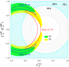
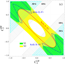
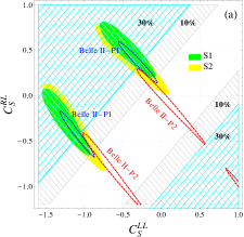
To further discussion, we plot in Fig. 1 the 95% confidence level (C.L.) allowed parameter space in the planes: (a) (CSLL,CSRLsuperscriptsubscript𝐶𝑆𝐿𝐿superscriptsubscript𝐶𝑆𝑅𝐿C_{S}^{LL},C_{S}^{RL}), (b) (CSLL,CSLRsuperscriptsubscript𝐶𝑆𝐿𝐿superscriptsubscript𝐶𝑆𝐿𝑅C_{S}^{LL},C_{S}^{LR}) or (CSLL,CSRRsuperscriptsubscript𝐶𝑆𝐿𝐿superscriptsubscript𝐶𝑆𝑅𝑅C_{S}^{LL},C_{S}^{RR}), and (c) (CSLR,CSRRsuperscriptsubscript𝐶𝑆𝐿𝑅superscriptsubscript𝐶𝑆𝑅𝑅C_{S}^{LR},C_{S}^{RR}). The green and yellow regions are obtained by considering the set of observables S1 and S2, respectively. The cyan (gray) hatched region shows the disallowed parameter space by BR(Bcτν¯τ)<30%BRsuperscriptsubscript𝐵𝑐superscript𝜏subscript¯𝜈𝜏percent30{\rm BR}(B_{c}^{-}\to\tau^{-}\bar{\nu}_{\tau})<30\% (10%percent1010\%). The projections Belle II-P1 and Belle II-P2 for an integrated luminosity of 50ab150superscriptab150\ {\rm ab}^{-1} are illustrated by the blue dotted and red dashed contour lines, respectively. In all of the two WCs scenarios considered, the allowed regions by the set of observables S1 (dominated by R(D())𝑅superscript𝐷R(D^{(\ast)}) HFLAV) are ruled out by BR(Bcτν¯τ)<30%BRsuperscriptsubscript𝐵𝑐superscript𝜏subscript¯𝜈𝜏percent30{\rm BR}(B_{c}^{-}\to\tau^{-}\bar{\nu}_{\tau})<30\% and 10%percent1010\%. This is in agreement with recent analyses Murgui:2019czp ; Mandal:2020htr ; Shi:2019gxi ; Blanke:2018yud ; Blanke:2019qrx . On the contrary, it is observed that there are small allowed regions by the set of observables S2 without violating BR(Bcτν¯τ)<30%BRsuperscriptsubscript𝐵𝑐superscript𝜏subscript¯𝜈𝜏percent30{\rm BR}(B_{c}^{-}\to\tau^{-}\bar{\nu}_{\tau})<30\% and 10%percent1010\%. On the other hand, regarding the Belle II experiment, the available regions from projection Belle II-P1 indicate that these WCs scenarios would be excluded. In contrast, the projection Belle II-P2 would provide stronger constraints than BR(Bcτν¯τ)<30%BRsuperscriptsubscript𝐵𝑐superscript𝜏subscript¯𝜈𝜏percent30{\rm BR}(B_{c}^{-}\to\tau^{-}\bar{\nu}_{\tau})<30\% and 10%percent1010\%, but still allowing a small window for NP contributions. Let us notice that projection Belle II-P2 would cover a similar region to the one set from the analysis of the mono-tau signature ppτhX+MET𝑝𝑝subscript𝜏𝑋METpp\to\tau_{h}X+\rm{MET} at the LHC, as well as the projected sensitivity at the high-luminosity LHC Shi:2019gxi .
Refer to caption
Refer to caption
Refer to caption
Figure 1: The 95% C.L. allowed parameter space for the set of observables S1 [green region] and S2 [yellow region] in the planes: (a) (CSLL,CSRLsuperscriptsubscript𝐶𝑆𝐿𝐿superscriptsubscript𝐶𝑆𝑅𝐿C_{S}^{LL},C_{S}^{RL}), (b) (CSLL,CSLRsuperscriptsubscript𝐶𝑆𝐿𝐿superscriptsubscript𝐶𝑆𝐿𝑅C_{S}^{LL},C_{S}^{LR}) or (CSLL,CSRRsuperscriptsubscript𝐶𝑆𝐿𝐿superscriptsubscript𝐶𝑆𝑅𝑅C_{S}^{LL},C_{S}^{RR}), and (c) (CSLR,CSRRsuperscriptsubscript𝐶𝑆𝐿𝑅superscriptsubscript𝐶𝑆𝑅𝑅C_{S}^{LR},C_{S}^{RR}). The cyan and gray hatched regions represent the excluded regions by the 30% and 10% upper limits on BR(Bcτν¯τ)BRsubscript𝐵𝑐𝜏subscript¯𝜈𝜏{\rm BR}(B_{c}\to\tau\bar{\nu}_{\tau}), respectively. The projections Belle II-P1 and Belle II-P2 for an integrated luminosity of 50ab150superscriptab150\ {\rm ab}^{-1} are illustrated by the blue dotted and red dashed contour lines, respectively (See the text for details).

III.5 Analysis on the parametric space of Yukawa couplings

In this section we are going to discuss the main purpose of this work. We explore the implications on the parametric space associated with the charged Higgs Yukawa couplings to the quarks and leptons in the generic 2HDM that can accomodate the charged-current B𝐵B meson anomalies. In the literature, 2HDMs with a more generic flavor structure have been extensively explored as an explanation to the R(D())𝑅superscript𝐷R(D^{(\ast)}) discrepancies Crivellin:2012ye ; Crivellin:2013wna ; Celis:2012dk ; Celis:2016azn ; Ko:2012sv ; HernandezSanchez:2012eg ; Crivellin:2015hha ; Cline:2015lqp ; Enomoto:2015wbn ; Dhargyal:2016eri ; Martinez:2018ynq ; Wang:2016ggf ; Chen:2017eby ; Iguro:2018fni ; Iguro:2017ysu ; Arbey:2017gmh ; Chen:2018hqy ; Hagiwara:2014tsa ; Lee:2017kbi . In all these works, the neutrinos have been considered to be LH. Only in Refs. Cline:2015lqp ; Iguro:2018qzf ; Li:2018rax , a generic 2HDM involving RH neutrinos has been studied to address the anomalies. Most of these models were implemented by considering the 2018 HFLAV averages and, in addition, none of them include the experimental measurements of polarizations of the Dsuperscript𝐷D^{*} meson and the τ𝜏\tau lepton, the R(J/ψ)𝑅𝐽𝜓R(J/\psi) observable, the latest Belle results and the projected measurements at the ongoing Belle II experiment. In the following analysis all these ingredients are taken into account.

We study the scenarios for a charged scalar boson with general Yukawa couplings involving LH and RH neutrinos. By “general” we will refer to Yukawa couplings without additional assumptions, such as Cheng-Sher ansatz (see, for instance Wang:2016ggf ; Chen:2017eby ). In order to provide an explanation to the bcτν¯τ𝑏𝑐𝜏subscript¯𝜈𝜏b\to c\tau\bar{\nu}_{\tau} anomalies, we will adopt the phenomenological assumption in which the charged scalar boson (H±superscript𝐻plus-or-minusH^{\pm}) couples only to the bottom-charm quarks and the third generation of leptons τ𝜏\tau-ντsubscript𝜈𝜏\nu_{\tau}, i.e., the corresponding Yukawa couplings are differente from zero, while the other ones are taken to be zero. Therefore, NP effects are negligible for light lepton modes (e𝑒e or μ𝜇\mu). In addition, we consider these Yukawa couplings as real (charge-parity conserving) arbitrary free parameters.

The most general Lagrangian for the bcτν¯τ𝑏𝑐𝜏subscript¯𝜈𝜏b\rightarrow c\tau\bar{\nu}_{\tau} transition induced by the Yukawa couplings of a charged scalar boson H±superscript𝐻plus-or-minusH^{\pm} is given by (see Eq. (A))

H±(bcτν¯τ)=subscriptsuperscript𝐻plus-or-minus𝑏𝑐𝜏subscript¯𝜈𝜏absent\displaystyle\mathcal{L}_{H^{\pm}}(b\rightarrow c\tau\bar{\nu}_{\tau})= H+(c¯XcbDPRbc¯XbcUPLb+ν¯τXνττEPRτν¯τXτντNPLτ)superscript𝐻¯𝑐subscriptsuperscript𝑋𝐷𝑐𝑏subscript𝑃𝑅𝑏¯𝑐subscriptsuperscript𝑋𝑈𝑏𝑐subscript𝑃𝐿𝑏subscript¯𝜈𝜏subscriptsuperscript𝑋𝐸subscript𝜈𝜏𝜏subscript𝑃𝑅𝜏subscript¯𝜈𝜏subscriptsuperscript𝑋𝑁𝜏subscript𝜈𝜏subscript𝑃𝐿𝜏\displaystyle-H^{+}\left(\bar{c}X^{D}_{cb}P_{R}b-\bar{c}X^{U*}_{bc}P_{L}b+\bar{\nu}_{\tau}X^{E}_{\nu_{\tau}\tau}P_{R}\tau-\bar{\nu}_{\tau}X^{N*}_{\tau\nu_{\tau}}P_{L}\tau\right)
H(b¯XcbDPLcb¯XbcUPRc+τ¯XνττEPLνττ¯XτντNPRντ),superscript𝐻¯𝑏subscriptsuperscript𝑋𝐷𝑐𝑏subscript𝑃𝐿𝑐¯𝑏subscriptsuperscript𝑋𝑈𝑏𝑐subscript𝑃𝑅𝑐¯𝜏subscriptsuperscript𝑋𝐸subscript𝜈𝜏𝜏subscript𝑃𝐿subscript𝜈𝜏¯𝜏subscriptsuperscript𝑋𝑁𝜏subscript𝜈𝜏subscript𝑃𝑅subscript𝜈𝜏\displaystyle-H^{-}\left(\bar{b}X^{D*}_{cb}P_{L}c-\bar{b}X^{U}_{bc}P_{R}c+\bar{\tau}X^{E*}_{\nu_{\tau}\tau}P_{L}\nu_{\tau}-\bar{\tau}X^{N}_{\tau\nu_{\tau}}P_{R}\nu_{\tau}\right), (10)

where XbcUsubscriptsuperscript𝑋𝑈𝑏𝑐X^{U}_{bc}, XcbDsubscriptsuperscript𝑋𝐷𝑐𝑏X^{D}_{cb}, XνττEsubscriptsuperscript𝑋𝐸subscript𝜈𝜏𝜏X^{E}_{\nu_{\tau}\tau}, and XτντNsubscriptsuperscript𝑋𝑁𝜏subscript𝜈𝜏X^{N}_{\tau\nu_{\tau}} are the Yukawa couplings to the up-quarks, down-quarks, charged leptons and neutrinos, respectively, with Xghf=(Xhgf)superscriptsubscript𝑋𝑔𝑓superscriptsuperscriptsubscript𝑋𝑔𝑓X_{gh}^{f}=(X_{hg}^{f})^{*}. We will use the shorthand notation XτEXνττEsubscriptsuperscript𝑋𝐸𝜏subscriptsuperscript𝑋𝐸subscript𝜈𝜏𝜏X^{E}_{\tau}\equiv X^{E}_{\nu_{\tau}\tau} and XτNXτντNsubscriptsuperscript𝑋𝑁𝜏subscriptsuperscript𝑋𝑁𝜏subscript𝜈𝜏X^{N}_{\tau}\equiv X^{N}_{\tau\nu_{\tau}}. In particular, we want to emphasize that the fourth and eighth terms in the previous expression correspond to the neutrino Yukawa coupling XτNsubscriptsuperscript𝑋𝑁𝜏X^{N}_{\tau}, which describes the interaction between the RH neutrino and a charged scalar boson. While the third and sixth terms correspond to the charged lepton (electron-like) Yukawa coupling XτEsubscriptsuperscript𝑋𝐸𝜏X^{E}_{\tau} that usually appears for LH neutrinos. In Appendix A, we provide details on the derivation of the Yukawa Lagrangian, Eq. (III.5), within a general 2HDM with the inclusion of RH neutrinos. To avoid dangerous tree-level flavor-changing neutral currents, we will impose the aligned condition on the down-type quarks Li:2018rax .

After integrating out H±superscript𝐻plus-or-minusH^{\pm}, the scalar WCs from the effective four-fermion Lagrangian, Eq. (1), are written as (see appendix A.1)

CSLLsubscriptsuperscript𝐶𝐿𝐿𝑆\displaystyle C^{LL}_{S} =\displaystyle= +24GFVcbCKM(XbcU)(XτE)MH±2,24subscript𝐺𝐹subscriptsuperscript𝑉CKM𝑐𝑏subscriptsuperscript𝑋𝑈𝑏𝑐subscriptsuperscript𝑋𝐸𝜏superscriptsubscript𝑀superscript𝐻plus-or-minus2\displaystyle+\frac{\sqrt{2}}{4G_{F}V^{\rm CKM}_{cb}}\frac{\left(X^{U*}_{bc}\right)\left(X^{E*}_{\tau}\right)}{M_{H^{\pm}}^{2}}, (11)
CSRLsubscriptsuperscript𝐶𝑅𝐿𝑆\displaystyle C^{RL}_{S} =\displaystyle= 24GFVcbCKM(XcbD)(XτE)MH±2,24subscript𝐺𝐹subscriptsuperscript𝑉CKM𝑐𝑏subscriptsuperscript𝑋𝐷𝑐𝑏subscriptsuperscript𝑋𝐸𝜏superscriptsubscript𝑀superscript𝐻plus-or-minus2\displaystyle-\frac{\sqrt{2}}{4G_{F}V^{\rm CKM}_{cb}}\frac{\left(X^{D}_{cb}\right)\left(X^{E*}_{\tau}\right)}{M_{H^{\pm}}^{2}}, (12)
CSLRsubscriptsuperscript𝐶𝐿𝑅𝑆\displaystyle C^{LR}_{S} =\displaystyle= 24GFVcbCKM(XbcU)(XτN)MH±2,24subscript𝐺𝐹subscriptsuperscript𝑉CKM𝑐𝑏subscriptsuperscript𝑋𝑈𝑏𝑐subscriptsuperscript𝑋𝑁𝜏superscriptsubscript𝑀superscript𝐻plus-or-minus2\displaystyle-\frac{\sqrt{2}}{4G_{F}V^{\rm CKM}_{cb}}\frac{\left(X^{U*}_{bc}\right)\left(X^{N}_{\tau}\right)}{M_{H^{\pm}}^{2}}, (13)
CSRRsubscriptsuperscript𝐶𝑅𝑅𝑆\displaystyle C^{RR}_{S} =\displaystyle= +24GFVcbCKM(XcbD)(XτN)MH±2,24subscript𝐺𝐹subscriptsuperscript𝑉CKM𝑐𝑏subscriptsuperscript𝑋𝐷𝑐𝑏subscriptsuperscript𝑋𝑁𝜏superscriptsubscript𝑀superscript𝐻plus-or-minus2\displaystyle+\frac{\sqrt{2}}{4G_{F}V^{\rm CKM}_{cb}}\frac{\left(X^{D}_{cb}\right)\left(X^{N}_{\tau}\right)}{M_{H^{\pm}}^{2}}, (14)

with MH±subscript𝑀superscript𝐻plus-or-minusM_{H^{\pm}} being the H±superscript𝐻plus-or-minusH^{\pm} charged scalar boson mass. Thus, the bcτν¯τ𝑏𝑐𝜏subscript¯𝜈𝜏b\rightarrow c\tau\bar{\nu}_{\tau} observables, Eqs. (2) to (8), can be expressed in terms of the effective scalar and pseudoscalar contributions, namely

CSRL±CSLLplus-or-minussubscriptsuperscript𝐶𝑅𝐿𝑆subscriptsuperscript𝐶𝐿𝐿𝑆\displaystyle C^{RL}_{S}\pm C^{LL}_{S} =\displaystyle= 24GFVcbCKM(±XbcUXcbD)(XτE)MH±2,24subscript𝐺𝐹subscriptsuperscript𝑉CKM𝑐𝑏plus-or-minussubscriptsuperscript𝑋𝑈𝑏𝑐subscriptsuperscript𝑋𝐷𝑐𝑏subscriptsuperscript𝑋𝐸𝜏superscriptsubscript𝑀superscript𝐻plus-or-minus2\displaystyle\frac{\sqrt{2}}{4G_{F}V^{\rm CKM}_{cb}}\frac{\left(\pm X^{U*}_{bc}-X^{D}_{cb}\right)\left(X^{E*}_{\tau}\right)}{M_{H^{\pm}}^{2}}, (15)
CSLR±CSRRplus-or-minussubscriptsuperscript𝐶𝐿𝑅𝑆subscriptsuperscript𝐶𝑅𝑅𝑆\displaystyle C^{LR}_{S}\pm C^{RR}_{S} =\displaystyle= 24GFVcbCKM(XbcU±XcbD)(XτN)MH±2,24subscript𝐺𝐹subscriptsuperscript𝑉CKM𝑐𝑏plus-or-minussubscriptsuperscript𝑋𝑈𝑏𝑐subscriptsuperscript𝑋𝐷𝑐𝑏subscriptsuperscript𝑋𝑁𝜏superscriptsubscript𝑀superscript𝐻plus-or-minus2\displaystyle\frac{\sqrt{2}}{4G_{F}V^{\rm CKM}_{cb}}\frac{\left(-X^{U*}_{bc}\pm X^{D}_{cb}\right)\left(X^{N}_{\tau}\right)}{M_{H^{\pm}}^{2}}, (16)

for LH and RH neutrinos, respectively. In the most general case, three Yukawa couplings are always involved in a non trivial way. Keeping this in mind, we perform a χ2superscript𝜒2\chi^{2} analysis by allowing three Yukawa couplings different from zero, i.e., (XbcU,XcbD,XτE)subscriptsuperscript𝑋𝑈𝑏𝑐subscriptsuperscript𝑋𝐷𝑐𝑏subscriptsuperscript𝑋𝐸𝜏(X^{U}_{bc},X^{D}_{cb},X^{E}_{\tau}) for LH neutrinos scenarios and (XbcU,XcbD,XτN)subscriptsuperscript𝑋𝑈𝑏𝑐subscriptsuperscript𝑋𝐷𝑐𝑏subscriptsuperscript𝑋𝑁𝜏(X^{U}_{bc},X^{D}_{cb},X^{N}_{\tau}) for RH neutrinos scenarios, respectively. We found that simplified scenarios regarding two Yukawa couplings (up- or down-quark and lepton or neutrino) cannot simultaneously accomodate the R(D)𝑅𝐷R(D) and R(D)𝑅superscript𝐷R(D^{\ast}) data (even relaxing the uncertainties at the 2σ2𝜎2\sigma level) yielding to p𝑝p-values 8%less-than-or-similar-toabsentpercent8\lesssim 8\%.

Set S1 (χSM2=19.1superscriptsubscript𝜒SM219.1\chi_{\rm SM}^{2}=19.1, p𝑝p-value=SM7.6×104{}_{\rm SM}=7.6\times 10^{-4})
Yukawa couplings BFP p𝑝p-value (%) pullSMsubscriptpullSM\rm{pull_{SM}}
(XbcU,XcbD,XτE)subscriptsuperscript𝑋𝑈𝑏𝑐subscriptsuperscript𝑋𝐷𝑐𝑏subscriptsuperscript𝑋𝐸𝜏(X^{U}_{bc},X^{D}_{cb},X^{E}_{\tau}) (0.33,0.38,0.47)0.330.380.47(0.33,0.38,-0.47) 28.8 2.95
(XbcU,XcbD,XτN)subscriptsuperscript𝑋𝑈𝑏𝑐subscriptsuperscript𝑋𝐷𝑐𝑏subscriptsuperscript𝑋𝑁𝜏(X^{U}_{bc},X^{D}_{cb},X^{N}_{\tau}) (0.35,0.25,1.09)0.350.251.09(-0.35,-0.25,-1.09) 28.9 2.95
Set S2 (χSM2=11.2superscriptsubscript𝜒SM211.2\chi_{\rm SM}^{2}=11.2, p𝑝p-value=SM2.4×102{}_{\rm SM}=2.4\times 10^{-2})
Yukawa couplings BFP p𝑝p-value (%) pullSMsubscriptpullSM\rm{pull_{SM}}
(XbcU,XcbD,XτE)subscriptsuperscript𝑋𝑈𝑏𝑐subscriptsuperscript𝑋𝐷𝑐𝑏subscriptsuperscript𝑋𝐸𝜏(X^{U}_{bc},X^{D}_{cb},X^{E}_{\tau}) (0.23,0.25,0.64)0.230.250.64(0.23,0.25,-0.64) 28.4 1.56
(XbcU,XcbD,XτN)subscriptsuperscript𝑋𝑈𝑏𝑐subscriptsuperscript𝑋𝐷𝑐𝑏subscriptsuperscript𝑋𝑁𝜏(X^{U}_{bc},X^{D}_{cb},X^{N}_{\tau}) (0.38,0.31,0.90)0.380.310.90(-0.38,0.31,-0.90) 27.7 1.54
Table 4: BFP values, p𝑝p-value, and pullSMsubscriptpullSM\rm{pull_{SM}} by allowing three Yukawa couplings different from zero to fit the set of observables S1 and S2.

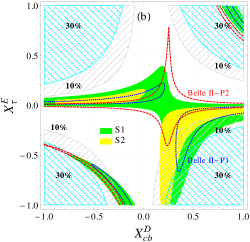
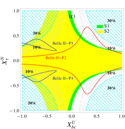
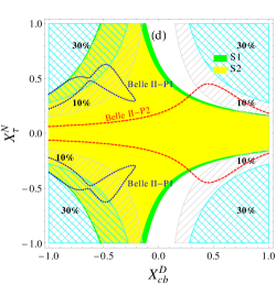
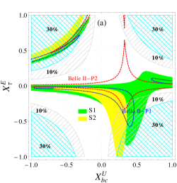
We display in Table 4 the BFP values, p𝑝p-value, and pullSMsubscriptpullSM\rm{pull_{SM}} by allowing three Yukawa couplings different from zero to fit the set of observables S1 and S2. Particularly, we observe that the neutrino Yukawa couplings must be as large as one (|XτN|1similar-tosubscriptsuperscript𝑋𝑁𝜏1|X^{N}_{\tau}|\sim 1) to reproduce the bcτν¯τ𝑏𝑐𝜏subscript¯𝜈𝜏b\rightarrow c\tau\bar{\nu}_{\tau} data. Furthermore, the 95% C.L. allowed two dimensional parameter space in the Yukawa couplings planes: (a) (XbcU,XτEsubscriptsuperscript𝑋𝑈𝑏𝑐subscriptsuperscript𝑋𝐸𝜏X^{U}_{bc},X^{E}_{\tau}), (b) (XcbD,XτEsubscriptsuperscript𝑋𝐷𝑐𝑏subscriptsuperscript𝑋𝐸𝜏X^{D}_{cb},X^{E}_{\tau}), (c) (XbcU,XτNsubscriptsuperscript𝑋𝑈𝑏𝑐subscriptsuperscript𝑋𝑁𝜏X^{U}_{bc},X^{N}_{\tau}) and (d) (XcbD,XτNsubscriptsuperscript𝑋𝐷𝑐𝑏subscriptsuperscript𝑋𝑁𝜏X^{D}_{cb},X^{N}_{\tau}), are shown in Fig. 2. The green and yellow regions represent the allowed parameter space that simultaneously can accommodate the set of observables S1 and S2, respectively. These plots have been obtained for a representative charged Higgs mass of MH±=500subscript𝑀superscript𝐻plus-or-minus500M_{H^{\pm}}=500 GeV, which corresponds to a benchmark mass value usually considered in the literature Chen:2017eby ; Iguro:2017ysu ; Li:2018rax . In each case, we vary the Yukawa couplings on the plane while keeping the remaining one at the BFP. The hatched regions in gray and cyan refer to the excluded regions by the 10% and 30% upper limits on BR(Bcτν¯τ)BRsubscript𝐵𝑐𝜏subscript¯𝜈𝜏{\rm BR}(B_{c}\to\tau\bar{\nu}_{\tau}), respectively. The prospects Belle II-P1 and Belle II-P2 for an integrated luminosity of 50ab150superscriptab150\ {\rm ab}^{-1} Kou:2018nap are illustrated by the blue dotted and red dashed contour lines, respectively. According to our analysis, we get the following remarks:

  1. 1.

    For the Yukawa couplings planes (XbcU,XτEsubscriptsuperscript𝑋𝑈𝑏𝑐subscriptsuperscript𝑋𝐸𝜏X^{U}_{bc},X^{E}_{\tau}) and (XcbD,XτEsubscriptsuperscript𝑋𝐷𝑐𝑏subscriptsuperscript𝑋𝐸𝜏X^{D}_{cb},X^{E}_{\tau}) related with LH neutrinos, panels 2(a) and 2(b), Yukawa couplings regions with absolute values of the order 𝒪(101)𝒪superscript101\mathcal{O}(10^{-1}) are allowed by the set of observables S1 and S2, as well as by the prospects Belle II-P1 and Belle II-P2.

  2. 2.

    As concerns with the neutrino Yukawa couplings planes (XbcU,XτNsubscriptsuperscript𝑋𝑈𝑏𝑐subscriptsuperscript𝑋𝑁𝜏X^{U}_{bc},X^{N}_{\tau}) and (XcbD,XτNsubscriptsuperscript𝑋𝐷𝑐𝑏subscriptsuperscript𝑋𝑁𝜏X^{D}_{cb},X^{N}_{\tau}) (RH neutrino solutions), panels 2(c) and 2(d), both for set of observables S1 and S2 there is a wide allowed region Yukawa couplings with absolute values of the order 𝒪(101)𝒪superscript101\mathcal{O}(10^{-1}), that would be reduced by the projection Belle II-P2. The case of projection Belle II-P1 would be almost excluded because of bounds BR(Bcτν¯τ)<30%BRsuperscriptsubscript𝐵𝑐superscript𝜏subscript¯𝜈𝜏percent30{\rm BR}(B_{c}^{-}\to\tau^{-}\bar{\nu}_{\tau})<30\% and 10%percent1010\%. Our results imply that current experimental bcτν¯τ𝑏𝑐𝜏subscript¯𝜈𝜏b\rightarrow c\tau\bar{\nu}_{\tau} data favors the interpretation of a charged scalar boson with right-handed neutrinos.
Refer to caption
Refer to caption
Refer to caption
Refer to caption
Figure 2: The 95% C.L. allowed two dimensional parameter space for the sets S1 [green region] and S2 [yellow region] in the Yukawa coupling planes: (a) (XbcU,XτEsubscriptsuperscript𝑋𝑈𝑏𝑐subscriptsuperscript𝑋𝐸𝜏X^{U}_{bc},X^{E}_{\tau}), (b) (XbcU,XτNsubscriptsuperscript𝑋𝑈𝑏𝑐subscriptsuperscript𝑋𝑁𝜏X^{U}_{bc},X^{N}_{\tau}), (c) (XcbD,XτEsubscriptsuperscript𝑋𝐷𝑐𝑏subscriptsuperscript𝑋𝐸𝜏X^{D}_{cb},X^{E}_{\tau}) and (d) (XcbD,XτNsubscriptsuperscript𝑋𝐷𝑐𝑏subscriptsuperscript𝑋𝑁𝜏X^{D}_{cb},X^{N}_{\tau}), for a charged Higgs mass of MH±=500subscript𝑀superscript𝐻plus-or-minus500M_{H^{\pm}}=500 GeV. The hatched regions in gray and cyan represent the excluded regions by the 10% and 30% upper limits on BR(Bcτν¯τ)BRsubscript𝐵𝑐𝜏subscript¯𝜈𝜏{\rm BR}(B_{c}\to\tau\bar{\nu}_{\tau}), respectively. The projections Belle II-P1 and Belle II-P2 for an integrated luminosity of 50ab150superscriptab150\ {\rm ab}^{-1} Kou:2018nap are illustrated by the blue dotted and red dashed contour lines, respectively. In each case, we vary the Yukawa couplings on the plane while keeping the remaining one at the BFP.

IV Digging into the relation between R(D)𝑅superscript𝐷R(D^{\ast}) and BR(Bcτν¯τ)BRsuperscriptsubscript𝐵𝑐superscript𝜏subscript¯𝜈𝜏{\rm BR}(B_{c}^{-}\to\tau^{-}\bar{\nu}_{\tau})

The importance of the relation between R(D)𝑅superscript𝐷R(D^{\ast}) and BR(Bcτν¯τ)BRsuperscriptsubscript𝐵𝑐superscript𝜏subscript¯𝜈𝜏{\rm BR}(B_{c}^{-}\to\tau^{-}\bar{\nu}_{\tau}) was first pointed out in Ref. Alonso:2016oyd , where an upper limit of BR(Bcτν¯τ)30%BRsuperscriptsubscript𝐵𝑐superscript𝜏subscript¯𝜈𝜏percent30{\rm BR}(B_{c}^{-}\to\tau^{-}\bar{\nu}_{\tau})\leq 30\% is imposed by considering the lifetime of Bcsubscript𝐵𝑐B_{c} meson. This bound puts strong constraints on the pseudoscalar interpretation to R(D)𝑅superscript𝐷R(D^{\ast}) generated by the effective coupling ϵP=CSRLCSLLsubscriptitalic-ϵ𝑃superscriptsubscript𝐶𝑆𝑅𝐿superscriptsubscript𝐶𝑆𝐿𝐿\epsilon_{P}=C_{S}^{RL}-C_{S}^{LL} Alonso:2016oyd . Later on, a stronger bound of BR(Bcτν¯τ)10%BRsuperscriptsubscript𝐵𝑐superscript𝜏subscript¯𝜈𝜏percent10{\rm BR}(B_{c}^{-}\to\tau^{-}\bar{\nu}_{\tau})\leq 10\% was obtained in Ref. Akeroyd:2017mhr from the LEP data taken at the Z𝑍Z peak. Recently, these limits have been critically examined and relaxed bounds of 39%absentpercent39\leq 39\% Bardhan:2019ljo and 60%absentpercent60\leq 60\% Blanke:2018yud ; Blanke:2019qrx have been obtained. In the following, for completeness, we revisit whether the claim that pseudoscalar NP interpretations of R(D)𝑅superscript𝐷R(D^{\ast}) are implausible Alonso:2016oyd is still valid (or not) to the light of the recent measurements,

R(D)𝑅superscript𝐷\displaystyle R(D^{\ast}) =\displaystyle= 0.295±0.014HFLAV Amhis:2019ckw ; HFLAVsummer ,plus-or-minus0.2950.014HFLAV Amhis:2019ckw ; HFLAVsummer \displaystyle 0.295\pm 0.014\ \ \text{HFLAV~{}\cite[cite]{\@@bibref{Authors Phrase1YearPhrase2}{Amhis:2019ckw,HFLAVsummer}{\@@citephrase{(}}{\@@citephrase{)}}}},
R(D)𝑅superscript𝐷\displaystyle R(D^{\ast}) =\displaystyle= 0.284±0.018Belle combination Belle:2019rba ,plus-or-minus0.2840.018Belle combination Belle:2019rba \displaystyle 0.284\pm 0.018\ \ \text{Belle combination~{}\cite[cite]{\@@bibref{Authors Phrase1YearPhrase2}{Belle:2019rba}{\@@citephrase{(}}{\@@citephrase{)}}}}, (17)
R(D)𝑅superscript𝐷\displaystyle R(D^{\ast}) =\displaystyle= 0.291±0.035LHCb Aaij:2017deq ,plus-or-minus0.2910.035LHCb Aaij:2017deq \displaystyle 0.291\pm 0.035\ \ \text{LHCb~{}\cite[cite]{\@@bibref{Authors Phrase1YearPhrase2}{Aaij:2017deq}{\@@citephrase{(}}{\@@citephrase{)}}}},

by considering BR(Bcτν¯τ)<30%BRsuperscriptsubscript𝐵𝑐superscript𝜏subscript¯𝜈𝜏percent30{\rm BR}(B_{c}^{-}\to\tau^{-}\bar{\nu}_{\tau})<30\% Alonso:2016oyd and 10%percent1010\% Akeroyd:2017mhr . We also include in our analysis the Belle II prospects Belle II-P1 and Belle II-P2 described in Sec. III, to see the future implications that could be achieved at Belle II for an integrated luminosity of 50 ab1superscriptab1\rm ab^{-1} Kou:2018nap .

Refer to caption
Refer to caption
Refer to caption
Refer to caption
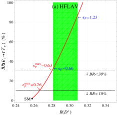
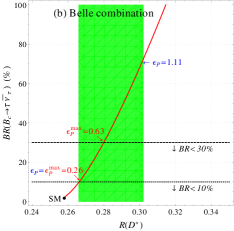
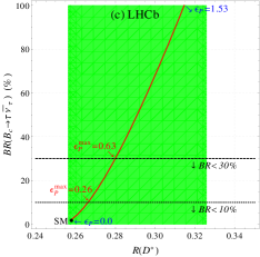
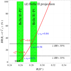
Figure 3: Relation between R(D)𝑅superscript𝐷R(D^{\ast}) and BR(Bcτν¯τ)BRsuperscriptsubscript𝐵𝑐superscript𝜏subscript¯𝜈𝜏{\rm BR}(B_{c}^{-}\to\tau^{-}\bar{\nu}_{\tau}) for R(D)𝑅superscript𝐷R(D^{\ast}) from (a) HFLAV Amhis:2019ckw ; HFLAVsummer , (b) Belle combination Belle:2019rba , (c) LHCb Aaij:2017deq , and (d) Belle II prospects Belle II-P1 and Belle II-P2; represented by the green 1σ1𝜎1\sigma band, respectively. The red solid line shows the parametric dependence of R(D)𝑅superscript𝐷R(D^{\ast}) and BR(Bcτν¯τ)BRsuperscriptsubscript𝐵𝑐superscript𝜏subscript¯𝜈𝜏{\rm BR}(B_{c}^{-}\to\tau^{-}\bar{\nu}_{\tau}) on the effective coupling ϵPsubscriptitalic-ϵ𝑃\epsilon_{P}. The dashed (dotted) horizontal line represents BR(Bcτν¯τ)<30%BRsuperscriptsubscript𝐵𝑐superscript𝜏subscript¯𝜈𝜏percent30{\rm BR}(B_{c}^{-}\to\tau^{-}\bar{\nu}_{\tau})<30\% (10%percent1010\%).

In Fig. 3 we plot the relation between R(D)𝑅superscript𝐷R(D^{\ast}) and BR(Bcτν¯τ)BRsuperscriptsubscript𝐵𝑐superscript𝜏subscript¯𝜈𝜏{\rm BR}(B_{c}^{-}\to\tau^{-}\bar{\nu}_{\tau}) for R(D)𝑅superscript𝐷R(D^{\ast}) from (a) HFLAV Amhis:2019ckw ; HFLAVsummer , (b) Belle combination Belle:2019rba , (c) LHCb Aaij:2017deq , and (d) Belle II prospects Belle II-P1 and Belle II-P1 for 50 ab1superscriptab1\rm ab^{-1}. In all the cases, the band represents the 1σ1𝜎1\sigma experimental value. The red solid line shows the parametric dependence of R(D)𝑅superscript𝐷R(D^{\ast}) and BR(Bcτν¯τ)BRsuperscriptsubscript𝐵𝑐superscript𝜏subscript¯𝜈𝜏{\rm BR}(B_{c}^{-}\to\tau^{-}\bar{\nu}_{\tau}) on the effective coupling ϵPsubscriptitalic-ϵ𝑃\epsilon_{P}, while the dashed and dotted horizontal lines represent the upper limit BR(Bcτν¯τ)<30%BRsuperscriptsubscript𝐵𝑐superscript𝜏subscript¯𝜈𝜏percent30{\rm BR}(B_{c}^{-}\to\tau^{-}\bar{\nu}_{\tau})<30\% and 10%percent1010\%, respectively. The SM value is represented by the black circle. It is found that the 1σ1𝜎1\sigma allowed solutions are

HFLAVHFLAV\displaystyle{\rm HFLAV} ::\displaystyle: ϵP=[0.66,1.23],subscriptitalic-ϵ𝑃0.661.23\displaystyle\ \epsilon_{P}=[0.66,1.23],
BellecombinationBellecombination\displaystyle{\rm Belle\ combination} ::\displaystyle: ϵP=[0.26,1.11],subscriptitalic-ϵ𝑃0.261.11\displaystyle\ \epsilon_{P}=[0.26,1.11],
LHCbLHCb\displaystyle{\rm LHCb} ::\displaystyle: ϵP=[0.0,1.53],subscriptitalic-ϵ𝑃0.01.53\displaystyle\ \epsilon_{P}=[0.0,1.53], (18)
Belle II-P1 ::\displaystyle: ϵP=[0.58,0.86],subscriptitalic-ϵ𝑃0.580.86\displaystyle\ \epsilon_{P}=[0.58,0.86],
Belle II-P2 ::\displaystyle: ϵP=[0.0,0.23],subscriptitalic-ϵ𝑃0.00.23\displaystyle\ \epsilon_{P}=[0.0,0.23],

respectively, as depicted in Fig. 3. In order to fulfill the bound BR(Bcτν¯τ)<30%BRsuperscriptsubscript𝐵𝑐superscript𝜏subscript¯𝜈𝜏percent30{\rm BR}(B_{c}^{-}\to\tau^{-}\bar{\nu}_{\tau})<30\% (10%)10\%), the maximum value required is ϵPmax=0.63subscriptsuperscriptitalic-ϵmax𝑃0.63\epsilon^{\rm max}_{P}=0.63 (0.260.260.26), corresponding to a value of R(D)=0.281𝑅superscript𝐷0.281R(D^{\ast})=0.281 (0.2660.2660.266). For the case of HFLAV, the allowed ϵPsubscriptitalic-ϵ𝑃\epsilon_{P} values violate the bound BR(Bcτν¯τ)<30%BRsuperscriptsubscript𝐵𝑐superscript𝜏subscript¯𝜈𝜏percent30{\rm BR}(B_{c}^{-}\to\tau^{-}\bar{\nu}_{\tau})<30\%. In contrast, the allowed ϵPsubscriptitalic-ϵ𝑃\epsilon_{P} values for Belle combination satisfy both BR(Bcτν¯τ)<30%BRsuperscriptsubscript𝐵𝑐superscript𝜏subscript¯𝜈𝜏percent30{\rm BR}(B_{c}^{-}\to\tau^{-}\bar{\nu}_{\tau})<30\% and 10%percent1010\%. On the other hand, the experimental uncertainties of the LHCb data are large enough to be consistent with the bounds BR(Bcτν¯τ)<30%BRsuperscriptsubscript𝐵𝑐superscript𝜏subscript¯𝜈𝜏percent30{\rm BR}(B_{c}^{-}\to\tau^{-}\bar{\nu}_{\tau})<30\% and 10%percent1010\%, as well as with the SM. As for the Belle II-P1 would only respect the limit of 30%percent3030\%, while for Belle II-P2, small values of ϵPsubscriptitalic-ϵ𝑃\epsilon_{P} would be favored in fulfillment with the limits of 30%percent3030\% and 10%percent1010\%. In addition, Belle II-P2 would also be able to prove an aggressive bound of BR(Bcτν¯τ)<5%BRsuperscriptsubscript𝐵𝑐superscript𝜏subscript¯𝜈𝜏percent5{\rm BR}(B_{c}^{-}\to\tau^{-}\bar{\nu}_{\tau})<5\%.

Therefore, BR(Bcτν¯τ)<30%BRsuperscriptsubscript𝐵𝑐superscript𝜏subscript¯𝜈𝜏percent30{\rm BR}(B_{c}^{-}\to\tau^{-}\bar{\nu}_{\tau})<30\% Alonso:2016oyd still disfavors the ϵPsubscriptitalic-ϵ𝑃\epsilon_{P} pseudoscalar explanation of the R(D)𝑅superscript𝐷R(D^{\ast}) HFLAV average, while this is no longer the case for the R(D)𝑅superscript𝐷R(D^{\ast}) data from Belle combination Belle:2019rba and LHCb Aaij:2017deq . The projection Belle II-P1 would not be in conflict with BR(Bcτν¯τ)<30%BRsuperscriptsubscript𝐵𝑐superscript𝜏subscript¯𝜈𝜏percent30{\rm BR}(B_{c}^{-}\to\tau^{-}\bar{\nu}_{\tau})<30\%, whereas the projection Belle II-P2 would lead to stronger constraints than those obtained from BR(Bcτν¯τ)BRsuperscriptsubscript𝐵𝑐superscript𝜏subscript¯𝜈𝜏{\rm BR}(B_{c}^{-}\to\tau^{-}\bar{\nu}_{\tau}). Certainly, future measurements by the Belle II Kou:2018nap (as well as LHCb) experiment are required in order to clarify this situation.
Refer to caption
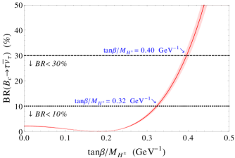
Figure 4: BR(Bcτν¯τ)BRsuperscriptsubscript𝐵𝑐superscript𝜏subscript¯𝜈𝜏{\rm BR}(B_{c}^{-}\to\tau^{-}\bar{\nu}_{\tau}) in the 2HDM of type II as a function of tanβ/MH±𝛽subscript𝑀superscript𝐻plus-or-minus\tan\beta/M_{H^{\pm}} (red solid line). The light-red band represents the 1σ1𝜎1\sigma error, while the dashed and dotted horizontal lines represent BR(Bcτν¯τ)<30%BRsuperscriptsubscript𝐵𝑐superscript𝜏subscript¯𝜈𝜏percent30{\rm BR}(B_{c}^{-}\to\tau^{-}\bar{\nu}_{\tau})<30\% and 10%percent1010\%, respectively.

V Reexamining the explanation from 2HDM of Type II

Although our principal interest is to study the effects of a charged scalar boson Higgs with right-handed neutrinos to the bcτν¯τ𝑏𝑐𝜏subscript¯𝜈𝜏b\to c\tau\bar{\nu}_{\tau} transition, in this section we discuss whether the 2HDM of Type II can still explain the R(D())𝑅superscript𝐷R(D^{(*)}) anomalies in light of current measurements. This analysis is relevant because this model is an important NP scenario in the study of the charged-current B𝐵B anomalies.

The 2HDM of Type II provides one of the simplest scenarios with charged scalar bosons (H±superscript𝐻plus-or-minusH^{\pm}). Within this framework, the NP effects of a charged Higgs boson depend on the mass of charged scalar boson MH±subscript𝑀superscript𝐻plus-or-minusM_{H^{\pm}} and tanβ𝛽\tan\beta (defined as the ratio of vacuum expectation values v2/v1subscript𝑣2subscript𝑣1v_{2}/v_{1}), which are described in terms of a single parameter, tanβ/MH±𝛽subscript𝑀superscript𝐻plus-or-minus\tan\beta/M_{H^{\pm}}. In the 2HDM of Type II, tree-level charged Higgs boson contributions to the B𝐵B meson processes induced by the semileptonic transition bcτν¯τ𝑏𝑐𝜏subscript¯𝜈𝜏b\to c\tau\bar{\nu}_{\tau} have been investigated (See, for instance Hou:1992sy ; Tanaka:1994ay ; Tanaka:2010se ; Kamenik:2008tj ; Nierste:2008qe ; Fajfer:2012vx ). In 2012 and 2013, the BABAR Collaboration with their full data sample reported a disagreement on the measurements of the ratio of semileptonic B𝐵B decays, R(D)𝑅𝐷R(D) and R(D)𝑅superscript𝐷R(D^{\ast}), with respect to the SM predictions Lees:2012xj ; Lees:2013uzd . According to the BABAR results, the 2HDM of Type II cannot explain simultaneously the R(D())𝑅superscript𝐷R(D^{(\ast)}) discrepancies Lees:2012xj ; Lees:2013uzd . Since then (and to date), the 2HDM of Type II interpretation was ruled out and 2HDM models with a more generic flavor structure were considered in the literature Crivellin:2012ye ; Crivellin:2013wna ; Celis:2012dk ; Celis:2016azn ; Ko:2012sv ; HernandezSanchez:2012eg ; Crivellin:2015hha ; Cline:2015lqp ; Enomoto:2015wbn ; Dhargyal:2016eri ; Martinez:2018ynq ; Wang:2016ggf ; Chen:2017eby ; Iguro:2018fni ; Iguro:2017ysu ; Arbey:2017gmh ; Chen:2018hqy ; Hagiwara:2014tsa ; Lee:2017kbi ; Iguro:2018qzf ; Li:2018rax . It is worth noting that subsequent analysis performed by Belle Collaboration in 2015 Huschle:2015rga and 2016 Sato:2016svk showed compatibility with the 2HDM of Type II in the tanβ/MH±𝛽subscript𝑀superscript𝐻plus-or-minus\tan\beta/M_{H^{\pm}} regions around 0.45GeV10.45superscriptGeV10.45\ {\rm GeV}^{-1} Huschle:2015rga and [0.65,0.76]GeV10.650.76superscriptGeV1[0.65,0.76]\ {\rm GeV}^{-1} Sato:2016svk , respectively, in contradiction with the BABAR measurements Lees:2012xj ; Lees:2013uzd . Thereby, given the current experimental situation on the R(D())𝑅superscript𝐷R(D^{(\ast)}) anomalies, HFLAV Amhis:2019ckw ; HFLAVsummer and Belle combination Belle:2019rba , and the Belle II future sensitivity Kou:2018nap , in the following we reexamine whether the 2HDM of Type II is still ruled out (or not) as an explanation to the R(D())𝑅superscript𝐷R(D^{(\ast)}) anomalies. In addition, it is also important to confront this model not only to the R(D())𝑅superscript𝐷R(D^{(\ast)}) measurements but also to all bcτν¯τ𝑏𝑐𝜏subscript¯𝜈𝜏b\to c\tau\bar{\nu}_{\tau} observables.

By construction, in the 2HDM of Type II the neutrinos are considered to be LH, therefore, the scalar WCs that contribute to the charged-current bcτν¯τ𝑏𝑐𝜏subscript¯𝜈𝜏b\to c\tau\bar{\nu}_{\tau} are written as Sato:2016svk ; Tanaka:2010se ; Tanaka:2012nw

CSRLsuperscriptsubscript𝐶𝑆𝑅𝐿\displaystyle C_{S}^{RL} =\displaystyle= mbmτtanβMH±2,subscript𝑚𝑏subscript𝑚𝜏𝛽superscriptsubscript𝑀superscript𝐻plus-or-minus2\displaystyle-\frac{m_{b}m_{\tau}\tan\beta}{M_{H^{\pm}}^{2}}, (19)
CSLLsuperscriptsubscript𝐶𝑆𝐿𝐿\displaystyle C_{S}^{LL} =\displaystyle= mcmτMH±2,subscript𝑚𝑐subscript𝑚𝜏superscriptsubscript𝑀superscript𝐻plus-or-minus2\displaystyle-\frac{m_{c}m_{\tau}}{M_{H^{\pm}}^{2}}, (20)

where mbsubscript𝑚𝑏m_{b}, mcsubscript𝑚𝑐m_{c}, and mτsubscript𝑚𝜏m_{\tau} are the masses of the bottom quark, charm quark, and τ𝜏\tau lepton, respectively. In the literature Sato:2016svk ; Tanaka:2010se ; Tanaka:2012nw , the coefficient CSLLsuperscriptsubscript𝐶𝑆𝐿𝐿C_{S}^{LL} is usually neglected (CSLL0similar-to-or-equalssuperscriptsubscript𝐶𝑆𝐿𝐿0C_{S}^{LL}\simeq 0), thus, the charged Higgs boson effect is only dominated by CSRLsuperscriptsubscript𝐶𝑆𝑅𝐿C_{S}^{RL} which is driven by tanβ/MH±𝛽subscript𝑀superscript𝐻plus-or-minus\tan\beta/M_{H^{\pm}}. We begin our analysis by considering the constraints on the parameter tanβ/MH±𝛽subscript𝑀superscript𝐻plus-or-minus\tan\beta/M_{H^{\pm}} from the upper limits BR(Bcτν¯τ)<30%BRsuperscriptsubscript𝐵𝑐superscript𝜏subscript¯𝜈𝜏percent30{\rm BR}(B_{c}^{-}\to\tau^{-}\bar{\nu}_{\tau})<30\% Alonso:2016oyd and 10%percent1010\% Akeroyd:2017mhr . In Fig. 4 we show the BR(Bcτν¯τ)BRsuperscriptsubscript𝐵𝑐superscript𝜏subscript¯𝜈𝜏{\rm BR}(B_{c}^{-}\to\tau^{-}\bar{\nu}_{\tau}) in the 2HDM of type II as a function of tanβ/MH±𝛽subscript𝑀superscript𝐻plus-or-minus\tan\beta/M_{H^{\pm}} (red solid line), where the dashed and dotted horizontal lines represent BR(Bcτν¯τ)<30%BRsuperscriptsubscript𝐵𝑐superscript𝜏subscript¯𝜈𝜏percent30{\rm BR}(B_{c}^{-}\to\tau^{-}\bar{\nu}_{\tau})<30\% and 10%percent1010\%, respectively. We get the following strong bounds

tanβ/MH±<0.40(0.32),𝛽subscript𝑀superscript𝐻plus-or-minus0.400.32\displaystyle\tan\beta/M_{H^{\pm}}<0.40\ (0.32), (21)

for BR(Bcτν¯τ)<30%BRsuperscriptsubscript𝐵𝑐superscript𝜏subscript¯𝜈𝜏percent30{\rm BR}(B_{c}^{-}\to\tau^{-}\bar{\nu}_{\tau})<30\% (10%percent1010\%), implying that large values of tanβ/MH±𝛽subscript𝑀superscript𝐻plus-or-minus\tan\beta/M_{H^{\pm}} are excluded. This plot has been obtained by using the SM estimation BR(Bcτν¯τ)SM=(2.16±0.16)%BRsubscriptsuperscriptsubscript𝐵𝑐superscript𝜏subscript¯𝜈𝜏SMpercentplus-or-minus2.160.16{\rm BR}(B_{c}^{-}\to\tau^{-}\bar{\nu}_{\tau})_{\rm SM}=(2.16\pm 0.16)\% Gomez:2019xfw . In addition, in Table 5 we present the 2σ2𝜎2\sigma allowed regions by each of the bcτν¯τ𝑏𝑐𝜏subscript¯𝜈𝜏b\to c\tau\bar{\nu}_{\tau} observables on the parameter tanβ/MH±𝛽subscript𝑀superscript𝐻plus-or-minus\tan\beta/M_{H^{\pm}}, namely, R(D())𝑅superscript𝐷R(D^{(\ast)}) HFLAV and Belle combination, R(J/ψ),FL(D),Pτ(D)𝑅𝐽𝜓subscript𝐹𝐿superscript𝐷subscript𝑃𝜏superscript𝐷R(J/\psi),F_{L}(D^{*}),P_{\tau}(D^{*}), and R(Xc)𝑅subscript𝑋𝑐R(X_{c}). Regarding the Belle II future scenario described in Sec. III, we also show the prospects Belle II-P1 and Belle II-P2 that could be achieved at Belle II for an integrated luminosity of 50 ab1superscriptab1\rm ab^{-1} Kou:2018nap . As a result, it is possible to find a common small values region, tanβ/MH±=[0.0,0.32]𝛽subscript𝑀superscript𝐻plus-or-minus0.00.32\tan\beta/M_{H^{\pm}}=[0.0,0.32], without conflicting with the strongest bound imposed by BR(Bcτν¯τ)<10%BRsuperscriptsubscript𝐵𝑐superscript𝜏subscript¯𝜈𝜏percent10{\rm BR}(B_{c}^{-}\to\tau^{-}\bar{\nu}_{\tau})<10\%; with the exception of R(D)𝑅superscript𝐷R(D^{\ast}) HFLAV and R(J/ψ)𝑅𝐽𝜓R(J/\psi) that allows large tanβ/MH±𝛽subscript𝑀superscript𝐻plus-or-minus\tan\beta/M_{H^{\pm}} values, which are in tension with BR(Bcτν¯τ)<30%BRsuperscriptsubscript𝐵𝑐superscript𝜏subscript¯𝜈𝜏percent30{\rm BR}(B_{c}^{-}\to\tau^{-}\bar{\nu}_{\tau})<30\% and 10%percent1010\%. Besides, the projected Belle II-P1 values would be rule out by the bounds of 30%percent3030\% and 10%percent1010\%, while the projection Belle II-P2 would point out to small values of tanβ/MH±𝛽subscript𝑀superscript𝐻plus-or-minus\tan\beta/M_{H^{\pm}}.

Observable Allowed regions (2σ2𝜎2\sigma) on tanβ/MH±𝛽subscript𝑀superscript𝐻plus-or-minus\tan\beta/M_{H^{\pm}} (GeV1superscriptGeV1\rm GeV^{-1})
R(D)𝑅𝐷R(D) HFLAV [0.0,0.08][0.44,0.47]0.00.080.440.47[0.0,0.08]\cup[0.44,0.47]
R(D)𝑅𝐷R(D) Belle combination [0.0,0.11][0.43,0.47]0.00.110.430.47[0.0,0.11]\cup[0.43,0.47]
R(D)𝑅𝐷R(D) Belle II-P1 [0.45,0.46]0.450.46[0.45,0.46]
R(D)𝑅𝐷R(D) Belle II-P2 [0.0,0.06][0.44,0.45]0.00.060.440.45[0.0,0.06]\cup[0.44,0.45]
R(D)𝑅superscript𝐷R(D^{*}) HFLAV [0.64,0.75]0.640.75[0.64,0.75]
R(D)𝑅superscript𝐷R(D^{\ast}) Belle combination [0.0,0.24][0.56,0.75]0.00.240.560.75[0.0,0.24]\cup[0.56,0.75]
R(D)𝑅superscript𝐷R(D^{\ast}) Belle II-P1 [0.67,0.70]0.670.70[0.67,0.70]
R(D)𝑅superscript𝐷R(D^{\ast}) Belle II-P2 [0.0,0.17][0.58,0.63]0.00.170.580.63[0.0,0.17]\cup[0.58,0.63]
R(J/ψ)𝑅𝐽𝜓R(J/\psi) [1.0,1.05]1.01.05[1.0,1.05]
FL(D)subscript𝐹𝐿superscript𝐷F_{L}(D^{\ast}) [0.0,0.09][0.44,0.67]0.00.090.440.67[0.0,0.09]\cup[0.44,0.67]
Pτ(D)subscript𝑃𝜏superscript𝐷P_{\tau}(D^{\ast}) [0.0,0.32][0.56,1.03]0.00.320.561.03[0.0,0.32]\cup[0.56,1.03]
R(Xc)𝑅subscript𝑋𝑐R(X_{c}) [0.0,0.17][0.44,0.72]0.00.170.440.72[0.0,0.17]\cup[0.44,0.72]
Table 5: The 2σ2𝜎2\sigma allowed regions on the parameter tanβ/MH±𝛽subscript𝑀superscript𝐻plus-or-minus\tan\beta/M_{H^{\pm}} of the 2HDM of Type II, obtained for the different bcτν¯τ𝑏𝑐𝜏subscript¯𝜈𝜏b\to c\tau\bar{\nu}_{\tau} observables. The Belle II future projections for an integrated luminosity of 50 ab1superscriptab1\rm ab^{-1} are also included.
Refer to caption
Refer to caption
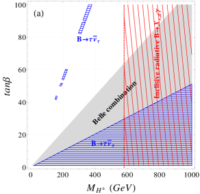
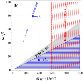
Figure 5: Allowed parameter space in the plane (MH±,tanβ)subscript𝑀superscript𝐻plus-or-minus𝛽(M_{H^{\pm}},\tan\beta) of the 2HDM Type II for (a) Belle combination and (b) Belle II-P2 for 50 ab1superscriptab1\rm ab^{-1}. The allowed regions by Bτν¯τ𝐵𝜏subscript¯𝜈𝜏B\to\tau\bar{\nu}_{\tau} and the inclusive radiative decays BXs,dγ𝐵subscript𝑋𝑠𝑑𝛾B\to X_{s,d}\gamma Misiak:2017bgg are represented by the blue and red hatched regions, respectively.

To further discussion, we now translate these results into the plane (MH±,tanβ)subscript𝑀superscript𝐻plus-or-minus𝛽(M_{H^{\pm}},\tan\beta) of the 2HDM of Type II, as is shown in Figs. 5(a) and 5(b) by the gray region for the R(D())𝑅superscript𝐷R(D^{(\ast)}) solutions from Belle combined and Belle II 50 ab1superscriptab1\rm ab^{-1}, respectively. The red hatched region corresponds to the 95% C.L. strong bound on the charged Higgs mass MH±>subscript𝑀superscript𝐻plus-or-minusabsentM_{H^{\pm}}> 580 GeV (independent of tanβ𝛽\tan\beta), obtained from inclusive radiative decays of the B𝐵B meson, BXs,dγ𝐵subscript𝑋𝑠𝑑𝛾B\to X_{s,d}\gamma Misiak:2017bgg . In addition, we also considered the tree-level contributions from the charged Higgs boson exchange in the tauonic decay Bτν¯τ𝐵𝜏subscript¯𝜈𝜏B\to\tau\bar{\nu}_{\tau} Hou:1992sy

BR(Bτν¯τ)BRsuperscript𝐵superscript𝜏subscript¯𝜈𝜏\displaystyle{\rm BR}(B^{-}\to\tau^{-}\bar{\nu}_{\tau}) =\displaystyle= BR(Bτν¯τ)SM(1tan2βmB2MH±2)2.BRsubscriptsuperscript𝐵superscript𝜏subscript¯𝜈𝜏SMsuperscript1superscript2𝛽superscriptsubscript𝑚𝐵2superscriptsubscript𝑀superscript𝐻plus-or-minus22\displaystyle{\rm BR}(B^{-}\to\tau^{-}\bar{\nu}_{\tau})_{\rm SM}\ \Big{(}1-\tan^{2}\beta\frac{m_{B}^{2}}{M_{H^{\pm}}^{2}}\Big{)}^{2}. (22)

with

BR(Bτν¯τ)SMBRsubscriptsuperscript𝐵superscript𝜏subscript¯𝜈𝜏SM\displaystyle{\rm BR}(B^{-}\to\tau^{-}\bar{\nu}_{\tau})_{\rm SM} =\displaystyle= τBGF28π|Vub|2fB2mBmτ2(1mτ2mB2)2,subscript𝜏𝐵superscriptsubscript𝐺𝐹28𝜋superscriptsubscript𝑉𝑢𝑏2superscriptsubscript𝑓𝐵2subscript𝑚𝐵superscriptsubscript𝑚𝜏2superscript1superscriptsubscript𝑚𝜏2superscriptsubscript𝑚𝐵22\displaystyle\tau_{B}\dfrac{G_{F}^{2}}{8\pi}|V_{ub}|^{2}f_{B}^{2}m_{B}m_{\tau}^{2}\Big{(}1-\dfrac{m_{\tau}^{2}}{m_{B}^{2}}\Big{)}^{2}, (23)

where Vubsubscript𝑉𝑢𝑏V_{ub} denotes the CKM matrix element involved, and fBsubscript𝑓𝐵f_{B} and τBsubscript𝜏𝐵\tau_{B} are the Bsuperscript𝐵B^{-} meson decay constant and lifetime, respectively. By using fB=(190.0±1.3)subscript𝑓𝐵plus-or-minus190.01.3f_{B}=(190.0\pm 1.3) MeV and Vub=(3.94±0.36)×103subscript𝑉𝑢𝑏plus-or-minus3.940.36superscript103V_{ub}=(3.94\pm 0.36)\times 10^{-3} from Particle Data Group (PDG) PDG2020 , we get a SM prediction of BR(Bτν¯τ)SM=(9.89±0.13)×105BRsubscriptsuperscript𝐵superscript𝜏subscript¯𝜈𝜏SMplus-or-minus9.890.13superscript105{\rm BR}(B^{-}\to\tau^{-}\bar{\nu}_{\tau})_{\rm SM}=(9.89\pm 0.13)\times 10^{-5} that is in agreement (0.4σ0.4𝜎0.4\sigma) with the experimental value BR(Bτν¯τ)Exp=(10.9±2.4)×105BRsubscriptsuperscript𝐵superscript𝜏subscript¯𝜈𝜏Expplus-or-minus10.92.4superscript105{\rm BR}(B^{-}\to\tau^{-}\bar{\nu}_{\tau})_{\rm Exp}=(10.9\pm 2.4)\times 10^{-5} reported by PDG PDG2020 . The allowed regions from Bτν¯τ𝐵𝜏subscript¯𝜈𝜏B\to\tau\bar{\nu}_{\tau} are represented by the blue hatched regions in Figs. 5(a) and 5(b). For the Belle combination we found that for 30tanβ70less-than-or-similar-to30𝛽less-than-or-similar-to7030\lesssim\tan\beta\lesssim 70, it is possible to get a large region on the parameter space (MH±,tanβ)subscript𝑀superscript𝐻plus-or-minus𝛽(M_{H^{\pm}},\tan\beta) to account for a joint explanation to the R(D)𝑅𝐷R(D) and R(D)𝑅superscript𝐷R(D^{\ast}) anomalies, in consistency with Bτν¯τ𝐵𝜏subscript¯𝜈𝜏B\to\tau\bar{\nu}_{\tau} and bounds from inclusive radiative B𝐵B decays (MH±>subscript𝑀superscript𝐻plus-or-minusabsentM_{H^{\pm}}> 580 GeV). On the other hand, the projection Belle II-P2 suggests that the 2HDM of Type II would be no longer disfavored.

VI Summary and Conclusions

Given the present-day 2020 experimental bcτν¯τ𝑏𝑐𝜏subscript¯𝜈𝜏b\to c\tau\bar{\nu}_{\tau} data, we analysed the so-called charged-current B𝐵B meson anomalies in terms of a charged scalar boson within the framework of a generic 2HDM with right-handed neutrinos. Our study is composed of two set of observables that include the HFLAV world-average and Belle combination measurements on R(D())𝑅superscript𝐷R(D^{(\ast)}), along with R(J/ψ)𝑅𝐽𝜓R(J/\psi), the polarizations Pτ(D)subscript𝑃𝜏superscript𝐷P_{\tau}(D^{\ast}) and FL(D)subscript𝐹𝐿superscript𝐷F_{L}(D^{\ast}), the inclusive ratio R(Xc)𝑅subscript𝑋𝑐R(X_{c}), as well as taking into account the upper limits BR(Bcτν¯τ)<30%BRsuperscriptsubscript𝐵𝑐superscript𝜏subscript¯𝜈𝜏percent30{\rm BR}(B_{c}^{-}\to\tau^{-}\bar{\nu}_{\tau})<30\% and 10%percent1010\% Alonso:2016oyd ; Akeroyd:2017mhr . We have also investigated the impact of future measurements at Belle II for R(D())𝑅superscript𝐷R(D^{(\ast)}), by regarding two well-motivated projected scenarios that could be achieved for an integrated luminosity of 50ab150superscriptab150\ {\rm ab}^{-1} (referred by us as Belle II-P1 and Belle II-P2). For completeness of our work, we first explored the associated scalar WCs by paying special attention to those including RH neutrinos, namely CSLRsuperscriptsubscript𝐶𝑆𝐿𝑅C_{S}^{LR} and CSRRsuperscriptsubscript𝐶𝑆𝑅𝑅C_{S}^{RR}. As the main outcome, the projection Belle II-P2 would provide stronger constraints than BR(Bcτν¯τ)<30%BRsuperscriptsubscript𝐵𝑐superscript𝜏subscript¯𝜈𝜏percent30{\rm BR}(B_{c}^{-}\to\tau^{-}\bar{\nu}_{\tau})<30\% and 10%percent1010\%, but still allowing a small window for NP contributions. These prospects would cover a similar region to the one set from the analysis of the mono-tau signature ppτhX+MET𝑝𝑝subscript𝜏𝑋METpp\to\tau_{h}X+\rm{MET} at the LHC and the projected sensitivity at the high-luminosity LHC.

In the second part of our analysis, we present the main purpose of our work. We performed a phenomenological study of the parameter space associated with the charged Higgs Yukawa couplings to the charm-bottom and leptons from third generation in the generic 2HDM that can accommodate the charged-current B𝐵B meson anomalies. By focusing on RH neutrino scenarios, it is found that for parameter spaces with neutrino Yukawa couplings, there are allowed regions with absolute values of the Yukawa couplings of the order 𝒪(101)𝒪superscript101\mathcal{O}(10^{-1}), for a benchmark charged Higgs mass of MH±=500subscript𝑀superscript𝐻plus-or-minus500M_{H^{\pm}}=500 GeV. Moreover, the prospects at the Belle II scenario would allow enough parametric space to explain anomalies, without conflicting with BR(Bcτν¯τ)<30%BRsuperscriptsubscript𝐵𝑐superscript𝜏subscript¯𝜈𝜏percent30{\rm BR}(B_{c}^{-}\to\tau^{-}\bar{\nu}_{\tau})<30\% and 10%percent1010\%. In general, our results imply that current experimental bcτν¯τ𝑏𝑐𝜏subscript¯𝜈𝜏b\rightarrow c\tau\bar{\nu}_{\tau} data favors the interpretation of a charged scalar boson with RH neutrinos.

As an important by product of our analysis regarding the charged scalar boson explanation, we revisited whether the claim that pseudoscalar NP (ϵPsubscriptitalic-ϵ𝑃\epsilon_{P}) interpretations of R(D)𝑅superscript𝐷R(D^{\ast}) are implausible due to the Bcsubscript𝐵𝑐B_{c} lifetime Alonso:2016oyd , is still valid to the light of the recent R(D)𝑅superscript𝐷R(D^{\ast}) measurements. We found that BR(Bcτν¯τ)<30%BRsuperscriptsubscript𝐵𝑐superscript𝜏subscript¯𝜈𝜏percent30{\rm BR}(B_{c}^{-}\to\tau^{-}\bar{\nu}_{\tau})<30\% still disfavors the ϵPsubscriptitalic-ϵ𝑃\epsilon_{P} pseudoscalar explanation of the R(D)𝑅superscript𝐷R(D^{\ast}) HFLAV average value, while this is no longer the case for the R(D)𝑅superscript𝐷R(D^{\ast}) data from Belle combination Belle:2019rba and LHCb Aaij:2017deq . The projections Belle II-P1 and Belle II-P2 would not be in conflict with BR(Bcτν¯τ)<30%BRsuperscriptsubscript𝐵𝑐superscript𝜏subscript¯𝜈𝜏percent30{\rm BR}(B_{c}^{-}\to\tau^{-}\bar{\nu}_{\tau})<30\%. Future measurements at Belle II experiment are required in order to clarify this situation.

Finally, we also reexamined whether the 2HDM of Type II is still disfavored as an explanation to the R(D())𝑅superscript𝐷R(D^{(\ast)}) anomalies. As the main outcome from this analysis, it is found that for Belle combination is possible to get a large region on the parameter space (MH±,tanβ)subscript𝑀superscript𝐻plus-or-minus𝛽(M_{H^{\pm}},\tan\beta) to account for a joint explanation to the R(D)𝑅𝐷R(D) and R(D)𝑅superscript𝐷R(D^{\ast}) anomalies, in consistency with Bτν¯τ𝐵𝜏subscript¯𝜈𝜏B\to\tau\bar{\nu}_{\tau} and bounds from inclusive radiative B𝐵B decays (MH±>subscript𝑀superscript𝐻plus-or-minusabsentM_{H^{\pm}}> 580 GeV). This allowed parameter space is not in conflict with the strong bounds tanβ/MH±<0.40𝛽subscript𝑀superscript𝐻plus-or-minus0.40\tan\beta/M_{H^{\pm}}<0.40 and 0.32 that can be set from BR(Bcτν¯τ)<30%BRsuperscriptsubscript𝐵𝑐superscript𝜏subscript¯𝜈𝜏percent30{\rm BR}(B_{c}^{-}\to\tau^{-}\bar{\nu}_{\tau})<30\% and 10%percent1010\%, respectively, implying that large values of tanβ/MH±𝛽subscript𝑀superscript𝐻plus-or-minus\tan\beta/M_{H^{\pm}} are excluded. Moreover, the projection Belle II-P2 point out that this model would be no longer disfavored. Thus, after almost eight years, there are good prospects that the 2HDM of Type II explanation will rise from the ashes.

Acknowledgements.
J. Cardozo and J. H. Muñoz are grateful with the Oficina de Investigaciones - Universidad del Tolima by financial support. N. Quintero acknowledges support from Dirección General de Investigaciones - Universidad Santiago de Cali under Project No. 935-621120-G01. E. Rojas acknowledges support from “Vicerrectoría de Investigaciones e Interacción Social VIIS de la Universidad de Nariño”, project numbers 1928 and 2172.

Appendix A General two Higgs doublet model

The most general Lagrangian for the interaction of two Higgs doublets Φ1subscriptΦ1\Phi_{1}, Φ2subscriptΦ2\Phi_{2} with the fermions of the SM is given by

=absent\displaystyle\mathcal{L}= q¯LiΦ1yij1DdRjq¯LiΦ2yij2DdRjq¯LiΦ~1yij1UuRjq¯LiΦ~2yij2UuRjsuperscriptsubscript¯𝑞𝐿𝑖subscriptΦ1superscriptsubscript𝑦𝑖𝑗1𝐷subscriptsuperscript𝑑𝑗𝑅superscriptsubscript¯𝑞𝐿𝑖subscriptΦ2superscriptsubscript𝑦𝑖𝑗2𝐷subscriptsuperscript𝑑𝑗𝑅superscriptsubscript¯𝑞𝐿𝑖subscript~Φ1superscriptsubscript𝑦𝑖𝑗1𝑈subscriptsuperscript𝑢𝑗𝑅superscriptsubscript¯𝑞𝐿𝑖subscript~Φ2superscriptsubscript𝑦𝑖𝑗2𝑈subscriptsuperscript𝑢𝑗𝑅\displaystyle-\bar{q}_{L}^{\prime i}\Phi_{1}y_{ij}^{1D}d^{\prime j}_{R}-\bar{q}_{L}^{\prime i}\Phi_{2}y_{ij}^{2D}d^{\prime j}_{R}-\bar{q}_{L}^{\prime i}\tilde{\Phi}_{1}y_{ij}^{1U}u^{\prime j}_{R}-\bar{q}_{L}^{\prime i}\tilde{\Phi}_{2}y_{ij}^{2U}u^{\prime j}_{R}
l¯LiΦ1yij1EeRjl¯LiΦ2yij2EeRjl¯LiΦ~1yij1NνRjl¯LiΦ~2yij2NνRjsuperscriptsubscript¯𝑙𝐿𝑖subscriptΦ1superscriptsubscript𝑦𝑖𝑗1𝐸subscriptsuperscript𝑒𝑗𝑅superscriptsubscript¯𝑙𝐿𝑖subscriptΦ2superscriptsubscript𝑦𝑖𝑗2𝐸subscriptsuperscript𝑒𝑗𝑅superscriptsubscript¯𝑙𝐿𝑖subscript~Φ1superscriptsubscript𝑦𝑖𝑗1𝑁subscriptsuperscript𝜈𝑗𝑅superscriptsubscript¯𝑙𝐿𝑖subscript~Φ2superscriptsubscript𝑦𝑖𝑗2𝑁subscriptsuperscript𝜈𝑗𝑅\displaystyle-\bar{l}_{L}^{\prime i}\Phi_{1}y_{ij}^{1E}e^{\prime j}_{R}-\bar{l}_{L}^{\prime i}\Phi_{2}y_{ij}^{2E}e^{\prime j}_{R}-\bar{l}_{L}^{\prime i}\tilde{\Phi}_{1}y_{ij}^{1N}\nu^{\prime j}_{R}-\bar{l}_{L}^{\prime i}\tilde{\Phi}_{2}y_{ij}^{2N}\nu^{\prime j}_{R}
=\displaystyle= q¯LiΦαyijαDdRjq¯LiΦ~αyijαUuRjl¯LiΦαyijαEeRjl¯LiΦ~αyijαNνRj,superscriptsubscript¯𝑞𝐿𝑖subscriptΦ𝛼superscriptsubscript𝑦𝑖𝑗𝛼𝐷subscriptsuperscript𝑑𝑗𝑅superscriptsubscript¯𝑞𝐿𝑖subscript~Φ𝛼superscriptsubscript𝑦𝑖𝑗𝛼𝑈subscriptsuperscript𝑢𝑗𝑅superscriptsubscript¯𝑙𝐿𝑖subscriptΦ𝛼superscriptsubscript𝑦𝑖𝑗𝛼𝐸subscriptsuperscript𝑒𝑗𝑅superscriptsubscript¯𝑙𝐿𝑖subscript~Φ𝛼superscriptsubscript𝑦𝑖𝑗𝛼𝑁subscriptsuperscript𝜈𝑗𝑅\displaystyle-\bar{q}_{L}^{\prime i}\Phi_{\alpha}y_{ij}^{\alpha D}d^{\prime j}_{R}-\bar{q}_{L}^{\prime i}\tilde{\Phi}_{\alpha}y_{ij}^{\alpha U}u^{\prime j}_{R}-\bar{l}_{L}^{\prime i}\Phi_{\alpha}y_{ij}^{\alpha E}e^{\prime j}_{R}-\bar{l}_{L}^{\prime i}\tilde{\Phi}_{\alpha}y_{ij}^{\alpha N}\nu^{\prime j}_{R}, (24)

where a sum is assumed on repeated indices. Here i,j𝑖𝑗i,j run over 1,2,31231,2,3 and α𝛼\alpha over 1,2121,2. The super index U𝑈U refers to up-like quarks (the same is true for the super indices D𝐷D, E𝐸E, N𝑁N which refer to down-like, electron-like, neutrino-like fermions, respectively). The Higgs boson doublet fields are parametrized as follows:

Φα=(ϕα+vα+ϕα0+iGα02),Φ~α=iσ2Φα.formulae-sequencesubscriptΦ𝛼matrixsuperscriptsubscriptitalic-ϕ𝛼subscript𝑣𝛼superscriptsubscriptitalic-ϕ𝛼0𝑖superscriptsubscript𝐺𝛼02subscript~Φ𝛼𝑖subscript𝜎2superscriptsubscriptΦ𝛼\displaystyle\Phi_{\alpha}=\begin{pmatrix}\phi_{\alpha}^{+}\\ \frac{v_{\alpha}+\phi_{\alpha}^{0}+iG_{\alpha}^{0}}{\sqrt{2}}\end{pmatrix},\hskip 28.45274pt\tilde{\Phi}_{\alpha}=i\sigma_{2}\Phi_{\alpha}^{*}. (25)

It is necessary to rotate to the Georgi basis, i.e.,

(H1H2)=(cosβsinβsinβcosβ)(Φ1Φ2)RβαΦα,matrixsubscript𝐻1subscript𝐻2matrix𝛽𝛽𝛽𝛽matrixsubscriptΦ1subscriptΦ2subscript𝑅𝛽𝛼subscriptΦ𝛼\displaystyle\begin{pmatrix}H_{1}\\ H_{2}\end{pmatrix}=\begin{pmatrix}\cos\beta&\sin\beta\\ -\sin\beta&\cos\beta\end{pmatrix}\begin{pmatrix}\Phi_{1}\\ \Phi_{2}\end{pmatrix}\equiv R_{\beta\alpha}\Phi_{\alpha}, (26)

where tanβ=v2v1𝛽subscript𝑣2subscript𝑣1\tan\beta=\frac{v_{2}}{v_{1}}. This basis is chosen in such a way that only the neutral component of H1subscript𝐻1H_{1} acquires a vacuum expectation value v/2𝑣2v/\sqrt{2} with v=v12+v22𝑣superscriptsubscript𝑣12superscriptsubscript𝑣22v=\sqrt{v_{1}^{2}+v_{2}^{2}}. In this way ΦαyijαF=yijαF(RαβT)RβγΦγ=𝒴ijβFHβsubscriptΦ𝛼superscriptsubscript𝑦𝑖𝑗𝛼𝐹superscriptsubscript𝑦𝑖𝑗𝛼𝐹superscriptsubscript𝑅𝛼𝛽𝑇subscript𝑅𝛽𝛾subscriptΦ𝛾superscriptsubscript𝒴𝑖𝑗𝛽𝐹subscript𝐻𝛽\Phi_{\alpha}y_{ij}^{\alpha F}=y_{ij}^{\alpha F}(R_{\alpha\beta}^{T})R_{\beta\gamma}\Phi_{\gamma}=\mathcal{Y}_{ij}^{\beta F}H_{\beta}. Where we have defined

Hβ=RβαΦα,and𝒴ijβF=RβαyijαF.formulae-sequencesubscript𝐻𝛽subscript𝑅𝛽𝛼subscriptΦ𝛼andsubscriptsuperscript𝒴𝛽𝐹𝑖𝑗subscript𝑅𝛽𝛼superscriptsubscript𝑦𝑖𝑗𝛼𝐹\displaystyle H_{\beta}=R_{\beta\alpha}\Phi_{\alpha},\hskip 5.69046pt\text{and}\hskip 5.69046pt\mathcal{Y}^{\beta F}_{ij}=R_{\beta\alpha}y_{ij}^{\alpha F}. (27)

By writing 𝒴ijαFsubscriptsuperscript𝒴𝛼𝐹𝑖𝑗\mathcal{Y}^{\alpha F}_{ij} explicitly we can classify the different Two Higgs Doublet Model (2HDM) types

𝒴ij1F=subscriptsuperscript𝒴1𝐹𝑖𝑗absent\displaystyle\mathcal{Y}^{1F}_{ij}= +cosβyi,j1F+sinβyi,j2F𝛽subscriptsuperscript𝑦1𝐹𝑖𝑗𝛽subscriptsuperscript𝑦2𝐹𝑖𝑗\displaystyle+\cos\beta y^{1F}_{i,j}+\sin\beta y^{2F}_{i,j}
𝒴ij2F=subscriptsuperscript𝒴2𝐹𝑖𝑗absent\displaystyle\mathcal{Y}^{2F}_{ij}= sinβyi,j1F+cosβyi,j2F.𝛽subscriptsuperscript𝑦1𝐹𝑖𝑗𝛽subscriptsuperscript𝑦2𝐹𝑖𝑗\displaystyle-\sin\beta y^{1F}_{i,j}+\cos\beta y^{2F}_{i,j}. (29)

With these definitions equation (A) becomes

=q¯LiHβ𝒴ijβDdRjq¯LiH~β𝒴ijβUuRjl¯LiHβ𝒴ijβEeRjl¯LiH~β𝒴ijβNνRj.superscriptsubscript¯𝑞𝐿𝑖subscript𝐻𝛽superscriptsubscript𝒴𝑖𝑗𝛽𝐷subscriptsuperscript𝑑𝑗𝑅superscriptsubscript¯𝑞𝐿𝑖subscript~𝐻𝛽superscriptsubscript𝒴𝑖𝑗𝛽𝑈subscriptsuperscript𝑢𝑗𝑅superscriptsubscript¯𝑙𝐿𝑖subscript𝐻𝛽superscriptsubscript𝒴𝑖𝑗𝛽𝐸subscriptsuperscript𝑒𝑗𝑅superscriptsubscript¯𝑙𝐿𝑖subscript~𝐻𝛽superscriptsubscript𝒴𝑖𝑗𝛽𝑁subscriptsuperscript𝜈𝑗𝑅\displaystyle\mathcal{L}=-\bar{q}_{L}^{\prime i}H_{\beta}\mathcal{Y}_{ij}^{\beta D}d^{\prime j}_{R}-\bar{q}_{L}^{\prime i}\tilde{H}_{\beta}\mathcal{Y}_{ij}^{\beta U}u^{\prime j}_{R}-\bar{l}_{L}^{\prime i}H_{\beta}\mathcal{Y}_{ij}^{\beta E}e^{\prime j}_{R}-\bar{l}_{L}^{\prime i}\tilde{H}_{\beta}\mathcal{Y}_{ij}^{\beta N}\nu^{\prime j}_{R}. (30)

It is necessary to rotate to the mass eigenstates of the fermion mass, i.e.,

fL,R=UL,RFfL,R.subscript𝑓𝐿𝑅subscriptsuperscript𝑈𝐹𝐿𝑅subscriptsuperscript𝑓𝐿𝑅\displaystyle f_{L,R}=U^{F}_{L,R}f^{\prime}_{L,R}. (31)

From the Lagrangian for the charged currents

CCsubscript𝐶𝐶\displaystyle\mathcal{L}_{CC} =g2u¯LiγμdLiW+g2e¯LiγμνLiW+h.cabsent𝑔2superscriptsubscript¯𝑢𝐿𝑖superscript𝛾𝜇superscriptsubscript𝑑𝐿𝑖superscript𝑊𝑔2superscriptsubscript¯𝑒𝐿𝑖superscript𝛾𝜇superscriptsubscript𝜈𝐿𝑖superscript𝑊h.c\displaystyle=-\frac{g}{\sqrt{2}}\bar{u}_{Li}^{\prime}\gamma^{\mu}d_{Li}^{\prime}W^{+}-\frac{g}{\sqrt{2}}\bar{e}_{Li}^{\prime}\gamma^{\mu}\nu_{Li}^{\prime}W^{-}+\text{h.c}
=g2u¯LiγμVCKMdLiW+g2e¯LiγμVPMNSνLiW+h.c,absent𝑔2subscript¯𝑢𝐿𝑖superscript𝛾𝜇subscript𝑉𝐶𝐾𝑀subscript𝑑𝐿𝑖superscript𝑊𝑔2subscript¯𝑒𝐿𝑖superscript𝛾𝜇subscript𝑉𝑃𝑀𝑁𝑆subscript𝜈𝐿𝑖superscript𝑊h.c\displaystyle=-\frac{g}{\sqrt{2}}\bar{u}_{Li}\gamma^{\mu}V_{{}_{CKM}}d_{Li}W^{+}-\frac{g}{\sqrt{2}}\bar{e}_{Li}\gamma^{\mu}V_{{}_{PMNS}}\nu_{Li}W^{-}+\text{h.c}, (32)

it is possible to obtain the Cabibbo-Kobayashi-Maskawa (CKM) and the Pontecorvo-Maki-Nakagawa-Sakata (PMNS) mixing matrices VCKM=ULUULDsubscript𝑉𝐶𝐾𝑀subscriptsuperscript𝑈𝑈𝐿subscriptsuperscript𝑈𝐷𝐿V_{{}_{CKM}}=U^{U}_{L}U^{D\dagger}_{L} and VPMNS=ULEULνsubscript𝑉𝑃𝑀𝑁𝑆subscriptsuperscript𝑈𝐸𝐿subscriptsuperscript𝑈𝜈𝐿V_{{}_{PMNS}}=U^{E}_{L}U^{\nu\dagger}_{L} by rotating to the fermion mass eigenstates to obtain an expression for the Yukawa couplings closely related to the observables and the Wilson coefficients

H±=subscriptsuperscript𝐻plus-or-minusabsent\displaystyle\mathcal{L}_{H^{\pm}}= u¯LiHβ+𝒴ijβDdRj+d¯LiHβ+𝒴ijβUuRjν¯LiHβ+𝒴ijβEeRj+e¯LiHβ+𝒴ijβNνRj+h.c.superscriptsubscript¯𝑢𝐿𝑖superscriptsubscript𝐻𝛽superscriptsubscript𝒴𝑖𝑗𝛽𝐷subscriptsuperscript𝑑𝑗𝑅superscriptsubscript¯𝑑𝐿𝑖superscriptsubscript𝐻𝛽absentsuperscriptsubscript𝒴𝑖𝑗𝛽𝑈subscriptsuperscript𝑢𝑗𝑅superscriptsubscript¯𝜈𝐿𝑖superscriptsubscript𝐻𝛽superscriptsubscript𝒴𝑖𝑗𝛽𝐸subscriptsuperscript𝑒𝑗𝑅superscriptsubscript¯𝑒𝐿𝑖superscriptsubscript𝐻𝛽absentsuperscriptsubscript𝒴𝑖𝑗𝛽𝑁subscriptsuperscript𝜈𝑗𝑅h.c\displaystyle-\bar{u}_{L}^{\prime i}H_{\beta}^{+}\mathcal{Y}_{ij}^{\beta D}d^{\prime j}_{R}+\bar{d}_{L}^{\prime i}H_{\beta}^{+\dagger}\mathcal{Y}_{ij}^{\beta U}u^{\prime j}_{R}-\bar{\nu}_{L}^{\prime i}H_{\beta}^{+}\mathcal{Y}_{ij}^{\beta E}e^{\prime j}_{R}+\bar{e}_{L}^{\prime i}H_{\beta}^{+\dagger}\mathcal{Y}_{ij}^{\beta N}\nu^{\prime j}_{R}+\text{h.c}. (33)

The charged Higgs fields H1±subscriptsuperscript𝐻plus-or-minus1H^{\pm}_{1} are absorbed by the W±superscript𝑊plus-or-minusW^{\pm} bosons in such a way the unique charged scalars are H2±superscriptsubscript𝐻2plus-or-minusH_{2}^{\pm}, which from now on we will simply denote as H±superscript𝐻plus-or-minusH^{\pm}

(H±)=superscript𝐻plus-or-minusabsent\displaystyle\mathcal{L}(H^{\pm})= H+(u¯LhXuhdkDdRku¯RhXdhukUdLk+ν¯LhXνhekEeRkν¯RhXehνkNeLk)superscript𝐻superscriptsubscript¯𝑢𝐿subscriptsuperscript𝑋𝐷superscript𝑢superscript𝑑𝑘subscriptsuperscript𝑑𝑘𝑅superscriptsubscript¯𝑢𝑅subscriptsuperscript𝑋𝑈superscript𝑑superscript𝑢𝑘subscriptsuperscript𝑑𝑘𝐿superscriptsubscript¯𝜈𝐿subscriptsuperscript𝑋𝐸superscript𝜈superscript𝑒𝑘subscriptsuperscript𝑒𝑘𝑅superscriptsubscript¯𝜈𝑅subscriptsuperscript𝑋𝑁superscript𝑒superscript𝜈𝑘subscriptsuperscript𝑒𝑘𝐿\displaystyle-H^{+}\left(\bar{u}_{L}^{h}X^{D}_{u^{h}d^{k}}d^{k}_{R}-\bar{u}_{R}^{h}X^{U*}_{d^{h}u^{k}}d^{k}_{L}+\bar{\nu}_{L}^{h}X^{E}_{\nu^{h}e^{k}}e^{k}_{R}-\bar{\nu}_{R}^{h}X^{N*}_{e^{h}\nu^{k}}e^{k}_{L}\right)
H(d¯RhXuhdkDuLk+e¯RhXνhekEνLkd¯LhXdhukUuRke¯LhXehνkNνRk).superscript𝐻superscriptsubscript¯𝑑𝑅subscriptsuperscript𝑋𝐷superscript𝑢superscript𝑑𝑘subscriptsuperscript𝑢𝑘𝐿superscriptsubscript¯𝑒𝑅subscriptsuperscript𝑋𝐸superscript𝜈superscript𝑒𝑘subscriptsuperscript𝜈𝑘𝐿superscriptsubscript¯𝑑𝐿subscriptsuperscript𝑋𝑈superscript𝑑superscript𝑢𝑘subscriptsuperscript𝑢𝑘𝑅superscriptsubscript¯𝑒𝐿subscriptsuperscript𝑋𝑁superscript𝑒superscript𝜈𝑘subscriptsuperscript𝜈𝑘𝑅\displaystyle-H^{-}\left(\bar{d}_{R}^{h}X^{D*}_{u^{h}d^{k}}u^{k}_{L}+\bar{e}_{R}^{h}X^{E*}_{\nu^{h}e^{k}}\nu^{k}_{L}-\bar{d}_{L}^{h}X^{U}_{d^{h}u^{k}}u^{k}_{R}-\bar{e}_{L}^{h}X^{N}_{e^{h}\nu^{k}}\nu^{k}_{R}\right). (34)

Where XnhpkP=(ULN𝒴2PURP)hksuperscriptsubscript𝑋superscript𝑛superscript𝑝𝑘𝑃superscriptsubscriptsuperscript𝑈𝑁𝐿superscript𝒴2𝑃subscriptsuperscript𝑈𝑃𝑅𝑘X_{n^{h}p^{k}}^{P}=\left(U^{N}_{L}\mathcal{Y}^{2P}U^{P\dagger}_{R}\right)^{hk} and XphnkN=(ULP𝒴2NURN)hksuperscriptsubscript𝑋superscript𝑝superscript𝑛𝑘𝑁superscriptsubscriptsuperscript𝑈𝑃𝐿superscript𝒴2𝑁subscriptsuperscript𝑈𝑁𝑅𝑘X_{p^{h}n^{k}}^{N}=\left(U^{P}_{L}\mathcal{Y}^{2N}U^{N\dagger}_{R}\right)^{hk}, here we label the up and down isospin components with P𝑃P and N𝑁N, respectively. The corresponding couplings for the boson H1subscript𝐻1H_{1} are denoted by YnhpkPsuperscriptsubscript𝑌superscript𝑛superscript𝑝𝑘𝑃Y_{n^{h}p^{k}}^{P} and YphnkNsuperscriptsubscript𝑌superscript𝑝superscript𝑛𝑘𝑁Y_{p^{h}n^{k}}^{N}. We are interested in beyond the SM contributions to the effective Lagrangian, which can explain the charged current anomalies, i.e.,

H±(bcτν¯τ)=subscriptsuperscript𝐻plus-or-minus𝑏𝑐𝜏subscript¯𝜈𝜏absent\displaystyle\mathcal{L}_{H^{\pm}}(b\rightarrow c\tau\bar{\nu}_{\tau})= H+(c¯XcbDPRbc¯XbcUPLb+ν¯XντEPRτν¯XτνNPLτ)superscript𝐻¯𝑐subscriptsuperscript𝑋𝐷𝑐𝑏subscript𝑃𝑅𝑏¯𝑐subscriptsuperscript𝑋𝑈𝑏𝑐subscript𝑃𝐿𝑏¯𝜈subscriptsuperscript𝑋𝐸𝜈𝜏subscript𝑃𝑅𝜏¯𝜈subscriptsuperscript𝑋𝑁𝜏𝜈subscript𝑃𝐿𝜏\displaystyle-H^{+}\left(\bar{c}X^{D}_{cb}P_{R}b-\bar{c}X^{U*}_{bc}P_{L}b+\bar{\nu}X^{E}_{\nu\tau}P_{R}\tau-\bar{\nu}X^{N*}_{\tau\nu}P_{L}\tau\right)
H(b¯XcbDPLcb¯XbcUPRc+τ¯XντEPLντ¯XτνNPRν).superscript𝐻¯𝑏subscriptsuperscript𝑋𝐷𝑐𝑏subscript𝑃𝐿𝑐¯𝑏subscriptsuperscript𝑋𝑈𝑏𝑐subscript𝑃𝑅𝑐¯𝜏subscriptsuperscript𝑋𝐸𝜈𝜏subscript𝑃𝐿𝜈¯𝜏subscriptsuperscript𝑋𝑁𝜏𝜈subscript𝑃𝑅𝜈\displaystyle-H^{-}\left(\bar{b}X^{D*}_{cb}P_{L}c-\bar{b}X^{U}_{bc}P_{R}c+\bar{\tau}X^{E*}_{\nu\tau}P_{L}\nu-\bar{\tau}X^{N}_{\tau\nu}P_{R}\nu\right). (35)

A.1 Effective Lagrangian

Since the quark level the process B¯D()τν¯τ¯𝐵superscript𝐷superscript𝜏subscript¯𝜈𝜏\bar{B}\rightarrow D^{(*)}\tau^{-}\bar{\nu}_{\tau} is given by bcτν¯τ𝑏𝑐superscript𝜏subscript¯𝜈𝜏b\rightarrow c\tau^{-}\bar{\nu}_{\tau}, it can be mediated, at tree level, by the additional Higss Hsuperscript𝐻H^{-} with the following Feynman rules

bRcL,H,iXcbDsubscript𝑏𝑅subscript𝑐𝐿superscript𝐻𝑖subscriptsuperscript𝑋𝐷𝑐𝑏\displaystyle b_{R}\longrightarrow c_{L},H^{-},\hskip 28.45274pt-iX^{D}_{cb}
bLcR,H,+iXbcUsubscript𝑏𝐿subscript𝑐𝑅superscript𝐻𝑖subscriptsuperscript𝑋𝑈𝑏𝑐\displaystyle b_{L}\longrightarrow c_{R},H^{-},\hskip 28.45274pt+iX^{U*}_{bc}
HτR,ν¯τL,iXντEsuperscript𝐻subscriptsuperscript𝜏𝑅subscript¯𝜈𝜏𝐿𝑖subscriptsuperscript𝑋𝐸𝜈𝜏\displaystyle H^{-}\longrightarrow\tau^{-}_{R},\bar{\nu}_{\tau L},\hskip 28.45274pt-iX^{E*}_{\nu\tau}
HτL,ν¯τR,+iXτνN.superscript𝐻subscriptsuperscript𝜏𝐿subscript¯𝜈𝜏𝑅𝑖subscriptsuperscript𝑋𝑁𝜏𝜈\displaystyle H^{-}\longrightarrow\tau^{-}_{L},\bar{\nu}_{\tau R},\hskip 28.45274pt+iX^{N}_{\tau\nu}. (36)

The process bcτν¯τ𝑏𝑐superscript𝜏subscript¯𝜈𝜏b\rightarrow c\tau^{-}\bar{\nu}_{\tau}\ can be realized in four different ways

bRcL,H(τR,ν¯τL),i1=c¯L(iXcbD)bRiMH±2τ¯R(iXντE)νL(+)\displaystyle b_{R}\rightarrow c_{L},H^{-}\left(\rightarrow\tau^{-}_{R},\bar{\nu}_{\tau L}\right),\hskip 14.22636pti\mathcal{L}_{1}=\bar{c}_{L}\left(-iX^{D}_{cb}\right)b_{R}\frac{i}{M_{H^{\pm}}^{2}}\bar{\tau}_{R}\left(-iX^{E*}_{\nu\tau}\right)\nu_{L}^{(+)}
bRcL,H(τL,ν¯τR),i2=c¯L(iXcbD)bRiMH±2τ¯L(+iXτνN)νR(+)\displaystyle b_{R}\rightarrow c_{L},H^{-}\left(\rightarrow\tau^{-}_{L},\bar{\nu}_{\tau R}\right),\hskip 14.22636pti\mathcal{L}_{2}=\bar{c}_{L}\left(-iX^{D}_{cb}\right)b_{R}\frac{i}{M_{H^{\pm}}^{2}}\bar{\tau}_{L}\left(+iX^{N}_{\tau\nu}\right)\nu_{R}^{(+)}
bLcR,H(τR,ν¯τL),i3=c¯R(+iXbcU)bLiMH±2τ¯R(iXντE)νL(+)\displaystyle b_{L}\rightarrow c_{R},H^{-}\left(\rightarrow\tau^{-}_{R},\bar{\nu}_{\tau L}\right),\hskip 14.22636pti\mathcal{L}_{3}=\bar{c}_{R}\left(+iX^{U*}_{bc}\right)b_{L}\frac{i}{M_{H^{\pm}}^{2}}\bar{\tau}_{R}\left(-iX^{E*}_{\nu\tau}\right)\nu_{L}^{(+)}
bLcR,H(τL,ν¯τR),i4=c¯R(+iXbcU)bLiMH±2τ¯L(+iXτνN)νR(+).\displaystyle b_{L}\rightarrow c_{R},H^{-}\left(\rightarrow\tau^{-}_{L},\bar{\nu}_{\tau R}\right),\hskip 14.22636pti\mathcal{L}_{4}=\bar{c}_{R}\left(+iX^{U*}_{bc}\right)b_{L}\frac{i}{M_{H^{\pm}}^{2}}\bar{\tau}_{L}\left(+iX^{N}_{\tau\nu}\right)\nu_{R}^{(+)}. (37)

Thus, the effective Lagrangian for bcτν¯τ𝑏𝑐superscript𝜏subscript¯𝜈𝜏b\rightarrow c\tau^{-}\bar{\nu}_{\tau} transition is written as

effH±(bcτν¯τ)superscriptsubscripteffsuperscript𝐻plus-or-minus𝑏𝑐𝜏subscript¯𝜈𝜏\displaystyle\mathcal{L}_{\rm eff}^{H^{\pm}}(b\to c\tau\bar{\nu}_{\tau}) =\displaystyle= 4GF2VcbCKM[CSLL(c¯PLb)(τ¯PLντ)+CSRL(c¯PRb)(τ¯PLντ)\displaystyle\frac{4G_{F}}{\sqrt{2}}V_{cb}^{\rm CKM}\Big{[}C_{S}^{LL}(\bar{c}P_{L}b)(\bar{\tau}P_{L}\nu_{\tau})+C_{S}^{RL}(\bar{c}P_{R}b)(\bar{\tau}P_{L}\nu_{\tau}) (38)
+CSLR(c¯PLb)(τ¯PRντ)+CSRR(c¯PRb)(τ¯PRντ)],\displaystyle+C_{S}^{LR}(\bar{c}P_{L}b)(\bar{\tau}P_{R}\nu_{\tau})+C_{S}^{RR}(\bar{c}P_{R}b)(\bar{\tau}P_{R}\nu_{\tau})\Big{]},

where

CSLLsubscriptsuperscript𝐶𝐿𝐿𝑆\displaystyle C^{LL}_{S} =\displaystyle= +24GFVcbCKM(XbcU)(XντE)MH±2,24subscript𝐺𝐹subscriptsuperscript𝑉CKM𝑐𝑏subscriptsuperscript𝑋𝑈𝑏𝑐subscriptsuperscript𝑋𝐸𝜈𝜏superscriptsubscript𝑀superscript𝐻plus-or-minus2\displaystyle+\frac{\sqrt{2}}{4G_{F}V^{\rm CKM}_{cb}}\frac{\left(X^{U*}_{bc}\right)\left(X^{E*}_{\nu\tau}\right)}{M_{H^{\pm}}^{2}}, (39)
CSRLsubscriptsuperscript𝐶𝑅𝐿𝑆\displaystyle C^{RL}_{S} =\displaystyle= 24GFVcbCKM(XcbD)(XντE)MH±2,24subscript𝐺𝐹subscriptsuperscript𝑉CKM𝑐𝑏subscriptsuperscript𝑋𝐷𝑐𝑏subscriptsuperscript𝑋𝐸𝜈𝜏superscriptsubscript𝑀superscript𝐻plus-or-minus2\displaystyle-\frac{\sqrt{2}}{4G_{F}V^{\rm CKM}_{cb}}\frac{\left(X^{D}_{cb}\right)\left(X^{E*}_{\nu\tau}\right)}{M_{H^{\pm}}^{2}}, (40)
CSLRsubscriptsuperscript𝐶𝐿𝑅𝑆\displaystyle C^{LR}_{S} =\displaystyle= 24GFVcbCKM(XbcU)(XτνN)MH±2,24subscript𝐺𝐹subscriptsuperscript𝑉CKM𝑐𝑏subscriptsuperscript𝑋𝑈𝑏𝑐subscriptsuperscript𝑋𝑁𝜏𝜈superscriptsubscript𝑀superscript𝐻plus-or-minus2\displaystyle-\frac{\sqrt{2}}{4G_{F}V^{\rm CKM}_{cb}}\frac{\left(X^{U*}_{bc}\right)\left(X^{N}_{\tau\nu}\right)}{M_{H^{\pm}}^{2}}, (41)
CSRRsubscriptsuperscript𝐶𝑅𝑅𝑆\displaystyle C^{RR}_{S} =\displaystyle= +24GFVcbCKM(XcbD)(XτνN)MH±2.24subscript𝐺𝐹subscriptsuperscript𝑉CKM𝑐𝑏subscriptsuperscript𝑋𝐷𝑐𝑏subscriptsuperscript𝑋𝑁𝜏𝜈superscriptsubscript𝑀superscript𝐻plus-or-minus2\displaystyle+\frac{\sqrt{2}}{4G_{F}V^{\rm CKM}_{cb}}\frac{\left(X^{D}_{cb}\right)\left(X^{N}_{\tau\nu}\right)}{M_{H^{\pm}}^{2}}. (42)

We can obtain explicit expressions for these coefficients with the results of the appendix A.4

CSLLsubscriptsuperscript𝐶𝐿𝐿𝑆\hskip 36.98866ptC^{LL}_{S} CSRLsubscriptsuperscript𝐶𝑅𝐿𝑆\hskip 36.98866ptC^{RL}_{S}
I +VPMNSνττmcmτMH±2cot2βsuperscriptsubscript𝑉𝑃𝑀𝑁𝑆subscript𝜈𝜏𝜏subscript𝑚𝑐subscript𝑚𝜏superscriptsubscript𝑀superscript𝐻plus-or-minus2superscript2𝛽+V_{{}_{PMNS}}^{\nu_{\tau}\tau}\frac{m_{c}m_{\tau}}{M_{H^{\pm}}^{2}}\cot^{2}\beta VPMNSτντmbmτMH±2cot2βsuperscriptsubscript𝑉𝑃𝑀𝑁𝑆𝜏subscript𝜈𝜏subscript𝑚𝑏subscript𝑚𝜏superscriptsubscript𝑀superscript𝐻plus-or-minus2superscript2𝛽-V_{{}_{PMNS}}^{\tau\nu_{\tau}}\frac{m_{b}m_{\tau}}{M_{H^{\pm}}^{2}}\cot^{2}\beta
II VPMNSτντmcmτMH±2superscriptsubscript𝑉𝑃𝑀𝑁𝑆𝜏subscript𝜈𝜏subscript𝑚𝑐subscript𝑚𝜏superscriptsubscript𝑀superscript𝐻plus-or-minus2-V_{{}_{PMNS}}^{\tau\nu_{\tau}}\frac{m_{c}m_{\tau}}{M_{H^{\pm}}^{2}} VPMNSτντmbmτMH±2tan2βsuperscriptsubscript𝑉𝑃𝑀𝑁𝑆𝜏subscript𝜈𝜏subscript𝑚𝑏subscript𝑚𝜏superscriptsubscript𝑀superscript𝐻plus-or-minus2superscript2𝛽-V_{{}_{PMNS}}^{\tau\nu_{\tau}}\frac{m_{b}m_{\tau}}{M_{H^{\pm}}^{2}}\tan^{2}\beta
X VPMNSτντmcmτMH±2superscriptsubscript𝑉𝑃𝑀𝑁𝑆𝜏subscript𝜈𝜏subscript𝑚𝑐subscript𝑚𝜏superscriptsubscript𝑀superscript𝐻plus-or-minus2-V_{{}_{PMNS}}^{\tau\nu_{\tau}}\frac{m_{c}m_{\tau}}{M_{H^{\pm}}^{2}} +VPMNSτντmbmτMH±2superscriptsubscript𝑉𝑃𝑀𝑁𝑆𝜏subscript𝜈𝜏subscript𝑚𝑏subscript𝑚𝜏superscriptsubscript𝑀superscript𝐻plus-or-minus2+V_{{}_{PMNS}}^{\tau\nu_{\tau}}\frac{m_{b}m_{\tau}}{M_{H^{\pm}}^{2}}
Y +VPMNSτντmcmτMH±2cot2βsuperscriptsubscript𝑉𝑃𝑀𝑁𝑆𝜏subscript𝜈𝜏subscript𝑚𝑐subscript𝑚𝜏superscriptsubscript𝑀superscript𝐻plus-or-minus2superscript2𝛽+V_{{}_{PMNS}}^{\tau\nu_{\tau}}\frac{m_{c}m_{\tau}}{M_{H^{\pm}}^{2}}\cot^{2}\beta +VPMNSτντmbmτMH±2superscriptsubscript𝑉𝑃𝑀𝑁𝑆𝜏subscript𝜈𝜏subscript𝑚𝑏subscript𝑚𝜏superscriptsubscript𝑀superscript𝐻plus-or-minus2+V_{{}_{PMNS}}^{\tau\nu_{\tau}}\frac{m_{b}m_{\tau}}{M_{H^{\pm}}^{2}}
Table 6: Wilson coefficients for several 2HDMs in the literature. For a precise definition of these models see appendix A.2.

A.2 Couplings for the 2HDMs

From the equation  (A) we have the following expressions for the couplings

YghfkF=(ULG𝒴1FURF)hk=(ULG[+cosβy1F+sinβy2F]URF)hksuperscriptsubscript𝑌superscript𝑔superscript𝑓𝑘𝐹superscriptsubscriptsuperscript𝑈𝐺𝐿superscript𝒴1𝐹subscriptsuperscript𝑈𝐹𝑅𝑘superscriptsubscriptsuperscript𝑈𝐺𝐿delimited-[]𝛽superscript𝑦1𝐹𝛽superscript𝑦2𝐹subscriptsuperscript𝑈𝐹𝑅𝑘\displaystyle Y_{g^{h}f^{k}}^{F}=\left(U^{G}_{L}\mathcal{Y}^{1F}U^{F\dagger}_{R}\right)^{hk}=\left(U^{G}_{L}\left[+\cos\beta y^{1F}+\sin\beta y^{2F}\right]U^{F\dagger}_{R}\right)^{hk}
XghfkF=(ULG𝒴2FURF)hk=(ULG[sinβy1F+cosβy2F]URF)hk.superscriptsubscript𝑋superscript𝑔superscript𝑓𝑘𝐹superscriptsubscriptsuperscript𝑈𝐺𝐿superscript𝒴2𝐹subscriptsuperscript𝑈𝐹𝑅𝑘superscriptsubscriptsuperscript𝑈𝐺𝐿delimited-[]𝛽superscript𝑦1𝐹𝛽superscript𝑦2𝐹subscriptsuperscript𝑈𝐹𝑅𝑘\displaystyle X_{g^{h}f^{k}}^{F}=\left(U^{G}_{L}\mathcal{Y}^{2F}U^{F\dagger}_{R}\right)^{hk}=\left(U^{G}_{L}\left[-\sin\beta y^{1F}+\cos\beta y^{2F}\right]U^{F\dagger}_{R}\right)^{hk}. (43)

In these expressions g𝑔g and f𝑓f run over the Yukawa matrices superscripts u𝑢u, d𝑑d, e𝑒e and ν𝜈\nu in such a way that for a charged Higgs (gh,hk,F){(uh,dk,D),(dh,uk,U),(νh,ek,N),(eh,νk,E)}superscript𝑔superscript𝑘𝐹superscript𝑢superscript𝑑𝑘𝐷superscript𝑑superscript𝑢𝑘𝑈superscript𝜈superscript𝑒𝑘𝑁superscript𝑒superscript𝜈𝑘𝐸(g^{h},h^{k},F)\in\{(u^{h},d^{k},D),(d^{h},u^{k},U),(\nu^{h},e^{k},N),(e^{h},\nu^{k},E)\}. From these definitions the following 2HDM types are well known in the literature

  • Type I: all masses of quarks and leptons are given by Φ2subscriptΦ2\Phi_{2}, i.e., yij1D=yij1U=yij1E=0subscriptsuperscript𝑦1𝐷𝑖𝑗subscriptsuperscript𝑦1𝑈𝑖𝑗subscriptsuperscript𝑦1𝐸𝑖𝑗0y^{1D}_{ij}=y^{1U}_{ij}=y^{1E}_{ij}=0.

  • Type II: the up-type quarks obtain their masses from Φ2subscriptΦ2\Phi_{2}, while the down-type quarks and charged leptons from Φ1subscriptΦ1\Phi_{1}, i.e., yij2D=yij1U=yij2E=0subscriptsuperscript𝑦2𝐷𝑖𝑗subscriptsuperscript𝑦1𝑈𝑖𝑗subscriptsuperscript𝑦2𝐸𝑖𝑗0y^{2D}_{ij}=y^{1U}_{ij}=y^{2E}_{ij}=0.

  • Type X: the quarks obtain their masses from Φ2subscriptΦ2\Phi_{2}, and the leptons from Φ1subscriptΦ1\Phi_{1}, i.e., yij1D=yij1U=y2E:ij=0:subscriptsuperscript𝑦1𝐷𝑖𝑗subscriptsuperscript𝑦1𝑈𝑖𝑗superscript𝑦2𝐸𝑖𝑗0y^{1D}_{ij}=y^{1U}_{ij}=y^{2E}:{ij}=0

  • Type Y: the down-like quarks obtain their masses from Φ1subscriptΦ1\Phi_{1} and the remaining SM fermions acquire their masses from Φ2subscriptΦ2\Phi_{2}, i.e., yij2D=yij1U=yij1E=0subscriptsuperscript𝑦2𝐷𝑖𝑗subscriptsuperscript𝑦1𝑈𝑖𝑗subscriptsuperscript𝑦1𝐸𝑖𝑗0y^{2D}_{ij}=y^{1U}_{ij}=y^{1E}_{ij}=0.

As we will see later these models avoid flavor changing neutral currents (FCNC), which it is quite convenient for the phenomenological analysis.

A.3 Neutral Current couplings

We can obtain the coupling of the neutral Higgs boson to the SM fermion from Eq. (A.2) by doing f=g𝑓𝑔f=g, in this case, it is more convenient to define YhkFYfhfkFsuperscriptsubscript𝑌𝑘𝐹superscriptsubscript𝑌superscript𝑓superscript𝑓𝑘𝐹Y_{hk}^{F}\equiv Y_{f^{h}f^{k}}^{F} and XhkFXfhfkFsuperscriptsubscript𝑋𝑘𝐹superscriptsubscript𝑋superscript𝑓superscript𝑓𝑘𝐹X_{hk}^{F}\equiv X_{f^{h}f^{k}}^{F}

YhkF=(ULF𝒴1FURF)hk=(ULF[+cosβy1F+sinβy2F]URF)hksuperscriptsubscript𝑌𝑘𝐹superscriptsubscriptsuperscript𝑈𝐹𝐿superscript𝒴1𝐹subscriptsuperscript𝑈𝐹𝑅𝑘superscriptsubscriptsuperscript𝑈𝐹𝐿delimited-[]𝛽superscript𝑦1𝐹𝛽superscript𝑦2𝐹subscriptsuperscript𝑈𝐹𝑅𝑘\displaystyle Y_{hk}^{F}=\left(U^{F}_{L}\mathcal{Y}^{1F}U^{F\dagger}_{R}\right)^{hk}=\left(U^{F}_{L}\left[+\cos\beta y^{1F}+\sin\beta y^{2F}\right]U^{F\dagger}_{R}\right)^{hk}
XhkF=(ULF𝒴2FURF)hk=(ULF[sinβy1F+cosβy2F]URF)hk.superscriptsubscript𝑋𝑘𝐹superscriptsubscriptsuperscript𝑈𝐹𝐿superscript𝒴2𝐹subscriptsuperscript𝑈𝐹𝑅𝑘superscriptsubscriptsuperscript𝑈𝐹𝐿delimited-[]𝛽superscript𝑦1𝐹𝛽superscript𝑦2𝐹subscriptsuperscript𝑈𝐹𝑅𝑘\displaystyle X_{hk}^{F}=\left(U^{F}_{L}\mathcal{Y}^{2F}U^{F\dagger}_{R}\right)^{hk}=\left(U^{F}_{L}\left[-\sin\beta y^{1F}+\cos\beta y^{2F}\right]U^{F\dagger}_{R}\right)^{hk}. (44)

For some applications is good to put the Yukawa couplings in terms of the fermion mass. Since YhkFsubscriptsuperscript𝑌𝐹𝑘Y^{F}_{hk} is diagonal in the fermion mass eigenstate we can write these Yukawa matrices as follows

YhkF=2vmkFδhk,superscriptsubscript𝑌𝑘𝐹2𝑣subscriptsuperscript𝑚𝐹𝑘subscript𝛿𝑘\displaystyle Y_{hk}^{F}=\frac{\sqrt{2}}{v}m^{F}_{k}\delta_{hk}, (45)

clearing ULFy1FURfsubscriptsuperscript𝑈𝐹𝐿superscript𝑦1𝐹subscriptsuperscript𝑈𝑓𝑅U^{F}_{L}y^{1F}U^{f\dagger}_{R} from the first expression in Eq. (A.2) and replacing in the second one, we get

XhkF=2vtanβmkFδhk+1cosβ(ULFy2FURF)hk,superscriptsubscript𝑋𝑘𝐹2𝑣𝛽subscriptsuperscript𝑚𝐹𝑘subscript𝛿𝑘1𝛽superscriptsubscriptsuperscript𝑈𝐹𝐿superscript𝑦2𝐹subscriptsuperscript𝑈𝐹𝑅𝑘\displaystyle X_{hk}^{F}=-\frac{\sqrt{2}}{v}\tan\beta m^{F}_{k}\delta_{hk}+\frac{1}{\cos\beta}\left(U^{F}_{L}y^{2F}U^{F\dagger}_{R}\right)^{hk}, (46)

Contrary case, if we clear ULFy2FURfsubscriptsuperscript𝑈𝐹𝐿superscript𝑦2𝐹subscriptsuperscript𝑈𝑓𝑅U^{F}_{L}y^{2F}U^{f\dagger}_{R} we get

XhkF=2vcotβmkFδhk1sinβ(ULFy1FURf)hk.superscriptsubscript𝑋𝑘𝐹2𝑣𝛽subscriptsuperscript𝑚𝐹𝑘subscript𝛿𝑘1𝛽superscriptsubscriptsuperscript𝑈𝐹𝐿superscript𝑦1𝐹subscriptsuperscript𝑈𝑓𝑅𝑘\displaystyle X_{hk}^{F}=\frac{\sqrt{2}}{v}\cot\beta m^{F}_{k}\delta_{hk}-\frac{1}{\sin\beta}\left(U^{F}_{L}y^{1F}U^{f\dagger}_{R}\right)^{hk}. (47)

Equations (46) and (47) are equivalent, however, their usefulness depends on the model. For hk𝑘h\neq k these identities imply that if y2Fsuperscript𝑦2𝐹y^{2F} is zero (since δhk=0subscript𝛿𝑘0\delta_{hk}=0), the component (ULFy1FURF)hksubscriptsuperscriptsubscript𝑈𝐿𝐹superscript𝑦1𝐹superscriptsubscript𝑈𝑅𝐹𝑘(U_{L}^{F}y^{1F}U_{R}^{F\dagger})_{hk} is also zero. From this result, we can conclude that ULFy1FURFsuperscriptsubscript𝑈𝐿𝐹superscript𝑦1𝐹superscriptsubscript𝑈𝑅𝐹U_{L}^{F}y^{1F}U_{R}^{F\dagger} must be diagonal. This result is also clear fom Eq. (A.2). These results imply that all the 2HDM types mentioned above avoid flavor changing neutral currents (FCNC).

A.4 Charged currents

In order to explain the RDsubscript𝑅𝐷R_{D} and RDsubscript𝑅𝐷R_{D*} anomalies, flavor violating couplings are needed. We are particularly interested in the effective interaction Lagrangian between a charged Higgs boson and the standard model charged currents. In order to determine the explicit form of the charged current matrices YghfkFsuperscriptsubscript𝑌superscript𝑔superscript𝑓𝑘𝐹Y_{g^{h}f^{k}}^{F} and XghfkFsuperscriptsubscript𝑋superscript𝑔superscript𝑓𝑘𝐹X_{g^{h}f^{k}}^{F}, it is convenient to put all in terms of the neutral charged currents

YghfkF=superscriptsubscript𝑌superscript𝑔superscript𝑓𝑘𝐹absent\displaystyle Y_{g^{h}f^{k}}^{F}= (ULG𝒴1FURF)hk=(ULGULFULF𝒴1FURF)hk=(ULGULFYhkF)hk.superscriptsubscriptsuperscript𝑈𝐺𝐿superscript𝒴1𝐹subscriptsuperscript𝑈𝐹𝑅𝑘superscriptsubscriptsuperscript𝑈𝐺𝐿subscriptsuperscript𝑈𝐹𝐿subscriptsuperscript𝑈𝐹𝐿superscript𝒴1𝐹subscriptsuperscript𝑈𝐹𝑅𝑘superscriptsubscriptsuperscript𝑈𝐺𝐿subscriptsuperscript𝑈𝐹𝐿superscriptsubscript𝑌𝑘𝐹𝑘\displaystyle\left(U^{G}_{L}\mathcal{Y}^{1F}U^{F\dagger}_{R}\right)^{hk}=\left(U^{G}_{L}U^{F\dagger}_{L}U^{F}_{L}\mathcal{Y}^{1F}U^{F\dagger}_{R}\right)^{hk}=\left(U^{G}_{L}U^{F\dagger}_{L}Y_{hk}^{F}\right)^{hk}. (48)

In particular cases this expression means

YghfkF=superscriptsubscript𝑌superscript𝑔superscript𝑓𝑘𝐹absent\displaystyle Y_{g^{h}f^{k}}^{F}= (ULGULF2v𝐦𝐅)hk={(VCKM2v𝐦𝐃)hk=2v(VCKM)hkmkDfor G=U and F=D(VCKM2v𝐦𝐔)hk=2v(VCKM)hkmkUfor G=D and F=U(VPMNS2v𝐦𝐄)hk=2v(VPMNS)hkmkEfor G=N and F=E(VPMNS2v𝐦𝐍)hk=2v(VPMNS)hkmkNfor G=E and F=N.superscriptsubscriptsuperscript𝑈𝐺𝐿subscriptsuperscript𝑈𝐹𝐿2𝑣superscript𝐦𝐅𝑘casessuperscriptsubscript𝑉𝐶𝐾𝑀2𝑣superscript𝐦𝐃𝑘2𝑣superscriptsubscript𝑉𝐶𝐾𝑀𝑘subscriptsuperscript𝑚𝐷𝑘for G=U and F=Dsuperscriptsuperscriptsubscript𝑉𝐶𝐾𝑀2𝑣superscript𝐦𝐔𝑘2𝑣superscriptsuperscriptsubscript𝑉𝐶𝐾𝑀𝑘subscriptsuperscript𝑚𝑈𝑘for G=D and F=Usuperscriptsubscript𝑉𝑃𝑀𝑁𝑆2𝑣superscript𝐦𝐄𝑘2𝑣superscriptsubscript𝑉𝑃𝑀𝑁𝑆𝑘subscriptsuperscript𝑚𝐸𝑘for G=N and F=Esuperscriptsuperscriptsubscript𝑉𝑃𝑀𝑁𝑆2𝑣superscript𝐦𝐍𝑘2𝑣superscriptsuperscriptsubscript𝑉𝑃𝑀𝑁𝑆𝑘subscriptsuperscript𝑚𝑁𝑘for G=E and F=N\displaystyle\left(U^{G}_{L}U^{F\dagger}_{L}\frac{\sqrt{2}}{v}{\bf m^{F}}\right)^{hk}=\begin{cases}\left(V_{{}_{CKM}}\frac{\sqrt{2}}{v}{\bf m^{D}}\right)^{hk}=\frac{\sqrt{2}}{v}(V_{{}_{CKM}})^{hk}m^{D}_{k}&\text{for $G=U$ and $F=D$}\\ \left(V_{{}_{CKM}}^{\dagger}\frac{\sqrt{2}}{v}{\bf m^{U}}\right)^{hk}=\frac{\sqrt{2}}{v}(V_{{}_{CKM}}^{\dagger})^{hk}m^{U}_{k}&\text{for $G=D$ and $F=U$}\\ \left(V_{{}_{PMNS}}\frac{\sqrt{2}}{v}{\bf m^{E}}\right)^{hk}=\frac{\sqrt{2}}{v}(V_{{}_{PMNS}})^{hk}m^{E}_{k}&\text{for $G=N$ and $F=E$}\\ \left(V_{{}_{PMNS}}^{\dagger}\frac{\sqrt{2}}{v}{\bf m^{N}}\right)^{hk}=\frac{\sqrt{2}}{v}(V_{{}_{PMNS}}^{\dagger})^{hk}m^{N}_{k}&\text{for $G=E$ and $F=N$}\\ \end{cases}.

Procceding in identical way for the couplings to the additional Higgs doublet

XghfkF=superscriptsubscript𝑋superscript𝑔superscript𝑓𝑘𝐹absent\displaystyle X_{g^{h}f^{k}}^{F}= (ULGULFXhkF)hksuperscriptsubscriptsuperscript𝑈𝐺𝐿subscriptsuperscript𝑈𝐹𝐿superscriptsubscript𝑋𝑘𝐹𝑘\displaystyle\left(U^{G}_{L}U^{F\dagger}_{L}X_{hk}^{F}\right)^{hk}
=\displaystyle= tanβYghfkF+1cosβ(ULGy2FURF)hk𝛽superscriptsubscript𝑌superscript𝑔superscript𝑓𝑘𝐹1𝛽superscriptsubscriptsuperscript𝑈𝐺𝐿subscript𝑦2𝐹subscriptsuperscript𝑈𝐹𝑅𝑘\displaystyle-\tan\beta Y_{g^{h}f^{k}}^{F}+\frac{1}{\cos\beta}\left(U^{G}_{L}y_{2F}U^{F\dagger}_{R}\right)^{hk}
=\displaystyle= +cotβYghfkF1sinβ(ULFy1FURF)hk.𝛽superscriptsubscript𝑌superscript𝑔superscript𝑓𝑘𝐹1𝛽superscriptsubscriptsuperscript𝑈𝐹𝐿subscript𝑦1𝐹subscriptsuperscript𝑈𝐹𝑅𝑘\displaystyle+\cot\beta Y_{g^{h}f^{k}}^{F}-\frac{1}{\sin\beta}\left(U^{F}_{L}y_{1F}U^{F\dagger}_{R}\right)^{hk}. (49)

This equation allows determining the couplings for each of the models.

XcbDsuperscriptsubscript𝑋𝑐𝑏𝐷X_{cb}^{D} XbcUsuperscriptsubscript𝑋𝑏𝑐𝑈X_{bc}^{U*} XντEsuperscriptsubscript𝑋𝜈𝜏𝐸X_{\nu\tau}^{E*} XτντNsuperscriptsubscript𝑋𝜏subscript𝜈𝜏𝑁X_{\tau\nu_{\tau}}^{N}
I +cotβ2vVCKMcbmb𝛽2𝑣superscriptsubscript𝑉𝐶𝐾𝑀𝑐𝑏subscript𝑚𝑏+\cot\beta\frac{\sqrt{2}}{v}V_{{}_{CKM}}^{cb}m_{b} +cotβ2vVCKMcbmc𝛽2𝑣superscriptsubscript𝑉𝐶𝐾𝑀𝑐𝑏subscript𝑚𝑐+\cot\beta\frac{\sqrt{2}}{v}V_{{}_{CKM}}^{cb}m_{c} +cotβ2vVPMNSτντmτ𝛽2𝑣superscriptsubscript𝑉𝑃𝑀𝑁𝑆𝜏subscript𝜈𝜏subscript𝑚𝜏+\cot\beta\frac{\sqrt{2}}{v}V_{{}_{PMNS}}^{\tau\nu_{\tau}}m_{\tau} 0
II tanβ2vVCKMcbmb𝛽2𝑣superscriptsubscript𝑉𝐶𝐾𝑀𝑐𝑏subscript𝑚𝑏-\tan\beta\frac{\sqrt{2}}{v}V_{{}_{CKM}}^{cb}m_{b} +cotβ2vVCKMcbmc𝛽2𝑣superscriptsubscript𝑉𝐶𝐾𝑀𝑐𝑏subscript𝑚𝑐+\cot\beta\frac{\sqrt{2}}{v}V_{{}_{CKM}}^{cb}m_{c} tanβ2vVPMNSτντmτ𝛽2𝑣superscriptsubscript𝑉𝑃𝑀𝑁𝑆𝜏subscript𝜈𝜏subscript𝑚𝜏-\tan\beta\frac{\sqrt{2}}{v}V_{{}_{PMNS}}^{\tau\nu_{\tau}}m_{\tau} 0
X +cotβ2vVCKMcbmb𝛽2𝑣superscriptsubscript𝑉𝐶𝐾𝑀𝑐𝑏subscript𝑚𝑏+\cot\beta\frac{\sqrt{2}}{v}V_{{}_{CKM}}^{cb}m_{b} +cotβ2vVCKMcbmc𝛽2𝑣superscriptsubscript𝑉𝐶𝐾𝑀𝑐𝑏subscript𝑚𝑐+\cot\beta\frac{\sqrt{2}}{v}V_{{}_{CKM}}^{cb}m_{c} tanβ2vVPMNSτντmτ𝛽2𝑣superscriptsubscript𝑉𝑃𝑀𝑁𝑆𝜏subscript𝜈𝜏subscript𝑚𝜏-\tan\beta\frac{\sqrt{2}}{v}V_{{}_{PMNS}}^{\tau\nu_{\tau}}m_{\tau} 0
Y tanβ2vVCKMcbmb𝛽2𝑣superscriptsubscript𝑉𝐶𝐾𝑀𝑐𝑏subscript𝑚𝑏-\tan\beta\frac{\sqrt{2}}{v}V_{{}_{CKM}}^{cb}m_{b} +cotβ2vVCKMcbmc𝛽2𝑣superscriptsubscript𝑉𝐶𝐾𝑀𝑐𝑏subscript𝑚𝑐+\cot\beta\frac{\sqrt{2}}{v}V_{{}_{CKM}}^{cb}m_{c} +cotβ2vVPMNSτντmτ𝛽2𝑣superscriptsubscript𝑉𝑃𝑀𝑁𝑆𝜏subscript𝜈𝜏subscript𝑚𝜏+\cot\beta\frac{\sqrt{2}}{v}V_{{}_{PMNS}}^{\tau\nu_{\tau}}m_{\tau} 0
Table 7: Yukawa couplings for several 2HDMs in the literature.

References

  • (1) J. P. Lees et al. [BaBar Collaboration], Evidence for an excess of B¯D()τν¯τ¯𝐵superscript𝐷superscript𝜏subscript¯𝜈𝜏\bar{B}\to D^{(*)}\tau^{-}\bar{\nu}_{\tau} decays, Phys. Rev. Lett.  109, 101802 (2012) [arXiv:1205.5442 [hep-ex]].
  • (2) J. P. Lees et al. [BaBar Collaboration], Measurement of an Excess of B¯D()τν¯τ¯𝐵superscript𝐷superscript𝜏subscript¯𝜈𝜏\bar{B}\to D^{(*)}\tau^{-}\bar{\nu}_{\tau} Decays and Implications for Charged Higgs Bosons, Phys. Rev. D 88, no. 7, 072012 (2013) [arXiv:1303.0571 [hep-ex]].
  • (3) M. Huschle et al. [Belle Collaboration], Measurement of the branching ratio of B¯D()τν¯τ¯𝐵superscript𝐷superscript𝜏subscript¯𝜈𝜏\bar{B}\to D^{(\ast)}\tau^{-}\bar{\nu}_{\tau} relative to B¯D()ν¯¯𝐵superscript𝐷superscriptsubscript¯𝜈\bar{B}\to D^{(\ast)}\ell^{-}\bar{\nu}_{\ell} decays with hadronic tagging at Belle, Phys. Rev. D 92, no. 7, 072014 (2015) [arXiv:1507.03233 [hep-ex]].
  • (4) Y. Sato et al. [Belle Collaboration], Phys. Rev. D 94, no. 7, 072007 (2016) [arXiv:1607.07923 [hep-ex]].
  • (5) S. Hirose [Belle Collaboration], B¯D()τν¯τ¯𝐵superscript𝐷superscript𝜏subscript¯𝜈𝜏\bar{B}\rightarrow D^{(*)}\tau^{-}\bar{\nu}_{\tau} and Related Tauonic Topics at Belle, arXiv:1705.05100 [hep-ex].
  • (6) R. Aaij et al. [LHCb Collaboration], Measurement of the ratio of branching fractions (B¯0D+τν¯τ)/(B¯0D+μν¯μ)superscript¯𝐵0superscript𝐷absentsuperscript𝜏subscript¯𝜈𝜏superscript¯𝐵0superscript𝐷absentsuperscript𝜇subscript¯𝜈𝜇\mathcal{B}(\bar{B}^{0}\to D^{*+}\tau^{-}\bar{\nu}_{\tau})/\mathcal{B}(\bar{B}^{0}\to D^{*+}\mu^{-}\bar{\nu}_{\mu}), Phys. Rev. Lett.  115, no. 11, 111803 (2015) Erratum: [Phys. Rev. Lett.  115, no. 15, 159901 (2015)] [arXiv:1506.08614 [hep-ex]].
  • (7) R. Aaij et al. [LHCb Collaboration], Test of Lepton Flavor Universality by the measurement of the B0Dτ+ντsuperscript𝐵0superscript𝐷absentsuperscript𝜏subscript𝜈𝜏B^{0}\to D^{*-}\tau^{+}\nu_{\tau} branching fraction using three-prong τ𝜏\tau decays, Phys. Rev. D 97, no. 7, 072013 (2018) [arXiv:1711.02505 [hep-ex]].
  • (8) R. Aaij et al. [LHCb Collaboration], Measurement of the ratio of the B0Dτ+ντsuperscript𝐵0superscript𝐷absentsuperscript𝜏subscript𝜈𝜏B^{0}\to D^{*-}\tau^{+}\nu_{\tau} and B0Dμ+νμsuperscript𝐵0superscript𝐷absentsuperscript𝜇subscript𝜈𝜇B^{0}\to D^{*-}\mu^{+}\nu_{\mu} branching fractions using three-prong τ𝜏\tau-lepton decays, Phys. Rev. Lett.  120, no. 17, 171802 (2018) [arXiv:1708.08856 [hep-ex]].
  • (9) A. Abdesselam et al. [Belle], Measurement of (D)𝐷\mathcal{R}(D) and (D)superscript𝐷\mathcal{R}(D^{\ast}) with a semileptonic tagging method, arXiv:1904.08794 [hep-ex].
  • (10) G. Caria et al. [Belle Collaboration], Measurement of (D)𝐷\mathcal{R}(D) and (D)superscript𝐷\mathcal{R}(D^{*}) with a Semileptonic Tagging Method, Phys. Rev. Lett. 124 (2020) no.16, 161803 [arXiv:1910.05864 [hep-ex]].
  • (11) S. Hirose et al. [Belle Collaboration], Measurement of the τ𝜏\tau lepton polarization and R(D)𝑅superscript𝐷R(D^{*}) in the decay B¯Dτν¯τ¯𝐵superscript𝐷superscript𝜏subscript¯𝜈𝜏\bar{B}\rightarrow D^{*}\tau^{-}\bar{\nu}_{\tau} with one-prong hadronic τ𝜏\tau decays at Belle, Phys. Rev. D 97, no. 1, 012004 (2018) [arXiv:1709.00129 [hep-ex]].
  • (12) S. Hirose et al. [Belle Collaboration], Measurement of the τ𝜏\tau lepton polarization and R(D)𝑅superscript𝐷R(D^{*}) in the decay B¯Dτν¯τ¯𝐵superscript𝐷superscript𝜏subscript¯𝜈𝜏\bar{B}\to D^{*}\tau^{-}\bar{\nu}_{\tau}, Phys. Rev. Lett.  118, no. 21, 211801 (2017) [arXiv:1612.00529 [hep-ex]].
  • (13) Y. S. Amhis et al. [HFLAV Collaboration], Averages of b𝑏b-hadron, c𝑐c-hadron, and τ𝜏\tau-lepton properties as of 2018, arXiv:1909.12524 [hep-ex].
  • (14) For updated results see HFLAV average of R(D())𝑅superscript𝐷R(D^{(\ast)}) for Spring 2019 in https://hflav-eos.web.cern.ch/hflav-eos/semi/spring19/html/RDsDsstar/RDRDs.html.
  • (15) R. Aaij et al. [LHCb Collaboration], Measurement of the ratio of branching fractions (Bc+J/ψτ+ντ)superscriptsubscript𝐵𝑐𝐽𝜓superscript𝜏subscript𝜈𝜏\mathcal{B}(B_{c}^{+}\,\to\,J/\psi\tau^{+}\nu_{\tau})/(Bc+J/ψμ+νμ)superscriptsubscript𝐵𝑐𝐽𝜓superscript𝜇subscript𝜈𝜇\mathcal{B}(B_{c}^{+}\,\to\,J/\psi\mu^{+}\nu_{\mu}), Phys. Rev. Lett.  120, no. 12, 121801 (2018) [arXiv:1711.05623 [hep-ex]].
  • (16) A. Abdesselam et al. [Belle Collaboration], Measurement of the Dsuperscript𝐷absentD^{\ast-} polarization in the decay B0Dτ+ντsuperscript𝐵0superscript𝐷absentsuperscript𝜏subscript𝜈𝜏B^{0}\to D^{\ast-}\tau^{+}\nu_{\tau}, arXiv:1903.03102 [hep-ex].
  • (17) R. Watanabe, New Physics effect on BcJ/ψτν¯subscript𝐵𝑐𝐽𝜓𝜏¯𝜈B_{c}\to J/\psi\tau\bar{\nu} in relation to the RD()subscript𝑅superscript𝐷R_{D^{(*)}} anomaly, Phys. Lett. B 776, 5 (2018) [arXiv:1709.08644 [hep-ph]].
  • (18) M. Tanaka and R. Watanabe, New physics in the weak interaction of B¯D()τν¯¯𝐵superscript𝐷𝜏¯𝜈\bar{B}\to D^{(*)}\tau\bar{\nu}, Phys. Rev. D 87, no. 3, 034028 (2013) [arXiv:1212.1878 [hep-ph]].
  • (19) A. K. Alok, D. Kumar, S. Kumbhakar and S. U. Sankar, Dsuperscript𝐷D^{*} polarization as a probe to discriminate new physics in B¯Dτν¯¯𝐵superscript𝐷𝜏¯𝜈\bar{B}\to D^{*}\tau\bar{\nu}, Phys. Rev. D 95, no. 11, 115038 (2017) [arXiv:1606.03164 [hep-ph]].
  • (20) D. Bigi and P. Gambino, Revisiting BDν𝐵𝐷𝜈B\to D\ell\nu, Phys. Rev. D 94, 094008 (2016). [arXiv:1606.08030 [hep-ph]]
  • (21) F. U. Bernlochner, Z. Ligeti, M. Papucci, and D. J. Robinson, Combined analysis of semileptonic B𝐵B decays to D𝐷D and Dsuperscript𝐷D^{*}: R(D())𝑅superscript𝐷R(D^{(*)}), |Vcb|subscript𝑉𝑐𝑏|V_{cb}|, and new physics, Phys. Rev. D 95, 115008 (2017). arXiv:1703.05330 [hep-ph]
  • (22) S. Jaiswal, S. Nandi, and S. K. Patra, Extraction of |Vcb|subscript𝑉𝑐𝑏|V_{cb}| from BD()ν𝐵superscript𝐷subscript𝜈B\to D^{(*)}\ell\nu_{\ell} and the Standard Model predictions of R(D())𝑅superscript𝐷R(D^{(*)}), JHEP 1712, 060 (2017) [arXiv:1707.09977 [hep-ph]].
  • (23) D. Bigi, P. Gambino ,and S. Schacht, R(D)𝑅superscript𝐷R(D^{*}), |Vcb|subscript𝑉𝑐𝑏|V_{cb}|, and the Heavy Quark Symmetry relations between form factors, JHEP 11, 061 (2017). [arXiv:1707.09509 [hep-ph]]
  • (24) P. Gambino, M. Jung and S. Schacht, The Vcbsubscript𝑉𝑐𝑏V_{cb} puzzle: An update, Phys. Lett. B 795, 386-390 (2019) [arXiv:1905.08209 [hep-ph]].
  • (25) S. Jaiswal, S. Nandi and S. K. Patra, [arXiv:2002.05726 [hep-ph]].
  • (26) S. Kamali, New physics in inclusive semileptonic B𝐵B decays including nonperturbative corrections, Int. J. Mod. Phys. A 34, no. 06n07, 1950036 (2019) [arXiv:1811.07393 [hep-ph]].
  • (27) E. Kou et al. [Belle-II Collaboration], The Belle II Physics Book, PTEP 2019, no. 12, 123C01 (2019) Erratum: [PTEP 2020, no. 2, 029201 (2020)] [arXiv:1808.10567 [hep-ex]].
  • (28) P. Asadi and D. Shih, Maximizing the Impact of New Physics in bcτν𝑏𝑐𝜏𝜈b\rightarrow c\tau\nu Anomalies, Phys. Rev. D 100, no. 11, 115013 (2019) [arXiv:1905.03311 [hep-ph]].
  • (29) C. Murgui, A. Peñuelas, M. Jung and A. Pich, Global fit to bcτν𝑏𝑐𝜏𝜈b\to c\tau\nu transitions, JHEP 1909, 103 (2019) [arXiv:1904.09311 [hep-ph]].
  • (30) R. Mandal, C. Murgui, A. Peñuelas and A. Pich, The role of right-handed neutrinos in bcτν¯𝑏𝑐𝜏¯𝜈b\to c\tau\bar{\nu} anomalies, JHEP 08, 022 (2020) [arXiv:2004.06726 [hep-ph]].
  • (31) K. Cheung, Z. R. Huang, H. D. Li, C. D. Lü, Y. N. Mao and R. Y. Tang, Revisit to the bcτν𝑏𝑐𝜏𝜈b\to c\tau\nu transition: in and beyond the SM, arXiv:2002.07272 [hep-ph].
  • (32) S. Sahoo and R. Mohanta, Investigating the role of new physics in bcτν¯τ𝑏𝑐𝜏subscript¯𝜈𝜏b\to c\tau\bar{\nu}_{\tau} transitions, arXiv:1910.09269 [hep-ph].
  • (33) R. X. Shi, L. S. Geng, B. Grinstein, S. Jäger and J. Martin Camalich, Revisiting the new-physics interpretation of the bcτν𝑏𝑐𝜏𝜈b\to c\tau\nu data, JHEP 1912, 065 (2019) [arXiv:1905.08498 [hep-ph]].
  • (34) D. Bardhan and D. Ghosh, B𝐵B -meson charged current anomalies: The post-Moriond 2019 status, Phys. Rev. D 100 (2019) no.1, 011701 [arXiv:1904.10432 [hep-ph]].
  • (35) M. Blanke, A. Crivellin, S. de Boer, T. Kitahara, M. Moscati, U. Nierste and I. Nisandzic, Impact of polarization observables and Bcτνsubscript𝐵𝑐𝜏𝜈B_{c}\to\tau\nu on new physics explanations of the bcτν𝑏𝑐𝜏𝜈b\to c\tau\nu anomaly,’ Phys. Rev. D 99, no.7, 075006 (2019) [arXiv:1811.09603 [hep-ph]].
  • (36) M. Blanke, A. Crivellin, T. Kitahara, M. Moscati, U. Nierste and I. Nisandzic, Addendum to “Impact of polarization observables and Bcτνsubscript𝐵𝑐𝜏𝜈B_{c}\to\tau\nu on new physics explanations of the bcτν𝑏𝑐𝜏𝜈b\to c\tau\nu anomaly”, Phys. Rev. D 100, 035035 (2019) [arXiv:1905.08253 [hep-ph]].
  • (37) A. K. Alok, D. Kumar, S. Kumbhakar and S. Uma Sankar, Solutions to RDsubscript𝑅𝐷R_{D}-RDsubscript𝑅superscript𝐷R_{D^{*}} in light of Belle 2019 data, Nucl. Phys. B 953, 114957 (2020) [arXiv:1903.10486 [hep-ph]].
  • (38) Z. R. Huang, Y. Li, C. D. Lu, M. A. Paracha and C. Wang, Footprints of New Physics in bcτν𝑏𝑐𝜏𝜈b\to c\tau\nu Transitions, Phys. Rev. D 98, no.9, 095018 (2018) [arXiv:1808.03565 [hep-ph]].
  • (39) A. Crivellin, C. Greub and A. Kokulu, Explaining BDτν𝐵𝐷𝜏𝜈B\to D\tau\nu, BDτν𝐵superscript𝐷𝜏𝜈B\to D^{*}\tau\nu and Bτν𝐵𝜏𝜈B\to\tau\nu in a 2HDM of type III, Phys. Rev. D 86, 054014 (2012) [arXiv:1206.2634 [hep-ph]].
  • (40) A. Crivellin, A. Kokulu and C. Greub, Flavor-phenomenology of two-Higgs-doublet models with generic Yukawa structure, Phys. Rev. D 87, no. 9, 094031 (2013) [arXiv:1303.5877 [hep-ph]].
  • (41) A. Celis, M. Jung, X. Q. Li and A. Pich, Sensitivity to charged scalars in 𝑩𝑫()𝝉𝝂𝝉bold-→𝑩superscript𝑫𝝉subscript𝝂𝝉\bm{B\to D^{(*)}\tau\nu_{\tau}} and 𝑩𝝉𝝂𝝉bold-→𝑩𝝉subscript𝝂𝝉\bm{B\to\tau\nu_{\tau}} decays, JHEP 1301, 054 (2013) [arXiv:1210.8443 [hep-ph]].
  • (42) A. Celis, M. Jung, X. Q. Li and A. Pich, Scalar contributions to bc(u)τν𝑏𝑐𝑢𝜏𝜈b\to c(u)\tau\nu transitions, Phys. Lett. B 771, 168 (2017) [arXiv:1612.07757 [hep-ph]].
  • (43) P. Ko, Y. Omura and C. Yu, BDτν𝐵superscript𝐷𝜏𝜈B\to D^{*}\tau\nu and Bτν𝐵𝜏𝜈B\to\tau\nu in chiral U(1)’ models with flavored multi Higgs doublets, JHEP 1303, 151 (2013) [arXiv:1212.4607 [hep-ph]].
  • (44) J. Hernandez-Sanchez, S. Moretti, R. Noriega-Papaqui and A. Rosado, Off-diagonal terms in Yukawa textures of the Type-III 2-Higgs doublet model and light charged Higgs boson phenomenology, JHEP 1307, 044 (2013) [arXiv:1212.6818 [hep-ph]].
  • (45) A. Crivellin, J. Heeck and P. Stoffer, A perturbed lepton-specific two-Higgs-doublet model facing experimental hints for physics beyond the Standard Model, Phys. Rev. Lett.  116, no. 8, 081801 (2016) [arXiv:1507.07567 [hep-ph]].
  • (46) J. M. Cline, Scalar doublet models confront τ𝜏\tau and b𝑏b anomalies, Phys. Rev. D 93, no. 7, 075017 (2016) [arXiv:1512.02210 [hep-ph]].
  • (47) T. Enomoto and R. Watanabe, Flavor constraints on the Two Higgs Doublet Models of Z2 symmetric and aligned types, JHEP 1605, 002 (2016) [arXiv:1511.05066 [hep-ph]].
  • (48) L. Dhargyal, R(D())𝑅superscript𝐷R(D^{(*)}) and r(Bτντ)𝑟𝐵𝜏subscript𝜈𝜏\mathcal{B}r(B\rightarrow\tau\nu_{\tau}) in a Flipped/Lepton-Specific 2HDM with anomalously enhanced charged Higgs coupling to τ𝜏\tau/b, Phys. Rev. D 93, no. 11, 115009 (2016) [arXiv:1605.02794 [hep-ph]].
  • (49) R. Martinez, C. F. Sierra and G. Valencia, Beyond (D())superscript𝐷\mathcal{R}(D^{(*)}) with the general type-III 2HDM for bcτν𝑏𝑐𝜏𝜈b\to c\tau\nu, Phys. Rev. D 98, no. 11, 115012 (2018) [arXiv:1805.04098 [hep-ph]].
  • (50) L. Wang, J. M. Yang and Y. Zhang, Probing a pseudoscalar at the LHC in light of R(D())𝑅superscript𝐷R(D^{(*)}) and muon g-2 excesses, Nucl. Phys. B 924, 47 (2017) [arXiv:1610.05681 [hep-ph]].
  • (51) C. H. Chen and T. Nomura, Charged-Higgs on RD()subscript𝑅superscript𝐷R_{D^{(*)}}, τ𝜏\tau polarization, and FBA, Eur. Phys. J. C 77, no. 9, 631 (2017) [arXiv:1703.03646 [hep-ph]].
  • (52) S. Iguro, Y. Omura and M. Takeuchi, Test of the R(D())𝑅superscript𝐷R(D^{(*)}) anomaly at the LHC, Phys. Rev. D 99, no. 7, 075013 (2019) [arXiv:1810.05843 [hep-ph]].
  • (53) S. Iguro and K. Tobe, R(D())𝑅superscript𝐷R(D^{(*)}) in a general two Higgs doublet model, Nucl. Phys. B 925, 560 (2017) [arXiv:1708.06176 [hep-ph]].
  • (54) A. Arbey, F. Mahmoudi, O. Stal and T. Stefaniak, Status of the Charged Higgs Boson in Two Higgs Doublet Models, Eur. Phys. J. C 78, no. 3, 182 (2018) [arXiv:1706.07414 [hep-ph]].
  • (55) C. H. Chen and T. Nomura, Charged Higgs boson contribution to Bqν¯subscriptsuperscript𝐵𝑞¯𝜈B^{-}_{q}\to\ell\bar{\nu} and B¯(P,V)ν¯¯𝐵𝑃𝑉¯𝜈\bar{B}\to(P,V)\ell\bar{\nu} in a generic two-Higgs doublet model, Phys. Rev. D 98, no. 9, 095007 (2018) [arXiv:1803.00171 [hep-ph]].
  • (56) K. Hagiwara, M. M. Nojiri and Y. Sakaki, CP𝐶𝑃CP violation in BDτντ𝐵𝐷𝜏subscript𝜈𝜏B\to D\tau\nu_{\tau} using multipion tau decays, Phys. Rev. D 89, no. 9, 094009 (2014) [arXiv:1403.5892 [hep-ph]].
  • (57) J. P. Lee, BD()τντ𝐵superscript𝐷𝜏subscript𝜈𝜏B\to D^{(*)}\tau\nu_{\tau} in the 2HDM with an anomalous τ𝜏\tau coupling, Phys. Rev. D 96, no.5, 055005 (2017) [arXiv:1705.02465 [hep-ph]].
  • (58) S. Iguro and Y. Omura, Status of the semileptonic B𝐵B decays and muon g-2 in general 2HDMs with right-handed neutrinos, JHEP 1805, 173 (2018) [arXiv:1802.01732 [hep-ph]].
  • (59) S. P. Li, X. Q. Li, Y. D. Yang and X. Zhang, RD(),RK()subscript𝑅superscript𝐷subscript𝑅superscript𝐾{R}_{D^{\left(*\right)}},{R}_{K^{\left(*\right)}} and neutrino mass in the 2HDM-III with right-handed neutrinos, JHEP 1809, 149 (2018) [arXiv:1807.08530 [hep-ph]].
  • (60) R. Alonso, B. Grinstein and J. Martin Camalich, Lifetime of Bcsuperscriptsubscript𝐵𝑐B_{c}^{-} Constrains Explanations for Anomalies in BD()τν𝐵superscript𝐷𝜏𝜈B\to D^{(*)}\tau\nu, Phys. Rev. Lett.  118, no. 8, 081802 (2017) [arXiv:1611.06676 [hep-ph]].
  • (61) A. G. Akeroyd and C. H. Chen, Constraint on the branching ratio of Bcτν¯subscript𝐵𝑐𝜏¯𝜈B_{c}\to\tau\bar{\nu} from LEP1 and consequences for R(D())𝑅superscript𝐷R(D^{(*)}) anomaly, Phys. Rev. D 96, no. 7, 075011 (2017) [arXiv:1708.04072 [hep-ph]].
  • (62) S. Iguro, T. Kitahara, Y. Omura, R. Watanabe and K. Yamamoto, D polarization vs. RD()subscript𝑅superscript𝐷{R}_{D^{\left(\ast\right)}} anomalies in the leptoquark models, JHEP 1902, 194 (2019) [arXiv:1811.08899 [hep-ph]].
  • (63) P. Asadi, M. R. Buckley and D. Shih, It’s all right(-handed neutrinos): a new W{}^{{}^{\prime}} model for the RD()subscript𝑅superscript𝐷{R}_{D^{{\left(\ast\right)}}} anomaly, JHEP 1809, 010 (2018) [arXiv:1804.04135 [hep-ph]].
  • (64) P. Asadi, M. R. Buckley and D. Shih, Asymmetry Observables and the Origin of RD()subscript𝑅superscript𝐷R_{D^{(*)}} Anomalies, Phys. Rev. D 99, no. 3, 035015 (2019) [arXiv:1810.06597 [hep-ph]].
  • (65) Z. Ligeti, M. Papucci and D. J. Robinson, New Physics in the Visible Final States of BD()τν𝐵superscript𝐷𝜏𝜈B\to D^{(*)}\tau\nu, JHEP 1701 (2017) 083 [arXiv:1610.02045 [hep-ph]].
  • (66) D. J. Robinson, B. Shakya and J. Zupan, Right-handed neutrinos and R(D())𝑅superscript𝐷R(D^{(*)}), JHEP 1902 (2019) 119 [arXiv:1807.04753 [hep-ph]].
  • (67) A. Greljo, D. J. Robinson, B. Shakya and J. Zupan, R(D())𝑅superscript𝐷R(D^{(*)}) from W and right-handed neutrinos, JHEP 1809 (2018) 169 [arXiv:1804.04642 [hep-ph]].
  • (68) A. Azatov, D. Barducci, D. Ghosh, D. Marzocca and L. Ubaldi, Combined explanations of B-physics anomalies: the sterile neutrino solution, JHEP 1810 (2018) 092 [arXiv:1807.10745 [hep-ph]].
  • (69) J. Heeck and D. Teresi, Pati-Salam explanations of the B-meson anomalies, JHEP 1812 (2018) 103 [arXiv:1808.07492 [hep-ph]].
  • (70) K. S. Babu, B. Dutta and R. N. Mohapatra, A theory of R(D, D) anomaly with right-handed currents, JHEP 1901 (2019) 168 [arXiv:1811.04496 [hep-ph]].
  • (71) X. G. He and G. Valencia, Lepton universality violation and right-handed currents in bcτν𝑏𝑐𝜏𝜈b\to c\tau\nu, Phys. Lett. B 779 (2018) 52 [arXiv:1711.09525 [hep-ph]].
  • (72) J. D. Gómez, N. Quintero and E. Rojas, Charged current bcτν¯τ𝑏𝑐𝜏subscript¯𝜈𝜏b\to c\tau\bar{\nu}_{\tau} anomalies in a general Wsuperscript𝑊W^{\prime} boson scenario, Phys. Rev. D 100 (2019) no.9, 093003 [arXiv:1907.08357 [hep-ph]].
  • (73) M. Algueró, S. Descotes-Genon, J. Matias and M. Novoa Brunet, Symmetries in BDν𝐵superscript𝐷𝜈B\to D^{*}\ell\nu angular observables, arXiv:2003.02533 [hep-ph].
  • (74) R. Dutta, A. Bhol and A. K. Giri, Effective theory approach to new physics in bu𝑏𝑢b\to u and bc𝑏𝑐b\to c leptonic and semileptonic decays, Phys. Rev. D 88, no.11, 114023 (2013) [arXiv:1307.6653 [hep-ph]].
  • (75) R. Dutta and A. Bhol, Bc(J/ψ,ηc)τνsubscript𝐵𝑐𝐽𝜓subscript𝜂𝑐𝜏𝜈B_{c}\to(J/\psi,\,\eta_{c})\tau\nu semileptonic decays within the standard model and beyond,” Phys. Rev. D 96, no.7, 076001 (2017) [arXiv:1701.08598 [hep-ph]].
  • (76) R. Dutta, Exploring RDsubscript𝑅𝐷R_{D}, RDsubscript𝑅superscript𝐷R_{D^{\ast}} and RJ/Ψsubscript𝑅𝐽ΨR_{J/\Psi} anomalies, [arXiv:1710.00351 [hep-ph]].
  • (77) R. Dutta and N. Rajeev, Signature of lepton flavor universality violation in BsDsτνsubscript𝐵𝑠subscript𝐷𝑠𝜏𝜈B_{s}\to D_{s}\tau\nu semileptonic decays, Phys. Rev. D 97, no.9, 095045 (2018) [arXiv:1803.03038 [hep-ph]].
  • (78) P. A. Zyla et al. [Particle Data Group], Review of Particle Physics, to be published in Prog. Theor. Exp. Phys. 2020, 083C01 (2020).
  • (79) M. Tanaka, Charged Higgs effects on exclusive semitauonic B𝐵B decays, Z. Phys. C 67, 321 (1995) [hep-ph/9411405].
  • (80) M. Tanaka and R. Watanabe, Tau longitudinal polarization in BDτν𝐵𝐷𝜏𝜈B\to D\tau\nu and its role in the search for charged Higgs boson, Phys. Rev. D 82, 034027 (2010) [arXiv:1005.4306 [hep-ph]].
  • (81) W. S. Hou, Enhanced charged Higgs boson effects in Bτν¯,μν¯superscript𝐵𝜏¯𝜈𝜇¯𝜈B^{-}\to\tau\bar{\nu},\mu\bar{\nu} and bτν¯+X𝑏𝜏¯𝜈𝑋b\to\tau\bar{\nu}+X, Phys. Rev. D 48, 2342 (1993).
  • (82) J. F. Kamenik and F. Mescia, BDτν𝐵𝐷𝜏𝜈B\to D\tau\nu Branching Ratios: Opportunity for Lattice QCD and Hadron Colliders, Phys. Rev. D 78, 014003 (2008) [arXiv:0802.3790 [hep-ph]].
  • (83) U. Nierste, S. Trine and S. Westhoff, Charged-Higgs effects in a new B —¿ D tau nu differential decay distribution, Phys. Rev. D 78, 015006 (2008) [arXiv:0801.4938 [hep-ph]].
  • (84) S. Fajfer, J. F. Kamenik and I. Nisandzic, On the BDτν¯τ𝐵superscript𝐷𝜏subscript¯𝜈𝜏B\to D^{*}\tau\bar{\nu}_{\tau} Sensitivity to New Physics, Phys. Rev. D 85, 094025 (2012) [arXiv:1203.2654 [hep-ph]].
  • (85) M. Misiak and M. Steinhauser, Weak radiative decays of the B meson and bounds on MH±subscript𝑀superscript𝐻plus-or-minusM_{H^{\pm}} in the Two-Higgs-Doublet Model, Eur. Phys. J. C 77, no. 3, 201 (2017) [arXiv:1702.04571 [hep-ph]].