Abstract

The goal of this paper is to develop a practical and general-purpose approach to construct confidence intervals for differentially private parametric estimation. We find that the parametric bootstrap is a simple and effective solution. It cleanly reasons about variability of both the data sample and the randomized privacy mechanism and applies “out of the box” to a wide class of private estimation routines. It can also help correct bias caused by clipping data to limit sensitivity. We prove that the parametric bootstrap gives consistent confidence intervals in two broadly relevant settings, including a novel adaptation to linear regression that avoids accessing the covariate data multiple times. We demonstrate its effectiveness for a variety of estimators, and find that it provides confidence intervals with good coverage even at modest sample sizes and performs better than alternative approaches.


Parametric Bootstrap for Differentially Private Confidence Intervals


Cecilia Ferrando,   Shufan Wang,   Daniel Sheldon College of Information and Computer Sciences University of Massachusetts Amherst {cferrando},{shufanwang},{sheldon}@cs.umass.edu

1 Introduction

Differential privacy provides a rubric for drawing inferences from data sets without compromising the privacy of individuals.

This paper is about privately constructing confidence intervals. In the non-private case, approximate methods based on asymptotic normality or the bootstrap (Efron, 1979) apply to a wide range of models and are very widely used in practice. In the private case, such “swiss army knife” methods are hard to find. The situation is complicated by the fact that private estimation procedures are necessarily randomized, which leads to a distinct source of randomness (“privacy noise”) in addition to the usual random draw of a finite sample from a population (“sampling noise”). We find experimentally that asymptotic methods are significantly less effective in private settings, due to privacy noise that becomes negligible only for for very large sample sizes (Section 7). Bootstrap approaches face the challenge of incurring privacy costs by accessing the data many times (Brawner and Honaker, 2018).

This paper advocates using the parametric bootstrap as a simple and effective method to construct confidence intervals for private statistical estimation. The parametric bootstrap resamples data sets from an estimated parametric model to approximate the distribution of the estimator. It is algorithmically simple, can be used with essentially any private estimator, and cleanly reasons about both sampling noise and privacy noise. Unlike the traditional bootstrap, it is based on post-processing and avoids accessing the data many times, so it often has little or no privacy burden. By reasoning about the distribution of a finite sample, it makes fewer assumptions than purely asymptotic methods and significantly mitigates the problem of non-negligible privacy noise. The parametric bootstrap can also help correct bias in private estimation caused by artificially bounding data to limit sensitivity.

We first introduce the parametric bootstrap and discuss its application to private estimation, including methods to construct confidence intervals and correct bias. We then review parametric bootstrap theory, and apply the parametric bootstrap to obtain provably consistent confidence intervals in two private estimation settings—exponential families and linear regression sufficient statistic perturbation (SSP)—as well as an empirical demonstration for the “one posterior sample” (OPS) method (Wang et al., 2015; Foulds et al., 2016; Zhang et al., 2016). These demonstrate the broad applicability the parametric bootstrap to private estimation.

One limitation of the parametric bootstrap is the restriction to fully parametric estimation. For example, it doesn’t apply directly to regression problems that do not have a parametric model for covariates, and may not be appropriate very complex data. In our linear regression application, we contribute a novel hybrid bootstrap approach to circumvent this limitation; the resulting method is easy to use and simultaneously estimates regression coefficients and constructs confidence intervals with good coverage properties. A second limitation is computational cost, which scales with the data size. For small or medium data sets, the cost is likely manageable. For very large ones, cheap asymptotic methods will often be adequate (see Section 7; for exponential families and linear regression with sufficient statistic perturbation, the asymptotic distributions are a relatively simple byproduct of our bootstrap theory). However, it is unknown in general how large data must be for asymptotic methods to perform well.

2 Background

Differential privacy is a formal definition to capture the notion that, to maintain privacy, the output of an algorithm should remain nearly unchanged if the data of one individual changes. Say that two data sets X𝑋X and Xsuperscript𝑋X^{\prime} of size n𝑛n are neighbors if they differ in exactly one data record.

Definition 1 (Differential privacy, Dwork et al. 2006).

A randomized algorithm 𝒜𝒜\mathcal{A} satisfies ϵitalic-ϵ\epsilon-differential privacy (ϵitalic-ϵ\epsilon-DP) if, for neighboring data sets X𝑋X and Xsuperscript𝑋X^{\prime}, and any subset ORange(𝒜)𝑂Range𝒜O\subseteq\text{Range}(\mathcal{A}),

Pr[𝒜(X)O]exp(ϵ)Pr[𝒜(X)O].Pr𝒜𝑋𝑂italic-ϵPr𝒜superscript𝑋𝑂\Pr[\mathcal{A}(X)\in O]\leq\exp(\epsilon)\Pr[\mathcal{A}(X^{\prime})\in O].

One common way to achieve differential privacy is by injecting calibrated noise onto the statistics computed from the data. Let f𝑓f be any function that maps data sets to dsuperscript𝑑\mathbb{R}^{d}. The magnitude of noise required to privatize the computation of f𝑓f depends on its sensitivity.

Definition 2 (Sensitivity, Dwork et al. 2006).

The sensitivity of a function f is

Δf=maxX,Xf(X)f(X)1Δ𝑓subscript𝑋superscript𝑋subscriptnorm𝑓𝑋𝑓superscript𝑋1\Delta f=\max_{X,X^{{}^{\prime}}}\|f(X)-f(X^{{}^{\prime}})\|_{1}

where X,X𝑋superscript𝑋X,X^{{}^{\prime}} are any two neighboring data sets.

When f𝑓f is additive, it is straightforward to bound its sensitivity (proof in Appendix A):

Claim 1.

Suppose X=(x1,,xn)𝑋subscript𝑥1subscript𝑥𝑛X=(x_{1},\ldots,x_{n}) and f(X)=i=1ng(xi)𝑓𝑋superscriptsubscript𝑖1𝑛𝑔subscript𝑥𝑖f(X)=\sum_{i=1}^{n}g(x_{i}) where g𝑔g maps data points to msuperscript𝑚\mathbb{R}^{m}. Let width(gj)=maxxgj(x)minxgj(x)widthsubscript𝑔𝑗subscript𝑥subscript𝑔𝑗𝑥subscript𝑥subscript𝑔𝑗𝑥\operatorname{width}(g_{j})=\max_{x}g_{j}(x)-\min_{x}g_{j}(x) where x𝑥x ranges over the data domain. Then Δfj=1mwidth(gj)Δ𝑓superscriptsubscript𝑗1𝑚widthsubscript𝑔𝑗\Delta f\leq\sum_{j=1}^{m}\operatorname{width}(g_{j}), which is a constant independent of n𝑛n.

Many algorithms satisfy differential privacy by using the Laplace mechanism.

Definition 3 (Laplace mechanism, Dwork et al. 2006).

Given a function f𝑓f that maps data sets to msuperscript𝑚\mathbb{R}^{m}, the Laplace mechanism outputs the random variable (X)Lap(f(X),Δf/ϵ)similar-to𝑋Lap𝑓𝑋Δ𝑓italic-ϵ\mathcal{L}(X)\sim\operatorname*{Lap}(f(X),\Delta f/\epsilon) from the Laplace distribution, which has density Lap(z;u,b)=(2b)mexp(zu1/b)Lap𝑧𝑢𝑏superscript2𝑏𝑚subscriptnorm𝑧𝑢1𝑏\operatorname*{Lap}(z;u,b)=(2b)^{-m}\exp(-\left\|z-u\right\|_{1}/b). This corresponds to adding zero-mean independent noise uiLap(0,Δf/ϵ)similar-tosubscript𝑢𝑖Lap0Δ𝑓italic-ϵu_{i}\sim\operatorname*{Lap}(0,\Delta f/\epsilon) to each component of f(X)𝑓𝑋f(X).

3 Parametric Bootstrap

Algorithm 1 Parametric Bootstrap
1:Input: x1:nsubscript𝑥:1𝑛x_{1\mathrel{\mathop{\mathchar 58\relax}}n}, B𝐵B, estimator 𝒜𝒜\mathcal{A}
2:θ^,τ^𝒜(x1:n)^𝜃^𝜏𝒜subscript𝑥:1𝑛\hat{\theta},\hat{\tau}\leftarrow\mathcal{A}(x_{1\mathrel{\mathop{\mathchar 58\relax}}n})
3:for b𝑏b from 111 to B𝐵B do
4:     x1,,xnPθ^similar-tosubscriptsuperscript𝑥1subscriptsuperscript𝑥𝑛subscript𝑃^𝜃x^{*}_{1},\ldots,x^{*}_{n}\sim P_{\hat{\theta}}
5:     θ^b,τ^b𝒜(x1:n)superscript^𝜃absent𝑏superscript^𝜏absent𝑏𝒜subscriptsuperscript𝑥:1𝑛\hat{\theta}^{*b},\hat{\tau}^{*b}\leftarrow\mathcal{A}(x^{*}_{1\mathrel{\mathop{\mathchar 58\relax}}n})
6:return τ^,(τ^1,,τ^B)^𝜏superscript^𝜏absent1superscript^𝜏absent𝐵\hat{\tau},\big{(}\hat{\tau}^{*1},\ldots,\hat{\tau}^{*B}\big{)}

We consider the standard setup of parametric statistical inference, where a data sample x1:n=(x1,,xn)subscript𝑥:1𝑛subscript𝑥1subscript𝑥𝑛x_{1\mathrel{\mathop{\mathchar 58\relax}}n}=(x_{1},\ldots,x_{n}) is observed and each xisubscript𝑥𝑖x_{i} is assumed to be drawn independently from a distribution Pθsubscript𝑃𝜃P_{\theta} in the family {Pθ:θΘ}:subscript𝑃𝜃𝜃Θ\{P_{\theta}\mathrel{\mathop{\mathchar 58\relax}}\theta\in\Theta\} with unknown θ𝜃\theta.

The goal is to estimate some population parameter τ=τ(θ)𝜏𝜏𝜃\tau=\tau(\theta), the estimation target, via an estimator τ^=τ^(x1:n)^𝜏^𝜏subscript𝑥:1𝑛\hat{\tau}=\hat{\tau}(x_{1\mathrel{\mathop{\mathchar 58\relax}}n}).111We use a hat on variables that are functions of the data and therefore random. We also seek a 1α1𝛼1-\alpha confidence interval for τ𝜏\tau, that is, an interval [a^n,b^n]subscript^𝑎𝑛subscript^𝑏𝑛[\hat{a}_{n},\hat{b}_{n}] such that θ(a^nτb^n)1αsubscript𝜃subscript^𝑎𝑛𝜏subscript^𝑏𝑛1𝛼\mathbb{P}_{\theta}(\hat{a}_{n}\leq\tau\leq\hat{b}_{n})\approx 1-\alpha, where θsubscript𝜃\mathbb{P}_{\theta} is the probability measure over the full sample when the true parameter is θ𝜃\theta. We will require τ^^𝜏\hat{\tau} and [a^,b^]^𝑎^𝑏[\hat{a},\hat{b}] to be differentially private. Our primary focus is not designing private estimators τ^^𝜏\hat{\tau}, but designing methods to construct private confidence intervals [a^,b^]^𝑎^𝑏[\hat{a},\hat{b}] that can be used for many estimators and have little additional privacy burden.

The parametric bootstrap is a simple way to approximate the distribution of τ^^𝜏\hat{\tau} for confidence intervals and other purposes. It is a variant of Efron’s bootstrap (Efron, 1979, 1981a, 1981b; Efron and Tibshirani, 1986), which runs an estimator many times on simulated data sets whose distribution approximates the original data. In the parametric bootstrap, data sets are simulated from Pθ^subscript𝑃^𝜃P_{\hat{\theta}}, the parametric distribution with estimated parameter θ^^𝜃\hat{\theta}.222In the non-parametric bootstrap, data sets are simulated from the empirical distribution of x1:nsubscript𝑥:1𝑛x_{1\mathrel{\mathop{\mathchar 58\relax}}n}. The procedure is shown in Algorithm 1, where 𝒜𝒜\mathcal{A} is an algorithm that computes the estimates θ^^𝜃\hat{\theta} and τ^^𝜏\hat{\tau} from the data. A simple case is when τ^(x1:n)=τ(θ^(x1:n))^𝜏subscript𝑥:1𝑛𝜏^𝜃subscript𝑥:1𝑛\hat{\tau}(x_{1\mathrel{\mathop{\mathchar 58\relax}}n})=\tau\big{(}\hat{\theta}(x_{1\mathrel{\mathop{\mathchar 58\relax}}n})\big{)} but in general these may be estimated separately.

The parametric bootstrap is highly compatible with differential privacy. The data is only accessed in Line 2, so the only requirement is that 𝒜𝒜\mathcal{A} be differentially private (which necessitates it is randomized). The remaining steps are post-processing and incur no additional privacy cost. The simulation cleanly handles reasoning about both data variability (Line 4) and randomness in the estimator (Line 5). When the estimation target is θ𝜃\theta, we have τ^=θ^^𝜏^𝜃\hat{\tau}=\hat{\theta}, and the procedure incurs no privacy cost beyond that of the private estimator τ^^𝜏\hat{\tau}. In other cases, additional privacy budget is required to estimate the full vector θ𝜃\theta including nuisance parameters; an example is estimating the mean of a Gaussian with unknown variance (Du et al., 2020).

3.1 Confidence Intervals and Bias Correction

Table 1: Bootstrap confidence intervals. ξ^γsubscript^𝜉𝛾\hat{\xi}_{\gamma} is the 1γ1𝛾1-\gamma quantile of τ^τ^superscript^𝜏^𝜏\hat{\tau}^{*}-\hat{\tau} or (τ^τ^)/σ^superscript^𝜏^𝜏superscript^𝜎(\hat{\tau}^{*}-\hat{\tau})/\hat{\sigma}^{*}, and ζ^γsubscript^𝜁𝛾\hat{\zeta}_{\gamma} is the 1γ1𝛾1-\gamma quantile of τ^superscript^𝜏\hat{\tau}^{*}.
Interval Target Target interval τ𝜏\tau interval
Pivotal τ^τ^𝜏𝜏\hat{\tau}-\tau [ξ^1α2,ξ^α2]subscript^𝜉1𝛼2subscript^𝜉𝛼2[\hat{\xi}_{1-\frac{\alpha}{2}},\hat{\xi}_{\frac{\alpha}{2}}] [τ^ξ^α2,τ^ξ^1α2]^𝜏subscript^𝜉𝛼2^𝜏subscript^𝜉1𝛼2[\hat{\tau}-\hat{\xi}_{\frac{\alpha}{2}},\ \hat{\tau}-\hat{\xi}_{1-\frac{\alpha}{2}}]
Studentized
pivotal (τ^τ)σ^^𝜏𝜏^𝜎\frac{(\hat{\tau}-\tau)}{\hat{\sigma}} [ξ^1α2,ξ^α2]subscript^𝜉1𝛼2subscript^𝜉𝛼2[\hat{\xi}_{1-\frac{\alpha}{2}},\hat{\xi}_{\frac{\alpha}{2}}] [τ^ξ^α2σ^,τ^ξ^1α2σ^]^𝜏subscript^𝜉𝛼2^𝜎^𝜏subscript^𝜉1𝛼2^𝜎[\hat{\tau}-\hat{\xi}_{\frac{\alpha}{2}}\hat{\sigma},\ \hat{\tau}-\hat{\xi}_{1-\frac{\alpha}{2}}\hat{\sigma}]
Efron’s
percentile τ^^𝜏\hat{\tau} [ζ^1α2,ζ^α2]subscript^𝜁1𝛼2subscript^𝜁𝛼2[\hat{\zeta}_{1-\frac{\alpha}{2}},\ \hat{\zeta}_{\frac{\alpha}{2}}] [ζ^1α2,ζ^α2]subscript^𝜁1𝛼2subscript^𝜁𝛼2[\hat{\zeta}_{1-\frac{\alpha}{2}},\ \hat{\zeta}_{\frac{\alpha}{2}}]

There are several well known methods to compute confidence intervals from bootstrap replicates. Three are listed in Table 1; note that names are inconsistent in the literature.333Our mathematical presentation follows Van der Vaart (2000), but names follow Wasserman (2006). The names “pivotal” and “studentized pivotal” and are descriptive and avoid the confusion of “percentile interval” sometimes referring to the pivotal interval and other times to Efron’s percentile interval. The possessive ”Efron’s” (Van der Vaart, 2000) clarifies that we use Efron’s definition of “percentile interval” (e.g., Efron and Hastie, 2016). The general principle is to treat the pair (τ^,τ^)superscript^𝜏^𝜏(\hat{\tau}^{*},\hat{\tau}) analogously to (τ^,τ)^𝜏𝜏(\hat{\tau},\tau) to approximate the distribution of the latter. The intervals differ according to what function of (τ^,τ)^𝜏𝜏(\hat{\tau},\tau) they target. A simple example is to approximate the “pivot” τ^τ^𝜏𝜏\hat{\tau}-\tau by τ^τ^superscript^𝜏^𝜏\hat{\tau}^{*}-\hat{\tau}, which leads to the pivotal interval. To construct it, we estimate the 1γ1𝛾1-\gamma quantile of τ^τ^superscript^𝜏^𝜏\hat{\tau}^{*}-\hat{\tau} as the 1γ1𝛾1-\gamma quantile of the bootstrap replicates (τ^1τ^,,τ^Bτ^)superscript^𝜏absent1^𝜏superscript^𝜏absent𝐵^𝜏(\hat{\tau}^{*1}-\hat{\tau},\ldots,\hat{\tau}^{*B}-\hat{\tau}). The number of replicates controls the error introduced by this step. This error is usually ignored theoretically because, in principle, it can be reduced arbitrarily with enough computation, and it can be controlled well in practice. The studentized pivotal interval targets (τ^τ)/σ^^𝜏𝜏^𝜎(\hat{\tau}-\tau)/\hat{\sigma} instead, where σ^^𝜎\hat{\sigma} is a standard error estimate of the main procedure; it can converge faster than the pivotal interval (Wasserman, 2006). Efron’s percentile interval targets τ^^𝜏\hat{\tau} directly and, while simple, its logic is less obvious; it can also be viewed as targeting the pivot τ^τ^𝜏𝜏\hat{\tau}-\tau with a “reversed” interval, which is how theoretical properties are shown. By approximating τ^τ^𝜏𝜏\hat{\tau}-\tau by τ^τ^superscript^𝜏^𝜏\hat{\tau}^{*}-\hat{\tau}, we can also estimate the bias of τ^^𝜏\hat{\tau}. This leads to a simple bias corrected estimator τ^bcsubscript^𝜏bc\hat{\tau}_{\text{bc}}:

bias^=𝔼[τ^τ^],τ^bcτ^bias^.formulae-sequence^bias𝔼delimited-[]superscript^𝜏^𝜏subscript^𝜏bc^𝜏^bias\widehat{\text{bias}}=\mathbb{E}[\hat{\tau}^{*}-\hat{\tau}],\quad\hat{\tau}_{\text{bc}}\leftarrow\hat{\tau}-\widehat{\text{bias}}.

Similar to the quantiles above, 𝔼[τ^τ^]𝔼delimited-[]superscript^𝜏^𝜏\mathbb{E}[\hat{\tau}^{*}-\hat{\tau}] is estimated as the sample mean over bootstrap replicates.

3.2 Significance and Connection to Other Resampling Methods for Private Estimation

The parametric bootstrap can be applied to any parametric estimation problem, a wide range of private estimators, is very accurate in practice, and has little or no additional cost in terms of privacy budget or algorithm development. These make it an excellent default choice (to our knowledge, the best) for constructing private confidence intervals for any parametric estimation problem with small to medium data sets.

That such a simple and effective choice is available is not articulated in the literature. Two prior works use methods that can be viewed as the parametric bootstrap, but do not discuss the classical procedure and its wide ranging applications, or different facets of bootstrap methodology such as techniques for constructing confidence intervals and bootstrap theory. Specifically, the simulation approach of Du et al. (2020) for Gaussian mean confidence intervals is equivalent to the parametric bootstrap with a non-standard variant of Efron’s percentile intervals, and performed very well empirically. In their application to independence testing, Gaboardi et al. (2016) approximate the distribution of a private test statistic by simulating data from a null model after privately estimating its parameters; this can be viewed as an application of the parametric bootstrap to the null model.

Several other works use resampling techniques that resemble the parametric bootstrap for a similar, but conceptually distinct, purpose (D’Orazio et al., 2015; Wang et al., 2019; Evans et al., 2019). A typical setup is when τ^=τ+η^𝜏superscript𝜏𝜂\hat{\tau}=\tau^{\prime}+\eta, where τsuperscript𝜏\tau^{\prime} is a non-private estimator and η𝜂\eta is noise added for privacy. Standard asymptotics are used to approximate n(ττ)𝑛superscript𝜏𝜏\sqrt{n}(\tau^{\prime}-\tau) as 𝒩(0,σ^)𝒩0^𝜎\mathcal{N}(0,\hat{\sigma}), where σ^^𝜎\hat{\sigma} is a (private) standard error estimate for τsuperscript𝜏\tau^{\prime}. For the private estimator, this gives n(τ^τ)𝒩(0,σ^)+nη𝑛^𝜏𝜏𝒩0^𝜎𝑛𝜂\sqrt{n}(\hat{\tau}-\tau)\approx\mathcal{N}(0,\hat{\sigma})+\sqrt{n}\eta. Because η𝜂\eta has known distribution, Monte Carlo sampling can be used to draw samples from 𝒩(0,σ^)+nη𝒩0^𝜎𝑛𝜂\mathcal{N}(0,\hat{\sigma})+\sqrt{n}\eta for computing confidence intervals or standard errors. The key distinction is that standard asymptotics are used to approximate the distribution of τsuperscript𝜏\tau^{\prime}, which captures all variability due to the data, and sampling is used only to combine that distribution with the privacy noise distribution. In contrast, the key feature of a bootstrap method is that it resamples data sets to reason about estimator variability due the random data, and thereby avoids standard asymptotics. This technique also does not apply when the privacy mechanism is more complicated than adding additive noise to a non-private estimate (cf. the OPS example of Sec. 5).

4 Bootstrap Theory

This section gives general results we can use to argue correctness of bootstrap confidence intervals in private settings. We give a general notion of “bootstrap” estimator that covers different resampling methods. Let (Ω,,θ)Ωsubscript𝜃(\Omega,\mathcal{F},\mathbb{P}_{\theta}) be the probability space for x1,x2,Pθsimilar-tosubscript𝑥1subscript𝑥2subscript𝑃𝜃x_{1},x_{2},\ldots\sim P_{\theta} and η1,η2,subscript𝜂1subscript𝜂2\eta_{1},\eta_{2},\ldots where, for a given n𝑛n, the data is x1:nsubscript𝑥:1𝑛x_{1\mathrel{\mathop{\mathchar 58\relax}}n} and ηnsubscript𝜂𝑛\eta_{n} captures any other randomness used in the privacy mechanism or estimator; we refer to this as the “outer” probability space. A bootstrap estimator is defined in terms of a random experiment over an “inner” probability space conditional on ωΩ𝜔Ω\omega\in\Omega and n𝑛n. Let n(|ω)\mathbb{P}_{n}^{*}(\cdot|\omega) be a Markov kernel defining this space. The traditional bootstrap uses n(|ω)=P^n\mathbb{P}_{n}^{*}(\cdot|\omega)=\hat{P}^{n} with P^(dx)=1niδxi(dx)^𝑃𝑑𝑥1𝑛subscript𝑖subscript𝛿subscript𝑥𝑖𝑑𝑥\hat{P}(dx)=\frac{1}{n}\sum_{i}\delta_{x_{i}}(dx); the parametric bootstrap uses P^=Pθ^^𝑃subscript𝑃^𝜃\hat{P}=P_{\hat{\theta}} instead. Our hybrid model in Section 5 uses a custom resampling method, which gives a custom measure n(|ω)\mathbb{P}_{n}^{*}(\cdot|\omega).

For our purposes, a bootstrap estimator of a parameter τ(θ)𝜏𝜃\tau(\theta) is a random variable τ^nsubscriptsuperscript^𝜏𝑛\hat{\tau}^{*}_{n} in the inner probability space that simulates the parameter estimate τ^nsubscript^𝜏𝑛\hat{\tau}_{n} of the “main” procedure. Typically, the bootstrap estimator arises from running the main procedure on resampled data. That is, if τ^n=Tn(ω)subscript^𝜏𝑛subscript𝑇𝑛𝜔\hat{\tau}_{n}=T_{n}(\omega), then τ^=Tn(ω)superscript^𝜏subscript𝑇𝑛superscript𝜔\hat{\tau}^{*}=T_{n}(\omega^{*}) with ωn(ω)\omega^{*}\sim\mathbb{P}_{n}^{*}(\cdot\mid\omega). Our hybrid OLS bootstrap will deviate slightly from this pattern.

4.1 Consistency

Bootstrap “success” has to do with the asymptotic distributions of the (approximate) pivot n(τ^nτ)𝑛subscript^𝜏𝑛𝜏\sqrt{n}(\hat{\tau}_{n}-\tau) and its bootstrapped counterpart n(τ^nτ^n)𝑛subscriptsuperscript^𝜏𝑛subscript^𝜏𝑛\sqrt{n}(\hat{\tau}^{*}_{n}-\hat{\tau}_{n}). For studentized intervals, the pivot (τ^nτ)/σ^nsubscript^𝜏𝑛𝜏subscript^𝜎𝑛(\hat{\tau}_{n}-\tau)/\hat{\sigma}_{n} is used instead, where σ^nsubscript^𝜎𝑛\hat{\sigma}_{n} is a standard error estimate of the main procedure; theory for this case is a straightforward extension if σ^nσ(θ)subscript^𝜎𝑛𝜎𝜃\hat{\sigma}_{n}\to\sigma(\theta) in θsubscript𝜃\mathbb{P}_{\theta}-probability (Van der Vaart, 2000; Beran, 1997).

Definition 4.

The bootstrap estimator τ^nsubscriptsuperscript^𝜏𝑛\hat{\tau}^{*}_{n} is consistent if

supx|n(n(τ^nτ^n)tω)θ(n(τ^nτ^)t)|P0\begin{split}\sup_{x}\Big{|}\mathbb{P}_{n}^{*}\Big{(}\sqrt{n}(\hat{\tau}_{n}^{*}-\hat{\tau}_{n})\leq t\mid\omega\Big{)}-\\ -\mathbb{P}_{\theta}\Big{(}\sqrt{n}(\hat{\tau}_{n}-\hat{\tau})\leq t\Big{)}\Big{|}\stackrel{{\scriptstyle P}}{{\to}}0\end{split} (1)

with convergence in θsubscript𝜃\mathbb{P}_{\theta}-probability.

This says that the Kolmogorov-Smirnov distance between the distribution of the pivot and the conditional distribution of the bootstrapped pivot converges to zero, in probability over ω𝜔\omega.

In most cases n(τ^nτ)T𝑛subscript^𝜏𝑛𝜏𝑇\sqrt{n}(\hat{\tau}_{n}-\tau)\rightsquigarrow T for a continuous random variable T𝑇T. In this case it is enough for the bootstrapped pivot to converge to the correct limit distribution.

Lemma 1 (Van der Vaart 2000, Eq. (23.2)).

Suppose n(τ^nτ)T𝑛subscript^𝜏𝑛𝜏𝑇\sqrt{n}(\hat{\tau}_{n}-\tau)\rightsquigarrow T for a random variable T𝑇T with continuous distribution function F𝐹F. Then, τ^nsubscriptsuperscript^𝜏𝑛\hat{\tau}^{*}_{n} is consistent if and only if, for all t𝑡t,

n(n(τ^nτ^n)tω)𝑃F(t).subscriptsuperscript𝑛𝑛subscriptsuperscript^𝜏𝑛subscript^𝜏𝑛conditional𝑡𝜔𝑃𝐹𝑡\mathbb{P}^{*}_{n}\Big{(}\sqrt{n}(\hat{\tau}^{*}_{n}-\hat{\tau}_{n})\leq t\mid\omega\Big{)}\overset{P}{\to}F(t).

Consistency is also preserved under continuous mappings: if τ^nsubscriptsuperscript^𝜏𝑛\hat{\tau}^{*}_{n} is consistent relative to n(τ^nτ)T𝑛subscript^𝜏𝑛𝜏𝑇\sqrt{n}(\hat{\tau}_{n}-\tau)\rightsquigarrow T and g𝑔g is continuous, then g(τ^n)𝑔subscriptsuperscript^𝜏𝑛g(\hat{\tau}^{*}_{n}) is consistent relative to n(g(τ^n)g(τ))𝑛𝑔subscript^𝜏𝑛𝑔𝜏\sqrt{n}\big{(}g(\hat{\tau}_{n})-g(\tau)\big{)} (Beran, 1997). In our applications we will show consistency of a bootstrap estimator θ^nsubscriptsuperscript^𝜃𝑛\hat{\theta}^{*}_{n} for the full parameter vector θ𝜃\theta, which implies consistency for continuous functions of θ𝜃\theta; a simple application is selecting one entry and constructing a confidence interval.

4.2 Confidence interval consistency

Bootstrap consistency implies consistent confidence intervals. The confidence interval [a^n,b^n]subscript^𝑎𝑛subscript^𝑏𝑛[\hat{a}_{n},\hat{b}_{n}] for τ=τ(θ)𝜏𝜏𝜃\tau=\tau(\theta) is (conservatively) asymptotically consistent at level 1α1𝛼1-\alpha if, for all θ𝜃\theta,

lim infnθ(a^nτb^n)1α.subscriptlimit-infimum𝑛subscript𝜃subscript^𝑎𝑛𝜏subscript^𝑏𝑛1𝛼\liminf_{n\to\infty}\mathbb{P}_{\theta}\left(\hat{a}_{n}\leq\tau\leq\hat{b}_{n}\right)\geq 1-\alpha. (2)
Lemma 2 (Van der Vaart 2000, Lemma 23.3).

Suppose n(τnτ)T𝑛subscript𝜏𝑛𝜏𝑇\sqrt{n}(\tau_{n}-\tau)\rightsquigarrow T for a random variable T𝑇T with continuous distribution function and τnsubscriptsuperscript𝜏𝑛\tau^{*}_{n} is consistent. Then the pivotal intervals are consistent, and, if T𝑇T is symmetrically distributed around zero, then Efron’s percentile intervals are consistent. When the analogous conditions hold for the studentized pivot (τ^nτ)/σ^nsubscript^𝜏𝑛𝜏subscript^𝜎𝑛(\hat{\tau}_{n}-\tau)/\hat{\sigma}_{n}, studentized intervals are consistent.

4.3 Parametric bootstrap consistency

Beran (1997) showed that asymptotic equivariance of the main estimator guarantees consistency of the parametric bootstrap. Let Hn(θ)subscript𝐻𝑛𝜃H_{n}(\theta) be the distribution of n(τ^nτ(θ))𝑛subscript^𝜏𝑛𝜏𝜃\sqrt{n}(\hat{\tau}_{n}-\tau(\theta)) under θsubscript𝜃\mathbb{P}_{\theta}.

Definition 5 (Asymptotic equivariance, Beran 1997).

The estimator τ^nsubscript^𝜏𝑛\hat{\tau}_{n} is asymptotically equivariant if Hn(θ+hn/n)subscript𝐻𝑛𝜃subscript𝑛𝑛H_{n}(\theta+h_{n}/\sqrt{n}) converges to a limiting distribution H(θ)𝐻𝜃H(\theta) for all convergent sequences hnsubscript𝑛h_{n} and all θ𝜃\theta.

Theorem 1 (Parametric bootstrap consistency).

Suppose n(θ^nθ)J(θ)𝑛subscript^𝜃𝑛𝜃𝐽𝜃\sqrt{n}(\hat{\theta}_{n}-\theta)\rightsquigarrow J(\theta) and τ^nsubscript^𝜏𝑛\hat{\tau}_{n} is asympotitcally equivariant with continuous limiting distribution H(θ)𝐻𝜃H(\theta). Then the parametric bootstrap estimator τ^nsubscriptsuperscript^𝜏𝑛\hat{\tau}^{*}_{n} is consistent.

All proofs are provided in the appendix. Furthermore, under reasonably general conditions, the reverse implication is true, with bootstrap failures occurring precisely at those parameter values θ0subscript𝜃0\theta_{0} for which asymptotic equivariance does not hold (Beran, 1997).

5 Applications

We apply the parametric bootstrap to three private estimation settings: (i) exponential families with sufficient statistic perturbation (SSP), (ii) linear regression with SSP, (iii) the “one posterior sample” (OPS) estimator.

Exponential Families

A family of distributions is an exponential family if Pθsubscript𝑃𝜃P_{\theta} has a density of the form:

p(x;θ)=h(x)exp(θTT(x)A(θ))𝑝𝑥𝜃𝑥superscript𝜃𝑇𝑇𝑥𝐴𝜃\vspace{-2pt}p(x;\theta)=h(x)\exp(\theta^{T}T(x)-A(\theta))

where h(x)𝑥h(x) is a base measure, θ𝜃\theta is the natural parameter, T𝑇T is the sufficient statistic function, and A𝐴A is the log-partition function. Define the log-likelihood function of an exponential family as (θ;x)=logp(x;θ)logh(x)=θTT(x)A(θ)𝜃𝑥𝑝𝑥𝜃𝑥superscript𝜃𝑇𝑇𝑥𝐴𝜃\ell(\theta;x)=\log p(x;\theta)-\log h(x)=\theta^{T}T(x)-A(\theta). The constant term logh(x)𝑥\log h(x) does not affect parameter estimation and is subtracted for convenience. For a sample x1:nsubscript𝑥:1𝑛x_{1\mathrel{\mathop{\mathchar 58\relax}}n}, let T(x1:n)=i=1nT(xi)𝑇subscript𝑥:1𝑛superscriptsubscript𝑖1𝑛𝑇subscript𝑥𝑖T(x_{1\mathrel{\mathop{\mathchar 58\relax}}n})=\sum_{i=1}^{n}T(x_{i}). The log-likelihood of the sample is

(θ;x1:n)=θTT(x1:n)nA(θ):=f(θ;T(x1:n)),\ell(\theta;x_{1\mathrel{\mathop{\mathchar 58\relax}}n})=\theta^{T}T(x_{1\mathrel{\mathop{\mathchar 58\relax}}n})-nA(\theta)\mathrel{\mathop{\mathchar 58\relax}}=f\big{(}\theta;T(x_{1\mathrel{\mathop{\mathchar 58\relax}}n})\big{)},

which depends on the data only through the sufficient statistic T(x1:n)𝑇subscript𝑥:1𝑛T(x_{1\mathrel{\mathop{\mathchar 58\relax}}n}). The maximum-likelihood estimator (MLE) is θ^=argmaxθf(θ;T(x1:n))^𝜃subscriptargmax𝜃𝑓𝜃𝑇subscript𝑥:1𝑛\hat{\theta}=\operatorname*{argmax}_{\theta}f\big{(}\theta;T(x_{1\mathrel{\mathop{\mathchar 58\relax}}n})\big{)}.

A simple way to create a private estimator is sufficient statistic perturbation (SSP); that is, to privatize the sufficient statistics using an elementary privacy mechanism such as the Laplace or Gaussian mechanism prior to solving the MLE problem. SSP is a natural choice because T(x1:n)𝑇subscript𝑥:1𝑛T(x_{1\mathrel{\mathop{\mathchar 58\relax}}n}) is a compact summary of the data and has sensitivity that is easy to analyze, and it often works well in practice (Bernstein and Sheldon, 2018; Foulds et al., 2016). Specifically, it means solving

θ^=argmaxθf(θ,T(x1:n)+w)^𝜃subscriptargmax𝜃𝑓𝜃𝑇subscript𝑥:1𝑛𝑤\hat{\theta}=\operatorname*{argmax}_{\theta}f\big{(}\theta,T(x_{1\mathrel{\mathop{\mathchar 58\relax}}n})+w\big{)} (SSP-MLE)

where w𝑤w is a suitable noise vector. This problem has closed form solutions for many exponential families and standard numerical routines apply to others. For the Laplace mechanism, wjLap(Δϵ)similar-tosubscript𝑤𝑗LapΔitalic-ϵw_{j}\sim\operatorname*{Lap}(\frac{\Delta}{\epsilon}) for all j𝑗j, where Δ=jwidth(Tj)Δsubscript𝑗widthsubscript𝑇𝑗\Delta=\sum_{j}\operatorname{width}(T_{j}) is an upper bound on the L1subscript𝐿1L_{1} sensitivity of T(x1:n)𝑇subscript𝑥:1𝑛T(x_{1\mathrel{\mathop{\mathchar 58\relax}}n}) by Claim 1. If width(Tj)widthsubscript𝑇𝑗\operatorname{width}(T_{j}) is not known or is unbounded, the analyst must supply bounds and guarantee they are met, e.g., by discarding data points that don’t meet the bounds, or clamping them to the bounded interval.

Theorem 2.

Let θ^nsubscript^𝜃𝑛\hat{\theta}_{n} be the solution to the (SSP-MLE) optimization problem for a sample x1:nsubscript𝑥:1𝑛x_{1\mathrel{\mathop{\mathchar 58\relax}}n} from an exponential family model that satisfies the regularity conditions given in Davison (2003, Section 4.4.2). Then n(θ^nθ)𝑛subscript^𝜃𝑛𝜃\sqrt{n}(\hat{\theta}_{n}-\theta) is asymptotically equivariant with limiting distribution 𝒩(0,I(θ)1)𝒩0𝐼superscript𝜃1\mathcal{N}(0,I(\theta)^{-1}), where I(θ)=2A(θ)𝐼𝜃superscript2𝐴𝜃I(\theta)=\nabla^{2}A(\theta) is the Fisher information. This implies consistency of the parametric bootstrap estimator θ^nsubscriptsuperscript^𝜃𝑛\hat{\theta}^{*}_{n}.

Linear Regression

We consider a linear regression model where we are given n𝑛n pairs444We use boldface for vectors as needed to distinguish from scalar quantities. (𝐱i,yi)subscript𝐱𝑖subscript𝑦𝑖(\mathbf{x}_{i},y_{i}) with 𝐱ipsubscript𝐱𝑖superscript𝑝\mathbf{x}_{i}\in\mathbb{R}^{p} and yisubscript𝑦𝑖y_{i}\in\mathbb{R} assumed to be generated as yi=βT𝐱i+ui,subscript𝑦𝑖superscript𝛽𝑇subscript𝐱𝑖subscript𝑢𝑖y_{i}=\beta^{T}\mathbf{x}_{i}+u_{i}, where the errors uisubscript𝑢𝑖u_{i} are i.i.d., independent of 𝐱isubscript𝐱𝑖\mathbf{x}_{i}, zero-mean, and have finite variance σ2superscript𝜎2\sigma^{2}, and the 𝐱isubscript𝐱𝑖\mathbf{x}_{i} are i.i.d. with 𝔼[𝐱𝐱T]=Q𝔼superscript𝐱𝐱𝑇𝑄\operatorname*{\mathbb{E}}[\mathbf{x}\mathbf{x}^{T}]=Q. We wish to estimate the regression coefficients βp𝛽superscript𝑝\beta\in\mathbb{R}^{p}. Let Xn×p𝑋superscript𝑛𝑝X\in\mathbb{R}^{n\times p} be the matrix with i𝑖ith row equal to 𝐱iTsuperscriptsubscript𝐱𝑖𝑇\mathbf{x}_{i}^{T} and 𝐲,𝐮N𝐲𝐮superscript𝑁\mathbf{y},\mathbf{u}\in\mathbb{R}^{N} be the vectors with i𝑖ith entries yisubscript𝑦𝑖y_{i} and uisubscript𝑢𝑖u_{i}, respectively. The ordinary least squares (OLS) estimator is:

β^=(XTX)1XT𝐲.^𝛽superscriptsuperscript𝑋𝑇𝑋1superscript𝑋𝑇𝐲\hat{\beta}=(X^{T}X)^{-1}X^{T}\mathbf{y}. (3)

Like the MLE in exponential families, Eq. (3) depends on the data only through sufficient statistics XTXsuperscript𝑋𝑇𝑋X^{T}X and XT𝐲superscript𝑋𝑇𝐲X^{T}\mathbf{y}, and SSP is a simple way to privatize the estimator that works very well in practice (Wang, 2018). The privatized estimator is

β^=(XTX+V)1(XT𝐲+w),^𝛽superscriptsuperscript𝑋𝑇𝑋𝑉1superscript𝑋𝑇𝐲𝑤\hat{\beta}=(X^{T}X+V)^{-1}(X^{T}\mathbf{y}+w), (SSP-OLS)

where Vp×p𝑉superscript𝑝𝑝V\in\mathbb{R}^{p\times p} and wp𝑤superscript𝑝w\in\mathbb{R}^{p} are additive noise variables drawn from distributions PVsubscript𝑃𝑉P_{V} and Pwsubscript𝑃𝑤P_{w} to ensure privacy.

For the Laplace mechanism, we use

Vjksubscript𝑉𝑗𝑘\displaystyle V_{jk} Lap(0,ΔV/ϵ1) for jk, and Vkj=Vjk,formulae-sequencesimilar-toabsentLap0subscriptΔ𝑉subscriptitalic-ϵ1 for 𝑗𝑘 and subscript𝑉𝑘𝑗subscript𝑉𝑗𝑘\displaystyle\sim\operatorname*{Lap}(0,\Delta_{V}/\epsilon_{1})\text{ for }j\leq k,\text{ and }V_{kj}=V_{jk}, (4)
wjsubscript𝑤𝑗\displaystyle w_{j} Lap(0,Δw/ϵ2) for all j,similar-toabsentLap0subscriptΔ𝑤subscriptitalic-ϵ2 for all j\displaystyle\sim\operatorname*{Lap}(0,\Delta_{w}/\epsilon_{2})\text{ for all $j$}, (5)

where ΔVsubscriptΔ𝑉\Delta_{V} and ΔwsubscriptΔ𝑤\Delta_{w} bound the L1subscript𝐿1L_{1} sensitivity of V𝑉V and w𝑤w, respectively. The result is (ϵ1+ϵ2)subscriptitalic-ϵ1subscriptitalic-ϵ2(\epsilon_{1}+\epsilon_{2})-DP. Because XTX=i=1n𝐱i𝐱iTsuperscript𝑋𝑇𝑋superscriptsubscript𝑖1𝑛subscript𝐱𝑖superscriptsubscript𝐱𝑖𝑇X^{T}X=\sum_{i=1}^{n}\mathbf{x}_{i}\mathbf{x}_{i}^{T} and XT𝐲=i=1n𝐱iyisuperscript𝑋𝑇𝐲superscriptsubscript𝑖1𝑛subscript𝐱𝑖subscript𝑦𝑖X^{T}\mathbf{y}=\sum_{i=1}^{n}\mathbf{x}_{i}y_{i} are additive, we can take ΔV=jkwidth(xj)width(xk)subscriptΔ𝑉subscript𝑗𝑘widthsubscript𝑥𝑗widthsubscript𝑥𝑘\Delta_{V}=\sum_{j\leq k}\operatorname{width}(x_{j})\cdot\operatorname{width}(x_{k}) and Δw=jwidth(xj)width(y)subscriptΔ𝑤subscript𝑗widthsubscript𝑥𝑗width𝑦\Delta_{w}=\sum_{j}\operatorname{width}(x_{j})\cdot\operatorname{width}(y), where width(xj)widthsubscript𝑥𝑗\operatorname{width}(x_{j}) and width(y)width𝑦\operatorname{width}(y) are widths of the j𝑗jth feature and response variable, respectively, which are enforced by the modeler.

For confidence intervals, we will also need a private estimate of σ2superscript𝜎2\sigma^{2}: let σ^2=(np)1i=1n(yiβ^T𝐱i)2+Lap(0,Δz/ϵ3)superscript^𝜎2superscript𝑛𝑝1superscriptsubscript𝑖1𝑛superscriptsubscript𝑦𝑖superscript^𝛽𝑇subscript𝐱𝑖2Lap0subscriptΔ𝑧subscriptitalic-ϵ3\hat{\sigma}^{2}=(n-p)^{-1}\sum_{i=1}^{n}(y_{i}-\hat{\beta}^{T}\mathbf{x}_{i})^{2}+\operatorname*{Lap}(0,\Delta_{z}/\epsilon_{3}) where Δz=width((yβ^T𝐱)2)subscriptΔ𝑧widthsuperscript𝑦superscript^𝛽𝑇𝐱2\Delta_{z}=\operatorname{width}((y-\hat{\beta}^{T}\mathbf{x})^{2}). The released values for SSP-OLS are then (XTX+V,XT𝐲+w,β^,σ^2)superscript𝑋𝑇𝑋𝑉superscript𝑋𝑇𝐲𝑤^𝛽superscript^𝜎2(X^{T}X+V,X^{T}\mathbf{y}+w,\hat{\beta},\hat{\sigma}^{2}), which satisfy (ϵ1+ϵ2+ϵ3)subscriptitalic-ϵ1subscriptitalic-ϵ2subscriptitalic-ϵ3(\epsilon_{1}+\epsilon_{2}+\epsilon_{3})-DP.

Limitations of parametric bootstrap for private regression

The parametric bootstrap is more difficult to apply to regression problems in a private setting due to the covariates. It is typical to bootstrap conditioned on X𝑋X, which means simulating new response variables 𝐲𝐲\mathbf{y} from a parametric distribution p(𝐲|X;β^,σ^2)𝑝conditional𝐲𝑋^𝛽superscript^𝜎2p(\mathbf{y}|X;\hat{\beta},\hat{\sigma}^{2}), where β^^𝛽\hat{\beta} and σ^2superscript^𝜎2\hat{\sigma}^{2} are (privately) estimated parameters, and a fully parametric distribution p(u;σ2)𝑝𝑢superscript𝜎2p(u;\sigma^{2}) is assumed for errors. A bootstrap replicate would look like β^=(XTX)1XT𝐲superscript^𝛽superscriptsuperscript𝑋𝑇𝑋1superscript𝑋𝑇superscript𝐲\hat{\beta}^{*}=(X^{T}X)^{-1}X^{T}\mathbf{y}^{*} with 𝐲=Xβ^+𝐮superscript𝐲𝑋^𝛽superscript𝐮\mathbf{y}^{*}=X\hat{\beta}+\mathbf{u}^{*} and 𝐮superscript𝐮\mathbf{u}^{*} simulated form the error distribution. The challenge is that X𝑋X is accessed to generate each replicate, so to make it differentially private would require additional randomization and consume privacy budget. An alternative would be to posit a model p(𝐱;θ)𝑝𝐱𝜃p(\mathbf{x};\theta) and perform the parametric bootstrap with respect to a joint model p(𝐱,y;θ,β,σ2)𝑝𝐱𝑦𝜃𝛽superscript𝜎2p(\mathbf{x},y;\theta,\beta,\sigma^{2}), but the additional demand to model covariates is unappealing in a regression context.

Hybrid parametric bootstrap for OLS

We propose a novel hybrid approach that avoids the need to repeatedly access covariate data or to model the covariate or error distributions explicitly. Conceptually, we use the part of the standard asymptotic analysis that “works well” to approximate the relevant statistics of the covariate data, and use the parametric bootstrap to deal with the noise added for privacy. Following standard analysis for OLS, we can substitute 𝐲=Xβ+𝐮𝐲𝑋𝛽𝐮\mathbf{y}=X\beta+\mathbf{u} in (SSP-OLS) and scale terms to get:

nβ^n=n(Qˇn+1nV)1Qˇnβ++(Qˇn+1nV)1(1nXT𝐮+1nw),Qˇn=1nXTX.formulae-sequence𝑛subscript^𝛽𝑛𝑛superscriptsubscriptˇ𝑄𝑛1𝑛𝑉1subscriptˇ𝑄𝑛𝛽superscriptsubscriptˇ𝑄𝑛1𝑛𝑉11𝑛superscript𝑋𝑇𝐮1𝑛𝑤subscriptˇ𝑄𝑛1𝑛superscript𝑋𝑇𝑋\begin{split}\sqrt{n}\hat{\beta}_{n}&=\sqrt{n}\left(\check{Q}_{n}+\frac{1}{n}V\right)^{-1}\check{Q}_{n}\beta+\\ &+\left(\check{Q}_{n}+\frac{1}{n}V\right)^{-1}\left({\color[rgb]{0,0,1}\definecolor[named]{pgfstrokecolor}{rgb}{0,0,1}\frac{1}{\sqrt{n}}X^{T}\mathbf{u}}+\frac{1}{\sqrt{n}}w\right),\\ \,\,\check{Q}_{n}&=\frac{1}{n}X^{T}X.\end{split} (6)

This expression is instructive to see the different sources of randomness that contribute to the variability of β^nsubscript^𝛽𝑛\hat{\beta}_{n}: the terms Qˇn=1nXTXsubscriptˇ𝑄𝑛1𝑛superscript𝑋𝑇𝑋\check{Q}_{n}=\frac{1}{n}X^{T}X and 1nXT𝐮1𝑛superscript𝑋𝑇𝐮\frac{1}{\sqrt{n}}X^{T}\mathbf{u} are due to data variability, and 1nV1𝑛𝑉\frac{1}{n}V and 1nw1𝑛𝑤\frac{1}{\sqrt{n}}w are due to privacy. We form a bootstrap estimator β^nsubscriptsuperscript^𝛽𝑛\hat{\beta}^{*}_{n} that treats (β^n,β)subscript^𝛽𝑛𝛽(\hat{\beta}_{n},\beta) analogously to (β^n,β^n)subscriptsuperscript^𝛽𝑛subscript^𝛽𝑛(\hat{\beta}^{*}_{n},\hat{\beta}_{n}) and simulates the different sources of variability using the best available information about their distributions:

nβ^n=n(Q^n+1nV)1Q^nβ^n++(Q^n+1nV)1(Zn+1nw),Zn𝒩(0,σ^n2Q^n),VPV,wPw,Q^n=1nXTX+1nV.\begin{split}\sqrt{n}\hat{\beta}^{*}_{n}&=\sqrt{n}\left(\hat{Q}_{n}+\frac{1}{n}V^{*}\right)^{-1}\hat{Q}_{n}\hat{\beta}_{n}+\\ &+\left(\hat{Q}_{n}+\frac{1}{n}V^{*}\right)^{-1}\left({\color[rgb]{0,0,1}\definecolor[named]{pgfstrokecolor}{rgb}{0,0,1}Z^{*}_{n}}+\frac{1}{\sqrt{n}}w^{*}\right),\\ {\color[rgb]{0,0,1}\definecolor[named]{pgfstrokecolor}{rgb}{0,0,1}Z_{n}^{*}}&\sim\mathcal{N}(0,\hat{\sigma}^{2}_{n}\hat{Q}_{n}),\quad V^{*}\sim P_{V},\quad w^{*}\sim P_{w},\\ \hat{Q}_{n}&=\frac{1}{n}X^{T}X+\frac{1}{n}V.\end{split}

All privacy terms in Eq. (6) are simulated from their exact distributions in Eq. (5). The variables Qˇnsubscriptˇ𝑄𝑛\check{Q}_{n} and Q^nsubscript^𝑄𝑛\hat{Q}_{n} represent approximations of Q=𝔼[𝐱𝐱T]𝑄𝔼superscript𝐱𝐱𝑇Q=\operatorname*{\mathbb{E}}[\mathbf{x}\mathbf{x}^{T}] available to the corresponding estimator. Both quantities converge in probability to Q𝑄Q. Our choice not to simulate variability in these estimates due to the covariates is analogous to the “fixed X𝑋X” bootstrap strategy for regression problems (Fox, 2002); we do simulate the variability due to privacy noise added to the estimates. The blue terms represent contributions to estimator variability due to interactions between covariates and unobserved noise variables. In a traditional bootstrap, we might simulate this term in Eq. (5) as 1nXT𝐮1𝑛superscript𝑋𝑇superscript𝐮\frac{1}{\sqrt{n}}X^{T}\mathbf{u}^{*} where 𝐮superscript𝐮\mathbf{u}^{*} are simulated errors, but, as described above, we do not wish to access X𝑋X within the bootstrap procedure. Instead, because we know 1nXT𝐮𝒩(0,σ2Q)1𝑛superscript𝑋𝑇𝐮𝒩0superscript𝜎2𝑄\frac{1}{\sqrt{n}}X^{T}\mathbf{u}\rightsquigarrow\mathcal{N}(0,\sigma^{2}Q) by the central limit theorem,555This is a standard result of OLS asymptotics and is expected to be accurate for modest sample sizes. and because σ2superscript𝜎2\sigma^{2} and Q𝑄Q are estimable, we simulate this term directly from the normal distribution with estimated parameters.

Theorem 3.

The private estimator satisfies n(β^nβ)𝒩(0,σ2Q1)𝑛subscript^𝛽𝑛𝛽𝒩0superscript𝜎2superscript𝑄1\sqrt{n}(\hat{\beta}_{n}-\beta)\rightsquigarrow\mathcal{N}(0,\sigma^{2}Q^{-1}) and the bootstrap estimator β^nsubscriptsuperscript^𝛽𝑛\hat{\beta}^{*}_{n} is consistent in the sense of Lemma 1.

OPS

Dimitrakakis et al. (2014), Wang et al. (2015) and Foulds et al. (2016) used the idea of sampling from a Bayesian posterior distribution to obtain a differentially private point estimate. One Posterior Sampling (OPS), which releases one sample from the posterior, is a special case of the exponential mechanism, and the corresponding estimator is near-optimal for parametric learning (Wang et al., 2015). The parametric bootstrap applies easily to OPS estimators and produces well calibrated intervals (Figure 2). We expect the asymptotic analysis of Wang et al. (2015) can be adapted to prove asymptotic equivariance, and hence parametric bootstrap consistency, for OPS, but do not give a formal proof.

6 Related work

A number of prior works have studied private confidence intervals for different models (D’Orazio et al., 2015; Karwa and Vadhan, 2018; Sheffet, 2017; Barrientos et al., 2018; Gaboardi et al., 2019; Brawner and Honaker, 2018; Du et al., 2020). Smith (2011) showed that a broad class private estimators based on subsample & aggregate (Nissim et al., 2007) are asymptotically normal. D’Orazio et al. (2015) proposes an algorithm based on subsample & aggregate to approximate the variance of a private estimator (see Section 3.2). The topics of differentially private hypothesis testing (Vu and Slavkovic, 2009; Solea, 2014; Gaboardi et al., 2016; Couch et al., 2019) and Bayesian inference (Williams and McSherry, 2010; Dimitrakakis et al., 2014; Wang et al., 2015; Foulds et al., 2016; Zhang et al., 2016; Heikkilä et al., 2017; Bernstein and Sheldon, 2018, 2019) are also related, but the specific considerations differ somewhat from confidence interval construction. Finding practical and general-purpose algorithms for differentially private confidence intervals has been identified as an important open problem (King et al., 2020).

The confidence interval approach of Wang et al. (2019) applies to any model fit by empirical risk minimization with objective or output perturbation and is similar to the asymptotic methods we compare to in Section 7. Evans et al. (2019) also give a general-purpose procedure based on subsample & aggregate (S&A) (Nissim et al., 2007) with normal approximations. This method also uses S&A for the point estimates. We compare to a similar variant of S&A in Section 7. Wang et al. (2018) study statistical approximating distributions for differentially private statistics in a general setting.

Brawner and Honaker (2018) use the non-parametric bootstrap in a privacy context to estimate standard errors “for free” (at no additional cost beyond mean estimation) in some settings. Other methods most similar to the our work on the parametric bootstrap were discussed in more detail in Sec. 3.2.

Prior methods to construct confidence intervals for private linear regression include (Sheffet, 2017; Barrientos et al., 2018).

7 Experiments

Refer to caption
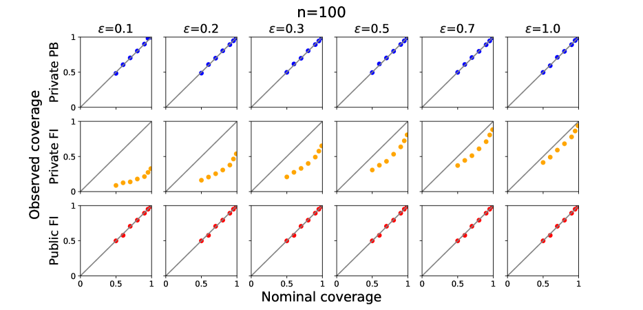
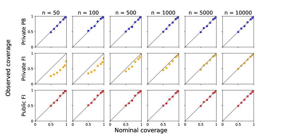
Figure 1: Observed vs nominal coverage of 95% CIs for different distributions for different n𝑛n.
Refer to caption
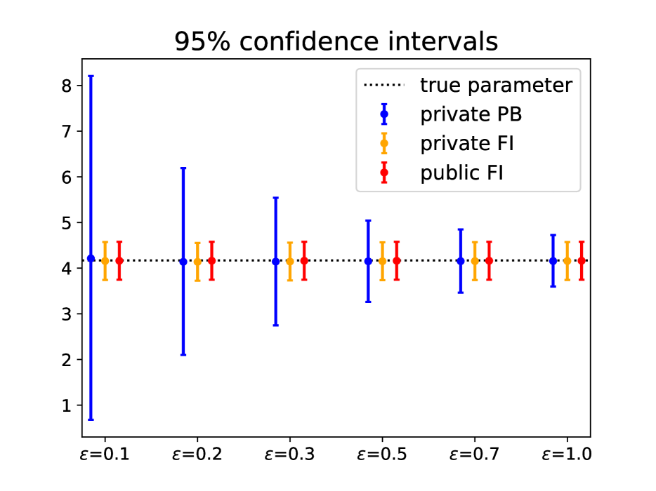
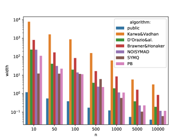
Figure 2: Left pair. (i) observed vs. nominal coverage for different coverage levels, for a Poisson, n=100, ϵ=0.5italic-ϵ0.5\epsilon=0.5. (ii) same plot, comparing the OPS method (Foulds et al., 2016) and the parametric bootstrap for Bernoulli estimation. Center pair: average CI widths for different n𝑛n for (i) Gamma and (ii) OLS (other distributions give qualitatively similar results). Width of the private bootstrap CIs approaches that of the public CIs as n𝑛n\rightarrow\infty. Right pair. (i) private and bias-corrected private estimates for a Poisson clamped at varying right-tail thresholds. (ii) same for a Gaussian clamped at 1010-10 on the left tail and at varying thresholds on the right tail.

We design synthetic experiments to demonstrate our proposed methods for differentially private confidence interval estimation.

First, we evaluate the performance of private parametric bootstrap CIs vs a baseline method (“Fisher CIs”) based on asymptotic normality of the private estimator and described in more detail below. Performance is measured by how well the coverage of the private CIs matches the nominal coverage. For all models, we also include Fisher CIs of non-private estimators for comparison.

Second, we demonstrate the bias-correction procedure in Sec. 3.1 in the case of Gaussian and Poisson distributions with data points clamped to different thresholds, which introduces estimation bias. These results show the effectiveness of the parametric bootstrap at approximating and mitigating the bias of differentially private estimates when sensitivity is bounded by forcing data to take values within given bounds.

Third, we compare parametric bootstrap CIs to another general purpose method to construct confidence intervals based on subsample & aggregate (Nissim et al., 2007; Smith, 2011; D’Orazio et al., 2015).

Finally, the appendix includes additional experiments exploring a broader range of settings and performance metrics. These include: multivariate distributions, the effect of varying ϵitalic-ϵ\epsilon, and measurements of the upper- and lower-tail CI failures. We aim for private CIs to be as tight as possible while providing the correct coverage: in the appendix, we also compare the width of our intervals with that of intervals from existing methods for the specific case of Gaussian mean estimation of known variance.

Baseline: “Fisher CIs”  As a byproduct of our consistency analysis we also derive asymptotic normal distributions of the private estimators for both exponential families (Theorem 2) and OLS (Theorem 3). In each case, we obtain a private, consistent estimate σ^j2subscriptsuperscript^𝜎2𝑗\hat{\sigma}^{2}_{j} of the j𝑗jth diagonal entry of the inverse Fisher information matrix of the private estimator θ^nsubscript^𝜃𝑛\hat{\theta}_{n}, and then construct the confidence interval for θjsubscript𝜃𝑗\theta_{j} as

Cn=[θ^n,jzα/2σ^j,θ^n,j+zα/2σ^j],subscript𝐶𝑛subscript^𝜃𝑛𝑗subscript𝑧𝛼2subscript^𝜎𝑗subscript^𝜃𝑛𝑗subscript𝑧𝛼2subscript^𝜎𝑗C_{n}=\big{[}\hat{\theta}_{n,j}-z_{\alpha/2}\hat{\sigma}_{j},\hat{\theta}_{n,j}+z_{\alpha/2}\hat{\sigma}_{j}\big{]}, (7)

where zγsubscript𝑧𝛾z_{\gamma} is the 1γ1𝛾1-\gamma-quantile of the standard normal distribution. For exponential families, the Fisher information is estimated via plug-in estimation with the private estimator θ^nsubscript^𝜃𝑛\hat{\theta}_{n}. For OLS, it is estimated via plugging in private estimates Q^n=1nXTX+1nVsubscript^𝑄𝑛1𝑛superscript𝑋𝑇𝑋1𝑛𝑉\hat{Q}_{n}=\frac{1}{n}X^{T}X+\frac{1}{n}V and σ^n2subscriptsuperscript^𝜎2𝑛\hat{\sigma}^{2}_{n}, which are both released by the SSP mechanism. For non-private Fisher CIs, we follow similar (and very standard) procedures with non-private estimators.

Exponential families  We use synthetic data sets drawn from different exponential family distributions. Given a family, true parameter θ𝜃\theta, and data size n𝑛n, a data set is drawn from Pθsubscript𝑃𝜃P_{\theta}. We release private statistics via SSP with the Laplace mechanism. To simulate the modeler’s domain knowledge about the data bounds, we draw a separate surrogate data set of size 1000 drawn from the same distribution, compute the data range and use it to bound the width of each released statistic. For private estimation, sampled data is clamped to this range. Private θ^^𝜃\hat{\theta} is computed from the privately released statistics using SSP-MLE. For the parametric bootstrap CIs, we implement Algorithm 1 and compute Efron’s percentile intervals (see Table 1). The output coverage is computed over T=1000𝑇1000T=1000 trials.

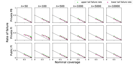
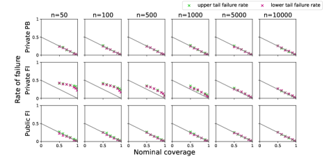
Results are shown in Figures 1 and 2. For the parametric bootstrap, actual coverage closely matches the nominal coverage, even for very small n𝑛n. Coverage of private Fisher CIs is too low until n𝑛n becomes large, due to the fact that it ignores privacy noise. The bootstrap procedure correctly accounts for the increased uncertainty due to the privacy by enlarging the CIs. The width of the bootstrap intervals approaches the width of the baseline Fisher intervals as n𝑛n\rightarrow\infty. In the appendix, we show that the coverage failures are balanced between left and right tails and examine the effect of increasing ϵitalic-ϵ\epsilon (which reduces privacy noise and has the same qualitative effect as increasing n𝑛n).

Linear regression  We follow a very similar procedure for OLS. Data is generated with xjUnif([5,5])similar-tosubscript𝑥𝑗Unif55x_{j}\sim\text{Unif}([-5,5]) for all j𝑗j and errors are uiUnif[10,10]similar-tosubscript𝑢𝑖Unif1010u_{i}\sim\text{Unif}[-10,10]; bounds on y𝑦y are passed as inputs ([150,150]150150[-150,150]) and assumed known. Observed values of y𝑦y exceeding the given bounds are dropped. These bounds are also used to compute widths for the sensitivity. Private coefficients are estimated with SSP-OLS and bootstrap CIs are constructed via Efron’s percentile method. The results are shown in Fig. 1.

Bias correction  In the case of distributions with infinite support, one option to bound the sensitivity is to clamp or truncate the data to given bounds. These procedures may induce estimation bias. As discussed in Sec 3.1, the parametric bootstrap can be used to approximate this bias and mitigate it. We demonstrate bias correction on the private estimates and CIs of a Poisson and Gaussian distribution where data is clamped on the right tail at different thresholds (Fig. 2).

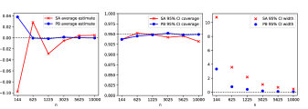
Comparison with subsample & aggregate  We compare the parametric bootstrap CIs with the intervals obtained via a subsample & aggregate (S&A) algorithm. We adapted the S&A procedure of D’Orazio et al. (2015) for privately estimating standard errors to compute confidence intervals; see Algorithm 2 in the appendix. We compare the accuracy of point estimates and 95% CIs for the mean of a Gaussian of known variance. We found that the parametric bootstrap provides more accurate point estimates and better calibrated, tighter CIs than S&A (Figure 3).
Refer to caption
Figure 3: Point estimates (left), 95% CI coverage (center) and average CI width (right) of the S&A method (see Algorithm 2 in appendix) vs parametric bootstrap for the mean of a Gaussian of known variance. Settings: ϵ=0.5italic-ϵ0.5\epsilon=0.5, θ=0𝜃0\theta=0, σ=1,(xmin,xmax)=(20,+20),(Lmin,Lmax)=(10,+10),varmax=50formulae-sequence𝜎1formulae-sequencesubscript𝑥𝑚𝑖𝑛subscript𝑥𝑚𝑎𝑥2020formulae-sequencesubscript𝐿𝑚𝑖𝑛subscript𝐿𝑚𝑎𝑥1010𝑣𝑎subscript𝑟𝑚𝑎𝑥50\sigma=1,(x_{min},x_{max})=(-20,+20),(L_{min},L_{max})=(-10,+10),var_{max}=50.

8 Conclusion

The parametric bootstrap is useful and effective to construct consistent differentially private confidence intervals for broad classes of private estimators, including private linear regression, for which we present a novel adaptation to avoid accessing the covariate data many times. The parametric bootstrap yields confidence intervals with good coverage even at modest sample sizes, and tighter than the ones based on subsample & aggregate or other general methods. It can be used with any privacy mechanism, and can help mitigate differentially private estimation bias.

References

  • Efron (1979) Bradley Efron. Bootstrap methods: Another look at the jackknife. Annals of Statistics, 7(1):1–26, 01 1979.
  • Brawner and Honaker (2018) Thomas Brawner and James Honaker. Bootstrap inference and differential privacy: Standard errors for free. Unpublished Manuscript, 2018.
  • Wang et al. (2015) Yu-Xiang Wang, Stephen Fienberg, and Alex Smola. Privacy for free: Posterior sampling and stochastic gradient monte carlo. In Proceedings of the 32nd International Conference on Machine Learning (ICML-15), pages 2493–2502, 2015.
  • Foulds et al. (2016) James Foulds, Joseph Geumlek, Max Welling, and Kamalika Chaudhuri. On the theory and practice of privacy-preserving bayesian data analysis. In Proceedings of the Thirty-Second Conference on Uncertainty in Artificial Intelligence, UAI’16, page 192–201, 2016.
  • Zhang et al. (2016) Zuhe Zhang, Benjamin I.P. Rubinstein, and Christos Dimitrakakis. On the differential privacy of bayesian inference. In Thirtieth AAAI Conference on Artificial Intelligence, 2016.
  • Dwork et al. (2006) Cynthia Dwork, Frank McSherry, Kobbi Nissim, and Adam Smith. Calibrating noise to sensitivity in private data analysis. In Theory of cryptography conference, pages 265–284. Springer, 2006.
  • Efron (1981a) Bradley Efron. Nonparametric standard errors and confidence intervals. Canadian Journal of Statistics, 9(2):139–158, 1981a.
  • Efron (1981b) Bradley Efron. Nonparametric estimates of standard error: the jackknife, the bootstrap and other methods. Biometrika, 68(3):589–599, 1981b.
  • Efron and Tibshirani (1986) Bradley Efron and Robert Tibshirani. Bootstrap methods for standard errors, confidence intervals, and other measures of statistical accuracy. Statistical science, pages 54–75, 1986.
  • Du et al. (2020) Wenxin Du, Canyon Foot, Monica Moniot, Andrew Bray, and Adam Groce. Differentially private confidence intervals. arXiv preprint arXiv:2001.02285, 2020. URL https://arxiv.org/abs/2001.02285.
  • Van der Vaart (2000) Aad W. Van der Vaart. Asymptotic statistics, volume 3. Cambridge university press, 2000.
  • Wasserman (2006) Larry Wasserman. All of nonparametric statistics. Springer Science & Business Media, 2006.
  • Efron and Hastie (2016) Bradley Efron and Trevor Hastie. Computer age statistical inference, volume 5. Cambridge University Press, 2016.
  • Gaboardi et al. (2016) Marco Gaboardi, Hyun Lim, Ryan Rogers, and Salil Vadhan. Differentially private chi-squared hypothesis testing: Goodness of fit and independence testing. In Proceedings of the 33rd International Conference on Machine Learning, volume 48, pages 2111–2120, 2016.
  • D’Orazio et al. (2015) Vito D’Orazio, James Honaker, and Gary King. Differential privacy for social science inference. Sloan Foundation Economics Research Paper, (2676160), 2015.
  • Wang et al. (2019) Yue Wang, Daniel Kifer, and Jaewoo Lee. Differentially private confidence intervals for empirical risk minimization. Journal of Privacy and Confidentiality, 9(1), 2019.
  • Evans et al. (2019) Georgina Evans, Gary King, Margaret Schwenzfeier, and Abhradeep Thakurta. Statistically valid inferences from privacy protected data. Working paper, 2019. URL https://gking.harvard.edu/files/gking/files/udpd.pdf.
  • Beran (1997) Rudolf Beran. Diagnosing bootstrap success. Annals of the Institute of Statistical Mathematics, 49(1):1–24, 1997.
  • Bernstein and Sheldon (2018) Garrett Bernstein and Daniel R. Sheldon. Differentially private bayesian inference for exponential families. In Advances in Neural Information Processing Systems, pages 2919–2929, 2018.
  • Davison (2003) Anthony C. Davison. Statistical models, volume 11. Cambridge University Press, 2003.
  • Wang (2018) Yu-Xiang Wang. Revisiting differentially private linear regression: optimal and adaptive prediction & estimation in unbounded domain, 2018.
  • Fox (2002) John Fox. An R and S-Plus companion to applied regression. Sage, 2002.
  • Dimitrakakis et al. (2014) Christos Dimitrakakis, Blaine Nelson, Aikaterini Mitrokotsa, and Benjamin I.P. Rubinstein. Robust and private bayesian inference. In International Conference on Algorithmic Learning Theory, pages 291–305. Springer, 2014.
  • Karwa and Vadhan (2018) Vishesh Karwa and Salil Vadhan. Finite sample differentially private confidence intervals. 9th Innovations in Theoretical Computer Science Conference, 2018.
  • Sheffet (2017) Or Sheffet. Differentially private ordinary least squares. In Proceedings of the 34th International Conference on Machine Learning, 2017.
  • Barrientos et al. (2018) Andrés F. Barrientos, Jerome P. Reiter, Ashwin Machanavajjhalab, and Yan Chen. Differentially private significance tests for regression coefficients. Journal of Computational and Graphical Statistics, 2018.
  • Gaboardi et al. (2019) Marco Gaboardi, Ryan Rogers, and Or Sheffet. Locally private mean estimation: z𝑧z-test and tight confidence intervals. In Kamalika Chaudhuri and Masashi Sugiyama, editors, Proceedings of Machine Learning Research, volume 89, pages 2545–2554, 2019.
  • Smith (2011) Adam Smith. Privacy-preserving statistical estimation with optimal convergence rates. In Proceedings of the forty-third annual ACM symposium on Theory of computing, pages 813–822, 2011.
  • Nissim et al. (2007) Kobbi Nissim, Sofya Raskhodnikova, and Adam Smith. Smooth sensitivity and sampling in private data analysis. In Proceedings of the thirty-ninth annual ACM symposium on Theory of computing, pages 75–84, 2007.
  • Vu and Slavkovic (2009) Duy Vu and Aleksandra Slavkovic. Differential privacy for clinical trial data: Preliminary evaluations. In 2009 IEEE International Conference on Data Mining Workshops, pages 138–143. IEEE, 2009.
  • Solea (2014) Eftychia Solea. Differentially private hypothesis testing for normal random variables. Master’s thesis, The Pennsylvania State University. 2014.
  • Couch et al. (2019) Simon Couch, Zeki Kazan, Kaiyan Shi, Andrew Bray, and Adam Groce. Differentially private nonparametric hypothesis testing. In Proceedings of the 2019 ACM SIGSAC Conference on Computer and Communications Security, pages 737–751, 2019.
  • Williams and McSherry (2010) Oliver Williams and Frank McSherry. Probabilistic inference and differential privacy. In Advances in Neural Information Processing Systems, pages 2451–2459, 2010.
  • Heikkilä et al. (2017) Mikko Heikkilä, Eemil Lagerspetz, Samuel Kaski, Kana Shimizu, Sasu Tarkoma, and Antti Honkela. Differentially private bayesian learning on distributed data. In Advances in neural information processing systems, pages 3226–3235, 2017.
  • Bernstein and Sheldon (2019) Garrett Bernstein and Daniel R. Sheldon. Differentially private bayesian linear regression. In Advances in Neural Information Processing Systems, pages 523–533, 2019.
  • King et al. (2020) Gary King et al. The OpenDP White Paper. Technical report, 2020.
  • Wang et al. (2018) Yue Wang, Daniel Kifer, Jaewoo Lee, and Vishesh Karwa. Statistical approximating distributions under differential privacy. Journal of Privacy and Confidentiality, 8(1), 2018.

Appendix A Proof of Claim 1

See 1

Proof.

Since X𝑋X and Xsuperscript𝑋X^{\prime} differ in exactly one element and f𝑓f is additive, f(X)f(X)=g(x)g(x)𝑓𝑋𝑓superscript𝑋𝑔𝑥𝑔superscript𝑥f(X)-f(X^{\prime})=g(x)-g(x^{\prime}) for some elements x,x𝑥superscript𝑥x,x^{\prime} in the data domain. The absolute value of the j𝑗jth output gj(x)gj(x)subscript𝑔𝑗𝑥subscript𝑔𝑗superscript𝑥g_{j}(x)-g_{j}(x^{\prime}) is bounded by width(gj)=maxxgj(x)minxgj(x)widthsubscript𝑔𝑗subscriptsuperscript𝑥subscript𝑔𝑗superscript𝑥subscriptsuperscript𝑥subscript𝑔𝑗superscript𝑥\operatorname{width}(g_{j})=\max_{x^{*}}g_{j}(x^{*})-\min_{x^{*}}g_{j}(x^{*}). The L1subscript𝐿1L_{1} sensitivity f(X)f(X)1=g(x)g(x)1subscriptnorm𝑓𝑋𝑓superscript𝑋1subscriptnorm𝑔𝑥𝑔superscript𝑥1\|f(X)-f(X^{\prime})\|_{1}=\|g(x)-g(x)^{\prime}\|_{1} is therefore at most the sum of the widths. ∎

Appendix B Proofs for Bootstrap Theory

See 1

This theorem is a simplified version of the result of Beran (1997). We give a self-contained proof. See also (Van der Vaart, 2000, Problem 23.5).

Proof.

The distribution of n(τ^nτ)𝑛subscript^𝜏𝑛𝜏\sqrt{n}(\hat{\tau}_{n}-\tau) under θsubscript𝜃\mathbb{P}_{\theta} is Hn(θ)subscript𝐻𝑛𝜃H_{n}(\theta), which, by asymptotic equivariance, converges to H(θ)𝐻𝜃H(\theta). In the parametric bootstrap, the distribution of n(τ^nτ^n)𝑛subscriptsuperscript^𝜏𝑛subscript^𝜏𝑛\sqrt{n}(\hat{\tau}^{*}_{n}-\hat{\tau}_{n}) conditional on θ^n=θ+hn/nsubscript^𝜃𝑛𝜃subscript𝑛𝑛\hat{\theta}_{n}=\theta+h_{n}/\sqrt{n} is Hn(θ+hn/n))H_{n}(\theta+h_{n}/\sqrt{n})), and, by asymptotic equivariance, Hn(θ+hn/n))H(θ)H_{n}(\theta+h_{n}/\sqrt{n}))\rightsquigarrow H(\theta) if hnsubscript𝑛h_{n} is convergent. Since H(θ)𝐻𝜃H(\theta) is continuous this is equivalent to saying that, for all convergent sequences hnsubscript𝑛h_{n} and all t𝑡t

n(n(τ^nτ^n)tθ^n=θ+hn/n)Fθ(t).subscriptsuperscript𝑛𝑛subscriptsuperscript^𝜏𝑛subscript^𝜏𝑛conditional𝑡subscript^𝜃𝑛𝜃subscript𝑛𝑛subscript𝐹𝜃𝑡\mathbb{P}^{*}_{n}\left(\sqrt{n}(\hat{\tau}^{*}_{n}-\hat{\tau}_{n})\leq t\mid\hat{\theta}_{n}=\theta+h_{n}/\sqrt{n}\right)\rightarrow F_{\theta}(t). (8)

where Fθsubscript𝐹𝜃F_{\theta} is the CDF of H(θ)𝐻𝜃H(\theta). Now, let h^n=n(θ^nθ)subscript^𝑛𝑛subscript^𝜃𝑛𝜃\hat{h}_{n}=\sqrt{n}(\hat{\theta}_{n}-\theta) so that θ^n=θ+h^n/nsubscript^𝜃𝑛𝜃subscript^𝑛𝑛\hat{\theta}_{n}=\theta+\hat{h}_{n}/\sqrt{n}. By assumption, h^nJ(θ)subscript^𝑛𝐽𝜃\hat{h}_{n}\rightsquigarrow J(\theta) and is therefore OP(1)subscript𝑂𝑃1O_{P}(1). Therefore, by Lemma 3, Eq. (8) implies

n(n(τ^nτ^n)tθ^n)Fθ(t) in θ-probabilitysuperscriptsubscript𝑛𝑛subscriptsuperscript^𝜏𝑛subscript^𝜏𝑛conditional𝑡subscript^𝜃𝑛subscript𝐹𝜃𝑡 in θ-probability\mathbb{P}_{n}^{*}\left(\sqrt{n}(\hat{\tau}^{*}_{n}-\hat{\tau}_{n})\leq t\mid\hat{\theta}_{n}\right)\rightarrow F_{\theta}(t)\text{ in $\mathbb{P}_{\theta}$-probability}

and the result is proved. ∎

Lemma 3.

Suppose gnsubscript𝑔𝑛g_{n} is a sequence of functions such that gn(hn)0subscript𝑔𝑛subscript𝑛0g_{n}(h_{n})\to 0 for any fixed sequence hn=O(1)subscript𝑛𝑂1h_{n}=O(1). Then gn(h^n)P0superscript𝑃subscript𝑔𝑛subscript^𝑛0g_{n}(\hat{h}_{n})\stackrel{{\scriptstyle P}}{{\to}}0 for every random sequence h^n=OP(1)subscript^𝑛subscript𝑂𝑃1\hat{h}_{n}=O_{P}(1).

Proof.

Fix ϵ,δ>0italic-ϵ𝛿0\epsilon,\delta>0. We wish to show, for large enough n𝑛n, that

Pr[|gn(h^n)|>ϵ]<δ.Prsubscript𝑔𝑛subscript^𝑛italic-ϵ𝛿\Pr\big{[}|g_{n}(\hat{h}_{n})|>\epsilon\big{]}<\delta.

Since h^nsubscript^𝑛\hat{h}_{n} is OP(1)subscript𝑂𝑃1O_{P}(1), there is some M𝑀M such that, for all n𝑛n,

Pr[hn>M]<δ.Prnormsubscript𝑛𝑀𝛿\Pr\big{[}\|h_{n}\|>M\big{]}<\delta.

By our assumption on gnsubscript𝑔𝑛g_{n}, there is some N𝑁N such that |gn(h)|<ϵsubscript𝑔𝑛italic-ϵ|g_{n}(h)|<\epsilon for all hM,n>Nformulae-sequencenorm𝑀𝑛𝑁\|h\|\leq M,n>N (take the sequence hnhsubscript𝑛h_{n}\equiv h for each such hh). Then, for n>N𝑛𝑁n>N,

Pr[|gn(h^n)|>ϵ]Pr[hn>M]<δ.Prsubscript𝑔𝑛subscript^𝑛italic-ϵPrnormsubscript𝑛𝑀𝛿\Pr\big{[}|g_{n}(\hat{h}_{n})|>\epsilon\big{]}\leq\Pr\big{[}\|h_{n}\|>M\big{]}<\delta.

Appendix C Proofs for Exponential Families

Lemma 4.

Let w𝑤w be any random variable with mean zero and finite variance. For any r>0𝑟0r>0, 1NrwP0superscript𝑃1superscript𝑁𝑟𝑤0\frac{1}{N^{r}}w\stackrel{{\scriptstyle P}}{{\to}}0.

Proof.

The variance of Nrwsuperscript𝑁𝑟𝑤N^{-r}w is equal to N2rVar(w)superscript𝑁2𝑟Var𝑤N^{-2r}\operatorname*{Var}(w), which goes to zero as N𝑁N\to\infty. By Chebyshev’s inequality, this implies that Nrw𝑃0superscript𝑁𝑟𝑤𝑃0N^{-r}w\overset{P}{\to}0. ∎

See 2

Following standard practice, we will prove this for the case when θ𝜃\theta is scalar; the generalization to vector θ𝜃\theta is straightforward but cumbersome. We first state the required (standard) regularity conditions. Let

n(θ)=i=1n(θ;xi)=i=1n(logp(xi;θ)logh(x))=θi=1nT(xi)nA(θ)subscript𝑛𝜃superscriptsubscript𝑖1𝑛𝜃subscript𝑥𝑖superscriptsubscript𝑖1𝑛𝑝subscript𝑥𝑖𝜃𝑥𝜃superscriptsubscript𝑖1𝑛𝑇subscript𝑥𝑖𝑛𝐴𝜃\begin{split}\ell_{n}(\theta)&=\sum_{i=1}^{n}\ell(\theta;x_{i})=\sum_{i=1}^{n}\big{(}\log p(x_{i};\theta)-\log h(x)\big{)}\\ &=\theta\sum_{i=1}^{n}T(x_{i})-nA(\theta)\end{split}

be the log-likelihood of a sample x1:nsubscript𝑥:1𝑛x_{1\mathrel{\mathop{\mathchar 58\relax}}n} from the exponential family model using the definition of log-likelihood from Sec. 1. Let (θ)=1(θ)𝜃subscript1𝜃\ell(\theta)=\ell_{1}(\theta) be the log-likelihood of a single xp(x;θ)similar-to𝑥𝑝𝑥𝜃x\sim p(x;\theta).

We assume the log-likelihood satisfies the conditions given in the book of Davison (2003, Section 4.4.2). If it does, then we have the following

  1. (F1)

    𝔼θ[(θ)]=0subscript𝔼𝜃superscript𝜃0\operatorname*{\mathbb{E}}_{\theta}[\ell^{\prime}(\theta)]=0.

  2. (F2)

    Varθ[(θ)]=𝔼θ[′′(θ)]=I(θ)subscriptVar𝜃superscript𝜃subscript𝔼𝜃superscript′′𝜃𝐼𝜃\operatorname*{Var}_{\theta}[\ell^{\prime}(\theta)]=-\operatorname*{\mathbb{E}}_{\theta}[\ell^{\prime\prime}(\theta)]=I(\theta).

  3. (F3)

    Given a sequence of estimators θ^nPθsuperscript𝑃subscript^𝜃𝑛𝜃\hat{\theta}_{n}\stackrel{{\scriptstyle P}}{{\to}}\theta, for all θ~n[θ,θ^n]subscript~𝜃𝑛𝜃subscript^𝜃𝑛\tilde{\theta}_{n}\in[\theta,\hat{\theta}_{n}], 12nn′′′(θ~n)(θ^nθ)2P0superscript𝑃12𝑛subscriptsuperscript′′′𝑛subscript~𝜃𝑛superscriptsubscript^𝜃𝑛𝜃20\;\frac{1}{2\sqrt{n}}\ell^{\prime\prime\prime}_{n}(\tilde{\theta}_{n})(\hat{\theta}_{n}-\theta)^{2}\stackrel{{\scriptstyle P}}{{\to}}0

Facts (F1) and (F2) are well known exponential family properties. Also recall that, for an exponential family,

  1. (F4)

    I(θ)=A′′(θ)𝐼𝜃superscript𝐴′′𝜃I(\theta)=A^{\prime\prime}(\theta).

  2. (F5)

    ′′(θ)superscript′′𝜃-\ell^{\prime\prime}(\theta) is deterministic and equal to I(θ)𝐼𝜃I(\theta).

Proof.

Let λn(θ)=f(θ,w+i=1nT(xi))subscript𝜆𝑛𝜃𝑓𝜃𝑤superscriptsubscript𝑖1𝑛𝑇subscript𝑥𝑖\lambda_{n}(\theta)=f\big{(}\theta,w+\sum_{i=1}^{n}T(x_{i})\big{)} be the objective of the SSP-MLE optimization problem. We have

λn(θ)subscript𝜆𝑛𝜃\displaystyle\lambda_{n}(\theta) =θ(w+i=1nT(xi))nA(θ)absent𝜃𝑤superscriptsubscript𝑖1𝑛𝑇subscript𝑥𝑖𝑛𝐴𝜃\displaystyle=\theta\Big{(}w+\sum_{i=1}^{n}T(x_{i})\Big{)}-nA(\theta)
=θw+θi=1nT(xi)nA(θ)absent𝜃𝑤𝜃superscriptsubscript𝑖1𝑛𝑇subscript𝑥𝑖𝑛𝐴𝜃\displaystyle=\theta w+\theta\sum_{i=1}^{n}T(x_{i})-nA(\theta)
=θw+n(θ)absent𝜃𝑤subscript𝑛𝜃\displaystyle=\theta w+\ell_{n}(\theta)

where n(θ)subscript𝑛𝜃\ell_{n}(\theta) is the log-likelihood of the true sample. That is, the original objective n(θ)subscript𝑛𝜃\ell_{n}(\theta) is perturbed by the linear function θw𝜃𝑤\theta w to obtain λn(θ)subscript𝜆𝑛𝜃\lambda_{n}(\theta). The derivatives are therefore related as:

λn(θ)superscriptsubscript𝜆𝑛𝜃\displaystyle\lambda_{n}^{\prime}(\theta) =w+n(θ),absent𝑤subscriptsuperscript𝑛𝜃\displaystyle=w+\ell^{\prime}_{n}(\theta), (9)
λn(k)(θ)superscriptsubscript𝜆𝑛𝑘𝜃\displaystyle\lambda_{n}^{(k)}(\theta) =(k)(θ),k>1.formulae-sequenceabsentsuperscript𝑘𝜃𝑘1\displaystyle=\ell^{(k)}(\theta),\quad k>1. (10)

At the optimum θ^nsubscript^𝜃𝑛\hat{\theta}_{n}, the first derivative of λnsubscript𝜆𝑛\lambda_{n} is equal to zero. (θ)superscript𝜃\ell^{\prime}(\theta) is a sum of i.i.d. terms with mean 00 and variance I(θ)𝐼𝜃I(\theta), more specifically:

(θ)=i=1n(T(xi)A(θ))superscript𝜃superscriptsubscript𝑖1𝑛𝑇subscript𝑥𝑖superscript𝐴𝜃\ell^{\prime}(\theta)=\sum_{i=1}^{n}\left(T(x_{i})-A^{\prime}(\theta)\right)

For asymptotic equivariance, we are interested in the sequence of estimators θ^nsubscript^𝜃𝑛\hat{\theta}_{n} when the “true parameter” follows the sequence θ+hn/n𝜃subscript𝑛𝑛\theta+h_{n}/\sqrt{n}. We follow the standard approach of writing the Taylor expansion of the first derivative about the true parameter θ+hn/n𝜃subscript𝑛𝑛\theta+h_{n}/\sqrt{n}:

0=w+n(θ+hn/n)+n′′(θ+hn/n)(θ^nθhn/n)+Zn0𝑤subscriptsuperscript𝑛𝜃subscript𝑛𝑛subscriptsuperscript′′𝑛𝜃subscript𝑛𝑛subscript^𝜃𝑛𝜃subscript𝑛𝑛subscript𝑍𝑛0=w+\ell^{\prime}_{n}(\theta+h_{n}/\sqrt{n})+\ell^{\prime\prime}_{n}(\theta+h_{n}/\sqrt{n})(\hat{\theta}_{n}-\theta-h_{n}/\sqrt{n})+Z_{n} (11)

where we have used Eqs. (9) and (10) to replace the derivatives of λ𝜆\lambda on the right-hand side, and Zn=12n′′′(θ~n)(θ^nθhn/n)2subscript𝑍𝑛12subscriptsuperscript′′′𝑛subscript~𝜃𝑛superscriptsubscript^𝜃𝑛𝜃subscript𝑛𝑛2Z_{n}=\tfrac{1}{2}\ell^{\prime\prime\prime}_{n}(\tilde{\theta}_{n})(\hat{\theta}_{n}-\theta-h_{n}/\sqrt{n})^{2} is the second-order Taylor term, with θ~nsubscript~𝜃𝑛\tilde{\theta}_{n} some point in the interval [θ+hn/n,θ^n]𝜃subscript𝑛𝑛subscript^𝜃𝑛[\theta+h_{n}/\sqrt{n},\hat{\theta}_{n}].

Multiply both sides of the equation by 1n1𝑛\frac{1}{\sqrt{n}} and rearrange to get

n(θ^nθhn/n)=1nw+1nn(θ+hn/n)+1nZn1nn′′(θ+hn/n)=1nw+1nn(θ+hn/n)+1nZnI(θ+hn/n)𝑛subscript^𝜃𝑛𝜃subscript𝑛𝑛1𝑛𝑤1𝑛subscriptsuperscript𝑛𝜃subscript𝑛𝑛1𝑛subscript𝑍𝑛1𝑛subscriptsuperscript′′𝑛𝜃subscript𝑛𝑛1𝑛𝑤1𝑛subscriptsuperscript𝑛𝜃subscript𝑛𝑛1𝑛subscript𝑍𝑛𝐼𝜃subscript𝑛𝑛\begin{split}\sqrt{n}(\hat{\theta}_{n}-\theta-h_{n}/\sqrt{n})&=\frac{\frac{1}{\sqrt{n}}w+\frac{1}{\sqrt{n}}\ell^{\prime}_{n}(\theta+h_{n}/\sqrt{n})+\frac{1}{\sqrt{n}}Z_{n}}{-\frac{1}{n}\ell^{\prime\prime}_{n}(\theta+h_{n}/\sqrt{n})}\\ &=\frac{\frac{1}{\sqrt{n}}w+\frac{1}{\sqrt{n}}\ell^{\prime}_{n}(\theta+h_{n}/\sqrt{n})+\frac{1}{\sqrt{n}}Z_{n}}{I(\theta+h_{n}/\sqrt{n})}\end{split}

where in the second equality we used (F5). By Lemma 4, 1nwP0superscript𝑃1𝑛𝑤0\frac{1}{\sqrt{n}}w\stackrel{{\scriptstyle P}}{{\to}}0 and by (F3) 1nZnP0superscript𝑃1𝑛subscript𝑍𝑛0\frac{1}{\sqrt{n}}Z_{n}\stackrel{{\scriptstyle P}}{{\to}}0, so, by Slutsky,

n(θ^nθhn/n)P1n(θ+hnn)I(θ+hnn)=(θ+hnn)nI(θ+hnn)(B)1I(θ+hnn)superscript𝑃𝑛subscript^𝜃𝑛𝜃subscript𝑛𝑛1𝑛superscript𝜃subscript𝑛𝑛𝐼𝜃subscript𝑛𝑛subscriptsuperscript𝜃subscript𝑛𝑛𝑛𝐼𝜃subscript𝑛𝑛𝐵1𝐼𝜃subscript𝑛𝑛\sqrt{n}(\hat{\theta}_{n}-\theta-h_{n}/\sqrt{n})\stackrel{{\scriptstyle P}}{{\to}}\frac{\frac{1}{\sqrt{n}}\ell^{\prime}(\theta+\frac{h_{n}}{\sqrt{n}})}{I(\theta+\frac{h_{n}}{\sqrt{n}})}=\underbrace{\frac{\ell^{\prime}(\theta+\frac{h_{n}}{\sqrt{n}})}{\sqrt{nI(\theta+\frac{h_{n}}{\sqrt{n}})}}}_{(B)}\frac{1}{\sqrt{I(\theta+\frac{h_{n}}{\sqrt{n}})}} (12)

We know that under the regularity assumptions the Fisher information I()𝐼I(\cdot) is a continuous function and so, since θ+hnnθ𝜃subscript𝑛𝑛𝜃\theta+\frac{h_{n}}{\sqrt{n}}\to\theta, then by continuity (I()𝐼I(\cdot) is deterministic):

(I(θ+hnn))1/2(I(θ))1/2superscript𝐼𝜃subscript𝑛𝑛12superscript𝐼𝜃12\displaystyle\left(I\left(\theta+\frac{h_{n}}{\sqrt{n}}\right)\right)^{-1/2}\to\left(I(\theta)\right)^{-1/2}

We now focus on the asymptotic behavior of (B)𝐵(B). We will use the fact that in exponential families, 𝔼θT(x)=A(θ)subscript𝔼𝜃𝑇𝑥superscript𝐴𝜃\operatorname*{\mathbb{E}}_{\theta}T(x)=A^{\prime}(\theta) and VarθT(x)=A′′(θ)=I(θ)subscriptVar𝜃𝑇𝑥superscript𝐴′′𝜃𝐼𝜃\operatorname*{Var}_{\theta}T(x)=A^{\prime\prime}(\theta)=I(\theta). For simplicity of notation, define:

μn=A(θ+hnn).subscript𝜇𝑛superscript𝐴𝜃subscript𝑛𝑛\mu_{n}=A^{\prime}\left(\theta+\frac{h_{n}}{\sqrt{n}}\right).

Define now the triangular array written in the following notation:

T(x1)μ1x1θ+h11similar-to𝑇subscript𝑥1subscript𝜇1subscript𝑥1subscript𝜃subscript11\displaystyle T(x_{1})-\mu_{1}\hskip 142.26378ptx_{1}\sim\mathbb{P}_{\theta+\frac{h_{1}}{1}}
T(x1)μ2,T(x2)μ2x1:2i.i.d.θ+h22\displaystyle T(x_{1})-\mu_{2},T(x_{2})-\mu_{2}\hskip 85.35826ptx_{1\mathrel{\mathop{\mathchar 58\relax}}2}\overset{i.i.d.}{\sim}\mathbb{P}_{\theta+\frac{h_{2}}{\sqrt{2}}}
T(x1)μ3,T(x2)μ3,T(x3)μ3x1:3i.i.d.θ+h33\displaystyle T(x_{1})-\mu_{3},T(x_{2})-\mu_{3},T(x_{3})-\mu_{3}\hskip 34.14322ptx_{1\mathrel{\mathop{\mathchar 58\relax}}3}\overset{i.i.d.}{\sim}\mathbb{P}_{\theta+\frac{h_{3}}{\sqrt{3}}}
\displaystyle...\hskip 199.16928pt...
T(x1)μn,T(x2)μn,,T(xn)μnx1:ni.i.d.θ+hnn\displaystyle T(x_{1})-\mu_{n},T(x_{2})-\mu_{n},...,T(x_{n})-\mu_{n}\hskip 17.07182ptx_{1\mathrel{\mathop{\mathchar 58\relax}}n}\overset{i.i.d.}{\sim}\mathbb{P}_{\theta+\frac{h_{n}}{\sqrt{n}}}

Let’s focus on the n𝑛n-th row. By construction the sum over the n𝑛n-th row is Sn=i=1n(T(xi)μn)=(θ+hnn)subscript𝑆𝑛superscriptsubscript𝑖1𝑛𝑇subscript𝑥𝑖subscript𝜇𝑛superscript𝜃subscript𝑛𝑛S_{n}=\sum_{i=1}^{n}(T(x_{i})-\mu_{n})=\ell^{\prime}(\theta+\frac{h_{n}}{\sqrt{n}}), so the numerator of (A)𝐴(A). Each term in the n𝑛n-th row has mean zero and:

σn2=i=1nVar[T(xi)μn]=nI(θ+hnn).subscriptsuperscript𝜎2𝑛superscriptsubscript𝑖1𝑛Var𝑇subscript𝑥𝑖subscript𝜇𝑛𝑛𝐼𝜃subscript𝑛𝑛\sigma^{2}_{n}=\sum_{i=1}^{n}\operatorname*{Var}[T(x_{i})-\mu_{n}]=nI\left(\theta+\frac{h_{n}}{\sqrt{n}}\right).

If for every ϵ>0italic-ϵ0\epsilon>0 the following condition holds:

limn1σn2i=1n𝔼[(T(xi)μn)2𝟏(|T(xi)μn|ϵσn)]=0,subscript𝑛1subscriptsuperscript𝜎2𝑛superscriptsubscript𝑖1𝑛𝔼delimited-[]superscript𝑇subscript𝑥𝑖subscript𝜇𝑛21𝑇subscript𝑥𝑖subscript𝜇𝑛italic-ϵsubscript𝜎𝑛0\lim_{n\to\infty}\frac{1}{\sigma^{2}_{n}}\sum_{i=1}^{n}\mathbb{E}\left[(T(x_{i})-\mu_{n})^{2}\mathbf{1}\left(\mathinner{\!\left\lvert T(x_{i})-\mu_{n}\right\rvert}\geq\epsilon\sigma_{n}\right)\right]=0,

then Sn/σn𝒩(0,1)subscript𝑆𝑛subscript𝜎𝑛𝒩01S_{n}/\sigma_{n}\to\mathcal{N}(0,1) by the Lindeberg-Feller Central Limit Theorem. By plugging in the terms in the condition above we have that:

limnsubscript𝑛\displaystyle\lim_{n\to\infty} 1nI(θ+hnn)i=1n𝔼[(T(xi)μn)2𝟏(|T(xi)μn|ϵnI(θ+hnn))]1𝑛𝐼𝜃subscript𝑛𝑛superscriptsubscript𝑖1𝑛𝔼delimited-[]superscript𝑇subscript𝑥𝑖subscript𝜇𝑛21𝑇subscript𝑥𝑖subscript𝜇𝑛italic-ϵ𝑛𝐼𝜃subscript𝑛𝑛\displaystyle\frac{1}{nI\left(\theta+\frac{h_{n}}{\sqrt{n}}\right)}\sum_{i=1}^{n}\mathbb{E}\left[(T(x_{i})-\mu_{n})^{2}\mathbf{1}\left(\mathinner{\!\left\lvert T(x_{i})-\mu_{n}\right\rvert}\geq\epsilon\sqrt{n}\sqrt{I\left(\theta+\frac{h_{n}}{\sqrt{n}}\right)}\right)\right]
=limnI(θ+hnn)1𝔼[(T(x1)μn)2𝟏(|T(x1)μn|ϵnI(θ+hnn))]absentsubscript𝑛𝐼superscript𝜃subscript𝑛𝑛1𝔼delimited-[]superscript𝑇subscript𝑥1subscript𝜇𝑛21𝑇subscript𝑥1subscript𝜇𝑛italic-ϵ𝑛𝐼𝜃subscript𝑛𝑛\displaystyle=\lim_{n\to\infty}I\left(\theta+\frac{h_{n}}{\sqrt{n}}\right)^{-1}\mathbb{E}\left[(T(x_{1})-\mu_{n})^{2}\mathbf{1}\left(\mathinner{\!\left\lvert T(x_{1})-\mu_{n}\right\rvert}\geq\epsilon\sqrt{n}\sqrt{I\left(\theta+\frac{h_{n}}{\sqrt{n}}\right)}\right)\right]

with the equality due to i.i.d. sampling within the row of the triangular array. Note that for any x1subscript𝑥1x_{1},

limn(T(x1)μn)2𝟏(|T(x1)μn|ϵnI(θ+hnn))=0,subscript𝑛superscript𝑇subscript𝑥1subscript𝜇𝑛21𝑇subscript𝑥1subscript𝜇𝑛italic-ϵ𝑛𝐼𝜃subscript𝑛𝑛0\lim_{n\to\infty}(T(x_{1})-\mu_{n})^{2}\mathbf{1}\left(\mathinner{\!\left\lvert T(x_{1})-\mu_{n}\right\rvert}\geq\epsilon\sqrt{n}\sqrt{I\left(\theta+\frac{h_{n}}{\sqrt{n}}\right)}\right)=0,

and that the integrand above is dominated by (T(x1)μn)2superscript𝑇subscript𝑥1subscript𝜇𝑛2(T(x_{1})-\mu_{n})^{2}, which is integrable and finite, since 𝔼[(T(x1)μn)2]𝔼delimited-[]superscript𝑇subscript𝑥1subscript𝜇𝑛2\mathbb{E}[(T(x_{1})-\mu_{n})^{2}] is finite. Hence by the dominated convergence theorem, the limit is zero and the condition is satisfied.

Going back to equation (12), we then have that

1n(θ+hnn)I(θ+hnn)𝒩(0,1)(I(θ))1/2=𝒩(0,I(θ)1),1𝑛superscript𝜃subscript𝑛𝑛𝐼𝜃subscript𝑛𝑛𝒩01superscript𝐼𝜃12𝒩0𝐼superscript𝜃1\frac{\frac{1}{\sqrt{n}}\ell^{\prime}(\theta+\frac{h_{n}}{\sqrt{n}})}{I(\theta+\frac{h_{n}}{\sqrt{n}})}\rightsquigarrow\mathcal{N}(0,1)\cdot\left(I(\theta)\right)^{-1/2}=\mathcal{N}(0,I(\theta)^{-1}),

which proves that n(θ^nθhn/n)𝒩(0,I(θ)1)𝑛subscript^𝜃𝑛𝜃subscript𝑛𝑛𝒩0𝐼superscript𝜃1\sqrt{n}(\hat{\theta}_{n}-\theta-h_{n}/\sqrt{n})\rightsquigarrow\mathcal{N}(0,I(\theta)^{-1}). Setting hn=0subscript𝑛0h_{n}=0, it is straightforward to find that n(θ^nθ)𝒩(0,I(θ)1)𝑛subscript^𝜃𝑛𝜃𝒩0𝐼superscript𝜃1\sqrt{n}(\hat{\theta}_{n}-\theta)\rightsquigarrow\mathcal{N}(0,I(\theta)^{-1}). This proves that SSP-MLE is asymptotically equivariant. ∎

Appendix D Proofs for OLS

See 3

Before proving the theorem, we give two lemmas. The first is standard and describes the asymptotics of the dominant term.

Lemma 5.

Under the assumptions of the OLS model in Section 5, 1nXT𝐮𝒩(0,σ2Q)1𝑛superscript𝑋𝑇𝐮𝒩0superscript𝜎2𝑄\frac{1}{\sqrt{n}}X^{T}\mathbf{u}\rightsquigarrow\mathcal{N}(0,\sigma^{2}Q).

Proof.

Observe that XT𝐮=i=1n𝐱iuisuperscript𝑋𝑇𝐮superscriptsubscript𝑖1𝑛subscript𝐱𝑖subscript𝑢𝑖X^{T}\mathbf{u}=\sum_{i=1}^{n}\mathbf{x}_{i}u_{i} is a sum of iid terms, and, using the assumptions of the model in Section 1, the mean and variance of the terms are 𝔼[𝐱iui]=𝔼[𝐱i]𝔼[ui]=0𝔼subscript𝐱𝑖subscript𝑢𝑖𝔼subscript𝐱𝑖𝔼subscript𝑢𝑖0\operatorname*{\mathbb{E}}[\mathbf{x}_{i}u_{i}]=\operatorname*{\mathbb{E}}[\mathbf{x}_{i}]\operatorname*{\mathbb{E}}[u_{i}]=0 and Var(𝐱iui)=Var(𝐱u)=𝔼[𝐱uu𝐱T]=𝔼[u2𝐱𝐱T]=𝔼[u2]𝔼[𝐱𝐱T]=σ2QVarsubscript𝐱𝑖subscript𝑢𝑖Var𝐱𝑢𝔼𝐱𝑢𝑢superscript𝐱𝑇𝔼superscript𝑢2superscript𝐱𝐱𝑇𝔼superscript𝑢2𝔼superscript𝐱𝐱𝑇superscript𝜎2𝑄\operatorname*{Var}(\mathbf{x}_{i}u_{i})=\operatorname*{Var}(\mathbf{x}u)=\operatorname*{\mathbb{E}}[\mathbf{x}uu\mathbf{x}^{T}]=\operatorname*{\mathbb{E}}[u^{2}\mathbf{x}\mathbf{x}^{T}]=\operatorname*{\mathbb{E}}[u^{2}]\operatorname*{\mathbb{E}}[\mathbf{x}\mathbf{x}^{T}]=\sigma^{2}Q. The result follows from the central limit theorem. ∎

The theorem involves asymptotic statements about β^nsubscript^𝛽𝑛\hat{\beta}_{n} and β^nsubscriptsuperscript^𝛽𝑛\hat{\beta}^{*}_{n}. The following lemma is a general asymptotic result that will apply to both estimators using Eqs. (6) and (5).

Lemma 6.

Define the function

n{Qˇ,βˇ,Zˇ,Vˇ,wˇ}=(Qˇ+1nVˇ)1Qˇβˇ+(Qˇ+1nVˇ)1(1nZˇ+1nwˇ)subscript𝑛ˇ𝑄ˇ𝛽ˇ𝑍ˇ𝑉ˇ𝑤superscriptˇ𝑄1𝑛ˇ𝑉1ˇ𝑄ˇ𝛽superscriptˇ𝑄1𝑛ˇ𝑉11𝑛ˇ𝑍1𝑛ˇ𝑤\mathcal{B}_{n}\{\check{Q},\check{\beta},\check{Z},\check{V},\check{w}\}=\left(\check{Q}+\frac{1}{n}\check{V}\right)^{-1}\check{Q}\check{\beta}+\left(\check{Q}+\frac{1}{n}\check{V}\right)^{-1}\left(\frac{1}{\sqrt{n}}\check{Z}+\frac{1}{n}\check{w}\right)

and suppose the sequences Qn,βn,Zn,Vn,wnsubscript𝑄𝑛subscript𝛽𝑛subscript𝑍𝑛subscript𝑉𝑛subscript𝑤𝑛Q_{n},\beta_{n},Z_{n},V_{n},w_{n} are defined on a common probability space and satisfy

  1. (i)

    Zn𝒩(0,σ2Q)subscript𝑍𝑛𝒩0superscript𝜎2𝑄Z_{n}\rightsquigarrow\mathcal{N}(0,\sigma^{2}Q),

  2. (ii)

    QnPQsuperscript𝑃subscript𝑄𝑛𝑄Q_{n}\stackrel{{\scriptstyle P}}{{\to}}Q,

  3. (iii)

    βn,Vn,wnsubscript𝛽𝑛subscript𝑉𝑛subscript𝑤𝑛\beta_{n},V_{n},w_{n} are all OP(1)subscript𝑂𝑃1O_{P}(1).

Then

n(n{Qn,βn,Zn,Vn,wn}βn)𝒩(0,σ2Q1).𝑛subscript𝑛subscript𝑄𝑛subscript𝛽𝑛subscript𝑍𝑛subscript𝑉𝑛subscript𝑤𝑛subscript𝛽𝑛𝒩0superscript𝜎2superscript𝑄1\sqrt{n}\Big{(}\mathcal{B}_{n}\{Q_{n},\beta_{n},Z_{n},V_{n},w_{n}\}-\beta_{n}\Big{)}\rightsquigarrow\mathcal{N}(0,\sigma^{2}Q^{-1}).
Proof.

Substitute the sequences into nsubscript𝑛\mathcal{B}_{n} and rearrange to get

n(nβn)=n((Qn+1nVn)1QnI)βn+n(Qn+1nVn)1(1nZn+1nwn)𝑛subscript𝑛subscript𝛽𝑛𝑛superscriptsubscript𝑄𝑛1𝑛subscript𝑉𝑛1subscript𝑄𝑛𝐼subscript𝛽𝑛𝑛superscriptsubscript𝑄𝑛1𝑛subscript𝑉𝑛11𝑛subscript𝑍𝑛1𝑛subscript𝑤𝑛\displaystyle\sqrt{n}\left(\mathcal{B}_{n}-\beta_{n}\right)=\sqrt{n}\left(\left(Q_{n}+\frac{1}{n}V_{n}\right)^{-1}Q_{n}-I\right)\beta_{n}+\sqrt{n}\left(Q_{n}+\frac{1}{n}V_{n}\right)^{-1}\left(\frac{1}{\sqrt{n}}Z_{n}+\frac{1}{n}w_{n}\right) (13)

First, note that the sequences 1nVn1𝑛subscript𝑉𝑛\frac{1}{n}V_{n}, 1nVn1𝑛subscript𝑉𝑛\frac{1}{\sqrt{n}}V_{n} and 1nwn1𝑛subscript𝑤𝑛\frac{1}{\sqrt{n}}w_{n}, which will appear below, are all oP(1)subscript𝑜𝑃1o_{P}(1), since Vnsubscript𝑉𝑛V_{n} and wnsubscript𝑤𝑛w_{n} are OP(1)subscript𝑂𝑃1O_{P}(1).

The first term in Eq. (13) converges to zero in probability. Specifically, a manipulation shows:

n((Qn+1nVn)1QnI)βn𝑛superscriptsubscript𝑄𝑛1𝑛subscript𝑉𝑛1subscript𝑄𝑛𝐼subscript𝛽𝑛\displaystyle\sqrt{n}\left(\left(Q_{n}+\frac{1}{n}V_{n}\right)^{-1}Q_{n}-I\right)\beta_{n} =(Qn+1nVn)1(1nVn)βnabsentsuperscriptsubscript𝑄𝑛1𝑛subscript𝑉𝑛11𝑛subscript𝑉𝑛subscript𝛽𝑛\displaystyle=\left(Q_{n}+\frac{1}{n}V_{n}\right)^{-1}\left(-\frac{1}{\sqrt{n}}V_{n}\right)\beta_{n}
=OP(1)oP(1)OP(1)absentsubscript𝑂𝑃1subscript𝑜𝑃1subscript𝑂𝑃1\displaystyle=O_{P}(1)o_{P}(1)O_{P}(1)
=oP(1)absentsubscript𝑜𝑃1\displaystyle=o_{P}(1)

For the first factor on the right side, (Qn+1nVn)1PQ1superscript𝑃superscriptsubscript𝑄𝑛1𝑛subscript𝑉𝑛1superscript𝑄1(Q_{n}+\frac{1}{n}V_{n})^{-1}\stackrel{{\scriptstyle P}}{{\to}}Q^{-1} (by Slutsky’s theorem, since QnPQsuperscript𝑃subscript𝑄𝑛𝑄Q_{n}\stackrel{{\scriptstyle P}}{{\to}}Q and 1nVnP0superscript𝑃1𝑛subscript𝑉𝑛0\frac{1}{n}V_{n}\stackrel{{\scriptstyle P}}{{\to}}0), and is therefore OP(1)subscript𝑂𝑃1O_{P}(1). For the second factor, we argued 1nVn=oP(1)1𝑛subscript𝑉𝑛subscript𝑜𝑃1-\frac{1}{\sqrt{n}}V_{n}=o_{P}(1). For the third factor, βn=OP(1)subscript𝛽𝑛subscript𝑂𝑃1\beta_{n}=O_{P}(1) by assumption.

The second term in Eq. (13) converges in distribution to 𝒩(0,σ2Q)𝒩0superscript𝜎2𝑄\mathcal{N}(0,\sigma^{2}Q). Rewrite it as

(Qn+1nVn)1(Zn+1nwn).superscriptsubscript𝑄𝑛1𝑛subscript𝑉𝑛1subscript𝑍𝑛1𝑛subscript𝑤𝑛\left(Q_{n}+\frac{1}{n}V_{n}\right)^{-1}\left(Z_{n}+\frac{1}{\sqrt{n}}w_{n}\right).

We already argued that (Qn+1nVn)1PQ1superscript𝑃superscriptsubscript𝑄𝑛1𝑛subscript𝑉𝑛1superscript𝑄1(Q_{n}+\frac{1}{n}V_{n})^{-1}\stackrel{{\scriptstyle P}}{{\to}}Q^{-1} and 1nwnP0superscript𝑃1𝑛subscript𝑤𝑛0\frac{1}{\sqrt{n}}w_{n}\stackrel{{\scriptstyle P}}{{\to}}0. By assumption, Zn𝒩(0,σ2Q)subscript𝑍𝑛𝒩0superscript𝜎2𝑄Z_{n}\rightsquigarrow\mathcal{N}(0,\sigma^{2}Q). Therefore, by Slutsky’s theorem, the entire term converges in distribution to Q1𝒩(0,σ2Q)=𝒩(0,σ2Q1)superscript𝑄1𝒩0superscript𝜎2𝑄𝒩0superscript𝜎2superscript𝑄1Q^{-1}\mathcal{N}(0,\sigma^{2}Q)=\mathcal{N}(0,\sigma^{2}Q^{-1}). ∎

We are ready to prove the Theorem 3.

Proof of Theorem 3.

We first wish to show that n(β^nβ)𝒩(0,σ2Q1)𝑛subscript^𝛽𝑛𝛽𝒩0superscript𝜎2superscript𝑄1\sqrt{n}\left(\hat{\beta}_{n}-\beta\right)\rightsquigarrow\mathcal{N}(0,\sigma^{2}Q^{-1}). To see this, write β^n=n{1nXTX,β,1nXT𝐮,V,w}subscript^𝛽𝑛subscript𝑛1𝑛superscript𝑋𝑇𝑋𝛽1𝑛superscript𝑋𝑇𝐮𝑉𝑤\hat{\beta}_{n}=\mathcal{B}_{n}\left\{\frac{1}{n}X^{T}X,\beta,\frac{1}{\sqrt{n}}X^{T}\mathbf{u},V,w\right\} and apply Lemma 6. It is easy to verify that the sequences satisfy the conditions of the lemma.

Next, we wish to show that the bootstrap estimator is consistent. By Lemma 1, it is enough to show that n(β^nβ^n)𝒩(0,σ2Q1)𝑛subscriptsuperscript^𝛽𝑛subscript^𝛽𝑛𝒩0superscript𝜎2superscript𝑄1\sqrt{n}(\hat{\beta}^{*}_{n}-\hat{\beta}_{n})\rightsquigarrow\mathcal{N}(0,\sigma^{2}Q^{-1}) conditional on ω𝜔\omega in θsubscript𝜃\mathbb{P}_{\theta}-probability, where θ=(β,σ2,Q)𝜃𝛽superscript𝜎2𝑄\theta=(\beta,\sigma^{2},Q) and θsubscript𝜃\mathbb{P}_{\theta} is the common probability space of the data and privacy random variables, represented by ω𝜔\omega. The bootstrap variables Zn,V,wsubscriptsuperscript𝑍𝑛superscript𝑉superscript𝑤Z^{*}_{n},V^{*},w^{*} correspond to the inner measure nsubscriptsuperscript𝑛\mathbb{P}^{*}_{n}. Define Q^n=1nXTX+1nVsubscript^𝑄𝑛1𝑛superscript𝑋𝑇𝑋1𝑛𝑉\hat{Q}_{n}=\frac{1}{n}X^{T}X+\frac{1}{n}V. Observe that Eq. (5) is equivalent to

β^n=n{Q^n,β^n,Zn,V,w}under Zn𝒩(0,σ^n2Q^n),VFV,wFw,formulae-sequencesubscriptsuperscript^𝛽𝑛subscript𝑛subscript^𝑄𝑛subscript^𝛽𝑛subscriptsuperscript𝑍𝑛superscript𝑉superscript𝑤formulae-sequencesimilar-tounder subscriptsuperscript𝑍𝑛𝒩0subscriptsuperscript^𝜎2𝑛subscript^𝑄𝑛formulae-sequencesimilar-tosuperscript𝑉subscript𝐹𝑉similar-tosuperscript𝑤subscript𝐹𝑤\hat{\beta}^{*}_{n}=\mathcal{B}_{n}\{\hat{Q}_{n},\hat{\beta}_{n},Z^{*}_{n},V^{*},w^{*}\}\ \ \text{under }Z^{*}_{n}\sim\mathcal{N}(0,\hat{\sigma}^{2}_{n}\hat{Q}_{n}),V^{*}\sim F_{V},w^{*}\sim F_{w}, (14)

and (Q^n,β^n,σ^2)subscript^𝑄𝑛subscript^𝛽𝑛superscript^𝜎2(\hat{Q}_{n},\hat{\beta}_{n},\hat{\sigma}^{2}) are consistent estimators and hence converge in θsubscript𝜃\mathbb{P}_{\theta}-probability to (Q,β,σ2)𝑄𝛽superscript𝜎2(Q,\beta,\sigma^{2}).

We can’t apply Lemma 6 directly to Eq.(14) because this expression mixes random variables from the outer space (Q^n,β^n,σ^n2subscript^𝑄𝑛subscript^𝛽𝑛subscriptsuperscript^𝜎2𝑛\hat{Q}_{n},\hat{\beta}_{n},\hat{\sigma}^{2}_{n}) and inner space (Zn,V,w)subscriptsuperscript𝑍𝑛superscript𝑉superscript𝑤(Z^{*}_{n},V^{*},w^{*}). Instead, we temporarily reason about a deterministic sequence (Qn,βn,σn2)(Q,β,σ2)subscript𝑄𝑛subscript𝛽𝑛subscriptsuperscript𝜎2𝑛𝑄𝛽superscript𝜎2(Q_{n},\beta_{n},\sigma^{2}_{n})\to(Q,\beta,\sigma^{2}). Then, by Lemma 6 applied to the inner probability space,

n(n{Qn,βn,Zn,V,w}βn)𝒩(0,σ2Q1)under Zn𝒩(0,σn2Qn),VPV,wPwformulae-sequence𝑛subscript𝑛subscript𝑄𝑛subscript𝛽𝑛subscriptsuperscript𝑍𝑛superscript𝑉superscript𝑤subscript𝛽𝑛𝒩0superscript𝜎2superscript𝑄1under subscriptsuperscript𝑍𝑛similar-to𝒩0subscriptsuperscript𝜎2𝑛subscript𝑄𝑛formulae-sequencesimilar-tosuperscript𝑉subscript𝑃𝑉similar-tosuperscript𝑤subscript𝑃𝑤\begin{split}\sqrt{n}\Big{(}\mathcal{B}_{n}\{Q_{n},\beta_{n},Z^{*}_{n},V^{*},w^{*}\}-\beta_{n}\Big{)}\rightsquigarrow\mathcal{N}(0,\sigma^{2}Q^{-1})\\ \text{under }Z^{*}_{n}\sim\mathcal{N}(0,\sigma^{2}_{n}Q_{n}),V^{*}\sim P_{V},w^{*}\sim P_{w}\end{split} (15)

The conditions of Lemma 6 can easily be checked. In particular, we have Zn𝒩(0,σ2Q)subscriptsuperscript𝑍𝑛𝒩0superscript𝜎2𝑄Z^{*}_{n}\rightsquigarrow\mathcal{N}(0,\sigma^{2}Q).

We can restate the result Eq. (15) as follows: for any fixed sequence (Qn,βn,σn2)(Q,β,σ2)subscript𝑄𝑛subscript𝛽𝑛subscriptsuperscript𝜎2𝑛𝑄𝛽superscript𝜎2(Q_{n},\beta_{n},\sigma^{2}_{n})\to(Q,\beta,\sigma^{2}) and all t𝑡t,

n(n(β^nβ^n)tQ^n=Qn,β^n=βn,σ^n2=σn)F(t)\mathbb{P}^{*}_{n}\left(\sqrt{n}(\hat{\beta}^{*}_{n}-\hat{\beta}_{n})\leq t\mid\hat{Q}_{n}=Q_{n},\hat{\beta}_{n}=\beta_{n},\hat{\sigma}^{2}_{n}=\sigma_{n}\right)\to F(t)

where F𝐹F is the CDF of 𝒩(0,σ2Q1)𝒩0superscript𝜎2superscript𝑄1\mathcal{N}(0,\sigma^{2}Q^{-1}). Lemma 7 below now implies that

n(n(β^nβ^n)tQ^n,β^n,σ^n2)F(t) in θ-probability,subscriptsuperscript𝑛𝑛subscriptsuperscript^𝛽𝑛subscript^𝛽𝑛conditional𝑡subscript^𝑄𝑛subscript^𝛽𝑛subscriptsuperscript^𝜎2𝑛𝐹𝑡 in θ-probability\mathbb{P}^{*}_{n}\left(\sqrt{n}(\hat{\beta}^{*}_{n}-\hat{\beta}_{n})\leq t\mid\hat{Q}_{n},\hat{\beta}_{n},\hat{\sigma}^{2}_{n}\right)\to F(t)\text{ in $\mathbb{P}_{\theta}$-probability},

and the theorem is proved. ∎

Lemma 7.

Let gn:k:subscript𝑔𝑛superscript𝑘superscriptg_{n}\mathrel{\mathop{\mathchar 58\relax}}\mathbb{R}^{k}\to\mathbb{R}^{\ell} be a sequence of functions such that gn(hn)csubscript𝑔𝑛subscript𝑛𝑐g_{n}(h_{n})\to c for any deterministic sequence hnhsubscript𝑛h_{n}\to h. Then gn(h^n)Pcsuperscript𝑃subscript𝑔𝑛subscript^𝑛𝑐g_{n}(\hat{h}_{n})\stackrel{{\scriptstyle P}}{{\to}}c for any random sequence h^nPhsuperscript𝑃subscript^𝑛\hat{h}_{n}\stackrel{{\scriptstyle P}}{{\to}}h.

Proof.

Take c=0𝑐0c=0 without loss of generality, let \|\cdot\| be any norm and d(x,y)=xy𝑑𝑥𝑦norm𝑥𝑦d(x,y)=\|x-y\|. Fix ϵ>0italic-ϵ0\epsilon>0. It must be the case that

δ>0,n0 such that: d(h,h)<δgn(h)<ϵ,nn0.formulae-sequenceformulae-sequence𝛿0formulae-sequencesubscript𝑛0 such that: 𝑑superscript𝛿normsubscript𝑔𝑛superscriptitalic-ϵfor-all𝑛subscript𝑛0\exists\,\delta>0,n_{0}\in\mathbb{N}\text{ such that: }\quad d(h^{\prime},h)<\delta\implies\|g_{n}(h^{\prime})\|<\epsilon,\forall n\geq n_{0}. (16)

Otherwise, we can construct a convergent sequence hnhsubscript𝑛h_{n}\to h with lim supngn(hn)ϵsubscriptlimit-supremum𝑛normsubscript𝑔𝑛subscript𝑛italic-ϵ\limsup_{n\to\infty}\|g_{n}(h_{n})\|\geq\epsilon, which violates the conditions of the Lemma.666If Eq. (16) is not true, then for all δ>0𝛿0\delta>0 and n0subscript𝑛0n_{0}\in\mathbb{N}, there exists hsuperscripth^{\prime} such that d(h,h)<δ𝑑superscript𝛿d(h^{\prime},h)<\delta and gn(h)ϵnormsubscript𝑔𝑛superscriptitalic-ϵ\|g_{n}(h^{\prime})\|\geq\epsilon for some nn0𝑛subscript𝑛0n\geq n_{0}. Then we can construct a sequence hnhsubscript𝑛h_{n}\to h as follows. Let δksubscript𝛿𝑘\delta_{k} be any sequence such that δk0subscript𝛿𝑘0\delta_{k}\to 0. Set n0=0subscript𝑛00n_{0}=0, and, for k1𝑘1k\geq 1, select hsuperscripth^{\prime} such that d(h,h)<δk𝑑superscriptsubscript𝛿𝑘d(h^{\prime},h)<\delta_{k} and gn(h)ϵnormsubscript𝑔superscript𝑛superscriptitalic-ϵ\|g_{n^{\prime}}(h^{\prime})\|\geq\epsilon for some nnk1+1superscript𝑛subscript𝑛𝑘11n^{\prime}\geq n_{k-1}+1. Set hn=hsubscript𝑛superscripth_{n}=h^{\prime} for all n{nk1+1,,n}𝑛subscript𝑛𝑘11superscript𝑛n\in\{n_{k-1}+1,\ldots,n^{\prime}\} and let nk=nsubscript𝑛𝑘superscript𝑛n_{k}=n^{\prime}. This sequence satisfies hnhsubscript𝑛h_{n}\to h but gnk(hnk)ϵsubscript𝑔subscript𝑛𝑘subscriptsubscript𝑛𝑘italic-ϵg_{n_{k}}(h_{n_{k}})\geq\epsilon for all k𝑘k, so it is not true that gn(hn)0subscript𝑔𝑛subscript𝑛0g_{n}(h_{n})\to 0. This contradicts the assumptions of the lemma, so Eq. (16) must be true.

Now, suppose h^nPhsuperscript𝑃subscript^𝑛\hat{h}_{n}\stackrel{{\scriptstyle P}}{{\to}}h. Then, for nn0𝑛subscript𝑛0n\geq n_{0}, by Eq. (16),

Pr[gn(h^n)>ϵ]Pr[d(h^n,h)>δ].Prnormsubscript𝑔𝑛subscript^𝑛italic-ϵPr𝑑subscript^𝑛𝛿\Pr\left[\|g_{n}(\hat{h}_{n})\|>\epsilon\right]\leq\Pr\left[d(\hat{h}_{n},h)>\delta\right].

Therefore

limnPr[gn(h^n)>ϵ]limnPr[d(h^n,h)>δ]=0,subscript𝑛Prnormsubscript𝑔𝑛subscript^𝑛italic-ϵsubscript𝑛Pr𝑑subscript^𝑛𝛿0\lim_{n\to\infty}\Pr\left[\|g_{n}(\hat{h}_{n})\|>\epsilon\right]\leq\lim_{n\to\infty}\Pr\left[d(\hat{h}_{n},h)>\delta\right]=0,

which proves the result. ∎

Appendix E Subsample & Aggregate

Algorithm 2 Subsample&Aggregate

Input X,M,xmin,xmax,Lmin,Lmax,varmax,ϵ,α𝑋𝑀subscript𝑥𝑚𝑖𝑛subscript𝑥𝑚𝑎𝑥subscript𝐿𝑚𝑖𝑛subscript𝐿𝑚𝑎𝑥𝑣𝑎subscript𝑟𝑚𝑎𝑥italic-ϵ𝛼X,M,x_{min},x_{max},L_{min},L_{max},var_{max},\epsilon,\alpha

1:procedure SubsampleAndAggregate
2:     X1,,XMsubsample(X,M)subscript𝑋1subscript𝑋𝑀subsample𝑋𝑀X_{1},...,X_{M}\leftarrow\textbf{subsample}(X,M)
3:     Lmin,LmaxLminN/M,LmaxN/Mformulae-sequencesubscriptsuperscript𝐿𝑚𝑖𝑛subscriptsuperscript𝐿𝑚𝑎𝑥subscript𝐿𝑚𝑖𝑛𝑁𝑀subscript𝐿𝑚𝑎𝑥𝑁𝑀L^{*}_{min},L^{*}_{max}\leftarrow\frac{L_{min}}{\sqrt{N/M}},\frac{L_{max}}{\sqrt{N/M}}
4:     varmaxvarmaxN/M𝑣𝑎subscriptsuperscript𝑟𝑚𝑎𝑥𝑣𝑎subscript𝑟𝑚𝑎𝑥𝑁𝑀var^{*}_{max}\leftarrow\frac{var_{max}}{N/M}
5:     for i=1,,M𝑖1𝑀i=1,...,M do
6:         c^iclamp(𝒜(Xi),Lmin,Lmax)subscript^𝑐𝑖clamp𝒜subscript𝑋𝑖subscriptsuperscript𝐿𝑚𝑖𝑛subscriptsuperscript𝐿𝑚𝑎𝑥\hat{c}_{i}\leftarrow\textbf{clamp}(\mathcal{A}(X_{i}),L^{*}_{min},L^{*}_{max})      
7:     Δ1|LmaxLmin|MsubscriptΔ1subscriptsuperscript𝐿𝑚𝑎𝑥subscriptsuperscript𝐿𝑚𝑖𝑛𝑀\Delta_{1}\leftarrow\frac{|L^{*}_{max}-L^{*}_{min}|}{M}
8:     θ^DP1Mi=1Mc^i+Lap(0,Δ1ϵ/2)subscript^𝜃𝐷𝑃1𝑀superscriptsubscript𝑖1𝑀subscript^𝑐𝑖Lap0subscriptΔ1italic-ϵ2\hat{\theta}_{DP}\leftarrow\frac{1}{M}\sum_{i=1}^{M}\hat{c}_{i}+\text{Lap}(0,\frac{\Delta_{1}}{\epsilon/2})
9:     for i=1,,M𝑖1𝑀i=1,...,M do
10:         for b=1,,B𝑏1𝐵b=1,...,B do
11:              Xi,bresample(Xi,NM,replace=True)subscript𝑋𝑖𝑏resamplesubscript𝑋𝑖𝑁𝑀replace=TrueX_{i,b}\leftarrow\textbf{resample}(X_{i},\lfloor\frac{N}{M}\rfloor,\text{replace=True})
12:              c^i,bclamp(𝒜(Xi,b),Lmin,Lmax)subscript^𝑐𝑖𝑏clamp𝒜subscript𝑋𝑖𝑏subscriptsuperscript𝐿𝑚𝑖𝑛subscriptsuperscript𝐿𝑚𝑎𝑥\hat{c}_{i,b}\leftarrow\textbf{clamp}(\mathcal{A}(X_{i,b}),L^{*}_{min},L^{*}_{max})          
13:         var^c^iclamp(Var(c^i,1:B),106,varmax)subscript^𝑣𝑎𝑟subscript^𝑐𝑖clampVarsubscript^𝑐:𝑖1𝐵superscript106𝑣𝑎subscriptsuperscript𝑟𝑚𝑎𝑥\hat{var}_{\hat{c}_{i}}\leftarrow\textbf{clamp}(\operatorname*{Var}(\hat{c}_{i,1\mathrel{\mathop{\mathchar 58\relax}}B}),10^{-6},var^{*}_{max})      
14:     Δ2varmax/MsubscriptΔ2𝑣𝑎subscriptsuperscript𝑟𝑚𝑎𝑥𝑀\Delta_{2}\leftarrow var^{*}_{max}/M
15:     var^c^1Mi=1Mvar^c^i+Lap(0,Δ2ϵ/2)subscript^𝑣𝑎𝑟^𝑐1𝑀superscriptsubscript𝑖1𝑀subscript^𝑣𝑎𝑟subscript^𝑐𝑖Lap0subscriptΔ2italic-ϵ2\hat{var}_{\hat{c}}\leftarrow\frac{1}{M}\sum_{i=1}^{M}\hat{var}_{\hat{c}_{i}}+\text{Lap}(0,\frac{\Delta_{2}}{\epsilon/2})
16:     var^DP1Mvar^c^+Var(Lap(0,Δ1ϵ/2))subscript^𝑣𝑎𝑟𝐷𝑃1𝑀subscript^𝑣𝑎𝑟^𝑐VarLap0subscriptΔ1italic-ϵ2\hat{var}_{DP}\leftarrow\frac{1}{M}\hat{var}_{\hat{c}}+\operatorname*{Var}(\text{Lap}(0,\frac{\Delta_{1}}{\epsilon/2}))
17:     CIDP[θ^DPzα2var^DP,θ^DP+zα2var^DP]subscriptCI𝐷𝑃subscript^𝜃𝐷𝑃subscript𝑧𝛼2subscript^𝑣𝑎𝑟𝐷𝑃subscript^𝜃𝐷𝑃subscript𝑧𝛼2subscript^𝑣𝑎𝑟𝐷𝑃\text{CI}_{DP}\leftarrow[\hat{\theta}_{DP}-z_{\frac{\alpha}{2}}\sqrt{\hat{var}_{DP}},\hat{\theta}_{DP}+z_{\frac{\alpha}{2}}\sqrt{\hat{var}_{DP}}] return θ^DP,CIDPsubscript^𝜃𝐷𝑃subscriptCI𝐷𝑃\hat{\theta}_{DP},\text{CI}_{DP}

Appendix F Additional Experiments
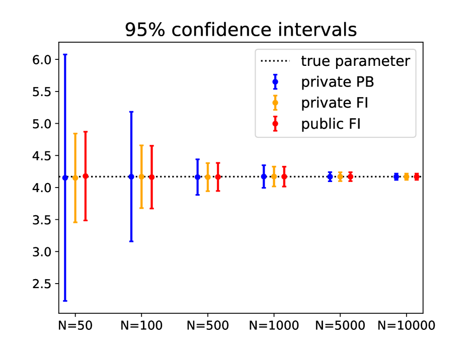
Refer to caption
(a)
Refer to caption
(b)
Figure 4: Effects of varying ϵitalic-ϵ\epsilon for a fixed n=100𝑛100n=100. We selected a Gamma with inference on the scale parameter. The results are qualitatively equivalent for other distributions. (a) Observed coverage vs. nominal coverage of CIs. Coverage levels: {0.5,0.6,0.7,0.8,0.9,0.95,0.99}0.50.60.70.80.90.950.99\{0.5,0.6,0.7,0.8,0.9,0.95,0.99\}. From top to bottom: (i) differentially private parametric bootstrap; (ii) differentially private Fisher intervals; (iii) non-private Fisher CIs. Private methods use SSP via Laplace mechanism with varying values of ϵitalic-ϵ\epsilon. Note that the effect of increasing ϵitalic-ϵ\epsilon with n𝑛n fixed is qualitatively similar to the effect of increasing n𝑛n holding ϵitalic-ϵ\epsilon fixed. (b) Average CIs for the scale parameter for different ϵitalic-ϵ\epsilon. The width of the private bootstrap CIs approaches that of the public CIs as ϵitalic-ϵ\epsilon increases.
Refer to caption
Refer to caption
Figure 5: In this Figure, we look at the rate of failure of the confidence intervals on the upper vs lower tail. For each of the two plots, the rows represent (i) differentially private parametric bootstrap; (ii) differentially private Fisher intervals; (iii) non-private Fisher intervals. Top: data range and sensitivity computed as described in Section 7. Clamping the data to a range can introduce a bias if the range is not conservative enough. The bias becomes noticeable for large n𝑛n, where the interval width is smaller. In our case, where the range is approximated from a data set of size 1000, a small bias becomes noticeable for n5000𝑛5000n\geq 5000, where upper-tail failures systematically outnumber lower-tail failures by a small margin. Bottom: same as top plot, with double the range. Increasing the range mitigates the bias.
Refer to caption
(a)
Refer to caption
(b)
Figure 6: Observed vs nominal coverage (left) and average CI width (right) for a multivariate Gaussian in 5 dimensions, with ϵ=0.5italic-ϵ0.5\epsilon=0.5. We compute CIs for each dimension separately and report results for the first dimension as an example.
Refer to caption
Figure 7: For different algorithms, average width (logscale) of differentially private confidence intervals for the mean of a standard normal, range [8,8]88[-8,8], ϵ=0.1italic-ϵ0.1\epsilon=0.1, for different n𝑛n levels. “public” is the confidence interval computed without differential privacy; “Karwa&Vadhan” refers to Karwa and Vadhan (2018); “D’Orazio&al.” refers to D’Orazio et al. (2015); “Brawner&Honaker” refers to Brawner and Honaker (2018); “NOISYMAD" and “SYMQ” are methods from Du et al. (2020), and in particular “NOISYMAD” is very similar to our parametric bootstrap method (“PB”). We used the publicly available implementation by Du et al. (2020) to reproduce their methods as well as the other prior methods.