Optimal Transport Kernels for Sequential and Parallel
Neural Architecture Search

Abstract

Neural architecture search (NAS) automates the design of deep neural networks. One of the main challenges in searching complex and non-continuous architectures is to compare the similarity of networks that the conventional Euclidean metric may fail to capture. Optimal transport (OT) is resilient to such complex structure by considering the minimal cost for transporting a network into another. However, the OT is generally not negative definite which may limit its ability to build the positive-definite kernels required in many kernel-dependent frameworks. Building upon tree-Wasserstein (TW), which is a negative definite variant of OT, we develop a novel discrepancy for neural architectures, and demonstrate it within a Gaussian process (GP) surrogate model for the sequential NAS settings. Furthermore, we derive a novel parallel NAS, using quality k-determinantal point process on the GP posterior, to select diverse and high-performing architectures from a discrete set of candidates. We empirically demonstrate that our TW-based approaches outperform other baselines in both sequential and parallel NAS.

1 Introduction

Neural architecture search (NAS) is the process of automating architecture engineering to find the best design of our neural network model. This output architecture will perform well for a given dataset. With the increasing interest in deep learning in recent years, NAS has attracted significant research attention (Dong & Yang, 2019; Elsken et al., 2019a; Liu et al., 2018, 2019; Luo et al., 2018; Real et al., 2019, 2017; Shah et al., 2018; Suganuma et al., 2017; Xie & Yuille, 2017; Yao et al., 2020). We refer the interested readers to the survey (Elsken et al., 2019b) for a detailed review of NAS and to the comprehensive list for all of the related papers in NAS.

Bayesian optimization (BO) utilizes a probabilistic model, particularly Gaussian process (GP) (Rasmussen, 2006), for determining future evaluations and its evaluation efficiency makes it well suited for the expensive evaluations of NAS. However, the conventional BO approaches (Shahriari et al., 2016; Snoek et al., 2012) are not suitable to capture the complex and non-continuous designs of neural architectures. Recent work (Kandasamy et al., 2018) has considered optimal transport (OT) for measuring neural architectures. This views two networks as logistical suppliers and receivers, then optimizes to find the minimal transportation cost as the distance, i.e., similar architectures will need less cost for transporting and vice versa. However, the existing OT distance for architectures, such as OTMANN (Kandasamy et al., 2018), do not easily lend themselves to the creation of the positive semi-definite (p.s.d.) kernel (covariance function) due to the indefinite property of OT (Peyré & Cuturi, 2019) (§8.3). It is critical as the GP is not a valid random process when the covariance function (kernel) is not p.s.d. (see Lem. 2.1). In addition, there is still an open research direction for parallel NAS where the goal is to select multiple high-performing and diverse candidates from a discrete set of candidates for parallel evaluations. This discrete property makes the parallel NAS interesting and different from the existing batch BO approaches (Desautels et al., 2014; González et al., 2016), which are typically designed to handle continuous observations.

We propose a negative definite tree-Wasserstein (TW) distance for neural network architectures based on a novel design which captures both global and local information via $n$-gram and indegree/outdegree representations for networks. In addition, we propose the k-determinantal point process (k-DPP) quality for selecting diverse and high-performing architectures from a discrete set. This discrete property of NAS makes k-DPP ideal in sampling the choices overcoming the greedy selection used in the existing batch Bayesian optimization (Desautels et al., 2014; González et al., 2016; Wang et al., 2018). At a high level, our contributions are three-fold as follows:

• A TW distance with a novel design for capturing both local and global information from architectures which results in a p.s.d. kernel while the existing OT distance does not.

• A demonstration of TW as the novel GP covariance function for sequential NAS.

• A parallel NAS approach using k-DPP for selecting diverse and high-quality architectures from a discrete set.

2 Tree-Wasserstein for Neural Network Architectures

We first argue that the covariance matrices associated with a kernel function of Gaussian process (GP) and k-DPP need to be positive semi-definite (p.s.d.) for a valid random process in Lemma 2.1. We then develop tree-Wasserstein (TW) (Do Ba et al., 2011; Le et al., 2019b), the negative definite variant of optimal transport (OT), for measuring the similarity of architectures. Consequently, we can build a p.s.d. kernel upon OT geometry for modeling with GPs and k-determinantal point processes (k-DPPs).

Lemma 2.1.

If a covariance function $k$ of a Gaussian process is not positive semi-definite, the resulting GP is not a valid random process.

Proof of Lemma 2.1 is placed in the Appendix §D.1.

2.1 Tree-Wasserstein

We give a brief review about OT, tree metric, tree-Wasserstein (TW) which are the main components for our NAS framework. We denote $[n]=\{1,2,\ldots,n\}$, $\forall n\in\mathbb{N}_{+}$. Let $(\Omega,d)$ be a measurable metric space. For any $x\in\Omega$, we use $\delta_{x}$ for the Dirac unit mass on $x$.

Optimal transport.

OT, a.k.a. Wasserstein, Monge-Kantorovich, or Earth Mover’s distance, is the flexible tool to compare probability measures (Peyré & Cuturi, 2019; Villani, 2003). Let $\omega$, $\nu$ be Borel probability distributions on $\Omega$ and $\mathcal{R}(\omega,\nu)$ be the set of probability distributions $\pi$ on $\Omega\times\Omega$ such that $\pi(B\times\Omega)=\omega(B)$ and $\pi(\Omega\times B^{\prime})=\nu(B^{\prime})$ for all Borel sets $B$, $B^{\prime}$. The 1-Wasserstein distance $W_{d}$ (Villani, 2003) (p.2) between $\omega$ and $\nu$ is defined as:

$$W_{d}(\omega,\nu)=\inf_{\pi\in\mathcal{R}(\omega,\nu)}\int_{\Omega\times\Omega}d(x,z)\pi(\textnormal{d}x,\textnormal{d}z),$$ (1)

where $d$ is a ground metric (i.e., cost metric) of OT.

Tree metrics and tree-Wasserstein.

A metric $d:\Omega\times\Omega\rightarrow\mathbb{R}_{+}$ is a tree metric if there exists a tree $\mathcal{T}$ with positive edge lengths such that $\forall x\in\Omega$, then $x$ is a node of $\mathcal{T}$; and $\forall x,z\in\Omega$, $d(x,z)$ is equal to the length of the (unique) path between $x$ and $z$ (Semple & Steel, 2003) (§7, p.145–182).

Let $d_{\mathcal{T}}$ be the tree metric on tree $\mathcal{T}$ rooted at $r$. For $x,z\in\mathcal{T}$, we denote $\mathcal{P}(x,z)$ as the (unique) path between $x$ and $z$. We write $\Gamma(x)$ for a set of nodes in the subtree of $\mathcal{T}$ rooted at $x$, defined as $\Gamma(x)=\bigl{\{}z\in\mathcal{T}\mid x\in\mathcal{P}(r,z)\bigr{\}}$. For edge $e$ in $\mathcal{T}$, let $v_{e}$ be the deeper level node of edge $e$ (the farther node to root $r$), and $w_{e}$ be the positive length of that edge.

Tree-Wasserstein (TW) is a special case of OT whose ground metric is a tree metric (Do Ba et al., 2011; Le et al., 2019b). Given two measures $\omega$, $\nu$ supported on tree $\mathcal{T}$, and setting the tree metric $d_{\mathcal{T}}$ as the ground metric, then the TW distance $W_{d_{\mathcal{T}}}$ between $\omega$ and $\nu$ admits a closed-form solution as follows:

$$W_{d_{\mathcal{T}}}(\omega,\nu)=\sum_{e\in\mathcal{T}}w_{e}\bigl{|}\omega\bigl{(}\Gamma(v_{e})\bigr{)}-\nu\bigl{(}\Gamma(v_{e})\bigr{)}\bigr{|},$$ (2)

where $\omega(\Gamma(v_{e}))$ is the total mass of the probability measure $\omega$ in the subtree $\Gamma(v_{e})$ rooted at $v_{e}$. It is important to note that we can derive p.s.d. kernels on tree-Wasserstein distance $W_{d_{\mathcal{T}}}$ (Le et al., 2019b), as opposed to the standard OT $W_{d}$ for general ground metric $d$ (Peyré & Cuturi, 2019).

2.2 Tree-Wasserstein for Neural Networks

We present a new approach leveraging the tree-Wasserstein for measuring the similarity of neural network architectures. We consider a neural network architecture $\mathbf{x}$ by $\left(\mathcal{S}^{o},A\right)$ where $\mathcal{S}^{o}$ is a multi-set of operations in each layer of $\mathbf{x}$, and $A$ is an adjacency matrix, representing the connection among these layers (i.e., network structure) in $\mathbf{x}$. We can also view a neural network as a directed labeled graph where each layer is a node in a graph, and an operation in each layer is a node label (i.e., $A$ represents the graph structure, and $\mathcal{S}^{o}$ contains a set of node labels). We then propose to extract information from neural network architectures by distilling them into three separate quantities as follows:

$\bullet$ $\boldsymbol{n}$-gram representation for layer operations.

Each neural network consists of several operations from the input layer to the output layer. Inspired by the $n$-gram representation for a document in natural language processing, we view a neural network as a document and its operations as words. Therefore, we can use $n$-grams (i.e., $n$-length paths) to represent operations used in the neural network. We then normalize the $n$-gram, and denote it as $\mathbf{x}^{o}$ for a neural network $\mathbf{x}$.

Particularly, for $n=1$, the $n$-gram representation is a frequency vector of operations, used in Nasbot (Kandasamy et al., 2018). When we use all $n\leq\ell$ where $\ell$ is the number of network layers, the $n$-gram representation shares the same spirit as the path encoding, used in Bananas (White et al., 2021).

Let $\SS$ be the set of operations, and $\SS^{n}=\SS\times\SS\times\dotsm\times\SS$ ($n$ times of $\SS$), the $n$-gram can be represented as empirical measures in the followings

$$\omega^{o}_{\mathbf{x}}=\sum_{s\in\SS^{n}}\mathbf{x}^{o}_{s}\delta_{s},\qquad\qquad\omega^{o}_{\mathbf{z}}=\sum_{s\in\SS^{n}}\mathbf{z}^{o}_{s}\delta_{s},$$ (3)

where $\mathbf{x}_{s}^{o}$ and $\mathbf{z}_{s}^{o}$ are the frequency of $n$-gram operation $s\in\SS^{n}$ in architecture $\mathbf{x}$ and $\mathbf{z}$, respectively.

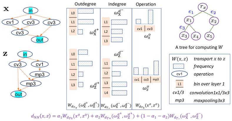
We can leverage the TW distance to compare the $n$-gram representations $\omega_{\mathbf{x}}^{o}$ and $\omega_{\mathbf{z}}^{o}$ using Eq. (2), denoted as $W_{d_{\mathcal{T}_{o}}}\!(\omega_{\mathbf{x}}^{o},\omega_{\mathbf{z}}^{o})$. To compute this distance, we utilize a predefined tree structure for network operations by hierarchically grouping similar network operations into a tree as illustrated in Fig. 1. We can utilize the domain knowledge to define the grouping and the edge weights, such as we can have conv1 and conv3 in the same group and maxpool is from another group. Inspired by the partition-based tree metric sampling (Le et al., 2019b), we define the edge weights decreasing when the edge is far from the root. Although such design can be subjective, the final distance (defined later in Eq. (5)) will be calibrated and normalized properly when modeling with a GP in §3. We refer to Fig. 8 and Appendix §F for the example of TW computation for neural network architectures.

Figure 1: We represent two architectures $\mathbf{x}$ and $\mathbf{z}$ by network structure (via outdegree and indegree) and network operation (using $1$-gram in this example). The similarity between each respective representation is estimated by tree-Wasserstein to compute the minimal cost of transporting one object to another. As a nice property of optimal transport, our tree-Wasserstein can handle different layer sizes and different operation types. The weights in each histogram are calculated from the architectures. The histogram bins in outdegree and indegree are aligned with the network structure in the left. See the Appendix §F for detailed calculations.

$\bullet$ Indegree and outdegree representations for network structure.

We extract the indegree and outdegree of each layer, which are the number of ingoing and outgoing layers respectively, as an alternative way to represent a network structure. We denote $L_{\mathbf{x}}$ as the set of all layers which one can reach from the input layer for neural network $\mathbf{x}$. Let $\eta_{x,\ell}$ and $M_{x}$ be lengths of the longest paths from an input layer to the layer $\ell$ and to the output layer respectively. Such paths interpret the order of layers in a neural network which starts with the input layer, connect with some middle layers, and end with the output layer, we represent the indegree and outdegree of network layers in $\mathbf{x}$ as empirical measures $\omega^{d^{-}}_{\mathbf{x}}$ and $\omega^{d^{+}}_{\mathbf{x}}$, defined as

$$\omega^{d^{-}}_{\mathbf{x}}=\sum_{\ell\in L_{\mathbf{x}}}\mathbf{x}^{d^{-}}_{\ell}\delta_{\frac{\eta_{x,\ell}+1}{M_{x}+1}},\hskip 18.00005pt\omega^{d^{+}}_{\mathbf{x}}=\sum_{\ell\in L_{\mathbf{x}}}\mathbf{x}^{d^{+}}_{\ell}\delta_{\frac{\eta_{x,\ell}+1}{M_{x}+1}},$$ (4)

where $\mathbf{x}^{d^{-}}_{\ell}$ and $\mathbf{x}^{d^{+}}_{\ell}$ are the normalized indegree and outdegree of the layer $\ell$ of $\mathbf{x}$ respectively.

For indegree and outdegree information, the supports of empirical measures $\omega^{d^{-}}_{\mathbf{x}}$, and $\omega^{d^{-}}_{\mathbf{z}}$ are in one-dimensional space that a tree structure reduces to a chain of supports. Thus, we can use $W_{d_{\mathcal{T}_{\!-}}}\!\left(\omega^{d^{-}}_{\mathbf{x}},\omega^{d^{-}}_{\mathbf{z}}\right)$ to compare those empirical measures. Similarly, we have $W_{d_{\mathcal{T}_{\!+}}}\!\left(\omega^{d^{+}}_{\mathbf{x}},\omega^{d^{+}}_{\mathbf{z}}\right)$ for empirical measures $\omega^{d^{+}}_{\mathbf{x}}$ and $\omega^{d^{+}}_{\mathbf{z}}$ built from outdegree information.

Tree-Wasserstein distance for neural networks.

Given neural networks $\mathbf{x}$ and $\mathbf{z}$, we consider three separate TW distances for the $n$-gram, indegree and outdegree representations of the networks respectively. Then, we define $d_{\text{NN}}$ as a convex combination with nonnegative weights $\left\{\alpha_{1},\alpha_{2},\alpha_{3}\mid\sum_{i}\alpha_{i}=1,\alpha_{i}\geq 0\right\}$ for $W_{d_{\mathcal{T}_{o}}}$, $W_{d_{\mathcal{T}_{\!-}}}$, and $W_{d_{\mathcal{T}_{\!+}}}$ respectively, to compare neural networks $\mathbf{x}$ and $\mathbf{z}$ as:

$$d_{\text{NN}}(\mathbf{x},\mathbf{z})=\alpha_{1}W_{d_{\mathcal{T}_{o}}}(\mathbf{x}^{o},\mathbf{z}^{o})+\alpha_{2}W_{d_{\mathcal{T}_{\!-}}}\left(\omega^{d^{-}}_{\mathbf{x}},\omega^{d^{-}}_{\mathbf{z}}\right)\\ +\left(1-\alpha_{1}-\alpha_{2}\right)W_{d_{\mathcal{T}_{\!+}}}\left(\omega^{d^{+}}_{\mathbf{x}},\omega^{d^{+}}_{\mathbf{z}}\right).$$ (5)

The proposed discrepancy $d_{\text{NN}}$ can capture not only the frequency of layer operations, but also network structures, e.g., indegree and outdegree of network layers.

We illustrate our proposed TW for neural networks in Fig. 10 describing each component in Eq. (5). We also describe the detailed calculations in the Appendix §F. We highlight a useful property of our proposed $d_{\text{NN}}$: it can compare two architectures with different layer sizes and/or operations sizes.

Proposition 1.

The $d_{\text{NN}}$ for neural networks is a pseudo-metric and negative definite.

Proof of Proposition 1 is placed in the Appendix §D.2.

Our discrepancy $d_{\text{NN}}$ is negative definite as opposed to the OT for neural networks considered in Kandasamy et al. (2018) which is indefinite. Therefore, from Proposition 1 and following Theorem 3.2.2 in Berg et al. (1984), we can derive a positive definite TW kernel upon $d_{\text{NN}}$ for neural networks $\mathbf{x},\mathbf{z}$ as

$$k(\mathbf{x},\mathbf{z})=\exp\ \bigl{(}-d_{\text{NN}}(\mathbf{x},\mathbf{z})/\sigma^{2}_{l}\bigr{)},$$ (6)

where the scalar $\sigma^{2}_{l}$ is the length-scale parameter. Our kernel has three hyperparameters including a length-scale $\sigma^{2}_{l}$ in Eq. (6); $\alpha_{1}$ and $\alpha_{2}$ in Eq. (5). These hyperparameters will be estimated by maximizing the log marginal likelihood (see Appendix §G). We refer to the Appendix §H for a further discussion about the properties of the pseudo-distance $d_{\text{NN}}$.

3 Neural Architecture Search with Gaussian Process and k-DPP

Problem setting.

We consider a noisy black-box function $f:\mathbb{R}^{d}\rightarrow\mathbb{R}$ over some domain $\mathcal{X}$ containing neural network architectures. As a black-box function, we do not have an explicit formulation for $f$ and it is expensive to evaluate. Our goal is to find the best architecture $\mathbf{x}^{*}\in\mathcal{X}$ such that

$$\mathbf{x}^{*}=\underset{{}_{\mathbf{x}\in\mathcal{X}}}{\text{argmax}}\,f(\mathbf{x}).$$ (7)

We view the black-box function $f$ as a machine learning experiment which takes an input as a neural network architecture $\mathbf{x}$ and produces an accuracy $y$. We can write $y=f(\mathbf{x})+\epsilon$ where we have considered Gaussian noise $\epsilon\sim\mathcal{N}(0,\sigma^{2}_{f})$ given the noise variance $\sigma^{2}_{f}$ estimated from the data.

Bayesian optimization (BO) optimizes the black-box function by sequentially evaluating it (Garnett et al., 2010; Shahriari et al., 2016; Nguyen & Osborne, 2020). Particularly, BO can speed up the optimization process by using a probabilistic model to guide the search (Snoek et al., 2012). BO has demonstrated impressive success for optimizing the expensive black-box functions across domains.

Surrogate models.

Bayesian optimization reasons about $f$ by building a surrogate model, such as a Gaussian process (GP) (Rasmussen, 2006), Bayesian deep learning (Springenberg et al., 2016) or deep neural network (Snoek et al., 2015; White et al., 2021). Among these choices, GP is the most popular model, offering three key benefits: (i) closed-form uncertainty estimation, (ii) evaluation efficiency, and (iii) learning hyperparameters. GP imposes a normally distributed random variable at every point in the input space. The predictive distribution for a new observation also follows a Gaussian distribution (Rasmussen, 2006) where we can estimate the expected function value $\mu(\mathbf{x})$ and the predictive uncertainty $\sigma(\mathbf{x})$ as

$$\mu\left(\mathbf{x}^{\prime}\right) =\mathbf{k}(\mathbf{x}^{\prime},\mathbf{X})\left[\boldsymbol{K}+\sigma^{2}_{f}\mathbf{I}\right]^{-1}\mathbf{y}$$ (8)

$$\sigma^{2}\left(\mathbf{x}^{\prime}\right) =k_{**}-\mathbf{k}(\mathbf{x}^{\prime},\mathbf{X})\left[\boldsymbol{K}+\sigma^{2}_{f}\mathbf{I}\right]^{-1}\mathbf{k}^{T}(\mathbf{x}^{\prime},\mathbf{X})$$ (9)

where $\mathbf{X}=[\mathbf{x}_{1},...\mathbf{x}_{N}]$ and $\mathbf{y}=[y_{1},..y_{N}]$ are the collected architectures and performances respectively; $K(U,V)$ is a covariance matrix whose element $(i,j)$ is calculated as $k(\mathbf{x}_{i},\mathbf{x}_{j})$ with $\mathbf{x}_{i}\in U$ and $\mathbf{x}_{j}\in V$; $k_{**}=k(\mathbf{x}^{\prime},\mathbf{x}^{\prime})$; $\boldsymbol{K}:=\mathbf{K(X,X)}$; $\sigma^{2}_{f}$ is the measurement noise variance and $\mathbf{I}$ is the identity matrix.

Generating a pool of candidates $\mathcal{P}_{t}$.

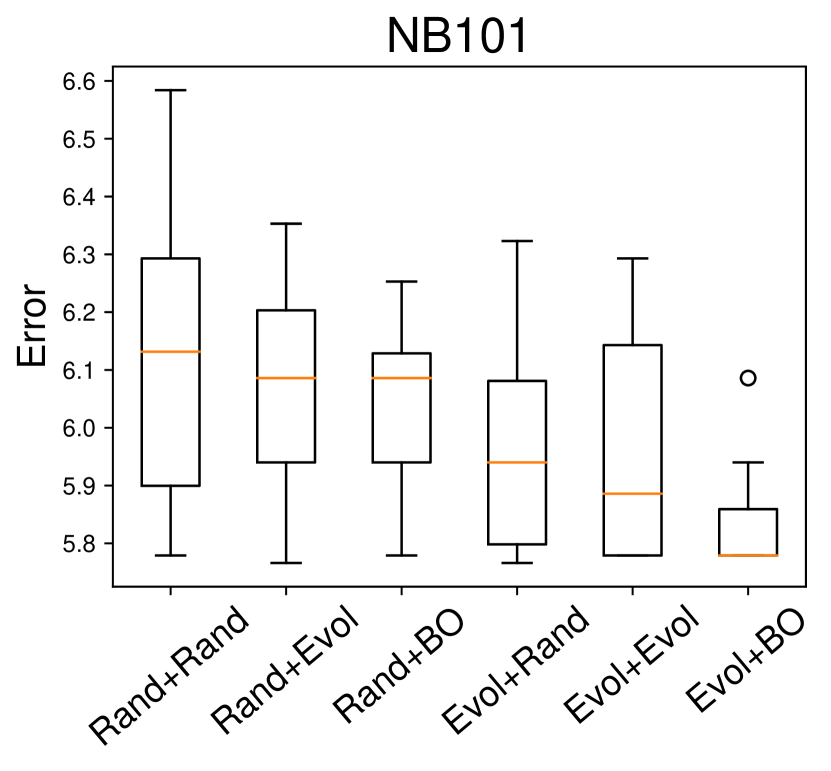
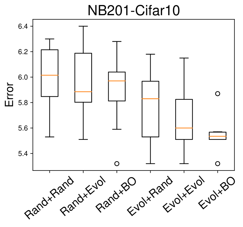
We follow Kandasamy et al. (2018); White et al. (2021) to generate a list of candidate networks using an evolutionary algorithm (Back, 1996). First, we stochastically select top-performing candidates with higher acquisition function values. Then, we apply a mutation operator to each candidate to produce modified architectures. Finally, we evaluate the acquisition given these mutations, add them to the initial pool, and repeat for several steps to get a pool of candidates $\mathcal{P}_{t}$. We design the ablation study in Fig. 2 demonstrating that the evolution strategy outperforms the random strategy for this task.

Optimizing hyperparameters.

We optimize the model hyperparameters by maximizing the log marginal likelihood. We present the derivatives for estimating the hyperparameters $\alpha_{1}$ and $\alpha_{2}$ of the tree-Wasserstein $d_{\text{NN}}$ for neural networks in the Appendix §G. We shall optimize these variables via multi-started gradient descent.

3.1 Sequential NAS using Bayesian optimization

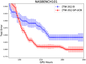
We sequentially suggest a single architecture for evaluation using a decision function $\alpha(\mathbf{x})$ (i.e., acquisition function) from the surrogate model. This acquisition function is carefully designed to trade off between exploration of the search space and exploitation of current promising regions. We utilize the GP-UCB (Srinivas et al., 2010) as the main decision function $\alpha(\mathbf{x})=\mu(\mathbf{x})+\kappa\sigma(\mathbf{x})$ where $\kappa$ is the parameter controlling the exploration, $\mu$ and $\sigma$ are the GP predictive mean and variance in Eqs. (8, 9). Empirically, we find that this GP-UCB generally performs better than expected improvement (EI) (see the Appendix §I.1) and other acquisition functions (see (White et al., 2021)). We note that the GP-UCB also comes with a theoretical guarantee for convergence (Srinivas et al., 2010).

We maximize the acquisition function to select the next architecture $\mathbf{x}_{t+1}=\arg\max_{\mathbf{x}\in\mathcal{P}_{t}}\alpha_{t}\left(\mathbf{x}\right)$. This maximization is done on the discrete set of candidate $\mathcal{P}_{t}$ obtained previously. The selected candidate is the one we expect to be the best if we are optimistic in the presence of uncertainty.

Algorithm 1 Sequential and Parallel NAS using Gaussian process with tree-Wasserstein kernel

1:  Input: Initial data $\mathcal{D}_{0}$, black-box function $f(\mathbf{x})$. Output: The best architecture $\mathbf{x^{*}}$

2:  for $t=1,\ldots,T$ do

3:     Generate architecture candidates $\mathcal{P}_{t}$ by random permutation from the top architectures

4:     Learn a GP (including hyperparameters) using TW from $\mathcal{D}_{t-1}$ to perform estimation over $\mathcal{P}_{t}$ including (i) covariance matrix $K_{\mathcal{P}_{t}}$, (ii) predictive mean $\mu_{\mathcal{P}_{t}}$ and (iii) predictive variance $\sigma_{\mathcal{P}_{t}}$

5:     If Sequential: (i) select a next architecture $\mathbf{x}_{t}=\underset{{}_{\forall\mathbf{x}\in\mathcal{P}_{t}}}{\text{argmax}}\ \alpha(\mathbf{x}\mid\mu_{\mathcal{P}_{t}},\sigma_{\mathcal{P}_{t}})$; then (ii) evaluate the new architecture $y_{t}=f(\mathbf{x}_{t})$; after that, (iii) augment $\mathcal{D}_{t}\leftarrow\mathcal{D}_{t-1}\cup\left(\mathbf{x}_{t},y_{t}\right)$.

6:     If Parallel: (i) select $B$ architectures $\mathbf{X}_{t}=\left[\mathbf{x}_{t,1},,...\mathbf{x}_{t,B}\right]=\text{k-DPP}(\boldsymbol{K}_{\mathcal{P}_{t})}$ in Eq. (12); then (ii) evaluate in parallel $Y_{t}=f(\mathbf{X}_{t})$; after that, (iii) augment $\mathcal{D}_{t}\leftarrow\mathcal{D}_{t-1}\cup\left(\mathbf{X}_{t},Y_{t}\right)$.

7:  end for

3.2 Parallel NAS using Quality k-DPP and GP

The parallel setting speeds up the optimization process by selecting a batch of architectures for parallel evaluations. We present the k-determinantal point process (k-DPP) with quality to select from a discrete pool of candidate $\mathcal{P}_{t}$ for (i) high-performing and (ii) diverse architectures that cover the most information while avoiding redundancy. In addition, diversity is an important property for not being stuck at a local optimal architecture.

The DPP (Kulesza et al., 2012) is an elegant probabilistic measure used to model negative correlations within a subset and hence promote its diversity. A k-determinantal point process (k-DPP) (Kulesza & Taskar, 2011) is a distribution over all subsets of a ground set $\mathcal{P}_{t}$ of cardinality k. It is determined by a positive semidefinite kernel $\boldsymbol{K}_{\mathcal{P}_{t}}$. Let $\boldsymbol{K}_{A}$ be the submatrix of $\boldsymbol{K}_{\mathcal{P}_{t}}$ consisting of the entries $\boldsymbol{K}_{ij}$ with $i,j\in A\subseteq\mathcal{P}_{t}$. Then, the probability of observing $A\subseteq P$ is proportional to $\det(\boldsymbol{K}_{A})$, $\displaystyle P(A\subseteq\mathcal{P}_{t})\propto\det(\boldsymbol{K}_{A}),$ (10) $\displaystyle\boldsymbol{K}_{ij}=q_{i}\phi_{i}^{T}\phi_{j}q_{j}.$ (11)

k-DPP with quality.

While the original idea of the k-DPP is to find a diverse subset, we can extend it to find a subset that is both diverse and high-quality. For this, we write a DPP kernel $k$ as a Gram matrix, $\boldsymbol{K}=\Phi^{T}\Phi$, where the columns of $\Phi$ are vectors representing items in the set $S$. We now take this one step further, writing each column $\Phi$ as the product of a quality term $q_{i}\in\mathcal{R}^{+}$ and a vector of normalized diversity features $\phi_{i}$, $||\phi_{i}||=1$. The entries of the kernel can now be written in Eq. (11).

As discussed in (Kulesza et al., 2012), this decomposition of $\boldsymbol{K}$ has two main advantages. First, it implicitly enforces the constraint that $\boldsymbol{K}$ must be positive semidefinite, which can potentially simplify learning. Second, it allows us to independently model quality and diversity, and then combine them into a unified model. Particularly, we have

$$P_{K}(A)\propto\left(\prod_{i\in A}q_{i}^{2}\right)\det(\phi_{i}^{T}\phi_{i}),$$

where the first term increases with the quality of the selected items, and the second term increases with the diversity of the selected items. Without the quality component, we would get a very diverse set of architectures. However, we might fail to include the most high-performance architectures in $\mathcal{P}_{t}$, focusing instead on low-quality outliers. By integrating the two models, we can achieve a more balanced result.

Figure 2: We study the relative contribution of the strategies generating a pool of candidate $\mathcal{P}$ (Rand and Evolution) versus the main optimization algorithm (Rand, Evolution and BO). The result shows that Evolution can help to improve the performance than Rand in generating a pool of candidate $\mathcal{P}$. Given the same strategy for generating $\mathcal{P}$, BO is significantly better than Rand and Evolution for optimization. Evol+BO is the design in our approach that leads to the best performance.

Conditioning.

In the parallel setting, given the training data, we would like to select high quality and diverse architectures from a pool of candidate $\mathcal{P}_{t}$ described above. We shall condition on the training data in constructing the covariance matrix over the testing candidates from $\mathcal{P}_{t}$. We make the following proposition in connecting the k-DPP conditioning and GP uncertainty estimation. This view allows us to learn the covariance matrix using GP, such as we can maximize the GP marginal likelihood for learning the TW distance and kernel hyperparameters for k-DPP.

Proposition 2.

Conditioned on the training set, the probability of selecting new candidates from a pool $\mathcal{P}_{t}$ is equivalent to the determinant of the Gaussian process predictive covariance matrix.

Proof of Proposition 2 is placed in the Appendix §G.1.

We can utilize the GP predictive mean $\mu(\cdot)$ in Eq. (8) to estimate the quality for any unknown architecture $q_{i}$ defined in Eq. (11). Then, we construct the covariance (kernel) matrix over the test candidates for selection by rewriting Eq. (11) as

$$\boldsymbol{K}_{\mathcal{P}_{t}}\!\left(\mathbf{x}_{i},\mathbf{x}_{j}\right)\!=\!\exp\bigl{(}-\mu(\mathbf{x}_{i})\bigr{)}\sigma(\mathbf{x}_{i},\mathbf{x}_{j})\exp\bigl{(}-\mu(\mathbf{x}_{j})\bigr{)},$$ (12)

for all $\mathbf{x}_{i},\mathbf{x}_{j}\in\mathcal{P}_{t}$ where $\mu(\mathbf{x}_{i})$ and $\sigma(\mathbf{x}_{i},\mathbf{x}_{j})$ are the GP predictive mean and variance defined in Eqs. (8, 9). Finally, we sample $B$ architectures from the covariance matrix $\boldsymbol{K}_{\mathcal{P}_{t}}$ which encodes both the diversity (exploration) and high-utility (exploitation). The sampling algorithm requires precomputing the eigenvalues (Kulesza & Taskar, 2011). Sampling from a k-DPP requires $\mathcal{O}(NB^{2})$ time overall where $B$ is the batch size.

Advantages.

The connection between GP and k-DPP allows us to directly sample diverse and high-quality samples from the GP posterior. This leads to the key advantage that we can optimally sample a batch of candidates without the need of greedy selection. On the other hand, the existing batch BO approaches rely either on greedy strategy (Contal et al., 2013; Desautels et al., 2014; González et al., 2016) to sequentially select the points in a batch or independent sampling (Falkner et al., 2018; Hernández-Lobato et al., 2017). The greedy algorithm is non-optimal and the independent sampling approaches can not fully utilize the information across points in a batch.

We note that our k-DPP above is related to (Kathuria et al., 2016), but different from two perspectives that Kathuria et al. (2016) considers k-DPP for batch BO (i) in the continuous setting and (ii) using pure exploration (without quality). We will consider this as the baseline in our experiments.

4 Experiments

We evaluate our proposed approach on both sequential and parallel neural architecture search (NAS).

Experimental settings. All experimental results are averaged over 30 independent runs with different random seeds. We set the number of candidate architecture $|\mathcal{P}_{t}|=100$. We utilize the popular NAS tabular datasets of Nasbench101 (NB101) (Ying et al., 2019) and Nasbench201 (NB201) (Dong & Yang, 2020) for evaluations. TW and TW-2G stand for our TW using 1-gram and 2-gram representation, respectively. We release the Python code for our experiments at https://github.com/ntienvu/TW_NAS.

4.1 Sequential NAS

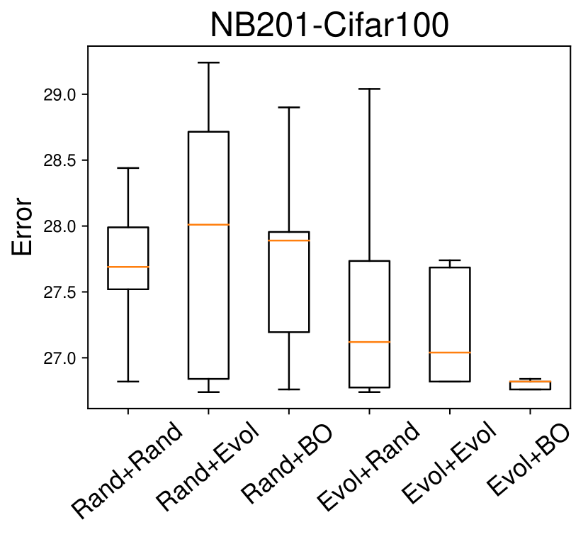
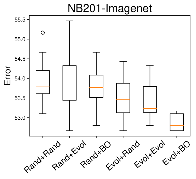
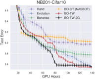
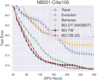
Ablation study: different mechanisms for generating a pool of candidates $\mathcal{P}$. We analyze the relative contribution of the process of generating architecture candidates versus the main optimization algorithm in Fig. 2. The result suggests that the evolutionary algorithm is better than a random strategy to generate a pool of candidates $\mathcal{P}$. Given this generated candidate set $\mathcal{P}$, BO is significantly better than Rand and Evolution approaches. Briefly, the combination of Evol+BO performs the best across datasets.

Figure 3: Sequential NAS on different distances for BO (left) and different baselines (middle and right). Our approaches of BO-TW (black curve) and BO-TW 2G (red curve) for $1$-gram and $2$-gram representation consistently outperform the other baselines. We use $500$ iterations on NB101 and $200$ iterations on NB201.

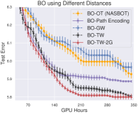
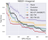
Ablation study: different distances for BO. We design an ablation study using different distances within a BO framework. Notably, we consider the vanilla optimal transport (Wasserstein distance) in which we follow Kandasamy et al. (2018) to define the cost metric for OT. This baseline can be seen as the modified version of the Nasbot (Kandasamy et al., 2018). In addition, we compare our approach with the BO using the Gromov-Wasserstein distance (Mémoli, 2011) (BO-GW) and path encoding (BO-Path Encoding) as used in (White et al., 2021). The results in the left plot of Fig. 3 suggest that the proposed TW using 2-gram performs the best among the BO distance for NAS. The standard OT and GW will result in (non-p.s.d.) indefinite kernels. For using OT and GW in our GP, we keep adding (“jitter”) noise to the diagonal of the kernel matrices until they become p.s.d. kernels. We make use of the POT library (Flamary & Courty, 2017) for the implementation of OT and GW.

While our framework is able to handle $n$-gram representation, we learn that $2$-gram is empirically the best choice. This choice is well supported by the fact that two convolution layers of $3\times 3$ stay together can be used to represent for a special effect of $5\times 5$ convolution kernel. In addition, the use of full $n$-gram may result in very sparse representation and some features are not so meaningful anymore. Therefore, in the experiment we only consider $1$-gram and $2$-gram.

Sequential NAS. We validate our GP-BO model using tree-Wasserstein on the sequential setting. Since NB101 is somewhat harder than NB201, we allocate $500$ queries for NB101 and $200$ queries for NB201 including $10\%$ of random selection at the beginning of BO.

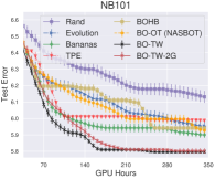
We compare our approach against common baselines including Random search, evolutionary search, TPE (Bergstra et al., 2011), BOHB (Falkner et al., 2018), Nasbot (Kandasamy et al., 2018) and Bananas (White et al., 2021). We use the AutoML library for TPE and BOHB including the results for NB101, but not NB201. We do not compare with Reinforcement Learning approaches (Pham et al., 2018) and AlphaX (Wang et al., 2020) which have been shown to perform poorly in (White et al., 2021).

Figure 4: Estimated hyperparameters on NB101.

We show in Fig. 3 that our tree-Wasserstein including 1-gram and 2-gram will result in the best performance with a wide margin to the second best – the Bananas (White et al., 2021), which needs to specify a meta neural network with extra hyperparameters (layers, nodes, learning rate). Random search performs poorly in NAS due to the high-dimensional and complex space. Our GP-based optimizer offers a closed-form uncertainty estimation without iterative approximation in neural network (via back-propagation). As a property of GP, our BO-TW can generalize well using fewer observations. This can be seen in the right plot of Fig. 3 that our approaches can outperform Bananas when the number of BO iteration (or the number of network architectures for training) is small. On the other hand, both Bananas and ours are converging to the same performance when the training data becomes abundant – but this is not the case in practice for NAS.

Figure 5: Batch NAS comparison using TW-2Gram and a batch size $B=5$. Our proposed k-DPP Quality (red) outperforms other baselines in all cases, especially when the number of training architecture (iterations) is low. This is the desirable property of NAS when the training cost is extremely expensive. The experiments are run over $100$ iterations.

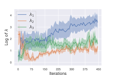
Estimating hyperparameters. We plot the estimated hyperparameters

$$\lambda_{1}=\frac{\alpha_{1}}{\sigma^{2}_{l}},\quad\lambda_{2}=\frac{\alpha_{2}}{\sigma^{2}_{l}},\quad\lambda_{3}=\frac{1-\alpha_{1}-\alpha_{2}}{\sigma^{2}_{l}},$$

over iterations in Fig. 4. This indicates the relative contribution of the operation, indegree and outdegree toward the TW $d_{\text{NN}}$ for neural networks in Eq. (5). Particularly, the operation contributes receives higher weight and is useful information than either the individual indegree or outdegree.

4.2 Parallel NAS

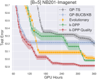
We next demonstrate our model on selecting multiple architectures for parallel evaluation (i.e., parallel NAS) setting. There are fewer approaches for parallel NAS compared to the sequential setting. We select to compare our k-DPP quality against Thompson sampling (Hernández-Lobato et al., 2017), GP-BUCB (Desautels et al., 2014) and k-DPP for batch BO (Kathuria et al., 2016). The GP-BUCB is equivalent to Kriging believer (Ginsbourger et al., 2010) when the hallucinated observation value is set to the GP predictive mean. Therefore, we label them as GP-BUCB/KB. We also compare with the vanilla k-DPP (without using quality) (Kathuria et al., 2016).

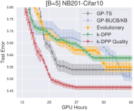
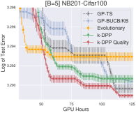
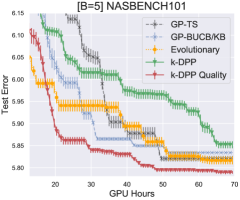
We allocate a maximum budget of $500$ queries including $50$ random initial architectures. The result in Fig. 5 shows that our proposed k-DPP quality is the best among the considered approaches. We refer to the Appendix for additional experiments including varying batch sizes and more results on NB201.

Our sampling from k-DPP quality is advantageous against the existing batch BO approaches (Ginsbourger et al., 2010; Desautels et al., 2014; Kathuria et al., 2016; Hernández-Lobato et al., 2017) in which we can optimally select a batch of architectures without relying on the greedy selection strategy. In addition, our k-DPP quality can leverage the benefit of the GP in estimating the hyperparameters for the covariance matrix.

Figure 6: We compare different batch approaches using a path distance (White et al., 2021) and a batch size $B=5$ . We show that (i) the k-DPP quality outperforms the other batch approaches and (ii) the k-DPP using TW2G (a black curve) performs better than using path distance (a red curve).

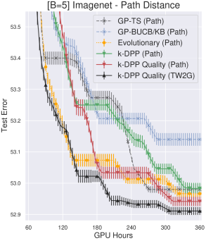
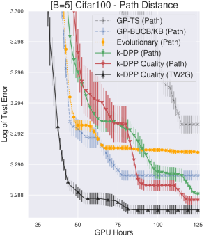
Ablation study of k-DPP quality with path distance. In addition to the proposed tree-Wasserstein, we demonstrate the proposed k-DPP quality using path distance (White et al., 2021). We show that our k-DPP quality is not restricted to TW-2G, but it can be generally used with different choices of kernel distances.

Particularly, we present in Fig. 6 the comparison using two datasets: Imagenet and Cifar100 in NB201. The results validate two following messages. First, our k-DPP quality is the best among the other baselines in selecting high-performing and diverse architectures. Second, our k-DPP quality with TW2G (a black curve) performs better than k-DPP quality using Path distance (a red curve). This demonstrates the key benefits of comparing two complex architectures as logistical supplier and receiver.

5 Conclusion

We have presented a new framework for sequential and parallel NAS. Our proposed framework constructs the similarity between architectures using tree-Wasserstein geometry. Then, it utilizes the Gaussian process surrogate for modeling and optimization. We draw the connection between GP predictive distribution to k-DPP quality for selecting diverse and high-performing architectures from discrete set. We demonstrate our model using Nasbench101 and Nasbench201 that our methods outperform the existing baselines in sequential and parallel settings.

Supplementary Material for: Optimal Transport Kernels for Sequential and Parallel Neural Architecture Search

In this supplementary, we first review the related works in sequential and batch neural architecture search in §A and §B respectively. We next give further detailed information about the datasets in our experiments in §C. Then, we derive detailed proofs for the results in the main text in §D. After that, we give a brief discussion about the tree-Wasserstein geometry in §E, and follow with an example of TW computation for neural network architectures in §F. In §G, we provide additional details of the Bayesian optimization in estimating the hyperparameters. In §H, we show distance properties comparison. Finally, we illustrate further empirical comparisons and analysis for the model in §I.

Appendix A Related works in Neural architecture search

We refer the interested readers to the survey paper (Elsken et al., 2019b) and the literature of neural architecture search for the comprehensive survey on neural architecture search. Many different search strategies have been attempted to explore the space of neural architectures, including random search, evolutionary methods, reinforcement learning (RL), gradient-based methods and Bayesian optimization.

Evolutionary approaches.

Real et al. (2017, 2019); Suganuma et al. (2017); Liu et al. (2018); Shah et al. (2018); Xie & Yuille (2017); Elsken et al. (2019a) have been extensively used for NAS. In the context of evolutionary, the mutation operations include adding a layer, removing a layer or changing the type of a layer (e.g., from convolution to pooling) from the neural network architecture. Then, the evolutionary approaches will update the population, e.g., tournament selection by removing the worst or oldest individual from a population.

Reinforcement learning.

NASNet (Zoph & Le, 2017) is a reinforcement learning algorithm for NAS which achieves state-of-the-art results on CIFAR-10 and PTB; however, the algorithm requires $3000$ GPU days to train. Efficient Neural Architecture Search (ENAS) (Pham et al., 2018) proposes to use a controller that discovers architectures by learning to search for an optimal subgraph within a large graph. The controller is trained with policy gradient to select a subgraph that maximizes the validation set’s expected reward. The model corresponding to the subgraph is trained to minimize a canonical cross-entropy loss. Multiple child models share parameters, ENAS requires fewer GPU-hours than other approaches and $1000$-fold less than "standard" NAS. Other reinforcement learning approaches for NAS have also proposed, such as MetaQNN (Baker et al., 2017) and BlockQNN (Zhong et al., 2018).

Gradient-based approaches.

The works presented in Luo et al. (2018); Liu et al. (2019); Dong & Yang (2019); Yao et al. (2020) represent the search space as a directed acyclic graph (DAG) containing billions of sub-graphs, each of which indicates a kind of neural architecture. To avoid traversing all the possibilities of the sub-graphs, they develop a differentiable sampler over the DAG. The benefit of such an idea is that a differentiable space enables computation of gradient information, which could speed up the convergence of underneath optimization algorithm. Various techniques have been proposed, e.g., DARTS (Liu et al., 2019) , SNAS (Xie et al., 2019) , and NAO (Luo et al., 2018). While these approaches based on gradient-based learning can reduce the computational resources required for NAS, it is currently not well understood if an initial bias in exploring certain parts of the search space more than others might lead to the bias and thus result in premature convergence of NAS (Sciuto et al., 2019). In addition, the gradient-based approach may be less appropriate for exploring different space (e.g., with a completely different number of layers), as opposed to the approach presented in this paper.

Bayesian optimization.

BO has been an emerging technique for black-box optimization when function evaluations are expensive (Rana et al., 2017; Frazier, 2018; Gopakumar et al., 2018; Wan et al., 2021), and it has seen great success in hyperparameter optimization for deep learning (Li & Jamieson, 2018; Nguyen et al., 2020; Ru et al., 2020; Parker-Holder et al., 2020). Recently, Bayesian optimization has been used for searching the best neural architecture (Kandasamy et al., 2018; Jin et al., 2018; White et al., 2021). BO relies on a covariance function to represent the similarity between two data points. For such similarity representation, we can (1) directly measure the similarity of the networks by optimal transport, then modeling with GP surrogate in Kandasamy et al. (2018); or (2) measure the graphs based on the path-based encodings, then modeling with neural network surrogate in White et al. (2021). OTMANN (Kandasamy et al., 2018) shares similarities with Wasserstein (earth mover’s) distances which also have an OT formulation. However, it is not a Wasserstein distance itself—in particular, the supports of the masses and the cost matrices change depending on the two networks being compared. One of the drawback of OTMANN is that it may not be negative definite for a p.s.d. kernel which is an important requirement for modeling with GP. This is the motivation for our proposed tree-Wasserstein.

Path-based encoding. Bananas (White et al., 2021) proposes the path-based encoding for neural network architectures. The drawback of path-based encoding is that we need to enumerate all possible paths from the input node to the output node, in terms of the operations. This can potentially raise although it can work well in NASBench dataset (Ying et al., 2019) which results in $\sum^{5}_{i=0}3^{i}=364$ possible paths.

Kernel graph. Previous work considers the neural network architectures as the graphs, then defining various distances and kernels on graphs (Messmer & Bunke, 1998; Wallis et al., 2001; Kondor & Lafferty, 2002; Smola & Kondor, 2003; Gao et al., 2010; Ru et al., 2021). However, they may not be ideal for our NAS setting because neural networks have additional complex properties in addition to graphical structure, such as the type of operations performed at each layer, the number of neurons, etc. Some methods do allow different vertex sets (Vishwanathan et al., 2010), they cannot handle layer masses and layer similarities.

Appendix B Related works in batch neural architecture search

They are several approaches in the literature which can be used to select multiple architectures for evaluation, including monte carlo tree search (Wang et al., 2020), evolutionary search (Real et al., 2019) and most of the batch Bayesian optimization approaches, such as Krigging believer (Ginsbourger et al., 2010), GP-BUCB (Desautels et al., 2014), B3O (Nguyen et al., 2016), GP-Thompson Sampling (Hernández-Lobato et al., 2017), and BOHB (Falkner et al., 2018).

Krigging believer (KB) (Ginsbourger et al., 2010) exploits an interesting fact about GPs: the predictive variance of GPs depends only on the input $\mathbf{x}$, but not the outcome values $y$. KB will iteratively construct a batch of points. First, it finds the maximum of the acquisition function, like the sequential setting. Next, KB moves to the next maximum by suppressing this point. This is done by inserting the outcome at this point as a halucinated value. This process is repeated until the batch is filled.

GP-BUCB (Desautels et al., 2014) is related to the above Krigging believer in exploiting the GP predictive variance. Particularly, GP-BUCB is similar to KB when the halucinated value is set to the GP predictive mean.

GP-Thompson Sampling (Hernández-Lobato et al., 2017) generates a batch of points by drawing from the posterior distribution of the GP to fill in a batch. In the continuous setting, we can draw a GP sample using random Fourier feature (Rahimi & Recht, 2007). In our discrete case of NAS, we can simply draw samples from the GP predictive mean.

Appendix C Datasets

We summarize two benchmark datasets used in the paper. Neural architecture search (NAS) methods are notoriously difficult to reproduce and compare due to different search spaces, training procedures and computing cost. These make methods inaccessible to most researchers. Therefore, the below two benchmark datasets have been created.

NASBENCH101.

The NAS-Bench-101 dataset contains over $423,000$ neural architectures with precomputed training, validation, and test accuracy (Ying et al., 2019). In NASBench dataset, the neural network architectures have been exhaustively trained and evaluated on CIFAR-10 to create a queryable dataset. Each architecture training takes approximately $0.7$ GPU hour.

NASBENCH201.

NAS-Bench-201 includes all possible architectures generated by $4$ nodes and $5$ associated operation options, which results in $15,625$ neural cell candidates in total. The Nasbench201 dataset includes the tabular results for three subdatasets including CIFAR-10, CIFAR-100 and ImageNet-16-120. Each architecture training for Cifar10 takes approximately $0.7$ GPU hours, Cifar100 takes $1.4$ GPU hours and Imagenet takes $4$ GPU hours.

Appendix D Proofs

D.1 Proof for Lemma 2.1

Proof.

We consider $X\sim GP(m(),k())$. If $k$ is not a p.s.d. kernel, then there is some set of $n$ points $\left(t_{i}\right)_{i=1}^{n}$ and corresponding weights $\alpha_{i}\in\mathcal{R}$ such that

$$\sum_{i=1}^{n}\sum_{j=1}^{n}\alpha_{i}k(t_{i},t_{j})\alpha_{j}<0.$$ (13)

By the GP assumption, $\text{Cov}\bigl{(}X(t_{i}),X(t_{j})\bigr{)}=k(t_{i},t_{j})$, we show that the variance is now negative

$$\text{Var}\left(\sum_{i=1}^{n}\alpha_{i}X(t_{i})\right)=\sum_{i=1}^{n}\sum_{j=1}^{n}\alpha_{i}\text{Cov}\bigl{(}X(t_{i}),X(t_{j})\bigr{)}\alpha_{j}<0.$$ (14)

The negative variance concludes our prove that the GP is no longer valid with non-p.s.d. kernel.

∎

D.2 Proof for Proposition 1

Proof.

We have that tree-Wasserstein (TW) is a metric and negative definite (Le et al., 2019b). Therefore, $W_{d_{\mathcal{T}_{o}}},W_{d_{\mathcal{T}_{\!-}}},W_{d_{\mathcal{T}_{\!+}}}$ are also a metric and negative definite.

Moreover, the discrepancy $d_{\text{NN}}$ is a convex combination with positive weights for $W_{d_{\mathcal{T}_{o}}},W_{d_{\mathcal{T}_{\!-}}},W_{d_{\mathcal{T}_{\!+}}}$. Therefore, it is easy to verify that for given neural networks $\mathbf{x}_{1},\mathbf{x}_{2},\mathbf{x}_{3}$, we have:

• $d_{\text{NN}}(\mathbf{x}_{1},\mathbf{x}_{1})=0$,

• $d_{\text{NN}}(\mathbf{x}_{1},\mathbf{x}_{2})=d_{\text{NN}}(\mathbf{x}_{2},\mathbf{x}_{1})$,

• $d_{\text{NN}}(\mathbf{x}_{1},\mathbf{x}_{2})+d_{\text{NN}}(\mathbf{x}_{1},\mathbf{x}_{2})\geq d_{\text{NN}}(\mathbf{x}_{2},\mathbf{x}_{3})$.

Thus, $d_{\text{NN}}$ is a pseudo-metric. Additionally, a convex combination with positive weights preserves the negative definiteness. Therefore, $d_{\text{NN}}$ is negative definite. ∎

D.3 Tree-Wasserstein kernel for neural networks

Proposition 3.

Given the scalar length-scale parameter $\sigma^{2}_{l}$, the tree-Wasserstein kernel for neural networks $k(x,z)=\exp(-\frac{d_{\text{NN}}(x,z)}{\sigma^{2}_{l}})$ is infinitely divisible.

Proof.

Given two neural networks $\mathbf{x}$ and $\mathbf{z}$, we introduce new kernels $k_{\gamma}(\mathbf{x},\mathbf{z})=\exp\bigl{(}-\frac{d_{\text{NN}}(\mathbf{x},\mathbf{z})}{\gamma\sigma^{2}_{l}}\bigr{)}$ for $\gamma\in\mathbb{N}^{*}$. Following Berg et al. (1984) (Theorem 3.2.2, p.74), $k_{\gamma}(x,z)$ is also positive definite. Moreover, we also have $k(\mathbf{x},\mathbf{z})=\bigl{(}k_{\gamma}(\mathbf{x},\mathbf{z})\bigr{)}^{\gamma}$. Then, following Berg et al. (1984) (Definition 2.6, p.76), we complete the proof. ∎

From Proposition 3, one does not need to recompute the Gram matrix of the TW kernel for each choice of $\sigma^{2}_{l}$, since it suffices to compute it once.

Appendix E A brief discussion on tree-Wasserstein geometry

Tree-Wasserstein is a special case of the optimal transport (OT) where the ground cost is the tree metric (Do Ba et al., 2011; Le et al., 2019b). Tree-(sliced)-Wasserstein is a generalized version of the sliced-Wassersttein (SW) which projects supports into a line (i.e., one dimensional space) and relies on the closed-form solution of the univariate OT. Moreover, the tree-Wasserstein alleviates the curse of dimensionality for the sliced-Wasserstein. Moreover, the tree-Wasserstein has a closed-form for computation and is negative definite which supports to build positive definite kernels.

The tree structure has been leveraged for various optimal transport problems, especially for large-scale settings such as the unbalanced OT problem where distributions have different total mass (Le & Nguyen, 2021), the Gromov-Wasserstein problem where supports of distributions are in different spaces (Le et al., 2021; Mémoli et al., 2021), Gromov-Hausdoff problem for metric measure spaces (Mémoli et al., 2019), or the Wasserstein barycenter problem which finds the closest distribution to a given set of distributions (Le et al., 2019a).

In our work, we propose tree-Wasserstein for neural network architectures by leveraging a novel design of tree structures on network operations, indegree and outdegree representation for network structure. Therefore, our tree-Wasserstein for neural network can capture not only the frequency of layer operations (i.e., $n$-gram representation for layer operations) but also the entire network structure (i.e., indegree and outdegree representation).

Appendix F An example of TW computation for neural network architectures

We would like to recall the TW distance between probability measures in Equation (2):

$$W_{d_{\mathcal{T}}}(\omega,\nu)=\sum_{e\in\mathcal{T}}w_{e}\bigl{|}\omega\bigl{(}\Gamma(v_{e})\bigr{)}-\nu\bigl{(}\Gamma(v_{e})\bigr{)}\bigr{|}.$$ (15)

We emphasize that tree Wasserstein (TW) is computed as a sum over edges in a tree, but not the sum over supports (e.g., in $1$-gram representation). We next explain all components in TW (Equation (2)) for computation in details.

Figure 7: We illustrate a tree metric using a tree $\mathcal{T}$ which is used to explain the TW formula in Eq. (2). See text for more details.

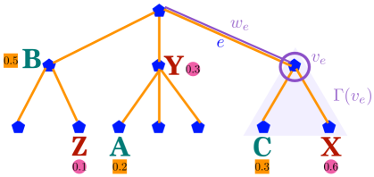
Let consider the tree metric illustrated in Fig. 7, and two probability measures $\omega=0.2\delta_{A}+0.5\delta_{B}+0.3\delta_{C}$, and $\nu=0.6\delta_{X}+0.3\delta_{Y}+0.1\delta_{Z}$. In this example, $A,B,C$ are supports of probability measure $\omega$ with corresponding weights $0.2,0.5,0.3$. In other words, the mass of the probability measure $\omega$ at each support $A,B,C$ is $0.2,0.5,0.3$ respectively. Similarly, $X,Y,Z$ are supports of probability measure $\nu$ with corresponding weights $0.6,0.3,0.1$. Next, let consider edge $e$ in Fig. 7 (the blue $e$), we have the following:

• $w_{e}$ is the weight (or length) of the edge $e$ (the purple line to emphasize the edge blue $e$);

• $v_{e}$ is one of the two nodes of the edge $e$ which is farther away from the tree root (the node with the purple circle);

• $\Gamma(v_{e})$ is the subtree rooted at $v_{e}$ (illustrated by the purple triangle blurred region);

• For the probability measure $\omega$: $\omega\bigl{(}\Gamma(v_{e})\bigr{)}$ is the total mass of the probability measure $\omega$ in the subtree $\Gamma(v_{e})$; and only the support $C$ (with weight $0.3$) of $\omega$ is on the subtree $\Gamma(v_{e})$. Hence, $\omega(\Gamma(v_{e}))=0.3$.

• For the probability measure $\nu$: $\nu\bigl{(}\Gamma(v_{e})\bigr{)}=0.6$. There is only the support $X$ with weight $0.6$ of $\nu$ is in the subtree $\Gamma(v_{e})$.

We do the same procedure for all other edges in the tree $\mathcal{T}$ for the TW computation.

Intuitively, in case we consider the map $g:\omega\mapsto w_{e}\omega\bigl{(}\Gamma(e)\bigr{)}\mid_{e\in\mathcal{T}}$, we have $g(\omega)\in\mathbb{R}^{m}$ where $m$ is the number of edges in the tree $\mathcal{T}$. The TW distance between two probability measures $\omega,\nu$ is equivalent to the $\ell_{1}$ distance between two $m$-dimensional (non-negative) vectors $g(\omega),g(\nu)$.

Now, we are ready to present an example of using TW for transporting two neural network architectures in Fig. 8. We consider a set $\SS$ of interest operations as follow $\SS=\left\{\texttt{cv1, cv3, mp3}\right\}$.

Figure 8: Example of TW used for calculating two architectures. The label of each histogram bin is highlighted in green. The distance between two nodes in a tree is sum of total cost if we travel between the two nodes, see Eq. (2). For example, the cost for moving maxpool ($m$) to conv1 ($c1$) is $1+0.9+0.1=2$. We use similar analogy for computing in 2-gram (2g) representation. For the tree construction, let consider the the $1$-gram tree, we group c1 (conv1) and c3 (conv3) due to their similarity, and "c" (conv) is an abstract label for the group of "convolution". We define the edge weights decreasing when the edge is far from the root, inspired by the partition-based tree metric sampling method (see the "$n$-gram representation for layer operations" part in $\S$2.2).

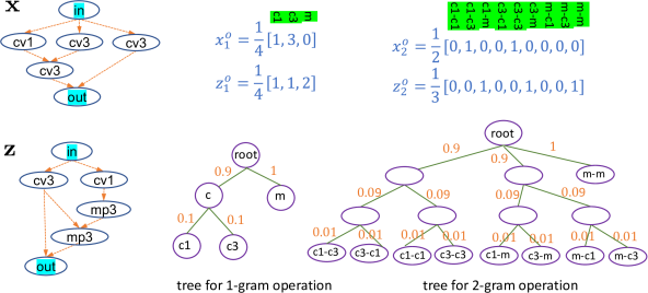
Neural network information $\left(\mathcal{S}^{o},A\right)$.

We use the order top-bottom and left-right for layers in $\mathcal{S}^{o}$.

• For neural network $\mathbf{x}$, we have $\mathcal{S}^{o}_{\mathbf{x}}=\left\{\texttt{in, cv1, cv3, cv3, cv3, out}\right\}$,

  $$A_{\mathbf{x}}=\begin{pmatrix}0&1&1&1&0&0\\ 0&0&0&0&1&0\\ 0&0&0&0&1&0\\ 0&0&0&0&0&1\\ 0&0&0&0&0&1\\ 0&0&0&0&0&0\end{pmatrix}$$

• For neural network $\mathbf{z}$, we have $\mathcal{S}^{o}_{\mathbf{z}}=\left\{\texttt{in, cv3, cv1, mp3, mp3, out}\right\},$

  $$A_{\mathbf{z}}=\begin{pmatrix}0&1&1&0&0&0\\ 0&0&0&0&1&1\\ 0&0&0&1&0&0\\ 0&0&0&0&1&0\\ 0&0&0&0&0&1\\ 0&0&0&0&0&0\end{pmatrix}$$

We show how to calculate these three representations (layer operation, indegree and outdegree) using tree-Wasserstein.

F.1 $n$-gram representation for layer operations

$\bullet$ $1$-gram representation.

The $1$-gram representations $\mathbf{x}^{o}_{1}$ and $\mathbf{z}^{o}_{1}$ for neural network $\mathbf{x}$, and $\mathbf{z}$ respectively are:

$$\mathbf{x}^{o}_{1}=\frac{1}{4}(1,3,0)\qquad\mathbf{z}^{o}_{1}=\frac{1}{4}(1,1,2)$$

where we use the order (1:cv1, 2:cv3, 3:mp3) for the frequency of interest operations in the set $\SS$ for the $1$-gram representation of neural network.

$\bullet$ $2$-gram representation.

For the $2$-gram representations $\mathbf{x}^{o}_{2}$ and $\mathbf{z}^{o}_{2}$ for neural networks $\mathbf{x}$ and $\mathbf{z}$ respectively, we use the following order for $\SS\times\SS$: (1:cv1-cv1, 2:cv1-cv3, 3:cv1-mp3, 4:cv3-cv1, 5:cv3-cv3, 6:cv3:mp3, 7:mp3-cv1, 8:mp3:cv3, 9:mp3-mp3). Thus, we have

$$\mathbf{x}^{o}_{2}=\frac{1}{2}(0,1,0,0,1,0,0,0,0),\qquad\mathbf{z}^{o}_{2}=\frac{1}{3}(0,0,1,0,0,1,0,0,1).$$

Or, we can represent them as empirical measures

$$\omega_{\mathbf{x}^{o}_{2}}=\frac{1}{2}\delta_{\texttt{cv1-cv3}}+\frac{1}{2}\delta_{\texttt{cv3-cv3}},\hskip 47.0pt\qquad \omega_{\mathbf{z}^{o}_{2}}=\frac{1}{3}\delta_{\texttt{cv1-mp3}}+\frac{1}{3}\delta_{\texttt{cv3-mp3}}+\frac{1}{3}\delta_{\texttt{mp3-mp3}}.$$

$\bullet$ Tree metrics for $n$-gram representations for layer operations.

We can use the tree metric in Fig. 8 for $1$-gram and $2$-gram representations. The tree metric for operations are summarized in Table 1.

Table 1: The tree-metric for operations in $W_{d_{\mathcal{T}_{o}}}$ from our predefined tree in Fig. 8 satisfying the following properties: (i) identical operation (cv1,cv1) has zero cost, (ii) similar operations (cv1,cv3) have small cost, and (iii) very different operations (cv1,mp3) have high cost. Then, the similarity score is normalized in Eq. (5) and Eq. (6) in which the weighting parameters $\alpha$ are learnt directly from the data. The utility score is further standardized $\mathcal{N}(0,1)$ for robustness. Therefore, our model is robust to the choice of the predefined tree for the cost in this table. (Recall that the cost in the table is computed by tree metric (i.e., the length of the shortest path) between the pair-wise operations in the predefined tree in Fig. 8.)

	cv1	cv3	mp3
cv1	$0$	$0.2$	$2$
cv3	$0.2$	$0$	$2$
mp3	$2$	$2$	$0$

Using the closed-form computation of tree-Wasserstein presented in Eq. (2) in the main text, we can compute $W_{d_{\mathcal{T}_{o}}}(\mathbf{x}^{o}_{1},\mathbf{z}^{o}_{1})$ for $1$-gram representation and $W_{d_{\mathcal{T}_{o}}}(\mathbf{x}^{o}_{2},\mathbf{z}^{o}_{2})$ for $2$-gram representation.

For $1$-gram representation, we have

$$W_{d_{\mathcal{T}_{o}}}(\mathbf{x}^{o}_{1},\mathbf{z}^{o}_{1})=0.1\left|\frac{1}{4}-\frac{1}{4}\right|+0.1\left|\frac{3}{4}-\frac{1}{4}\right|+0.9\left|1-\frac{2}{4}\right|+1\left|0-\frac{2}{4}\right|=1.$$ (16)

For $2$-gram representation, we have

$$W_{d_{\mathcal{T}_{o}}}(\mathbf{x}^{o}_{2},\mathbf{z}^{o}_{2})= 0.1\left|\frac{1}{2}-0\right|+0.1\left|\frac{1}{2}-0\right|+0.9\left|1-0\right|$$ (17)

$$+0.01\left|0-\frac{1}{3}\right|+0.01\left|0-\frac{1}{3}\right|+0.99\left|0-\frac{2}{3}\right|+1\left|0-\frac{1}{3}\right|=2.$$

F.2 Indegree and outdegree representations for network structure

The indegree and outdegree empirical measures $(\omega^{d^{-}}_{\mathbf{x}},\omega^{d^{+}}_{\mathbf{x}})$ and $(\omega^{d^{-}}_{\mathbf{z}},\omega^{d^{+}}_{\mathbf{z}})$ for neural networks $\mathbf{x}$ and $\mathbf{z}$ respectively are:

$$\omega^{d^{-}}_{\mathbf{x}}=\sum_{i=1}^{6}\mathbf{x}^{d^{-}}_{i}\delta_{\frac{\eta_{\mathbf{x},i}+1}{M_{\mathbf{x}}+1}},\qquad\omega^{d^{+}}_{\mathbf{x}}=\sum_{i=1}^{6}\mathbf{x}^{d^{+}}_{i}\delta_{\frac{\eta_{\mathbf{x},i}+1}{M_{\mathbf{x}}+1}}$$ (18)

$$\omega^{d^{-}}_{\mathbf{z}}=\sum_{i=1}^{6}\mathbf{z}^{d^{-}}_{i}\delta_{\frac{\eta_{\mathbf{z},i}+1}{M_{\mathbf{z}}+1}},\qquad\omega^{d^{+}}_{\mathbf{z}}=\sum_{i=1}^{6}\mathbf{z}^{d^{+}}_{i}\delta_{\frac{\eta_{\mathbf{z},i}+1}{M_{\mathbf{z}}+1}},$$ (19)

where

$$\mathbf{x}^{d^{-}}=\left(0,\frac{1}{7},\frac{1}{7},\frac{1}{7},\frac{2}{7},\frac{2}{7}\right),\qquad\mathbf{x}^{d^{+}}=\left(\frac{3}{7},\frac{1}{7},\frac{1}{7},\frac{1}{7},\frac{1}{7},0\right),$$ (20)

$$\mathbf{z}^{d^{-}}=\left(0,\frac{1}{7},\frac{1}{7},\frac{1}{7},\frac{2}{7},\frac{2}{7}\right),\qquad\mathbf{z}^{d^{+}}=\left(\frac{2}{7},\frac{2}{7},\frac{1}{7},\frac{1}{7},\frac{1}{7},0\right),$$ (21)

$$\eta_{\mathbf{x}}=\left(0,1,1,1,2,3\right),\qquad\qquad\eta_{\mathbf{z}}=\left(0,1,1,2,3,4\right),$$ (22)

$M_{\mathbf{x}}=3$, $M_{\mathbf{z}}=4$, and $\mathbf{x}^{d^{-}}_{i},\mathbf{x}^{d^{+}}_{i},\eta_{\mathbf{x},i}$ are the $i^{th}$ elements of $\mathbf{x}^{d^{-}},\mathbf{x}^{d^{+}},\eta_{\mathbf{x}}$ respectively. Consequently, one can leverage the indegree and outdegree for network structures to distinguish between $\mathbf{x}$ and $\mathbf{z}$.

We demonstrate in Fig. 9 how to calculate the tree-Wasserstein for indegree and outdegree. The supports of empirical measures $\omega^{d^{-}}_{\mathbf{x}}$ and $\omega^{d^{-}}_{\mathbf{z}}$ are in a line. For simplicity, we choose a tree as a chain of real values for the tree-Wasserstein distance. The tree becomes a chain of increasing real values, i.e., $\frac{1}{4}\rightarrow\frac{2}{4}\rightarrow\frac{3}{4}\rightarrow 1$, the weight in each edge is the $\ell_{1}$ distance between two nodes of that edge. Particularly, the tree-Wasserstein is equivalent to the univariate optimal transport. It is similar for empirical measures $\omega^{d^{+}}_{\mathbf{x}}$ and $\omega^{d^{+}}_{\mathbf{z}}$.

Figure 9: Illustration of indegree and outdegree used in TW. Let $\eta_{x,\ell}$ and $M_{x}$ be lengths of the longest paths from an input layer to a layer $\ell$ and to an output layer respectively. We can represent the empirical measure as $\omega^{d^{-}}_{\mathbf{x}}=\sum_{\ell\in L_{\mathbf{x}}}\mathbf{x}^{d^{-}}_{\ell}\delta_{\frac{\eta_{x,\ell}+1}{M_{x}+1}}=\frac{3}{7}\delta_{\frac{2}{4}}+\frac{2}{7}\delta_{\frac{3}{4}}+\frac{2}{7}\delta_{\frac{4}{4}}$ and $\omega^{d^{+}}_{\mathbf{x}}=\sum_{\ell\in L_{\mathbf{x}}}\mathbf{x}^{d^{+}}_{\ell}\delta_{\frac{\eta_{x,\ell}+1}{M_{x}+1}}=\frac{3}{7}\delta_{\frac{1}{4}}+\frac{3}{7}\delta_{\frac{2}{4}}+\frac{1}{7}\delta_{\frac{3}{4}}$ and for $\mathbf{z}$ as $\omega^{d^{-}}_{\mathbf{z}}=\sum_{\ell\in L_{\mathbf{z}}}\mathbf{z}^{d^{-}}_{\ell}\delta_{\frac{\eta_{z,\ell}+1}{M_{z}+1}}=\frac{2}{7}\delta_{\frac{2}{5}}+\frac{1}{7}\delta_{\frac{3}{5}}+\frac{2}{7}\delta_{\frac{4}{5}}+\frac{2}{7}\delta_{\frac{5}{5}}$ and $\omega^{d^{+}}_{\mathbf{x}}=\sum_{\ell\in L_{\mathbf{z}}}\mathbf{z}^{d^{+}}_{\ell}\delta_{\frac{\eta_{z,\ell}+1}{M_{z}+1}}=\frac{2}{7}\delta_{\frac{1}{5}}+\frac{3}{7}\delta_{\frac{2}{5}}+\frac{1}{7}\delta_{\frac{3}{5}}+\frac{1}{7}\delta_{\frac{4}{5}}$. The tree, which is a chain (1/5 $\rightarrow$ 1/4 $\rightarrow$ 2/5 $\rightarrow$ 2/4 $\rightarrow$ 3/5 $\rightarrow$ 3/4 $\rightarrow$ 4/5 $\rightarrow$ 1), is used to compute the distance.

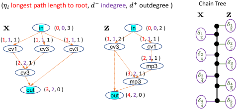
$\bullet$ $W_{d_{\mathcal{T}_{\!-}}}(\omega_{\mathbf{x}}^{d^{-}},\omega_{\mathbf{z}}^{d^{-}})$ for indegree representation.

Using Eq. (2) we have

$$W_{d_{\mathcal{T}_{\!-}}}(\omega_{\mathbf{x}}^{d^{-}},\omega_{\mathbf{z}}^{d^{-}}) =\left(\frac{1}{4}-\frac{1}{5}\right)\underbrace{\left|\frac{7}{7}-\frac{7}{7}\right|}_{\Gamma\left(\delta_{\frac{1}{4}}\right)}+\left(\frac{2}{5}-\frac{1}{4}\right)\underbrace{\left|\frac{7}{7}-\frac{7}{7}\right|}_{\Gamma\left(\delta_{\frac{2}{5}}\right)}+\left(\frac{2}{4}-\frac{2}{5}\right)\underbrace{\left|\frac{7}{7}-\frac{5}{7}\right|}_{\Gamma\left(\delta_{\frac{2}{4}}\right)}+\left(\frac{3}{5}-\frac{2}{4}\right)\underbrace{\left|\frac{4}{7}-\frac{5}{7}\right|}_{\Gamma\left(\delta_{\frac{3}{5}}\right)}$$ (23)

$$+\left(\frac{3}{5}-\frac{2}{4}\right)\underbrace{\left|\frac{4}{7}-\frac{4}{7}\right|}_{\Gamma\left(\delta_{\frac{3}{4}}\right)}+\left(\frac{3}{5}-\frac{2}{4}\right)\underbrace{\left|\frac{2}{7}-\frac{4}{7}\right|}_{\Gamma\left(\delta_{\frac{4}{5}}\right)}+\left(\frac{3}{5}-\frac{2}{4}\right)\underbrace{\left|\frac{2}{7}-\frac{2}{7}\right|}_{\Gamma\left(\delta_{1}\right)}=\frac{4}{70}=0.0571$$

where for each value $\left(t_{1}-t_{2}\right)\left|a_{1}-a_{2}\right|$, the value in the parenthesis, e.g., $\left(t_{1}-t_{2}\right)$, is defined as the edge weights from $\delta_{t_{1}}$ to $\delta_{t_{2}}$ in Fig. 9 and the values in the absolute difference, e.g., $\left|a_{1}-a_{2}\right|$ is the total mass of empirical measures in the subtrees rooted as the deeper node (i.e., $\delta_{t_{2}}$) of corresponding edge (from $\delta_{t_{1}}$ to $\delta_{t_{2}}$) as defined in Eq. (2).

$\bullet$ $W_{d_{\mathcal{T}_{\!+}}}(\omega_{\mathbf{x}}^{d^{+}},\omega_{\mathbf{z}}^{d^{+}})$ for outdegree representation.

Similarly, for outdegree representation, we have

$$W_{d_{\mathcal{T}_{\!+}}}(\omega_{\mathbf{x}}^{d^{+}},\omega_{\mathbf{z}}^{d^{+}}) =\left(\frac{1}{4}-\frac{1}{5}\right)\underbrace{\left|\frac{7}{7}-\frac{5}{7}\right|}_{\Gamma\left(\delta_{\frac{1}{4}}\right)}+\left(\frac{2}{5}-\frac{1}{4}\right)\underbrace{\left|\frac{4}{7}-\frac{5}{7}\right|}_{\Gamma\left(\delta_{\frac{2}{5}}\right)}+\left(\frac{2}{4}-\frac{2}{5}\right)\underbrace{\left|\frac{4}{7}-\frac{2}{7}\right|}_{\Gamma\left(\delta_{\frac{2}{4}}\right)}+\left(\frac{3}{5}-\frac{2}{4}\right)\underbrace{\left|\frac{1}{7}-\frac{2}{7}\right|}_{\Gamma\left(\delta_{\frac{3}{5}}\right)}$$ (24)

$$+\left(\frac{3}{5}-\frac{2}{4}\right)\underbrace{\left|\frac{1}{7}-\frac{1}{7}\right|}_{\Gamma\left(\delta_{\frac{3}{4}}\right)}+\left(\frac{3}{5}-\frac{2}{4}\right)\underbrace{\left|\frac{0}{7}-\frac{1}{7}\right|}_{\Gamma\left(\delta_{\frac{4}{5}}\right)}+\left(\frac{3}{5}-\frac{2}{4}\right)\underbrace{\left|\frac{0}{7}-\frac{0}{7}\right|}_{\Gamma\left(\delta_{1}\right)}=\frac{6}{70}=0.0857.$$

From $W_{d_{\mathcal{T}_{o}}}$, $W_{d_{\mathcal{T}_{\!-}}}$ and $W_{d_{\mathcal{T}_{\!+}}}$, we can obtain the discrepancy $d_{\text{NN}}$ between neural networks $\mathbf{x}$ and $\mathbf{z}$ as in Eq. (5) with predefined values $\alpha_{1},\alpha_{2},\alpha_{3}$.

Appendix G Optimizing hyperparameters in TW and GP

As equivalence, we consider $\lambda_{1}=\frac{\alpha_{1}}{\sigma^{2}_{l}}$, $\lambda_{2}=\frac{\alpha_{2}}{\sigma^{2}_{l}}$ and $\lambda_{3}=\frac{1-\alpha_{1}-\alpha_{2}}{\sigma^{2}_{l}}$ in Eq. (6) and present the derivative for estimating the variable $\lambda$ in our kernel.

$$k(\mathbf{u},\mathbf{v})=\exp\left(-\lambda_{1}W_{d_{\mathcal{T}_{o}}}(\mathbf{u},\mathbf{v})-\lambda_{2}W_{d_{\mathcal{T}_{\!-}}}(\mathbf{u},\mathbf{v})-\lambda_{3}W_{d_{\mathcal{T}_{\!+}}}(\mathbf{u},\mathbf{v})\right).$$ (25)

The hyperparameters of the kernel are optimised by maximising the log marginal likelihood (LML) of the GP surrogate

$$\theta^{*}=\arg\max_{\theta}\mathcal{L}(\theta,\mathcal{D}),$$ (26)

where we collected the hyperparameters into $\theta=\{\lambda_{1},\lambda_{2},\lambda_{3},\sigma^{2}_{n}\}$. The LML (Rasmussen, 2006) and its derivative are defined as

$$\mathcal{L}(\theta)=-\frac{1}{2}\mathbf{y}^{\intercal}\mathbf{K}^{-1}\mathbf{y}-\frac{1}{2}\log|\mathbf{K}|+\text{constant}$$ (27)

$$\frac{\partial\mathcal{L}}{\partial\theta}=\frac{1}{2}\left(\mathbf{y}^{\intercal}\mathbf{K}^{-1}\frac{\partial\mathbf{K}}{\partial\theta}\mathbf{K}^{-1}\mathbf{y}-\text{tr}\left(\mathbf{K}^{-1}\frac{\partial\mathbf{K}}{\partial\theta}\right)\right),$$ (28)

where $\mathbf{y}$ are the function values at sample locations and $\mathbf{K}$ is the covariance matrix of $k(\mathbf{x},\mathbf{x}^{\prime})$ evaluated on the training data. Optimization of the LML was performed via multi-started gradient descent. The gradient in Eq. (28) relies on the gradient of the kernel $k$ w.r.t. each of its parameters:

$$\frac{\partial k(\mathbf{u},\mathbf{v})}{\partial\lambda_{1}} =-W_{d_{\mathcal{T}_{o}}}(\mathbf{u},\mathbf{v})\times k(\mathbf{u},\mathbf{v})$$ (29)

$$\frac{\partial k(\mathbf{u},\mathbf{v})}{\partial\lambda_{2}} =-W_{d_{\mathcal{T}_{\!-}}}(\mathbf{u},\mathbf{v})\times k(\mathbf{u},\mathbf{v})$$ (30)

$$\frac{\partial k(\mathbf{u},\mathbf{v})}{\partial\lambda_{3}} =-W_{d_{\mathcal{T}_{\!+}}}(\mathbf{u},\mathbf{v})\times k(\mathbf{u},\mathbf{v}).$$ (31)

G.1 Proof for Proposition 2

Proof.

Let $A$ and $B$ be the training and test set respectively, we utilize the Schur complement to have $K_{A\cup B}=K_{A}\times\left[K_{B}-K_{BA}K_{A}^{-1}K_{AB}\right]$ and the probability of selecting $B$ is

$$P\left(B\subset\mathcal{P}\mid A\right)=\frac{\det\left(K_{A\cup B}\right)}{\det(K_{A})}=\det\left(K_{B}-K_{BA}K_{A}^{-1}K_{AB}\right)=\det\left(\sigma(B\mid A)\right).$$ (32)

This shows that the conditioning of k-DPP is equivalent to the GP predictive variance $\sigma(B\mid A)$ in Eq. (9).

∎

Appendix H Distance Properties Comparison

We summarize the key benefits of using tree-Wasserstein (n-gram) as the main distance with GP for sequential NAS and k-DPP for batch NAS in Table 2. Tree-Wasserstein offers close-form computation and positive semi-definite covariance matrix which is critical for GP and k-DPP modeling.

Comparison with graph kernel.

Besides the adjacency matrix representation, each architecture includes layer masses and operation type. We note that two different architectures may share the same adjacency matrix while they are different in operation type and layer mass.

Comparison with path-based encoding.

TW can scale well to more nodes, layers while the path-based encoding is limited to.

Comparison with OT approaches in computational complexity.

In general, OT is formulated as a linear programming problem and its computational complexity is super cubic in the size of probability measures (Burkard & Cela, 1999) (e.g., using network simplex). On the other hand, TW has a closed-form computation in Eq. (2), and its computational complexity is linear to the number of edges in the tree. Therefore, TW is much faster than OT in applications (Le et al., 2019b), and especially useful for large-scale settings where the computation of OT becomes prohibited.

Table 2: Properties comparison across different distances for using with GP-BO and k-DPP. GW is Gromov-Wasserstein. TW is tree-Wasserstein. OT is optimal transport.

Representation	Matrix/Graph	Path-Encoding	OT (or W)	GW	TW
Closed-form estimation	✓	✓	✗	✗	✓
Positive semi definite	✓	✓	✗	✗	✓
Different architecture sizes	✓, ✗	✗	✓	✓	✓
Scaling with architecture size	✓	✗	✓	✓	✓

Figure 10: Tree-Wasserstein distances over 500 architectures on NASBENCH101.

Figure 11: Additional sequential NAS comparison on NASBENCH201.

Appendix I Additional Experiments and Illustrations

I.1 Model Analysis

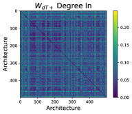
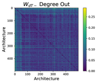
We illustrate three internal distances of our tree-Wasserstein including $W_{d_{\mathcal{T}_{o}}}$, $W_{d_{\mathcal{T}_{\!+}}}$, $W_{d_{\mathcal{T}_{\!-}}}$ in Fig. 10. Each internal distance captures different aspects of the networks. The zero diagonal matrix indicates the correct estimation of the same neural architectures.

Figure 12: Additional result of batch NAS on NB101. We use TW-2G and a batch size $B=5$

I.2 Further sequential and batch NAS experiments

To complement the results presented in the main paper, we present additional experiments on both sequential and batch NAS setting using NB101 and NB201 dataset in Fig. 11. In addition, we present experiments on batch NAS settings in Fig. 12 that the proposed k-DPP quality achieves the best performance consistently.

I.3 Ablation study using different acquisition functions

We evaluate our proposed model using two comon acquisition functions including UCB and EI. The result suggests that UCB tends to perform much better than EI for our NAS setting. This result is consistent with the comparison presented in Bananas (White et al., 2021).

Figure 13: Optimizing the acquisition function using GP-UCB and EI on NB101. The results suggest that using GP-UCB will lead to better performance overall.

I.4 Ablation study with different batch size $B$

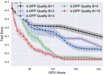
Finally, we study the performance with different choices of batch size $B$ in Fig. 14 which naturally confirms that the performance increases with larger batch size $B$.

Figure 14: Performance with different batch sizes $B$ on Imagenet. The result shows that the performance increases with larger batch size $B$, given the same wall-clock time budget (or batch iteration).

References

- Back (1996) Back, T. Evolutionary algorithms in theory and practice: evolution strategies, evolutionary programming, genetic algorithms. Oxford university press, 1996.
- Baker et al. (2017) Baker, B., Gupta, O., Naik, N., and Raskar, R. Designing neural network architectures using reinforcement learning. International Conference on Learning Representations, 2017.
- Berg et al. (1984) Berg, C., Christensen, J. P. R., and Ressel, P. Harmonic analysis on semigroups. Springer-Verlag, 1984.
- Bergstra et al. (2011) Bergstra, J. S., Bardenet, R., Bengio, Y., and Kégl, B. Algorithms for hyper-parameter optimization. In Advances in Neural Information Processing Systems, pp. 2546–2554, 2011.
- Burkard & Cela (1999) Burkard, R. E. and Cela, E. Linear assignment problems and extensions. In Handbook of combinatorial optimization, pp. 75–149. Springer, 1999.
- Contal et al. (2013) Contal, E., Buffoni, D., Robicquet, A., and Vayatis, N. Parallel gaussian process optimization with upper confidence bound and pure exploration. In Machine Learning and Knowledge Discovery in Databases, pp. 225–240. Springer, 2013.
- Desautels et al. (2014) Desautels, T., Krause, A., and Burdick, J. W. Parallelizing exploration-exploitation tradeoffs in gaussian process bandit optimization. The Journal of Machine Learning Research, 15(1):3873–3923, 2014.
- Do Ba et al. (2011) Do Ba, K., Nguyen, H. L., Nguyen, H. N., and Rubinfeld, R. Sublinear time algorithms for Earth Mover’s distance. Theory of Computing Systems, 48(2):428–442, 2011.
- Dong & Yang (2019) Dong, X. and Yang, Y. Searching for a robust neural architecture in four gpu hours. In Proceedings of the IEEE Conference on Computer Vision and Pattern Recognition, pp. 1761–1770, 2019.
- Dong & Yang (2020) Dong, X. and Yang, Y. Nas-bench-201: Extending the scope of reproducible neural architecture search. International Conference on Learning Representation, 2020.
- Elsken et al. (2019a) Elsken, T., Metzen, J. H., and Hutter, F. Efficient multi-objective neural architecture search via lamarckian evolution. International Conference on Learning Representation, 2019a.
- Elsken et al. (2019b) Elsken, T., Metzen, J. H., and Hutter, F. Neural architecture search: A survey. Journal of Machine Learning Research, 20(55):1–21, 2019b.
- Falkner et al. (2018) Falkner, S., Klein, A., and Hutter, F. Bohb: Robust and efficient hyperparameter optimization at scale. In International Conference on Machine Learning, pp. 1436–1445, 2018.
- Flamary & Courty (2017) Flamary, R. and Courty, N. Pot python optimal transport library. GitHub: https://github. com/rflamary/POT, 2017.
- Frazier (2018) Frazier, P. I. A tutorial on Bayesian optimization. arXiv preprint arXiv:1807.02811, 2018.
- Gao et al. (2010) Gao, X., Xiao, B., Tao, D., and Li, X. A survey of graph edit distance. Pattern Analysis and applications, 13(1):113–129, 2010.
- Garnett et al. (2010) Garnett, R., Osborne, M. A., and Roberts, S. J. Bayesian optimization for sensor set selection. In Proceedings of the 9th ACM/IEEE international conference on information processing in sensor networks, pp. 209–219, 2010.
- Ginsbourger et al. (2010) Ginsbourger, D., Le Riche, R., and Carraro, L. Kriging is well-suited to parallelize optimization. In Computational Intelligence in Expensive Optimization Problems, pp. 131–162. Springer, 2010.
- González et al. (2016) González, J., Dai, Z., Hennig, P., and Lawrence, N. D. Batch Bayesian optimization via local penalization. In International Conference on Artificial Intelligence and Statistics, pp. 648–657, 2016.
- Gopakumar et al. (2018) Gopakumar, S., Gupta, S., Rana, S., Nguyen, V., and Venkatesh, S. Algorithmic assurance: An active approach to algorithmic testing using Bayesian optimisation. In Advances in Neural Information Processing Systems, pp. 5465–5473, 2018.
- Hernández-Lobato et al. (2017) Hernández-Lobato, J. M., Requeima, J., Pyzer-Knapp, E. O., and Aspuru-Guzik, A. Parallel and distributed Thompson sampling for large-scale accelerated exploration of chemical space. In International Conference on Machine Learning, pp. 1470–1479, 2017.
- Jin et al. (2018) Jin, H., Song, Q., and Hu, X. Auto-keras: Efficient neural architecture search with network morphism. 2018.
- Kandasamy et al. (2018) Kandasamy, K., Neiswanger, W., Schneider, J., Poczos, B., and Xing, E. P. Neural architecture search with bayesian optimisation and optimal transport. In Advances in Neural Information Processing Systems, pp. 2016–2025, 2018.
- Kathuria et al. (2016) Kathuria, T., Deshpande, A., and Kohli, P. Batched Gaussian process bandit optimization via determinantal point processes. In Advances in Neural Information Processing Systems, pp. 4206–4214, 2016.
- Kondor & Lafferty (2002) Kondor, R. and Lafferty, J. Diffusion kernels on graphs and other discrete input spaces. In International Conference on Machine Learning, pp. 315–322, 2002.
- Kulesza & Taskar (2011) Kulesza, A. and Taskar, B. k-dpps: Fixed-size determinantal point processes. In Proceedings of the 28th International Conference on Machine Learning, pp. 1193–1200, 2011.
- Kulesza et al. (2012) Kulesza, A., Taskar, B., et al. Determinantal point processes for machine learning. Foundations and Trends® in Machine Learning, 5(2–3):123–286, 2012.
- Le & Nguyen (2021) Le, T. and Nguyen, T. Entropy partial transport with tree metrics: Theory and practice. In International Conference on Artificial Intelligence and Statistics, pp. 3835–3843, 2021.
- Le et al. (2019a) Le, T., Huynh, V., Ho, N., Phung, D., and Yamada, M. On scalable variant of wasserstein barycenter. arXiv preprint arXiv:1910.04483, 2019a.
- Le et al. (2019b) Le, T., Yamada, M., Fukumizu, K., and Cuturi, M. Tree-sliced variants of Wasserstein distances. In Advances in Neural Information Processing Systems, pp. 12283–12294, 2019b.
- Le et al. (2021) Le, T., Ho, N., and Yamada, M. Flow-based alignment approaches for probability measures in different spaces. In International Conference on Artificial Intelligence and Statistics, pp. 3934–3942, 2021.
- Li & Jamieson (2018) Li, L. and Jamieson, K. Hyperband: A novel bandit-based approach to hyperparameter optimization. Journal of Machine Learning Research, 18:1–52, 2018.
- Liu et al. (2018) Liu, H., Simonyan, K., Vinyals, O., Fernando, C., and Kavukcuoglu, K. Hierarchical representations for efficient architecture search. International Conference on Learning Representation, 2018.
- Liu et al. (2019) Liu, H., Simonyan, K., and Yang, Y. Darts: Differentiable architecture search. International Conference on Learning Representation, 2019.
- Luo et al. (2018) Luo, R., Tian, F., Qin, T., Chen, E., and Liu, T.-Y. Neural architecture optimization. In Advances in Neural Information Processing Systems, pp. 7816–7827, 2018.
- Mémoli (2011) Mémoli, F. Gromov–wasserstein distances and the metric approach to object matching. Foundations of computational mathematics, 11(4):417–487, 2011.
- Mémoli et al. (2019) Mémoli, F., Smith, Z., and Wan, Z. Gromov-hausdorff distances on -metric spaces and ultrametric spaces. arXiv preprint arXiv:1912.00564, 2019.
- Mémoli et al. (2021) Mémoli, F., Munk, A., Wan, Z., and Weitkamp, C. The ultrametric gromov-wasserstein distance. arXiv preprint arXiv:2101.05756, 2021.
- Messmer & Bunke (1998) Messmer, B. T. and Bunke, H. A new algorithm for error-tolerant subgraph isomorphism detection. IEEE transactions on pattern analysis and machine intelligence, 20(5):493–504, 1998.
- Nguyen & Osborne (2020) Nguyen, V. and Osborne, M. A. Knowing the what but not the where in Bayesian optimization. In International Conference on Machine Learning, pp. 7317–7326. PMLR, 2020.
- Nguyen et al. (2016) Nguyen, V., Rana, S., Gupta, S. K., Li, C., and Venkatesh, S. Budgeted batch Bayesian optimization. In 16th International Conference on Data Mining (ICDM), pp. 1107–1112, 2016.
- Nguyen et al. (2020) Nguyen, V., Schulze, S., and Osborne, M. A. Bayesian optimization for iterative learning. In Advances in Neural Information Processing Systems, 2020.
- Parker-Holder et al. (2020) Parker-Holder, J., Nguyen, V., and Roberts, S. J. Provably efficient online hyperparameter optimization with population-based bandits. Advances in Neural Information Processing Systems, 33, 2020.
- Peyré & Cuturi (2019) Peyré, G. and Cuturi, M. Computational optimal transport. Foundations and Trends in Machine Learning, 11(5-6):355–607, 2019.
- Pham et al. (2018) Pham, H., Guan, M., Zoph, B., Le, Q., and Dean, J. Efficient neural architecture search via parameters sharing. In International Conference on Machine Learning, pp. 4095–4104, 2018.
- Rahimi & Recht (2007) Rahimi, A. and Recht, B. Random features for large-scale kernel machines. In Advances in Neural Information Processing Systems, pp. 1177–1184, 2007.
- Rana et al. (2017) Rana, S., Li, C., Gupta, S., Nguyen, V., and Venkatesh, S. High dimensional Bayesian optimization with elastic Gaussian process. In Proceedings of the 34th International Conference on Machine Learning, pp. 2883–2891, 2017.
- Rasmussen (2006) Rasmussen, C. E. Gaussian processes for machine learning. 2006.
- Real et al. (2017) Real, E., Moore, S., Selle, A., Saxena, S., Suematsu, Y. L., Tan, J., Le, Q. V., and Kurakin, A. Large-scale evolution of image classifiers. In Proceedings of the 34th International Conference on Machine Learning, pp. 2902–2911, 2017.
- Real et al. (2019) Real, E., Aggarwal, A., Huang, Y., and Le, Q. V. Regularized evolution for image classifier architecture search. In Proceedings of the AAAI conference on Artificial Intelligence, volume 33, pp. 4780–4789, 2019.
- Ru et al. (2020) Ru, B., Alvi, A. S., Nguyen, V., Osborne, M. A., and Roberts, S. J. Bayesian optimisation over multiple continuous and categorical inputs. In International Conference on Machine Learning, 2020.
- Ru et al. (2021) Ru, B., Wan, X., Dong, X., and Osborne, M. A. Interpretable neural architecture search via bayesian optimisation with weisfeiler-lehman kernels. International Conference on Learning Representation, 2021.
- Sciuto et al. (2019) Sciuto, C., Yu, K., Jaggi, M., Musat, C., and Salzmann, M. Evaluating the search phase of neural architecture search. arXiv preprint arXiv:1902.08142, 2019.
- Semple & Steel (2003) Semple, C. and Steel, M. Phylogenetics. Oxford Lecture Series in Mathematics and its Applications, 2003.
- Shah et al. (2018) Shah, S. A. R., Wu, W., Lu, Q., Zhang, L., Sasidharan, S., DeMar, P., Guok, C., Macauley, J., Pouyoul, E., Kim, J., et al. Amoebanet: An sdn-enabled network service for big data science. Journal of Network and Computer Applications, 119:70–82, 2018.
- Shahriari et al. (2016) Shahriari, B., Swersky, K., Wang, Z., Adams, R. P., and de Freitas, N. Taking the human out of the loop: A review of Bayesian optimization. Proceedings of the IEEE, 104(1):148–175, 2016.
- Smola & Kondor (2003) Smola, A. J. and Kondor, R. Kernels and regularization on graphs. In Learning theory and kernel machines, pp. 144–158. Springer, 2003.
- Snoek et al. (2012) Snoek, J., Larochelle, H., and Adams, R. P. Practical Bayesian optimization of machine learning algorithms. In Advances in Neural Information Processing Systems, pp. 2951–2959, 2012.
- Snoek et al. (2015) Snoek, J., Rippel, O., Swersky, K., Kiros, R., Satish, N., Sundaram, N., Patwary, M., Prabhat, M., and Adams, R. Scalable Bayesian optimization using deep neural networks. In Proceedings of the 32nd International Conference on Machine Learning, pp. 2171–2180, 2015.
- Springenberg et al. (2016) Springenberg, J. T., Klein, A., Falkner, S., and Hutter, F. Bayesian optimization with robust bayesian neural networks. In Advances in Neural Information Processing Systems, pp. 4134–4142, 2016.
- Srinivas et al. (2010) Srinivas, N., Krause, A., Kakade, S., and Seeger, M. Gaussian process optimization in the bandit setting: No regret and experimental design. In Proceedings of the 27th International Conference on Machine Learning, pp. 1015–1022, 2010.
- Suganuma et al. (2017) Suganuma, M., Shirakawa, S., and Nagao, T. A genetic programming approach to designing convolutional neural network architectures. In Proceedings of the Genetic and Evolutionary Computation Conference, pp. 497–504, 2017.
- Villani (2003) Villani, C. Topics in optimal transportation. American Mathematical Soc., 2003.
- Vishwanathan et al. (2010) Vishwanathan, S. V. N., Schraudolph, N. N., Kondor, R., and Borgwardt, K. M. Graph kernels. Journal of Machine Learning Research, 11(Apr):1201–1242, 2010.
- Wallis et al. (2001) Wallis, W. D., Shoubridge, P., Kraetz, M., and Ray, D. Graph distances using graph union. Pattern Recognition Letters, 22(6-7):701–704, 2001.
- Wan et al. (2021) Wan, X., Nguyen, V., Ha, H., Ru, B., Lu, C., and Osborne, M. A. Think global and act local: Bayesian optimisation over high-dimensional categorical and mixed search spaces. In International Conference on Machine Learning, 2021.
- Wang et al. (2020) Wang, L., Zhao, Y., Jinnai, Y., Tian, Y., and Fonseca, R. Alphax: exploring neural architectures with deep neural networks and monte carlo tree search. The Thirty-Fourth AAAI Conference on Artificial Intelligence, 2020.
- Wang et al. (2018) Wang, Z., Gehring, C., Kohli, P., and Jegelka, S. Batched large-scale Bayesian optimization in high-dimensional spaces. In International Conference on Artificial Intelligence and Statistics, pp. 745–754, 2018.
- White et al. (2021) White, C., Neiswanger, W., and Savani, Y. Bananas: Bayesian optimization with neural architectures for neural architecture search. In Proceedings of the AAAI Conference on Artificial Intelligence, 2021.
- Xie & Yuille (2017) Xie, L. and Yuille, A. Genetic cnn. In Proceedings of the IEEE International Conference on Computer Vision, pp. 1379–1388, 2017.
- Xie et al. (2019) Xie, S., Zheng, H., Liu, C., and Lin, L. Snas: stochastic neural architecture search. International Conference on Learning Representation, 2019.
- Yao et al. (2020) Yao, Q., Xu, J., Tu, W.-W., and Zhu, Z. Efficient neural architecture search via proximal iterations. In AAAI Conference on Artificial Intelligence, 2020.
- Ying et al. (2019) Ying, C., Klein, A., Christiansen, E., Real, E., Murphy, K., and Hutter, F. Nas-bench-101: Towards reproducible neural architecture search. In International Conference on Machine Learning, pp. 7105–7114, 2019.
- Zhong et al. (2018) Zhong, Z., Yan, J., Wu, W., Shao, J., and Liu, C.-L. Practical block-wise neural network architecture generation. In Proceedings of the IEEE conference on Computer Vision and Pattern Recognition, pp. 2423–2432, 2018.
- Zoph & Le (2017) Zoph, B. and Le, Q. V. Neural architecture search with reinforcement learning. International Conference on Representation Learning, 2017.