Active Sampling for Min-Max Fairness
Abstract
We propose simple active sampling and reweighting strategies for optimizing min-max fairness that can be applied to any classification or regression model learned via loss minimization. The key intuition behind our approach is to use at each timestep a datapoint from the group that is worst off under the current model for updating the model. The ease of implementation and the generality of our robust formulation make it an attractive option for improving model performance on disadvantaged groups. For convex learning problems, such as linear or logistic regression, we provide a fine-grained analysis, proving the rate of convergence to a min-max fair solution.
1 Introduction
A model trained on a dataset containing multiple demographic groups typically has unequal error rates across the different groups, either because some groups are underrepresented in the training data or the underlying learning task is inherently harder for particular groups. Many existing fairness notions aim to equalize the performance on different demographic groups (e.g., Hardt et al., 2016; Zafar et al., 2019), which can result in deliberately down-grading the performance on the better off groups and unnecessarily reducing overall performance. This degradation of performance can correspond to a loss of access to relevant services, which is referred to as “leveling-down” in law and ethics where it has received substantial criticism (Holtug, 1998; Temkin, 2000; Doran, 2001; Mason, 2001; Brown, 2003; Christiano and Braynen, 2008). In contrast, min-max notions of fairness offer an alternative approach. These notions “level-up”, by adopting an optimization perspective that prioritizes improving the model’s performance on the group for which performance is the worst. Such optimizations only degrade the performance on a group if it will improve the performance on the worst off group (Martinez et al., 2020; Diana et al., 2021).
In this paper, we propose simple and theoretically principled algorithms for min-max fairness (formally defined in Section 2). We provide a general template in Algorithm 1. The key idea underlying our approach is to adaptively sample or reweight data from worst off groups. The intent is that by providing additional data for these groups, or increasing the weights associated with them, we improve the model’s performance on these groups. This is a compellingly simple approach to mitigating loss disparity between groups, and we show that for convex learning problems such methods indeed provably minimize the maximum per-group loss.
We consider two concrete variants of Algorithm 1. The first one (Algorithm 2) simply samples a point from the worst off group and updates model parameters via stochastic gradient descent. We show in Theorem 1 that Algorithm 2 converges to a min-max fair solution at a rate of (as a function of the number of iterations ), assuming a convex loss function. Our second approach (Algorithm 3), accelerated min-max gradient descent, converges to a min-max fair solution at a faster rate of .
The accelerated Algorithm 3 is based on an adaptive reweighting scheme and performs in each iteration a gradient descent step for optimizing a weighted population loss. In contrast, Algorithm 2 samples, in each iteration, a datapoint from the worst off group and uses it for performing a stochastic gradient descent step. While Algorithm 3 achieves a faster rate of convergence, Algorithm 2 is conceptually simpler, easier to implement and efficient in practice due to the stochastic nature of the updates. We also provide finite sample generalization bounds for Algorithm 2. We present an empirical evaluation of both our proposed algorithms in Section 5.
2 Preliminaries
Let be our data space; any represents a population sample containing both the observed features and the unobserved label. We assume that there are disjoint demographic groups, indexed by the set .111 Sometimes we want to be fair w.r.t. demographic groups that are not disjoint, e.g., to men and women and also to old and young people. In this case, as it is standard in the literature, we simply consider all intersections of these groups, i.e., young females, young males, etc..
Let be a family of distributions over , where is the distribution of the data for group . Let denote a vector of mixture weights over groups. Given any , we define the mixture distribution on as follows: we first sample a group index , and then we sample from the randomly chosen group .
The models considered are based on a parameterized family of functions , where each operates on examples and is a -dimensional parameter space. We assume that is a compact convex set. We evaluate each according to a loss function , and we assume the loss to be convex in for any fixed :
Assumption 1.
For any , the function is convex in .
Assumption 1 is satisfied in several common scenarios, e.g., when is linear in and is the standard logistic loss or hinge loss (binary classification), the cross entropy loss composed with softmax activation (multiclass classification), or the squared loss (regression). While we use throughout the paper to refer to the gradient, we do not strictly need to be differentiable as we may consider any sub-gradient instead.
Given a distribution and any , we define the expected loss of with respect to as
Similarly, given mixture weights , we consider the performance of with respect to . Thus
For each group we assume we have an IID sample of examples . We use to represent the empirical distribution over these samples. Hence,
Throughout, we use the notation to refer to the -projection of point onto compact convex set , that is .
Our goal is to learn a model that is min-max fair w.r.t. the demographic groups. This means that satisfies
Remark 1.
A criticism of the min-max approach to fairness is that it puts too much focus on improving the performance of a single group. If some class is particularly hard to learn, so that any will have a large value , larger than for all other classes , then the training procedure will aim to optimize the loss with respect to only . This is a reasonable concern, but we can mitigate it by considering blended distributions: let be a trade-off parameter, and define the mixture distribution
where is the true population-level distribution; that is, the full population is made up of a mixture of subpopulations weighted by the true mixture . If we run our min-max fairness procedures on the blended distributions instead of on , we are biasing our algorithm, with bias parameter , to focus more on the full population and less on any particular group.
3 Algorithms and Analysis
Here we present formal versions of Algorithm 1, and analyze their theoretical performance. To formalize Algorithm 1 fully, we describe how we evaluate which group has the highest loss in each iteration, and how we either sample additional data from that group or reweight and update the model. Both algorithms use their updating schemes to reduce their training error on the min-max objective, and while we also present theorems which bound the test error as well, this work does not use reweighting or resampling to explicitly decrease generalization error.
3.1 Stochastic Optimization
Algorithm 2 maintains a validation set, that is a fixed comparison sample set on which the group-specific loss is repeatedly measured. It samples a fresh point from the group with highest loss on the comparison set, then takes a single gradient step in the direction of that fresh sample. Its performance is governed by two quantities: the regret term, which decreases with the number of iterations , and the uniform deviation bound of the comparisons of group-specific loss.
As is common in gradient descent, the following proof assumes that the Lipschitz constant and a domain radius are known. When this is not the case, the step size is typically tuned empirically.
Theorem 1.
Assume we have a function which guarantees that
with probability at least . Let and . With , Algorithm 2 ensures that
with probability at least .
Proof.
This bound is obtained by combining a number of classical results from empirical process theory, as well as common tricks from using online convex optimization tools to solve min-max problems. This sequence of steps is given in Figure 1, with further discussion here.
One observes that we need to swap between and on two separate inequalities, and on each we have to add the deviation bound ; the factor is necessary because we need a union bound over all rounds. We then replace with , which is valid since is independent of , is distributed according to , and we have the outer expectation over all (more details on this technique can be found in the paper of Cesa-Bianchi et al., 2004). Next, since the ’s are chosen using the Online Gradient Descent (OGD) algorithm on loss functions , we can immediately apply the OGD regret bound—see Hazan (2019) for details.
The most subtle part of this proof may be the final two observations. The sequence is generated stochastically and sequentially, where each may depend on the previous samples chosen. But in the end, the sample is produced by taking some combination of samples from the various , and ultimately we marginalize the quantity over the randomness generated by . On average, the ’s in will have been drawn from some mixture over the various groups, and we refer to those mixture weights as . It then follows by this observation that . Finally, since , we upper bound with to complete the proof. ∎
While not the focus of our paper, it is easy enough to give a uniform deviation bound as Theorem 1 employs.
Lemma 1.
With probability at least , for every and for every it holds that
where is some constant and P-dim is the pseudo-dimension of the class (Pollard, 1990).
Proof.
This follows from a standard uniform convergence argument over for any fixed group , as is a sample of IID points drawn from . Taking a union bound over all groups yields the bound. ∎
This implies that the total error of using Algorithm 2 is comprised of two terms, one upper bounding the optimization error (which decays with ), and the generalization error, which is governed by the sample size of the smallest dataset across all groups.
A key benefit of Theorem 1 is that it provides both an optimization guarantee as well as a sample complexity bound. The proof’s core is the classical “online to batch conversion” (Cesa-Bianchi et al., 2004) that provides generalization based on regret bounds, combined with tools from min-max optimization.
One downside of this method is that it relies on having two sources of data: a “comparison set” for each , as well as the ability to draw fresh (independent) samples from each . Alternatively, we consider a version that only focuses on training error that reweights rather than samples fresh data, by considering drawn from . This variant will still allow for the min-max empirical risk to decay at the standard rate.
Corollary 1.
Remark 2 (Mini-batching).
Many online training scenarios use mini-batch gradient updates, where instead of a single sample a set of samples is taken, an average gradient is computed across these samples, and the average gradient is used to update the current parameter estimate. Indeed, it requires a straightforward modification to implement mini-batch training in Algorithm 2. While this may have practical benefits, providing faster empirical training times, we note that this is not likely to provide improved theoretical guarantees. Our convergence guarantee in Theorem 1 still applies in the mini-batch setting, with convergence depending on the number of updates , rather than the total amount of data used. Batches of size then require times more data overall for the same convergence guarantee. One might hope for a decrease in variance from the mini-batch averaging, and indeed this often empirically leads to better convergence, though not promised by our results.
3.2 Accelerated Optimization
Algorithm 3’s optimization error shrinks much faster as a function of . However, it is non-stochastic and has a more complex update rule. This algorithm explicitly maintains a distribution over groups which it updates relative to the current group losses, increasing the probability mass assigned to groups with higher loss. Then the algorithm takes a gradient step with respect to the full, weighted distribution over (empirical) group distributions. While each iteration requires a full pass over the data, the convergence rate is rather than .
Unlike Algorithm 2, Algorithm 3 does not have a natural “sampling” analogue. The update rule is with respect to the entire weighted empirical distribution, rather than a single datapoint. Below we present the main algorithmic guarantee associated with the algorithm. See Appendix A for the proof.
Theorem 2.
Remark 3 (Averaging versus final iterate).
A careful reader may note that Algorithms 2 and 3 output a time-weighted average , whereas in typical online training methods one simply outputs the final iterate . Indeed, for the min-max framework we propose, our theory requires returning the average iterate. Some work exists on last-iterate convergence for special cases of min-max optimization (Abernethy et al., 2021), but this is beyond the scope of the present work.
4 Related Work
| US | UK | Other | Overall | ||
| Diana et al. (2021) | 0.4035 | 0.5894 | 0.4710 | 0.5166 | Log loss |
| Martinez et al. (2020) | 0.4122 | 0.5889 | 0.4771 | 0.5198 | |
| OURS (Alg. 2 with TRAIN=VAL; Avg. over 5 runs) | 0.4114 | 0.5889 | 0.4766 | 0.5195 | |
| OURS (Alg. 2 with SMALL VAL; Avg. over 5 runs) | 0.4112 | 0.5889 | 0.4766 | 0.5195 | |
| OURS (Algorithm 3) | 0.4108 | 0.5889 | 0.4761 | 0.5193 | |
| Diana et al. (2021) | 0.1566 | 0.2964 | 0.2173 | 0.2432 | 01 loss |
| Martinez et al. (2020) | 0.1598 | 0.2950 | 0.2183 | 0.2435 | |
| OURS (Alg. 2 with TRAIN=VAL; Avg. over 5 runs) | 0.1634 | 0.2971 | 0.2218 | 0.2463 | |
| OURS (Alg. 2 with SMALL VAL; Avg. over 5 runs) | 0.1601 | 0.2960 | 0.2211 | 0.2446 | |
| OURS (Algorithm 3) | 0.1598 | 0.2960 | 0.2183 | 0.2440 |
Fair ML.
There is a large body of work on fairness in machine learning (Barocas et al., 2018), much of it focusing on supervised learning. Many fairness notions balance performance measures across different groups (e.g., Hardt et al., 2016). These notions suffer from the “leveling-down” discussed in the introduction. Min-max fairness notions have been proposed as a remedy.
Min-max fairness.
Martinez et al. (2020) consider the search for min-max Pareto optimal classifiers and present structural results regarding the case of unbounded hypothesis sets. By appropriately reparameterizing the space, they show that one can, in principle, model the case of learning min-max Pareto optimal classifiers over the class of deep neural networks. Martinez et al. propose an algorithm to find optimal classifiers (based on sub-gradient descent), but unlike our work, their proposed algorithm has no performance guarantees, and is not guaranteed to converge.
Diana et al. (2021) propose a multiplicative weights update based method to achieve min-max fairness. While they do not require convexity, they assume access to a weighted empirical risk minimization (ERM) oracle, and it is unclear how to implement such oracles in a non-convex setting. Furthermore, the analysis in Diana et al. (2021) is only carried out in the population setting where it is assumed that certain weighted ERM problems can be exactly optimized over the distribution. As a result, their work ignores the complexity of the analysis arising from the stochastic nature of gradient updates. One key contribution of our work is the analysis of gradient-based updates, which allow for more efficient computation and the use of highly-optimised frameworks and tools. Finally, at least in the non-convex case, the hypothesis output by Diana et al. (2021) needs to be randomized, which can be problematic in scenarios strongly affecting people (Cotter et al., 2019b).
A previous arxiv version of this paper introduced a restricted variant of Algorithm 1, where a single sample was drawn from the worst off group, and each round’s model was the global optimum on the current dataset, and analyzed its behaviour. Shekhar et al. (2021) claimed that the sampling scheme proposed in our previous draft and closely related to our Algorithm 1 converges to min-max fair solutions. While their paper does not impose convexity constraints, their algorithm has no rate of convergence guarantees, and their assumptions (particularly Assumption 2) needed to prove convergence frequently fail to hold in practice.222 Their Assumption 2 states “For any two distinct attributes , we must have , for any .” This rarely holds in practice. In particular, let be a min-max optimal predictor. Consider a group with largest loss under : we know that for any other group . When this inequality is strict and , we actually know that , or mixing and would reduce the min-max risk of . So, in many applications of interest (for instance, where the min-max optimal predictor has a unique worst off group), their assumption will not hold—it never held in any of our experiments. We improve those results empirically and theoretically and guarantee fast rates of convergence.
Min-max optimization.
Many problems beyond fairness can be formulated as min-max optimization problems, and the study of generic methods for solving these remains an active field of research (e.g., Thekumparampil et al., 2019; Razaviyayn et al., 2020; Ouyang and Xu, 2021). We are unaware of any generic methods that would be appropriate for our fairness problem with a discrete group variable.
Group reweighting.
Other works study the problem of debiasing a dataset via group reweighting. Li and Vasconcelos (2019) propose a reweighting scheme to reduce representation bias. While based on a min-max formulation, their problem setting is different to ours. Rolf et al. (2021) study structural properties of optimal group allocations for a dataset. They present structural results regarding the nature of optimal allocations, but no algorithmic results.
Agarwal et al. (2019) consider a fair regression problem under a bounded group loss constraint, which in their setting is equivalent to finding a min-max fair classifier. Similar to Diana et al. (2021), they design a near optimal regressor assuming access to a weighted risk minimization oracle that can be optimized exactly on the population. Achieving fairness under bounded loss constraints assuming oracle access has also been studied by Cotter et al. (2019a).
Active sampling.
Active / adaptive sampling lies at the heart of active learning (Settles, 2010). Related to our work is the paper by Anahideh and Asudeh (2020). In each round their sampling strategy queries the label of a datapoint that is both informative and expected to yield a classifier with small violation of a fairness measure (they do not consider min-max fairness but mainly demographic parity, which requires the classifier’s prediction to be independent of group membership). Unlike our work, their approach requires training a classifier for every datapoint which might be queried before actually querying a datapoint, resulting in a significant computational overhead. Moreover, their work does not provide any theoretical analysis. Also related is the paper by Noriega-Campero et al. (2019), who propose to actively collect additional features for datapoints to equalize the performance on different groups.
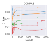
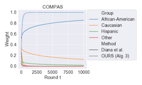
| African-American | Caucasian | Hispanic | Other | Overall | ||
| Diana et al. (2021) | 0.6200 | 0.6132 | 0.6104 | 0.5804 | 0.6145 | Log loss |
| Martinez et al. (2020) | 0.6196 | 0.6162 | 0.6129 | 0.5830 | 0.6158 | |
| OURS (Algorithm 3) | 0.6196 | 0.6161 | 0.6127 | 0.5828 | 0.6156 | |
| Diana et al. (2021) | 0.3279 | 0.3292 | 0.3150 | 0.3074 | 0.3260 | 01 loss |
| Martinez et al. (2020) | 0.3309 | 0.3370 | 0.3234 | 0.3185 | 0.3316 | |
| OURS (Algorithm 3) | 0.3309 | 0.3370 | 0.3234 | 0.3185 | 0.3316 |
5 Experiments
Before presenting empirical results,333Code available on https://github.com/amazon-research/active-sampling-for-minmax-fairness we once more highlight the key advantages of our method over existing ones: (a) simplicity and computational efficiency—we only perform one (stochastic) gradient step in every iteration, while the other methods fully retrain in every iteration; (b) stronger convergence guarantees—our proposed Algorithm 2 (Algorithm 3) is guaranteed to converge at a rate of () SGD (GD) steps. In contrast, the algorithm presented in Diana et al. (2021) is guaranteed to converge at a rate of oracle calls, and Martinez et al. (2020) do not prove convergence of their proposed algorithm.
Our online stochastic approach is substantially faster than the fully deterministic approaches that exactly solve subproblems at each iteration. To avoid being mislead by implementation details, such as the choice of implementation language, we consider a proxy for runtime: namely, the number of times any datapoint is examined. Under this metric, the cost of computing a single SGD update of mini-batch size is ; the cost of evaluating the objective w.r.t. a single point is ; while the cost of evaluating the objective for every datapoint of a dataset of size is . Logistic regression has a cost of where is the number of iterations needed to reach convergence.
Looking at Algorithm 2, we see that a significant bottleneck per iteration is line 3, which evaluates the loss over a validation set. Set size is potentially important: too small and the method may not reliably select the worst off group, but if it is too large, it will needlessly hurt runtime. As such, we evaluate using small validation sets containing random members of each group, and larger validation sets. For all experiments we use a mini-batch size of 32.
We compare with the public code of both Diana et al. (2021) and Martinez et al. (2020). When evaluating efficiency, we focus on the method of Diana et al. (2021), however, since the method of Martinez et al. (2020) does not come with theoretical guarantees of convergence (and as such it is incomparable to our methods anyway) and their experimental evaluation does not look at the evolution of iterates over time but only at the final iterate. As for our proposed strategy, we focus on Algorithm 2 as the efficient variant of our general strategy (Algorithm 1) in the convex case; however, we also study the performance of Algorithm 3, and we run Algorithm 2 without averaging using a simple neural network as classification model to study the non-convex case.
Similarly to Diana et al., we report both optimization and generalization performance. To evaluate optimization performance, we use small datasets and report results on the training data. When studying generalization performance, we consider a large dataset and report results on a held-out test set. Since our strategy (Algorithms 1 or 2) is randomized, we show its results for five runs with different random seeds. See Appendix B.1 for implementation details.
Heuristics for estimating and . Algorithm 3 requires estimates of the values , and in order to set the parameters and . We use the same method of estimating them for both experiments shown in Figure 3 and the table of Figure 2, respectively: as the data is whitened, we simply take , where is the number of parameters in our logistic regression model, as an upper bound for the gradient of logistic regression. For , we run unweighted logistic regression over the entire dataset and use this as the initialisation of our model. Finally, we take as an approximate estimate of the size of the domain.
| [0-50) | [50-60) | [60-70) | [70-80) | [80-90) | [0-50) | [50-60) | [60-70) | [70-80) | [80-90) | ||||
| Diana et al. (2021) | Train | 0.6327 | 0.6425 | 0.6474 | 0.6550 | 0.6473 | Log loss | 0.3256 | 0.3418 | 0.3500 | 0.3626 | 0.3498 | |
| Test | 0.6357 | 0.6443 | 0.6495 | 0.6563 | 0.6509 | 0.3304 | 0.3450 | 0.3537 | 0.3652 | 0.3556 | 01 loss | ||
| Martinez et al. (2020) | Train | 0.6145 | 0.6219 | 0.6289 | 0.6458 | 0.6439 | 0.3228 | 0.3326 | 0.3435 | 0.3616 | 0.3573 | ||
| Test | 0.6113 | 0.6263 | 0.6329 | 0.6448 | 0.6456 | 0.3198 | 0.3396 | 0.3513 | 0.3650 | 0.3611 | |||
| OURS (Alg. 2; Avg. 5 runs) | Train | 0.6161 | 0.6232 | 0.6299 | 0.6458 | 0.6439 | 0.3240 | 0.3333 | 0.3442 | 0.3618 | 0.3579 | ||
| Test | 0.6129 | 0.6277 | 0.6337 | 0.6449 | 0.6455 | 0.3197 | 0.3401 | 0.3511 | 0.3650 | 0.3600 |
Performance on smaller datasets. We compare Algorithms 2 and 3 with Diana et al. (2021) and Martinez et al. (2020) on the Drug Consumption dataset (Fehrman et al., 2015) and the COMPAS dataset (Angwin et al., 2016), respectively. We provide some details about the datasets used in our experiments in Appendix B.2.
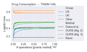
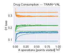
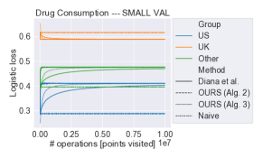
On the Drug Consumption dataset, we train a logistic regressor to predict if an individual consumed cannabis within the last decade or not. The groups that we want to be fair to are defined by an individual’s country. The dataset contains 1885 records. We use the entire dataset for training (sampling and performing SGD updates) and for reporting performance metrics. We either use the entire dataset or a small subset comprising 20 datapoints sampled uniformly at random from each group as validation set (for determining the group with the highest loss).
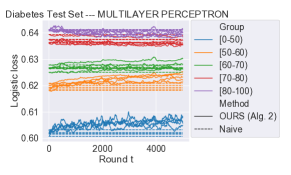
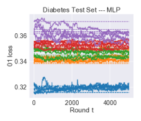
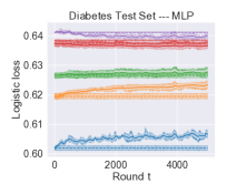
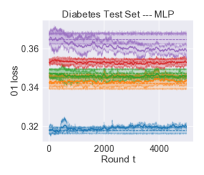
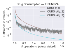
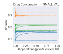
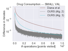
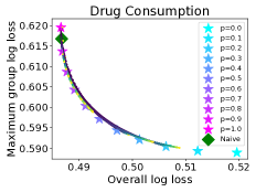
Figure 2 shows the results. The plots show the loss and error for each group over the run of our algorithms or that of Diana et al. (2021). Alongside loss or error curves, we also plot baseline curves that are obtained by training a classifier or regressor using standard SGD on the training data (dashed lines; denoted by Naive). The figure also provides a plot showing trade-off curves, trading off the maximum group loss vs the overall population loss. For Diana et al. the curve is obtained by varying the parameter in a variant of their algorithm, for our strategy we exploit the simple modification discussed in Remark 1: before determining the worst off group, we flip a biased coin and with probability sample a datapoint from the whole population and with probability sample from the worst off group. By varying the parameter , we generate the trade-off curve. The table shows the performance metrics for the model obtained in the final iteration of an algorithm (including the algorithm of Martinez et al. (2020)).
The loss (and also the error) of the worst off group decreases over time, while increasing for other groups. This is consistent with Section 3, which guarantees improved performance on the highest-loss group, but not for the other groups. In terms of the solution found in the final iteration, we perform similarly to Diana et al. (2021) and Martinez et al. (2020) with all methods accurately solving the same objective and finding similar cost solutions (cf. the table in Figure 2). Also the two trade-off curves are almost identical.
Very clear trends can be seen in the graphs. While around operations are required for Diana et al. (2021) to converge (this is particular apparent in the blue curve representing loss on the US), our approaches converge much faster. In particular, the intrinsic volatility of the SGD update is largely masked by the fast convergence of our approach with all runs converging much faster than any other approach, leading to multiple overlayed plots. The performance benefit is even more extreme when a small validation set is used. Here convergence looks near instantaneous when plotted on a scale that allows us to also see the behavior of the algorithm by Diana et al.. In general, despite its better performance guarantees, our deterministic accelerated version has comparable performance to Algorithm 2 with a large validation set, and lies midway in performance between Algorithm 2 with a small validation set and Diana et al. (2021). Note that as the parameters and are estimated heuristically, it is likely that better performance could be obtained if they were known; however, we felt it was more informative to report the performance obtained without tuning.
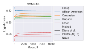
In Figure 3, we evaluate Algorithm 3 on the COMPAS dataset (Angwin et al., 2016) and train a logistic regression classifier to predict recidivism. The graphs show a comparison with Diana et al. (2021). For our method a single iteration corresponds to one step of gradient descent, while Diana et al. require the computation of an optimal classifier in each iteration. Despite this, we still converge substantially faster per iteration.
Generalization on a larger dataset. In Table 1, we evaluate on the Diabetes 130-US Hospitals dataset (Strack et al., 2014). The goal is to predict whether a patient was readmitted to hospital, and we want to be fair with respect to different age groups. We train a linear logistic classifier. The Diabetes dataset contains 101766 records, which we split into a training, validation, and a held-out test set of equal size. The latter is not used in training. We initialize our classifier training on a subset of 2000 training points.
All methods achieve similar loss and error, both when comparing between training and test sets and when comparing the various methods. The former illustrates the good generalization performance of the algorithms. The results for our Algorithm 2 and the method by Martinez et al. (2020) are even more similar to each other than compared to the method by Diana et al. (2021).
Algorithm 2 in non-convex learning. Minus the averaging step, Algorithm 2 can also be applied, without guarantees, to non-convex learning problems including neural network training. We demonstrate this by training a simple multilayer perceptron (MLP) with Algorithm 2 on the Diabetes dataset, as in the setting of Table 1. Results are shown in Figure 4. The plots show the per-group logistic losses and classification errors on the test set. We improve the loss and the error of the worst off group compared to the naive baseline.
6 Discussion
Potential harms. Implicit to min-max fairness is the idea that the labels are accurate and a trained classifier should reproduce them with high fidelity. As argued by Wachter et al. (2021), where this is not the case, for example: where racially-biased law enforcement practices make stop and arrest rates a poor surrogate for criminal activity (Baumgartner et al., 2018); where hiring data is based on biased historic practices (Harvie et al., 1998); or when using existing diagnoses to train skin cancer detection (Gupta et al., 2016); min-max fairness along with other error-based fairness notions can give rise to classifiers that mimic the biases present in the data, which if used to make substantive decisions about individuals can perpetuate inequality.
Our contribution. We present a novel approach to min-max algorithmic fairness. In contrast to existing approaches, our approach stands out both for its efficient stochastic nature and easy-to-implement formulations and its guaranteed convergence rates. Our experiments on real-world datasets show the merits of our approach.
Acknowledgements
Jamie Morgenstern and Jie Zhang acknowledge funding from the NSF AI Institute for the Foundations of Machine Learning (IFML), an NSF Career award, and the Simons Collaborative grant on Theory of Algorithmic Fairness.
References
- Abernethy et al. (2021) J. Abernethy, K. Lai, and A. Wibisono. Last-iterate convergence rates for min-max optimization: Convergence of hamiltonian gradient descent and consensus optimization. In International Conference on Algorithmic Learning Theory (ALT), 2021.
- Agarwal et al. (2019) A. Agarwal, M. Dudík, J. Langford, and Z. S. Wu. Fair regression: Quantitative definitions and reduction-based algorithms. In International Conference on Machine Learning (ICML), 2019.
- Anahideh and Asudeh (2020) H. Anahideh and A. Asudeh. Fair active learning. arXiv:2001.01796 [cs.LG], 2020.
- Angwin et al. (2016) J. Angwin, J. Larson, S. Mattu, and L. Kirchner. Propublica—machine bias, 2016. https://www.propublica.org/article/machine-bias-risk-assessments-in-criminal-sentencing.
- Barocas et al. (2018) S. Barocas, M. Hardt, and A. Narayanan. Fairness and Machine Learning. fairmlbook.org, 2018. http://www.fairmlbook.org.
- Baumgartner et al. (2018) F. R. Baumgartner, D. A. Epp, and K. Shoub. Suspect citizens: What 20 million traffic stops tell us about policing and race. Cambridge University Press, 2018.
- Brown (2003) C. Brown. Giving up levelling down. Economics and Philosophy, 19(1):111, 2003.
- Cesa-Bianchi et al. (2004) N. Cesa-Bianchi, A. Conconi, and C. Gentile. On the generalization ability of on-line learning algorithms. IEEE Transactions on Information Theory, 50(9):2050–2057, 2004.
- Chiang et al. (2012) C.-K. Chiang, T. Yang, C.-J. Lee, M. Mahdavi, C.-J. Lu, R. Jin, and S. Zhu. Online optimization with gradual variations. In Conference on Learning Theory (COLT), 2012.
- Christiano and Braynen (2008) T. Christiano and W. Braynen. Inequality, injustice and levelling down. Ratio, 21(4):392–420, 2008.
- Cotter et al. (2019a) A. Cotter, H. Jiang, and K. Sridharan. Two-player games for efficient non-convex constrained optimization. In International Conference on Algorithmic Learning Theory (ALT), 2019a.
- Cotter et al. (2019b) A. Cotter, H. Narasimhan, and M. Gupta. On making stochastic classifiers deterministic. In Neural Information Processing Systems (NeurIPS), 2019b.
- Diana et al. (2021) E. Diana, W. Gill, M. Kearns, K. Kenthapadi, and A. Roth. Minimax group fairness: Algorithms and experiments. In AAAI/ACM Conference on AI, Ethics, and Society (AIES), 2021. Code available on https://github.com/amazon-research/minimax-fair.
- Doran (2001) B. Doran. Reconsidering the levelling-down objection against egalitarianism. Utilitas, 13(1):65–85, 2001.
- Dua and Graff (2019) D. Dua and C. Graff. UCI Machine Learning Repository. University of California, Irvine, School of Information and Computer Sciences, 2019. http://archive.ics.uci.edu/ml.
- Fehrman et al. (2015) E. Fehrman, A. K. Muhammad, E. M. Mirkes, V. Egan, and A. N. Gorban. The five factor model of personality and evaluation of drug consumption risk. arXiv:1506.06297 [stat.AP], 2015. Dataset available on https://archive.ics.uci.edu/ml/datasets/Drug+consumption+(quantified).
- Ghadiri et al. (2021) M. Ghadiri, S. Samadi, and S. Vempala. Socially fair k-means clustering. In ACM Conference on Fairness, Accountability, and Transparency (FAccT), 2021.
- Gupta et al. (2016) A. K. Gupta, M. Bharadwaj, and R. Mehrotra. Skin cancer concerns in people of color: risk factors and prevention. Asian Pacific journal of cancer prevention, 17(12):5257, 2016.
- Hardt et al. (2016) M. Hardt, E. Price, and N. Srebro. Equality of opportunity in supervised learning. In Neural Information Processing Systems (NeurIPS), 2016.
- Harvie et al. (1998) K. Harvie, J. Marshall-Mcaskey, and L. Johnston. Gender-based biases in occupational hiring decisions 1. Journal of Applied Social Psychology, 28(18):1698–1711, 1998.
- Hazan (2019) E. Hazan. Introduction to online convex optimization. arXiv:1909.05207 [cs.LG], 2019.
- Holtug (1998) N. Holtug. Egalitarianism and the levelling down objection. Analysis, 58(2):166–174, 1998.
- Li and Vasconcelos (2019) Y. Li and N. Vasconcelos. Repair: Removing representation bias by dataset resampling. In Conference on Computer Vision and Pattern Recognition (CVPR), 2019.
- Martinez et al. (2020) N. Martinez, M. Bertran, and G. Sapiro. Minimax pareto fairness: A multi objective perspective. In International Conference on Machine Learning (ICML), 2020. Code available on https://github.com/natalialmg/MMPF.
- Mason (2001) A. Mason. Egalitarianism and the levelling down objection. Analysis, 61(3):246–254, 2001.
- Mohri et al. (2019) M. Mohri, G. Sivek, and A. T. Suresh. Agnostic federated learning. In International Conference on Machine Learning (ICML), 2019.
- Noriega-Campero et al. (2019) A. Noriega-Campero, M. A. Bakker, B. Garcia-Bulle, and A. Pentland. Active fairness in algorithmic decision making. In AAAI/ACM Conference on AI, Ethics, and Society (AIES), 2019.
- Ouyang and Xu (2021) Y. Ouyang and Y. Xu. Lower complexity bounds of first-order methods for convex-concave bilinear saddle-point problems. Mathematical Programming, 185:1–35, 2021.
- Papadaki et al. (2022) A. Papadaki, N. Martinez, M. Bertran, G. Sapiro, and M. Rodrigues. Minimax demographic group fairness in federated learning. arXiv:2201.08304 [cs.LG], 2022.
- Pedregosa et al. (2011) F. Pedregosa, G. Varoquaux, A. Gramfort, V. Michel, B. Thirion, O. Grisel, M. Blondel, P. Prettenhofer, R. Weiss, V. Dubourg, J. Vanderplas, A. Passos, D. Cournapeau, M. Brucher, M. Perrot, and E. Duchesnay. Scikit-learn: Machine learning in Python. Journal of Machine Learning Research (JMLR), 12:2825–2830, 2011.
- Pollard (1990) D. Pollard. Empirical processes: Theory and applications. NSF-CBMS Regional Conference Series in Probability and Statistics, 2:i–86, 1990.
- Rakhlin and Sridharan (2013) S. Rakhlin and K. Sridharan. Optimization, learning, and games with predictable sequences. In Neural Information Processing Systems (NeurIPS), 2013.
- Razaviyayn et al. (2020) M. Razaviyayn, T. Huang, S. Lu, M. Nouiehed, M. Sanjabi, and M. Hong. Nonconvex min-max optimization: Applications, challenges, and recent theoretical advances. IEEE Signal Processing Magazine, 37(5):55–66, 2020.
- Rolf et al. (2021) E. Rolf, T. Worledge, B. Recht, and M. Jordan. Representation matters: Assessing the importance of subgroup allocations in training data. arXiv:2103.03399 [cs.LG], 2021.
- Samadi et al. (2018) S. Samadi, U. Tantipongpipat, J. Morgenstern, M. Singh, and S. Vempala. The price of fair PCA: One extra dimension. In Neural Information Processing Systems (NeurIPS), 2018.
- Settles (2010) B. Settles. Active learning literature survey. Technical report, 2010. Available on http://burrsettles.com/pub/settles.activelearning.pdf.
- Shekhar et al. (2021) S. Shekhar, M. Ghavamzadeh, and T. Javidi. Adaptive sampling for minimax fair classification. arXiv:2103.00755 [cs.LG], 2021.
- Strack et al. (2014) B. Strack, J. P. DeShazo, C. Gennings, J. L. Olmo, S. Ventura, K. J. Cios, and J. N. Clore. Impact of hba1c measurement on hospital readmission rates: Analysis of 70000 clinical database patient records. BioMed Research International, 2014. Dataset available on https://archive.ics.uci.edu/ml/datasets/Diabetes+130-US+hospitals+for+years+1999-2008.
- Tantipongpipat et al. (2019) U. Tantipongpipat, S. Samadi, M. Singh, J. Morgenstern, and S. Vempala. Multi-criteria dimensionality reduction with applications to fairness. In Neural Information Processing Systems (NeurIPS), 2019.
- Temkin (2000) L. Temkin. Equality, priority, and the levelling down objection. The ideal of equality, pages 126–161, 2000.
- Thekumparampil et al. (2019) K. Thekumparampil, P. Jain, P. Netrapalli, and S. Oh. Efficient algorithms for smooth minimax optimization. In Neural Information Processing Systems (NeurIPS), 2019.
- Wachter et al. (2021) S. Wachter, B. Mittelstadt, and C. Russell. Bias preservation in machine learning: The legality of fairness metrics under eu non-discrimination law. West Virginia Law Review, Forthcoming, 2021.
- Zafar et al. (2019) M. B. Zafar, I. Valera, M. G. Rodriguez, and K. P. Gummadi. Fairness constraints: A flexible approach for fair classification. Journal of Machine Learning Research (JMLR), 20:1–42, 2019.
Appendix
Appendix A Proof of Theorem 2
Let be the entropy function and be the Kullback–Leibler divergence. Let be the indicator distribution that puts all of its mass on . Notice that the iterative description of allows us to write
We first observe that, using Jensen’s inequality,
Now let us focus on the first summation on the last line. We notice that the update protocol follows the Optimistic Mirror Descent algorithm [Chiang et al., 2012, Rakhlin and Sridharan, 2013], which leads to the following upper bound that holds for arbitrary :
| (1) |
We have assumed that is uniformly upper bounded by , and therefore it holds that . We therefore have
| (2) |
Combining, we have
If we set , the final summation vanishes. Furthermore, if we let , we see that
Putting it all together gives
and plugging in the parameter completes the proof.
Appendix B Details
B.1 Details About Implementation and Hyperparameters
We implemented Algorithm 2 based on Scikit-learn’s (Pedregosa et al., 2011; https://scikit-learn.org) SGDClassifier class, and we implemented Algorithm 3 using Pytorch (https://pytorch.org/). When applying our strategy (Algorithm 1) to the MLP on the Diabetes dataset, we used Scikit-learn’s MLPClassifier class. In that experiment, we used a MLP with two hidden layers of size 10 and 5, respectively.
For the method by Diana et al. [2021] we used Scikit-learn’s LogisticRegression class with lbfgs-solver as oracle.
Regularization parameter: In the experiments on the Drug Consumption dataset and the COMPAS dataset, neither for our algorithms nor for the method by Diana et al. [2021], we used regularization. In the experiments on the Diabetes dataset, for our strategy, we set the regularization parameter for -regularization to for the logistic regression classifier and to for the MLP classifier. For the method by Diana et al. [2021], we set the regularization parameter for -regularization to . When setting it to , the learnt classifier does not generalize well to the held-out test set. The code of Martinez et al. [2020] does not provide the option to easily set the regularization parameter via an input argument, and we used their “hard-coded” default value of , where is the number of training points, as regularization parameter for -regularization.
Learning rate: In all experiments we used a constant learning rate for our methods. We described how to set the learning rate for Algorithm 3 in the main body of the paper. For Algorithm 2, we used a learning rate of 0.01 on the Drug Consumption dataset and 0.005 (logistic regression) or 0.001 (MLP) on the Diabetes dataset. The codes of Diana et al. [2021] or Martinez et al. [2020] with logistic regression as the baseline classifier do not rely on a learning rate.
We used the same parameters as for our method to train the baseline (naive) classifiers, and in order to perform a fair comparison with our method, we returned the average over the iterates instead of the last iterate (by setting the average parameter to True in SGDClassifier; this does not apply to the MLP on the Diabetes dataset).
In all experiments except on the Diabetes dataset with the logistic regression classifier (cf. Section 5), we initialized our strategy with the baseline classifier.
B.2 Details About Datasets
In Section 5 we use the Drug Consumption dataset [Fehrman et al., 2015] and the Diabetes 130-US Hospitals dataset [Diabetes dataset; Strack et al., 2014], which are both publicly available in the UCI repository [Dua and Graff, 2019]. We also use the COMPAS dataset [Angwin et al., 2016], which is publicly available at https://github.com/propublica/compas-analysis.
On the Drug Consumption dataset we use the features Nscore, Escore, Oscore, Ascore, Cscore, Impulsive, and SS for predicting whether an individual consumed cannabis within the last decade or not. We define the groups by an individual’s country, where we merge Australia, Canada, New Zealand, Republic of Ireland and Other into one group “Other”. On the Diabetes dataset, we use the features gender, age, admission_type_id, time_in_hospital, num_lab_procedures, num_procedures, num_medications, number_outpatient, number_emergency, number_inpatient, number_diagnoses, max_glu_serum, A1Cresult, change, and diabetesMed for predicting whether a patient was readmitted to hospital or not, and we define the groups by a patient’s age. On the Compas dataset we use the features age, sex, priors_count, c_charge_degree, and juv_fel_count for predicting recidivism. Groups are defined by a person’s race, where we merge Asian, Native American and Other into one group “Other”.
We never provide the group information as a feature.