\newsiamremark

remarkRemark \newsiamremarkhypothesisHypothesis \newsiamthmclaimClaim \headersCross-entropy method with dimension reductionF. Uribe et al.

Cross-entropy-based importance sampling with failure-informed dimension reduction for rare event simulation thanks: Submitted to the editors .\fundingThis research has been supported by the Deutsche Forschungsgemeinschaft (DFG) through the TUM International Graduate School of Science and Engineering (IGSSE) within the project 10.02 BAYES.

Felipe Uribe Engineering Risk Analysis Group, Technische Universität München. Arcisstraße 21, 80333 Munich, Germany (, , ). felipe.uribe@tum.de iason.papaioannou@tum.de straub@tum.de    Iason Papaioannou22footnotemark: 2    Youssef M. Marzouk Department of Aeronautics and Astronautics, Massachusetts Institute of Technology. 77 Massachusetts Avenue, Cambridge, MA 02139 (). ymarz@mit.edu    Daniel Straub22footnotemark: 2
Abstract

The estimation of rare event or failure probabilities in high dimensions is of interest in many areas of science and technology. We consider problems where the rare event is expressed in terms of a computationally costly numerical model. Importance sampling with the cross-entropy method offers an efficient way to address such problems provided that a suitable parametric family of biasing densities is employed. Although some existing parametric distribution families are designed to perform efficiently in high dimensions, their applicability within the cross-entropy method is limited to problems with dimension of 𝒪(102)𝒪superscript102\mathcal{O}(10^{2}). In this work, rather than directly building sampling densities in high dimensions, we focus on identifying the intrinsic low-dimensional structure of the rare event simulation problem. To this end, we exploit a connection between rare event simulation and Bayesian inverse problems. This allows us to adapt dimension reduction techniques from Bayesian inference to construct new, effectively low-dimensional, biasing distributions within the cross-entropy method. In particular, we employ the approach in [47], as it enables control of the error in the approximation of the optimal biasing distribution. We illustrate our method using two standard high-dimensional reliability benchmark problems and one structural mechanics application involving random fields.

keywords:
rare event simulation, reliability analysis, likelihood-informed subspace, importance sampling, cross-entropy method, random fields.
{AMS}

60G60, 62L12, 65C05, 65C60, 65F15.

1 Introduction

Computational models of physical systems in engineering and science are controlled by inputs and parameters whose values are random or uncertain. The treatment and modeling of this uncertainty is fundamental to the analysis and design of physical systems. When satisfactory or safe operation of the system under consideration is a main concern, system performance may be evaluated in terms of the probability of undesirable events—e.g., system failure. These events correspond to the system response exceeding predefined bounds, where the response is described by a forward model with uncertain inputs (typically a partial differential equation). A special challenge in reliability and rare event simulation involves the analysis of failure events whose probabilities are very small, and for which the associated dimension of the input parameter space is very large [7].

The estimation of failure probabilities involves the exploration of tails of probability distributions. One practical way to approach this problem is via approximation methods such as the first-order [32] and second-order [15] reliability methods. Both approaches require an optimization task to find the point of minimum distance from the failure hypersurface to the origin; the failure surface is then approximated through a first- or second-order Taylor series expansion at this point. A drawback of these methods is that their accuracy decreases with increasing dimension of the parameter space and with the nonlinearity of the failure hypersurface [18, 43]. Monte Carlo (MC) methods provide another way to solve the rare event simulation problem. They involve statistical estimation of the averages of response quantities, which are formulated as probability-weighted integrals over the parameter space [25, 36]. Standard MC simulation can become intractable if the underlying mathematical model is expensive to evaluate and/or if the failure probability is small. Essentially, the sample size required to obtain an estimate of a fixed relative error is inversely proportional to the failure probability, which limits the application of simple MC methods to relatively frequent events, or computationally inexpensive system models. The number of samples can be reduced by concentrating the sampling on the region of the parameter space that contributes most to failure. This is the idea of importance sampling (IS) [20, 38], where a biasing distribution is employed to draw rare failure samples more frequently. In principle, it is possible to derive an optimal biasing distribution leading to a zero-variance estimator. Such a construction is infeasible in practice since one requires a priori knowledge of the failure probability. However, it still provides an indication of how to build effective biasing distributions.

Large deviation techniques can be employed to derive asymptotic approximations of the optimal biasing distribution, such that they describe the most probable path leading to the rare event (see, e.g., [3, 7]). Alternatively, the cross-entropy (CE) method constructs an approximation of the optimal biasing distribution by minimizing the Kullback–Leibler (KL) divergence to a given parametric family of distributions, usually selected from the exponential family. A study on the performance of single Gaussian and Gaussian mixture distributions in the CE method is carried out in [16]. Moreover, the generalized CE method [6] uses kernel mixture distributions as nonparametric models to approximate the optimal biasing distribution. In [30], Gaussian distributions are employed in combination with a multifidelity approach that uses low-cost surrogates to efficiently build a sequence of biasing distributions. These approaches are able to estimate small failure probabilities; however, their application has been limited to low-dimensional parameter spaces.

Different parametric families have been proposed to extend the applicability of the CE method to higher dimensions. For instance, [46] exploits the geometry of the standard Gaussian space in high dimensions and employs a von Mises–Fisher mixture model which is optimal for sampling on the surface of a hypersphere. Although the method is applied to high-dimensional problems, it requires the generation of a large number of samples; moreover, its performance degrades in low-dimensional problems. Hence, the more flexible von Mises–Fisher–Nakagami mixture distribution is proposed in the improved CE method [28] to extend the applicability to low and moderate dimensions. [28] also proposes a smooth approximation of the optimal biasing distribution that allows information from all the samples to be used in fitting the parametric distribution.

While the CE method provides a flexible way to construct good biasing distributions for IS, an accurate solution of the underlying optimization task (i.e., fitting the parametric biasing densities) requires a large number of samples for problems with high-dimensional input parameter spaces [28]. Moreover, the likelihood ratios or weights used within the IS framework often degenerate in high dimensions [35]. As a result, the application of the CE method remains largely limited to low and moderate dimensional spaces.

In this paper, we introduce an approach for IS with the CE method that is able to exploit the intrinsic low-dimensional structure of rare event simulation problems. A main source of such a structure is the smoothing effect of the forward operator defining the system response. A consequence is that this response might vary predominantly along a few directions of the input parameter space, while being essentially constant in the remaining directions. Successful strategies for identifying such directions have been developed in the context of Bayesian inverse problems, and include the likelihood-informed subspace method [11, 40], the active subspace method [10, 9], and the certified dimension reduction approach [47]. In this contribution, we exploit the fact that the rare event simulation problem can be expressed as a Bayesian inverse problem, where the failure indicator and the probability of failure are equivalent to the likelihood function and the Bayesian model evidence, respectively. The resulting posterior distribution coincides with the optimal zero-variance biasing distribution of IS. This connection allows us to adapt dimension reduction techniques from Bayesian inversion to construct effective biasing distribution models within the CE method that operate on a low-dimensional subspace. By analogy to the Bayesian inversion context, we refer to this subspace as the failure-informed subspace (FIS). We remark that the method proposed in [44, 45] also relies on the link between rare event simulation and Bayesian inference to build biasing distributions within IS; however, the accuracy of the method still deteriorates in high dimensions.

In order to identify and construct the FIS, we build on the ideas of the certified dimension reduction approach [47], which is applicable to nonlinear problems and provides a way to regulate the error in the approximation of the optimal biasing distribution on the FIS. In principle, the method requires the computation of a conditional expectation and the second moment matrix of the gradient of the log-failure indicator function. However, we show that when adapting certified dimension reduction for the CE method: (i) it is no longer necessary to compute the conditional expectation explicitly, and (ii) the failure indicator function needs to be approximated by a smooth function to ensure sufficient regularity. Therefore, instead of employing the standard CE method, we utilize the improved CE method [28] in which the failure indicator is approximated by a suitable smooth function. We term the resulting improved CE method with failure-informed dimension reduction, iCEred.

Since the FIS is effectively low-dimensional, the optimization problem within iCEred is only solved along the failure-informed directions. Hence, a Gaussian parametric family of biasing densities is in general sufficient. This makes the approach very efficient for high-dimensional rare event simulation problems that are equipped with a low-dimensional structure. We also discuss a refinement step that can be applied at the end of the iCEred algorithm. The idea is to further reduce the coefficient of variation of the failure probability estimate based on a user-defined threshold. This extra step requires additional limit-state function evaluations, but no additional gradient computations. We test the proposed approach on both linear and nonlinear reliability problems. These include two algebraic problems where the reference failure probability is easy to compute, and a high-dimensional structural mechanics application where the Young’s modulus is spatially variable and modeled by a random field.

The organization of the paper is as follows: in Section 2, we introduce the connection between rare event simulation and Bayesian inversion, and describe IS with the standard and improved CE methods. In Section 3, we adapt the approach in [47] to the rare event simulation context. The major contribution of this work is presented in Section 4, where we combine the FIS with the improved CE method. Section 5 presents three application examples. The paper ends with a summary of the work in Section 6.

2 Mathematical and computational framework

We first introduce the reliability problem related to the task of estimating rare event probabilities, and discuss the fundamentals of importance sampling together with the standard and improved cross-entropy methodologies.

2.1 Rare event simulation

Consider the canonical probability space (Ω,,)=(d,(d),)Ωsuperscript𝑑superscript𝑑(\Omega,\mathscr{F},\mathds{P})=(\mathbbm{R}^{d},\mathscr{B}(\mathbbm{R}^{d}),\allowbreak\mathds{P}), with (d)superscript𝑑\mathscr{B}(\mathbbm{R}^{d}) denoting Borel sets on dsuperscript𝑑\mathbbm{R}^{d} and \mathds{P} a probability measure [2]. The uncertain parameter vector 𝜽𝜽\bm{\theta} is modeled as a random vector taking values on dsuperscript𝑑\mathbbm{R}^{d}, such that 𝜽(ω)=ω𝜽𝜔𝜔\bm{\theta}(\omega)=\omega. The distribution of 𝜽𝜽\bm{\theta} is assumed to have a density πpr(𝜽)=d/dλsubscript𝜋pr𝜽dd𝜆\pi_{\text{pr}}(\bm{\theta})=\mathrm{d}\mathds{P}/\mathrm{d}\lambda with respect to the Lebesgue measure λ𝜆\lambda on dsuperscript𝑑\mathbbm{R}^{d}; we call this the prior or nominal probability density.

Different modes of failure can be grouped in a so-called limit-state function (LSF) g:𝚯:𝑔𝚯g:\mathbf{\Theta}\to\mathbbm{R}, usually defined as g(𝜽)=β𝒬(𝜽)𝑔𝜽𝛽𝒬𝜽g(\bm{\theta})=\beta-\mathcal{Q}(\bm{\theta}). Here, β𝛽\beta is a predefined maximum allowed threshold, and 𝒬(𝜽):𝚯:𝒬𝜽𝚯\mathcal{Q}(\bm{\theta}):\mathbf{\Theta}\to\mathbbm{R} is a forward response operator that maps the parameter 𝜽𝜽\bm{\theta} to a quantity of interest (QoI) characterizing the performance of the system. The failure hypersurface defined by g(𝜽)=0𝑔𝜽0g(\bm{\theta})=0 splits the parameter space into two subsets, namely the safe set 𝒮={𝜽:g(𝜽)>0}𝒮conditional-set𝜽𝑔𝜽0\mathcal{S}=\{\bm{\theta}:g(\bm{\theta})>0\} and the failure set ={𝜽:g(𝜽)0}conditional-set𝜽𝑔𝜽0\mathcal{F}=\{\bm{\theta}:g(\bm{\theta})\leq 0\}. The probability of \mathcal{F} under the prior distribution, also known as the probability of failure psubscript𝑝p_{\mathcal{F}}, is defined as

(1) p=[]=𝚯𝟙(𝜽)πpr(𝜽)d𝜽=𝔼πpr[𝟙(𝜽)]subscript𝑝delimited-[]subscript𝚯subscript1𝜽subscript𝜋pr𝜽differential-d𝜽subscript𝔼subscript𝜋prdelimited-[]subscript1𝜽p_{\mathcal{F}}=\mathds{P}\!\left[\mathcal{F}\right]=\int_{\bm{\Theta}}{\mathds{1}_{\mathcal{F}}\!\left(\bm{\theta}\right)}\pi_{\text{pr}}(\bm{\theta})\leavevmode\nobreak\ \mathrm{d}\bm{\theta}=\mathds{E}_{\pi_{\text{pr}}}\!\left[{{\mathds{1}_{\mathcal{F}}\!\left(\bm{\theta}\right)}}\right]

where 𝟙:d{0,1}:subscript1superscript𝑑01\mathds{1}_{\mathcal{F}}:\mathbbm{R}^{d}\rightarrow\{0,1\} stands for the indicator function, taking values 𝟙(𝜽)=1subscript1𝜽1{\mathds{1}_{\mathcal{F}}\!\left(\bm{\theta}\right)}=1 when 𝜽𝜽\bm{\theta}\in\mathcal{F}, and 𝟙(𝜽)=0subscript1𝜽0{\mathds{1}_{\mathcal{F}}\!\left(\bm{\theta}\right)}=0 otherwise. In rare event simulation, the probability of failure Eq. 1 represents the evaluation of a potentially high-dimensional integral for which psubscript𝑝p_{\mathcal{F}} is very small (typically in the range 1031010superscript103superscript101010^{-3}-10^{-10}). Specialized Monte Carlo algorithms are used in those cases, for instance, directional and line sampling [13, 21], importance sampling schemes [38, 14, 29] including the cross-entropy method [36], and multilevel splitting methods [8, 5, 42] including subset simulation [4].

From Eq. 1, one sees that the probability of failure is obtained by integrating the product of the indicator function and the prior density over the input parameter space 𝚯𝚯\bm{\Theta}. This is analogous to the model evidence Z𝑍Z in the context of Bayesian inference [41]. Z𝑍Z is computed similarly by integrating the product of a likelihood function and the prior density. We can exploit this connection to formulate the rare event simulation problem as the Bayesian inference task:

(2) π(𝜽)=1p𝟙(𝜽)πpr(𝜽),subscript𝜋𝜽1subscript𝑝subscript1𝜽subscript𝜋pr𝜽\pi_{\mathcal{F}}(\bm{\theta})=\dfrac{1}{p_{\mathcal{F}}}{\mathds{1}_{\mathcal{F}}\!\left(\bm{\theta}\right)}\pi_{\text{pr}}(\bm{\theta}),

where the indicator function acts as a likelihood function, and πsubscript𝜋\pi_{\mathcal{F}} can be interpreted as a ‘posterior-failure’ density of the parameters given the occurrence of the failure event \mathcal{F}. Note that πsubscript𝜋\pi_{\mathcal{F}} is not a posterior density in the Bayesian inference sense, since there is no data entering into the likelihood function. In this setting, πsubscript𝜋\pi_{\mathcal{F}} can be seen as a density conditional on the failure domain with its normalizing constant equal to the target probability of failure (see, [36]). We remark that the formulation Eq. 2 is valid if the integral Eq. 1 is finite and 𝟙(𝜽)subscript1𝜽{\mathds{1}_{\mathcal{F}}\!\left(\bm{\theta}\right)} is measurable (which is true if and only if the failure set \mathcal{F} is measurable, see, e.g., [37]).

Remark 2.1.

Classical approaches for estimating (1) operate in the independent standard Gaussian space—meaning that \mathds{P} is assumed to be a standard Gaussian measure on dsuperscript𝑑\mathbbm{R}^{d}. Several isoprobabilistic transformations, such as the Knothe–Rosenblatt and Nataf constructions, exist to perform this ‘whitening’ task (see, e.g., [23, Ch.4]). Therefore, we assume that the uncertain parameters are distributed as 𝛉πpr=𝒩(𝛍pr,𝚺pr)similar-to𝛉subscript𝜋pr𝒩subscript𝛍prsubscript𝚺pr\bm{\theta}\sim\pi_{\text{pr}}=\mathcal{N}(\bm{\mu}_{\text{pr}},\mathbf{\Sigma}_{\text{pr}}), with 𝛍pr=𝟎subscript𝛍pr0\bm{\mu}_{\text{pr}}=\bm{0} and 𝚺pr=𝐈dsubscript𝚺prsubscript𝐈𝑑\mathbf{\Sigma}_{\text{pr}}=\mathbf{I}_{d}, where 𝐈dd×dsubscript𝐈𝑑superscript𝑑𝑑\mathbf{I}_{d}\in\mathbbm{R}^{d\times d} denotes the identity matrix.

2.2 Importance sampling

Standard Monte Carlo simulation of Eq. 1 requires a large number of samples from the prior distribution to achieve a suitable accuracy on psubscript𝑝p_{\mathcal{F}}. The idea of importance sampling (IS) [20, 38] is to employ an auxiliary distribution that concentrates the samples in the failure region. Consider the following modified version of Eq. 1

(3) p=𝚯𝟙(𝜽)πpr(𝜽)πbias(𝜽)πbias(𝜽)d𝜽=𝔼πbias[𝟙(𝜽)πpr(𝜽)πbias(𝜽)],subscript𝑝subscript𝚯subscript1𝜽subscript𝜋pr𝜽subscript𝜋bias𝜽subscript𝜋bias𝜽differential-d𝜽subscript𝔼subscript𝜋biasdelimited-[]subscript1𝜽subscript𝜋pr𝜽subscript𝜋bias𝜽p_{\mathcal{F}}=\int_{\mathbf{\Theta}}\dfrac{{\mathds{1}_{\mathcal{F}}\!\left(\bm{\theta}\right)}\pi_{\text{pr}}(\bm{\theta})}{\pi_{\text{bias}}(\bm{\theta})}\pi_{\text{bias}}(\bm{\theta})\mathrm{d}\bm{\theta}=\mathds{E}_{\pi_{\text{bias}}}\!\left[{\dfrac{{\mathds{1}_{\mathcal{F}}\!\left(\bm{\theta}\right)}\pi_{\text{pr}}(\bm{\theta})}{\pi_{\text{bias}}(\bm{\theta})}}\right],

where πbiassubscript𝜋bias\pi_{\text{bias}} is the importance or biasing density, satisfying the relation supp(𝟙(𝜽)πpr(𝜽))supp(𝟙(𝜽)πbias(𝜽))suppsubscript1𝜽subscript𝜋pr𝜽suppsubscript1𝜽subscript𝜋bias𝜽\operatorname{supp}({\mathds{1}_{\mathcal{F}}\!\left(\bm{\theta}\right)}\allowbreak\pi_{\text{pr}}(\bm{\theta}))\allowbreak\subseteq\operatorname{supp}({\mathds{1}_{\mathcal{F}}\!\left(\bm{\theta}\right)}\pi_{\text{bias}}(\bm{\theta})). The purpose of the biasing density is to make the occurrence of the rare event \mathcal{F} more likely. Based on Eq. 3, the IS estimate of the probability of failure Eq. 1 is [25]

(4) p^IS=1Ni=1N𝟙(𝜽i)w(𝜽i)with w(𝜽i)=πpr(𝜽i)πbias(𝜽i),formulae-sequencesuperscriptsubscript^𝑝IS1𝑁superscriptsubscript𝑖1𝑁subscript1subscript𝜽𝑖𝑤subscript𝜽𝑖with 𝑤subscript𝜽𝑖subscript𝜋prsubscript𝜽𝑖subscript𝜋biassubscript𝜽𝑖\widehat{p}_{\mathcal{F}}^{\leavevmode\nobreak\ \mathrm{IS}}=\dfrac{1}{N}\sum_{i=1}^{N}{\mathds{1}_{\mathcal{F}}\!\left(\bm{\theta}_{i}\right)}w(\bm{\theta}_{i})\qquad\text{with }\quad w(\bm{\theta}_{i})=\frac{\pi_{\text{pr}}(\bm{\theta}_{i})}{{\pi}_{\text{bias}}(\bm{\theta}_{i})},

where {𝜽i}i=1Ni.i.d.πbiassuperscriptsubscriptsubscript𝜽𝑖𝑖1𝑁i.i.d.similar-tosubscript𝜋bias\{\bm{\theta}_{i}\}_{i=1}^{N}\overset{\text{i.i.d.}}{\sim}{\pi}_{\text{bias}}, and each value w(𝜽i)𝑤subscript𝜽𝑖w(\bm{\theta}_{i}) represents a weight that corrects for the use of the biasing density and ensures that the IS estimator remains unbiased, 𝔼πbias[p^IS]=psubscript𝔼subscript𝜋biasdelimited-[]superscriptsubscript^𝑝ISsubscript𝑝\mathds{E}_{{\pi}_{\text{bias}}}\!\left[{\widehat{p}_{\mathcal{F}}^{\leavevmode\nobreak\ \mathrm{IS}}}\right]=p_{\mathcal{F}}. Moreover, the variance of the IS estimator is

(5) 𝕍πbias[p^IS]=1N𝕍πbias[p]=1N(𝔼πbias[(𝟙(𝜽)w(𝜽))2]p2).subscript𝕍subscript𝜋biasdelimited-[]superscriptsubscript^𝑝IS1𝑁subscript𝕍subscript𝜋biasdelimited-[]subscript𝑝1𝑁subscript𝔼subscript𝜋biasdelimited-[]superscriptsubscript1𝜽𝑤𝜽2superscriptsubscript𝑝2\mathds{V}_{{\pi}_{\text{bias}}}\!\left[{\widehat{p}_{\mathcal{F}}^{\leavevmode\nobreak\ \mathrm{IS}}}\right]=\frac{1}{N}\mathds{V}_{{\pi}_{\text{bias}}}\!\left[{p_{\mathcal{F}}}\right]=\frac{1}{N}\left(\mathds{E}_{\pi_{\text{bias}}}\!\left[{({\mathds{1}_{\mathcal{F}}\!\left(\bm{\theta}\right)}w(\bm{\theta}))^{2}}\right]-{p}_{\mathcal{F}}^{2}\right).

To reduce the variance Eq. 5, one aims at selecting the biasing density πbiassubscript𝜋bias\pi_{\text{bias}} that minimizes the term 𝔼πbias[(𝟙(𝜽)w(𝜽))2]subscript𝔼subscript𝜋biasdelimited-[]superscriptsubscript1𝜽𝑤𝜽2\mathds{E}_{\pi_{\text{bias}}}\!\left[{({\mathds{1}_{\mathcal{F}}\!\left(\bm{\theta}\right)}w(\bm{\theta}))^{2}}\right]. The resulting optimal biasing density πbiassuperscriptsubscript𝜋bias\pi_{\text{bias}}^{\star}, generating a zero-variance IS estimator, is given by [7, 25]

(6) πbias(𝜽)=𝟙(𝜽)πpr(𝜽)𝚯𝟙(𝜽)πpr(𝜽)d𝜽=1p𝟙(𝜽)πpr(𝜽)=π(𝜽).superscriptsubscript𝜋bias𝜽subscript1𝜽subscript𝜋pr𝜽subscript𝚯subscript1𝜽subscript𝜋pr𝜽differential-d𝜽1subscript𝑝subscript1𝜽subscript𝜋pr𝜽subscript𝜋𝜽\pi_{\text{bias}}^{\star}(\bm{\theta})=\dfrac{{\mathds{1}_{\mathcal{F}}\!\left(\bm{\theta}\right)}\pi_{\text{pr}}(\bm{\theta})}{\int_{\mathbf{\Theta}}{\mathds{1}_{\mathcal{F}}\!\left(\bm{\theta}\right)}\pi_{\text{pr}}(\bm{\theta})\mathrm{d}\bm{\theta}}=\dfrac{1}{p_{\mathcal{F}}}{\mathds{1}_{\mathcal{F}}\!\left(\bm{\theta}\right)}\pi_{\text{pr}}(\bm{\theta})=\pi_{\mathcal{F}}(\bm{\theta}).

The optimal biasing density Eq. 6 is equal to the posterior-failure density defined in Eq. 2, and it is not available without knowing the target failure probability in advance. Although πbiassuperscriptsubscript𝜋bias\pi_{\text{bias}}^{\star} is inaccessible in practice, it still provides a guideline on how to build useful IS schemes. This is exploited in the cross-entropy method.

2.3 Cross-entropy method

The standard cross-entropy (CE) method [34] approximates πbiassuperscriptsubscript𝜋bias\pi_{\text{bias}}^{\star} by a parametric biasing density πbias(𝜽;𝝊)subscript𝜋bias𝜽𝝊{\pi}_{\text{bias}}(\bm{\theta};\bm{\upsilon}), with reference parameters 𝝊𝝊\bm{\upsilon}. The approximation is selected from a family of densities Π={πbias(𝜽;𝝊)|𝝊Υ}Πconditional-setsubscript𝜋bias𝜽𝝊𝝊Υ\Pi=\{{\pi}_{\text{bias}}(\bm{\theta};\bm{\upsilon})\;|\;\allowbreak\bm{\upsilon}\in\Upsilon\} designed to be of simpler form than πbiassuperscriptsubscript𝜋bias\pi_{\text{bias}}^{\star}. Thereafter, the objective is to find 𝝊Υsuperscript𝝊Υ\bm{\upsilon}^{\star}\in\Upsilon such that the distance between the optimal and approximated biasing densities is minimal. The dissimilarity between these distributions is measured by the cross-entropy or Kullback–Leibler (KL) divergence

DKL(πbias||πbias)\displaystyle{D}_{\text{KL}}\left(\pi_{\text{bias}}^{\star}||{\pi}_{\text{bias}}\right) =𝚯ln(πbias(𝜽)πbias(𝜽;𝝊))πbias(𝜽)d𝜽absentsubscript𝚯superscriptsubscript𝜋bias𝜽subscript𝜋bias𝜽𝝊superscriptsubscript𝜋bias𝜽differential-d𝜽\displaystyle=\int_{\mathbf{\Theta}}\ln\left(\dfrac{\pi_{\text{bias}}^{\star}(\bm{\theta})}{{\pi}_{\text{bias}}(\bm{\theta};\bm{\upsilon})}\right)\pi_{\text{bias}}^{\star}(\bm{\theta})\mathrm{d}\bm{\theta}
(7) =𝚯lnπbias(𝜽)πbias(𝜽)d𝜽𝚯lnπbias(𝜽;𝝊)πbias(𝜽)d𝜽.absentsubscript𝚯superscriptsubscript𝜋bias𝜽superscriptsubscript𝜋bias𝜽differential-d𝜽subscript𝚯subscript𝜋bias𝜽𝝊superscriptsubscript𝜋bias𝜽differential-d𝜽\displaystyle=\int_{\mathbf{\Theta}}\ln\pi_{\text{bias}}^{\star}(\bm{\theta})\leavevmode\nobreak\ \pi_{\text{bias}}^{\star}(\bm{\theta})\mathrm{d}\bm{\theta}-\int_{\mathbf{\Theta}}\ln{\pi}_{\text{bias}}(\bm{\theta};\bm{\upsilon})\leavevmode\nobreak\ \pi_{\text{bias}}^{\star}(\bm{\theta})\mathrm{d}\bm{\theta}.

The first term in Eq. 7 is invariant with respect to any choice of πbiassubscript𝜋bias{\pi}_{\text{bias}} and the problem reduces to the optimization task:

(8) 𝝊=argmax𝝊Υ𝔼πbias[lnπbias(𝜽;𝝊)],superscript𝝊subscriptargmax𝝊Υsubscript𝔼subscriptsuperscript𝜋biasdelimited-[]subscript𝜋bias𝜽𝝊\bm{\upsilon}^{\star}=\operatorname*{arg\,max}_{\bm{\upsilon}\in\Upsilon}\mathds{E}_{\pi^{\star}_{\text{bias}}}\!\left[{\ln{\pi}_{\text{bias}}(\bm{\theta};\bm{\upsilon})}\right],

where 𝝊superscript𝝊\bm{\upsilon}^{\star} denotes the optimal reference parameters. We can substitute the optimal biasing density from Eq. 6 into Eq. 8 to express the optimization program as

(9) 𝝊=argmax𝝊Υ𝔼πpr[lnπbias(𝜽;𝝊) 1(𝜽)].superscript𝝊subscriptargmax𝝊Υsubscript𝔼subscript𝜋prdelimited-[]subscript𝜋bias𝜽𝝊subscript1𝜽\bm{\upsilon}^{\star}=\operatorname*{arg\,max}_{\bm{\upsilon}\in\Upsilon}\mathds{E}_{\pi_{\text{pr}}}\!\left[{\ln{\pi}_{\text{bias}}(\bm{\theta};\bm{\upsilon})\leavevmode\nobreak\ {\mathds{1}_{\mathcal{F}}\!\left(\bm{\theta}\right)}}\right].

The expectation Eq. 9 can be estimated by Monte Carlo using samples from the prior distribution. However, this is impractical if \mathcal{F} defines a rare event. In order to efficiently evaluate Eq. 9, we apply IS with biasing distribution πbias(𝜽;𝝊)Πsubscript𝜋bias𝜽superscript𝝊Π{\pi}_{\text{bias}}(\bm{\theta};\bm{\upsilon}^{\prime})\in\Pi (for reference parameters 𝝊Υsuperscript𝝊Υ\bm{\upsilon}^{\prime}\in\Upsilon):

(10) 𝝊=argmax𝝊Υ𝔼πbias(;𝝊)[lnπbias(𝜽;𝝊) 1(𝜽)w(𝜽;𝝊)]with w(𝜽;𝝊)=πpr(𝜽)πbias(𝜽;𝝊).formulae-sequencesuperscript𝝊subscriptargmax𝝊Υsubscript𝔼subscript𝜋biassuperscript𝝊delimited-[]subscript𝜋bias𝜽𝝊subscript1𝜽𝑤𝜽superscript𝝊with 𝑤𝜽superscript𝝊subscript𝜋pr𝜽subscript𝜋bias𝜽superscript𝝊\bm{\upsilon}^{\star}=\operatorname*{arg\,max}_{\bm{\upsilon}\in\Upsilon}\mathds{E}_{{\pi}_{\text{bias}}(\cdot;\bm{\upsilon}^{\prime})}\!\left[{\ln{\pi}_{\text{bias}}(\bm{\theta};\bm{\upsilon})\leavevmode\nobreak\ {\mathds{1}_{\mathcal{F}}\!\left(\bm{\theta}\right)}\leavevmode\nobreak\ w(\bm{\theta};\bm{\upsilon}^{\prime})}\right]\qquad\text{with }\quad w(\bm{\theta};\bm{\upsilon}^{\prime})=\frac{\pi_{\text{pr}}(\bm{\theta})}{{\pi}_{\text{bias}}(\bm{\theta};\bm{\upsilon}^{\prime})}.

We can further employ the IS estimator of the expectation Eq. 10 to define the stochastic optimization problem:

(11) 𝝊𝝊^=argmax𝝊Υ𝒥(𝝊)with𝒥(𝝊)=1Ni=1Nlnπbias(𝜽i;𝝊)𝟙(𝜽i)w(𝜽i;𝝊)formulae-sequencesuperscript𝝊superscript^𝝊subscriptargmax𝝊Υ𝒥𝝊with𝒥𝝊1𝑁superscriptsubscript𝑖1𝑁subscript𝜋biassubscript𝜽𝑖𝝊subscript1subscript𝜽𝑖𝑤subscript𝜽𝑖superscript𝝊{\bm{\upsilon}}^{\star}\approx\widehat{\bm{\upsilon}}^{\star}=\operatorname*{arg\,max}_{\bm{\upsilon}\in\Upsilon}{\mathcal{J}}(\bm{\upsilon})\qquad\text{with}\qquad{\mathcal{J}}(\bm{\upsilon})=\dfrac{1}{N}\sum_{i=1}^{N}\ln{\pi}_{\text{bias}}(\bm{\theta}_{i};\bm{\upsilon}){\mathds{1}_{\mathcal{F}}\!\left(\bm{\theta}_{i}\right)}w(\bm{\theta}_{i};\bm{\upsilon}^{\prime})

where {𝜽i}i=1Ni.i.d.πbias(;𝝊)superscriptsubscriptsubscript𝜽𝑖𝑖1𝑁i.i.d.similar-tosubscript𝜋biassuperscript𝝊\{\bm{\theta}_{i}\}_{i=1}^{N}\overset{\text{i.i.d.}}{\sim}{\pi}_{\text{bias}}(\cdot;\bm{\upsilon}^{\prime}). If 𝒥(𝝊)𝒥𝝊{\mathcal{J}}(\bm{\upsilon}) is convex and differentiable with respect to 𝝊𝝊\bm{\upsilon}, the solution to Eq. 11 can be computed by 𝝊𝒥(𝝊)=0subscript𝝊𝒥𝝊0\nabla_{\bm{\upsilon}}{\mathcal{J}}(\bm{\upsilon})=0 [34]. Moreover, if the biasing distribution belongs to the natural exponential family, the solution of the stochastic optimization problem can be computed analytically. For instance, if ΠΠ\Pi is a collection of Gaussian densities, the parameter 𝝊𝝊\bm{\upsilon} is selected from the space ΥΥ\Upsilon containing mean vectors and covariance matrices. In this case, the reference parameter estimator 𝝊^superscript^𝝊\widehat{\bm{\upsilon}}^{\star} has an explicit updating rule (see, e.g., [16]).

In principle, estimating the optimal reference parameters using πbias(𝜽;𝝊)subscript𝜋bias𝜽superscript𝝊{\pi}_{\text{bias}}(\bm{\theta};\bm{\upsilon}^{\prime}) in Eq. 10 yields better efficiency than using πpr(𝜽)subscript𝜋pr𝜽\pi_{\text{pr}}(\bm{\theta}) in Eq. 9. However, one still requires a good initial choice of 𝝊superscript𝝊\bm{\upsilon}^{\prime}, such that a substantial number of samples from πbias(𝜽;𝝊)subscript𝜋bias𝜽superscript𝝊{\pi}_{\text{bias}}(\bm{\theta};\bm{\upsilon}^{\prime}) lie in the failure domain. This is addressed in the CE method by gradually approaching the target failure event. The idea is to construct a sequence of intermediate sets j={𝜽𝚯:g(𝜽)γj}subscript𝑗conditional-set𝜽𝚯𝑔𝜽subscript𝛾𝑗\mathcal{F}_{j}=\{\bm{\theta}\in\mathbf{\Theta}:g(\bm{\theta})\leq\gamma_{j}\}, with intermediate thresholds γj0subscript𝛾𝑗0\gamma_{j}\geq 0.

The CE optimization task Eq. 11 is now solved at each level with respect to an intermediate optimal biasing density πbias,j(𝜽)𝟙j(𝜽)πpr(𝜽)proportional-tosuperscriptsubscript𝜋bias𝑗𝜽subscript1subscript𝑗𝜽subscript𝜋pr𝜽{\pi}_{\text{bias},j}^{\star}(\bm{\theta})\propto{\mathds{1}_{\mathcal{F}_{j}}\!\left(\bm{\theta}\right)}\pi_{\text{pr}}(\bm{\theta}) associated to a failure threshold γjsubscript𝛾𝑗\gamma_{j}. Starting from an initial reference parameter estimate 𝝊^0subscript^𝝊0\widehat{\bm{\upsilon}}_{0}, the sequential stochastic CE program reads

(12) 𝝊^j+1=argmax𝝊Υ1Ni=1Nlnπbias(𝜽i;𝝊)w~i(j)with w~i(j)=𝟙j(𝜽i)πpr(𝜽i)πbias(𝜽i;𝝊^j),formulae-sequencesubscript^𝝊𝑗1subscriptargmax𝝊Υ1𝑁superscriptsubscript𝑖1𝑁subscript𝜋biassubscript𝜽𝑖𝝊superscriptsubscript~𝑤𝑖𝑗with superscriptsubscript~𝑤𝑖𝑗subscript1subscript𝑗subscript𝜽𝑖subscript𝜋prsubscript𝜽𝑖subscript𝜋biassubscript𝜽𝑖subscript^𝝊𝑗\widehat{\bm{\upsilon}}_{j+1}=\operatorname*{arg\,max}_{\bm{\upsilon}\in\Upsilon}\dfrac{1}{N}\sum_{i=1}^{N}\ln{\pi}_{\text{bias}}(\bm{\theta}_{i};\bm{\upsilon})\widetilde{w}_{i}^{(j)}\quad\text{with }\quad\widetilde{w}_{i}^{(j)}={\mathds{1}_{\mathcal{F}_{j}}\!\left(\bm{\theta}_{i}\right)}\frac{\pi_{\text{pr}}(\bm{\theta}_{i})}{{\pi}_{\text{bias}}(\bm{\theta}_{i};\widehat{\bm{\upsilon}}_{j})},

where {𝜽i}i=1Ni.i.d.πbias(;𝝊^j)superscriptsubscriptsubscript𝜽𝑖𝑖1𝑁i.i.d.similar-tosubscript𝜋biassubscript^𝝊𝑗\{\bm{\theta}_{i}\}_{i=1}^{N}\overset{\text{i.i.d.}}{\sim}{\pi}_{\text{bias}}(\cdot;\widehat{\bm{\upsilon}}_{j}), and the vector 𝒘~(j)superscript~𝒘𝑗\widetilde{\bm{w}}^{(j)} contains the j𝑗j-th level weights computed with respect to the failure indicator function. Each failure threshold γjsubscript𝛾𝑗\gamma_{j} is defined as the N(1ρ)𝑁1𝜌N\cdot(1-\rho)-th order statistic (ρ𝜌\rho-quantile) of the sequence of LSF values {gi=g(𝜽i)}i=1Nsuperscriptsubscriptsubscript𝑔𝑖𝑔subscript𝜽𝑖𝑖1𝑁\{g_{i}=g(\bm{\theta}_{i})\}_{i=1}^{N}. The quantile value ρ𝜌\rho is chosen to ensure that a good portion of the samples from πbias(;𝝊^j)subscript𝜋biassubscript^𝝊𝑗{\pi}_{\text{bias}}(\cdot;\widehat{\bm{\upsilon}}_{j}) fall in the failure set jsubscript𝑗\mathcal{F}_{j}, usually ρ[0.01,0.1]𝜌0.010.1\rho\in[0.01,0.1] [36].

The CE algorithm proceeds until an intermediate threshold is such that γj0subscript𝛾𝑗0\gamma_{j}\leq 0, for which at least Nρ𝑁𝜌N\cdot\rho samples lie in the target failure set \mathcal{F}. These final ‘elite’ samples are used to estimate the reference parameter of the approximated optimal biasing density, i.e., 𝝊^nlv=𝝊^subscript^𝝊subscript𝑛lvsuperscript^𝝊\widehat{\bm{\upsilon}}_{n_{\text{lv}}}=\widehat{\bm{\upsilon}}^{\star}, where nlvsubscript𝑛lvn_{\text{lv}} denotes the total number of levels or iterations. Samples from the latter are then used to compute the probability of failure via Eq. 4. We remark that if the prior and the biasing densities belong to the same parametric family, the initial estimate of the reference parameters is typically selected as the parameters defining the prior (e.g., 𝝊^0=[𝝁pr,𝚺pr]subscript^𝝊0subscript𝝁prsubscript𝚺pr\widehat{\bm{\upsilon}}_{0}=[\bm{\mu}_{\text{pr}},\mathbf{\Sigma}_{\text{pr}}]).

2.4 Improved cross-entropy method

In the standard CE method, only Nρ𝑁𝜌N\cdot\rho samples drawn from the intermediate biasing densities contribute to the estimation of each 𝝊^j+1subscript^𝝊𝑗1\widehat{\bm{\upsilon}}_{j+1} in Eq. 12. This is due to the selection of the failure thresholds γjsubscript𝛾𝑗\gamma_{j} and the shape of the intermediate optimal biasing densities. These are conditional distributions that are defined at each intermediate failure event using an indicator function. Since the remaining N(1ρ)𝑁1𝜌N\cdot(1-\rho) samples can potentially support the estimation of each reference parameter 𝝊^j+1subscript^𝝊𝑗1\widehat{\bm{\upsilon}}_{j+1}, it would be better to use all samples.

The improved cross-entropy (iCE) method [28] re-defines the intermediate optimal biasing densities using an approximation of the indicator function that guarantees a smooth transition towards the optimal biasing density. This modification allows one to employ all the N𝑁N samples in the estimation of the reference parameters at each intermediate level. Several smooth approximations of the indicator function f(𝜽;s)𝟙(𝜽)𝑓𝜽𝑠subscript1𝜽f(\bm{\theta};s)\approx{\mathds{1}_{\mathcal{F}}\!\left(\bm{\theta}\right)} are available. For instance, we consider the approximations:

(13) flog(𝜽;s)=12[1+tanh(g(𝜽)s)]andferf(𝜽;s)=Φ(g(𝜽)s)formulae-sequencesuperscript𝑓log𝜽𝑠12delimited-[]1tanh𝑔𝜽𝑠andsuperscript𝑓erf𝜽𝑠Φ𝑔𝜽𝑠f^{\mathrm{log}}(\bm{\theta};s)=\dfrac{1}{2}\left[1+\text{tanh}\left(-\dfrac{g(\bm{\theta})}{s}\right)\right]\qquad\mathrm{and}\qquad f^{\mathrm{erf}}(\bm{\theta};s)=\Phi\left(-\dfrac{g(\bm{\theta})}{s}\right)

which correspond to the standard logistic function and the standard Gaussian CDF, respectively. Note that in the limit, when the smoothing parameter s0𝑠0s\to 0, both functions converge to the indicator function. A comparison of different approximations is reported in [22], in the context of sensitivity analysis.

After using any of the smooth approximations Eq. 13, the sequential CE optimization problem Eq. 12 is now defined by the sequence {sj>0}j=0nlvsuperscriptsubscriptsubscript𝑠𝑗0𝑗0subscript𝑛lv\{s_{j}>0\}_{j=0}^{n_{\text{lv}}}, instead of the failure thresholds γjsubscript𝛾𝑗\gamma_{j}. The new intermediate optimal biasing density associated with a smoothing parameter sjsubscript𝑠𝑗s_{j} is defined as πbias,j(𝜽;sj)=1/pj(f(𝜽;sj)πpr(𝜽))superscriptsubscript𝜋bias𝑗𝜽subscript𝑠𝑗1subscript𝑝𝑗𝑓𝜽subscript𝑠𝑗subscript𝜋pr𝜽{\pi}_{\text{bias},j}^{\star}(\bm{\theta};s_{j})=\nicefrac{{1}}{{p_{j}}}(f(\bm{\theta};s_{j})\pi_{\text{pr}}(\bm{\theta})), where pjsubscript𝑝𝑗p_{j} is the normalizing constant. Therefore, we can re-formulate the sequential CE stochastic optimization problem Eq. 12 as

(14) 𝝊^j+1=argmax𝝊Υ1Ni=1Nlnπbias(𝜽i;𝝊)w~i(j+1)with w~i(j+1)=f(𝜽i;sj+1)πpr(𝜽i)πbias(𝜽i;𝝊^j),formulae-sequencesubscript^𝝊𝑗1subscriptargmax𝝊Υ1𝑁superscriptsubscript𝑖1𝑁subscript𝜋biassubscript𝜽𝑖𝝊superscriptsubscript~𝑤𝑖𝑗1with superscriptsubscript~𝑤𝑖𝑗1𝑓subscript𝜽𝑖subscript𝑠𝑗1subscript𝜋prsubscript𝜽𝑖subscript𝜋biassubscript𝜽𝑖subscript^𝝊𝑗\widehat{\bm{\upsilon}}_{j+1}=\operatorname*{arg\,max}_{\bm{\upsilon}\in\Upsilon}\dfrac{1}{N}\sum_{i=1}^{N}\ln{\pi}_{\text{bias}}(\bm{\theta}_{i};\bm{\upsilon})\widetilde{w}_{i}^{(j+1)}\quad\text{with }\quad\widetilde{w}_{i}^{(j+1)}=f(\bm{\theta}_{i};s_{j+1})\frac{\pi_{\text{pr}}(\bm{\theta}_{i})}{{\pi}_{\text{bias}}(\bm{\theta}_{i};\widehat{\bm{\upsilon}}_{j})},

where {𝜽i}i=1Ni.i.d.πbias(;𝝊^j)superscriptsubscriptsubscript𝜽𝑖𝑖1𝑁i.i.d.similar-tosubscript𝜋biassubscript^𝝊𝑗\{\bm{\theta}_{i}\}_{i=1}^{N}\overset{\text{i.i.d.}}{\sim}{\pi}_{\text{bias}}(\cdot;\widehat{\bm{\upsilon}}_{j}), and the vector 𝒘~(j+1)superscript~𝒘𝑗1\widetilde{\bm{w}}^{(j+1)} contains the (j+1)𝑗1(j+1)-th level weights computed with respect to the smooth approximation of the indicator function at sj+1subscript𝑠𝑗1s_{j+1}. Note that the objective function in Eq. 14 is analogous to the CE stochastic optimization Eq. 12, and thus both problems are solved identically.

In order to ensure that each consecutive pair of intermediate optimal biasing distributions do not differ significantly from one another, the smoothing parameters are chosen adaptively. The idea is to match the effective sampling size to a target predefined value, as it is typically carried out in sequential MC approaches [12]. Such task can be equivalently performed by requiring that the sample coefficient of variation (cv^^cv\widehat{\mathrm{cv}}) of the weights at each level is equal to a target value δ𝛿\delta [29]. Therefore, the smoothing parameters are estimated via the optimization problem

(15) sj+1=argmins(0,sj)(cv^(f(𝜽;s)𝒘(j))δ)2s_{j+1}=\operatorname*{arg\,min}_{s\in(0,s_{j})}\left(\widehat{\mathrm{cv}}\left(f\!\left(\bm{\theta};s\right)\bm{w}^{(j)}\right)-\delta\right)^{2}

where 𝒘(j)={πpr(𝜽i)/πbias(𝜽i;𝝊^j)}i=1Nsuperscript𝒘𝑗superscriptsubscriptsubscript𝜋prsubscript𝜽𝑖subscript𝜋biassubscript𝜽𝑖subscript^𝝊𝑗𝑖1𝑁{\bm{w}}^{(j)}=\{\pi_{\text{pr}}(\bm{\theta}_{i})/{\pi}_{\text{bias}}(\bm{\theta}_{i};\widehat{\bm{\upsilon}}_{j})\}_{i=1}^{N}. Notice that Eq. 15 is solved without further evaluations of the LSF. The iCE algorithm proceeds until the cv^^cv\widehat{\mathrm{cv}} of the ratio between the indicator function and its smooth approximation is smaller than the target δ𝛿\delta. The final N𝑁N samples are used to approximate the probability of failure with the IS estimator Eq. 4.sing a closed-form update if available.

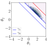
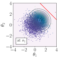
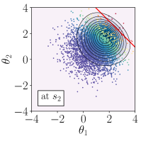
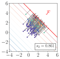
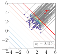
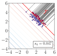
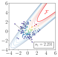
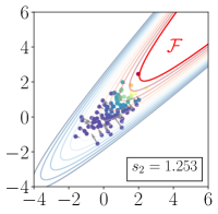
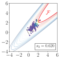
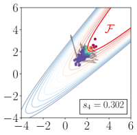
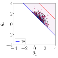
A comparison between the intermediate optimal biasing densities in CE and iCE is shown in Fig. 1.

CE method                                                      iCE method
Refer to caption Refer to caption Refer to caption Refer to caption

Figure 1: Samples and contours of the intermediate optimal biasing densities at two initial simulation levels (d=2𝑑2d=2). The standard CE method uses only Nρ𝑁𝜌N\cdot\rho elite weighted samples. The iCE method uses all N𝑁N weighted samples. The red solid line marks the target failure level and the color of the samples represents their weights.

3 Construction of the failure-informed subspace

As described in Section 2.1, the probability of failure psubscript𝑝p_{\mathcal{F}} and indicator 𝟙(𝜽)subscript1𝜽{\mathds{1}_{\mathcal{F}}\!\left(\bm{\theta}\right)} are analogous to the model evidence and likelihood function in Bayesian inference; thus, rare event simulation can be interpreted as a Bayesian inverse problem. Several dimension reduction techniques are available for nonlinear Bayesian inference [10, 11, 47]. The idea is to identify a certain low-dimensional structure in the parameter space, corresponding to the parameter directions along which the posterior differs most strongly from the prior. Particularly, the certified dimension reduction (CDR) approach [47] can be applied to any type of measurable likelihood function, as long as the gradient of its natural logarithm is square integrable. CDR provides low-dimensional approximations that are equipped with certified error bounds (in the sense of the KL divergence). As a result, the approximation can be controlled by some user-defined threshold bounding the KL divergence from the exact to the approximated posterior. We build on the ideas of [47] to construct low-dimensional approximations of the posterior-failure distribution.

The indicator function 𝟙(𝜽)subscript1𝜽{\mathds{1}_{\mathcal{F}}\!\left(\bm{\theta}\right)} is upper semi-continuous and does not provide sufficient regularity to construct the certified approximation (ln𝟙(𝜽)subscript1𝜽\nabla\ln{\mathds{1}_{\mathcal{F}}\!\left(\bm{\theta}\right)} is not square-integrable). Hence, we use one of the smooth representations f(𝜽;s)𝑓𝜽𝑠f({\bm{\theta};s}) in Eq. 13, to express the posterior-failure density as πf(𝜽;s)πpr(𝜽)proportional-tosubscript𝜋𝑓𝜽𝑠subscript𝜋pr𝜽\pi_{\mathcal{F}}\propto f({\bm{\theta};s})\pi_{\text{pr}}(\bm{\theta}), with s0𝑠0s\to 0. The idea is to find a low-dimensional approximation π(r)superscriptsubscript𝜋𝑟{\pi}_{\mathcal{F}}^{(r)} such that,

(16) π(𝜽)π(r)(𝜽)(h𝐏r)(𝜽)πpr(𝜽),subscript𝜋𝜽superscriptsubscript𝜋𝑟𝜽proportional-tosubscript𝐏𝑟𝜽subscript𝜋pr𝜽\pi_{\mathcal{F}}(\bm{\theta})\approx\pi_{\mathcal{F}}^{(r)}(\bm{\theta})\propto(h\circ\mathbf{P}_{r})(\bm{\theta})\pi_{\text{pr}}(\bm{\theta}),

where h:d>0:superscript𝑑subscriptabsent0h:\mathbbm{R}^{d}\to\mathbbm{R}_{>0} is a profile function and the projector 𝐏rd×dsubscript𝐏𝑟superscript𝑑𝑑\mathbf{P}_{r}\in\mathbbm{R}^{d\times d} is a linear transformation such that 𝐏r2=𝐏rsuperscriptsubscript𝐏𝑟2subscript𝐏𝑟\mathbf{P}_{r}^{2}=\mathbf{P}_{r}, but not necessarily 𝐏r𝖳=𝐏rsuperscriptsubscript𝐏𝑟𝖳subscript𝐏𝑟\mathbf{P}_{r}^{\mathsf{T}}=\mathbf{P}_{r}; we can also define the complementary projector to 𝐏rsubscript𝐏𝑟\mathbf{P}_{r} as the matrix 𝐏=𝐈d𝐏rsubscript𝐏perpendicular-tosubscript𝐈𝑑subscript𝐏𝑟\mathbf{P}_{\perp}=\mathbf{I}_{d}-{\mathbf{P}_{r}}, which satisfies Im(𝐏)=Ker(𝐏r)Imsubscript𝐏perpendicular-toKersubscript𝐏𝑟\mathrm{Im}(\mathbf{P}_{\perp})=\mathrm{Ker}({\mathbf{P}_{r}}).

The profile function in Eq. 16 depends only on 𝐏r𝜽=𝜽rsubscript𝐏𝑟𝜽subscript𝜽𝑟\mathbf{P}_{r}\bm{\theta}=\bm{\theta}_{r}, which is defined on the failure-informed subspace (FIS) 𝚯r=Im(𝐏r)subscript𝚯𝑟Imsubscript𝐏𝑟\mathbf{\Theta}_{r}=\mathrm{Im}({\mathbf{P}_{r}}), and it is essentially constant along the complementary subspace (CS) 𝚯=Ker(𝐏r)subscript𝚯perpendicular-toKersubscript𝐏𝑟\mathbf{\Theta}_{\perp}=\mathrm{Ker}({\mathbf{P}_{r}}). As a result, if rdmuch-less-than𝑟𝑑r\ll d, the goal of the approximation Eq. 16 is to replace the high-dimensional smooth indicator by a function of fewer variables. In the following, we employ the ideas of [47] to describe how the profile function and projector are obtained.

3.1 Optimal profile function

For a fixed projector 𝐏rsubscript𝐏𝑟\mathbf{P}_{r}, f(𝜽;s)𝑓𝜽𝑠f(\bm{\theta};s) can be approximated by its average over all values of 𝜽𝜽\bm{\theta} that map to 𝜽r=𝐏r𝜽subscript𝜽𝑟subscript𝐏𝑟𝜽\bm{\theta}_{r}=\mathbf{P}_{r}\bm{\theta} [33]. This is the conditional expectation of the smooth indicator given the projector under the prior distribution [47]

(17) 𝔼πpr[f(𝜽;s)|𝐏r𝜽]=𝚯~f(𝐏r𝜽+𝚽𝝃;s)πpr(𝐏r𝜽+𝚽𝝃)𝚯~πpr(𝐏r𝜽+𝚽𝝃)d𝝃π(𝝃|𝐏r𝜽)d𝝃,subscript𝔼subscript𝜋prdelimited-[]conditional𝑓𝜽𝑠subscript𝐏𝑟𝜽subscriptsubscript~𝚯perpendicular-to𝑓subscript𝐏𝑟𝜽subscript𝚽perpendicular-tosubscript𝝃perpendicular-to𝑠subscriptsubscript𝜋prsubscript𝐏𝑟𝜽subscript𝚽perpendicular-tosubscript𝝃perpendicular-tosubscriptsubscript~𝚯perpendicular-tosubscript𝜋prsubscript𝐏𝑟𝜽subscript𝚽perpendicular-tosuperscriptsubscript𝝃perpendicular-todifferential-dsuperscriptsubscript𝝃perpendicular-to𝜋conditionalsubscript𝝃perpendicular-tosubscript𝐏𝑟𝜽differential-dsubscript𝝃perpendicular-to\mathds{E}_{{\pi}_{\text{pr}}}\!\left[{f(\bm{\theta};s)\;|\;\mathbf{P}_{r}\bm{\theta}}\right]=\int_{\widetilde{\mathbf{\Theta}}_{\perp}}f(\mathbf{P}_{r}\bm{\theta}+\mathbf{\Phi}_{\perp}\bm{\xi}_{\perp};s)\leavevmode\nobreak\ \underbrace{\dfrac{{\pi}_{\text{pr}}(\mathbf{P}_{r}\bm{\theta}+\mathbf{\Phi}_{\perp}\bm{\xi}_{\perp})}{\int_{\widetilde{\mathbf{\Theta}}_{\perp}}{\pi}_{\text{pr}}(\mathbf{P}_{r}\bm{\theta}+\mathbf{\Phi}_{\perp}\bm{\xi}_{\perp}^{\prime})\mathrm{d}\bm{\xi}_{\perp}^{\prime}}}_{\pi(\bm{\xi}_{\perp}\;|\;\mathbf{P}_{r}\bm{\theta})}\leavevmode\nobreak\ \mathrm{d}\bm{\xi}_{\perp},

where 𝝃𝚯~drsubscript𝝃perpendicular-tosubscript~𝚯perpendicular-tosuperscript𝑑𝑟\bm{\xi}_{\perp}\in\widetilde{\mathbf{\Theta}}_{\perp}\subseteq\mathbbm{R}^{d-r}, and the columns of 𝚽d×drsubscript𝚽perpendicular-tosuperscript𝑑𝑑𝑟\mathbf{\Phi}_{\perp}\in\mathbbm{R}^{d\times d-r} form a basis for Ker(𝐏r)Kersubscript𝐏𝑟\mathrm{Ker}({\mathbf{P}_{r}}).

The optimal profile function hsuperscripth^{\star} is obtained by minimizing the KL divergence between the exact πsubscript𝜋{\pi}_{\mathcal{F}} and approximated π(r)superscriptsubscript𝜋𝑟\pi_{\mathcal{F}}^{(r)} densities. We can use the conditional expectation Eq. 17 to define:

(18) π(r)𝔼πpr[f(𝜽;s)|𝐏r𝜽](h𝐏r)(𝜽)πpr(𝜽),proportional-tosuperscriptsubscript𝜋𝑟subscriptsubscript𝔼subscript𝜋prdelimited-[]conditional𝑓𝜽𝑠subscript𝐏𝑟𝜽superscriptsubscript𝐏𝑟𝜽subscript𝜋pr𝜽\pi_{\mathcal{F}}^{(r)\star}\propto\underbrace{\mathds{E}_{{\pi}_{\text{pr}}}\!\left[{f(\bm{\theta};s)\;|\;\mathbf{P}_{r}\bm{\theta}}\right]}_{(h^{\star}\circ\mathbf{P}_{r})(\bm{\theta})}\pi_{\text{pr}}(\bm{\theta}),

for which the relation, DKL(π||π(r))DKL(π||π(r))=DKL(π(r)||π(r))0D_{\text{KL}}({\pi}_{\mathcal{F}}||\pi_{\mathcal{F}}^{(r)})-D_{\text{KL}}({\pi}_{\mathcal{F}}||\pi_{\mathcal{F}}^{(r)\star})=D_{\text{KL}}(\pi_{\mathcal{F}}^{(r)\star}||\pi_{\mathcal{F}}^{(r)})\geq 0 holds (see, [47]). In particular, DKL(π||π(r))DKL(π||π(r))D_{\text{KL}}(\pi_{\mathcal{F}}||\pi_{\mathcal{F}}^{(r)})\geq D_{\text{KL}}({\pi}_{\mathcal{F}}||\pi_{\mathcal{F}}^{(r)\star}), and hence a profile function of the form (h𝐏r)(𝜽)=𝔼πpr[f(𝜽;s)|𝐏r𝜽]superscriptsubscript𝐏𝑟𝜽subscript𝔼subscript𝜋prdelimited-[]conditional𝑓𝜽𝑠subscript𝐏𝑟𝜽(h^{\star}\circ\mathbf{P}_{r})(\bm{\theta})=\mathds{E}_{{\pi}_{\text{pr}}}\!\left[{f(\bm{\theta};s)\;|\;\mathbf{P}_{r}\bm{\theta}}\right] is a minimizer of DKL(π||π(r))D_{\text{KL}}({\pi}_{\mathcal{F}}||\pi_{\mathcal{F}}^{(r)}).

3.2 Optimal projector

Consider a Gaussian prior density πpr(𝜽)exp(V(𝜽))proportional-tosubscript𝜋pr𝜽𝑉𝜽\pi_{\mathrm{pr}}(\bm{\theta})\propto\exp(-V(\bm{\theta})), where the function V(𝜽)=12(𝜽𝝁pr)𝖳𝚺pr1(𝜽𝝁pr)𝑉𝜽12superscript𝜽subscript𝝁pr𝖳superscriptsubscript𝚺pr1𝜽subscript𝝁prV(\bm{\theta})\allowbreak=\frac{1}{2}(\bm{\theta}-\bm{\mu}_{\text{pr}})^{\mathsf{T}}\mathbf{\Sigma}_{\text{pr}}^{-1}(\bm{\theta}-\bm{\mu}_{\text{pr}}) is twice differentiable and satisfies 2V(𝜽)=𝚺pr1c𝐈dsuperscript2𝑉𝜽superscriptsubscript𝚺pr1succeeds-or-equals𝑐subscript𝐈𝑑\nabla^{2}V(\bm{\theta})=\mathbf{\Sigma}_{\text{pr}}^{-1}\succeq c\cdot\mathbf{I}_{d}, with c>0𝑐0c>0. Theorem 1 in [47] shows that, for any continuously differentiable function h:d:superscript𝑑h:\mathbbm{R}^{d}\to\mathbbm{R}, such that 𝔼πpr[h(𝜽)𝚺pr2]<subscript𝔼subscript𝜋prdelimited-[]superscriptsubscriptnorm𝜽subscript𝚺pr2\mathds{E}_{\pi_{\mathrm{pr}}}[\left\|\nabla h(\bm{\theta})\right\|_{\mathbf{\Sigma}_{\text{pr}}}^{2}]<\infty, the following subspace logarithmic Sobolev inequality holds

(19) 𝔼πpr[h2(𝜽)ln(h2(𝜽)𝔼πpr[h2(𝜽)|𝐏r𝜽])]subscript𝔼subscript𝜋prdelimited-[]superscript2𝜽superscript2𝜽subscript𝔼subscript𝜋prdelimited-[]conditionalsuperscript2𝜽subscript𝐏𝑟𝜽\displaystyle\mathds{E}_{\pi_{\mathrm{pr}}}\!\left[{h^{2}(\bm{\theta})\ln\left(\frac{h^{2}(\bm{\theta})}{\mathds{E}_{\pi_{\mathrm{pr}}}\!\left[{h^{2}(\bm{\theta})\;|\;\mathbf{P}_{r}\bm{\theta}}\right]}\right)}\right] 2𝔼πpr[(𝐈d𝐏r𝖳)h(𝜽)𝚺pr2],absent2subscript𝔼subscript𝜋prdelimited-[]superscriptsubscriptnormsubscript𝐈𝑑superscriptsubscript𝐏𝑟𝖳𝜽subscript𝚺pr2\displaystyle\leq 2\mathds{E}_{\pi_{\mathrm{pr}}}\!\left[{\left\|(\mathbf{I}_{d}-\mathbf{P}_{r}^{\mathsf{T}})\nabla h(\bm{\theta})\right\|_{\mathbf{\Sigma}_{\text{pr}}}^{2}}\right],

with the notation h(𝜽)𝚺pr2=h(𝜽)𝖳𝚺prh(𝜽)superscriptsubscriptnorm𝜽subscript𝚺pr2superscript𝜽𝖳subscript𝚺pr𝜽\left\|\nabla h(\bm{\theta})\right\|_{\mathbf{\Sigma}_{\text{pr}}}^{2}=\nabla h(\bm{\theta})^{\mathsf{T}}\mathbf{\Sigma}_{\text{pr}}\nabla h(\bm{\theta}). The inequality Eq. 19 allows one to bound DKL(π||π(r))D_{\text{KL}}({\pi}_{\mathcal{F}}||\pi_{\mathcal{F}}^{(r)\star}), which in turn provides a way to characterize the optimal projector in the approximation π(r)superscriptsubscript𝜋𝑟\pi_{\mathcal{F}}^{(r)\star} of Eq. 18.

Let h2(𝜽)superscript2𝜽h^{2}(\bm{\theta}) be equal to the normalized smooth indicator function f(𝜽;s)/p𝑓𝜽𝑠𝑝f(\bm{\theta};s)/p, such that h(𝜽)=12(f(𝜽;s)/p)1/2lnf(𝜽;s)𝜽12superscript𝑓𝜽𝑠𝑝12𝑓𝜽𝑠\nabla h(\bm{\theta})=\frac{1}{2}(f(\bm{\theta};s)/p)^{\nicefrac{{1}}{{2}}}\nabla\ln f(\bm{\theta};s); then Eq. 19 becomes

(20) 𝔼πpr[f(𝜽;s)pln(f(𝜽;s)/p𝔼πpr[f(𝜽;s)|𝐏r𝜽]/p)]subscript𝔼subscript𝜋prdelimited-[]𝑓𝜽𝑠𝑝𝑓𝜽𝑠𝑝subscript𝔼subscript𝜋prdelimited-[]conditional𝑓𝜽𝑠subscript𝐏𝑟𝜽subscript𝑝\displaystyle\mathds{E}_{\pi_{\mathrm{pr}}}\!\left[{\frac{f(\bm{\theta};s)}{p}\ln\left(\frac{f(\bm{\theta};s)/p}{\mathds{E}_{\pi_{\mathrm{pr}}}\!\left[{f(\bm{\theta};s)\;|\;\mathbf{P}_{r}\bm{\theta}}\right]/p_{\mathcal{F}}}\right)}\right] 12𝔼πpr[f(𝜽;s)p(𝐈d𝐏r𝖳)lnf(𝜽;s)𝚺pr2].absent12subscript𝔼subscript𝜋prdelimited-[]𝑓𝜽𝑠𝑝superscriptsubscriptnormsubscript𝐈𝑑superscriptsubscript𝐏𝑟𝖳𝑓𝜽𝑠subscript𝚺pr2\displaystyle\leq\frac{1}{2}\leavevmode\nobreak\ \mathds{E}_{\pi_{\mathrm{pr}}}\!\left[{\frac{f(\bm{\theta};s)}{p}\left\|(\mathbf{I}_{d}-\mathbf{P}_{r}^{\mathsf{T}})\nabla\ln f(\bm{\theta};s)\right\|_{\mathbf{\Sigma}_{\text{pr}}}^{2}}\right].

The left-hand side in Eq. 20 is equal to DKL(π||π(r))D_{\text{KL}}({\pi}_{\mathcal{F}}||\pi_{\mathcal{F}}^{(r)\star}); hence we obtain the bound

DKL(π||π(r))\displaystyle{D}_{\text{KL}}\left({\pi}_{\mathcal{F}}||\pi_{\mathcal{F}}^{(r)\star}\right) 12𝔼π[(𝐈d𝐏r𝖳)lnf(𝜽;s)𝚺pr2]absent12subscript𝔼subscript𝜋delimited-[]superscriptsubscriptnormsubscript𝐈𝑑superscriptsubscript𝐏𝑟𝖳𝑓𝜽𝑠subscript𝚺pr2\displaystyle\leq\frac{1}{2}\leavevmode\nobreak\ \mathds{E}_{\pi_{\mathcal{F}}}\!\left[{\left\|(\mathbf{I}_{d}-\mathbf{P}_{r}^{\mathsf{T}})\nabla\ln f(\bm{\theta};s)\right\|_{\mathbf{\Sigma}_{\text{pr}}}^{2}}\right]
=12𝔼π[tr(𝚺pr(𝐈d𝐏r𝖳)lnf(𝜽;s)lnf(𝜽;s)𝖳(𝐈d𝐏r))]absent12subscript𝔼subscript𝜋delimited-[]trsubscript𝚺prsubscript𝐈𝑑superscriptsubscript𝐏𝑟𝖳𝑓𝜽𝑠𝑓superscript𝜽𝑠𝖳subscript𝐈𝑑subscript𝐏𝑟\displaystyle=\frac{1}{2}\leavevmode\nobreak\ \mathds{E}_{\pi_{\mathcal{F}}}\!\left[{\mathrm{tr}\left(\mathbf{\Sigma}_{\text{pr}}(\mathbf{I}_{d}-\mathbf{P}_{r}^{\mathsf{T}})\nabla\ln f(\bm{\theta};s)\nabla\ln f(\bm{\theta};s)^{\mathsf{T}}(\mathbf{I}_{d}-\mathbf{P}_{r})\right)}\right]
(21) =12tr(𝚺pr(𝐈d𝐏r𝖳)𝐇(𝐈d𝐏r))12(𝐏r,𝐇),absent12trsubscript𝚺prsubscript𝐈𝑑superscriptsubscript𝐏𝑟𝖳𝐇subscript𝐈𝑑subscript𝐏𝑟12subscript𝐏𝑟𝐇\displaystyle=\frac{1}{2}\leavevmode\nobreak\ \mathrm{tr}\left(\mathbf{\Sigma}_{\text{pr}}(\mathbf{I}_{d}-\mathbf{P}_{r}^{\mathsf{T}})\leavevmode\nobreak\ \mathbf{H}\leavevmode\nobreak\ (\mathbf{I}_{d}-\mathbf{P}_{r})\right)\eqqcolon\frac{1}{2}\leavevmode\nobreak\ \mathcal{R}(\mathbf{P}_{r},\mathbf{H}),

where (𝐏r,𝐇)subscript𝐏𝑟𝐇\mathcal{R}(\mathbf{P}_{r},\mathbf{H}) is the mean-squared error of the approximation of lnf(𝜽;s)𝑓𝜽𝑠\nabla\ln f(\bm{\theta};s) by 𝐏r𝖳lnf(𝜽;s)superscriptsubscript𝐏𝑟𝖳𝑓𝜽𝑠\mathbf{P}_{r}^{\mathsf{T}}\nabla\ln f(\bm{\theta};s) (with the parameter 𝜽πsimilar-to𝜽subscript𝜋\bm{\theta}\sim\pi_{\mathcal{F}}), and 𝐇d×d𝐇superscript𝑑𝑑\mathbf{H}\in\mathbbm{R}^{d\times d} is the second moment matrix of the gradient of the log-smooth indicator function [47]

(22) 𝐇=𝚯lnf(𝜽;s)lnf(𝜽;s)𝖳π(𝜽)d𝜽=𝔼π[lnf(𝜽;s)lnf(𝜽;s)𝖳].𝐇subscript𝚯𝑓𝜽𝑠𝑓superscript𝜽𝑠𝖳subscript𝜋𝜽differential-d𝜽subscript𝔼subscript𝜋delimited-[]𝑓𝜽𝑠𝑓superscript𝜽𝑠𝖳\mathbf{H}=\int_{\mathbf{\Theta}}\nabla\ln f(\bm{\theta};s)\nabla\ln f(\bm{\theta};s)^{\mathsf{T}}{\pi}_{\mathcal{F}}(\bm{\theta})\mathrm{d}\bm{\theta}=\mathds{E}_{{\pi}_{\mathcal{F}}}\!\left[{\nabla\ln f(\bm{\theta};s)\nabla\ln f(\bm{\theta};s)^{\mathsf{T}}}\right].

Note from Eq. 21 that the mean-squared error is quadratic in 𝐏rsubscript𝐏𝑟\mathbf{P}_{r}. Therefore, one can minimize the upper bound in Eq. 21 over the collection of r𝑟r-rank projectors to find an optimal projector:

(23) 𝐏r=argmin𝐏rd×d(𝐏r,𝐇).subscript𝐏𝑟subscriptargminsuperscriptsubscript𝐏𝑟superscript𝑑𝑑superscriptsubscript𝐏𝑟𝐇\mathbf{P}_{r}=\operatorname*{arg\,min}_{\mathbf{P}_{r}^{\prime}\in\mathbbm{R}^{d\times d}}\mathcal{R}(\mathbf{P}_{r}^{\prime},\mathbf{H}).

As shown by Proposition 2 in [47], a solution to Eq. 23 is

(24) 𝐏r=(i=1rϕiϕi𝖳)𝚺pr1andmin(𝐏r,𝐇)=i=r+1dλi,formulae-sequencesubscript𝐏𝑟superscriptsubscript𝑖1𝑟subscriptbold-italic-ϕ𝑖superscriptsubscriptbold-italic-ϕ𝑖𝖳superscriptsubscript𝚺pr1andsubscript𝐏𝑟𝐇superscriptsubscript𝑖𝑟1𝑑subscript𝜆𝑖\mathbf{P}_{r}=\left(\sum_{i=1}^{r}\bm{\phi}_{i}\bm{\phi}_{i}^{\mathsf{T}}\right)\mathbf{\Sigma}_{\text{pr}}^{-1}\qquad\mathrm{and}\qquad\min\mathcal{R}(\mathbf{P}_{r},\mathbf{H})=\sum_{i=r+1}^{d}\lambda_{i},

where the eigenpairs (λi,ϕi)subscript𝜆𝑖subscriptbold-italic-ϕ𝑖(\lambda_{i},\bm{\phi}_{i}) correspond to the solution of the generalized eigenvalue problem 𝐇ϕi=λi𝚺pr1ϕi,i=1,,dformulae-sequence𝐇subscriptbold-italic-ϕ𝑖subscript𝜆𝑖superscriptsubscript𝚺pr1subscriptbold-italic-ϕ𝑖𝑖1𝑑\mathbf{H}\bm{\phi}_{i}=\lambda_{i}\mathbf{\Sigma}_{\text{pr}}^{-1}\bm{\phi}_{i},\leavevmode\nobreak\ i=1,\ldots,d. Hence, if πprsubscript𝜋pr\pi_{\mathrm{pr}} satisfies the inequality Eq. 19 and 𝐏rsubscript𝐏𝑟\mathbf{P}_{r} is defined as in Eq. 24, the approximation π(r)superscriptsubscript𝜋𝑟\pi_{\mathcal{F}}^{(r)\star} in Eq. 18 can be controlled by a desired tolerance ε0𝜀0\varepsilon\geq 0 as

(25) DKL(π||π(r))12i=r+1dλiε.{D}_{\text{KL}}\left({\pi}_{\mathcal{F}}||\pi_{\mathcal{F}}^{(r)\star}\right)\leq\frac{1}{2}\sum_{i=r+1}^{d}\lambda_{i}\leq\varepsilon.

In this case, bounding DKL(π||π(r))D_{\text{KL}}({\pi}_{\mathcal{F}}||\pi_{\mathcal{F}}^{(r)\star}) amounts to selecting the rank r𝑟r as the smallest integer such that the left-hand side of Eq. 25 is below a prescribed ε𝜀\varepsilon, i.e., r=min{r:12i=r+1dλiε}𝑟:superscript𝑟12superscriptsubscript𝑖superscript𝑟1𝑑subscript𝜆𝑖𝜀r=\min\left\{r^{\prime}:\frac{1}{2}\sum_{i=r^{\prime}+1}^{d}\lambda_{i}\leq\varepsilon\right\}. Note that, along with the prior, the second-moment matrix of the log-smooth indicator function 𝐇𝐇\mathbf{H} reveals the effective low dimension of the posterior-failure distribution. A sharp decay in the generalized spectrum of (𝐇,𝚺pr1)𝐇superscriptsubscript𝚺pr1(\mathbf{H},\mathbf{\Sigma}_{\text{pr}}^{-1}) guarantees the existence of a low-rank approximation rdmuch-less-than𝑟𝑑r\ll d.

4 Failure-informed cross-entropy-based importance sampling

As shown in Section 2.2, the optimal IS biasing density πbiassubscriptsuperscript𝜋bias\pi^{\star}_{\text{bias}} is equivalent to the posterior-failure density πsubscript𝜋\pi_{\mathcal{F}}. Hence, we can employ the theory of Section 3 to derive low-dimensional biasing distributions that extend the application of the iCE method to high-dimensional parameter spaces that have an intrinsic low-dimensional structure. Recall that the goal is to represent π(𝜽)=πbias(𝜽)f(𝜽;s)πpr(𝜽)subscript𝜋𝜽superscriptsubscript𝜋bias𝜽proportional-to𝑓𝜽𝑠subscript𝜋pr𝜽\pi_{\mathcal{F}}(\bm{\theta})={\pi}_{\text{bias}}^{\star}(\bm{\theta})\propto f(\bm{\theta};s)\pi_{\text{pr}}(\bm{\theta}) (as s0𝑠0s\to 0) on the FIS using the certified approximation Eq. 18.

4.1 Formulation

Based on remark 2.1, we can impose that the prior πpr(𝜽)subscript𝜋pr𝜽\pi_{\text{pr}}(\bm{\theta}) is standard Gaussian. The solution of the generalized eigenvalue problem (𝐇,𝚺pr1)𝐇superscriptsubscript𝚺pr1(\mathbf{H},\mathbf{\Sigma}_{\mathrm{pr}}^{-1}) required for the construction of 𝐏rsubscript𝐏𝑟\mathbf{P}_{r} in Eq. 24, reduces to a standard eigenvalue problem for 𝐇𝐇\mathbf{H}. As a result, the projector can be written as 𝐏r=𝚽r𝚽r𝖳subscript𝐏𝑟subscript𝚽𝑟superscriptsubscript𝚽𝑟𝖳\mathbf{P}_{r}=\mathbf{\Phi}_{r}\mathbf{\Phi}_{r}^{\mathsf{T}}, where 𝚽rd×rsubscript𝚽𝑟superscript𝑑𝑟\mathbf{\Phi}_{r}\in\mathbbm{R}^{d\times r} contains the first r𝑟r eigenvectors defining a basis for the FIS. Similarly, the complementary projector can be obtained as 𝐏=𝚽𝚽𝖳subscript𝐏perpendicular-tosubscript𝚽perpendicular-tosuperscriptsubscript𝚽perpendicular-to𝖳\mathbf{P}_{\perp}=\mathbf{\Phi}_{\perp}\mathbf{\Phi}_{\perp}^{\mathsf{T}}, where 𝚽d×drsubscript𝚽perpendicular-tosuperscript𝑑𝑑𝑟\mathbf{\Phi}_{\perp}\in\mathbbm{R}^{d\times d-r} is defined by the remaining eigenvectors, generating a basis for the CS.

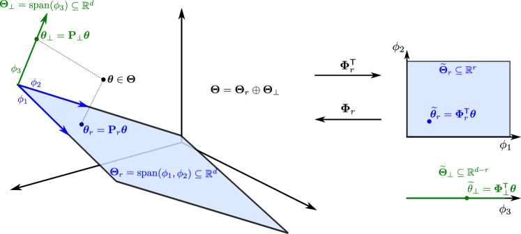
The projector 𝐏rsubscript𝐏𝑟\mathbf{P}_{r} is orthogonal with respect to the prior precision matrix 𝚺pr1=𝐈dsuperscriptsubscript𝚺pr1subscript𝐈𝑑\mathbf{\Sigma}_{\mathrm{pr}}^{-1}=\mathbf{I}_{d}. This induces a decomposition of the parameter space as the direct sum 𝚯=𝚯r𝚯𝚯direct-sumsubscript𝚯𝑟subscript𝚯perpendicular-to{\bm{\Theta}}={\bm{\Theta}}_{r}\oplus{\bm{\Theta}}_{\perp}, where any element of 𝚯𝚯{\bm{\Theta}} can be uniquely represented as 𝜽=𝜽r+𝜽𝜽subscript𝜽𝑟subscript𝜽perpendicular-to\bm{\theta}=\bm{\theta}_{r}+\bm{\theta}_{\perp}, with 𝜽r=𝐏r𝜽𝚯rsubscript𝜽𝑟subscript𝐏𝑟𝜽subscript𝚯𝑟\bm{\theta}_{r}=\mathbf{P}_{r}\bm{\theta}\in\bm{\Theta}_{r} and 𝜽=𝐏𝜽𝚯subscript𝜽perpendicular-tosubscript𝐏perpendicular-to𝜽subscript𝚯perpendicular-to\bm{\theta}_{\perp}=\mathbf{P}_{\perp}\bm{\theta}\in\bm{\Theta}_{\perp}. Moreover, we can use the operators 𝚽rsubscript𝚽𝑟\mathbf{\Phi}_{r} and 𝚽subscript𝚽perpendicular-to\mathbf{\Phi}_{\perp} to map the parameters onto a local FIS 𝚯~rrsubscript~𝚯𝑟superscript𝑟\widetilde{\mathbf{\Theta}}_{r}\subseteq\mathbbm{R}^{r} and local CS 𝚯~drsubscript~𝚯perpendicular-tosuperscript𝑑𝑟\widetilde{\mathbf{\Theta}}_{\perp}\subseteq\mathbbm{R}^{d-r}, respectively. In this case, the parameter vector can be written as 𝜽=𝚽r𝜽~r+𝚽𝜽~𝜽subscript𝚽𝑟subscript~𝜽𝑟subscript𝚽perpendicular-tosubscript~𝜽perpendicular-to\bm{\theta}=\mathbf{\Phi}_{r}\widetilde{\bm{\theta}}_{r}+\mathbf{\Phi}_{\perp}\widetilde{\bm{\theta}}_{\perp}, where 𝜽~=[𝜽~r,𝜽~]~𝜽subscript~𝜽𝑟subscript~𝜽perpendicular-to\widetilde{\bm{\theta}}=[\widetilde{\bm{\theta}}_{r},\widetilde{\bm{\theta}}_{\perp}] has components 𝜽~r=𝚽r𝖳𝜽𝚯~rsubscript~𝜽𝑟superscriptsubscript𝚽𝑟𝖳𝜽subscript~𝚯𝑟\widetilde{\bm{\theta}}_{r}=\mathbf{\Phi}_{r}^{\mathsf{T}}{\bm{\theta}}\in\widetilde{\mathbf{\Theta}}_{r} and 𝜽~=𝚽𝖳𝜽𝚯~subscript~𝜽perpendicular-tosuperscriptsubscript𝚽perpendicular-to𝖳𝜽subscript~𝚯perpendicular-to\widetilde{\bm{\theta}}_{\perp}=\mathbf{\Phi}_{\perp}^{\mathsf{T}}{\bm{\theta}}\in\widetilde{\mathbf{\Theta}}_{\perp}. Figure 2 illustrates the action of the projectors and basis operators.
Refer to caption
Figure 2: Schematic representation of a parameter 𝜽3𝜽superscript3\bm{\theta}\in\mathbbm{R}^{3} projected onto the FIS with r=2𝑟2r=2 (in blue): global 𝜽rdsubscript𝜽𝑟superscript𝑑{\bm{\theta}}_{r}\in\mathbbm{R}^{d}, local 𝜽~rrsubscript~𝜽𝑟superscript𝑟\widetilde{\bm{\theta}}_{r}\in\mathbbm{R}^{r} (adapted from [11]).

From the discussion above, we see that the prior distribution can be factorized as πpr(𝜽~)=πpr(r)(𝜽~r)πpr()(𝜽~)subscript𝜋pr~𝜽superscriptsubscript𝜋pr𝑟subscript~𝜽𝑟superscriptsubscript𝜋prperpendicular-tosubscript~𝜽perpendicular-to\pi_{\mathrm{pr}}(\widetilde{\bm{\theta}})=\pi_{\text{pr}}^{(r)}(\widetilde{\bm{\theta}}_{r}){\pi}_{\text{pr}}^{(\perp)}(\widetilde{\bm{\theta}}_{\perp}), where πpr(r)(𝜽~r)superscriptsubscript𝜋pr𝑟subscript~𝜽𝑟\pi_{\text{pr}}^{(r)}(\widetilde{\bm{\theta}}_{r}) and πpr()(𝜽~)superscriptsubscript𝜋prperpendicular-tosubscript~𝜽perpendicular-to{\pi}_{\text{pr}}^{(\perp)}(\widetilde{\bm{\theta}}_{\perp}) are densities on the local FIS and CS, respectively [11]. This choice, together with the certified approximation in Eq. 18, allows us to define the optimal low-dimensional biasing density:

(26) π(r)(𝜽~)=πbias(𝜽~)𝔼πpr[f(𝜽;s)|𝚽r𝜽~r]πpr(r)(𝜽~r)reduced optimal biasingπpr()(𝜽~).complementary prior{\pi}_{\mathcal{F}}^{(r)\star}(\widetilde{\bm{\theta}})={\pi}_{\text{bias}}^{\star}(\widetilde{\bm{\theta}})\propto\underbrace{\mathds{E}_{{\pi}_{\text{pr}}}\!\left[{f(\bm{\theta};s)\;|\;\bm{\Phi}_{r}\widetilde{\bm{\theta}}_{r}}\right]\leavevmode\nobreak\ {\pi}_{\text{pr}}^{(r)}(\widetilde{\bm{\theta}}_{r})}_{\text{reduced optimal biasing}}\leavevmode\nobreak\ \underbrace{{\pi}_{\text{pr}}^{(\perp)}(\widetilde{\bm{\theta}}_{\perp}).}_{\text{complementary prior}}

We select the parametric biasing distribution from a Gaussian family that decomposes as follows:

(27) πbias(𝜽~;𝝊r)=πbias(r)(𝜽~r;𝝊r)πpr()(𝜽~);subscript𝜋bias~𝜽subscript𝝊𝑟superscriptsubscript𝜋bias𝑟subscript~𝜽𝑟subscript𝝊𝑟superscriptsubscript𝜋prperpendicular-tosubscript~𝜽perpendicular-to{\pi}_{\text{bias}}(\widetilde{\bm{\theta}};\bm{\upsilon}_{r})={\pi}_{\text{bias}}^{(r)}(\widetilde{\bm{\theta}}_{r};\bm{\upsilon}_{r})\leavevmode\nobreak\ {\pi}_{\text{pr}}^{(\perp)}(\widetilde{\bm{\theta}}_{\perp});

this family has a general Gaussian form on the local FIS, where 𝝊rΥrsubscript𝝊𝑟subscriptΥ𝑟\bm{\upsilon}_{r}\in\Upsilon_{r} represents the mean and covariance matrix of the r𝑟r-dimensional reduced Gaussian density, and is equal to the standard Gaussian prior in the complementary directions.

Aiming at the optimal biasing density Eq. 26 using biasing densities of the form Eq. 27, the CE optimization problem can be re-defined on a low-dimensional space. The KL divergence between Eq. 26 and Eq. 27 reads

(28) DKL(πbias||πbias)=𝔼πbias[ln(p1𝔼πpr[f(𝜽;s)|𝚽r𝜽~r]πpr(r)(𝜽~r)πbias(r)(𝜽~r;𝝊r))].{D}_{\text{KL}}\left(\pi_{\text{bias}}^{\star}||{\pi}_{\text{bias}}\right)=\mathds{E}_{\pi_{\text{bias}}^{\star}}\!\left[{\ln\left(\dfrac{p_{\mathcal{F}}^{-1}\mathds{E}_{{\pi}_{\text{pr}}}\!\left[{f(\bm{\theta};s)\;|\;\mathbf{\Phi}_{r}\widetilde{\bm{\theta}}_{r}}\right]\leavevmode\nobreak\ {\pi}_{\text{pr}}^{(r)}(\widetilde{\bm{\theta}}_{r})}{{\pi}_{\text{bias}}^{(r)}(\widetilde{\bm{\theta}}_{r};\bm{\upsilon}_{r})}\right)}\right].

As in Section 2.3, minimizing DKL(πbias||πbias)D_{\text{KL}}(\pi_{\text{bias}}^{\star}||{\pi}_{\text{bias}}) is equivalent to the following maximization:

𝝊rsubscriptsuperscript𝝊𝑟\displaystyle\bm{\upsilon}^{\star}_{r} =argmax𝝊rΥr𝔼πbias[lnπbias(r)(𝜽~r;𝝊r)]absentsubscriptargmaxsubscript𝝊𝑟subscriptΥ𝑟subscript𝔼superscriptsubscript𝜋biasdelimited-[]superscriptsubscript𝜋bias𝑟subscript~𝜽𝑟subscript𝝊𝑟\displaystyle=\operatorname*{arg\,max}_{\bm{\upsilon}_{r}\in\Upsilon_{r}}\mathds{E}_{\pi_{\text{bias}}^{\star}}\!\left[{\ln{\pi}_{\text{bias}}^{(r)}(\widetilde{\bm{\theta}}_{r};\bm{\upsilon}_{r})}\right]
=argmax𝝊rΥr𝚯~r𝚯~lnπbias(r)(𝜽~r;𝝊r)𝔼πpr[f(𝜽;s)|𝚽r𝜽~r]πpr(r)(𝜽~r)πpr()(𝜽~)d𝜽~d𝜽~rabsentsubscriptargmaxsubscript𝝊𝑟subscriptΥ𝑟subscriptsubscript~𝚯𝑟subscriptsubscript~𝚯perpendicular-tosuperscriptsubscript𝜋bias𝑟subscript~𝜽𝑟subscript𝝊𝑟subscript𝔼subscript𝜋prdelimited-[]conditional𝑓𝜽𝑠subscript𝚽𝑟subscript~𝜽𝑟superscriptsubscript𝜋pr𝑟subscript~𝜽𝑟superscriptsubscript𝜋prperpendicular-tosubscript~𝜽perpendicular-todifferential-dsubscript~𝜽perpendicular-todifferential-dsubscript~𝜽𝑟\displaystyle=\operatorname*{arg\,max}_{\bm{\upsilon}_{r}\in\Upsilon_{r}}\int_{\widetilde{\mathbf{\Theta}}_{r}}\int_{\widetilde{\mathbf{\Theta}}_{\perp}}\ln{\pi}_{\text{bias}}^{(r)}(\widetilde{\bm{\theta}}_{r};\bm{\upsilon}_{r})\mathds{E}_{{\pi}_{\text{pr}}}\!\left[{f(\bm{\theta};s)\;|\;\bm{\Phi}_{r}\widetilde{\bm{\theta}}_{r}}\right]\leavevmode\nobreak\ {\pi}_{\text{pr}}^{(r)}(\widetilde{\bm{\theta}}_{r}){\pi}_{\text{pr}}^{(\perp)}(\widetilde{\bm{\theta}}_{\perp})\mathrm{d}\widetilde{\bm{\theta}}_{\perp}\mathrm{d}\widetilde{\bm{\theta}}_{r}
=argmax𝝊rΥr𝚯~r[𝚯~f(𝚽r𝜽~r+𝚽𝝃~;s)πpr()(𝝃~)d𝝃~]lnπbias(r)(𝜽~r;𝝊r)πpr(r)(𝜽~r)d𝜽~rabsentsubscriptargmaxsubscript𝝊𝑟subscriptΥ𝑟subscriptsubscript~𝚯𝑟delimited-[]subscriptsubscript~𝚯perpendicular-to𝑓subscript𝚽𝑟subscript~𝜽𝑟subscript𝚽perpendicular-tosubscript~𝝃perpendicular-to𝑠superscriptsubscript𝜋prperpendicular-tosubscript~𝝃perpendicular-todifferential-dsubscript~𝝃perpendicular-tosuperscriptsubscript𝜋bias𝑟subscript~𝜽𝑟subscript𝝊𝑟superscriptsubscript𝜋pr𝑟subscript~𝜽𝑟differential-dsubscript~𝜽𝑟\displaystyle=\operatorname*{arg\,max}_{\bm{\upsilon}_{r}\in\Upsilon_{r}}\int_{\widetilde{\mathbf{\Theta}}_{r}}\left[\int_{\widetilde{\mathbf{\Theta}}_{\perp}}f(\mathbf{\Phi}_{r}\widetilde{\bm{\theta}}_{r}+\mathbf{\Phi}_{\perp}\widetilde{\bm{\xi}}_{\perp};s)\leavevmode\nobreak\ {\pi}_{\text{pr}}^{(\perp)}(\widetilde{\bm{\xi}}_{\perp})\mathrm{d}\widetilde{\bm{\xi}}_{\perp}\right]\ln{\pi}_{\text{bias}}^{(r)}(\widetilde{\bm{\theta}}_{r};\bm{\upsilon}_{r})\pi_{\text{pr}}^{(r)}(\widetilde{\bm{\theta}}_{r})\mathrm{d}\widetilde{\bm{\theta}}_{r}
(29) =argmax𝝊rΥr𝔼πpr[f(𝚽r𝜽~r+𝚽𝜽~;s)lnπbias(r)(𝜽~r;𝝊r)].absentsubscriptargmaxsubscript𝝊𝑟subscriptΥ𝑟subscript𝔼subscript𝜋prdelimited-[]𝑓subscript𝚽𝑟subscript~𝜽𝑟subscript𝚽perpendicular-tosubscript~𝜽perpendicular-to𝑠superscriptsubscript𝜋bias𝑟subscript~𝜽𝑟subscript𝝊𝑟\displaystyle=\operatorname*{arg\,max}_{\bm{\upsilon}_{r}\in\Upsilon_{r}}\mathds{E}_{\pi_{\text{pr}}}\!\left[{f(\mathbf{\Phi}_{r}\widetilde{\bm{\theta}}_{r}+\mathbf{\Phi}_{\perp}\widetilde{\bm{\theta}}_{\perp};s)\ln{\pi}_{\text{bias}}^{(r)}(\widetilde{\bm{\theta}}_{r};\bm{\upsilon}_{r})}\right].

Note that in this CE formulation there is no need for evaluating the conditional expectation in Eq. 26, as it is normally the case when applying sequential IS in the Bayesian inference setting where Markov chain Monte Carlo techniques are required to draw samples from Eq. 26 (see, e.g., [11, 47]). Indeed, only an expectation with respect to the full prior density is required, thus avoiding the computational demands associated with double-loop procedures.

Instead of directly taking the expectation with respect to the prior in Eq. 29, we apply IS with biasing distribution πbias(𝜽~;𝝊r)subscript𝜋bias~𝜽subscriptsuperscript𝝊𝑟{\pi}_{\text{bias}}(\widetilde{\bm{\theta}};\bm{\upsilon}^{\prime}_{r}) in Eq. 27:

(30) 𝝊r=argmax𝝊rΥr𝔼πbias(;𝝊r)[f(𝚽r𝜽~r+𝚽𝜽~;s)lnπbias(r)(𝜽~r;𝝊r)πpr(𝜽~)πbias(𝜽~;𝝊r)]subscriptsuperscript𝝊𝑟subscriptargmaxsubscript𝝊𝑟subscriptΥ𝑟subscript𝔼subscript𝜋biassuperscriptsubscript𝝊𝑟delimited-[]𝑓subscript𝚽𝑟subscript~𝜽𝑟subscript𝚽perpendicular-tosubscript~𝜽perpendicular-to𝑠superscriptsubscript𝜋bias𝑟subscript~𝜽𝑟subscript𝝊𝑟subscript𝜋pr~𝜽subscript𝜋bias~𝜽superscriptsubscript𝝊𝑟\bm{\upsilon}^{\star}_{r}=\operatorname*{arg\,max}_{\bm{\upsilon}_{r}\in\Upsilon_{r}}\mathds{E}_{{\pi}_{\text{bias}}(\cdot;\bm{\upsilon}_{r}^{\prime})}\!\left[{f(\mathbf{\Phi}_{r}\widetilde{\bm{\theta}}_{r}+\mathbf{\Phi}_{\perp}\widetilde{\bm{\theta}}_{\perp};s)\ln{\pi}_{\text{bias}}^{(r)}(\widetilde{\bm{\theta}}_{r};\bm{\upsilon}_{r})\leavevmode\nobreak\ \dfrac{\pi_{\text{pr}}(\widetilde{\bm{\theta}})}{{\pi}_{\mathrm{bias}}(\widetilde{\bm{\theta}};\bm{\upsilon}_{r}^{\prime})}}\right]

for reference parameters 𝝊rsubscriptsuperscript𝝊𝑟\bm{\upsilon}^{\prime}_{r}. We apply the IS estimator of the expectation Eq. 30 to define the stochastic optimization problem:

(31) 𝝊r𝝊^r=argmax𝝊rΥr1Ni=1Nf(𝚽r𝜽~r,i+𝚽𝜽~,i;s)lnπbias(r)(𝜽~r,i;𝝊r)w(𝜽~i;𝝊r)superscriptsubscript𝝊𝑟superscriptsubscript^𝝊𝑟subscriptargmaxsubscript𝝊𝑟subscriptΥ𝑟1𝑁superscriptsubscript𝑖1𝑁𝑓subscript𝚽𝑟subscript~𝜽𝑟𝑖subscript𝚽perpendicular-tosubscript~𝜽perpendicular-to𝑖𝑠superscriptsubscript𝜋bias𝑟subscript~𝜽𝑟𝑖subscript𝝊𝑟𝑤subscript~𝜽𝑖subscriptsuperscript𝝊𝑟{\bm{\upsilon}}_{r}^{\star}\approx\widehat{\bm{\upsilon}}_{r}^{\star}=\operatorname*{arg\,max}_{\bm{\upsilon}_{r}\in\Upsilon_{r}}\dfrac{1}{N}\sum_{i=1}^{N}f\left(\mathbf{\Phi}_{r}\widetilde{\bm{\theta}}_{r,i}+\mathbf{\Phi}_{\perp}\widetilde{\bm{\theta}}_{\perp,i};s\right)\ln{\pi}_{\text{bias}}^{(r)}\left(\widetilde{\bm{\theta}}_{r,i};\bm{\upsilon}_{r}\right)w\left(\widetilde{\bm{\theta}}_{i};\bm{\upsilon}^{\prime}_{r}\right)

where {𝜽~i=[𝜽~r,i,𝜽~,i]}i=1Ni.i.d.πbias(;𝝊r)superscriptsubscriptsubscript~𝜽𝑖subscript~𝜽𝑟𝑖subscript~𝜽perpendicular-to𝑖𝑖1𝑁i.i.d.similar-tosubscript𝜋biassubscriptsuperscript𝝊𝑟\{\widetilde{\bm{\theta}}_{i}=[\widetilde{\bm{\theta}}_{r,i},\widetilde{\bm{\theta}}_{\perp,i}]\}_{i=1}^{N}\overset{\text{i.i.d.}}{\sim}{\pi}_{\text{bias}}(\cdot;\bm{\upsilon}^{\prime}_{r}) and w(𝜽~i;𝝊r)=πpr(𝜽~)/πbias(𝜽~;𝝊r)𝑤subscript~𝜽𝑖subscriptsuperscript𝝊𝑟subscript𝜋pr~𝜽subscript𝜋bias~𝜽superscriptsubscript𝝊𝑟w(\widetilde{\bm{\theta}}_{i};\bm{\upsilon}^{\prime}_{r})=\pi_{\text{pr}}(\widetilde{\bm{\theta}})/{\pi}_{\mathrm{bias}}(\widetilde{\bm{\theta}};\bm{\upsilon}_{r}^{\prime}). As in the iCE method, the optimization Eq. 31 is performed sequentially by introducing a set of smoothing parameters {sj>0}j=0nlvsuperscriptsubscriptsubscript𝑠𝑗0𝑗0subscript𝑛lv\{s_{j}>0\}_{j=0}^{n_{\text{lv}}}.

Starting in the full-dimensional space at level j=0𝑗0j=0, the iCE method applied to the FIS requires two main steps: (i) finding the projector and associated basis operators, and (ii) updating the reduced reference parameters 𝝊^r(j+1)superscriptsubscript^𝝊𝑟𝑗1\widehat{\bm{\upsilon}}_{r}^{(j+1)} of the next intermediate biasing density. To achieve both steps, we use samples from the current biasing density πbias(;𝝊^r(j))subscript𝜋biassuperscriptsubscript^𝝊𝑟𝑗{{\pi}_{\text{bias}}(\cdot;\widehat{\bm{\upsilon}}_{r}^{(j)})}. In the following, we refer to 𝜽(j)d×Nsuperscript𝜽𝑗superscript𝑑𝑁\bm{\theta}^{(j)}\in\mathbbm{R}^{d\times N} as the matrix containing the full set of samples, such that 𝜽(j)={𝜽i}i=1Nπbias(;𝝊^r(j))superscript𝜽𝑗superscriptsubscriptsubscript𝜽𝑖𝑖1𝑁similar-tosubscript𝜋biassuperscriptsubscript^𝝊𝑟𝑗\bm{\theta}^{(j)}=\{\bm{\theta}_{i}\}_{i=1}^{N}\sim{{\pi}_{\text{bias}}(\cdot;\widehat{\bm{\upsilon}}_{r}^{(j)})} for each sample 𝜽idsubscript𝜽𝑖superscript𝑑\bm{\theta}_{i}\in\mathbbm{R}^{d}.

For the first step, we approximate the matrix 𝐇𝐇\mathbf{H} in Eq. 22 at each level by the self-normalized IS estimator:

(32) 𝐇(j+1)𝐇^(j+1)superscript𝐇𝑗1superscript^𝐇𝑗1\displaystyle{\mathbf{H}}^{(j+1)}\approx\widehat{\mathbf{H}}^{(j+1)} =1W~(j+1)i=1Nw~i(j+1)[lnf(𝜽i;sj+1)][lnf(𝜽i;sj+1)]𝖳absent1superscript~𝑊𝑗1superscriptsubscript𝑖1𝑁superscriptsubscript~𝑤𝑖𝑗1delimited-[]𝑓subscript𝜽𝑖subscript𝑠𝑗1superscriptdelimited-[]𝑓subscript𝜽𝑖subscript𝑠𝑗1𝖳\displaystyle=\dfrac{1}{\widetilde{W}^{(j+1)}}\sum_{i=1}^{N}\widetilde{w}_{i}^{(j+1)}\left[\nabla\ln f(\bm{\theta}_{i};s_{j+1})\right]\left[\nabla\ln f(\bm{\theta}_{i};s_{j+1})\right]^{\mathsf{T}}

where 𝒘~(j+1)=f(𝜽(j);sj+1)𝒘(j)superscript~𝒘𝑗1𝑓superscript𝜽𝑗subscript𝑠𝑗1superscript𝒘𝑗\widetilde{\bm{w}}^{(j+1)}=f(\bm{\theta}^{(j)};s_{j+1}){\bm{w}}^{(j)} represents the weight vector computed with respect to the smooth indicator and W~(j+1)=i=1Nw~i(j)superscript~𝑊𝑗1superscriptsubscript𝑖1𝑁superscriptsubscript~𝑤𝑖𝑗\widetilde{W}^{(j+1)}=\sum_{i=1}^{N}\widetilde{w}_{i}^{(j)} is the sum of the weights. Thereafter, we compute the eigenpairs of the estimator Eq. 32 to construct 𝚽r(j+1),𝚽(j+1)superscriptsubscript𝚽𝑟𝑗1superscriptsubscript𝚽perpendicular-to𝑗1\mathbf{\Phi}_{r}^{(j+1)},\mathbf{\Phi}_{\perp}^{(j+1)} and each basis is used to project the full set of samples 𝜽(j)superscript𝜽𝑗{\bm{\theta}}^{(j)} onto the local FIS and CS as 𝜽~(j+1)=[𝜽~r(j+1),𝜽~(j+1)]=[𝚽r(j+1),𝖳,𝚽(j+1),𝖳]𝜽(j)superscript~𝜽𝑗1superscriptsubscript~𝜽𝑟𝑗1superscriptsubscript~𝜽perpendicular-to𝑗1superscriptsubscript𝚽𝑟𝑗1𝖳superscriptsubscript𝚽perpendicular-to𝑗1𝖳superscript𝜽𝑗\widetilde{\bm{\theta}}^{(j+1)}=[\widetilde{\bm{\theta}}_{r}^{(j+1)},\widetilde{\bm{\theta}}_{\perp}^{(j+1)}]=[\mathbf{\Phi}_{r}^{(j+1),\mathsf{T}},\mathbf{\Phi}_{\perp}^{(j+1),\mathsf{T}}]\cdot\bm{\theta}^{(j)}, with the notation 𝜽~r(j+1)r×Nsuperscriptsubscript~𝜽𝑟𝑗1superscript𝑟𝑁\widetilde{\bm{\theta}}_{r}^{(j+1)}\in\mathbbm{R}^{r\times N} and 𝜽~(j+1)dr×Nsuperscriptsubscript~𝜽perpendicular-to𝑗1superscript𝑑𝑟𝑁\widetilde{\bm{\theta}}_{\perp}^{(j+1)}\in\mathbbm{R}^{d-r\times N}.

For the second step, we update the reference parameters at each level solving the iCE stochastic optimization problem Eq. 31 in the reduced coordinate system:

(33) 𝝊^r(j+1)=argmax𝝊rΥr1Ni=1Nlnπbias(r)(𝜽~r,i(j+1);𝝊r)w¯i(j+1);w¯i(j+1)=f(𝜽i(j);sj+1)πpr(𝜽~i(j+1))πbias(𝜽~i(j+1);𝝊¯(j+1)),formulae-sequencesuperscriptsubscript^𝝊𝑟𝑗1subscriptargmaxsubscript𝝊𝑟subscriptΥ𝑟1𝑁superscriptsubscript𝑖1𝑁superscriptsubscript𝜋bias𝑟superscriptsubscript~𝜽𝑟𝑖𝑗1subscript𝝊𝑟superscriptsubscript¯𝑤𝑖𝑗1superscriptsubscript¯𝑤𝑖𝑗1𝑓subscriptsuperscript𝜽𝑗𝑖subscript𝑠𝑗1subscript𝜋prsubscriptsuperscript~𝜽𝑗1𝑖subscript𝜋biassubscriptsuperscript~𝜽𝑗1𝑖superscript¯𝝊𝑗1\widehat{\bm{\upsilon}}_{r}^{(j+1)}=\operatorname*{arg\,max}_{\bm{\upsilon}_{r}\in\Upsilon_{r}}\dfrac{1}{N}\sum_{i=1}^{N}\ln{\pi}_{\text{bias}}^{(r)}\left(\widetilde{\bm{\theta}}_{r,i}^{(j+1)};\bm{\upsilon}_{r}\right)\overline{w}_{i}^{(j+1)};\quad\overline{w}_{i}^{(j+1)}=f(\bm{\theta}^{(j)}_{i};s_{j+1})\dfrac{\pi_{\text{pr}}(\widetilde{\bm{\theta}}^{(j+1)}_{i})}{{\pi}_{\text{bias}}(\widetilde{\bm{\theta}}^{(j+1)}_{i};\overline{\bm{\upsilon}}^{(j+1)})},

where 𝒘¯(j+1)={w¯i(j+1)}i=1Nsuperscript¯𝒘𝑗1superscriptsubscriptsuperscriptsubscript¯𝑤𝑖𝑗1𝑖1𝑁\overline{\bm{w}}^{(j+1)}=\{\overline{w}_{i}^{(j+1)}\}_{i=1}^{N} denotes adjusted weights. This correction is required because the parametric biasing density is evaluated on samples that belong to the new basis, but it is defined with reference parameters estimated at the previous level. Therefore, the reference parameters 𝝊^r(j)superscriptsubscript^𝝊𝑟𝑗\widehat{\bm{\upsilon}}_{r}^{(j)} (estimated with the basis 𝚽r(j)superscriptsubscript𝚽𝑟𝑗\mathbf{\Phi}_{r}^{(j)}) need to be expressed in the coordinate system induced by 𝚽r(j+1),𝚽(j+1)superscriptsubscript𝚽𝑟𝑗1superscriptsubscript𝚽perpendicular-to𝑗1\mathbf{\Phi}_{r}^{(j+1)},\mathbf{\Phi}_{\perp}^{(j+1)}. Since we employ the Gaussian parametric family and the coordinate transformation is linear, the corresponding mean and covariance are computed as

(34a) 𝔼[𝜽~(j+1)]𝔼delimited-[]superscript~𝜽𝑗1\displaystyle\mathds{E}\!\left[{\widetilde{\bm{\theta}}^{(j+1)}}\right] =[𝚽r(j+1),𝖳,𝚽(j+1),𝖳]𝝁absentsuperscriptsubscript𝚽𝑟𝑗1𝖳superscriptsubscript𝚽perpendicular-to𝑗1𝖳𝝁\displaystyle=\left[\mathbf{\Phi}_{r}^{(j+1),\mathsf{T}},\leavevmode\nobreak\ \mathbf{\Phi}_{\perp}^{(j+1),\mathsf{T}}\right]\cdot\bm{\mu}
(34b) ov[𝜽~(j+1),𝜽~(j+1)]ovsuperscript~𝜽𝑗1superscript~𝜽𝑗1\displaystyle\mathds{C}\mathrm{ov}\left[\widetilde{\bm{\theta}}^{(j+1)},\widetilde{\bm{\theta}}^{(j+1)}\right] =[𝚽r(j+1),𝖳𝚺1𝚽r(j+1)+𝚽r(j+1),𝖳𝚺2𝚽r(j+1)𝚽r(j+1),𝖳𝚺1𝚽(j+1)+𝚽r(j+1),𝖳𝚺2𝚽(j+1)𝚽(j+1),𝖳𝚺1𝚽r(j+1)+𝚽(j+1),𝖳𝚺2𝚽r(j+1)𝚽(j+1),𝖳𝚺1𝚽(j+1)+𝚽(j+1),𝖳𝚺2𝚽(j+1)],absentmatrixsuperscriptsubscript𝚽𝑟𝑗1𝖳subscript𝚺1superscriptsubscript𝚽𝑟𝑗1superscriptsubscript𝚽𝑟𝑗1𝖳subscript𝚺2superscriptsubscript𝚽𝑟𝑗1superscriptsubscript𝚽𝑟𝑗1𝖳subscript𝚺1superscriptsubscript𝚽perpendicular-to𝑗1superscriptsubscript𝚽𝑟𝑗1𝖳subscript𝚺2superscriptsubscript𝚽perpendicular-to𝑗1superscriptsubscript𝚽perpendicular-to𝑗1𝖳subscript𝚺1superscriptsubscript𝚽𝑟𝑗1superscriptsubscript𝚽perpendicular-to𝑗1𝖳subscript𝚺2superscriptsubscript𝚽𝑟𝑗1superscriptsubscript𝚽perpendicular-to𝑗1𝖳subscript𝚺1superscriptsubscript𝚽perpendicular-to𝑗1superscriptsubscript𝚽perpendicular-to𝑗1𝖳subscript𝚺2superscriptsubscript𝚽perpendicular-to𝑗1\displaystyle=\begin{bmatrix}\mathbf{\Phi}_{r}^{(j+1),\mathsf{T}}\mathbf{\Sigma}_{1}\mathbf{\Phi}_{r}^{(j+1)}+\mathbf{\Phi}_{r}^{(j+1),\mathsf{T}}\mathbf{\Sigma}_{2}\mathbf{\Phi}_{r}^{(j+1)}&\mathbf{\Phi}_{r}^{(j+1),\mathsf{T}}\mathbf{\Sigma}_{1}\mathbf{\Phi}_{\perp}^{(j+1)}+\mathbf{\Phi}_{r}^{(j+1),\mathsf{T}}\mathbf{\Sigma}_{2}\mathbf{\Phi}_{\perp}^{(j+1)}\\ \mathbf{\Phi}_{\perp}^{(j+1),\mathsf{T}}\mathbf{\Sigma}_{1}\mathbf{\Phi}_{r}^{(j+1)}+\mathbf{\Phi}_{\perp}^{(j+1),\mathsf{T}}\mathbf{\Sigma}_{2}\mathbf{\Phi}_{r}^{(j+1)}&\mathbf{\Phi}_{\perp}^{(j+1),\mathsf{T}}\mathbf{\Sigma}_{1}\mathbf{\Phi}_{\perp}^{(j+1)}+\mathbf{\Phi}_{\perp}^{(j+1),\mathsf{T}}\mathbf{\Sigma}_{2}\mathbf{\Phi}_{\perp}^{(j+1)}\end{bmatrix},

where 𝝁=𝚽r(j)𝝁r(j)𝝁superscriptsubscript𝚽𝑟𝑗superscriptsubscript𝝁𝑟𝑗\bm{\mu}=\mathbf{\Phi}_{r}^{(j)}\bm{\mu}_{r}^{(j)}, 𝚺1=𝚽r(j)𝚺r(j)𝚽r(j),𝖳subscript𝚺1superscriptsubscript𝚽𝑟𝑗superscriptsubscript𝚺𝑟𝑗superscriptsubscript𝚽𝑟𝑗𝖳\mathbf{\Sigma}_{1}=\mathbf{\Phi}_{r}^{(j)}\mathbf{\Sigma}_{r}^{(j)}\mathbf{\Phi}_{r}^{(j),\mathsf{T}}, 𝚺2=𝚽(j)𝚽(j),𝖳subscript𝚺2superscriptsubscript𝚽perpendicular-to𝑗superscriptsubscript𝚽perpendicular-to𝑗𝖳\mathbf{\Sigma}_{2}=\mathbf{\Phi}_{\perp}^{(j)}\mathbf{\Phi}_{\perp}^{(j),\mathsf{T}}, and the parameters 𝝁r(j)superscriptsubscript𝝁𝑟𝑗\bm{\mu}_{r}^{(j)} and 𝚺r(j)superscriptsubscript𝚺𝑟𝑗\mathbf{\Sigma}_{r}^{(j)} constitute the reference parameter 𝝊^r(j)superscriptsubscript^𝝊𝑟𝑗\widehat{\bm{\upsilon}}_{r}^{(j)} estimated at level j𝑗j. The components of the adjusted reference parameter 𝝊¯(j+1)superscript¯𝝊𝑗1\overline{\bm{\upsilon}}^{(j+1)} used for the computation of the adjusted weights are then given by Eq. 34.

The complete procedure of the improved cross-entropy method with failure-informed dimension reduction is summarized in Algorithm 1.

Remark 4.1.

The number of samples required to obtain an accurate estimate 𝐇^^𝐇\widehat{\mathbf{H}} in Eq. 32 is related to the effective rank of 𝐇𝐇\mathbf{H}. The heuristic rule N=αrln(d)𝑁𝛼𝑟𝑑N=\alpha\cdot r\ln(d) provides some intuition about the required sample size; here α[2,10]𝛼210\alpha\in[2,10] is an oversampling factor (see, e.g., [9, p.35]). As a result, we can modify Algorithm 1 such that we employ two types of sample sizes, one NLSFsubscript𝑁LSFN_{\mathrm{LSF}} associated to LSF evaluations and another Ngradsubscript𝑁gradN_{\mathrm{grad}} related to the gradient evaluations. The value of Ngradsubscript𝑁gradN_{\mathrm{grad}} can be adapted using the heuristic rule at each intermediate level of iCEred. This suggested adaption strategy is left for future study.

Input : dimension of the parameter space d𝑑d, number of samples per level N𝑁N, LSF g(𝜽)𝑔𝜽g(\bm{\theta}), smooth indicator function f(𝜽;s)𝑓𝜽𝑠f(\bm{\theta};s), tolerance in the approximation ε𝜀\varepsilon, target coefficient of variation δ𝛿\delta, maximum iterations tmaxsubscript𝑡maxt_{\mathrm{max}}
1
2Set the standard Gaussian prior density πpr(𝜽)subscript𝜋pr𝜽{\pi}_{\text{pr}}(\bm{\theta})
3
4Set the parametric family of standard Gaussian biasing densities πbias(𝜽;𝝊)subscript𝜋bias𝜽𝝊{\pi}_{\text{bias}}(\bm{\theta};\bm{\upsilon})
5
6Set initial reference parameters 𝝊^(0)superscript^𝝊0\widehat{\bm{\upsilon}}^{(0)} from the prior parameters, and the smoothing parameter s0subscript𝑠0s_{0}\leftarrow\infty
7
8Initial level j0𝑗0j\leftarrow 0
9
10while True do
11       if j=0𝑗0j=0 then
12             Generate N𝑁N samples from the biasing distribution 𝜽(j)πbias(;𝝊^(j))similar-tosuperscript𝜽𝑗subscript𝜋biassuperscript^𝝊𝑗\bm{\theta}^{(j)}\sim{\pi}_{\text{bias}}(\cdot;\widehat{\bm{\upsilon}}^{(j)})
13            
14            Since 𝝊^(0)superscript^𝝊0\widehat{\bm{\upsilon}}^{(0)} are selected from the prior, set weights 𝒘(j)superscript𝒘𝑗\bm{w}^{(j)} equal to one
15       else
16             Generate N𝑁N samples from the reduced biasing distribution 𝜽~r(j)πbias(;𝝊^r(j))similar-tosuperscriptsubscript~𝜽𝑟𝑗subscript𝜋biassuperscriptsubscript^𝝊𝑟𝑗\widetilde{\bm{\theta}}_{r}^{(j)}\sim{\pi}_{\text{bias}}(\cdot;\widehat{\bm{\upsilon}}_{r}^{(j)})
17            Compute the weights 𝒘(j)exp(lnπpr(r)(𝜽~r(j))lnπbias(r)(𝜽~r(j);𝝊^r(j)))superscript𝒘𝑗superscriptsubscript𝜋pr𝑟superscriptsubscript~𝜽𝑟𝑗superscriptsubscript𝜋bias𝑟superscriptsubscript~𝜽𝑟𝑗superscriptsubscript^𝝊𝑟𝑗\bm{w}^{(j)}\leftarrow\exp\left(\ln\pi_{\text{pr}}^{(r)}(\widetilde{\bm{\theta}}_{r}^{(j)})-\ln{\pi}_{\text{bias}}^{(r)}(\widetilde{\bm{\theta}}_{r}^{(j)};\widehat{\bm{\upsilon}}_{r}^{(j)})\right)
18            
19            Contruct the full set of parameters 𝜽(j)𝚽r(j)𝜽~r(j)+𝚽(j)𝜽~(j)superscript𝜽𝑗superscriptsubscript𝚽𝑟𝑗subscriptsuperscript~𝜽𝑗𝑟superscriptsubscript𝚽perpendicular-to𝑗superscriptsubscript~𝜽perpendicular-to𝑗\bm{\theta}^{(j)}\leftarrow\mathbf{\Phi}_{r}^{(j)}\widetilde{\bm{\theta}}^{(j)}_{r}+\mathbf{\Phi}_{\perp}^{(j)}\widetilde{\bm{\theta}}_{\perp}^{(j)}
20            
21       end if
22      
23      Evaluate LSF 𝒈evalg(𝜽(j))subscript𝒈eval𝑔superscript𝜽𝑗\bm{g}_{\text{eval}}\leftarrow g(\bm{\theta}^{(j)}) and indicator function 𝒅eval𝒈eval0=𝟙(𝜽(j))subscript𝒅evalsubscript𝒈eval0subscript1superscript𝜽𝑗\bm{d}_{\text{eval}}\leftarrow\bm{g}_{\text{eval}}\leq 0={\mathds{1}_{\mathcal{F}}\!\left(\bm{\theta}^{(j)}\right)}
24      
25      Evaluate smooth indicator function 𝒇evalf(𝜽(j);sj)subscript𝒇eval𝑓superscript𝜽𝑗subscript𝑠𝑗\bm{f}_{\text{eval}}\leftarrow f\!\left(\bm{\theta}^{(j)};s_{j}\right)
26      Compute the coefficient of variation of the ratio between the indicator function and its smooth approximation
cv^(j)=𝕍^[𝒅eval/𝒇eval]𝔼^[𝒅eval/𝒇eval]superscript^cv𝑗^𝕍delimited-[]subscript𝒅evalsubscript𝒇eval^𝔼delimited-[]subscript𝒅evalsubscript𝒇eval\widehat{\mathrm{cv}}^{(j)}=\dfrac{\sqrt{\widehat{\mathds{V}}\left[\bm{d}_{\text{eval}}/\bm{f}_{\text{eval}}\right]}}{{\widehat{\mathds{E}}[\bm{d}_{\text{eval}}/\bm{f}_{\text{eval}}]}}
27      
28      if (cv^(j)δ)superscript^cv𝑗𝛿(\widehat{\mathrm{cv}}^{(j)}\leq\delta) or (jtmax)𝑗subscript𝑡max(j\geq t_{\mathrm{max}}) then
29            Break
30       end if
31      
32      Use the samples 𝜽(j)superscript𝜽𝑗\bm{\theta}^{(j)} and the smooth indicator function to compute sj+1subscript𝑠𝑗1s_{j+1} as per Eq. 15
33      
34      Update the smooth indicator values 𝒇evalf(𝜽(j);sj+1)subscript𝒇eval𝑓superscript𝜽𝑗subscript𝑠𝑗1\bm{f}_{\mathrm{eval}}\leftarrow f\!\left(\bm{\theta}^{(j)};s_{j+1}\right)
35      
36      Compute the weights associated to the smooth indicator function 𝒘~(j+1)𝒘(j)𝒇evalsuperscript~𝒘𝑗1superscript𝒘𝑗subscript𝒇eval\widetilde{\bm{w}}^{(j+1)}\leftarrow\bm{w}^{(j)}\cdot\bm{f}_{\mathrm{eval}} and its sum W~~𝑊\widetilde{W}
37      
38      Compute the gradient of the log-smooth indicator function, lnf(𝜽(j);sj+1)𝑓superscript𝜽𝑗subscript𝑠𝑗1\nabla\ln f(\bm{\theta}^{(j)};s_{j+1})
39      
40      Use lnf(𝜽(j);sj+1)𝑓superscript𝜽𝑗subscript𝑠𝑗1\nabla\ln f(\bm{\theta}^{(j)};s_{j+1}) to compute the estimator 𝐇^^𝐇\widehat{\mathbf{H}} in Eq. 32 and solve the eigenvalue problem 𝐇^𝚽=𝚲𝚽^𝐇𝚽𝚲𝚽\widehat{\mathbf{H}}\mathbf{\Phi}=\mathbf{\Lambda}\mathbf{\Phi}
41      
42      Use the tolerance ε𝜀\varepsilon to find the rank r𝑟r based on Eq. 25
43      
44      Construct the FIS basis 𝚽r(j+1)𝚽1:rsuperscriptsubscript𝚽𝑟𝑗1subscript𝚽:1𝑟\mathbf{\Phi}_{r}^{(j+1)}\leftarrow\bm{\Phi}_{1:r}, and the CS basis 𝚽(j+1)𝚽r+1:dsuperscriptsubscript𝚽perpendicular-to𝑗1subscript𝚽:𝑟1𝑑\mathbf{\Phi}_{\perp}^{(j+1)}\leftarrow\bm{\Phi}_{r+1:d}
45      
46      Project the samples onto the local FIS and CS, 𝜽~r𝚽r(j+1),𝖳𝜽(j),𝜽~𝚽(j+1),𝖳𝜽(j)formulae-sequencesubscript~𝜽𝑟superscriptsubscript𝚽𝑟𝑗1𝖳superscript𝜽𝑗subscript~𝜽perpendicular-tosuperscriptsubscript𝚽perpendicular-to𝑗1𝖳superscript𝜽𝑗\widetilde{\bm{\theta}}_{r}\leftarrow\mathbf{\Phi}_{r}^{(j+1),\mathsf{T}}\bm{\theta}^{(j)},\quad\widetilde{\bm{\theta}}_{\perp}\leftarrow\mathbf{\Phi}_{\perp}^{(j+1),\mathsf{T}}\bm{\theta}^{(j)}
47      if j>0𝑗0j>0 then
48            
49            Compute the adjusted reference parameters 𝝊¯¯𝝊\overline{\bm{\upsilon}} using the mean and covariance in Eq. 34
50            
51            Compute the corrected weights 𝒘¯𝒇evalexp(lnπpr(𝜽~)lnπbias(𝜽~;𝝊¯))¯𝒘subscript𝒇evalsubscript𝜋pr~𝜽subscript𝜋bias~𝜽¯𝝊\overline{\bm{w}}\leftarrow\bm{f}_{\mathrm{eval}}\cdot\exp\left(\ln\pi_{\text{pr}}(\widetilde{\bm{\theta}})-\ln{\pi}_{\text{bias}}(\widetilde{\bm{\theta}};\overline{\bm{\upsilon}})\right)
52            
53      
54      Find the next reference parameters 𝝊^r(j+1)subscriptsuperscript^𝝊𝑗1𝑟\widehat{\bm{\upsilon}}^{(j+1)}_{r} by solving the stochastic optimization problem Eq. 33 using samples 𝜽~rsubscript~𝜽𝑟\widetilde{\bm{\theta}}_{r} and weights 𝒘¯¯𝒘\overline{\bm{w}}.
55      jj+1𝑗𝑗1j\leftarrow j+1
56 end while
57Compute the IS estimator p^1Ni=1Ndeval(i)wi(j)subscript^𝑝1𝑁superscriptsubscript𝑖1𝑁subscript𝑑eval𝑖superscriptsubscript𝑤𝑖𝑗\widehat{p}_{\mathcal{F}}\leftarrow\frac{1}{N}\sum_{i=1}^{N}{d}_{\text{eval}}(i)\cdot w_{i}^{(j)}
Output : p^subscript^𝑝\widehat{p}_{\mathcal{F}}
Algorithm 1 iCEred: improved cross-entropy method with failure-informed dimension reduction.

We conclude this subsection by showing the evolution of the iCEred method for two basic applications. The purpose here is to illustrate the method, and the details on these examples are discussed in Section 5. For both problems, the dimension of the parameter space is d=2𝑑2d=2 and we select the approximation tolerance as ε=0.01𝜀0.01\varepsilon=0.01. The first row of Figure 3 shows the results for a linear LSF problem that has a clear direction in which the parameter space varies the most; the rank of the projector is found to be r=1<d𝑟1𝑑r=1<d. The second row of Figure 3 plots the solution for a quadratic LSF in which the parameter space does not have a low-dimensional structure; the rank of the projector is r=2=d𝑟2𝑑r=2=d and the iCEred algorithm reduces to the standard iCE method.
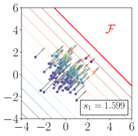
Refer to caption
Refer to caption
Refer to caption
Refer to caption
Refer to caption
Refer to caption
Refer to caption
Refer to caption
Figure 3: Evolution of the iCEred method for problems with (top r=1<d𝑟1𝑑r=1<d) and without (bottom r=2=d𝑟2𝑑r=2=d) intrinsic low-dimensional structure of the parameter space. The arrows show the values of lnf(𝜽;sj)𝑓𝜽subscript𝑠𝑗\nabla\ln f(\bm{\theta};s_{j}) and the color in the samples correspond to the magnitude of the smooth indicator function f(𝜽;sj)𝑓𝜽subscript𝑠𝑗f(\bm{\theta};s_{j}).

4.2 Refinement step

Computational approaches such as adjoint methods [1, 10] and automatic differentiation [24] can be used to calculate efficiently the gradient of the log-smooth indicator function in Eq. 32. However, when these tools are not applicable, gradient evaluation is a computationally demanding task.

This motivates the definition of a refinement step for the iCEred method that allows improving the failure probability estimate, keeping the number of gradient evaluation fixed. The idea is to employ the reference parameters of the low-dimensional biasing density at the last level, to draw additional samples from the fitted parametric density. Such strategy has been applied to the standard CE method in [46]. This complementary step to iCEred adaptively increases the LSF evaluations but it does not involve additional gradient computations. The sample size is augmented at each iteration to obtain new LSF evaluations that will improve the IS estimate. The coefficient of variation of the updated failure probability estimate cv^(p^)^cvsubscript^𝑝\widehat{\mathrm{cv}}\left(\widehat{p}_{\mathcal{F}}\right) is then monitored until it reaches a predefined threshold δ¯¯𝛿\overline{\delta}. Since the value of cv^(p^)^cvsubscript^𝑝\widehat{\mathrm{cv}}\left(\widehat{p}_{\mathcal{F}}\right) at each iteration is typically noisy, we control its mean from a set of previous iteration values. Algorithm 2 details this ‘post-processing’ step.

Input : target coefficient of variation of the failure probability estimate δ¯¯𝛿\overline{\delta}, number of iterations after the coefficient of variation is checked m𝑚m, sample size increment M𝑀M, last iCEred iteration values of: reference parameters 𝝊^rsubscript^𝝊𝑟\widehat{\bm{\upsilon}}_{r}, indicator function 𝒅evalsubscript𝒅eval\bm{d}_{\mathrm{eval}}, IS weights 𝒘𝒘\bm{w}, and bases 𝚽r,𝚽subscript𝚽𝑟subscript𝚽perpendicular-to\mathbf{\Phi}_{r},\mathbf{\Phi}_{\perp}
1
2k=1𝑘1k=1
3
4while True do
5       Compute IS estimator p^1Ni=1Ndeval(i)wisubscript^𝑝1𝑁superscriptsubscript𝑖1𝑁subscript𝑑eval𝑖subscript𝑤𝑖\widehat{p}_{\mathcal{F}}\leftarrow\frac{1}{N}\sum_{i=1}^{N}{d}_{\text{eval}}(i)\cdot w_{i}
6      
7      Estimate the variance of the IS estimator 𝕍^[p^]1N1[1Ni=1Ndeval(i)wi2p^2]^𝕍delimited-[]subscript^𝑝1𝑁1delimited-[]1𝑁superscriptsubscript𝑖1𝑁subscript𝑑eval𝑖superscriptsubscript𝑤𝑖2superscriptsubscript^𝑝2\widehat{\mathds{V}}[\widehat{p}_{\mathcal{F}}]\leftarrow\frac{1}{N-1}\left[\frac{1}{N}\sum_{i=1}^{N}{d}_{\text{eval}}(i)\cdot w_{i}^{2}-\widehat{p}_{\mathcal{F}}^{2}\right]
8      
9      Estimate the coefficient of variation cv^(k)𝕍^[p^]/p^^cv𝑘^𝕍delimited-[]subscript^𝑝subscript^𝑝\widehat{\mathrm{cv}}(k)\leftarrow\sqrt{\widehat{\mathds{V}}[\widehat{p}_{\mathcal{F}}]}/\widehat{p}_{\mathcal{F}}
10      
11      if kmodm=0𝑘mod𝑚0k\leavevmode\nobreak\ \mathrm{mod}\leavevmode\nobreak\ m=0 then
12             Compute the mean of the previous m𝑚m values stored in cv^^cv\widehat{\mathrm{cv}} μcv^absentsubscript𝜇^cv\rightarrow\mu_{\widehat{\mathrm{cv}}}
13            
14            if μcv^δ¯subscript𝜇^cv¯𝛿\mu_{\widehat{\mathrm{cv}}}\leq\overline{\delta} then
15                   Break
16             end if
17            
18       else
19             Generate M𝑀M samples from the biasing density in the local FIS 𝜽~rπbias(r)(;𝝊^r)similar-tosubscript~𝜽𝑟superscriptsubscript𝜋bias𝑟subscript^𝝊𝑟\widetilde{\bm{\theta}}_{r}\sim{\pi}_{\text{bias}}^{(r)}(\cdot;\widehat{\bm{\upsilon}}_{r})
20            
21            Generate M𝑀M samples from the prior density in the local CS 𝜽~πpr()()similar-tosubscript~𝜽perpendicular-tosuperscriptsubscript𝜋prperpendicular-to\widetilde{\bm{\theta}}_{\perp}\sim{\pi}_{\text{pr}}^{(\perp)}(\cdot)
22            
23            Contruct the full set of parameter samples 𝜽𝚽r𝜽~r+𝚽𝜽~𝜽subscript𝚽𝑟subscript~𝜽𝑟subscript𝚽perpendicular-tosubscript~𝜽perpendicular-to\bm{\theta}\leftarrow\mathbf{\Phi}_{r}\widetilde{\bm{\theta}}_{r}+\mathbf{\Phi}_{\perp}\widetilde{\bm{\theta}}_{\perp}
24            
25            Evaluate LSF 𝒈evalg(𝜽)subscript𝒈eval𝑔𝜽\bm{g}_{\text{eval}}\leftarrow g(\bm{\theta}) and indicator function 𝒅extra𝒈eval0=𝟙(𝜽)subscript𝒅extrasubscript𝒈eval0subscript1𝜽\bm{d}_{\text{extra}}\leftarrow\bm{g}_{\text{eval}}\leq 0={\mathds{1}_{\mathcal{F}}\!\left(\bm{\theta}\right)}
26            
27            Compute the weights 𝒘extraexp(lnπpr(r)(𝜽~r)lnπbias(r)(𝜽~r;𝝊^r))subscript𝒘extrasuperscriptsubscript𝜋pr𝑟subscript~𝜽𝑟superscriptsubscript𝜋bias𝑟subscript~𝜽𝑟subscript^𝝊𝑟\bm{w}_{\mathrm{extra}}\leftarrow\exp\left(\ln\pi_{\text{pr}}^{(r)}(\widetilde{\bm{\theta}}_{r})-\ln{\pi}_{\text{bias}}^{(r)}(\widetilde{\bm{\theta}}_{r};\widehat{\bm{\upsilon}}_{r})\right)
28            
29            Append the extra indicator function and weight values 𝒅eval[𝒅eval,𝒅extra]subscript𝒅evalsubscript𝒅evalsubscript𝒅extra\bm{d}_{\text{eval}}\leftarrow[\bm{d}_{\text{eval}},\bm{d}_{\text{extra}}] and 𝒘[𝒘,𝒘extra]𝒘𝒘subscript𝒘extra\bm{w}\leftarrow[\bm{w},\bm{w}_{\mathrm{extra}}]
30            
31            kk+1𝑘𝑘1k\leftarrow k+1 and NN+M𝑁𝑁𝑀N\leftarrow N+M
32       end if
33      
34 end while
Output : p^subscript^𝑝\widehat{p}_{\mathcal{F}}
Algorithm 2 Refinement step for iCEred.

5 Numerical experiments

We test the proposed method on three examples. For the first two experiments, the gradient of the LSF is available analytically and the failure probabilities are independent of the dimension of the input parameter space. This allows us to perform several parameter studies to validate the applicability and accuracy of the iCEred method. In the final example, we consider a structural mechanics application involving spatially variable parameters modeled as random fields. In this case, the LSF gradient is computed using the adjoint method, which is derived in Appendix A for this particular problem.

Moreover, we consider the gradients of the natural logarithm of the smooth indicators Eq. 13

(35) lnflog(𝜽;s)=g(𝜽)s[1+tanh(g(𝜽)s)],lnferf(𝜽;s)=g(𝜽)sϕ(g(𝜽)s)Φ(g(𝜽)s),formulae-sequencesuperscript𝑓log𝜽𝑠𝑔𝜽𝑠delimited-[]1tanh𝑔𝜽𝑠superscript𝑓erf𝜽𝑠𝑔𝜽𝑠italic-ϕ𝑔𝜽𝑠Φ𝑔𝜽𝑠\nabla\ln f^{\mathrm{log}}(\bm{\theta};s)=-\dfrac{\nabla g(\bm{\theta})}{s}\left[1+\text{tanh}\left(\dfrac{g(\bm{\theta})}{s}\right)\right],\qquad\nabla\ln f^{\mathrm{erf}}(\bm{\theta};s)=-\dfrac{\nabla g(\bm{\theta})}{s}\cdot\dfrac{\phi\left(-\dfrac{g(\bm{\theta})}{s}\right)}{\Phi\left(-\dfrac{g(\bm{\theta})}{s}\right)},

for the computation of the estimator 𝐇^^𝐇\widehat{\mathbf{H}} in Eq. 32.

In all experiments, the target coefficient of variation for the iCEred method is set to δ=1.5𝛿1.5\delta=1.5 and the tolerance of the certified approximation is ε=0.01𝜀0.01\varepsilon=0.01. For the refinement step, the target coefficient of variation for the failure probability estimate is δ¯=0.05¯𝛿0.05\overline{\delta}=0.05, and the increment in the sample size is M=50𝑀50M=50. The parametric family of biasing densities is chosen as single Gaussian densities, i.e., Π={πbias(𝜽;𝝊)=𝒩(𝜽;𝝊)|𝝊=[𝝁,𝚺]Υ}Πconditional-setsubscript𝜋bias𝜽𝝊𝒩𝜽𝝊𝝊𝝁𝚺Υ\Pi=\{{\pi}_{\text{bias}}(\bm{\theta};\bm{\upsilon})=\mathcal{N}(\bm{\theta};\bm{\upsilon})\;|\;\allowbreak\bm{\upsilon}=[\bm{\mu},\mathbf{\Sigma}]\in\Upsilon\}.

5.1 Linear LSF in varying dimensions

We consider a LSF expressed as a linear combination of d𝑑d independent standard Gaussian random variables [14]:

(36) g(𝜽)=β1di=1dθiwith gradientg(𝜽)=[1d𝟏d]𝖳,formulae-sequence𝑔𝜽𝛽1𝑑superscriptsubscript𝑖1𝑑subscript𝜃𝑖with gradient𝑔𝜽superscriptdelimited-[]1𝑑subscript1𝑑𝖳g(\bm{\theta})=\beta-\frac{1}{\sqrt{d}}\sum_{i=1}^{d}\theta_{i}\qquad\text{with gradient}\quad\nabla g(\bm{\theta})=\left[-\frac{1}{\sqrt{d}}\cdot\mathbf{1}_{d}\right]^{\mathsf{T}},

where β𝛽\beta is a given maximum threshold, and 𝟏dsubscript1𝑑\mathbf{1}_{d} denotes a d𝑑d-dimensional vector containing ones. The probability of failure is independent of the dimension d𝑑d and it can be computed analytically as p=Φ(β)subscript𝑝Φ𝛽p_{\mathcal{F}}=\Phi(-\beta), with Φ()Φ\Phi(\cdot) denoting the standard Gaussian CDF.

We initially test the two smooth approximations of the log-indicator gradient Eq. 35 used within the iCEred method. In this case, the refinement step of the algorithm is not implemented. This is to evaluate the standalone performance of the method. Ten different values of decreasing target failure probabilities are fixed as p=[1×101,1×102,,1×1010]subscript𝑝1superscript1011superscript1021superscript1010p_{\mathcal{F}}=[1\times 10^{-1},1\times 10^{-2},\ldots,\allowbreak 1\times 10^{-10}], which have an associated list of thresholds β=Φ1(p)[1.282,2.326,,6.361]𝛽superscriptΦ1subscript𝑝1.2822.3266.361\beta=-\Phi^{-1}(p_{\mathcal{F}})\approx[1.282,2.326,\ldots,6.361]. Moreover, for each threshold β𝛽\beta, three different dimensions d{2,358,1000}𝑑23581000d\in\{2,358,\allowbreak 1000\} are employed to define the LSF Eq. 36. These allows us to test the method for low- and high-dimensional settings. A parameter study on the number of samples per level is also performed and we choose this value from N{100,250,500,1000}𝑁1002505001000N\in\{100,250,500,1000\}. In this example, there exists a clear low-dimensional structure of the parameter space and the rank of the projector 𝐏rsubscript𝐏𝑟\mathbf{P}_{r} is r=1𝑟1r=1 for all parameter cases.

Figure 4 shows the coefficient of variation of the failure probability estimates, computed as an average of 100100100 independent iCEred runs. One observes that under the LSF Eq. 36, the performance of the iCEred method is independent of the dimension and magnitude of the failure probability. As the number of samples increases, the smooth approximations yield similar results. However, when the number of samples per level is small, the smooth approximation ferfsuperscript𝑓erff^{\mathrm{erf}} which is based on the standard Gaussian CDF produces larger cv^(p^)^cvsubscript^𝑝\widehat{\mathrm{cv}}\left(\widehat{p}_{\mathcal{F}}\right) values. Note in Eq. 35 that the standard Gaussian CDF is evaluated in the denominator. As the number of iCEred levels increases, the smoothing parameter s0𝑠0s\to 0. For very small values of s𝑠s, Φ(g(𝜽)/s)Φ𝑔𝜽𝑠\Phi(-g(\bm{\theta})/s) takes values close to zero, and hence the value of lnf(𝜽;s)𝑓𝜽𝑠\nabla\ln f(\bm{\theta};s) is not defined. When this occurs, the matrix 𝐇^^𝐇\widehat{\mathbf{H}} cannot be estimated and the basis of the previous level is used. Although this problem is inherent to any approximation of the indicator function, it appears that flogsuperscript𝑓logf^{\mathrm{log}} based on the logistic function is more robust than ferfsuperscript𝑓erff^{\mathrm{erf}}. This is probably because ferfsuperscript𝑓erff^{\mathrm{erf}} involves numerical approximation of the error function. As a result, flogsuperscript𝑓logf^{\mathrm{log}} yields more stable results for sample size N=100𝑁100N=100.

d=2𝑑2d=2                                     d=358𝑑358d=358                                     d=1000𝑑1000d=1000
ferfsuperscript𝑓erff^{\text{erf}} Refer to caption Refer to caption Refer to caption
flogsuperscript𝑓logf^{\text{log}} Refer to caption Refer to caption Refer to caption

Figure 4: Coefficient of variation of the failure probability estimate for example 5.1 using different target probabilities of failure, number of samples, smooth indicators (rows), and increasing dimension (columns).

We now fix the smooth approximation of the indicator function to flogsuperscript𝑓logf^{\mathrm{log}} and the threshold to β=3.5𝛽3.5\beta=3.5 (p2.33×104subscript𝑝2.33superscript104p_{\mathcal{F}}\approx 2.33\times 10^{-4}). In Figure 5, we plot a comparison between the iCEred method (without refinement) with the standard CE and iCE methods for increasing dimension of the parameter space and number of samples per level N{250,1000,2500}𝑁25010002500N\in\{250,1000,2500\}. The CE method is implemented with ρ=0.1𝜌0.1\rho=0.1 (cf., Section 2.3) and the iCE method with δ=1.5𝛿1.5\delta=1.5 (cf., Section 2.4); for both approaches the biasing distribution family consist of single Gaussian densities. We observe that the performance of standard CE and iCE methods deteriorates with increasing dimension of the parameter space, and that augmenting the sample size improves the accuracy in the estimation of the target failure probability. This is related to the solution of the stochastic optimization problem required in both approaches, which amounts to fitting high-dimensional Gaussian densities. The number of samples required to properly perform this step depends on the rank of the covariance matrix of the Gaussian biasing density, and it roughly scales quadratically with the dimension. Although the results can improve if other parametric families of biasing densities are employed (as those proposed in [46, 28]), under the Gaussian parametric family the standard methods are inadequate to perform reliability analysis in high dimensions. The iCEred method estimates consistently the target failure probability for all the dimensions and even at small sample size. Since the rank of the projector is r=1𝑟1r=1, the updating of reference parameters in iCEred amounts to fitting one-dimensional Gaussian densities for all the dimension cases.
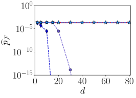
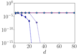
N=250𝑁250N=250                                   N=1000𝑁1000N=1000                                   N=2500𝑁2500N=2500
Refer to caption Refer to caption Refer to caption

Figure 5: Failure probability estimate for example 5.1 using the CE, iCE, and iCEred methods (with single Gaussian parametric family) for increasing dimension of the parameter space and different number of samples per level (columns).

We conclude this example by showing the advantage of the refinement step for iCEred. In this case, the number of samples per level is selected from the set N{100,250,500,1000,2500,5000}𝑁100250500100025005000N\in\{100,250,500,1000,2500,5000\}. Figure 6 shows the number of LSF and gradient calls, together with the coefficient of variation of the failure probability estimate (again, as an average of 100 independent simulations). Note that for sample sizes 100, 250 and 500, there is an increase in the number of LSF evaluations, due to the refinement. This is because small values of N𝑁N are not sufficient to compute a probability of failure estimate that has cv^(p^)^cvsubscript^𝑝\widehat{\mathrm{cv}}\left(\widehat{p}_{\mathcal{F}}\right) smaller than the value of δ¯¯𝛿\overline{\delta}. Therefore, extra LSF computations are performed in the refinement algorithm to reduce the cv^(p^)^cvsubscript^𝑝\widehat{\mathrm{cv}}\left(\widehat{p}_{\mathcal{F}}\right) to δ¯¯𝛿\overline{\delta}. For large sample sizes, this step has no effect since the cv^(p^)^cvsubscript^𝑝\widehat{\mathrm{cv}}\left(\widehat{p}_{\mathcal{F}}\right) obtained from iCEred is already below the predefined δ¯¯𝛿\overline{\delta}.

d=2𝑑2d=2                                       d=358𝑑358d=358                                     d=1000𝑑1000d=1000
Refer to caption Refer to caption Refer to caption

Figure 6: iCEred with refinement for example 5.1: number of LSF and gradient calls for different number of samples, and dimensions (columns). The cv^^cv\widehat{\mathrm{cv}} of the failure probability estimate is also shown (in red).

5.2 Quadratic LSF in varying dimensions

We add a quadratic term to the LSF Eq. 36:

(37a) g(𝜽)𝑔𝜽\displaystyle g(\bm{\theta}) =β+κ4(θ1θ2)21di=1dθiwith gradientabsent𝛽𝜅4superscriptsubscript𝜃1subscript𝜃221𝑑superscriptsubscript𝑖1𝑑subscript𝜃𝑖with gradient\displaystyle=\beta+\frac{\kappa}{4}\left(\theta_{1}-\theta_{2}\right)^{2}-\frac{1}{\sqrt{d}}\sum_{i=1}^{d}\theta_{i}\qquad\text{with gradient}
(37b) g(𝜽)𝑔𝜽\displaystyle\nabla g(\bm{\theta}) =[κ2(θ1θ2)1d,κ2(θ2θ1)1d,1d𝟏d2]𝖳,absentsuperscript𝜅2subscript𝜃1subscript𝜃21𝑑𝜅2subscript𝜃2subscript𝜃11𝑑1𝑑subscript1𝑑2𝖳\displaystyle=\left[\frac{\kappa}{2}(\theta_{1}-\theta_{2})-\frac{1}{\sqrt{d}},\leavevmode\nobreak\ \frac{\kappa}{2}(\theta_{2}-\theta_{1})-\frac{1}{\sqrt{d}},\leavevmode\nobreak\ -\frac{1}{\sqrt{d}}\cdot\mathbf{1}_{d-2}\right]^{\mathsf{T}},

where β=4𝛽4\beta=4 and the parameter κ𝜅\kappa defines the curvature of the LSF at the point in the parameter space with the largest probability density (the larger the curvature, the smaller psubscript𝑝p_{\mathcal{F}}). The reference probability of failure is independent of the dimension and it can be computed as p=ϕ(u+v2(κ/2))ϕ(v)dudvsubscript𝑝superscriptsubscriptsuperscriptsubscriptitalic-ϕ𝑢superscript𝑣2𝜅2italic-ϕ𝑣differential-d𝑢differential-d𝑣p_{\mathcal{F}}=\int_{-\infty}^{\infty}\int_{-\infty}^{\infty}\phi(-u+v^{2}(\kappa/2))\phi(v)\leavevmode\nobreak\ \mathrm{d}u\mathrm{d}v, where ϕitalic-ϕ\phi denotes the standard Gaussian density [27]. We employ the iCEred method with adaptation to estimate the probability of failure associated to the LSF Eq. 37a. The target failure probabilities are p[6.62×106,4.73×106]subscript𝑝6.62superscript1064.73superscript106p_{\mathcal{F}}\approx[6.62\times 10^{-6},4.73\times 10^{-6}] for curvature values κ{5,10}𝜅510\kappa\in\{5,10\}. Three different dimensions d{2,334,1000}𝑑23341000d\in\{2,334,1000\} are employed to define the LSF.
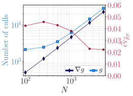
d=2𝑑2d=2                                         d=334𝑑334d=334                                     d=1000𝑑1000d=1000
Refer to caption Refer to caption Refer to caption

Figure 7: Eigenvalue decay (1st row) and first two eigenvectors (2nd row) of the matrix 𝐇^^𝐇\widehat{\mathbf{H}} corresponding to example 5.2 with κ=5𝜅5\kappa=5, for different number of samples and increasing dimension (columns).

d=2𝑑2d=2                                      d=334𝑑334d=334                                   d=1000𝑑1000d=1000
κ=5𝜅5\kappa=5 Refer to caption Refer to caption Refer to caption
κ=10𝜅10\kappa=10 Refer to caption Refer to caption Refer to caption

Figure 8: iCEred with refinement for example 5.2: number of LSF and gradient calls for varying sample size, curvature values (rows) and dimensions (columns). The cv^^cv\widehat{\mathrm{cv}} of the failure probability estimate is also shown (in red).

In Figure 7, we plot the eigenvalue decay and first two eigenvectors of the estimator 𝐇^^𝐇\widehat{\mathbf{H}}, for different number of samples per level N{100,500,1000}𝑁1005001000N\in\{100,500,1000\} and a fixed curvature κ=5𝜅5\kappa=5. The results are for illustration purposes only since they correspond to a single iCEred run. We note that these eigenpairs correspond to the eigendecomposition of 𝐇^^𝐇\widehat{\mathbf{H}} at the last iCEred iteration. The rank of the projector is r=2𝑟2r=2 and it is constant through all the iCEred levels. As in example 5.1, this is a problem with a clear low-dimensional structure since only the parameter components θ1subscript𝜃1\theta_{1} and θ2subscript𝜃2\theta_{2} define the geometry of the LSF; the remaining components represent a linear extrusion in the complementary directions. Thus, the rank remains unchanged even when using small number of samples per level. Note also that for d=2𝑑2d=2 there is no associated dimension reduction and the iCEred method reduces to standard iCE (as seen in Fig. 3).

Figure 8 shows the number of calls of the LSF and its gradient, together with the coefficient of variation of the failure probability estimates; the number of samples per level is now chosen as N{100,250,500,1000,2500,5000}𝑁100250500100025005000N\in\{100,250,500,1000,2500,5000\}. The results are computed as an average of 100 independent runs. Since we perform refinement, all cv^(p^)^cvsubscript^𝑝\widehat{\mathrm{cv}}\left(\widehat{p}_{\mathcal{F}}\right) values are close to the predefined δ¯¯𝛿\overline{\delta} for sample size smaller than N=1000𝑁1000N=1000. This behavior is similar for all studied dimension cases. Although the curvature parameter increases the nonlinearity of the problem, the performance of iCEred remains insensitive to this value. For instance, when using N=1000𝑁1000N=1000 samples per level, the failure probability estimates are p^[6.61×106,4.74×106]subscript^𝑝6.61superscript1064.74superscript106\widehat{p}_{\mathcal{F}}\approx[6.61\times 10^{-6},4.74\times 10^{-6}].

5.3 2D plate in plane stress: LSF with random fields

We consider a steel plate model defined by a square domain D𝐷D with length 0.320.320.32 m, thickness t=0.01𝑡0.01t=0.01 m, and a hole of radius 0.020.020.02 m located at its center. Spatial coordinates are denoted by 𝒙=[x1,x2]D𝒙subscript𝑥1subscript𝑥2𝐷\bm{x}=[x_{1},x_{2}]\in D. The displacement field 𝒖(𝒙):=[ux1(𝒙),ux2(𝒙)]𝖳assign𝒖𝒙superscriptsubscript𝑢subscript𝑥1𝒙subscript𝑢subscript𝑥2𝒙𝖳\bm{u}(\bm{x}):=[u_{x_{1}}(\bm{x}),u_{x_{2}}(\bm{x})]^{\mathsf{T}} is computed using elasticity theory through a set of elliptic PDEs (Cauchy–Navier equations) [19]. Due to the geometry of the plate, the PDEs can be simplified under the plane stress hypothesis to

(38) G(𝒙)2𝒖(𝒙)+E(𝒙)2(1ν)(𝒖(𝒙))+𝐛=0,𝐺𝒙superscript2𝒖𝒙𝐸𝒙21𝜈𝒖𝒙𝐛0G(\bm{x})\nabla^{2}\bm{u}(\bm{x})+\frac{E(\bm{x})}{2(1-\nu)}\nabla(\nabla\cdot\bm{u}(\bm{x}))+\mathbf{b}=0,

where G(𝒙):=E(𝒙)/(2(1+ν))assign𝐺𝒙𝐸𝒙21𝜈G(\bm{x}):=E(\bm{x})/(2(1+\nu)) is the shear modulus, ν=0.29𝜈0.29\nu=0.29 is the Poisson ratio of the steel, and 𝐛𝐛\mathbf{b} is the vector of body forces acting on the plate, assumed to be negligible.

A Dirichlet boundary condition is imposed at the left edge of the plate, 𝒖(𝒙)=𝟎𝒖𝒙0\bm{u}(\bm{x})=\bm{0} for 𝒙Γ1𝒙subscriptΓ1\bm{x}\in\Gamma_{1}. Moreover, a random surface load q𝑞q is applied at the right boundary Γ2subscriptΓ2\Gamma_{2}. This action is modeled as a Gaussian random variable with mean μq=60subscript𝜇𝑞60\mu_{q}=60 MPa and standard deviation σq=12subscript𝜎𝑞12\sigma_{q}=12 MPa. Equation 38 is solved with the finite element method using 282282282 eight-node serendipity quadrilateral elements [26], as shown in Figure 9.
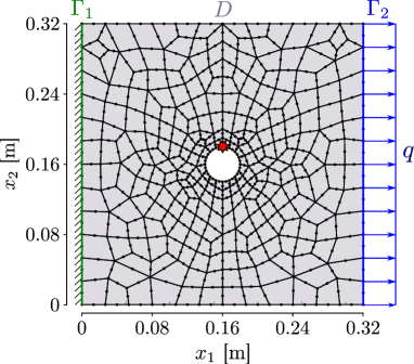
Refer to caption
Figure 9: Plate configuration (star marks the location of the control node).

The Young’s modulus E(𝒙)𝐸𝒙E(\bm{x}) is random and spatially variable. A log-normal random field with mean value μE=2×10⁵subscript𝜇𝐸2superscript105\mu_{E}=2\times 10^{5} MPa and standard deviation σE=3×10⁴subscript𝜎𝐸3superscript104\sigma_{E}=3\times 10^{4} MPa is used for its representation. We select the isotropic exponential kernel k(𝒙,𝒙)=exp(1𝒙𝒙2)𝑘𝒙superscript𝒙superscript1subscriptnorm𝒙superscript𝒙2k(\bm{x},\bm{x}^{\prime})=\exp(-\ell^{-1}\left\|\bm{x}-\bm{x}^{\prime}\right\|_{2}) as the autocorrelation function of the underlying Gaussian field; the correlation length is set to =0.040.04\ell=0.04 m. The random field is approximated with the Karhunen–Loève (K-L) expansion as [17]

(39) E(𝒙)E^(𝒙;𝜽(K-L)):=exp[μE+k=1Kαkφk(𝒙)θk(K-L)],𝐸𝒙^𝐸𝒙superscript𝜽K-Lassignsubscript𝜇superscript𝐸superscriptsubscript𝑘1𝐾subscript𝛼𝑘subscript𝜑𝑘𝒙superscriptsubscript𝜃𝑘K-LE(\bm{x})\approx\widehat{E}\big{(}\bm{x};\bm{\theta}^{(\text{K-L})}\big{)}:=\exp\left[\mu_{E^{\prime}}+\sum_{k=1}^{K}\sqrt{\alpha_{k}}\varphi_{k}(\bm{x})\theta_{k}^{(\text{K-L})}\right],

where μEsubscript𝜇superscript𝐸\mu_{E^{\prime}} and σEsubscript𝜎superscript𝐸\sigma_{E^{\prime}} are the mean and standard deviation of the associated Gaussian field, αk[0,)subscript𝛼𝑘0\alpha_{k}\in[0,\infty) (αkαk+1subscript𝛼𝑘subscript𝛼𝑘1\alpha_{k}\geq\alpha_{k+1} and limkαk=0subscript𝑘subscript𝛼𝑘0\lim_{k\rightarrow\infty}\alpha_{k}=0), φk(𝒙)subscript𝜑𝑘𝒙\varphi_{k}(\bm{x}) are the eigenvalues and eigenfunctions of the covariance operator C(𝒙,𝒙)=σE2k(𝒙,𝒙)𝐶𝒙superscript𝒙superscriptsubscript𝜎superscript𝐸2𝑘𝒙superscript𝒙C(\bm{x},\bm{x}^{\prime})=\sigma_{E^{\prime}}^{2}\cdot k(\bm{x},\bm{x}^{\prime}), and 𝜽(K-L)Ksuperscript𝜽K-Lsuperscript𝐾\bm{\theta}^{(\text{K-L})}\in\mathbbm{R}^{K} is the standard Gaussian random vector of K-L coefficients. The number of terms in the expansion is fixed to K=868𝐾868K=868, which accounts for 92.5%percent92.592.5\% of the spatial average of the variance of the Gaussian random field (lnE𝐸\ln E). The eigenpairs are estimated with the Nyström method using 100100100 Gauss–Legendre (GL) points in each direction.

We select the principal stress σ1(𝝈)=1/2(σx1+σx2)+[(1/2(σx1σx2))2+τx1x22]1/2subscript𝜎1𝝈12subscript𝜎subscript𝑥1subscript𝜎subscript𝑥2superscriptdelimited-[]superscript12subscript𝜎subscript𝑥1subscript𝜎subscript𝑥22superscriptsubscript𝜏subscript𝑥1subscript𝑥2212{\sigma}_{1}(\bm{\sigma})=\nicefrac{{1}}{{2}}\left(\sigma_{x_{1}}+\sigma_{x_{2}}\right)+[\left(\nicefrac{{1}}{{2}}\left(\sigma_{x_{1}}-\sigma_{x_{2}}\right)\right)^{2}+\tau_{x_{1}x_{2}}^{2}]^{\nicefrac{{1}}{{2}}} as the target QoI. This quantity depends on the stress field of the plate 𝝈(𝒙):=[σx1(𝒙),σx2(𝒙),τx1x2(𝒙)]𝖳assign𝝈𝒙superscriptsubscript𝜎subscript𝑥1𝒙subscript𝜎subscript𝑥2𝒙subscript𝜏subscript𝑥1subscript𝑥2𝒙𝖳\bm{\sigma}(\bm{x}):=[\sigma_{x_{1}}(\bm{x}),\sigma_{x_{2}}(\bm{x}),\allowbreak\tau_{x_{1}x_{2}}(\bm{x})]^{\mathsf{T}}, which is computed after obtaining the displacement field via Eq. 38 and applying Hooke’s law for continuous media (see [39] for details). The failure of the plate occurs when the value of σ1subscript𝜎1\sigma_{1} at a control point 𝒙ctr=[0.16,0.18]subscript𝒙ctr0.160.18\bm{x}_{\mathrm{ctr}}=[0.16,0.18] exceeds a yield tensile strength of 320320320 MPa. The LSF is defined as

(40) g(𝜽)=320σ1(𝝈(𝒙ctr;𝜽)).𝑔𝜽320subscript𝜎1𝝈subscript𝒙ctr𝜽g(\bm{\theta})=320-\sigma_{1}(\bm{\sigma}(\bm{x}_{\mathrm{ctr}};\bm{\theta})).

The σ1subscript𝜎1\sigma_{1} stress defining the LSF is evaluated at the GL point of the element closest to the control node 𝒙ctrsubscript𝒙ctr\bm{x}_{\mathrm{ctr}}. The uncertain parameter vector 𝜽=[θ(q),𝜽(K-L)]𝜽superscript𝜃𝑞superscript𝜽K-L\bm{\theta}=[{\theta}^{(q)},\bm{\theta}^{(\text{K-L})}] includes the load random variable and the Young’s modulus random field. The random variable θ(q)superscript𝜃𝑞\theta^{(q)} is also standard Gaussian since we apply the transformation θ(q)=(qμq)/σqsuperscript𝜃𝑞𝑞subscript𝜇𝑞subscript𝜎𝑞\theta^{(q)}=(q-\mu_{q})/\sigma_{q}. The stochastic dimension of the problem is d=K+1=869𝑑𝐾1869d=K+1=869.

This example cannot be solved efficiently using standard CE or iCE, since a large number of effective samples per level are required for fitting high-dimensional parametric densities. Therefore, to compare the results of iCEred, we estimate the failure probability by an average of 100 independent runs of subset simulation (SuS) using N=3000𝑁3000N=3000 samples per level [4]. Although it tends to produce failure probability estimates with a relatively high coefficient of variation, SuS is the standard algorithm for solving efficiently reliability problems in high dimensions.

Table 1: Failure probability estimates: the iCEred results are shown as an average of 40 simulations; the SuS estimate is computed as an average of 100 simulations.
iCEred SuS
N𝑁N gcallsubscript𝑔callg_{\mathrm{call}} (g)callsubscript𝑔call(\nabla g)_{\mathrm{call}} p^subscript^𝑝\widehat{p}_{\mathcal{F}} cv^(p)^cvsubscript𝑝\widehat{\mathrm{cv}}\left(p_{\mathcal{F}}\right) N𝑁N nlvsubscript𝑛lvn_{\mathrm{lv}} gcallsubscript𝑔callg_{\mathrm{call}} p^subscript^𝑝\widehat{p}_{\mathcal{F}} cv^(p)^cvsubscript𝑝\widehat{\mathrm{cv}}\left(p_{\mathcal{F}}\right)
100 2396 675 3.57×1063.57superscript1063.57\times 10^{-6} 0.050 3000 6 1.62×1041.62superscript1041.62\times 10^{4} 3.75×1063.75superscript1063.75\times 10^{-6} 0.215
250 2416 1612 3.60×1063.60superscript1063.60\times 10^{-6} 0.046
500 3685 3037 3.62×1063.62superscript1063.62\times 10^{-6} 0.043

We apply the iCEred method with number of samples per level selected from the set N{100,250,500}𝑁100250500N\in\{100,250,500\}. Table 1 shows the results as an average of 40 independent simulations. Note that the coefficient of variation of the failure probabilities are close to the target δ¯¯𝛿\overline{\delta}. This is also reflected in the averaged number of LSF and gradient calls, denoted respectively as gcallsubscript𝑔callg_{\mathrm{call}} and (g)callsubscript𝑔call(\nabla g)_{\mathrm{call}}. Both number of evaluations are the same when refinement is not required, and the values are closer to each other when number of required iterations in the refinement step is small. As seen also in the previous examples, the value of gcallsubscript𝑔callg_{\mathrm{call}} increases considerably at a small value of N𝑁N in order to match δ¯¯𝛿\overline{\delta}. However, there is a trade-off between the computational cost of the extra LSF and the LSF gradient calls. If the gradient is expensive to evaluate, a small number of samples is recommended since the value of the probability estimate is later improved by the refinement. On the contrary, if an efficient way to compute the LSF gradient is available, the extra LSF evaluations in the refinement might exceed the cost of the gradient computations; in this case using a large sample size is recommended. Note also in Table 1 that the mean value of the probability of failure computed by repeated runs of SuS is close to the values estimated by repeated runs of iCEred, whereas the coefficient of variation of the SuS estimate is significantly higher than the one of iCEred. Moreover, the iCEred method requires considerably fewer LSF evaluations, and thus can be much more efficient than SuS provided an effective gradient computation is feasible.
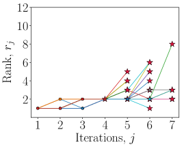
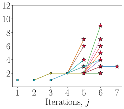
N=100𝑁100N=100                                N=250𝑁250N=250                                 N=500𝑁500N=500
Refer to caption Refer to caption Refer to caption

Figure 10: Example 5.3: evolution of the rank with the iCEred iterations for several simulation runs and N{100,250,500}𝑁100250500N\in\{100,250,500\} (columns). The star marks the final value of the rank at the given simulation run.

We plot in Figure 10 the evolution of the rank with the iCEred iterations (intermediate levels). The results are shown for different sample sizes and independent simulation runs. As N𝑁N increases the number of iterations becomes smaller; on average, for each of the employed sample sizes, the number of levels are nlv=[5.75,5.45,5.08]subscript𝑛lv5.755.455.08n_{\mathrm{lv}}=[5.75,5.45,5.08]. For the investigated number of samples per level, the maximum observed ranks across the 40 independent simulations are r=[8,9,12]𝑟8912r=[8,9,12]; however, the final rank is on average r=3𝑟3r=3 for N=100𝑁100N=100, and r=4𝑟4r=4 for N=[250,500]𝑁250500N=[250,500]. We also observe that the value of the smoothing parameters at the final iteration are on average snlv=[0.098,0.084,0.051]subscript𝑠subscript𝑛lv0.0980.0840.051s_{n_{\mathrm{lv}}}=[0.098,0.084,0.051], which shows that s𝑠s reaches values closer to zero for larger sample sizes. Note in Eq. 35 that the gradient of the log-smooth indicator is essentially driven by the gradient of the LSF; the smoothing parameter indirectly determines the locations at which the gradient is evaluated. In this example, the increment in the rank with the number of intermediate levels seems to be related to the LSF gradient discovering a larger FIS as the samples move towards the failure domain where the nonlinearity of the LSF increases.
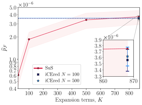
Refer to caption
Figure 11: Example 5.3: probability of failure estimated by SuS at selected truncation orders in the K-L expansion (mean and standard deviation bounds), and probability of failure estimated by iCEred at the K=868𝐾868K=868 term (zoomed area: mean and standard deviation bounds).

Finally, Figure 11 shows the evolution of the probability of failure for increasing terms in the K-L expansion Eq. 39. Different failure probabilities are computed by SuS for truncation orders K{25,100,500,868}𝐾25100500868K\in\{25,100,500,\allowbreak 868\}; the iCEred method is only evaluated for K=868𝐾868K=868. In both approaches, the estimators are given as average of 40 independent simulations. Note the difference between the failure probabilities computed by reducing the number of input dimensions (K-L terms) and those estimated by identifying the FIS. Solving the rare event simulation problem on the FIS is not equivalent to truncating the parameter space, as in the latter case, there is an associated loss of information (e.g., random field variability). The effective dimension of the local FIS in this example is on average r=4𝑟4r=4 (when using N=500𝑁500N=500 samples), and thus the iCEred method can compute the failure probability associated with an input dimension of K=868𝐾868K=868 efficiently and with a very small coefficient of variation.

6 Summary and conclusions

We developed a computational framework for solving high-dimensional rare event simulation problems. This includes settings where the underlying system properties are spatially inhomogeneous and random field models are required for their representation. The approach (called iCEred) is an extension of importance sampling with the cross-entropy method that enhances its efficiency in high dimensions. The main idea is to adapt dimension reduction techniques developed for Bayesian inference through expressing rare event simulation as a Bayesian inversion problem. This enables the identification of the potential low-dimensional structure of the rare event simulation problem. As a result, we construct a so-called failure-informed subspace, where efficient low-dimensional biasing distributions for importance sampling can be defined. This process ultimately requires the computation of the limit-state function gradient.

When the limit-state function is highly nonlinear, the rank of the projectors that map the parameters onto the failure-informed subspace increases as one approaches the final iterations of the algorithm. This indicates that when the smooth approximation gravitates to the indicator function, the gradient samples are discovering a larger subspace due to the increase in nonlinearity at the failure region.

The numerical experiments show that the iCEred is able to effectively compute rare event probability estimates in high dimensions with considerably smaller variability and required sample size compared to standard simulation approaches that typically rely on Markov chain Monte Carlo. We also remark that when dealing with problems that have multiple failure points (multi-modal failure hypersurface), mixture distributions can also be adapted within the iCEred framework.

A possible improvement of the method is to define a measure to assess whether or not the second moment matrix of the gradient of the log-smooth indicator function needs to be computed at a given level. Since the main interest is the estimation of the failure probability and not the construction of the optimal biasing distribution itself, it might be sufficient to build the failure-informed space at the initial iterations and continue with the standard methodology in the remainder levels. Furthermore, rather than using the same sample size for the limit-state function evaluations and gradient computations, one can define two different sample sizes. The number of samples per level required to evaluate the gradient can be adapted based on the value of the rank at the given intermediate level. These suggestions could potentially save significant computational demands related to gradient evaluations in iCEred. Moreover, the low-dimensional structure of the failure-informed subspace can be exploited in other rare event simulation algorithms.

Appendix A Adjoint solution

In example 5.3, the eigenfunctions of the covariance operator are interpolated at the GL points of the finite element mesh using Nyström formula [31]. Thus, for a nGPsubscript𝑛GPn_{\mathrm{GP}}-point spatial discretization, the K-L representation of the Young’s modulus truncated at the K𝐾K-th term is expressed in matrix form as 𝑬^=exp[μE+𝐀𝜽(KL)]^𝑬subscript𝜇superscript𝐸𝐀superscript𝜽KL\widehat{\bm{E}}=\exp\left[\mu_{E^{\prime}}+\mathbf{A}\bm{\theta}^{(\mathrm{K-L})}\right], where 𝚽𝚲=𝐀nGP×K𝚽𝚲𝐀superscriptsubscript𝑛GP𝐾\bm{\Phi}\bm{\Lambda}=\mathbf{A}\in\mathbbm{R}^{n_{\mathrm{GP}}\times K}, 𝚲=diag(𝝀)K×K𝚲diag𝝀superscript𝐾𝐾\bm{\Lambda}=\text{diag}(\sqrt{\bm{\lambda}})\in\mathbbm{R}^{K\times K} is a diagonal matrix with the square root of the eigenvalues of the covariance operator, and 𝚽nGP×K𝚽superscriptsubscript𝑛GP𝐾\bm{\Phi}\in\mathbbm{R}^{n_{\mathrm{GP}}\times K} is a matrix containing the associated eigenfunctions evaluated at the GL points.

For a given realization of the uncertain parameters 𝜽=[θ(q),𝜽(K-L)]𝜽superscript𝜃𝑞superscript𝜽K-L\bm{\theta}=[{\theta}^{(q)},\bm{\theta}^{(\text{K-L})}], the finite element formulation yields the global matrix equilibrium equation 𝐊(𝜽)𝒖(𝜽)=𝒇(𝜽)𝐊𝜽𝒖𝜽𝒇𝜽\mathbf{K}(\bm{\theta})\bm{u}(\bm{\theta})=\bm{f}(\bm{\theta}), where 𝐊ndof×ndof𝐊superscriptsubscript𝑛dofsubscript𝑛dof\mathbf{K}\in\mathbbm{R}^{n_{\text{dof}}\times n_{\text{dof}}} is the stiffness matrix, 𝒇ndof𝒇superscriptsubscript𝑛dof\bm{f}\in\mathbbm{R}^{n_{\text{dof}}} is the force vector, and 𝒖ndof𝒖superscriptsubscript𝑛dof\bm{u}\in\mathbbm{R}^{n_{\text{dof}}} is the vector of displacements; ndofsubscript𝑛dofn_{\text{dof}} denotes the total number of degrees of freedom. Furthermore, the stress field can be computed at a specific GL point as,

(41) 𝝈(𝜽)=(𝐃(𝜽)𝐁𝐌)𝒖(𝜽)superscript𝝈𝜽superscript𝐃𝜽superscript𝐁𝐌𝒖𝜽\bm{\sigma}^{\star}(\bm{\theta})=\left(\mathbf{D}^{\star}(\bm{\theta})\leavevmode\nobreak\ \mathbf{B}^{\star}\leavevmode\nobreak\ \mathbf{M}\right)\bm{u}(\bm{\theta})

where the constitutive matrix 𝐃3×3superscript𝐃superscript33\mathbf{D}^{\star}\in\mathbbm{R}^{3\times 3} and the deformation matrix 𝐁3×neqsuperscript𝐁superscript3subscript𝑛eq\mathbf{B}^{\star}\in\mathbbm{R}^{3\times n_{\text{eq}}} are those evaluated at the GL point closest to the control point (cf., Figure 9). In our case, the number of element equations is neq=16subscript𝑛eq16n_{\text{eq}}=16, since there are two degrees of freedom for each element node. Note that in Eq. 41, we employ a matrix 𝐌neq×ndof𝐌superscriptsubscript𝑛eqsubscript𝑛dof\mathbf{M}\in\mathbbm{R}^{n_{\text{eq}}\times n_{\text{dof}}} to ‘activate’ the degrees of freedom corresponding to the nodes of the element that has the control point as one of its nodes.

Our aim is to compute directly the gradient of the principal stress σ1(𝝈(𝐃(𝜽),𝒖(𝜽)))subscript𝜎1superscript𝝈𝐃𝜽𝒖𝜽{\sigma}_{1}(\bm{\sigma}^{\star}(\mathbf{D}(\bm{\theta}),\bm{u}(\bm{\theta}))) with respect to 𝜽𝜽\bm{\theta}. We consider the total derivative

(42) dσ1d𝜽=dσ1d𝝈(d𝝈d𝐃d𝐃d𝜽+d𝝈d𝒖d𝒖d𝜽).dsubscript𝜎1d𝜽dsubscript𝜎1dsuperscript𝝈dsuperscript𝝈dsuperscript𝐃dsuperscript𝐃d𝜽dsuperscript𝝈d𝒖d𝒖d𝜽\frac{\mathrm{d}{\sigma}_{1}}{\mathrm{d}\bm{\theta}}=\frac{\mathrm{d}{\sigma}_{1}}{\mathrm{d}\bm{\sigma}^{\star}}\Big{(}\frac{\mathrm{d}\bm{\sigma}^{\star}}{\mathrm{d}\mathbf{D}^{\star}}\frac{\mathrm{d}\mathbf{D}^{\star}}{\mathrm{d}\bm{\theta}}+\frac{\mathrm{d}\bm{\sigma}^{\star}}{\mathrm{d}\bm{u}}\frac{\mathrm{d}\bm{u}}{\mathrm{d}\bm{\theta}}\Big{)}.

The multiplicative term in Eq. 42 is obtained from the definition of the σ1subscript𝜎1\sigma_{1} stress

(43) dσ1d𝝈=[12(1+σxσy2e),12(1σxσy2e),τxye],e=(σxσy2)2+τxy2.formulae-sequencedsubscript𝜎1dsuperscript𝝈121subscriptsuperscript𝜎𝑥subscriptsuperscript𝜎𝑦2𝑒121subscriptsuperscript𝜎𝑥subscriptsuperscript𝜎𝑦2𝑒subscriptsuperscript𝜏𝑥𝑦𝑒𝑒superscriptsubscriptsuperscript𝜎𝑥subscriptsuperscript𝜎𝑦22superscriptsubscriptsuperscript𝜏𝑥𝑦2\frac{\mathrm{d}{\sigma}_{1}}{\mathrm{d}\bm{\sigma}^{\star}}=\left[\frac{1}{2}\left(1+\frac{{\sigma}^{\star}_{x}-{\sigma}^{\star}_{y}}{2e}\right),\frac{1}{2}\left(1-\frac{{\sigma}^{\star}_{x}-{\sigma}^{\star}_{y}}{2e}\right),\frac{{\tau}^{\star}_{xy}}{e}\right],\quad e=\sqrt{{\left(\frac{{\sigma}^{\star}_{x}-{\sigma}^{\star}_{y}}{2}\right)}^{2}+{{\tau}^{\star}_{xy}}^{2}}.

To compute the first term inside the parenthesis Eq. 42, we use the fact that the element constitutive matrix can be factored as 𝑬^𝐃0=𝐃^𝑬subscript𝐃0𝐃\widehat{\bm{E}}\cdot\mathbf{D}_{0}=\mathbf{D} (under plane stress assumption [26, p.122]), and that the derivative of the K-L expansion of a lognormal field is 𝑬^𝐀=𝑬^nGP×K^𝑬𝐀superscript^𝑬superscriptsubscript𝑛GP𝐾\widehat{\bm{E}}\mathbf{A}=\widehat{\bm{E}}^{\prime}\in\mathbbm{R}^{n_{\mathrm{GP}}\times K}. Hence,

(44) d𝝈d𝐃=(𝐁𝐌)𝒖andd𝐃d𝜽=d𝐃d𝑬^d𝑬^d𝜽(KL)=𝐃0𝑬^,formulae-sequencedsuperscript𝝈dsuperscript𝐃superscript𝐁𝐌𝒖anddsuperscript𝐃d𝜽dsuperscript𝐃d^𝑬d^𝑬dsuperscript𝜽KLsubscript𝐃0superscript^𝑬\frac{\mathrm{d}\bm{\sigma}^{\star}}{\mathrm{d}\mathbf{D}^{\star}}=(\mathbf{B}^{\star}\mathbf{M})\bm{u}\qquad\text{and}\qquad\frac{\mathrm{d}\mathbf{D}^{\star}}{\mathrm{d}\bm{\theta}}=\frac{\mathrm{d}\mathbf{D}^{\star}}{\mathrm{d}\widehat{\bm{E}}}\frac{\mathrm{d}\widehat{\bm{E}}}{\mathrm{d}\bm{\theta}^{(\mathrm{K-L})}}=\mathbf{D}_{0}\widehat{\bm{E}}^{\prime\star},

where 𝑬^Ksuperscript^𝑬superscript𝐾\widehat{\bm{E}}^{\prime\star}\in\mathbbm{R}^{K} is the K-L expansion derivative at the GL point closest to the control node. Moreover, the second term inside the parenthesis in Eq. 42 is

(45) d𝝈d𝒖=𝐃𝐁𝐌andd𝒖d𝜽=𝐊1(d𝒇dθ(q)d𝐊d𝜽(KL)𝒖),formulae-sequencedsuperscript𝝈d𝒖superscript𝐃superscript𝐁𝐌andd𝒖d𝜽superscript𝐊1d𝒇dsuperscript𝜃𝑞d𝐊dsuperscript𝜽KL𝒖\frac{\mathrm{d}\bm{\sigma}^{\star}}{\mathrm{d}\bm{u}}=\mathbf{D}^{\star}\mathbf{B}^{\star}\mathbf{M}\qquad\text{and}\qquad\frac{\mathrm{d}\bm{u}}{\mathrm{d}\bm{\theta}}=\mathbf{K}^{-1}\left(\dfrac{\mathrm{d}\bm{f}}{\mathrm{d}{\theta}^{(q)}}-\dfrac{\mathrm{d}\mathbf{K}}{\mathrm{d}\bm{\theta}^{(\mathrm{K-L})}}\bm{u}\right),

and the components of the derivative d𝒖d𝜽d𝒖d𝜽\frac{\mathrm{d}\bm{u}}{\mathrm{d}\bm{\theta}} are obtained from the finite element formulation as

d𝒇θ(q)=d𝒇dqdqdθ(q)=𝒄σqandd𝐊d𝜽(KL)=eA(e)𝐁(e),𝖳(𝐃0𝑬^(e))𝐁(e)tdA(e),formulae-sequenced𝒇superscript𝜃𝑞d𝒇d𝑞d𝑞dsuperscript𝜃𝑞𝒄subscript𝜎𝑞andd𝐊dsuperscript𝜽KLsubscript𝑒subscriptsuperscript𝐴𝑒superscript𝐁𝑒𝖳subscript𝐃0superscript^𝑬𝑒superscript𝐁𝑒𝑡differential-dsuperscript𝐴𝑒\dfrac{\mathrm{d}\bm{f}}{{\theta}^{(q)}}=\dfrac{\mathrm{d}\bm{f}}{\mathrm{d}{q}}\dfrac{\mathrm{d}{q}}{\mathrm{d}\theta^{(q)}}=\bm{c}\cdot\sigma_{q}\qquad\text{and}\qquad\dfrac{\mathrm{d}\mathbf{K}}{\mathrm{d}\bm{\theta}^{(\mathrm{K-L})}}=\bigcup_{e}\int_{A^{(e)}}\mathbf{B}^{(e),\mathsf{T}}\left(\mathbf{D}_{0}\widehat{\bm{E}}^{\prime(e)}\right)\mathbf{B}^{(e)}\leavevmode\nobreak\ t\leavevmode\nobreak\ \mathrm{d}A^{(e)},

where 𝒄ndof𝒄superscriptsubscript𝑛dof\bm{c}\in\mathbbm{R}^{n_{\mathrm{dof}}} is a constant vector that maps the surface load q𝑞q to equivalent nodal forces, esubscript𝑒\bigcup_{e} denotes assembly procedure over all elements, t𝑡t is the thickness of the plate, and the integration is performed over the area of each element A(e)superscript𝐴𝑒A^{(e)}. The term d𝐊d𝜽(KL)d𝐊dsuperscript𝜽KL\frac{\mathrm{d}\mathbf{K}}{\mathrm{d}\bm{\theta}^{(\mathrm{K-L})}} is a rank-3 tensor with size K×ndof×ndof𝐾subscript𝑛dofsubscript𝑛dofK\times n_{\mathrm{dof}}\times n_{\mathrm{dof}}, and its assembly is in general computationally intensive.

The idea of the adjoint method [1] is to expand and re-organize the terms in Eq. 42 to avoid the computation of expensive matrix operations. Specifically consider the term

(46) dσ1d𝝈d𝝈d𝒖d𝒖d𝜽=dσ1d𝝈d𝝈d𝒖(𝐊1(d𝒇dθ(q)d𝐊d𝜽(KL)𝒖))=dσ1d𝝈d𝝈d𝒖𝐊1𝝀(d𝒇dθ(q)d𝐊d𝜽(KL)𝒖)d𝒑d𝜽,dsubscript𝜎1dsuperscript𝝈dsuperscript𝝈d𝒖d𝒖d𝜽dsubscript𝜎1dsuperscript𝝈dsuperscript𝝈d𝒖superscript𝐊1d𝒇dsuperscript𝜃𝑞d𝐊dsuperscript𝜽KL𝒖subscriptdsubscript𝜎1dsuperscript𝝈dsuperscript𝝈d𝒖superscript𝐊1𝝀subscriptd𝒇dsuperscript𝜃𝑞d𝐊dsuperscript𝜽KL𝒖d𝒑d𝜽\frac{\mathrm{d}{\sigma}_{1}}{\mathrm{d}\bm{\sigma}^{\star}}\frac{\mathrm{d}\bm{\sigma}^{\star}}{\mathrm{d}\bm{u}}\frac{\mathrm{d}\bm{u}}{\mathrm{d}\bm{\theta}}=\frac{\mathrm{d}{\sigma}_{1}}{\mathrm{d}\bm{\sigma}^{\star}}\frac{\mathrm{d}\bm{\sigma}^{\star}}{\mathrm{d}\bm{u}}\left(\mathbf{K}^{-1}\left(\dfrac{\mathrm{d}\bm{f}}{\mathrm{d}{\theta}^{(q)}}-\dfrac{\mathrm{d}\mathbf{K}}{\mathrm{d}\bm{\theta}^{(\mathrm{K-L})}}\bm{u}\right)\right)=\underbrace{\frac{\mathrm{d}{\sigma}_{1}}{\mathrm{d}\bm{\sigma}^{\star}}\frac{\mathrm{d}\bm{\sigma}^{\star}}{\mathrm{d}\bm{u}}\mathbf{K}^{-1}}_{\bm{\lambda}}\underbrace{\left(\dfrac{\mathrm{d}\bm{f}}{\mathrm{d}{\theta}^{(q)}}-\dfrac{\mathrm{d}\mathbf{K}}{\mathrm{d}\bm{\theta}^{(\mathrm{K-L})}}\bm{u}\right)}_{\frac{\mathrm{d}\bm{p}}{\mathrm{d}\bm{\theta}}},

where 𝒑=𝐊𝒖𝒇𝒑𝐊𝒖𝒇\bm{p}=\mathbf{K}\bm{u}-\bm{f}, and the adjoint multiplier 𝝀ndof𝝀superscriptsubscript𝑛dof\bm{\lambda}\in\mathbbm{R}^{n_{\mathrm{dof}}} is computed by solving the adjoint equation

(47) 𝐊𝖳𝝀=[dσ1d𝝈d𝝈d𝒖]𝖳,superscript𝐊𝖳𝝀superscriptdelimited-[]dsubscript𝜎1dsuperscript𝝈dsuperscript𝝈d𝒖𝖳\mathbf{K}^{\mathsf{T}}\bm{\lambda}=\left[\frac{\mathrm{d}{\sigma}_{1}}{\mathrm{d}\bm{\sigma}^{\star}}\frac{\mathrm{d}\bm{\sigma}^{\star}}{\mathrm{d}\bm{u}}\right]^{\mathsf{T}},

we remark that the boundary conditions defining the finite element problem also need to be imposed on Eq. 47. Therefore, finding the gradient dσ1d𝜽=[dσ1dθ(q),dσ1d𝜽(KL)]dsubscript𝜎1d𝜽dsubscript𝜎1dsuperscript𝜃𝑞dsubscript𝜎1dsuperscript𝜽KL\frac{\mathrm{d}{\sigma}_{1}}{\mathrm{d}\bm{\theta}}=\left[\frac{\mathrm{d}{\sigma}_{1}}{\mathrm{d}{\theta}^{(q)}},\frac{\mathrm{d}{\sigma}_{1}}{\mathrm{d}\bm{\theta}^{(\mathrm{K-L})}}\right] amounts to compute

(48) dσ1dθ(q)=𝝀𝖳d𝒇dθ(q)anddσ1d𝜽(KL)=dσ1d𝝈d𝝈d𝐃d𝐃d𝜽+𝝀𝖳(d𝐊d𝜽(KL)𝒖).formulae-sequencedsubscript𝜎1dsuperscript𝜃𝑞superscript𝝀𝖳d𝒇dsuperscript𝜃𝑞anddsubscript𝜎1dsuperscript𝜽KLdsubscript𝜎1dsuperscript𝝈dsuperscript𝝈dsuperscript𝐃dsuperscript𝐃d𝜽superscript𝝀𝖳d𝐊dsuperscript𝜽KL𝒖\frac{\mathrm{d}{\sigma}_{1}}{\mathrm{d}{\theta}^{(q)}}=\bm{\lambda}^{\mathsf{T}}\dfrac{\mathrm{d}\bm{f}}{\mathrm{d}{\theta}^{(q)}}\qquad\text{and}\qquad\frac{\mathrm{d}{\sigma}_{1}}{\mathrm{d}\bm{\theta}^{(\mathrm{K-L})}}=\frac{\mathrm{d}{\sigma}_{1}}{\mathrm{d}\bm{\sigma}^{\star}}\frac{\mathrm{d}\bm{\sigma}^{\star}}{\mathrm{d}\mathbf{D}^{\star}}\frac{\mathrm{d}\mathbf{D}^{\star}}{\mathrm{d}\bm{\theta}}+\bm{\lambda}^{\mathsf{T}}\left(-\dfrac{\mathrm{d}\mathbf{K}}{\mathrm{d}\bm{\theta}^{(\mathrm{K-L})}}\bm{u}\right).

References

  • [1] J. S. Arora and E. J. Haug, Methods of design sensitivity analysis in structural optimization, AIAA Journal, 17 (1979), pp. 970–974.
  • [2] R. B. Ash and C. Doléans-Dade, Probability and measure theory, Harcourt/Academic Press, 2 ed., 2000.
  • [3] S. Asmussen, Large deviations in rare events simulation: examples, counterexamples and alternatives, in Monte Carlo and Quasi-Monte Carlo Methods 2000, K.-T. Fang, H. Niederreiter, and F. J. Hickernell, eds., Springer, 2002, pp. 1–9.
  • [4] S.-K. Au and J. L. Beck, Estimation of small failure probabilities in high dimensions by subset simulation, Probabilistic Engineering Mechanics, 16 (2001), pp. 263–277.
  • [5] Z. I. Botev and D. P. Kroese, Efficient Monte Carlo simulation via the generalized splitting method, Statistics and Computing, 22 (2012), pp. 1–16.
  • [6] Z. I. Botev, D. P. Kroese, and T. Taimre, Generalized cross-entropy methods with applications to rare-event simulation and optimization, SIMULATION, 83 (2007), pp. 785–806.
  • [7] J. A. Bucklew, An introduction to rare event simulation, Springer, 2004.
  • [8] F. Cérou, P. Del Moral, T. Furon, and A. Guyader, Sequential Monte Carlo for rare event estimation, Statistics and Computing, 22 (2012), pp. 795–808.
  • [9] P. G. Constantine, Active subspaces: emerging ideas for dimension reduction in parameter studies, Society for Industrial and Applied Mathematics (SIAM), 2015.
  • [10] P. G. Constantine, E. Dow, and Q. Wang, Active subspace methods in theory and practice: applications to kringing surfaces, SIAM Journal on Scientific Computing, 36 (2014), pp. A1500–A1524.
  • [11] T. Cui, J. Martin, Y. M. Marzouk, A. Solonen, and A. Spantini, Likelihood-informed dimension reduction for nonlinear inverse problems, Inverse Problems, 30 (2014), p. 0114015.
  • [12] P. Del Moral, A. Doucet, and A. Jasra, Sequential Monte Carlo samplers, Journal of the Royal Statistical Society: Series B, 68 (2006), pp. 411–436.
  • [13] O. Ditlevsen, R. E. Melchers, and H. Gluver, General multi-dimensional probability integration by directional simulation, Computers & Structures, 36 (1990), pp. 355–368.
  • [14] S. Engelund and R. Rackwitz, A benchmark study on importance sampling techniques in structural reliability, Structural Safety, 12 (1993), pp. 255–276.
  • [15] B. Fiessler, H.-J. Neumann, and R. Rackwitz, Quadratic limit states in structural reliability, Journal of the Engineering Mechanics Division (ASCE), 105 (1979), pp. 661–676.
  • [16] S. Geyer, I. Papaioannou, and D. Straub, Cross entropy-based importance sampling using Gaussian densities revisited, Structural Safety, 76 (2019), pp. 15–27.
  • [17] R. G. Ghanem and P. D. Spanos, Stochastic finite elements: a spectral approach, Dover Publications, Revised ed., 2012.
  • [18] M. Hohenbichler and R. Rackwitz, Improvement of second-order reliability estimates by importance sampling, Journal of Engineering Mechanics, 114 (1988), pp. 2195–2199.
  • [19] C. Johnson, Numerical solution of partial differential equations by the finite element method, Dover Publications, 2009.
  • [20] H. Kahn and A. W. Marshall, Methods of reducing sample size in Monte Carlo computations, Journal of the Operations Research Society of America, 1 (1953), pp. 263–278.
  • [21] P. S. Koutsourelakis, H. J. Pradlwarter, and G. I. Schuëller, Reliability of structures in high dimensions, part I: algorithms and applications, Probabilistic Engineering Mechanics, 19 (2004), pp. 409–417.
  • [22] S. Lacaze, L. Brevault, S. Missoum, and M. Balesdent, Probability of failure sensitivity with respect to decision variables, Structural and Multidisciplinary Optimization, 52 (2015), pp. 375–381.
  • [23] M. Lemaire, A. Chateauneuf, and J. Mitteau, Structural reliability, Wiley-ISTE, 2009.
  • [24] C. C. Margossian, A review of Automatic Differentiation and its efficient implementation, arXiv:1811.05031v2 eprint, (2019), pp. 1--32.
  • [25] A. B. Owen, Monte Carlo theory, methods and examples, statweb.stanford.edu/similar-to\simowen/mc/, 2013.
  • [26] E. Oñate, Structural analysis with the finite element method. Linear statics. Volume 1: Basis and Solids, Springer, 2009.
  • [27] I. Papaioannou, W. Betz, K. Zwirglmaier, and D. Straub, MCMC algorithms for subset simulation, Probabilistic Engineering Mechanics, 41 (2015), pp. 89--103.
  • [28] I. Papaioannou, S. Geyer, and D. Straub, Improved cross entropy-based importance sampling with a flexible mixture model, Reliability Engineering & System Safety, 191 (2019), p. 106564.
  • [29] I. Papaioannou, C. Papadimitriou, and D. Straub, Sequential importance sampling for structural reliability analysis, Structural Safety, 62 (2016), pp. 66--75.
  • [30] B. Peherstorfer, B. Kramer, and K. Willcox, Multifidelity preconditioning of the cross-entropy method for rare event simulation and failure probability estimation, SIAM/ASA Journal on Uncertainty Quantification, 6 (2018), pp. 737--761.
  • [31] W. H. Press, S. A. Teukolsky, W. T. Vetterling, and B. P. Flannery, Numerical recipes in C: the art of scientific computing, Cambridge University Press, 3 ed., 2007.
  • [32] R. Rackwitz and B. Fiessler, Structural reliability under combined random load sequences, Computers & Structures, 9 (1978), pp. 489--494.
  • [33] J. S. Rosenthal, A first look at rigorous probability theory, World Scientific Publishing Company, 2 ed., 2006.
  • [34] R. Y. Rubinstein, Optimization of computer simulation models with rare events, European Journal of Operational Research, 99 (1997), pp. 89--112.
  • [35] R. Y. Rubinstein and P. W. Glynn, How to deal with the curse of dimensionality of likelihood ratios in Monte Carlo simulation, Stochastic Models, 25 (2009), pp. 547--568.
  • [36] R. Y. Rubinstein and D. P. Kroese, Simulation and the Monte Carlo method, John Wiley & Sons, 3 ed., 2017.
  • [37] R. L. Schilling, Measures, integrals and martingales, Cambridge University Press, 2005.
  • [38] M. Shinozuka, Basic analysis of structural safety, Journal of Structural Engineering, 109 (1983), pp. 721--740.
  • [39] R. Solecki and R. J. Conant, Advanced mechanics of materials, Oxford University Press, 2003.
  • [40] A. Spantini, A. Solonen, T. Cui, J. Martin, L. Tenorio, and Y. Marzouk, Optimal low-rank approximations of Bayesian linear inverse problems, SIAM Journal of Scientific Computing, 37 (2015), pp. A2451--A2487.
  • [41] A. M. Stuart, Inverse problems: a Bayesian perspective, Acta Numerica, 19 (2010), pp. 451--559.
  • [42] E. Ullmann and I. Papaioannou, Multilevel estimation of rare events, SIAM/ASA Journal on Uncertainty Quantification, 3 (2015), pp. 922--953.
  • [43] M. A. Valdebenito, H. J. Pradlwarter, and G. I. Schuëller, The role of the design point for calculating failure probabilities in view of dimensionality and structural nonlinearities, Structural Safety, 32 (2010), pp. 101--111.
  • [44] S. Wahal and G. Biros, BIMC: the Bayesian inverse Monte Carlo method for goal-oriented uncertainty quantification. Part I., arXiv:1911.00619 eprint, (2019), pp. 1--38.
  • [45] S. Wahal and G. Biros, BIMC: the Bayesian inverse Monte Carlo method for goal-oriented uncertainty quantification. Part II., arXiv:1911.01268 eprint, (2019), pp. 1--35.
  • [46] Z. Wang and J. Song, Cross-entropy-based adaptive importance sampling using von Mises-Fisher mixture for high dimensional reliability analysis, Structural Safety, 59 (2016), pp. 42--52.
  • [47] O. Zahm, T. Cui, K. Law, A. Spantini, and Y. Marzouk, Certified dimension reduction in nonlinear Bayesian inverse problems, arXiv:1807.03712v2 eprint, (2018), pp. 1--41.