Fragile extended phases in logarithmically-normal Rosenzweig-Porter model.

Abstract

In this paper we suggest an extension of the Rosenzweig-Porter (RP) model, the LN-RP model, in which the off-diagonal matrix elements have a wide, log-normal distribution. We argue that this model is more suitable to describe a generic many body localization problem. In contrast to RP model, in LN-RP model a fragile weakly ergodic phase appears that is characterized by broken basis-rotation symmetry which the fully-ergodic phase, also present in this model, strictly respects in the thermodynamic limit. Therefore, in addition to the localization and ergodic transitions in LN-RP model there exists also the transition between the two ergodic phases (FWE transition). We suggest new criteria of stability of the non-ergodic phases which give the points of localization and ergodic transitions and prove that the Anderson localization transition in LN-RP model involves a jump in the fractal dimension of the egenfunction support set. We also formulate the criterion of FWE transition and obtain the full phase diagram of the model. We show that truncation of the log-normal tail shrinks the region of weakly-ergodic phase and restores the multifractal and the fully-ergodic phases.

I Introduction

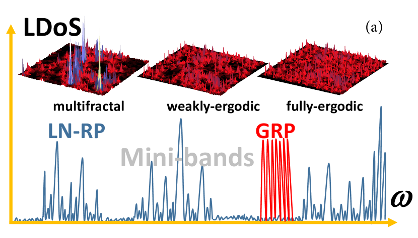
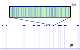
The structure of many body wave function is important for a variety of problems that range from many body localization (MBL) (see Ref. Basko et al. (2006) and a recent review D.A.Abanin et al. (2019)) to quantum computation. It was recently realized that in many of these problems the wave function is neither localized nor completely ergodic Macé et al. (2019); Tarzia (2020); Giuseppe De Tomasi (2020). Instead it is characterized by anomalous dimension, $D_{1}<1$: $\sum_{i}\psi_{\mu}(i)^{2}\ln\psi_{\mu}(i)^{2}=-D_{1}\ln\mathcal{N}$, where $\mathcal{N}$ is the full dimension of the Hilbert space and $\psi_{\mu}(i)$ is the wave function coefficient $\langle\mu|i\rangle$ of $\mu$-th state, reminiscent of configurational entropy of glasses. These fractal wave functions (see Fig. 1(a)) were reported and intensively discussed in the physical problems of localization on random regular graphs  De Luca et al. (2014); V.E.Kravtsov et al. (2018); Altshuler et al. (2016); V.E.Kravtsov et al. (2018); Tikhonov and Mirlin (2016, 2019); Parisi et al. (2019); Bera et al. (2018); De Tomasi et al. (2020); García-Mata et al. (2017, 2020), the Josephson junction chains Pino et al. (2016, 2017), the random energy model Smelyanskiy et al. (2020); Faoro et al. (2019) and even in the Sachdev-Ye-Kitaev model of quantum gravity Micklitz et al. (2019); Monteiro et al. ; Lunkin et al. (2020). In quantum computation similar fractal wave functions appear in the search algorithms based on the efficient population transfer and it is believed that the appearance of the fractal dimensions is linked with quantum supremacy Kechedzhi et al. . Moreover, the wave function corresponding to a generic fault tolerant quantum computation is fractal because it is confined to the computational space that is much smaller than the full Hilbert space. However, despite the apparent importance of this phenomena, its understanding and analytic description is still in its infancy.

Generally, one expects that fractal wave function might appear in the intermediate regime sandwitched between fully ergodic and fully localized states. However, the only solvable model that shows the appearance of such a regime in a certain range of parameters, the Gaussian Rosenzweig-Porter (GRP) model Rosenzweig and Porter (1960); Kravtsov et al. (2015); von Soosten and Warzel (2018a); Facoetti et al. (2016); Truong and Ossipov (2016); Amini (2017); Monthus (2017), is largely oversimplified. Firstly, such a phase in this model is fractal and not multi-fractal. However, more importantly, few mini bands in the local spectrum of this model Kravtsov et al. (2015); De Tomasi et al. (2019) are compact and absolutely continuous in the energy space, and not multiple and fractal as in realistic many-body systems Pino et al. (2017) (see Fig. 1(a)). This behavior is intimately related to the compactness of distribution of the wave function coefficients on the support set and can be traced back to the property of the moments of the Gaussian distribution $\langle|U|^{q}\rangle=\langle U^{2}\rangle^{q/2}$.

Figure 1: (Color online)Fragile extended phases and mini-bands in LN-RP model. (a) Cartoon of different extended states: fully-ergodic, ($D_{1}=1,f=1$), weakly-ergodic ($D_{1}=1,f<1$) and multifractal ($D_{1}<1$). Sparse space structure of wave functions corresponds to sparse fractal structure of mini-bands in the local spectrum. A compact mini-band in GRP (red) is compared with multiple mini-bands in LN-RP (blue). (b) Gaussian and tailed log-normal (LN) distributions of $U=H_{nm}$. With increasing the parameter $p$ in (1) the weight of the tail at large $|U|$ increases. Gaussian RP ensemble corresponds to $p\rightarrow 0$ and RRG is associated with $p=1$. (c) Phase diagram of LN-RP $N\times N$ random matrix model (1) in the middle of the spectrum. The parameter $\gamma$ is an effective disorder. The points $(0,1)$ and $(1,4)$ in $(p,\gamma)$ plane are the tricritical points. With increasing $p$ the weakly-ergodic (WE) phase proliferates and pushes out both the multifractal (MF) and the fully-ergodic (FE) phases. For $p>1$ the MF phase no longer exists. (d) Phase diagram of RP model in the middle of the spectrum with the LN distribution truncated so that $|U|<N^{-\gamma_{{\rm tr}}}$, ($\gamma_{{\rm tr}}=0.95$). The WE phase shrinks dramatically and gives the way to MF and FE phases. (e) Dependence on $\gamma$ of $1-\rho_{{\rm typ}}/\rho_{{\rm av}}$, where $\rho_{{\rm typ}}$ and $\rho_{{\rm av}}$ are the typical and the mean Local Density of States (LDoS), obtained by exact diagonalization (blue to red curves) and extrapolated to $N\rightarrow\infty$ (black curve). The intersection of curves signals of the transition from MF to WE phase. In the inset: dependence of the order parameter $\phi=1-\rho_{{\rm typ}}/\rho_{{\rm av}}$ on $\gamma$. Bright blue point is the FWE transition between FE ($\phi=0$) and WE ($\phi>0$) phases.

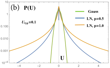
In this paper we introduce a natural generalization of this model and show that it displays a much richer phase diagram and a more realistic behavior. In GRP model every site of the reference space (represented by a matrix index) is connected to every other site with the transition amplitude distributed according to the Gaussian law. Such model occurs as the effective description of the systems without internal structure, in which transition between resonance sites is due to a small number of hops, such as random energy model Smelyanskiy et al. (2020); Faoro et al. (2019). In more realistic models delocalization of the wave function is due to a long series of quantum transitions. Each transition has a random amplitude, so their product is characterized by the log-normal (LN) distribution, rather than the Gaussian one as in GRP model. Inspired by this argument in this paper we introduce and study the generalization of RP model in which the transition amplitude between sites has a small typical value, as in RP model, but with much wider, log-normal distribution function that we define in Section II (see Fig. 1(b)).

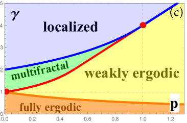
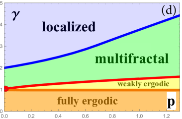
It appears that the rare large hopping matrix elements from the tail of this distribution alter the phase diagram of the system by considerably shrinking the region of multifractal phase as the parameter $p$ that controls the weight in the tail, increases. For large enough $p$ the multifractal phase is totally replaced by an ergodic one (see Fig. 1(c)). However, this ergodic phase is fragile. Because it is due to very rare hopping elements, even a far cutoff of the LN distribution function restores the multifractal phase and may even extend it in the phase diagram (Fig. 1(d)).

Generally, the mere statement that the eigenfunction fractal dimension $D_{1}=1$ is not sufficient for complete characterization of the ergodic phase. As was shown in Ref. Nosov et al. (2019), in certain translational-invariant RP models $D_{1}=1$ in the reference basis, yet in the Fourier-transformed ’momentum’ basis all eigenvectors are localized. Consequently, the eigenvalue statistics is Poisson, despite extended character of wave functions in the reference basis. On the other hand, the ergodic states in the GRP model remain ergodic in any basis von Soosten and Warzel (2018b), like in the classic Wigner-Dyson (WD) random matrix ensemble.

This observation urged us to distinguish between the fully-ergodic (FE) and the weakly-ergodic (WE) phases. In FE phase in the thermodynamic limit: ${\bf(i)}$ the eigenfunction statistics is Porter-Thomas, i.e. the fraction of essentially populated sites in an eigenfunction is $f=1$, ${\bf(ii)}$ the eigenvalue statistics is WD all the way to the bandwidth and ${\bf(iii)}$ eigenfunction statistics is invariant under basis rotation von Soosten and Warzel (2018b). In contrast, in WE phase  WE- this invariance is broken together with the emergence of the energy scale $\Gamma$ smaller than the bandwidth, beyond which the WD eigenvalue statistics breaks down and $f<1$ ( Fig. 1(a)). Furthermore, since the so defined two ergodic phases differ by the symmetry with respect to basis rotation, there should be a phase transition and not a crossover between them. We will refer to this transition between the fully- and weakly ergodic phases as the FWE transition. Note that the basis-rotation invariance von Soosten and Warzel (2018b) is not manifest present in the formulation of any RP model with a special diagonal. It is a non-trivial emergent symmetry which may arise only in the thermodynamic limit $N\rightarrow\infty$. We argue that the existence of FE phase is related to the absence of mobility edge: in systems with the mobility edge only WE phase may exist Khaymovich and Kravtsov (2020a). Indeed, the localized states at the edge of the spectrum should be orthogonal to extended states in the middle of the spectrum. This is only possible if the states in the middle of the spectrum have population holes, $f<1$ (see Fig.1(a)), exactly where the wave function coefficients of localized states at the spectral edge are peaked. The similar deviations from full ergodicity in generic many-body systems have been also explained it terms of the above orthogonality Haque et al. . An important example of a system where the mobility edge is known to be absent at small enough disorder Aizenman and Warzel (2011a) and which may be considered as a toy model for MBL De Luca et al. (2014), is the Anderson model on the Bethe lattice. We argue that the same is true for the models with long-range hopping, in particular for the LN-RP model  Khaymovich and Kravtsov (2020a).

The weakly-ergodic phase is much more widespread: for instance the metallic phase in 3D Anderson model is weakly-ergodic Kravtsov and Mirlin (1994); Fyodorov and Mirlin (1995). Due to the presence of the mobility edge the wave function coefficient distribution is not of the Porter-Thomas form Fyodorov and Mirlin (1995), while the level statistics at small energies is still WD in the thermodynamic limit Kravtsov and Mirlin (1994). A non-trivial feature of the LN-RP model is that both ergodic phases are present in it separated by a line of a new FWE quantum phase transition (see Fig. 1 (c)-(e)) similarly to the Bethe lattice Aizenman and Warzel (2011b).

Note that a critical point in the single-particle Anderson model in $d$ dimensions where the dimensionless conductance $g$ is size-independent, but no multifractality present, which was anticipated in  Bbrahams et al. (1979) and studied in Altshuler et al. (1994); Aronov et al. (1995), is surely weakly-ergodic but sub-diffusive: $\langle r^{2}\rangle\propto t^{2/d}$. It is probably similar kind of WE phase in the Hilbert space of interacting systems which is responsible for a so-called “bad metal” phase on the ergodic side of the localization transition. In such a phase, both many-body systems Luitz and Bar Lev (2016) and hierarchical structures like RRG Bera et al. (2018); De Tomasi et al. (2020) have been shown to demonstrate the anomalous sub-diffusive transport.

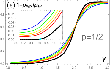
The analytical theory of the Ergodic (ET), Localization (AT), and FWE transitions developed in this paper is verified by extensive numerics based on the Kullback-Leibler divergence Kullback and Leibler (1951); Kullback (1959) of certain correlation functions ${\rm KL1}$ and ${\rm KL2}$ of wave function coefficients Pino et al. (2019) and on numerical investigation of the typical ($\rho_{{\rm typ}}$) and the mean ($\rho_{{\rm av}}$) Local Density of States (LDoS). The quantity $\phi=1-\rho_{{\rm typ}}/\rho_{{\rm av}}$ is an order parameter for the FWE transition, with $\phi=0$ in FE phase and $\phi>0$ in WE phase (see Fig. 1 (e)), while the onset of divergence (with the system size $N$) of ${\rm KL1}$ and ${\rm KL2}$ marks the AT and ET transitions, respectively (see Fig. 4).

II Log-Normal Roseizweig-Porter model

We introduce a modification of the RP random matrix ensemble Rosenzweig and Porter (1960); Kravtsov et al. (2015) in which the Gaussian distribution of independent, identically distributed (i..i.d.) off-diagonal real entries $H_{nm}=U$ is replaced by the logarithmically-normal one:

$$P(U)=\frac{A}{|U|}\,{\rm exp}\left[-\frac{\ln^{2}(|U|/U_{{\rm typ}})}{2p\,\ln(U_{{\rm typ}}^{-1})}\right],\;\;U_{{\rm typ}}\sim N^{-\gamma/2}.$$ (1)

It is characterized by two parameters: the disorder-parameter $\gamma$ which determines the scaling of the typical off-diagonal matrix element with the matrix size $N$ and the parameter $p$ that controls the weight of the tail.

The i.i.d. diagonal entries are supposed to remain Gaussian distributed, as in the original RP model:

$$\langle H_{nn}\rangle=0,\;\;\;\langle H_{nn}^{2}\rangle=W^{2}\sim N^{0}.$$ (2)

This LN-RP model is principally different from the Lévy random matrix models (see, e.g., Cizeau and Bouchaud (1994); Tarquini et al. (2016); Cao et al. (2017) and references therein) exactly because the Gaussian distribution (2) is not tailed. For numerical purposes we will replace it by the box distribution which is plain in the interval $[-W/2,W/2]$.

The tailed distribution (1) gives rise to the moments $\langle|U|^{q}\rangle^{\frac{1}{q}}\sim N^{-\gamma_{q}/2}$ that scale differently with $N$ for different values of $q$:

$$\gamma_{q}=\gamma\,(1-pq/2).$$ (3)

The limit $p\rightarrow 0$ in which $\gamma_{q}=\gamma$, corresponds to the GRP model. It is shown in Ref. Kravtsov et al. that $p=1$ is associated with RRG due to the hidden $\beta$-symmetry on the local Cayley tree (see Eqs. (6.5)-(6.8) in Ref. Abou-Chacra et al. (1973), Eqs. (D.2), (D.17) in Ref. V.E.Kravtsov et al. (2018) and Appendix C in Ref. Kravtsov et al. ). Finally, the limit $p\rightarrow\infty$ corresponds to the Lévy power-law distribution of $U$ Tarzia and Biroli (2020).

For any physically meaningful quantity in the bulk of the spectrum with a bandwidth $E_{BW}$, only the values $|U|<E_{BW}$ are relevant. For larger values of $|U|=|H_{nm}|$ the states are pushed to the Lifshits tails of the spectrum which we are not interested in this paper. As in the non-ergodic part of phase diagram $E_{BW}\sim W$ is of the order of the spread of on-site energies, in these regimes the distribution $P(U)$ is effectively cut off for $|U|>W$. However, for ergodic states $E_{BW}$ is determined by the off-diagonal matrix elements and is divergent with $N$. In this case the effective cutoff $E_{BW}$ in (1) should be determined self-consistently  del .

III Criteria of Localization, Ergodic and FWE transitions for dense random matrices

In this section we consider simple criteria of the disorder-driven  localization, ergodic and FWE transitions for random $N\times N$ matrices with the random uncorrelated random hopping $\langle H_{nm}\rangle=0$ and diagonal disorder $\sim O(1)$. More general picture and examples of systems are presented in Refs. Bogomolny and Sieber (2018); Nosov et al. (2019).

The first criterion, which is referred to as the Anderson localization criterion, states that if the sum :

$$S_{1}=\sum_{m=1}^{N}\langle|H_{n,m}|\rangle_{0}=N\,\langle|U|\rangle_{0},$$ (4)

goes to zero in the limit $N\rightarrow\infty$ then the states are Anderson localized, while if the above sum diverges the states are surely delocalized. The case $S_{1}=O(1)$ which is relevant for the short-range, size-independent random Hamiltonians (e.g.for the 3D Anderson model), is system- specific.

Here $\left\langle..\right\rangle_{0}$ stands for the disorder averaging over the distribution, (1), which is cut off at $|U|>W\sim N^{0}$. The reason for such a cutoff is the following. The physical meaning of (4) is that the number is sites in resonance with a given site $n$ is finite. The probability that two sites $n$ and $m$ are in resonance is:

$$P_{n\rightarrow m}=\int\limits_{-W/2}^{W/2}\frac{d\varepsilon_{n}}{W}\int\limits_{-W/2}^{W/2}\frac{d\varepsilon_{m}}{W}\int\limits_{|\omega|}^{\infty}\,P(H_{nm})\,d(H_{nm}),$$ (5)

where for simplicity we consider the box-shaped distribution $F(\varepsilon)$ of on-site energies. Then integration over $(\varepsilon_{n}+\varepsilon_{m})/2$ and integration by parts over $\omega=\varepsilon_{n}-\varepsilon_{m}$ gives:

$$P_{n\rightarrow m}=\int\limits_{-W}^{W}dU\,P(U)\,\left(\frac{|U|}{W}-\frac{U^{2}}{2W^{2}}\right)+\int\limits_{W}^{\infty}P(U)\,dU.$$ (6)

One can easily see that at $U_{{\rm typ}}\sim N^{-\gamma/2}\ll O(1)$ the last integral in (6) can always be neglected. The values of $|U|$ involved in the first integral are bounded from above $|U|<W$, which is equivalent to imposing a cutoff at $|U|>W$ on the distribution $P(U)$. As the second term in this integral is at most 1/2 of the first term, the number of sites in resonance with the given site, $\sum_{m}P_{n\rightarrow m}$, coincides with  (4) up to a pre-factor of order $O(1)$.

The second criterion referred to as the the Mott’s criterion is a sufficient criterion of ergodicity. It states that if the sum

$$S_{2}=\sum_{m=1}^{N}\langle|H_{nm}|^{2}\rangle_{E_{BW}}=N\,\langle U^{2}\rangle_{E_{BW}}\rightarrow\infty$$ (7)

diverges in the limit $N\rightarrow\infty$ then the system is in the one of the ergodic phases Nosov et al. (2019).

In Eq.(7) the subscript $E_{BW}$ implies that the distribution, Eq.(1) should be truncated at $U\sim E_{BW}$, where $E_{BW}\sim W\sim N^{0}$ is the total spectral bandwidth in the non-ergodic phase. The physical meaning of (7) is that the mean Breit-Wigner width $\Gamma\sim E_{BW}^{-1}\,N\langle U^{2}\rangle_{E_{BW}}$ SM that quantifies the escape rate of a particle created at a given site $n$, is much larger than the spread of energy levels $W\sim N^{0}$ due to disorder. Then the fulfillment of the Mott’s criterion implies that the width $\Gamma$ is of the same order as the total spectral bandwidth $E_{BW}\sim\sqrt{S_{2}}$ and thus there are no mini-bands (which width is $\Gamma$) in the local spectrum (see Fig. 1(a)). As the presence of such mini-bands is suggested Pino et al. (2017); De Tomasi et al. (2019); Nosov and Khaymovich (2019) as a “smoking gun” evidence of the non-ergodic extended (e.g. multifractal) phase, the fulfillment of the Mott’s criterion (7) immediately implies that the system is in the ergodic extended phase.

The multifractal phase realizes provided that in the limit $N\rightarrow\infty$ both (4) and (7) are not fulfilled:

$$S_{1}\rightarrow\infty,\;\;\;S_{2}<\infty.$$ (8)

Finally, the fully ergodic phase is realized when $S_{1},S_{2}\rightarrow\infty$ and also:

$$S_{3}=\frac{\left(\sum_{m=1}^{N}\langle|H_{nm}|^{2}\rangle_{{\rm typ}}\right)^{2}}{\sum_{m=1}^{N}\langle|H_{nm}|^{2}\rangle_{E_{BW}}}=\frac{N\,U_{{\rm typ}}^{4}}{\langle U^{2}\rangle_{E_{BW}}}\rightarrow\infty,$$ (9)

is divergent in the $N\rightarrow\infty$ limit, where $\langle|H_{nm}|^{2}\rangle_{{\rm typ}}\equiv U_{{\rm typ}}^{2}={\rm exp}\langle\ln|H_{nm}|^{2}\rangle$ E_B . If only $S_{1},S_{2}\rightarrow\infty$ but $S_{3}$ is not, the weakly ergodic phase is realized.

The physics behind the condition Eq.(9) is that the typical escape rate $\Gamma_{{\rm typ}}\sim E_{BW}^{-1}\,N\,U_{{\rm typ}}^{2}=\sqrt{S_{3}}$ SM is much larger than the disorder strength $W\sim N^{0}$. The two conditions, Eqs.(7),(9), coincide for a Gaussian distribution of $U$ but are different for the tailed ones, like LN distribution, Eq.(1).

IV Phase diagram

For the log-normal distribution (1) one easily computes the moments $\left\langle|U|^{q}\right\rangle_{0}$ truncated at $U_{{\rm max}}\sim N^{0}$:

$$\langle U^{q}\rangle_{0}=\left\{\begin{array}[]{ll}N^{-\frac{\gamma q}{2}\,\left(1-\frac{pq}{2}\right)},&{\rm if}\;\;pq<1\cr N^{-\frac{\gamma}{4p}},&{\rm if}\;\;pq\geq 1\end{array}\right.$$ (10)

and finds using (3), (4), (7), (9) and $U_{{\rm typ}}=N^{-\gamma/2}$ the following critical points of the localization ($\gamma_{AT}$), ergodic ($\gamma_{ET}$) and FWE ($\gamma_{FWE}$) transitions:

$$\gamma_{AT}=\left\{\begin{array}[]{ll}\frac{4}{2-p},&{\rm if}\;\;p<1\cr 4p,&{\rm if}\;\;p\geq 1\end{array}\right.$$ (11)

$$\gamma_{ET}=\left\{\begin{array}[]{ll}\frac{1}{1-p},&{\rm if}\;\;p<1/2\cr 4p,&{\rm if}\;\;p\geq 1/2\end{array}\right.$$ (12)

$$\gamma_{FWE}=\frac{1}{1+p}.$$ (13)

The phase diagram at a fixed energy in the middle of spectrum resulting from  (11)-(13), is presented in Fig. 1(c).

The main conclusion we may draw from this phase diagram is the emergence and proliferation of the weakly-ergodic phase that pushes away both the multifractal (MF) phase and the fully ergodic phase, as the strength of the tail $p$ in the distribution  (1) increases. For $p>1$ the MF phase is completely gone replaced by the weakly ergodic one. However, this WE phase is fragile. Truncation of the tail of this distribution, so that $|U|<N^{-\gamma_{{\rm tr}}}$, $\gamma_{{\rm tr}}>0$, eliminates the WE phase and restores the MF phase, as well as increases the range of the fully-ergodic one (see Fig. 1(d) and Appendix A for details).

V Stability of non-ergodic states against hybridization

Figure 2: (Color online) Hybridization of fractal support sets (a), (b) Two different fractal support sets, (c) The hybridized fractal support set.

In this section we consider the stability of non-ergodic (multifractal and localized) states against hybridization. It allows us not only to derive expressions, (4) and (7), for the Anderson localization and ergodic transitions in a different way but also find the fractal dimension $D_{1}(p,\gamma)$ of the multifractal support set. The fractal dimension $D_{1}$ plays a special role, because it gives the scaling of the volume $N^{D_{1}}$ of the support set of wave functions with the total system volume $N$ De Luca et al. (2013). The fundamental role of the support set is that it gives the number of sites in the reference space and the number of states in the energy space that is minimally sufficient for the normalization and completeness conditions. As a consequence, $D_{1}$ is directly related to the spectrum of fractal dimensions $f(\alpha)$ via $D_{1}=\alpha_{1}=f(\alpha_{1})$ which significantly simplifies the analysis presented below. Furthermore, the new method presented below is physically transparent and generic enough to be applied to analysis of the multifractal states in other systems.

Figure 3: (Color online) The functions (24)(blue curve) and (25) (orange curve) entering inequalities  (22), (23) in different regions of $p$: (a) $p<1/2$; (b) $1/2\leq p\leq 1$; (c) $p>1$. Intervals of $\alpha=D_{1}/\gamma$ with different functional dependence are shown by dashed vertical lines. The Anderson localization transition corresponds to the lower of the blue and orange curves equal to $2/\gamma$ at $\alpha=0$. This transition is always determined by the orange curve representing the log-normal part of the distribution $P(V)$. On the contrary, the stable fractal dimension $D_{1}(\gamma)=2-\gamma/\gamma_{ET}(p)$ for $\gamma\leq\gamma_{AT}$ is always determined by the blue curve representing the Gaussian part of the distribution $P(V)$. The Anderson transition in all cases but $p=0$ is characterized by the minimal stable fractal dimension of the support set being $D^{{\rm min}}_{1}=D_{1}(\gamma_{AT})=2-\gamma_{AT}/\gamma_{ET}(p)>0$ (shown by a gray dotted arrow). The ergodic transition corresponds to $D_{1}(\gamma)=1$ and it is continuous. For $p\geq 1$ there is no solution $D_{1}<1$ to the system of inequalities (22), (23) in the region of parameters where the localized phase is unstable. In this case the multifractal phase is absent.

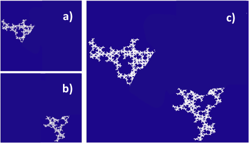
Let us consider two states $\psi_{\mu}$ and $\psi_{\nu}$ on different fractal support sets as it is shown in Fig. 2(a) and (b). We assume that both states are multifractal with $m\sim N^{D_{1}}$ sites on a fractal support set where the coefficients $|\psi(i)|^{2}\sim N^{-D_{1}}$.

Here we apply a usual Mott’s argument for hybridization of states, Fig. 2(c), when the disorder realization, in this case the off-diagonal matrix element, changes from $H_{ij}$ to $H_{ij}^{\prime}=H_{ij}+\delta\,H_{ij}$. The key new element in the theory we are introducing here is the hopping matrix element $V_{\mu,\nu}$ between the states and not between the sites as is customary:

$$V_{\mu,\nu}=\sum_{i,j}\delta\,H_{ij}\,\psi_{\mu}(i)\,\psi_{\nu}(j).$$ (14)

Here $\psi_{\mu}(i)$ is the eigenfunction of the $\mu$-th state of $H_{ij}$, and $\delta\,H_{ij}=H_{ij}^{\prime}-H_{ij}$, where $H_{ij}^{\prime}$ is drawn from the same log-normal distribution as $H_{ij}$.

Introducing $g_{ij}=-\ln\delta\,H_{ij}/\ln N$ and suppressing the indices $i,j$ for brevity we conveniently rewrite (1) as follows :

$${\cal P}(g)={\rm const}\,N^{-\frac{1}{p\gamma}\,\left(g-\frac{\gamma}{2}\right)^{2}},\;\;\;(g\geq 0).$$ (15)

By the constraint $g\geq 0$ we implemented the cutoff at $|U|\sim O(N^{0})$ discussed in Sec. III.

The typical number of terms in the sum (14) in the interval $dg$ is $N^{D_{1}}N^{D_{1}}{\cal P}(g)\sim N^{\sigma(g,D_{1})}\,dg$ where

$$\sigma(g,D_{1})=2D_{1}-\frac{1}{p\gamma}\,\left(g-\frac{\gamma}{2}\right)^{2}.$$ (16)

If $\sigma(g,D_{1})<0$, the sum, (14), is dominated by a single term with the largest $|G_{ij}|$. For positive $\sigma(g,D_{1})>0$, many terms contribute to this sum and the distribution $P(V\equiv|V_{\mu,\nu}|)$ becomes Gaussian. In general, there are both contributions

$$P(V)=P_{{\rm LN}}(V)+P_{{\rm Gauss}}(V).$$ (17)

The condition of stability of the multifractal phase against hybridization is derived similar to the Anderson criteria of stability, (4), of the localized. The difference is that now we have to replace the matrix element between the resonant sites $U$ by the matrix element $V$ between the resonant non-ergodic states and take into account that on each of $M=N^{1-D_{1}}$ different support sets there are $m=N^{D_{1}}$ wave functions which belong to the same mini-band and thus are already in resonance with each other. Therefore the total number of independent states-candidates for hybridization with a given state should be smaller than the total number of states $M\,m=N$ and larger than the number of support sets $M$. This number is in fact equal to their geometric mean $\sqrt{NM}=M\,\sqrt{m}=N^{1-\frac{D_{1}}{2}}$.

With this comment, the criterion of stability of the multifractal phase reads in the limit $N\rightarrow\infty$ as

$$N^{1-\frac{D_{1}}{2}}\int\limits_{0}^{W}dV\,V\,P(V)<\infty\ .$$ (18)

The contribution of the Gaussian part $P_{{\rm Gauss}}$ in (17) to (18) is:

$$N^{1-\frac{D_{1}}{2}}\,\sqrt{\langle V^{2}\rangle}=N^{1-\frac{D_{1}}{2}-\frac{1}{2}\gamma_{{\rm eff}}(D_{1})}<\infty,$$ (19)

where

$$\langle V^{2}\rangle\equiv N^{-\gamma_{{\rm eff}}},$$ (20)

and for stability it must be finite as $N\rightarrow\infty$. The contribution of $P_{{\rm LN}}$ in (17) to the stability criterion (18) is
$N^{1-\frac{D_{1}}{2}-\frac{\Delta(D_{1})}{2}}<\infty$, where

$$\int\limits_{\sigma(g,D_{1})<0}dg\,N^{\sigma(g,D_{1})-g-D_{1}}\equiv N^{-\frac{\Delta(D_{1})}{2}}\ .$$ (21)

Thus the multifractal phase is stable against hybridization if the following inequalities are both fulfilled

$$D_{1}+\gamma_{{\rm eff}}(D_{1}) \geq 2,$$ (22)

$$D_{1}+\Delta(D_{1}) \geq 2.$$ (23)

The functions $\gamma_{{\rm eff}}(D_{1})$ and $\Delta(D_{1})$ are computed in Appendix B and discussed in the next Section.

A particular case $D_{1}=0$ of (22), (23) describes the stability criterion of the localized phase. If the localized phase is not stable, then hybridization produces an avalanche of multifractal states living on fractal support which dimensionality grows until inequalities  (22), (23) are both fulfilled for the first time at some $0<D_{1}^{{\rm min}}<1$. If this is possible in some parameter region then the multifractal state is stable, otherwise the only stable extended phase is ergodic.

VI Fractal dimension of the NEE support set

In this section we re-consider the phase diagram Fig. 1(c) from the viewpoint of stability criteria given in the previous section by (22),  (23) and derive the expression for the fractal dimension $D_{1}(\gamma)$.

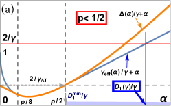
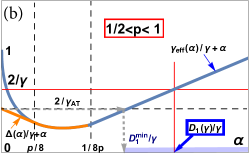
To this end in Fig. 3 we plot

$$\frac{\gamma_{{\rm eff}}(\alpha)}{\gamma}+\alpha=\left\{\begin{array}[]{ll}1+3\alpha-2\sqrt{2\alpha p},&4\alpha<2p,\frac{1}{2p}\\ 1/\gamma_{ET}(p)+\alpha,&\text{otherwise}\end{array}\right.\ ,$$ (24)

and

$$\frac{\Delta(\alpha)}{\gamma}+\alpha=\left\{\begin{array}[]{ll}1+3\alpha-2\sqrt{2\alpha p},&p<8\alpha<\frac{1}{p}\\ {2}/{\gamma_{AT}(p)}-\alpha,&8\alpha<p,\frac{1}{p}\\ 1+3\alpha+2\sqrt{2\alpha p},&8\alpha>\frac{1}{p}\end{array}\right.\ ,$$ (25)

as functions of $\alpha=D_{1}/\gamma$. Here $\gamma_{AT}(p)\geq 2$ and $\gamma_{ET}(p)\geq 1$ are given by (11) and (12), respectively (the details of derivation of  (24), (25) from (20), (21) are presented in Appendix B).

Figure 4: (Color online) Plots of ${\rm KL1}$ and ${\rm KL2}$ vs. $\gamma$ for LN-RP model at $N=2^{L}$, with $L$ from $9$ to $15$ with the step $1$ (from red to violet). The logarithmic in $N$ divergence of ${\rm KL1}$ for $\gamma>\gamma_{AT}\approx 2$ and of ${\rm KL2}$ for $\gamma>\gamma_{ET}\approx 1$ is demonstrated in a wide interval of $\gamma$ for $p=0.01$, as well as insensitivity of ${\rm KL1}$ to the ergodic transition. Intersection for ${\rm KL2}(\gamma$) curves is sharp at the isolated continuous ergodic transition at $\gamma_{ET}\approx 1$ for $p=0.01$ and at $\gamma_{ET}\approx 2.1$ for $p=0.5$, it is smeared out for $p=1.0$ when the ergodic transition merges with the localization transition. Intersection of curves for ${\rm KL1}$ at the Anderson localization transition ($\gamma_{AT}\approx 2.0$ for $p=0.01$, $\gamma_{AT}\approx 2.8$ for $p=0.5$, $\gamma_{AT}\approx 4.1$ for $p=1$ ) is sharp in all the cases. The insets show the collapse of the curves at the proper choice of $\gamma_{c}$ and the critical exponents $\nu_{1}$ and $\nu_{2}$ for ${\rm KL1}$ and ${\rm KL2}$ at the AT and ET, respectively. The plot Fig.4(g) presents the simplest conjecture for $\nu_{1}$ and $\nu_{2}$ vs. $p$ consistent with the results of finite-size scaling presented in Table 1 and shown on the plot. In the limit $p\to 0$ the critical exponents approach their values $\nu_{1}=\nu_{2}=1$ for the Gaussian RP model Pino et al. (2019). For $p\geq 1$ we conjecture the mean-field values $\nu_{1}=\nu_{2}=1/2$.

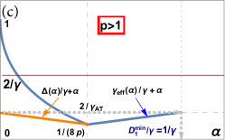
According to the stability criteria (22), (23) the functions (24), (25) should be compared to $2/\gamma$, see Fig. 3. First, we note that the localized phase which formally corresponds to $D_{1}=0$, is stable if the lowest of the blue and orange curves in Fig. 3 is higher than $2/\gamma$ at $\alpha=0$ and it is unstable otherwise. One can see that at $\alpha=0$ for all values of $p$ the log-normal contribution to (17) (orange curve) is lower than the Gaussian one (blue curve). This means that the stability of the localized phase is always determined by the log-normal part of $P(V)$. Moreover, since at $\alpha=0$  (24), (25) reduce to $\alpha+{\gamma_{{\rm eff}}(\alpha)}/{\gamma}=1$ and $\alpha+\Delta(\alpha)/\gamma=2/\gamma_{AT}$, respectively, the stability of the localized phase implies that $\gamma>\gamma_{AT}(p)\geq 2$ in agreement with (11).

If the localized phase is unstable then different localized states hybridize and form a multifractal state with $D_{1}>0$. Those states are, however, unstable until their support set reaches the fractal dimension $D_{1}^{min}>0$ where (22),  (23) are both fulfilled for the first time.

As the parameter $\gamma$ decreases below the critical value $\gamma_{AT}$, the stable fractal dimension $D_{1}(\gamma)$ increases from $D^{{\rm min}}_{1}$ being always determined by the intersection of the horizontal line $y=2/\gamma>2/\gamma_{AT}(p)$ (red line in Fig. 3) with the blue line. Thus the stable fractal dimension $D_{1}(\gamma)$ is always determined by the Gaussian part of $P(V)$ and according to the second line of (24) and Fig. 3 is equal to:

$$D_{1}(\gamma)=2-\gamma_{{\rm eff}}=2-\frac{\gamma}{\gamma_{ET}(p)}\ ,\quad p\leq 1\ .$$ (26)

At $\gamma=\gamma_{ET}$ the fractal dimension $D_{1}(\gamma)$ reaches unity, and at this point a continuous ergodic transition happens. Thus the critical point of ergodic transition coincides with that determined by (12).

Note that, unlike the ergodic transition, the localization transition is characterized by a jump in the fractal dimension $D_{1}$ between the multifractal and the localized phase (where $D_{1}=0$). The stable fractal dimension $D_{1}(\gamma)$ is non-zero just below the transition and is equal to:

$$D_{1}^{min}=\left\{\begin{array}[]{ll}2-\frac{\gamma_{AT}(p)}{\gamma_{ET}(p)},&0<p<1\cr 1,&p\geq 1\end{array}\right.$$ (27)

Figure 5: (Color online) Derivative of ${\rm KL2}$ w.r.t. $\ln N$ vs. $\gamma$ for LN-RP model extrapolated from pairs of sizes $N=512~{}-~{}16384$ (red solid lines) for (a) $p=0.01$ and (b) $p=0.5$ with the theoretical predictions (32) and (33) (grey dashed lines). The jump is related to the jump in $D_{1}$, (27), for all $p>0$. At $p\rightarrow 0$ the minimal fractal dimension $D_{min}\rightarrow 0$ and instead of the jump in the function $d{\rm KL2}/d\ln N$ vs. $\gamma$ there is only a jump in its $\gamma$-derivative at the AT. At $p=1/2$ and a at finite $N$, instead, the jump manifests itself in the dramatic increase of slope near $\gamma=\gamma_{AT}$.

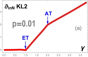
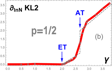
This minimal fractal dimension of the support set is shown by the gray dotted arrow in Fig. 3. As we show in the next section it reveals itself in the slope of the Kullback-Leibler divergence, see Fig. 5 and (32). Fig. 3(c) demonstrates that for $p\geq 1$ the minimal fractal dimension $D_{1}^{min}=1$, so that the multifractal phase is no longer possible in LN-RP model (1). However, it is restored if the LN distribution is truncated at $|U|\sim N^{-\gamma_{{\rm tr}}}$ with $\gamma_{{\rm tr}}>0$ (see Appendix A for details).

VII Kullback-Leibler (KL) measure

The numerical verification of (11), (12) and determination of the critical exponents at the Anderson localization and ergodic transitions is done in this paper using the Kullback-Leibler divergence (KL) Kullback and Leibler (1951); Kullback (1959); Luitz et al. (2015); Pino et al. (2019) .

The Kullback-Leibler correlation functions ${\rm KL1}$ and ${\rm KL2}$ are defined as follows  Luitz et al. (2015); Pino et al. (2019). The first one is defined in terms of wave functions of two neighboring in energy states $\psi_{\mu}(i)$ and $\psi_{\mu+1}(i)$ at the same disorder realization:

$${\rm KL1}=\left\langle\sum_{i}|\psi_{\mu}(i)|^{2}\,\ln\left(\frac{|\psi_{\mu}(i)|^{2}}{|\psi_{\mu+1}(i)|^{2}}\right)\right\rangle.$$ (28)

The second one is similar but the states $\psi$ and $\tilde{\psi}$ correspond to different (and totally uncorrelated) disorder realizations:

$${\rm KL2}=\left\langle\sum_{i}|\psi(i)|^{2}\,\ln\left(\frac{|\psi(i)|^{2}}{|\tilde{\psi}(i)|^{2}}\right)\right\rangle.$$ (29)

The idea to define such two measures is the following. In the ergodic phases each of the states has an amplitude $|\psi(i)|^{2}\sim N^{-1}$ of the same order of magnitude. Then the logarithm of their ratio is of order $O(1)$, and for the normalized states

$${\rm KL1}\sim{\rm KL2}\sim O(1).$$ (30)

For fully-ergodic states the eigenfunction coefficients are fully uncorrelated, even for the neighboring in energy states. Thus there is no difference between ${\rm KL1}$ and ${\rm KL2}$. Using the Porter-Thomas distribution one finds:

$${\rm KL1}={\rm KL2}=2.$$ (31)

For weakly-ergodic states ${\rm KL2}$ is still $O(1)$ but is larger than the Porter-Thomas value due to the fact that there are ’population holes’ where $N|\psi(i)|^{2}$ is $N$-independent but small, Fig. 1(a).

Deeply in the localized phase $\ln|\psi_{\mu}(i)|^{2}\sim-|i-i_{\mu}|/\xi$, where $i_{\mu}$ is the position of the localization center. Since the positions of localization centers $i_{\mu}$ are not correlated even for the states neighboring in the energy, the logarithm of the ratio of the two wave function coefficients in (28), (29) is divergent in the thermodynamic limit. For Anderson localized states on finite-dimensional lattices this divergence is linear in the system size $L$. However, localization on graphs such as RRG and RP models is not a conventional localization De Luca et al. (2014); Kravtsov et al. (2015). In this case there is a power-law in $1/N$ background with the most probable (typical) value of $|\psi(i)|^{2}_{{\rm typ}}\sim N^{-\alpha_{0}}$ far from the localization center and therefore:

$${\rm KL1}\sim{\rm KL2}=\alpha_{0}\,\ln N\rightarrow\infty$$ (32)

with $\alpha_{0}=(\gamma_{AT}/2)(\gamma-\gamma_{AT})+2$ for LN-RP model.

A qualitative difference between ${\rm KL1}$ and ${\rm KL2}$ is in the multifractal phase. In this phase the neighboring in energy states $|\psi_{\mu}(i)|^{2}$ and $|\psi_{\mu+1}(i)|^{2}$ are most probably belonging to the same support set MBL and hence they are strongly overlapping: $|\psi_{\mu}(i)|^{2}\sim|\psi_{\mu+1}(i)|^{2}$. Furthermore, eigenfunctions on the same fractal support set can be represented as: $\psi_{\mu}(i)=\Psi(i)\,\phi_{\mu}(i)$, where $\Psi(i)$ is the multifractal envelope on the support set and $\phi_{\mu}(i)$ is the fast oscillating function with the Porter-Thomas statistics De Luca et al. (2014). Thus the ratio $|\psi_{\mu}(i)|/|\psi_{\mu+1}(i)|$ and hence ${\rm KL1}$ in MF phase has the same statistics as in the ergodic one. We conclude that ${\rm KL1}$ is not sensitive to the ergodic transition but is very sensitive to the localization one, Fig. 4.

In contrast, the eigenfunctions $\psi(i)$ and $\tilde{\psi}(i)$ in ${\rm KL2}$ corresponding to different realizations of a random Hamiltonian, overlap very poorly in MF phase. This is because the fractal support sets which contain a vanishing fraction of all the sites, do not typically overlap when taken at random. Therefore

$${\rm KL2}=(\alpha_{0}-D_{1})\,\ln N=2(1-D_{1})\,\ln N$$ (33)

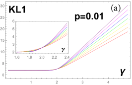
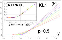
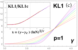
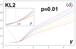
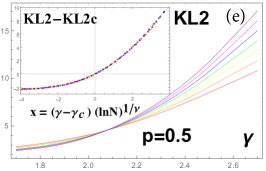
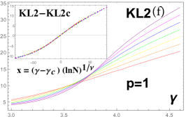
is divergent in the thermodynamic limit in the multifractal phase of RP models, with $(\alpha_{0}-D_{1})=2(\gamma/\gamma_{ET}-1)>0$, (26), very much like in the localized one. This makes ${\rm KL2}$ very sensitive to the ergodic transition. The properties of ${\rm KL1}$ and ${\rm KL2}$,  (31), (32), are fully confirmed by numerics presented in Fig. 4. The jump in the slope $\alpha_{0}(\gamma_{AT}+0)-\alpha_{0}(\gamma_{AT}-0)+D_{1}^{min}=2D_{1}^{min}$ at the Anderson transition, $\gamma=\gamma_{AT}$, originates from the jump in $D_{1}$, (27). Numerically it is clearly seen in the derivative of KL2 over $\ln N$ versus $\gamma$ shown in Fig. 5. We also show in Fig. 6 that ${\rm KL2}$ is sensitive to the FWE transition and can be operative in identifying it.

A more detailed theory of ${\rm KL1}$ and ${\rm KL2}$ in the multifractal phase is given in Appendix C. The main conclusion of this analysis is that the curves for ${\rm KL1}(\gamma,N$) for different $N$ have an intersection point at the critical point $\gamma=\gamma_{AT}$ of the Anderson localization transition. At the same time, the intersection point for curves for ${\rm KL2}(\gamma,N$) coincides with the ergodic transition Pino et al. (2019), provided that it is continuous and well separated from the Anderson localization transition. If the localization and ergodic transition merge together and the multifractal state exists only at the transition point, then intersection of ${\rm KL2}$ curves is smeared out and may disappear whatsoever (as in 3D Anderson model). However, the intersection of ${\rm KL1}$ curves remains sharp in this case too (see Fig. 4).

p	$\gamma_{AT}$	$\{ext\}$, $[th]$	$\gamma_{ET}$	$\{ext\}$, $[th]$	$\nu_{1}$	$\nu_{2}$
$0.01$	$2.00$	$[2]$	$1.00$	$[1]$	$1.02\pm 0.03$	$0.98\pm 0.05$
$1/2$	$2.80$	$[2.67]$	$2.06$	$[2]$	$0.70\pm 0.07$	$1.18\pm 0.15$
$3/4$	$3.43$	$[3.2]$	$2.96$	$[3]$	$0.64\pm 0.07$	$0.79\pm 0.12$
$1$	$4.10$	$\{4.04\}$, $[4]$	$3.90$	$\{4.10\}$, $[4]$	$0.56\pm 0.07$	$0.48\pm 0.08$
$5/4$	$4.81$	$\{5.02\}$, $[5]$	$4.45$	$\{5.19\}$, $[5]$	$0.57\pm 0.08$	$0.50\pm 0.10$
$3/2$	$5.51$	$\{5.84\}$, $[6]$	$5.18$	$\{5.83\}$, $[6]$	$0.57\pm 0.10$	$0.46\pm 0.10$

Table 1: Comparison of analytical predictions (blue), (11), (12), and numerical data for the transition points $\gamma_{AT}$ and $\gamma_{ET}$ and the corresponding critical exponents $\nu_{1}$ and $\nu_{2}$ for LN-RP model. Numerical data (black) is obtained by exact diagonalization of LN-RP random matrices with $N=512-32768$ from the intersection points in ${\rm KL1}$ and ${\rm KL2}$ and from finite-size scaling by the best collapse of the curves, Fig. 4. For $p>1$ a linear in $1/\ln N$ extrapolation to $N\rightarrow\infty$ of the position of the intersection point for two consecutive $N$ is shown in red.

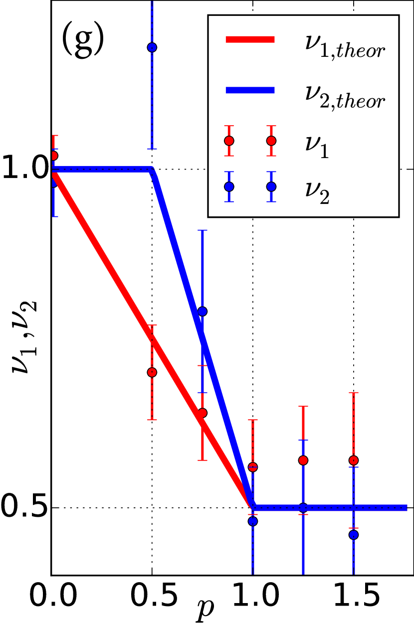
The intersection of finite-size curves for ${\rm KL1}$ and ${\rm KL2}$ helps to locate numerically the critical points $\gamma_{AT}$ and $\gamma_{ET}$. More precise determination of the critical points and the corresponding critical exponents $\nu_{1}$ and $\nu_{2}$ is done by the finite-size scaling (FSS) data collapse (see insets in Fig. 4 and Appendix D). The results are shown in the Table  1. On the basis of these numerical results we conclude that our expressions (11), (12) for the Anderson and ergodic transition points are accurate and conjecture on the $p$-dependence of the critical exponents $\nu_{1}$ and $\nu_{2}$ of AT and ET obtained from ${\rm KL1}$ and ${\rm KL2}$. (see Fig. 4(g)).

VIII Numerical location of the FWE transition

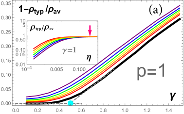
For numerical verification of (13) for FWE transition point we make use of the ratio of the typical $\rho_{{\rm typ}}$ and mean $\rho_{{\rm av}}$ average

$$\ln\rho_{{\rm typ}}=\left\langle\ln\rho(x,E+i\eta)\right\rangle\ ,\quad\rho_{{\rm av}}=\left\langle\rho(x,E+i\eta)\right\rangle\ ,$$ (34)

of local density of states (LDOS)

$$\rho(x,E+i\eta)={\rm\,Im\,}\sum_{\mu}|\psi_{\mu}(x)|^{2}/(E+i\eta-E_{\mu})\ .$$ (35)

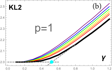
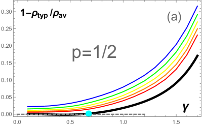
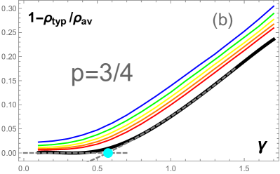
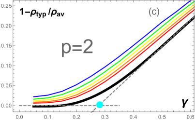
As is shown in Ref. V.E.Kravtsov et al. (2018), at small bare level width $\eta\ll E_{BW}/N$, where $E_{BW}=\max(\Gamma,W)$ is the total spectrum bandwidth, this ratio $\rho_{{\rm typ}}/\rho_{{\rm av}}\sim\eta\,N^{D_{1}}/E_{BW}$ grows linearly with $\eta$ but then saturates at $\rho_{{\rm typ}}/\rho_{{\rm av}}\sim N^{-1+D_{1}}$. In the ergodic phase $D_{1}=1$ and the plateau in $\rho_{{\rm typ}}/\rho_{{\rm av}}$ tends to a finite limit as $N\rightarrow\infty$. This behavior is well seen in the inset of Fig. 6. We used the properly defined plateau value of $\phi=1-\rho_{{\rm typ}}/\rho_{{\rm av}}$ as the order parameter for the FWE transition. For $\gamma<\gamma_{FWE}$ this parameter $\phi=0$, signaling of the fully-ergodic phase. For $\gamma>\gamma_{FWE}$ the order parameter is non-zero. This behavior is shown in Fig. 6 (see also an inset in Fig. 1(e) and figures in Appendix F), where the black curve represents $\phi=\phi_{\infty}(\gamma)$ extrapolated to $N=\infty$ from the finite $N$ values $\phi_{N}(\gamma)$ obtained by exact diagonalization. In spite of imperfect extrapolation that does not allow to get a true non-analyticity at $\gamma=\gamma_{FWE}$, the dashed gray lines of continuation of the black curve intersect exactly at $\gamma=1/2$ which is the predicted value of $\gamma_{FWE}$ at $p=1$. A similar intersection at $\gamma\approx 1/2$ is shown in the ${\rm KL2}$ vs. $\gamma$ plot in Fig. 6.They all suggest that the FWE transition does exist and is described by (13).

Figure 6: (Color online) (a): The ratio of the typical and average LDoS as a function of $\gamma$ for $p=1$ at different values of $N=512-32768$ (purple through red) and extrapolated to $N=\infty$ (black). Intersection of dashed lines gives the position of FE-WE transition point $\gamma_{FWE}\approx 0.5$ (shown by a bright blue point) as predicted by (13). Inset: dependence on the level width $\eta$. The main plot is done for $\eta$ shown by an arrow at the plateau of $\eta$-dependence. (b): The Zoom of Fig. 4(f) KL2 vs. $\gamma$ for p=1 for the same values of $N$ and their extrapolation to $N\rightarrow\infty$. Intersection of dashed lines gives the same position of FWE transition $\gamma_{FWE}\approx 0.5$ as on Fig.6(a).

Figure 7: (Color online)Fractal miniband structure. (a) The sketch of fractal set of fractal mini-bands in the local spectrum in the case when fractal dimension $D_{s,in}$ of the set of levels within a mini-band is larger than the fractal dimension $D_{s,out}$ of the set of mini-bands. The width of mini-bands $\Gamma$ tends to zero in the limit $N\rightarrow\infty$ while the number of levels $\Gamma/\delta$ in a mini-band tends to infinity; (b) The correlation function $K(\omega)$ for LN-RP model with $p=0.01$, $\gamma=1.5$, which corresponds to the eigenfunction fractal dimension $D_{2}\approx 2-\gamma=0.5$. $K(\omega)$ in this limit is almost indistinguishable from the one for GRP. It corresponds to a single Lorenzian mini-band with $D_{s,in}\rightarrow 1$ and is characterized by a single (trivial) power-law $K(\omega)\propto\omega^{-2}$. (c) $K(\omega)$ in the multifractal phase of LN-RP model with $p=0.5,\gamma=2.5$. It has a low-energy plateau which onset scales as $\omega\sim N^{-0.56}\gg N^{-1}$. It can be interpreted as the width a mini-band. At $\omega\rightarrow 0$ all plots collapse in one horizontal line after rescaling $N^{D_{2}}\,K(\omega)$, where $D_{2}\approx 0.5$ for (b) and $D_{2}\approx 0.30$ for (c). The falling part of $K(\omega)$ at larger $\omega$ cannot be described by a single power-law with a trivial exponent $\mu_{out}=2$. This is compatible with existence of extensive number of mini-bands with the fractal structure as shown in (a). In panels (b) and (c) the color code corresponds to $N=512$, $1024$, $2048$, $4096$, $8192$, $16384$ from purple to red. In the insets: the derivative $\mu(\omega)=-d\ln K(\omega)/d\ln\omega$ which gives a running with $\omega$ exponent of a local power-law. It demonstrates a formation of a plateau at $\mu\approx 1$ with increasing $N$. At large $\omega\sim E_{BW}$ a high-$\omega$ plateau emerges which level goes down towards $-2$ as $N$ increases. The correlation function $K(\omega)$ is a proxy for the correlation function of local operators $\int dt\,e^{i\omega t}\,\langle O(r,t)\,O(r,0)\rangle$ in the problem of many-body localization, e.g. the spin-spin correlation function Serbyn et al. (2017); Sels and Polkovnikov (2020).

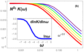
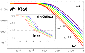
IX Fractal structure of mini-bands in the local spectrum.

In non-ergodic phases the spectral statistics of local operators differs drastically from its global counterpart. This is because in a given observation point many states have negligible amplitude in the limit $N\rightarrow\infty$ and thus cannot be seen. So emerges the pure-point spectrum in the localized phase. In the multifractal phase the hierarchical structure of distribution of wave function coefficients in the reference space imposes, due to completeness, the fractal structure of the local spectrum with power-law distribution of large inter-level spacing. Generically, both the distribution of levels inside a mini-band and the distribution of mini-bands in the local spectrum may have a fractal structure.

The simplest model of the local spectrum is shown in Fig.7(a). It consists of the set of mini-bands with the width $\Gamma$ that vanishes in the limit $N\rightarrow\infty$. Yet, in any of such mini-band there is an extensive number of levels, $\Gamma/\delta$, going to infinity in this limit, due to $\delta\ll\Gamma\ll E_{BW}$. This allows one to define the fractal dimension $D_{s,in}$ of the local spectrum inside a mini-band, as well as the fractal dimension $D_{s,out}$ of the set of mini-bands. The global spectrum is a union of such sets which pave densely all the spectral band. However, in each given observation point one can see a sparse set of mini-bands or even one single mini band, as in the GRP model. The same set of mini-bands can be seen in observation points which constitute a fractal support set in the reference space. There are many support sets which the reference space is divided into, each of them corresponding to a certain set of mini-bands. The stratification of the reference space first suggested in Cuevas and Kravtsov (2007) is a typical feature of the multifractal phase.

This qualitative picture can be tested by the correlation function $K(\omega)$ Cuevas and Kravtsov (2007):

$$K(\omega)=\frac{\sum_{n,m}\langle|\psi_{n}(r)|^{2}\,|\psi_{m}(r)|^{2}\delta(E-E_{n})\delta(E+\omega-E_{m})\rangle}{N^{-1}\sum_{n,m}\langle\delta(E-E_{n})\delta(E+\omega-E_{m})\rangle},$$ (36)

where $\psi_{n}(r)$ and $E_{n}$ is the eigenfunction coefficient and the eigenenergy of the $n$-th state.

One can show Pino et al. (2017); Khaymovich and Kravtsov (2020b) that the fractal spectrum like in Fig.7(a) leads to $K(\omega)$ which in the simplest approximation could be represented by two different power-laws in $\omega$. For $N^{-1}<\omega<\Gamma$ smaller than the width $\Gamma$ of a mini-band, the exponent $\mu_{in}$ of the power-law $K(\omega)\sim\omega^{-\mu_{in}}$ that reflects the fractal structure of spectrum inside a mini-band, is equal to $\mu_{in}=1-D_{s,in}$. For GRP where $D_{s,in}=1$, one finds a trivial value $\mu_{in}=0$ which just extends the low-$\omega$ plateau beyond its natural limit $\omega=N^{-1}$.

At larger $\omega\gg\Gamma$ the exponent $\mu_{out}$, reflecting the fractal structure of the set of mini-bands, can take any values $0\leq\mu_{out}\leq 2$. For the Gaussian RP, $K(\omega)$ is just a Lorenzian  Kravtsov et al. (2015); De Tomasi et al. (2019); Facoetti et al. (2016), and $\mu_{out}$ reaches its maximal value $\mu_{out}=2$. A similar behavior arises for LN-RP in the limit $p\rightarrow 0$ (see Fig.7(b)).

In the MF phase of LN-RP model with $0<p<1$ the exponent $\mu_{out}$ appears to be non-trivial  Khaymovich and Kravtsov (2020b), while $D_{s,in}$ is still equal to 1. A typical $K(\omega)$ is shown in Fig.7(c) obtained for $p=0.5$ and $\gamma=2.5$, $\gamma_{ET}<\gamma<\gamma_{AT}$ by exact diagonalization. The low-$\omega$ plateau corresponding to $\mu_{in}=0$ is terminated at $\omega\sim N^{-0.56}$. It is followed by the under-developed power law with $\mu_{out}\approx 1.2$. At yet larger $\omega\sim E_{BW}$ of the order of the total band-width, the slope of the log-log plot of $K(\omega)$ decreases towards $-2$. Note that the fact that the low-energy plateau is extended till $\omega\sim N^{-0.56}$ much greater than the mean level spacing $\sim N^{-1}$, tells us that the spectrum inside a mini-band of the width $\Gamma\sim N^{-0.56}$ has a fractal dimension $D_{s,in}=1$, as in the case of GRP. On the contrary, the complex behavior of $\mu(\omega)=-d\ln K(\omega)/d\ln\omega$ for $\omega>\Gamma$ which shows a shoulder at a non-trivial $\mu_{out}\approx 1.2$, signals of the fractal structure of the set of mini-bands.

Concluding this section, we would like to note that $K(\omega)$ can be considered as a proxy for the correlation function of a local observable in many-body systems, e.g. the Fourier-transform of the spin auto-correlation function Biroli and Tarzia (2017). This quantity is very popular in the MBL literature Serbyn et al. (2017). In particular, it has been very recently studied in connection to the discussion of the true nature of the MBL phase Sels and Polkovnikov (2020).

X Conclusion and Discussion

In this paper we introduce a log-normal Rosenzweig-Porter (LN-RP) random matrix ensemble characterized by a long-tailed distribution of off-diagonal matrix elements. We obtain analytically the phase diagram of LN-RP using the Anderson localization and Mott ergodicity criteria for random matrices complemented by the new criterion for the transition between the fully- and weakly-ergodic phases. This phase diagram is confirmed it by extensive numerics.

An alternative approach to localization and ergodic transitions based on the analysis of stability with respect to hybridization of multifractal wave functions developed in this paper gives results identical to those obtained from the above criteria. Using this approach we computed analytically the dimension $D_{1}$ of the eigenfunction fractal support set and showed that the Anderson localization transition in our model is characterized by a jump in the fractal dimension $D_{1}$ with the minimal fractal dimension $D_{1}^{{\rm min}}>0$.

Our results show how the rare off-diagonal matrix elements which are much larger than the typical ones, give rise to a phase diagram with the fully-ergodic as well as a fragile weakly-ergodic and multifractal extended phases and a new FWE phase transition between the two ergodic phases. These results shed light on the nature of the extended states in the Anderson model on Random Regular Graph, as well as in the Hilbert space of interacting systems in the problem of Many-Body Localization.

Here we would like to mention the correspondence of the LN-RP model to a generic many-body localization problem. Similar to Tarzia (2020) starting from the short-range Hamiltonian of interacting particles in a many-body problem one can compute the parameters of the effective long-ranged LN-RP model. As the MBL phase breaks down the ergodicity and given the emerging evidence Macé et al. (2019) that the wave function in this phase has a multifractal structure in the Hilbert space, the MBL transition should be associated with the ergodic transition, $\gamma_{ET}$, of our model. The localization in the Hilbert space of a generic many-body system can be achieved only at the disorder strength $W$ scaling with the system size $L$ Giuseppe De Tomasi (2020), thus, $\gamma_{AT}$ corresponds to $W\sim L$. It is also tempting to associate the FWE transition at $\gamma=\gamma_{FWE}$ between the fully and the weakly ergodic phases discovered in this paper, with the diffusion - sub-diffusion transition in the many-body setting Luitz and Bar Lev (2016). However, this correspondence has limitations related with correlated nature of off-diagonal matrix elements in the Hilbert space due to the locality of Hamiltonian in the real space. Such correlations, as well as the notion of locality is absent in our model.

Appendix A Truncated LN-RP and fragility of ergodic phase.

The phase diagram shown in Fig. 1 of the main text confirmed numerically by calculations of the KL-divergence and by the ratio of typical and mean local density of states (LDOS) demonstrates the collapse of the multifractal phase at $p\geq 1$ and existence of the tricritical points in LN-RP model at $p=0$ and $p=1$.

In this section we show that the weakly-ergodic (WE) phase that emerges at $p>0$ and replaces fully the multifractal (MF) phase and partly the fully-ergodic (FE) one at $p\geq 1$ is unstable with respect to a deformation of LN-RP model such that $P(U)$ is cut from above at:

$$U_{\rm max}\sim N^{-\gamma_{tr}/2}\ll O(1),\;\;\;\;(\gamma_{tr}>0).$$ (37)

As the result of this truncation the multifractal phase re-appears by substituting a part of the ergodic phase in a non-truncated LN-RP model (see Fig. 1(d))  foo . To this end we use the expression that generalizes (10):

$$\int\limits_{0}^{\min(N^{-\gamma_{\rm tr}/2},W)}dU\,U^{q}\,P(U)\sim$$

$$\sim\left\{\begin{array}[]{ll}N^{-\frac{q\gamma}{2}\left(1-\frac{pq}{2}\right)},&\gamma(1-pq)>\gamma_{\rm tr},0\\ N^{-\frac{1}{p\gamma}\left[\frac{(\gamma-\gamma_{\rm tr})^{2}}{4}+\frac{1}{2}\,pq\,\gamma\gamma_{\rm tr}\right]},&\gamma_{\rm tr}>\gamma(1-pq),0\\ N^{-\frac{\gamma}{4p}},&\gamma_{\rm tr},\gamma(1-pq)<0\end{array}\right.$$ (41)

and apply the same criteria (4), (7), (9) to find the critical points of the localization and both ergodic transitions.

Then we obtain that the critical point $\gamma_{AT}$ of the Anderson localization transition is affected as follows

$$\gamma_{AT}=2p-(p-1)\gamma_{tr}+\sqrt{(2p-(p-1)\gamma_{tr})^{2}-\gamma_{tr}^{2}},$$ (42)

only if $\gamma_{tr}>\gamma_{AT}\,(1-p),0$. In the opposite case truncation does not affect $\gamma_{AT}$.

For the critical point $\gamma_{ET}$ of the ergodic transition in the same way we find the effect only for $\gamma_{tr}>\gamma_{ET}\,(1-2p),0$ given by

$$\gamma_{ET}=2p-(2p-1)\gamma_{tr}+\sqrt{(2p-(2p-1)\gamma_{tr})^{2}-\gamma_{tr}^{2}}.$$ (43)

The criterion for the fully-weakly ergodic (FWE) transition does not have any truncation of $\left\langle U^{2}\right\rangle$ at $U\sim W$, thus it is affected by the truncation at all $\gamma_{tr}>\gamma_{FWE}\,(1-2p)$ (even negative ones if $p>1/2$). As a result FWE transition occurs for $\gamma_{tr}>\gamma_{FWE}\,(1-2p)$ at

$$\gamma_{FWE}=\frac{2p+(2p-1)\gamma_{tr}+\sqrt{(2p+(2p-1)\gamma_{tr})^{2}+(8p-1)\gamma_{tr}^{2}}}{8p-1}.$$ (44)

Note that (42) and (43) give real solutions for $\gamma_{tr}<\gamma_{AT}(0)=2$ and $\gamma_{tr}<\gamma_{ET}(0)=1$, respectively, and both these solutions increase with the tail weight $p$. At the same time FWE transition replaces ET one for all $\gamma_{tr}>1$ as $\gamma_{FWE}(\gamma_{tr}=1)=\gamma_{ET}(\gamma_{tr}=1)=1$ for all $p$. Similar thing happens for $\gamma_{tr}>2$, when FWE transition replaces ALT as well, with $\gamma_{AT}(\gamma_{tr}=2)=2$, but in this case $\gamma_{FWE}(\gamma_{tr}=2)=2$ only for $p\to 0$.

The results of (42), (43), and (44) are plotted in Fig. 1(d).

One can see that at any positive non-zero $\gamma_{tr}$ the multifractal NEE phase emerges at $p\geq 1$ in between of the localized and ergodic ones. Indeed, at small $\gamma_{tr}\ll 1$ the line of localization transition is almost insensitive to truncation close to $p=1$ ($p>1-\gamma_{tr}/(4p)$)

$$\gamma_{AT}\simeq 4p-2(p-1)\gamma_{tr}-\frac{\gamma_{tr}^{2}}{4p}+O\left(\gamma_{tr}^{3}\right)\ ,$$ (45)

while the line of ergodic transition is pushed to smaller values of $\gamma$ at $2p>1-\gamma_{tr}/(4p)$

$$\gamma_{AT}\simeq 4p-2(2p-1)\gamma_{tr}-\frac{\gamma_{tr}^{2}}{4p}+O\left(\gamma_{tr}^{3}\right)\ ,$$ (46)

corresponding to larger typical transition matrix elements $U$ (smaller effective disorder). Thus, the width of the MF phase increases linearly with $\gamma_{tr}\ll 1$

$$\gamma_{AT}-\gamma_{ET}=2p\gamma_{tr}+O\left(\gamma_{tr}^{3}\right)\ .$$ (47)

This proves the fact that the weakly ergodic phase in LN-RP with $p\geq 1$ is very fragile and exists only due to atypically large transition matrix elements. It is substituted by the multifractal NEE phase as soon as such matrix elements are made improbable by truncation.

In the limit $\gamma_{tr}\ll 1$ the width of the WE phase can be approximated at $2p>1-\gamma_{tr}/(4p)$ as

$$\gamma_{ET}-\gamma_{FWE}=\frac{8p}{8p-1}\left[(4p-1)-2(2p-1)\gamma_{tr}\right]+O\left(\gamma_{tr}^{3}\right)\ ,$$ (48)

showing linear decrease with $\gamma_{tr}$ and giving a reasonable approximation of the value of $\gamma_{tr}\simeq 1$ where this phase disappears. Here we use

$$\gamma_{FWE}=\frac{4p+2(2p-1)\gamma_{tr}}{8p-1}+\frac{\gamma_{tr}^{2}}{4p}+O\left(\gamma_{tr}^{3}\right)\ .$$ (49)

Appendix B Analysis of stability

Figure 8: (Color online) Regions of $g$ contributing to the log-normal (I) and Gaussian (II) parts of the distribution function $P(U_{\mu,\nu})$.

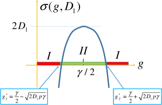
In this section we calculate the contributions to $P(V)$ from the log-normal $P_{{\rm LN}}(V)$ and Gaussian $P_{{\rm Gauss}}(V)$ parts to (17).

One can easily compute the variance of the Gaussian part of $P_{{\rm Gauss}}(V)$ leaving in it only the bi-diagonal terms with $i=i^{\prime}$ and $j=j^{\prime}$:

$$\langle V^{2}\rangle=\int\limits_{g\in II}dg\,N^{-\frac{1}{p\gamma}\left(g-\frac{\gamma}{2}\right)^{2}-2g}$$

$$\sim {\rm max}_{g\in II}\left\{N^{-\frac{1}{p\gamma}\left(g-\frac{\gamma}{2}\right)^{2}-2g}\right\}\equiv N^{-\gamma_{{\rm eff}}}.$$

The maximum in (B) at $g$ belonging to region II in Fig. 8 can be reached (i) inside the region II at $g=g^{*}_{1}$, (ii) at the border of this region at $g=g^{*}_{2}$, and (iii) at the cut-off of $P(g)$ at $g^{*}=0$ (see Fig. 8 and Fig. 9(left)).

Figure 9: (Color online) (a) Different possible positions $g^{*}_{1}$, $g^{*}_{2}$ or $g^{*}=0$ that maximize  (B) in region II depending on $p$, $\gamma$ and $D_{1}$. The reference of maximum realized in each sector of parameters is shown by an ikon in the corresponding sector. (b) Different possible positions $g^{*}_{1}$, $g^{*}_{2}$ or $g^{*}=0$ that maximize  (52) in region I. The reference of maximum realized in each sector of parameters is shown by an ikon in the corresponding sector. For $D_{1}>\gamma/8p$ the maximum in  (52) is reached at the edge of the right segment of region I, $g=g_{2^{\prime}}^{*}$ (not to be confused with the edge of the left segment $g=g_{2}^{*}$, see Fig. 8 ). It leads to a higher branch of the orange curve $\Delta(\alpha)/\gamma+\alpha$ in Fig. 3 (not shown in Fig. 3) which is separated by a gap from the blue curve in Fig. 3 and thus is irrelevant for our analysis.

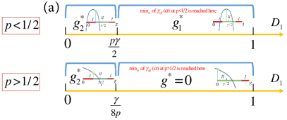
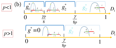
The expression for $\gamma_{{\rm eff}}(D_{1)}$ takes the form:

$$\gamma_{{\rm eff}}(D_{1})=\left\{\begin{array}[]{ll}\gamma(1-p),&\frac{p\gamma}{2}<D_{1}<1,\;p<\frac{1}{2}\cr 2D_{1}+\gamma-2\sqrt{2D_{1}\gamma p},&D_{1}<\min\left(\frac{p\gamma}{2},\frac{\gamma}{8p}\right)\cr\frac{\gamma}{4p},&\frac{\gamma}{8p}<D_{1}<1,\;p\geq\frac{1}{2}\end{array}\right..$$ (51)

Next we compute the function

$$\Delta(D_{1})=-2{\rm max}_{g\in I}\left\{\sigma(g,D_{1})-g-D_{1}\right\}.$$ (52)

in (21).

The details of the calculation which is similar to calculation of $\gamma_{{\rm eff}}(D_{1})$ in (B) are illustrated in Fig. 9(right). The resulting expression for $\Delta(D_{i})$ is:

$$\Delta(D_{1})=\left\{\begin{array}[]{ll}\frac{\gamma}{2}\left(1-\frac{p}{2}\right)-D_{1},&0<D_{1}<\frac{\gamma p}{8},\;p<1\cr D_{1}+\frac{\gamma}{2}-\sqrt{2D_{1}\gamma p},&\frac{\gamma p}{8}<D_{1}<\frac{\gamma}{8p},\;p<1\cr\frac{\gamma}{4p}-D_{1},&0<D_{1}<\frac{\gamma}{8p},\;p\geq 1\end{array}\right..$$ (53)

In the end of this section we consider the question of the distribution of $g_{ij}=-\ln|H_{ij}-H^{\prime}_{ij}|/\ln N$ with log-normal distributed $H=N^{-g_{1}}$ and $H^{\prime}=N^{-g_{2}}$. Applying the usual logarithmic approximation $\ln|H-H^{\prime}|\approx\ln{\rm max}\{|H|,|H^{\prime}|\}$, we approximate

$$g_{ij}=\min(g_{1},g_{2})$$ (54)

and, thus, the distribution $P(g)$ is given by

$$P(g)=P(g_{1}=g)\int\limits_{g}^{\infty}P(g_{2})dg_{2}\simeq\left\{\begin{array}[]{lr}P(g_{1}=g)&g<\gamma/2\\ P^{2}(g_{1}=g)&g>\gamma/2\\ \end{array}\right.$$ (55)

As one can see from Fig. 9 the latter region $g>\gamma/2$ is actual only for the upper branch $g_{2^{\prime}}^{*}$ of $\Delta(D_{1})+D_{1}$ for $D_{1}>\gamma/(8p)$ which never contributes to the phase diagram.

Appendix C Kullback-Leibler measures in the multifractal phase

In this section we give a more detailed quantitative description of ${\rm KL1}$ and ${\rm KL2}$ measures.

We begin by considering the simpler correlation function, ${\rm KL2}$. For that we employ the ansatz for the wavefunction moments:

$$M_{q}=\left\langle\sum_{i}|\psi_{\mu}(i)|^{2q}\right\rangle=N^{-D_{q}(q-1)}\,f_{q}(L/\xi_{q}),$$ (56)

where $D_{q}$ is the fractal dimension in the corresponding phase and $f_{q}(x)$ is the crossover scaling function:

$$f_{q}(L/\xi_{q}\rightarrow\infty)\rightarrow\left\{\begin{array}[]{ll}{\rm const}.&\;\;{\rm multifractal\;\;phase}\cr{\rm const}.\,N^{(q-1)(D_{q}-1)},&\;\;{\rm ergodic\;\;phase}\cr{\rm const}.\,N^{(q-1)D_{q}}&\;\;{\rm localized\;\;phase}\end{array}\right.$$ (57)

that tends to a constant as $L\rightarrow\infty$.

Note that graphs with the local tree structure and for LN-RP matrices the length scale $L\propto\ln N$, so that the scaling function is in general a function of two arguments $\ln N/\xi_{q}$ and $N/e^{\xi_{q}}$ representing the length- and volume scaling García-Mata et al. (2017, 2020). On the finite-dimensional lattices $N\propto L^{d}$, and the volume scaling can be represented as the length scaling in the modified scaling function. In this case a single argument $L/\xi_{q}$ is sufficient.

When $L\propto\ln N$ the volume scaling is the leading one for $L\gg\xi_{q}$, and it is this scaling that provides the asymptotic behavior (57). The length scaling is important in the crossover region $L\lesssim\xi_{q}$. Below for brevity we will use the short-hand notation $L/\xi_{q}$ in all the cases.

There are two trivial cases: $M_{0}=N$ and $M_{1}=1$ (which follows from the normalization of wave function). As a consequence we have $D_{0}=1$ and

$$f_{0}(x)=f_{1}(x)\equiv 1.$$ (58)

Next using the statistical independence of $\psi$ and $\tilde{\psi}$ in (29) and normalization of wave functions we represent

$${\rm KL2}=\left\langle\sum_{i}|\psi(i)|^{2}\,\ln|\psi(i)|^{2}\right\rangle-N^{-1}\left\langle\sum_{i}\ln|\psi(i)|^{2}\right\rangle.$$ (59)

Now we express both terms in (59) in terms of $M_{q}$ using the identity:

$$\ln|\psi_{\alpha}(i)|^{2}=\lim_{\epsilon\rightarrow 0}\epsilon^{-1}\,(|\psi_{\alpha}(i)|^{\epsilon}-1)$$ (60)

The first term is equal to:

$$\left\langle\sum_{i}\lim_{\epsilon\rightarrow\infty}\frac{|\psi(i)|^{2(1+\epsilon)}-|\psi(i)|^{2}}{\epsilon}\right\rangle=\lim_{\epsilon\rightarrow\infty}\left[\frac{1}{\epsilon}\left(M_{1+\epsilon}-1\right)\right].$$ (61)

The second term can be expressed as:

$$-\frac{1}{N}\left\langle\sum_{i}\lim_{\epsilon\rightarrow\infty}\frac{|\psi(i)|^{2\epsilon}-1}{\epsilon}\right\rangle=-\lim_{\epsilon\rightarrow 0}\left[\frac{1}{\epsilon}\left(N^{-1}M_{\epsilon}-1\right)\right].$$ (62)

Now expanding $M_{1+\epsilon}$ and $M_{\epsilon}$ in the vicinity of $q=0,1$ and defining

$$f_{1+\epsilon}(x) = 1+\epsilon\,\varphi_{1}(x)+O(\epsilon^{2});$$ (63)

$$f_{\epsilon}(x) = 1-\epsilon\,\varphi_{0}(x)+O(\epsilon^{2}),$$ (64)

we obtain:

$${\rm KL2}={\rm KL2}_{c}(N)+\varphi_{0}(L/\xi_{0})+\varphi_{1}(L/\xi_{1}),$$ (65)

where ${\rm KL2}_{c}$ is logarithmically divergent, as in (33):

$${\rm KL2}_{c} = \ln N\,(1-\partial_{\epsilon}D_{\epsilon}|_{\epsilon=0}-D_{1})+{\rm const}.$$ (66)

$$= \ln N\,(\alpha_{0}-D_{1})+{\rm const}.$$

Here we used the identity

$$\alpha_{0}=\frac{d\tau_{\epsilon}}{d\epsilon}\left|{}_{\epsilon=0}\right.=\partial_{\epsilon}[D_{\epsilon}(\epsilon-1)]\left|{}_{\epsilon=0}\right..$$ (67)

for $\alpha_{0}$ describing the typical value of the wave function amplitude:

$$|\psi(i)|_{typ}^{2}=N^{-\alpha_{0}}$$ (68)

Note that, generally speaking, the characteristic lengths $\xi_{0}\sim|\gamma-\gamma_{c}|^{-\nu^{(0)}}$ and $\xi_{1}\sim|\gamma-\gamma_{c}|^{-\nu^{(1)}}$ in $\phi_{0}$ and $\phi_{1}$ may have different critical exponents $\nu^{(0)}$ and $\nu^{(1)}$. If this is the case, the smallest one will dominate the finite-size corrections near the critical point:

$${\rm KL2}-{\rm KL2}_{c}(N)=\Phi_{2}(L|\gamma-\gamma_{c}|^{\nu_{2}}),\;\;\;\nu_{2}={\rm min}\{\nu^{(0)},\nu^{(1)}\}.$$ (69)

(69) is employed in this paper for the numerical characterization of the phases by finite size scaling (FSS). One can see from (66) that ${\rm KL2}$ is logarithmically divergent in the multifractal phase, as $\alpha_{0}>1$ and $D_{1}<1$ and the scaling functions $\varphi_{0}(x)$ and $\varphi_{1}(x)$ tend to a finite $N$-independent limit. It is also logarithmically divergent in the localized phase, as in (32), where one can formally set $D_{1}=0$ in (66):

$${\rm KL2}_{c}=\alpha_{0}\,\ln N.$$ (70)

However, in the ergodic phase the logarithmic divergence of ${\rm KL2}$ is gone, since in this case $\alpha_{0}=D_{1}=1$ in (66). One can easily show using the Porter-Thomas distribution:

$$P_{PT}(x=N|\psi(i)|^{2})=\frac{e^{-x/2}}{\sqrt{2\pi\,x}}$$ (71)

that ${\rm KL2}=2$ in the fully-ergodic phase.

At the continuous ergodic transition, where the correlation length $\xi=\infty$ and $\alpha_{0}=D_{1}=1$, the critical value ${\rm KL2}_{c}(N)$ of ${\rm KL2}$ is independent of $N$. This results in crossing at $\gamma=\gamma_{ET}$ of all the curves for ${\rm KL2}$ at different values of $N$ which helps to identify the ergodic transition Pino et al. (2019).

Figure 10: (Color online) The best collapse of the $KL1$ and $KL2$ data for LN-RP with $p=1$ and $p=0.5$. The collapse for $KL1$ and $KL2$ is done in the vicinity of the localization (for $KL1$) and ergodic (for $KL2$) transitions by recursive procedure that finds $\gamma_{c}$ and $\nu$ by minimizing the mean square deviation of data from a smooth scaling function which is updated at any step of the procedure. (insets) The critical value of $KL1$ and $KL2$ as a function of $\ln N$. It stays almost a constant for $KL1$ and for $KL2$ at $p=0.5$ when the ergodic transition is continuous and well separated from the localized one but it grows logarithmically in $N$ at $p=1$ when the ergodic and localization transitions merge together. This growth is the reason of smearing of the intersection of $KL2$ curves in Fig. 4. The exponent $\nu$ significantly depends on $p$ and is consistent with $\nu_{1}\approx\nu_{2}=0.5$ at $p=1$ and $\nu_{2}=1$ at $p=0.5$.

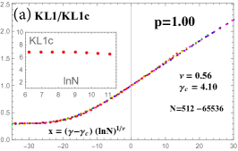
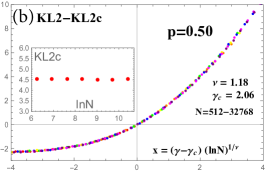
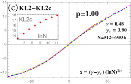
However, if the ergodic transition coincides with the Anderson localization transition and is characterized by a jump in fractal dimension, (i.e. $\alpha_{0}$ and $D_{1}$ are not equal to 1 at the transition), the critical value ${\rm KL2}_{c}(N)$ is no longer $N$-independent. In this case the crossing is smeared out and can disappear whatsoever. Nonetheless, by subtracting ${\rm KL2}_{c}$ from ${\rm KL2}$ one can still locate the transition point from the best collapse of ${\rm KL2}$ vs. $\gamma$ curves by choosing an optimal $\gamma_{c}$ and $\nu_{2}$ in (69). However, it is safer to use ${\rm KL1}$ in this case.

The derivation of finite size scaling (FSS) for ${\rm KL1}$ proceeds in the same way by plugging the identity  (60) into:

$${\rm KL}1=\left\langle\sum_{i}|\psi_{\alpha}(i)|^{2}\,\ln|\psi_{\alpha}(i)|^{2}-\sum_{i}|\psi_{\alpha}|^{2}\,\ln|\psi_{\alpha+1}(i)|^{2}\right\rangle.$$ (72)

and employing the ansatz:

$$\left\langle\sum_{i}|\psi_{E}(i)|^{2q_{1}}\,|\psi_{E+\omega}(i)|^{2q_{2}}\right\rangle\sim N^{1+\beta}\,N_{\omega}^{\alpha}$$

$$\times\,F_{q_{1},q_{2}}(L/\xi_{q_{1}},L/\xi_{q_{2}}),$$ (73)

where $N_{\omega}=1/(\rho\omega)$ and $\rho$ is the mean DoS.

Applying for large $\omega\sim\rho^{-1}$ ($N_{\omega}\simeq 1$) the “decoupling rule”:

$$\left\langle\sum_{i}|\psi_{E}(i)|^{2q_{1}}\,|\psi_{E+\omega}(i)|^{2q_{2}}\right\rangle\sim$$

$$\sum_{i}\left\langle|\psi_{E}(i)|^{2q_{1}}\right\rangle\,\left\langle|\psi_{E+\omega}(i)|^{2q_{2}}\right\rangle,$$ (74)

and for small $\omega\sim\delta$ ($N_{\omega}\simeq N$) the “fusion rule”:

$$\left\langle\sum_{i}|\psi_{E}(i)|^{2q_{1}}\,|\psi_{E+\omega}(i)|^{2q_{2}}\right\rangle\sim\\ \left\langle\sum_{i}|\psi_{E}(i)|^{2q_{1}+2q_{2}}\right\rangle,$$ (75)

one easily finds:

$$\beta = -2+D_{q_{1}}(1-q_{1})+D_{q_{2}}(1-q_{2}),$$ (76)

$$\alpha+\beta = -1+D_{q_{1}+q_{2}}(1-q_{1}-q_{2}).$$

Due to the “fusion rule” for $\psi_{\alpha}$ and $\psi_{\alpha+1}$ we obtain from  (56):

$$\left\langle\sum_{i}|\psi_{\alpha}(i)|^{2q_{1}}\,|\psi_{\alpha+1}(i)|^{2q_{2}}\right\rangle\sim F_{q_{1},q_{2}}(L/\xi_{q_{1}+q_{2}})$$

$$\times N^{-D_{q_{1}+q_{2}}(q_{1}+q_{2}-1)}.$$ (77)

Substituting (C) in (60), (72) we observe cancelation of the leading logarithmic in $N$ terms in ${\rm KL1}$ in the multifractal phase:

$${\rm KL1}_{c}={\rm const}.$$ (78)

We obtain:

$${\rm KL1}=\Phi_{1}(L|\gamma-\gamma_{c}|^{\nu_{1}}).$$ (79)

where $\nu_{1}=\nu^{(1)}\geq\nu_{2}$ and the crossover scaling function $\Phi_{1}(x)$ is:

$$\Phi_{1}(x)=\partial_{\epsilon}f_{1+\epsilon}(x)-\partial_{\epsilon}f_{1,\epsilon}(x)|_{\epsilon=0}.$$ (80)

As it is seen from (79), ${\rm KL1}$ is independent of $N$ at the Anderson transition point $\gamma=\gamma_{AT}$. Thus all curves for ${\rm KL1}$ at different values of $N$ intersect at $\gamma=\gamma_{AT}$. This gives us a powerful instrument to identify the Anderson localization transition point.

Note that the coefficient in front of $\ln N$ in ${\rm KL2}$ may help to detect discontinuity of the Anderson transition. Indeed, one can use the Mirlin-Fyodorov symmetry of fractal dimensions to establish the relation, see (33):

$$\alpha_{0}=2-D_{1},\;\;\;\Rightarrow\alpha_{0}-D_{1}=2(1-D_{1}).$$ (81)

This tells us immediately that for continuous Anderson transition which is characterized by vanishing $D_{1}$ both just below and just above the transition, the coefficient in front of $\ln N$ in ${\rm KL2}$ is equal to $2$. In particular, we conclude that $\alpha_{0}$ on the localized side of the transition is equal to $2$. It appears that in LN-RP this value

$$\alpha_{0}=2,\;\;\;\;(\gamma=\gamma_{AT}+0).$$ (82)

in the localized phase just above the transition remains equal to $2$ in all the cases. This is in contrast to the corresponding coefficient $2(1-D_{1})$ in front of $\ln N$ in ${\rm KL2}$ just below the transition which is smaller than $2$ if there is a jump in the fractal dimension at the transition. Such a jump in the coefficient in front of $\ln N$ in ${\rm KL2}$ is a signature of the discontinuity of the transition which is the most easily detectable numerically, see Fig. 5.

Appendix D Finite-size scaling collapse for $KL1$ and $KL2$.

The next step is to analyze the finite-size scaling (FSS) by a collapse of the data for ${\rm KL1}$ and ${\rm KL2}$ at different $N$ in the vicinity of the localization and ergodic transition, respectively. To this end we use the form of FSS derived in IS C.

$${\rm KL1} =\Phi_{1}(\ln N|\gamma-\gamma_{AT}|^{\nu_{1}}),$$ (83a)

$${\rm KL2}-{\rm KL2_{c}(N)} =\Phi_{2}(\ln N|\gamma-\gamma_{ET}|^{\nu_{2}}).$$ (83b)

The input data for the collapse is ${\rm KL1}$ and ${\rm KL2}$ versus $\gamma$ for $7$ values of $N$ is shown in Fig. 4. The fitting parameters extracted from the best collapse are $\nu_{1}$ ($\nu_{2}$) and the critical points $\gamma_{AT}$ ($\gamma_{ET}$). The critical value of ${\rm KL2}_{c}(N)={\rm KL2}(\gamma_{ET},N)$ is determined by the best fitting for $\gamma_{ET}$. For the localization transition where the critical point $\gamma_{AT}$ is well defined by the intersection in ${\rm KL1}$, one may look for the best collapse by fitting only $\nu_{1}$.

The plots of Fig. 10 demonstrate the quality of the collapse for several representative cases. In the insets of the figures we show the $\ln N$- dependence of the critical values of ${\rm KL1}$, ${\rm KL2}$ which were obtained numerically from ${\rm KL1}(\gamma=\gamma_{AT},N)$ and ${\rm KL2}(\gamma=\gamma_{ET},N)$, respectively, with $\gamma_{AT}$ and $\gamma_{ET}$ found from the best collapse. It is demonstrated that the critical value of ${\rm KL1}$ is almost $N$-independent, as well as the critical value of ${\rm KL2}$ at $p=1/2$ when the continuous ergodic transition is well separated from the Anderson localization one. However, at $p=1$ when ET and AT merge together the critical value of ${\rm KL2}$ increases linearly with $\ln N$, signaling of the critical multifractal state at the Anderson transition point, very similar to the case of 3D Anderson transition. This $\ln N$-dependence of ${\rm KL2}_{c}$ is the reason of smearing out of the intersection point in ${\rm KL2}$ shown in Fig. 4.

Appendix E Ratio of typical and mean LDOS

Figure 11: [upper panels] Plots of the typical $\rho_{{\rm typ}}$ (solid lines) and mean $\rho_{{\rm av}}$ (dashed lines) LDOS and [lower panels] of the second derivative of $\rho_{{\rm typ}}/\rho_{{\rm av}}$ w.r.t. $\eta$ for the log-normal RP model at (left panel) $p=0.01$ in the multifractal phase $\gamma_{ET}<\gamma=1.5<\gamma_{AT}$, (other panels) $p=1.0$ in the weakly ergodic phase $\gamma_{FWE}<\gamma=2.0$, $3.2$, $3.8<\gamma_{ET}=\gamma_{AT}$. The positions of the maxima of the second derivative are shown by crosses of the corresponding color for all system sizes in the range from $N=512$ (dark blue) to $N=16384$ (red). Notice a plateau developing in $\rho_{{\rm typ}}$ for intermediate values of $\eta$ with increasing the system size. The maximum of the second derivative is always inside the plateau region or on its right end. The plateau gradually shrinks with increasing $\gamma$ and disappears in the localized phase.

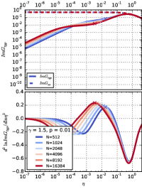
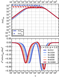
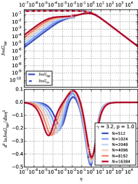
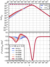
In this section we consider in more details the technical issue with the determination of the order parameter for the FWE transition

$$\phi(\eta)=1-\frac{\rho_{{\rm typ}}}{\rho_{{\rm av}}}\ ,$$ (84)

being the ratio of the typical, $\rho_{{\rm typ}}$, and the mean, $\rho_{{\rm av}}$, LDOS given by the expressions

$$\ln\rho_{{\rm typ}}=\left\langle\ln\rho(x,E+i\eta)\right\rangle,\quad\rho_{{\rm av}}=\left\langle\rho(x,E+i\eta)\right\rangle,$$ (85)

with the LDOS before averaging written as

$$\rho(x,E+i\eta)=\sum_{\mu}|\psi_{\mu}(x)|^{2}\frac{\eta/\pi}{(E-E_{\mu})^{2}+\eta^{2}}\ .$$ (86)

The averaging in (85) is taken over the disorder realizations, over all coordinates $x$ (which are statistically equivalent in LN-RP) and over $100$ energy values in the middle half of the spectrum.

As mentioned in the main text the ratio $\rho_{{\rm typ}}/\rho_{{\rm av}}$ develops the plateau $\sim N^{-1+D_{1}}$ in some range of bare level width parameter $\eta\gg\delta$ large compared to the typical level spacing $\delta$. However, at any finite sizes this plateau has a finite slope, especially for the WE phase where $N^{D_{1}}=fN$ with a $N$-independent constant $f<1$ and, thus, the plateau is also $N$-independent

$$\phi(\eta\gg\delta)\propto 1-f=O(1)\$$ (87)

which is zero in the FE phase, $f=1$, and finite in the WE one, $f<1$.

Figure 12: Plots for $\phi=1-\rho_{{\rm typ}}/\rho_{{\rm av}}$ as a function of $\gamma$ at $p=0.5$, $1$, $2$, $3$ for $N=512$, $1024$, $2048$, $4096$, $8192$ (from blue to red) and extrapolated to $N=\infty$ (black). The gray dashed lines represent cubic polynomial fits to the points of extrapolation away from the transition. The intersection of each of these lines with $\phi=0$ gives the numerical estimate of $\gamma_{{\rm FWE}}$ (shown by bright blue point) which is compared in Table 2 with the predicted by (13) in the main text.

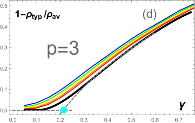
In order to find the FWE transition accurately we develop the procedure of the automatic selection of $\eta$ in the middle of the underdeveloped plateau. For this purpose we take the second derivative of the ratio $\rho_{{\rm typ}}/\rho_{{\rm av}}$ w.r.t. $\eta$ after the smoothening it with the $5$-degree spline and find the point of maximum of this derivative lying in between of two local minima (see the lower panels in Fig. 11). Figure 11 shows several examples for $p=0.01$ and $p=1$ where the positions of the maxima of the second derivative are shown by crosses of the corresponding color for all system sizes $N$.

Appendix F Location of FWE transition

The behavior of the order parameter (84) helps to locate the FWE transition. In Fig. 12 we present the plots for $\phi=1-\rho_{{\rm typ}}/\rho_{{\rm av}}$ for different values of $p$ as a function of $\gamma$ calculated numerically by exact diagonalization for several values of $N$ and then extrapolated to $N=\infty$ as follows. Similarly to the critical exponents $\tau_{q}(N)$ Evers et al. (2001); Luitz et al. (2020) or the spectrum of fractal dimensions $f(\alpha,N)$ De Luca et al. (2014); Kravtsov et al. (2015); Nosov et al. (2019); Nosov and Khaymovich (2019); Deng et al. (2020) we show that a linear in $1/\ln N$ function

$$\phi(\gamma,p,N)=\phi(\gamma,p)+\frac{c(\gamma,p)}{\ln N}$$ (88)

fits the data points at fixed $(\gamma,p)$ for the available range of $N$ and take $\phi(\gamma,p)$ as an extrapolated value.

p	$0.50$	$0.75$	$1.00$	$2.00$	$3.00$
$\gamma_{FWE}^{theor}$	$0.66$	$0.57$	$0.5$	$0.33$	$0.25$
$\gamma_{FWE}^{num}$	$0.67\pm 0.04$	$0.57\pm 0.04$	$0.49\pm 0.04$	$0.28\pm 0.07$	$0.22\pm 0.07$

Table 2: Comparison of analytical predictions (red), (13), and numerical data (blue) for the FWE transition points. Numerical data is obtained by exact diagonalization of LN-RP random matrices with $N=512-8192$ followed by extrapolation to $N\rightarrow\infty$ of the order parameter, (84), given by the ratio of the typical $\rho_{{\rm typ}}$ and the mean $\rho_{{\rm av}}$ local DOS.

Figure 13: (Color online) Plots for ${\rm KL2}$ as a function of $\gamma$ at $p=0.5$ (a) and $2$ (b) for $N=512$, $1024$, $2048$, $4096$, $8192$ (from blue to red) and extrapolated to $N=\infty$ (black). The gray dashed lines represent cubic polynomial fits to the points of extrapolation away from the transition. The intersection of each of these lines with the RMT value ${\rm KL2}=2$ gives the numerical estimate of $\gamma_{{\rm FWE}}$ (shown by bright blue point).

Figure 14: (Color online) Scaling of the spectral bandwidth $E_{BW}$ with $N$ in different regions of $p$: (a) $p=1/2$; (b) $p=1$; (c) $p=1.5$ extracted numerically from the fitting to $E_{BW}=cN^{\beta}$ of the eigenvalue standard deviation $\sigma_{E}=\langle(E-\langle E\rangle)^{2}\rangle^{1/2}$, the averaged absolute deviation of $E$ from its mean $\sigma_{1,E}=\langle|E-\langle E\rangle|\rangle$, the mean $\delta=\langle E_{n+1}-E_{n}\rangle$ and typical $\delta_{typ}=\exp\langle\ln\left(E_{n+1}-E_{n}\right)\rangle$ global level spacings multiplied by $N$ for the system sizes $N=512-32768$. All measures are calculated over the $90$ % of the states in the middle of the spectrum. The dashed lines represent the analytical prediction, Eq. (96), in the ergodic phases, $\gamma<\gamma_{ET}$, while in the non-ergodic ones $E_{BW}=W\sim N^{0}$.

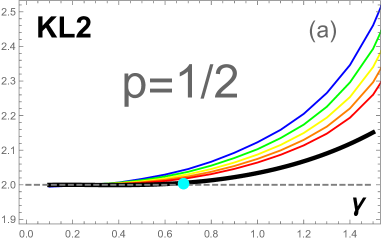
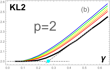
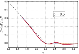
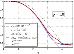
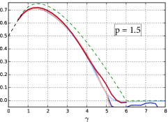
While this extrapolation (shown by black curves in the figures) is reliable away from the transition, it is not able to give the true singularity at the transition which would require an extrapolation from much larger matrix sizes. Therefore for numerical location of the transition $\gamma$ we used the cubic polynomial fit to the points of extrapolation sufficiently remote from the transition (represented by gray dashed lines in Fig.12). Intersection of these lines with the dashed line $\phi=0$ gives the numerical estimate of $\gamma_{{\rm FWE}}$. Almost the same values of $\gamma_{{\rm FWE}}$ can be obtained by studying ${\rm KL2}$ statistics (with the same extrapolation procedure given by Eq. (88)). Some of the plots for ${\rm KL2}$ vs $\gamma$ are presented in Fig.13.

The results of this analysis are summarized and compared with the prediction of Eq.(13) in Table 2. One can see that (13) is well reproduced by our numerics.

Appendix G Mean and typical Breit-Wigner width of the mini-band

According to the definition (7) and the Fermi Golden rule the Breit-Wigner width is given by the following sum

$$\Gamma_{n}\sim\rho_{av}\sum_{m=1\atop|H_{mn}|<E_{BW}}^{N}|H_{mn}|^{2}$$ (89)

where $\rho_{av}\sim 1/E_{BW}$ is the mean global DOS and the spectral bandwidth $E_{BW}=\max(W,\Gamma)$ is given by the maximum of the bare on-site bandwidth $W$ and the mean Breit-Wigner miniband width

$$\Gamma=\langle\Gamma_{n}\rangle\sim\frac{N\langle|H_{mn}|^{2}\rangle_{E_{BW}}}{E_{BW}}$$ (90)

and should be found self-consistently.

The typical Breit-Wigner width

$$\Gamma_{typ}=\exp\langle\ln\Gamma_{n}\rangle\sim S_{3}^{1/2}\sim\frac{N|H_{typ}|^{2}}{E_{BW}}$$ (91)

determines the FWE transition (9).

Let’s first calculate $\Gamma$ for different cases.

In the non-ergodic phases $\Gamma\ll E_{BW}\sim W$ and, thus, it is given by (10) with $q=2$ as

$$\Gamma\sim S_{2}\sim N^{1-\gamma/\gamma_{ET}}\ ,$$ (92)

with $\gamma_{ET}$ given by (12).

In the opposite limit of $\Gamma\gg W$ one should calculate the second moment of $H_{mn}$ self-consistently, taking into account in (90) $E_{BW}\simeq\Gamma$. Parameterizing $\Gamma\sim S_{2}^{1/2}\sim N^{\beta}$ and $|H_{mn}|\sim N^{\alpha}$ with certain parameters $\beta>0$ and $\alpha<\beta$, one obtains self-consistency equation

$$N^{2\beta-1}\sim\int\limits\limits_{-\infty}^{\beta}N^{2\alpha-\frac{(\alpha+\gamma/2)^{2}}{p\gamma}}d\alpha\ ,$$ (93)

where the integral can be calculated in the saddle-point approximation.

For all $\beta>\alpha_{\max}=\gamma\left(p-\frac{1}{2}\right)$ and $\beta>0$ one obtains:

$$\beta=\frac{1}{2}-\frac{\gamma}{2}\left(1-p\right)\ .$$ (94)

The above conditions on $\beta$ restrict the validity range of this formula to $\gamma<\min\left(\frac{1}{p};\frac{1}{1-p}\right)$.

In the opposite limit of $0<\beta<\gamma\left(p-\frac{1}{2}\right)$ the main contribution to the integral in (93) is given by $\alpha=\beta$ leading to

$$2\beta-1=2\beta-\frac{(\beta+\gamma/2)^{2}}{p\gamma}\Leftrightarrow\beta=\sqrt{p\gamma}-\frac{\gamma}{2}\ .$$ (95)

The above conditions on $\beta$ restrict the validity range of the latter to $\frac{1}{p}<\gamma<4p$ which is achievable only for $p>\frac{1}{2}$.

As a result a new crossover parameter $\gamma_{0}=\frac{1}{p}$ emerges in the scaling of $\Gamma$ with $N$:

$$\Gamma\sim\left\{\begin{array}[]{ll}N^{\frac{1-\gamma(1-p)}{2}},&\gamma<\gamma_{ET},\gamma_{0}\\ N^{\sqrt{p\gamma}-\frac{\gamma}{2}},&\gamma_{0}<\gamma<\gamma_{ET}\\ N^{1-\gamma/\gamma_{ET}},&\gamma>\gamma_{ET}\end{array}\right.$$ (96)

For the first two cases (corresponding to the ergodic phases) where $\Gamma$ determines the bandwidth $E_{BW}$ we also check the above results numerically by calculating the scaling of different measures of the total bandwidth, see Fig. 14. In all these cases a semi-quantitative agreement is demonstrated with deviations for $p\geq 1$ caused probably by finite-size effects.

An important result of these numerics is that for $90$ % of the states (excluding $10$ % near the band edges) the typical and the mean measures of $E_{BW}$ scale in the same way.

Now we calculate the typical Breit-Wigner width given by (91) and show that the transition point $\gamma_{FWE}$, (13), is not affected by the presence of the crossover parameter $\gamma_{0}=1/p$. Indeed, from (91) and (96) one obtains

$$\Gamma_{typ}\sim\left\{\begin{array}[]{ll}N^{\frac{1-\gamma(1+p)}{2}},&\gamma<\gamma_{ET},\gamma_{0}\\ N^{1-\sqrt{p\gamma}-\frac{\gamma}{2}},&\gamma_{0}<\gamma<\gamma_{ET}\\ N^{1-\gamma},&\gamma>\gamma_{ET}\end{array}\right.$$ (97)

and it is easy to check that there is the only solution of the equation $\Gamma_{typ}\sim N^{0}$ given by $\gamma=\gamma_{FWE}$.