Nonparametric Feature Impact and Importance

Abstract

Practitioners use feature importance to rank and eliminate weak predictors during model development in an effort to simplify models and improve generality. Unfortunately, they also routinely conflate such feature importance measures with feature impact, the isolated effect of an explanatory variable on the response variable. This can lead to real-world consequences when importance is inappropriately interpreted as impact for business or medical insight purposes. The dominant approach for computing importances is through interrogation of a fitted model, which works well for feature selection, but gives distorted measures of feature impact. The same method applied to the same data set can yield different feature importances, depending on the model, leading us to conclude that impact should be computed directly from the data. While there are nonparametric feature selection algorithms, they typically provide feature rankings, rather than measures of impact or importance. They also typically focus on single-variable associations with the response. In this paper, we give mathematical definitions of feature impact and importance, derived from partial dependence curves, that operate directly on the data. To assess quality, we show that features ranked by these definitions are competitive with existing feature selection techniques using three real data sets for predictive tasks.

1 Introduction

Among data analysis techniques, feature importance is one of the most widely applied and practitioners use it for two key purposes: (1) to select features for predictive models, dropping the least predictive features to simplify and potentially increase the generality of the model and (2) to gain business, medical, or other insights, such as product characteristics valued by customers or treatments contributing to patient recovery. To distinguish the two use cases, we will refer to feature predictiveness for modeling purposes as importance (the usual meaning) and the effect of features on business or medical response variables as impact.

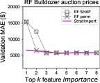
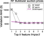
While some feature importance approaches work directly on the data, such as minimal-redundancy-maximal-relevance (mRMR) by Peng et al. (2005), almost all algorithms used in practice rank features by interrogating a fitted model provided by the user. Examples include permutation importance by Breiman (2001), drop column importance, and SHAP by Lundberg and Lee (2017); LIME by Ribeiro et al. (2016) interrogates subsidiary models to analyze such fitted models. It is accepted as self-evident that identifying the most predictive features for a model is best done through interrogation of that model, but this is not always the case. For example, when asked to identify the single most important feature of a real dataset (Kaggle, 2018) for a random forest (RF), the features selected by model-based techniques get twice the validation error of the nonparametric technique proposed in this paper; see Figure 6c. Still, model interrogation is generally very effective in practice for feature importance purposes.

Feature importance should not, however, be interpreted as feature impact for several reasons. First, predictive features do not always coincide with impactful features; e.g., models unable to capture complex nonlinear feature-response relationships rank such features as unimportant, even if they have large impacts on the response. Next, practitioners must develop models accurate enough to yield meaningful feature importances, but there is no definition of “accurate enough.” Finally, it is possible to get very different feature importances (and hence impacts) running the same algorithm on the same data, just by choosing a different model. This is despite the fact that feature impacts are relationships that exist in the data, with or without a model.

Consider the feature importance charts in Figure 1 derived from four different models on the same well-known Boston toy data set, as computed by SHAP. The linear model (a) struggles to capture the relationship between features and response variable (validation $R^{2}$=0.73), so those importances are less trustworthy. In contrast, the (b) RF, (c) boosted trees, and (d) support vector machine (SVM) models capture the relationship well (each with $R^{2}>0.85$). The problem is that SHAP derives meaningfully different feature importances from each model, as most model-based techniques would. The differences arise because feature impact is distorted by the lens’ of the models (yielding importances). The differences might be appropriate for model feature selection, but it is unclear which ranking, if any, gives the feature impacts.

Figure 1: Ranking and relative predictiveness of the top 8 of 13 Boston data set features determined by SHAP interrogating four different models. There is considerable variation between plots even in the two most important features. For example, while RF and XGBoost rank LSTAT and RM first but the RF gives RM much more weight. The SVM reverses that ranking. Model hyperparameters were tuned with 5-fold cross-validation grid search on a variety of hyperparameters over an 80% training set. SHAP explains the 20% validation set.

Unfortunately, practitioners routinely conflate model-based feature importance with impact and have, consequently, likely made business or medical decisions based upon faulty information. Despite the potentially serious real-world consequences resulting from inappropriate application of importances, research attention has focused primarily on feature importance rather than feature impact.

In this paper, we address this deficiency by contributing (1) a straightforward mathematical formula as an ideal for computing feature impact, and related feature importance, that does not require predictions from a fitted model and (2) a prototype implementation called StratImpact that yields plausible feature impacts. By not requiring predictions from a model, we also make feature impact methods accessible to the vast community of business analysts and scientists that lack the expertise to choose, tune, and evaluate models. To assess StratImpact quality, we use importance as a proxy to show that it is competitive on real data with existing importance techniques, as measured by validation errors on models trained using the top $k$ feature importances.

We measure feature impact as a function of its partial dependence curve, as Greenwell et al. (2018) did, because partial dependences (ideally) isolate the effect of a single variable on the response. In contrast to Greenwell et al. (2018), we use a nonparametric method called StratPD (Parr and Wilson 2019) to estimate partial dependences without predictions from a fitted model, which allows us to compute feature impact not just feature importance. StratPD also isolates partial dependence curves in the presence of strong codependencies between features. The partial dependence approach is flexible in that it opens up the possibility of computing importances using any partial dependence method, such as Friedman’s original definition (Friedman 2000) and ALE (Apley and Zhu to appear). (We will refer to Friedman’s original definition as FPD to distinguish it from the general notion of partial dependence.) SHAP also fits into this perspective since the average SHAP value at any single feature value forms a point on a mean-centered partial dependence curve. Our prototype is currently limited to regression but accepts numerical and label-encoded categorical explanatory variables; a similar approach should work for classification. The software is available via Python package stratx with source at github.com/parrt/stratx.

We begin by giving definitions of feature impact and importance in Section 2, then survey existing nonparametric and model-dependent techniques in Section 3. Section 4 assesses the quality of StratImpact importance values by examining how well they rank model features in terms of predictiveness. We finish in Section 5 with a discussion of the proposed technique’s effectiveness and future work.

2 Definitions of impact and importance

In special circumstances, we know the precise impact of each feature $x_{j}$. Assume we are given the training data pair ($\bf X,y$) where ${\bf X}=[x^{(1)},\ldots,x^{(n)}]$ is an $n\times p$ matrix whose $p$ columns represent observed features and ${\bf y}$ is the $n\times 1$ vector of responses; ${\bf X}_{j}$ is the $n\times 1$ column of data associated with feature $x_{j}$. If a data set is generated using a linear function, $y=\beta_{0}+\sum_{j=1}^{p}\beta_{j}x_{j}$, then coefficient $\beta_{j}$ corresponds to the impact of $x_{j}$ for $j=1,..,p$. $\beta_{j}$ is the impact on $y$ for a unit change in feature $x_{j}$, holding other features constant.

To hold features constant for any smooth and continuous generator function $f:\mathbb{R}^{p}\rightarrow\mathbb{R}$ that precisely maps each $x^{(i)}$ to $y^{(i)}$, ${y^{(i)}}=f(x^{(i)})$, we can take the partial derivatives of $f$ with respect to each feature $x_{j}$; e.g., for linear functions, ${\partial y}/{\partial x_{j}}=\beta_{j}$. Integrating the partial derivative then gives the idealized partial dependence (Parr and Wilson 2019) of $y$ on $x_{j}$, the isolated contribution of $x_{j}$ at $z$ to $y$:

$$\text{\it PD}_{j}(x_{j}=z)=\int_{min(x_{j})}^{z}\frac{\partial f}{\partial x_{j}}dx_{j}$$ (1)

Using partial derivatives to isolate the effect of variables on the response was used prior to StratPD by ALE (Apley and Zhu to appear) and Integrated Gradients (IG) (Sundararajan et al. 2017). The key distinction is that StratPD integrates over the derivative of the generator function, ${\partial f}/{\partial x_{j}}$, estimated from the raw training data, whereas, previous techniques integrate over the derivative of model $\hat{f}$ that estimates $f$: ${\partial\hat{f}}/{\partial x_{j}}$. While there are advantages to using models, such as their ability to smooth over noise, properly choosing and tuning a machine learning model presents a barrier to many user communities, such as business analysts, scientists, and medical researchers. Further, without potential distortions from a model, StratPD supports the measurement of impact, not just importance.

2.1 Impact and importance for numerical features

To go from the idealized partial dependence of $x_{j}$ to feature impact, we assume that the larger the “mass” under $x_{j}$’s partial dependence curve, the larger $x_{j}$’s impact on $y$.

Definition 1 The (non-normalized) nonparametric feature impact of $x_{j}$ is the area under the magnitude of $x_{j}$’s idealized partial dependence:

$$\textsc{Impact}_{j}=\int_{\min({\bf X}_{j})}^{\max({\bf X}_{j})}|PD_{j}(x_{j})|dx_{j}$$ (2)

In practice, we approximate the integral with a Riemann sum of rectangular regions:

$$\textsc{Impact}_{j}\approx\sum_{x_{j}\in\{{\bf X}_{j}\}}|PD_{j}(x_{j})|\Delta x_{j}$$ (3)

where $\{{\bf X}_{j}\}$ is the set of unique ${\bf X}_{j}$ values ($\{{\bf X}_{j}^{(i)}\}_{i=1..n}$) and $n_{j}$ is the number of unique ${\bf X}_{j}$. The usual definition of region width, $\Delta x_{j}={(\max({\bf X}_{j})-\min({\bf X}_{j}))}/{n_{j}}$, is inappropriate in practice because ${\bf X}_{j}$ often has large gaps in $x_{j}$ space and impact units would include $x_{j}$’s units (e.g., $rent\times bedrooms$ or $rent\times hasparking$). That would make impact scores incomparable across features. By defining $\Delta x_{j}=1/n_{j}$, the fraction of unique ${\bf X}_{j}$ values covered by one $PD_{j}$ value, widths are not skewed by empty $x_{j}$ gaps and impact units become those of $y$. That reduces $x_{j}$’s impact estimate to the average magnitude of $PD_{j}$:

This formula works for any partial dependence curve, either by examining output from a fitted model, $\hat{f}$, or by estimating the partial derivative of $f$ directly from the data and then integrating, as StratPD does. Dividing $x_{j}$’s impact by the sum of all impacts, converts impact units from $y$’s units to [0,1]:

$$\textsc{Impact}_{j}\approx\sum_{x_{j}\in\{{\bf X}_{j}\}}|PD_{j}(x_{j})|\times\frac{1}{n_{j}}=\overline{|PD_{j}|}$$

Definition 2 The normalized nonparametric feature impact of $x_{j}$ is the ratio of the average magnitude of $x_{j}$’s partial dependence to the total for all variables:

$$\textsc{Impact}_{j}^{*}=\frac{\overline{|\text{\it PD}_{j}|}}{\sum_{k=1}^{p}\overline{|\text{\it PD}_{k}|}}$$ (4)

Intuitively, the impact of $x_{j}$ is how much, on average, the values of $x_{j}$ are expected to push $y$ away from a zero baseline. We deliberately chose this definition instead of measuring how much $x_{j}$ pushes $y$ away from the average response, $\overline{y}$, as SHAP does. The average response includes the effects of all $x_{j}$, which hinders isolation of individual feature impacts. For example, the impact of $x_{1}$ on quadratic $y=x_{1}^{2}+x_{2}+100$ is $x_{1}^{2}$, not $|\overline{y}-x_{1}^{2}|$.

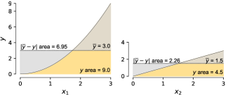
Figure 2 illustrates how the area under the $x_{1}^{2}$ and $x_{2}$ PD curves differ from the area straddling the means for $x_{1},x_{2}\sim U(0,3)$. The area under-the-curve ratio of $x_{1}$-to-$x_{2}$ is 2-to-1 (9/4.5), whereas the ratio of the area straddling the mean has roughly a 3-to-1 ratio (6.95/2.26). The symbolic partial derivatives are ${\partial y}/{\partial x_{1}}=2x_{1}$ and ${\partial y}/{\partial x_{2}}=1$, so $\text{\it PD}_{1}=x_{1}^{2}$ and $\text{\it PD}_{2}=x_{2}$. Integrating those gives $\textsc{Impact}_{1}=\int_{0}^{3}x_{1}^{2}dx_{1}=\frac{x_{1}^{3}}{3}\big{|}_{0}^{3}=9$ and $\textsc{Impact}_{2}=\int_{0}^{3}x_{2}^{2}dx_{2}=\frac{x_{2}^{2}}{2}\big{|}_{0}^{3}=4.5$; $\textsc{Impact}_{1}^{*}=0.\overline{66}$ and $\textsc{Impact}_{2}^{*}=0.\overline{33}$.

Figure 2: The area under $x_{1}$ and $x_{2}$ PD curves represent $\textsc{\small StratImpact}_{1}$, $\textsc{\small StratImpact}_{2}$ for $y=x_{1}^{2}+x_{2}+100$ in range $[0,3]$. Compare the areas straddling the means and the areas under the partial dependence curves.

Figure 3: StratImpact curve for bulldozer SalePrice on YearMade including the histogram used to weight the partial dependence to obtain feature importances. A 20k sample of all 363k records; ~0.5% of samples stratified into regions with single YearMade values.

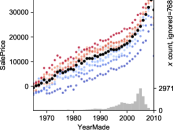
The $PD_{j}$ curve represents how $x_{j}$ effects $y$, but does not take into consideration the distribution of $x_{j}$ in ${\bf X}_{j}$. Consider the StratPD curve and $x_{j}$ histogram in Figure 3 for feature YearMade from the bulldozer auction data set (Kaggle, 2018). The colored curves represent ten bootstraps from the same training set and the black dots give the average curve. From a business perspective, knowing that increases in bulldozer age continue to reduce price is useful, but new bulldozers will represent the bulk of any model validation set. Because model feature selection is often assessed using validation error, feature selection is sensitive to the distribution of $x_{j}$. This suggests that feature importance should take into consideration the distribution of $x_{j}$, leading to the following importance definition:

Definition 3 The normalized nonparametric feature importance of $x_{j}$ is the ratio of $x_{j}$’s average partial dependence magnitude, weighted by $x_{j}$’s distribution, to the total of all weighted averages:

$$\textsc{Import}_{j}^{*}=\frac{\textsc{Import}_{j}}{\sum_{k=1}^{p}\textsc{Import}_{k}}$$ (5)

where

$$\textsc{Import}_{j}\approx\sum_{x_{j}\in\{{\bf X}_{j}\}}\frac{n_{x_{j}}}{n}\times|PD_{j}(x_{j})|$$ (6)

and $n_{x_{j}}$ is the number of $x_{j}$ values in ${\bf X}_{j}$; i.e., $(x_{j},n_{x_{j}})_{x_{j}\in\{{\bf X}_{j}\}}$ is the histogram of ${\bf X}_{j}$.

Measuring impact as the average partial dependence generalizes to non-ordinal categorical explanatory features encoded as unique integers, with a small modification.

2.2 Impact and importance for categorical features

Partial dependence curves for numerical features use the leftmost $x_{j}$ value as the zero reference point, but nominal categorical features have no meaningful order. That implies we can choose any category as the zero reference category, which shifts the partial dependence plot up or down, but does not alter the relative $y$ values among the category levels. For example, consider relative $y$ values for four categories (0, 1, 1, 1) where the first category is the reference. Choosing the second category as the reference yields relative $y$ values (-1, 0, 0, 0). The impacts (average magnitude) for these two variations are 3/4 versus 1/4, respectively, but the choice of reference category should not affect the impact metric computed on the same partial dependence data. Worse, picking a category level whose $y$ is an outlier strongly biases the impact because the outlier pushes up (or down) all category $y$ values by a biased amount. Instead of picking a specific level as the reference, therefore, we use that feature’s partial dependence average value as the reference zero:

Definition 4 The normalized nonparametric categorical feature impact of $x_{j}$ is the ratio of the average magnitude of $x_{j}$’s mean-centered partial dependence to the total for all variables:

$$\textsc{CatImpact}_{j}^{*}=\frac{\overline{|\text{\it PD}_{j}-\overline{\text{\it PD}_{j}}|}}{\sum_{k=1}^{p}\overline{|\text{\it PD}_{k}-\overline{\text{\it PD}_{j}}|}}$$ (7)

The definition of categorical variable importance mirrors the definition for numerical variables, which weights impact by the distribution of the $x_{j}$’s:

Definition 5 The normalized nonparametric categorical feature importance of $x_{j}$ is the ratio of $x_{j}$’s expected mean-centered partial dependence magnitude to the total of all:

$$\textsc{CatImport}_{j}^{*}=\frac{\textsc{CatImport}_{j}}{\sum_{k=1}^{p}\textsc{CatImport}_{k}}$$ (8)

where

$$\textsc{CatImport}_{j}\approx\sum_{x_{j}\in\{{\bf X}_{j}\}}\frac{n_{x_{j}}}{n}\times|PD_{j}(x_{j})-\overline{\text{\it PD}_{j}}|$$ (9)

By choosing $\overline{\text{\it PD}_{j}}$ as the reference value (instead of a specific category’s $\text{\it PD}_{j}$ value), our definition moves closer to SHAP’s mean-centered approach, which we disagreed with above, but only out of necessity for categorical variables. A key difference is that $\textsc{CatImport}_{j}$ centers on $\overline{\text{\it PD}_{j}}$ rather than the overall average, $\bar{y}$, that includes the effect of all features. With these definitions in mind, we make a more detailed comparison to related work in the next section.

3 Existing methods

In this paper, we are primarily concerned with identifying the most impactful features, such as needed in business or medical applications. But, because virtually all related research focuses on feature importance and, because practitioners commonly assume feature importance is the same as feature impact, it is appropriate to compare StratImpact to feature importance methods. Feature importance methods for labeled data sets (with both $\bf X$ and $\bf y$) are broadly categorized into data analysis and model analysis techniques, sometimes called filter and wrapper methods (Tsanas et al., 2010). Data analysis techniques analyze the data directly to identify important features, whereas model analysis techniques rely on predictions from fitted models.

3.1 Data analysis techniques

The simplest technique to identify important or relevant regression features is to rank them by their Spearman’s rank correlation coefficient (Spearman, 1904); the feature with the largest coefficient is taken to be the most important. This method works well for independent features, but suffers in the presence of codependent features. Groups of features with similar relationships to the response variable receive the same or similar ranks, even though just one should be considered important.

Another possibility is to use principle component analysis (PCA), which operates on just the $\bf X$ explanatory matrix. PCA transforms data into a new space characterized by eigenvectors of $\bf X$ and identifies features that explain the most variance in the new space. If the first principal component covers a large percentage of the variance, the “loads” associated with that component can indicate importance of features in the original $\bf X$ space. PCA is limited to linear relationships, however, and “most variation” is not always the same thing as “most important.”

For classification data sets, the Relief algorithm (Kira and Rendell, 1992) tries to identify features that distinguish between classes through repeated sampling of the data. For a sampled observation $x^{(i)}$, the algorithm finds the nearest observation with the same class (hit) and the nearest observation with the other class (miss). The score of each attribute, $x_{j}$, is then updated according to the distance from the selected $x^{(i)}$ to the hit and miss observations’ $x_{j}$ values. ReliefF (Kononenko et al., 1997) extended Relief to work on multiclass problems and RReliefF (Robnik-Sikonja and Kononenko, 1997) adapted the technique to regression problems by “…introduc[ing] a kind of probability that the predicted values of two instances are different.”

In an effort to deal with codependencies, data analysis techniques can rank features not just by relevance (correlation with the response variable) but also by low redundancy, the amount of information shared between codependent features, which is the idea behind minimal-redundancy-maximal-relevance (mRMR) by Peng et al. (2005). mRMR selects features in order according to the following score.

$$J_{\text{mRMR}}(x_{k})=I(x_{k},y)-\frac{1}{|S|}\sum_{x_{j}\in S}I(x_{k},x_{j})$$

where $I(x_{k},x_{j})$ is some measure of mutual information between $x_{k}$ and $x_{j}$, $S$ is the growing set of selected features, and $x_{k}$ is the candidate feature. mRMR only considers single-feature relationships with the response variable, and is limited to classification. See Zhao et al. (2019) for a recent application of mRMR at Uber Technologies. For more on model-free feature importances, see the survey by Li et al. (2017). Tsanas et al. (2010) suggests using Spearman’s rank and not mutual information. Meyer et al. (2008) looks for pairs of features to response variable associations as an improvement, while retaining reasonable efficiency. See Bommert et al. (2020) for benchmarks comparing data analysis methods.

The fundamental problem faced by these data analysis techniques is that they measure relevance by the strength of the association between (typically) a single feature to response $y$, but $y$ contains the impact of all $x_{j}$ variables. Some analysis techniques, such as mRMR, only rank features and do not provide a numerical feature impact. Computing an appropriate association metric between categorical and numerical values also presents a challenge.

3.2 Model-based techniques

Turning to model-based techniques, feature importance methods are typically variations on one of two themes: (1) tweaking a model and measuring the tweak’s effect on model prediction accuracy or expected model output or (2) examining the parameters of a fitted model. The simplest approach following the first theme is drop-column importance, which defines $x_{j}$ importance as the difference in some accuracy metric between a model with all features (the baseline) and a model with $x_{j}$ removed. The model must be retrained $p$ times and highly-correlated features yield low or zero importances because codependent features cover for the dropped column.

To avoid retraining the model, $x_{j}$ can be permuted instead of dropped for permutation importance (Breiman 2001). This approach is faster but can introduce nonsensical observations by permuting invalid values into records, as discussed in Hooker and Mentch (2019); e.g., shifting a true pregnant value into a male’s record. Codependent features tend to share importance, at least when permutation importance is applied to RF models. To avoid nonsensical records for the RF case, Strobl et al. (2008) proposed a conditional permutation importance using the feature space partition created by node splitting during tree construction.

Rather than removing or permuting entire columns of data, LIME (Ribeiro et al., 2016) focuses on model behavior at the observation level. For an observation of interest, $\bf x$, LIME trains an interpretable linear model, on a small neighborhood of data around $\bf x$ to explain the relationship between variables and the response locally. SHAP was shown to subsume the LIME technique in Lundberg and Lee (2017).

SHAP has its roots in Shapley regression values (Lipovetsky and Conklin, 2001) where (linear) models were trained on all possible subsets of features. Let $\hat{f}_{S}$ be the model trained on feature subset $x_{S}$ for $S\subset F=\{1,2,..,p\}$. Each possible model pair differing in a single feature $x_{j}$ contributes the difference in model pair output towards the Shapley value for $x_{j}$. The complete Shapley value is the average model-pair difference weighted by the number of possible pairs differing in just $x_{j}$:

$$\phi_{j}(\hat{f},x_{F})=\sum_{S\subseteq F\texttt{\char 92\relax}\{j\}}\ \frac{|S|!(|F|-|S|-1)!}{|F|!}\ (\hat{f}_{S\cup\{j\}}(x_{S\cup\{j\}})-\hat{f}_{S}(x_{S}))$$ (10)

The SHAP importance for feature $x_{j}$ is the average magnitude of all $\phi_{j}$ values.

To avoid training a combinatorial explosion of models with the various feature subsets, SHAP approximates $\hat{f}_{S}(x_{S})$, with $\operatorname{\mathbb{E}}[\hat{f}(x_{S},{\bf X}_{\texttt{\char 92\relax}S}^{\prime})|{\bf X}_{S}^{\prime}=x_{S}]$ where ${\bf X^{\prime}}$ is called the background set (in “interventional” mode) and users can pass in, for example, a single vector with ${\bf X}_{\texttt{\char 92\relax}S}$ column averages or even the entire training set, ${\bf X}_{\texttt{\char 92\relax}S}$. SHAP’s implementation further approximates $\operatorname{\mathbb{E}}[\hat{f}(x_{S},{\bf X}_{\texttt{\char 92\relax}S}^{\prime})|{\bf X}_{S}^{\prime}=x_{S}]$ with $\operatorname{\mathbb{E}}[\hat{f}(x_{S},{\bf X}_{\texttt{\char 92\relax}S}^{\prime})]$, which assumes feature independence and allows extrapolation of $\hat{f}$ to nonsensical records like permutation importance. By removing the expectation condition, the inner difference of equation (10) reduces to a function of FPDs, which means SHAP can have biased results in the presence of codependent features, as shown in Parr and Wilson (2019). As implemented, then, the average SHAP value at any $x_{j}$ value is a point on the $FPD_{j}-\bar{y}$ curve and so $\overline{|FPD_{j}-\bar{y}|}$ = $\overline{|\phi_{j}(\hat{f},x)|}$.

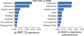
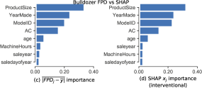
That observation begs the question of whether measuring the area under a simple mean-centered FPD curve would be just as effective as the current SHAP implementation. Figure 4 compares feature importances derived from FPD curves and SHAP values for two real data sets, rent from Kaggle (2017) and bulldozer from Kaggle (2018). The rank and magnitude of the feature importances are very similar between the techniques for the top $p=8$ features. At least for these examples, the complex machinery of SHAP is unnecessary because nearly the same answer is available using a simple FPD.

Figure 4: Importance ranking of top 8 features for rent and bulldozer data sets demonstrating strong similarity between average magnitude of Friedman’s partial dependence curves, (a) and (c), and average magnitude of SHAP values, (b) and (d). 20,000/5,000 training/validation records were sampled to tune an RF model by 5-fold cross validation grid search. Rent validation $R^{2}=0.857$, bulldozer $R^{2}=0.856$. The FPD curve and SHAP values were computed using 300 records from the validation set; SHAP used 100 backing records from the training data.

There are two methods used heavily in practice that define importance in terms of model parameters. The first operates on linear models and divides $\beta$ coefficients by their standard errors and the second examines the decision nodes in tree-based methods. The most well-known tree-based method is “mean drop in impurity” (also called “gini drop”) by Breiman et al. (1984), but there are a number of variations, such as the technique for gradient boosting machines (GBMs) described by Friedman (2000). The importance of $x_{j}$ is the average drop in $y$ impurity, entropy (classification) or variance (regression), for all nodes testing $x_{j}$, weighted by the fraction of test samples that reach those nodes. Such importance measures are known to be biased towards continuous or high cardinality explanatory variables (see Strobl et al. 2007 and Zhou and Hooker 2019).

Deriving feature importances from partial dependences as StratImpact does was previously proposed by Greenwell et al. (2018), and is implemented in an R package called vip, but they defined $x_{j}$’s importance as ${\it PD}_{j}$’s “flatness” rather than the area under the ideal ${\it PD}_{j}$ curve, as we have in equation (1). To measure flatness, they suggest standard deviation for numerical variables and category level range divided by four for categorical variables (as an estimate of standard deviation). Because standard deviation measures the average squared-difference from the average response, vip would likely be more sensitive to partial dependence curve spikes than the area under the curve. Using the idealized partial dependence, vip would measure importance as $\overline{(PD_{j}-\overline{PD_{j}})^{2}}$ akin to SHAP’s mass-straddling-the-mean approach, whereas we suggest the average magnitude weighted by $x_{j}$’s distribution. Another difference between vip and StratImpact is that vip computes partial dependence curves by measuring changes in model $\hat{f}$, rather than directly from the data as we do. Any technique that computes partial dependence curves, directly or indirectly, fits neatly into vip or the “area under the PD curve” framework described in this paper. FPD, ALE, SHAP, and StratPD are four such techniques.

Sundararajan et al. (2017) introduced a technique called integrated gradients (IG) for deep learning classifiers that can also be seen as a kind of partial dependence. To attribute a classifier prediction to the elements of an input vector, $\bf x$, IG integrates over the gradient of the model output function at points along the straight-line path from a baseline vector, $\bf x^{\prime}$, to $\bf x$. IG estimates the integral by averaging the gradient computed at $m$ points and multiplying by the difference between ${\bf x}^{\prime}_{j}$ and ${\bf x}_{j}$:

$$\text{IntegratedGradient}_{j}(\hat{f},{\bf x},{\bf x^{\prime}})=(x_{j}-x^{\prime}_{j})\times\frac{1}{m}\sum_{k=1}^{m}\frac{\partial\hat{f}({\bf x}^{\prime}+\frac{k}{m}({\bf x}-{\bf x}^{\prime}))}{\partial x_{j}}$$ (11)

Because IG integrates the partial derivative like ALE and StratPD, equation (11) can be interpreted as the $x_{j}$ partial dependence curve evaluated at $\bf x$ weighted by the range in $x_{j}$ space. Alternatively, the average gradient within an $x_{j}$ range times the range of $x_{j}$ is equivalent to the area under the $x_{j}$ gradient curve in that range (by the mean value theorem for integrals). In that sense, Sundararajan et al. (2017) is also similar to StratImpact, except that we integrate the gradient twice, once to get the partial dependence curve and a second time to get the area under the partial dependence curve.

StratImpact is neither a model-based technique nor a model-free technique. It does not use model predictions but does rely on StratPD, which internally uses a decision tree model to stratify feature space. StratImpact, therefore, has a lot in common with the “mean drop in impurity” technique. The differences are that users do not provide a fitted tree-based model to StratImpact and StratImpact examines leaf observations rather than decision nodes. Unlike techniques relying on model predictions, StratImpact can compute feature impact rather than feature importance. Unlike model-free techniques (such as mRMR), StratImpact is able to provide impacts not just feature rankings and can consider the relationship between multiple features and the response. StratImpact (via StratPD) also performs well in the presence of codependent variables, unlike many model-based techniques. In the next section, we demonstrate that StratImpact is effective and efficient enough for practical use.

4 Experimental results

Assessing the quality of feature impact and importance is challenging because, even with domain expertise, humans are unreliable estimators (which is why we need data analysis algorithms in the first place). The simplest approach is to examine impacts and importances computed from synthetic data for which the answers are known. For real data sets, we can train a predictive model on the most impactful or most important $k$ features, as identified by the methods of interests, and then compare model prediction errors; we will refer to this as top-$k$. (Peng et al. 2005 and Tsanas et al. 2010 also used this approach.) The method that accurately identifies the most impactful features without getting confused by codependent features should yield lower prediction errors for a given $k$.

In this section, we present the results of several experiments using the toy Boston data set and three real data sets: NYC rent prices (Kaggle, 2017), bulldozer auction sales (Kaggle, 2018), and flight delays (Kaggle, 2015). Rent has $p=20$ features, bulldozer has 14, and flight has 17. We draw $n$=25,000 samples from each data set population, except for Boston which only has 506 records, and split into 80% training / 20% validation sets. Each point on an error curve represents the validation set mean absolute error (MAE) for a given model, feature ranking, and data set. All models used to rank features or measure top-$k$ errors were tuned with 5-fold cross-validation grid search across a variety of hyperparameters using just the training records. (Tuned hyperparameters can be found at the start of file genfigs/support.py in the repo.) The same StratPD and CatStratPD hyperparameters were used across all simulations and datasets.

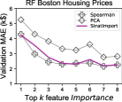
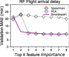
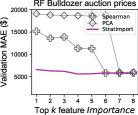
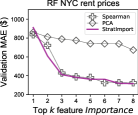
We begin with a baseline comparison of Import to principal component analysis’ (PCA) ranking (“loads” associated with the first component) and to Spearman’s R coefficients computed between each $x_{j}$ and the response variable $y$. Figure 5 shows the MAE curve for an RF model trained using the top-$k$ features as ranked by PCA, Spearman, and Import. Spearman’s R does a good job for all but the bulldozer data set, while PCA performs poorly on all four data sets. Import is competitive with or surpasses these baseline techniques.

(a)

(b)

(c)

(d)

Figure 5: RF MAE curves from baseline rankings computed using RF models trained on Boston, flight, bulldozer, and rent data sets. Error curves represent 5-fold cross validation using the top-$k$ features as ranked by Spearman’s R, PCA “loads” associated with the first component, and Import.

Next, in Figure 6, we compare Import’s rankings to those of ordinary least squares (OLS), RF-based permutation importance, and SHAP interrogating OLS and RF models. A feature’s OLS ranking score is its $\beta$ coefficient divided by its standard error. (OLS is not very useful for the bulldozer data set because there are important label-encoded categorical explanatory variables.) OLS and OLS SHAP analyzed all $n$ records for each data set, but RF-based permutation importance and RF-based SHAP trained on 80% then used the remaining 20% validation set to rank features. We deliberately restricted StratImpact to analyzing just the 80% training data, to see how it would fare. RF-based SHAP and permutation importance, therefore, have two clear advantages: (1) they use the same kind of model (RF) for both feature ranking and for computing top-$k$ error curves and (2) they are able to select features using 100% of the data, but StratImpact selects features using just the training data.

The error curves for StratImpact, RF SHAP, and permutation importance are roughly the same for Boston in Figure 6a and flight in Figure 6b. For bulldozer in Figure 6c, StratImpact’s error curve suggests it selected a more predictive feature than RF SHAP or RF permutation importance for $k=1$: ModelID followed by high-cardinality categorical YearMade. RF permutation importance chose ProductSize as most important followed by ModelID and RF SHAP chose ProductSize followed by YearMade. For the rent data set in Figure 6d, StratImpact selects brooklynheights (L1 distance from the apartment to that neighborhood) as the most predictive feature followed by bedrooms. RF SHAP and permutation importance selected bedrooms followed by bathrooms. The StratImpact curve is very similar to the RF permutation curve. The second row in Figure 6 shows that the plain impact, unweighted by $x_{j}$’s distribution, can also work well for model feature selection purposes. The impact error curves match the importance error curves closely, indicating that $x_{j}$ density is not critical for these data sets.

(a)

(b)

(c)

(d)

Figure 6: RF MAE curves from importance rankings on top and impact rankings on bottom. The mean absolute error curves from 40-tree RF models trained on boston, flight, bulldozer, and rent data sets. Error curves represent 5-fold cross validation using the top-$k$ features from the following feature rankings: OLS as in Figure 5, SHAP interrogating OLS, SHAP interrogating 40-tree RF, permutation importance interrogating 40-tree RF, and StratImpact. All methods had access to 80% training data from $n=25,000$ random sample (Boston has just 506 records). All methods except StratImpact had access to the 20% validation set.

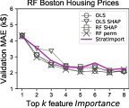
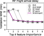
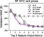
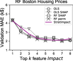
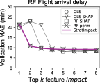
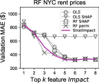
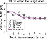
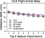
The OLS-derived feature rankings present an interesting story here (the circular markers). For Boston, flight, and rent, OLS feature rankings give error curves that are fairly similar to those of RF SHAP and RF permutation importance. Please keep in mind that, while the features were chosen by interrogating a linear model, the error curves were computed using predictions from a (stronger) RF model. Perhaps most surprising is that OLS chooses the best single most-predictive feature for both flight and rent data sets, choosing TAXI_OUT and bathrooms, respectively; RF SHAP and RF permutation rank DEPARTURE_TIME and bedrooms as most predictive. The circle markers representing OLS in Figure 6b and Figure 6d have the lowest $k=1$ error curve value, suggesting that, for example, the number of bathrooms is more predictive of rent price than bedrooms in New York. The error curve derived from the OLS SHAP feature rankings differs from the OLS curve because the OLS coefficients are divided by the standard error. An error curve using raw OLS coefficients is the same as OLS SHAP’s curve.

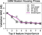
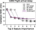
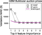
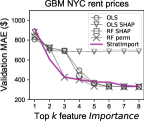
Features that are predictive in one model are not necessarily predictive in another model. To determine how well the feature rankings from the various methods “export” to another model, we trained gradient boosting machines (GBM) on the OLS-based, RF-based, and StratImpact feature rankings. Figure 7 shows that the StratImpact error curves generated using GBM models are similar to those resulting from RF models, except for the Figure 7(b) flight delay curve, which does not improve much after feature $k=5$, while the other feature rankings do improve.

(a)

(b)

(c)

(d)

Figure 7: MAE curves as in Figure 6 except measuring xgboost predictions, rather than RF; hyperparameters were tuned via 5-fold cross validation.

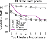
To check feature exportation to a very different model, we computed error curves for the Boston, flight, and rent data sets using OLS regressors, as shown in Figure 8, again using the StratImpact, OLS-derived, and RF-derived rankings. The error curves derived from OLS model predictions are all higher than those from RFs, as expected since OLS is weaker than GBM, but feature rankings from all technique export reasonably well, with the exception of StratImpact’s rankings for rent. The poor performance could be due to OLS’ inability to leverage the StratImpact ranking or could be poor feature ranking on StratImpact’s part. The former is more likely, given that more sophisticated methods get low error curves using StratImpact’s ranking.

Figure 8: MAE curves as in Figure 7 but measuring OLS rather than RF predictions.

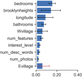
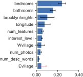
To compute the StratImpact feature rankings described thus far, we used a single 80/20 training and validation sample in order to get reproducible figures. But, different subsets of the data set can yield very different impacts, depending on the variability of the data set. StratImpact supports multiple trials via bootstrapping or subsampling on the $(\bf X,y)$ data set to obtain impact and importance standard deviations. As an example, Figure 8 shows the feature rankings of Impact and Import, averaged from 30 trials using 75% subsamples selected randomly from the complete (cleaned) 49,352 records of the rent data set. The error bars show two standard deviations above and below the average (a red error bar indicates it reaches 0 and was sifted to the bottom). The high variances of the neighborhood features, such as brooklynheights and Evillage, arise because many distance-to-neighborhood features have similar impacts; selection will depend on vagaries of the subsample.

(a) StratImpact Rent Importance

(b) StratImpact Rent Impact

Figure 8: Average feature importance and impact across 30 trials on the rent data set, with 75% subsamples from 49,352 total records. Error bars show two standard deviations. Red indicates two standard deviations reach zero.

Performance is important for practitioners so it is worthwhile analyzing StratImpact time complexity and demonstrating that it operates in a reasonable amount of time. The cost of computing each $x_{j}$’s impact is dominated by the cost of computing the partial dependence but includes a pass over the $x_{j}$ values to compute the mean. Computing the importance costs an extra pass through the data to get a histogram. The upper bound complexity for both StratPD and CatStratPD partial dependences is $O(n^{2})$ in the worst case, which is similar to FPD’s $O(nm)$ for $n$ records and $m$ curve evaluation points. In practice, StratPD typically performs linearly while CatStratPD exhibits mildly quadratic behavior. The overall worst case behavior for StratImpact is then $O(pn^{2})$ to get $p$ impacts and importances. For comparison purposes, ALE is the most efficient at $O(n)$ per feature and SHAP has the hardest time with efficiency due to the combinatorial problem of feature subsetting. SHAP has model-type-dependent optimizations for linear regression, deep learning, and decision-tree based models, but other models are prohibitively expensive. For example, SHAP applied to a support vector machine trained on the 80% Boston training set takes four minutes to explain the 101 records in the 20% validation set.

dataset	$p$	catvars	$n$=1,000	10,000	20,000	30,000	time versus $n$	$R^{2}$
flight	17	6	5.7s	8.9s	35.5s	76.0s	$-0.360n+0.095n^{2}$	0.9945
bulldozer	14	3	0.8s	3.0s	11.4s	24.6s	$-0.063n+0.029n^{2}$	0.9961
rent	20	0	0.4s	4.0s	8.5s	12.9s	$0.424n+0.000n^{2}$	0.9995

Table 1: Execution time for subsets of size 1,000 to 30,000 for rent, bulldozer, flight data sets. There are a total of 40 numerical and 9 categorical variables: rent, bulldozer, and flight have $p=20$, $p=14$, and $p=17$. Rent has no categorical variables and exhibits linear performance, whereas categorical variables introduce mildly quadratic behavior. Final two columns describe how data fits to quadratic equations. Time does not include Numba just-in-time compiler warm-up, but users do experience this warm-up time.

Table 1 summarizes the empirical time in seconds to compute importances for a range of subset sizes for the three Kaggle data sets. The “time versus $n$” and $R^{2}$ columns describe a quadratic fit to the curve representing the time (in seconds) required to compute subsets from $n=1$ to 30,000 stepping by 1,000. The rent data set has no categorical variables and grows linearly with $n$. The flight data set, on the other hand, shows quadratic behavior due to the (six) categorical variables. Despite the worst-case complexity, Table 1 suggests our Python-only StratImpact prototype is fast enough for use on real data sets of sizes in the tens of thousands. When the cost of training and tuning a model is counted, StratImpact would likely outperform other techniques.

Each of the $p$ feature impact computations is independent and could proceed in parallel. Unfortunately, our casual attempts at parallelizing the algorithm across multiple CPU cores was thwarted by Python’s dreaded “global interpreter lock” (threading) or passing data-passing costs between processes (process-based threading). We did, however, get increased performance using the Numba just-in-time compiler (http://numba.pydata.org) on algorithm hotspots (at the cost of 5 seconds of compiler warmup time at runtime).

5 Discussion and future work

In this paper, we propose a nonparametric approach to measuring numerical and categorical feature $x_{j}$’s impact upon the response variable, $y$, based upon a mathematical definition of impact: the area under $x_{j}$’s ideal $PD_{j}$ curve (numerical) or mean-centered $PD_{j}$ curve (categorical). By weighting $x_{j}$’s partial dependence curve with $x_{j}$’s distribution, we arrive at a mathematical definition of feature importance. Our goal is not to claim that existing feature selection techniques are incorrect or fail in practice; they very often work well. Instead, we hope to:

1. Bring attention to the fact that feature importance is not the same as feature impact, because of potential distortions from peering through model $\hat{f}$. The same importance algorithm applied to the same data can get meaningfully different answers from different fitted models. For the purpose of gaining insights into the behavior of objects under consideration (such as customers or patients) or the impact of their features, the ideal impact metric would avoid $\hat{f}$ predictions and operate directly on the data.

2. Demonstrate it is possible to compute impacts without relying on predictions from a fitted model, by estimating partial derivatives of the unknown generator function $f$. This approach is valuable because there are large prospective industrial and scientific communities that lack the expertise to choose and tune machine learning models. Model-free importance techniques do exist, but they usually provide just a ranking, rather than meaningful impact values, and often consider associations of the response with just one or two features at a time.

To assess the quality of StratImpact’s feature impacts, we compared StratImpact’s recommended feature importance rankings to those of other techniques as a proxy. Despite not having access to predictions from a fitted model nor access to the entire data set, StratImpact feature rankings are competitive with other rankings from other commonly-used techniques on Boston and three real data sets. Figure 6c illustrates a case in which StratImpact’s most important feature choice yields half the error rate of the top features recommended by the other methods. One would expect model-based techniques to easily identify the single most important model feature, or at least to do so more readily than an approach not using model predictions. Even if such results are rare, misidentifying this top feature indicates that there is room for improvement in the feature importance research area.

An interesting and unanticipated result is that simple expedient approaches, such as ranking features by Spearman’s R coefficient or permutation importance, perform well at least for the first eight important features in our experiments. (We did not perform experiments on the least important features.) Also, the error curves for SHAP and permutation importance generally mirror each other for the first eight features. Both techniques introduce potentially nonsensical records to avoid retraining models, but this does not appear to affect their ability to rank features for feature selection purposes.

Our proposed approach relies on accurate partial dependences, and considerable effort has gone into refining the StratPD and CatStratPD partial dependence algorithms currently used by StratImpact. Any improvement in the accuracy of estimation techniques for partial dependence curves would be useful in their own right and particularly helpful for StratImpact. The current prototype is limited to regression and so, next, we hope to develop suitable model-free partial dependence and impact algorithms for classification.

References

- Apley and Zhu (to appear) Apley DW, Zhu J (to appear) Visualizing the effects of predictor variables in black box supervised learning models. Journal of the Royal Statistical Society, Series B (Statistical Methodology)
- Bommert et al. (2020) Bommert A, Sun X, Bischl B, RahnenfÃŒhrer J, Lang M (2020) Benchmark for filter methods for feature selection in high-dimensional classification data. Computational Statistics and Data Analysis 143:106839, DOI https://doi.org/10.1016/j.csda.2019.106839, URL http://www.sciencedirect.com/science/article/pii/S016794731930194X
- Breiman (2001) Breiman L (2001) Random forests. Machine Learning 45(1):5–32, DOI 10.1023/A:1010933404324, URL https://doi.org/10.1023/A:1010933404324
- Breiman et al. (1984) Breiman L, Friedman JH, Olshen RA, Stone CJ (1984) Classification and Regression Trees. Wadsworth
- Friedman (2000) Friedman JH (2000) Greedy function approximation: A gradient boosting machine. Annals of Statistics 29:1189–1232
- Greenwell et al. (2018) Greenwell BM, Boehmke BC, McCarthy AJ (2018) A simple and effective model-based variable importance measure. 1805.04755
- Hooker and Mentch (2019) Hooker G, Mentch L (2019) Please stop permuting features: An explanation and alternatives. 1905.03151
- Kaggle (2015) Kaggle (2015) 2015 flight delays and cancellations. https://www.kaggle.com/usdot/flight-delays, accessed: 2019-12-01
- Kaggle (2017) Kaggle (2017) Two sigma connect: Rental listing inquiries. https://www.kaggle.com/c/two-sigma-connect-rental-listing-inquiries, accessed: 2019-06-15
- Kaggle (2018) Kaggle (2018) Blue book for bulldozer. https://www.kaggle.com/sureshsubramaniam/blue-book-for-bulldozer-kaggle-competition, accessed: 2019-06-15
- Kira and Rendell (1992) Kira K, Rendell LA (1992) The feature selection problem: Traditional methods and a new algorithm. In: Proceedings of the Tenth National Conference on Artificial Intelligence, AAAI Press, AAAI 1992, pp 129–134
- Kononenko et al. (1997) Kononenko I, Simec E, Robnik-Sikonja M (1997) Overcoming the myopia of inductive learning algorithms with RELIEFF. Applied Intelligence 7:39–55
- Li et al. (2017) Li J, Cheng K, Wang S, Morstatter F, Trevino RP, Tang J, Liu H (2017) Feature selection. ACM Computing Surveys 50(6):1–45, DOI 10.1145/3136625, URL http://dx.doi.org/10.1145/3136625
- Lipovetsky and Conklin (2001) Lipovetsky S, Conklin M (2001) Analysis of regression in game theory approach. Applied Stochastic Models in Business and Industry 17:319 – 330, DOI 10.1002/asmb.446
- Lundberg and Lee (2017) Lundberg SM, Lee SI (2017) A unified approach to interpreting model predictions. In: Guyon I, Luxburg UV, Bengio S, Wallach H, Fergus R, Vishwanathan S, Garnett R (eds) Advances in Neural Information Processing Systems 30, Curran Associates, Inc., pp 4765–4774, URL http://papers.nips.cc/paper/7062-a-unified-approach-to-interpreting-model-predictions.pdf
- Meyer et al. (2008) Meyer P, Schretter C, Bontempi G (2008) Information-theoretic feature selection in microarray data using variable complementarity. Selected Topics in Signal Processing, IEEE Journal of 2:261 – 274, DOI 10.1109/JSTSP.2008.923858
- Parr and Wilson (2019) Parr T, Wilson JD (2019) Tech report: Partial dependence through stratification. preprint arXiv:190706698 Submitted for peer review
- Peng et al. (2005) Peng H, Long F, Ding C (2005) Feature selection based on mutual information: Criteria of max-dependency, max-relevance, and min-redundancy. IEEE transactions on pattern analysis and machine intelligence 27:1226–38, DOI 10.1109/TPAMI.2005.159
- Ribeiro et al. (2016) Ribeiro MT, Singh S, Guestrin C (2016) Why should I trust you?: Explaining the predictions of any classifier. In: Proceedings of the 22nd ACM SIGKDD international conference on knowledge discovery and data mining, ACM, pp 1135–1144
- Robnik-Sikonja and Kononenko (1997) Robnik-Sikonja M, Kononenko I (1997) An adaptation of relief for attribute estimation in regression. DOI 10.1.1.34.8381, URL https://citeseerx.ist.psu.edu/viewdoc/summary?doi=10.1.1.34.8381
- Spearman (1904) Spearman C (1904) The proof and measurement of association between two things. The American Journal of Psychology 15(1):72–101, URL http://www.jstor.org/stable/1412159
- Strobl et al. (2007) Strobl C, Boulesteix AL, Zeileis A, Hothorn T (2007) Bias in random forest variable importance measures: Illustrations, sources and a solution. BMC Bioinformatics 8(1):25, DOI 10.1186/1471-2105-8-25, URL https://doi.org/10.1186/1471-2105-8-25
- Strobl et al. (2008) Strobl C, Boulesteix AL, Kneib T, Augustin T, Zeileis A (2008) Conditional variable importance for random forests. BMC Bioinformatics 9(1):307, DOI 10.1186/1471-2105-9-307, URL https://doi.org/10.1186/1471-2105-9-307
- Sundararajan et al. (2017) Sundararajan M, Taly A, Yan Q (2017) Axiomatic attribution for deep networks. In: Proceedings of the 34th International Conference on Machine Learning - Volume 70, JMLR.org, ICML’17, p 3319–3328
- Tsanas et al. (2010) Tsanas A, Little MA, McSharry PE (2010) A simple filter benchmark for feature selection. URL https://www.semanticscholar.org/paper/A-Simple-Filter-Benchmark-for-Feature-Selection-Tsanas-Little/d9d8acd669caa089731ef3475f03f186f75c518d
- Zhao et al. (2019) Zhao Z, Anand R, Wang M (2019) Maximum relevance and minimum redundancy feature selection methods for a marketing machine learning platform. 1908.05376
- Zhou and Hooker (2019) Zhou Z, Hooker G (2019) Unbiased measurement of feature importance in tree-based methods. 1903.05179