The Heavy-Tail Phenomenon in SGD

Abstract

In recent years, various notions of capacity and complexity have been proposed for characterizing the generalization properties of stochastic gradient descent (SGD) in deep learning. Some of the popular notions that correlate well with the performance on unseen data are (i) the ‘flatness’ of the local minimum found by SGD, which is related to the eigenvalues of the Hessian, (ii) the ratio of the stepsize $\eta$ to the batch-size $b$, which essentially controls the magnitude of the stochastic gradient noise, and (iii) the ‘tail-index’, which measures the heaviness of the tails of the network weights at convergence. In this paper, we argue that these three seemingly unrelated perspectives for generalization are deeply linked to each other. We claim that depending on the structure of the Hessian of the loss at the minimum, and the choices of the algorithm parameters $\eta$ and $b$, the distribution of the SGD iterates will converge to a heavy-tailed stationary distribution. We rigorously prove this claim in the setting of quadratic optimization: we show that even in a simple linear regression problem with independent and identically distributed data whose distribution has finite moments of all order, the iterates can be heavy-tailed with infinite variance. We further characterize the behavior of the tails with respect to algorithm parameters, the dimension, and the curvature. We then translate our results into insights about the behavior of SGD in deep learning. We support our theory with experiments conducted on synthetic data, fully connected, and convolutional neural networks.

1 Introduction

The learning problem in neural networks can be expressed as an instance of the well-known population risk minimization problem in statistics, given as follows:

$$\min\nolimits_{x\in\mathbb{R}^{d}}F(x):=\mathbb{E}_{z\sim\mathcal{D}}[f(x,z)],$$ (1.1)

where $z\in\mathbb{R}^{p}$ denotes a random data point, $\mathcal{D}$ is a probability distribution on $\mathbb{R}^{p}$ that denotes the law of the data points, $x\in\mathbb{R}^{d}$ denotes the parameters of the neural network to be optimized, and $f:\mathbb{R}^{d}\times\mathbb{R}^{p}\mapsto\mathbb{R}_{+}$ denotes a measurable cost function, which is often non-convex in $x$. While this problem cannot be attacked directly since $\mathcal{D}$ is typically unknown, if we have access to a training dataset $S=\{z_{1},\dots,z_{n}\}$ with $n$ independent and identically distributed (i.i.d.) observations, i.e., $z_{i}\sim_{\text{i.i.d.}}\mathcal{D}$ for $i=1,\dots,n$, we can use the empirical risk minimization strategy, which aims at solving the following optimization problem (Shalev-Shwartz and Ben-David, 2014):

$$\min_{x\in\mathbb{R}^{d}}f(x):=f(x,S):=(1/n)\sum\nolimits_{i=1}^{n}f^{(i)}(x),$$ (1.2)

where $f^{(i)}$ denotes the cost induced by the data point $z_{i}$. The stochastic gradient descent (SGD) algorithm has been one of the most popular algorithms for addressing this problem:

$$x_{k}=x_{k-1}-\eta\nabla\tilde{f}_{k}(x_{k-1}),$$ (1.3)

$$\text{ where }\>\>\>\>\nabla\tilde{f}_{k}(x):=(1/b)\sum\nolimits_{i\in\Omega_{k}}\nabla f^{(i)}(x).$$

Here, $k$ denotes the iterations, $\eta>0$ is the stepsize (also called the learning-rate), $\nabla\tilde{f}$ is the stochastic gradient, $b$ is the batch-size, and $\Omega_{k}\subset\{1,\dots,n\}$ is a random subset with $|\Omega_{k}|=b$ for all $k$.

Even though the practical success of SGD has been proven in many domains, the theory for its generalization properties is still in an early phase. Among others, one peculiar property of SGD that has not been theoretically well-grounded is that, depending on the choice of $\eta$ and $b$, the algorithm can exhibit significantly different behaviors in terms of the performance on unseen test data.

A common perspective over this phenomenon is based on the ‘flat minima’ argument that dates back to Hochreiter and Schmidhuber (1997), and associates the performance with the ‘sharpness’ or ‘flatness’ of the minimizers found by SGD, where these notions are often characterized by the magnitude of the eigenvalues of the Hessian, larger values corresponding to sharper local minima (Keskar et al., 2017). Recently, Jastrzębski et al. (2017) focused on this phenomenon as well and empirically illustrated that the performance of SGD on unseen test data is mainly determined by the stepsize $\eta$ and the batch-size $b$, i.e., larger $\eta/b$ yields better generalization. Revisiting the flat-minima argument, they concluded that the ratio $\eta/b$ determines the flatness of the minima found by SGD; hence the difference in generalization. In the same context, Şimşekli et al. (2019b) focused on the statistical properties of the gradient noise $(\nabla\tilde{f}_{k}(x)-\nabla f(x))$ and illustrated that under an isotropic model, the gradient noise exhibits a heavy-tailed behavior, which was also confirmed in follow-up studies (Zhang et al., 2020; Zhou et al., 2020). Based on this observation and a metastability argument (Pavlyukevich, 2007), they showed that SGD will ‘prefer’ wider basins under the heavy-tailed noise assumption, without an explicit mention of the cause of the heavy-tailed behavior. More recently, Xie et al. (2021) studied SGD with anisotropic noise and showed with a density diffusion theory approach that it favors flat minima.

In another recent study, Martin and Mahoney (2019) introduced a new approach for investigating the generalization properties of deep neural networks by invoking results from heavy-tailed random matrix theory. They empirically showed that the eigenvalues of the weight matrices in different layers exhibit a heavy-tailed behavior, which is an indication that the weight matrices themselves exhibit heavy tails as well (Ben Arous and Guionnet, 2008). Accordingly, they fitted a power law distribution to the empirical spectral density of individual layers and illustrated that heavier-tailed weight matrices indicate better generalization. Very recently, Şimşekli et al. (2020) formalized this argument in a mathematically rigorous framework and showed that such a heavy-tailed behavior diminishes the ‘effective dimension’ of the problem, which in turn results in improved generalization. While these studies form an important initial step towards establishing the connection between heavy tails and generalization, the originating cause of the observed heavy-tailed behavior is yet to be understood.

Contributions. In this paper, we argue that these three seemingly unrelated perspectives for generalization are deeply linked to each other. We claim that, depending on the choice of the algorithm parameters $\eta$ and $b$, the dimension $d$, and the curvature of $f$ (to be precised in Section 3), SGD exhibits a ‘heavy-tail phenomenon’, meaning that the law of the iterates converges to a heavy-tailed distribution. We rigorously prove that, this phenomenon is not specific to deep learning and in fact it can be observed even in surprisingly simple settings: we show that when $f$ is chosen as a simple quadratic function and the data points are i.i.d. from a continuous distribution supported on $\mathbb{R}^{d}$ with light tails, the distribution of the iterates can still converge to a heavy-tailed distribution with arbitrarily heavy tails, hence with infinite variance. If in addition, the input data is isotropic Gaussian, we are able to provide a sharp characterization of the tails where we show that (i) the tails become monotonically heavier for increasing curvature, increasing $\eta$, or decreasing $b$, hence relating the heavy-tails to the ratio $\eta/b$ and the curvature, (ii) the law of the iterates converges exponentially fast towards the stationary distribution in the Wasserstein metric, (iii) there exists a higher-order moment (e.g., variance) of the iterates that diverges at most polynomially-fast, depending on the heaviness of the tails at stationarity. More generally, if the input data is not Gaussian, our monotonicity results extend where we can show that a lower bound on the thickness of the tails (which will be defined formally in Section 3) is monotonic with respect to $\eta,b,d$ and the curvature. To the best of our knowledge, these results are the first of their kind to rigorously characterize the empirically observed heavy-tailed behavior of SGD with respect to the parameters $\eta$, $b$, $d$, and the curvature, with explicit convergence rates. Finally, we support our theory with experiments conducted on both synthetic data and neural networks. Our experimental results provide strong empirical support that our theory extends to deep learning settings for both fully connected and convolutional networks.

2 Technical Background

Heavy-tailed distributions with a power-law decay. A real-valued random variable $X$ is said to be heavy-tailed if the right tail or the left tail of the distribution decays slower than any exponential distribution. We say $X$ has heavy (right) tail if $\lim_{x\rightarrow\infty}\mathbb{P}(X\geq x)e^{cx}=\infty$ for any $c>0$. Similarly, an $\mathbb{R}^{d}$-valued random vector $X$ has heavy tail if $u^{T}X$ has heavy right tail for some vector $u\in\mathbb{S}^{d-1}$, where $\mathbb{S}^{d-1}:=\{u\in\mathbb{R}^{d}:\|u\|=1\}$ is the unit sphere in $\mathbb{R}^{d}$.

Heavy tail distributions include $\alpha$-stable distributions, Pareto distribution, log-normal distribution and the Weilbull distribution. One important class of the heavy-tailed distributions is the distributions with power-law decay, which is the focus of our paper. That is, $\mathbb{P}(X\geq x)\sim c_{0}x^{-\alpha}$ as $x\rightarrow\infty$ for some $c_{0}>0$ and $\alpha>0$, where $\alpha>0$ is known as the tail-index, which determines the tail thickness of the distribution. Similarly, we say that the random vector $X$ has power-law decay with tail-index $\alpha$ if for some $u\in\mathbb{S}^{d-1}$, we have $\mathbb{P}(u^{T}X\geq x)\sim c_{0}x^{-\alpha}$, for some $c_{0},\alpha>0$.

Stable distributions. The class of $\alpha$-stable distributions are an important subclass of heavy-tailed distributions with a power-law decay, which appears as the limiting distribution of the generalized CLT for a sum of i.i.d. random variables with infinite variance (Lévy, 1937). A random variable $X$ follows a symmetric $\alpha$-stable distribution denoted as $X\sim\mathcal{S}\alpha\mathcal{S}(\sigma)$ if its characteristic function takes the form:

$$\mathbb{E}\left[e^{itX}\right]=\exp\left(-\sigma^{\alpha}|t|^{\alpha}\right),\qquad t\in\mathbb{R},$$

where $\sigma>0$ is the scale parameter that measures the spread of $X$ around $0$, and $\alpha\in(0,2]$ is known as the tail-index, and $\mathcal{S}\alpha\mathcal{S}$ becomes heavier-tailed as $\alpha$ gets smaller. The probability density function of a symmetric $\alpha$-stable distribution, $\alpha\in(0,2]$, does not yield closed-form expression in general except for a few special cases. When $\alpha=1$ and $\alpha=2$, $\mathcal{S}\alpha\mathcal{S}$ reduces to the Cauchy and the Gaussian distributions, respectively. When $0<\alpha<2$, $\alpha$-stable distributions have their moments being finite only up to the order $\alpha$ in the sense that $\mathbb{E}[|X|^{p}]<\infty$ if and only if $p<\alpha$, which implies infinite variance.

Wasserstein metric. For any $p\geq 1$, define $\mathcal{P}_{p}(\mathbb{R}^{d})$ as the space consisting of all the Borel probability measures $\nu$ on $\mathbb{R}^{d}$ with the finite $p$-th moment (based on the Euclidean norm). For any two Borel probability measures $\nu_{1},\nu_{2}\in\mathcal{P}_{p}(\mathbb{R}^{d})$, we define the standard $p$-Wasserstein metric (Villani, 2009):

$$\mathcal{W}_{p}(\nu_{1},\nu_{2}):=\left(\inf\mathbb{E}\left[\|Z_{1}-Z_{2}\|^{p}\right]\right)^{1/p},$$

where the infimum is taken over all joint distributions of the random variables $Z_{1},Z_{2}$ with marginal distributions $\nu_{1},\nu_{2}$.

3 Setup and Main Theoretical Results

We first observe that SGD (1.3) is an iterated random recursion of the form $x_{k}=\Psi(x_{k-1},\Omega_{k})$, where the map $\Psi:\mathbb{R}^{d}\times\mathcal{S}\to\mathbb{R}^{d}$, $\mathcal{S}$ denotes the set of all subsets of $\{1,2,\dots,N\}$ and $\Omega_{k}$ is random and i.i.d. If we write $\Psi_{\Omega}(x)=\Psi(x,\Omega)$ for notational convenience where $\Omega$ has the same distribution as $\Omega_{k}$, then $\Psi_{\Omega}$ is a random map and

$$x_{k}=\Psi_{\Omega_{k}}(x_{k-1}).$$ (3.1)

Such random recursions are studied in the literature. If this map is Lipschitz on average, i.e.

$$\mathbb{E}[L_{\Omega}]<\infty,\,\mbox{with}\,L_{\Omega}:=\sup\nolimits_{x,y\in\mathbb{R}^{d}}\frac{\|\Psi_{\Omega}(x)-\Psi_{\Omega}(y)\|}{\|x-y\|},$$ (3.2)

and is mean-contractive, i.e. if $\mathbb{E}\log(L_{\Omega})<0$ then it can be shown under further technical assumptions that the distribution of the iterates converges to a unique stationary distribution $x_{\infty}$ geometrically fast (the Prokhorov distance is proportional to $\rho^{k}$ for some $\rho<1$) although the rate of convergence $\rho$ is not explicitly known in general (Diaconis and Freedman, 1999). However, much less is known about the tail behavior of the limiting distribution $x_{\infty}$ except when the map $\Psi_{\Omega}(x)$ has a linear growth for large $x$. The following result characterizes the tail-index under such assumptions for dimension $d=1$. We refer the readers to Mirek (2011) for general $d$.

Theorem 1

(Mirek (2011), see also Buraczewski et al. (2016)) Assume stationary solution to (3.1) exists and:

(i) There exists a random matrix $M(\Omega)$ and a random variable $B(\Omega)>0$ such that for a.e. $\Omega$, $|\Psi_{\Omega}(x)-M(\Omega)x|\leq B(\Omega)$ for every $x$;

(ii) The conditional law of $\log|M(\Omega)|$ given $M(\Omega)\neq 0$ is non-arithmetic;

(iii) There exists $\alpha>0$ such that $\mathbb{E}|M(\Omega)|^{\alpha}=1$, $\mathbb{E}|B(\Omega)|^{\alpha}<\infty$ and $\mathbb{E}[|M(\Omega)|^{\alpha}\log^{+}|M(\Omega)|]<\infty$ where $\log^{+}(x):=\max(\log(x),0)$.

Then, it holds that $\lim_{t\to\infty}t^{\alpha}\mathbb{P}(|x_{\infty}|>t)=c_{0}$ for some constant $c_{0}>0$.

Relaxations of the assumptions of Theorem 1 which require only lower and upper bounds on the growth of $\Psi_{\Omega}$ have also been recently developed (Hodgkinson and Mahoney, 2020; Alsmeyer, 2016). Unfortunately, it is highly non-trivial to verify such assumptions in practice, and furthermore, the literature does not provide any rigorous connections between the tail-index $\alpha$ and the choice of the stepsize, batch-size in SGD or the curvature of the objective at hand which is key to relate the tail-index to the generalization properties of SGD.

Before stating our theoretical results in detail, let us informally motivate our main method of analysis. Suppose the initial SGD iterate $x_{0}$ is in the domain of attraction of a local minimum $x_{\star}$ of $f$ which is smooth and well-approximated by a quadratic function in this basin. Under this assumption, by considering a first-order Taylor approximation of $\nabla f^{(i)}(x)$ around $x_{\star}$, we have

$$\nabla f^{(i)}(x)\approx\nabla f^{(i)}(x_{\star})+\nabla^{2}f^{(i)}(x_{\star})(x-x_{\star}).$$

By using this approximation, we can approximate the SGD recursion (1.3) as:

$$x_{k} \approx x_{k-1}-(\eta/b)\sum\nolimits_{i\in\Omega_{k}}\nabla^{2}f^{(i)}(x_{\star})x_{k-1}$$

$$\quad+(\eta/b)\sum\nolimits_{i\in\Omega_{k}}\left(\nabla^{2}f^{(i)}(x_{\star})x_{\star}-\nabla f^{(i)}(x_{\star})\right)$$

$$=:\left(I-(\eta/b)H_{k}\right)x_{k-1}+q_{k},$$ (3.3)

where $I$ denotes the identity matrix of appropriate size. Here, our main observation is that the SGD recursion can be approximated by an affine stochastic recursion. In this case, the map $\Psi_{\Omega}(x)$ is affine in $x$, and in addition to Theorem 1, we have access to the tools from Lyapunov stability theory Srikant and Ying (2019) and implicit renewal theory for investigating its statistical properties (Kesten, 1973; Goldie, 1991). In particular, Srikant and Ying (2019) study affine stochastic recursions subject to Markovian noise with a Lyapunov approach and show that the lower-order moments of the iterates can be made small as a function of the stepsize while they can be upper-bounded by the moments of a Gaussian random variable. In addition, they provide some examples where higher-order moments are infinite in steady-state. In the renewal theoretic approach, the object of interest would be the matrix $(I-\frac{\eta}{b}H_{k})$ which determines the behavior of $x_{k}$: depending on the moments of this matrix, $x_{k}$ can have heavy or light tails, or might even diverge.

In this study, we focus on the tail behavior of the SGD dynamics by analyzing it through the lens of implicit renewal theory. As, the recursion (3.3) is obtained by a quadratic approximation of the component functions $f^{(i)}$, which arises naturally in linear regression, we will consider a simplified setting and study it in great depth this dynamics in the case of linear regression. As opposed to prior work, this formalization will enable us to derive sharp characterizations of the tail-index and its dependency to the parameters $\eta,b$ and the curvature as well as rate of convergence $\rho$ to the stationary distribution. Our analysis technique lays the first steps for the analysis of more general objectives, and our experiments provide strong empirical support that our theory extends to deep learning settings.

We now focus on the case when $f$ is a quadratic, which arises in linear regression:

$$\min\nolimits_{x\in\mathbb{R}^{d}}F(x):=(1/2)\mathbb{E}_{{(a,y)}\sim\mathcal{D}}\left[\left(a^{T}x-y\right)^{2}\right]\,,$$ (3.4)

where the data $(a,y)$ comes from an unknown distribution $\mathcal{D}$ with support $\mathbb{R}^{d}\times\mathbb{R}$. Assume we have access to i.i.d. samples $(a_{i},y_{i})$ from the distribution $\mathcal{D}$ where $\nabla f^{(i)}(x)=a_{i}(a_{i}^{T}x-y_{i})$ is an unbiased estimator of the true gradient $\nabla F(x)$. The curvature, i.e. the value of second partial derivatives, of this objective around a minimum is determined by the Hessian matrix $\mathbb{E}(aa^{T})$ which depends on the distribution of $a$. In this setting, SGD with batch-size $b$ leads to the iterations

$$x_{k}=M_{k}x_{k-1}+q_{k}\text{ with}\,\,M_{k}:=I-(\eta/b)H_{k},$$ (3.5)

$$H_{k}:=\sum\nolimits_{i\in\Omega_{k}}a_{i}a_{i}^{T},\,q_{k}:=(\eta/b)\sum\nolimits_{i\in\Omega_{k}}a_{i}y_{i}\,,$$

where $\Omega_{k}:=\{b(k-1)+1,b(k-1)+2,\dots,bk\}$ with $|\Omega_{k}|=b$. Here, for simplicity, we assume that we are in the one-pass regime (also called the streaming setting (Frostig et al., 2015; Jain et al., 2017; Gao et al., 2021)) where each sample is used only once without being recycled. Our purpose in this paper is to show that heavy tails can arise in SGD even in simple settings such as when the input data $a_{i}$ is Gaussian, without the necessity to have a heavy-tailed input data. Consequently, we make the following assumptions on the data throughout the paper:

• $a_{i}$’s are i.i.d. with a continuous distribution supported on $\mathbb{R}^{d}$ with all the moments finite. All the moments of $a_{i}$ are finite.

• $y_{i}$ are i.i.d. with a continuous density whose support is $\mathbb{R}$ with all the moments finite.

We assume (A1) and (A2) throughout the paper, and they are satisfied in a large variety of cases, for instance when $a_{i}$ and $y_{i}$ are normally distributed. Let us introduce

$$h(s):=\lim\nolimits_{k\to\infty}\left(\mathbb{E}\|M_{k}M_{k-1}\dots M_{1}\|^{s}\right)^{1/k}\,,$$ (3.6)

which arises in stochastic matrix recursions (see e.g. Buraczewski et al. (2014)) where $\|\cdot\|$ denotes the matrix 2-norm (i.e. largest singular value of a matrix). Since $\mathbb{E}\|M_{k}\|^{s}<\infty$ for all $k$ and $s>0$, we have $h(s)<\infty$. Let us also define $\Pi_{k}:=M_{k}M_{k-1}\dots M_{1}$ and

$$\rho:=\lim\nolimits_{k\to\infty}(2k)^{-1}\log\left(\mbox{largest eigenvalue of }\Pi_{k}^{T}\Pi_{k}\right)\,.$$ (3.7)

The latter quantity is called the top Lyapunov exponent of the stochastic recursion (3.5). Furthermore, if $\rho$ exists and is negative, it can be shown that a stationary distribution of the recursion (3.5) exists.

Note that by Assumption (A1), the matrices $M_{k}=I-\frac{\eta}{b}H_{k}$ are i.i.d. and by Assumption (A3), the Hessian matrix of the objective (3.4) satisfies $\mathbb{E}(aa^{T})=\sigma^{2}I_{d}$ where the value of $\sigma^{2}$ determines the curvature around a minimum; smaller (larger) $\sigma^{2}$ implies the objective will grow slower (faster) around the minimum and the minimum will be flatter (sharper) (see e.g. Dinh et al. (2017)).

In the following, we show that the limit density has a polynomial tail with a tail-index given precisely by $\alpha$, the unique critical value such that $h(\alpha)=1$. The result builds on adapting the techniques developed in stochastic matrix recursions (Alsmeyer and Mentemeier, 2012; Buraczewski et al., 2016) to our setting. Our result shows that even in the simplest setting when the input data is i.i.d. without any heavy tail, SGD iterates can lead to a heavy-tailed stationary distribution with an infinite variance. To our knowledge, this is the first time such a phenomenon is proven in the linear regression setting.

Theorem 2

Consider the SGD iterations (3.5). If $\rho<0$ and there exists a unique positive $\alpha$ such that $h(\alpha)=1$, then (3.5) admits a unique stationary solution $x_{\infty}$ and the SGD iterations converge to $x_{\infty}$ in distribution, where the distribution of $x_{\infty}$ satisfies

$$\lim\nolimits_{t\to\infty}t^{\alpha}\mathbb{P}\left(u^{T}x_{\infty}>t\right)=e_{\alpha}(u)\,,\quad u\in\mathbb{S}^{d-1}\,,$$ (3.8)

for some positive and continuous function $e_{\alpha}$ on $\mathbb{S}^{d-1}$.

The proofs of Theorem 2 and all the following results in the main paper are given in the Appendix. As Martin and Mahoney (2019); Şimşekli et al. (2020) provide numerical and theoretical evidence showing that the tail-index $\alpha$ of the density of the network weights is closely related to the generalization performance, where smaller $\alpha$ indicates better generalization, a natural question of practical importance is how the tail-index depends on the parameters of the problem including the batch-size, dimension and the stepsize. In order to have a more explicit characterization of the tail-index, we will make the following additional assumption for the rest of the paper which says that the input is Gaussian.

• $a_{i}\sim\mathcal{N}(0,\sigma^{2}I_{d})$ are Gaussian distributed for every $i$.

Under (A3), next result shows that the formulas for $\rho$ and $h(s)$ can be simplified. Let $H$ be a matrix with the same distribution as $H_{k}$, and $e_{1}$ be the first basis vector. Define

$$\tilde{\rho}:=\mathbb{E}\log\left\|\left(I-(\eta/b)H\right)e_{1}\right\|,$$

$$\tilde{h}(s):=\mathbb{E}\left[\left\|\left(I-(\eta/b)H\right)e_{1}\right\|^{s}\right]\mbox{ for }\rho<0.$$ (3.9)

Theorem 3

Assume (A3) holds. Consider the SGD iterations (3.5). If $\rho<0$, then the following holds:

(i) There exists a unique positive $\alpha$ such that $h(\alpha)=1$ and (3.8) holds;

(ii) We have $\rho=\tilde{\rho}$ and $h(s)=\tilde{h}(s)$, where $\tilde{\rho}$ and $\tilde{h}(s)$ are defined in (3.9).

This connection will allow us to get finer characterizations of the stepsize and batch-size choices that will provably lead to heavy tails with an infinite variance.

When input is not Gaussian (Theorem 2), the explicit formula (3.9) for $\rho$ and $h(s)$ will not hold as an equality but it will become the following inequality:

$$\rho\leq\hat{\rho}:=\mathbb{E}\log\left\|\left(I-(\eta/b)H\right)\right\|,$$

$$h(s)\leq\hat{h}(s):=\mathbb{E}\left[\left\|\left(I-(\eta/b)H\right)\right\|^{s}\right],$$ (3.10)

where $\rho$ and $h(s)$ are defined by (3.6). This inequality is just a consequence of sub-multiplicativity of the norm of matrix products appearing in (3.6). If $\hat{\alpha}$ is such that $\hat{h}(\hat{\alpha})=1$, then by (3.10), $\hat{\alpha}$ is a lower bound on the tail-index $\alpha$ that satisfies $h(\alpha)=1$ where $h$ is defined as in (3.6). In other words, when the input is not Gaussian, we have $\hat{\alpha}\leq\alpha$ and therefore $\hat{\alpha}$ serves as a lower bound on the tail-index. Finally, we remark that $\hat{\rho}$ and $\hat{h}(s)$ can help us check the conditions in Theorem 2. Since $\rho\leq\hat{\rho}$, we have $\rho<0$ when $\hat{\rho}<0$. Moreover, $h(0)=\hat{h}(0)=1$, and one can check that $h(s)$ is convex in $s$. When $\hat{\rho}<0$, $\hat{h}^{\prime}(0)=\hat{\rho}<0$, and $h(s)\leq\hat{h}(s)<1$ for any sufficiently small $s>0$. Under some mild assumption on the data distribution, one can check that $\liminf_{s\rightarrow\infty}h(s)>1$ and thus there exists a unique positive $\alpha$ such that $h(\alpha)=1$.

When input is Gaussian satisfying (A3), due to the spherical symmetry of the Gaussian distribution, we have also $\rho=\hat{\rho}$, $h(s)=\hat{h}(s)$ (see Lemma (16)). Furthermore, in this case, by using the explicit characterization of the tail-index $\alpha$ in Theorem 3, we prove that larger batch-sizes lead to a lighter tail (i.e. larger $\alpha$), which links the heavy tails to the observation that smaller $b$ yields improved generalization in a variety of settings in deep learning (Keskar et al., 2017; Panigrahi et al., 2019; Martin and Mahoney, 2019). We also prove that smaller stepsizes lead to larger $\alpha$, hence lighter tails, which agrees with the fact that the existing literature for linear regression often choose $\eta$ small enough to guarantee that variance of the iterates stay bounded (Dieuleveut et al., 2017; Jain et al., 2017).

Theorem 4

Assume (A3) holds. The tail-index $\alpha$ is strictly increasing in batch-size $b$ and strictly decreasing in stepsize $\eta$ and variance $\sigma^{2}$ provided that $\alpha\geq 1$. Moreover, the tail-index $\alpha$ is strictly decreasing in dimension $d$.

When input is not Gaussian, Theorem 4 can be adapted in the sense that $\hat{\alpha}$ (defined via $\hat{h}(\hat{\alpha})=1$) will be strictly increasing in batch-size $b$ and strictly increasing in stepsize $\eta$ and variance $\sigma^{2}$ provided that $\hat{\alpha}\geq 1$.

Under (A3), next result characterizes the tail-index $\alpha$ depending on the choice of the batch-size $b$, the variance $\sigma^{2}$, which determines the curvature around the minimum and the stepsize; in particular we show that if the stepsize exceeds an explicit threshold, the stationary distribution will become heavy tailed with an infinite variance.

Proposition 5

Assume (A3) holds. Let $\eta_{crit}=\frac{2b}{\sigma^{2}(d+b+1)}.$ The following holds:

(i) There exists $\eta_{max}>\eta_{crit}$ such that for any $\eta_{crit}<\eta<\eta_{max}$, Theorem 2 holds with tail-index $0<\alpha<2$.

(ii) If $\eta=\eta_{crit}$, Theorem 2 holds with tail-index $\alpha=2$.

(iii) If $\eta\in(0,\eta_{crit})$, then Theorem 2 holds with tail-index $\alpha>2$.

Relation to first exit times. Proposition 5 implies that, for fixed $\eta$ and $b$, the tail-index $\alpha$ will be decreasing with increasing $\sigma$. Combined with the first-exit-time analyses of Şimşekli et al. (2019b); Nguyen et al. (2019), which state that the escape probability from a basin becomes higher for smaller $\alpha$, our result implies that the probability of SGD escaping from a basin gets larger with increasing curvature; hence providing an alternative view for the argument that SGD prefers flat minima.

Three regimes for stepsize. Theorems 2-4 and Proposition 5 identify three regimes: (I) convergence to a limit with a finite variance if $\rho<0$ and $\alpha>2$; (II) convergence to a heavy-tailed limit with infinite variance if $\rho<0$ and $\alpha<2$; (III) $\rho>0$ when convergence cannot be guaranteed. For Gaussian input, if the stepsize is small enough, smaller than $\eta_{crit}$, by Proposition 5, $\rho<0$ and $\alpha>2$, therefore regime (I) applies. As we increase the stepsize, there is a critical stepsize level $\eta_{crit}$ for which $\eta>\eta_{crit}$ leads to $\alpha<2$ as long as $\eta<\eta_{max}$ where $\eta_{max}$ is the maximum allowed stepsize for ensuring convergence (corresponds to $\rho=0$). A similar behavior with three (learning rate) stepsize regimes was reported in Lewkowycz et al. (2020) and derived analytically for one hidden layer linear networks with a large width. The large stepsize choices that avoids divergence, so called the catapult phase for the stepsize, yielded the best generalization performance empirically, driving the iterates to a flatter minima in practice. We suspect that the catapult phase in Lewkowycz et al. (2020) corresponds to regime (II) in our case, where the iterates are heavy-tailed, which might cause convergence to flatter minima as the first-exit-time discussions suggest (Şimşekli et al., 2019a).

Moment Bounds and Convergence Speed. Theorem 2 is of asymptotic nature which characterizes the stationary distribution $x_{\infty}$ of SGD iterations with a tail-index $\alpha$. Next, we provide non-asymptotic moment bounds for $x_{k}$ at each $k$-th iterate, and also for the limit $x_{\infty}$.

Theorem 6

Assume (A3) holds.

(i) If the tail-index $\alpha\leq 1$, then for any $p\in(0,\alpha)$, we have $h(p)<1$ and

$$\mathbb{E}\|x_{k}\|^{p}\leq(h(p))^{k}\mathbb{E}\|x_{0}\|^{p}+\frac{1-(h(p))^{k}}{1-h(p)}\mathbb{E}\|q_{1}\|^{p}.$$

(ii) If the tail-index $\alpha>1$, then for any $p\in(1,\alpha)$, we have $h(p)<1$ and for any $0<\epsilon<\frac{1}{h(p)}-1$, we have

$$\mathbb{E}\|x_{k}\|^{p}\leq((1+\epsilon)h(p))^{k}\mathbb{E}\|x_{0}\|^{p}+\frac{1-((1+\epsilon)h(p))^{k}}{1-(1+\epsilon)h(p)}\frac{(1+\epsilon)^{\frac{p}{p-1}}-(1+\epsilon)}{((1+\epsilon)^{\frac{1}{p-1}}-1)^{p}}\mathbb{E}\|q_{1}\|^{p}.$$

Theorem 6 shows that when $p<\alpha$ the upper bound on the $p$-th moment of the iterates converges exponentially to the $p$-the moment of $q_{1}$ when $\alpha\leq 1$ and a neighborhood of the $p$-moment of $q_{1}$ when $\alpha>1$, where $q_{1}$ is defined in (3.5). By letting $k\rightarrow\infty$ and applying Fatou’s lemma, we can also characterize the moments of the stationary distribution.

Corollary 7

Assume (A3) holds.

(i) If the tail-index $\alpha\leq 1$, then for any $p\in(0,\alpha)$,

$$\mathbb{E}\|x_{\infty}\|^{p}\leq\frac{1}{1-h(p)}\mathbb{E}\|q_{1}\|^{p},$$

where $h(p)<1$.

(ii) If the tail-index $\alpha>1$, then for any $p\in(1,\alpha)$, we have $h(p)<1$ and for any $\epsilon>0$ such that $(1+\epsilon)h(p)<1$, we have

$$\mathbb{E}\|x_{\infty}\|^{p}\leq\frac{1}{1-(1+\epsilon)h(p)}\frac{(1+\epsilon)^{\frac{p}{p-1}}-(1+\epsilon)}{((1+\epsilon)^{\frac{1}{p-1}}-1)^{p}}\mathbb{E}\|q_{1}\|^{p}.$$

Next, we will study the speed of convergence of the $k$-th iterate $x_{k}$ to its stationary distribution $x_{\infty}$ in the Wasserstein metric $\mathcal{W}_{p}$ for any $1\leq p<\alpha$.

Theorem 8

Assume (A3) holds. Assume $\alpha>1$. Let $\nu_{k}$, $\nu_{\infty}$ denote the probability laws of $x_{k}$ and $x_{\infty}$ respectively. Then

$$\mathcal{W}_{p}(\nu_{k},\nu_{\infty})\leq(h(p))^{k/p}\mathcal{W}_{p}(\nu_{0},\nu_{\infty}),$$

for any $1\leq p<\alpha$, where the convergence rate $(h(p))^{1/p}\in(0,1)$.

Theorem 8 shows that in case $\alpha<2$ the convergence to a heavy tailed distribution occurs relatively fast, i.e. with a linear convergence in the $p$-Wasserstein metric. We can also characterize the constant $h(p)$ in Theorem 8 which controls the convergence rate as follows:

Corollary 9

Assume (A3) holds. When $\eta<\eta_{crit}=\frac{2b}{\sigma^{2}(d+b+1)}$, we have the tail-index $\alpha>2$, and

$$\mathcal{W}_{2}(\nu_{k},\nu_{\infty})\leq\left(1-2\eta\sigma^{2}\left(1-\eta/\eta_{crit}\right)\right)^{k/2}\mathcal{W}_{2}(\nu_{0},\nu_{\infty}).$$

Theorem 8 works for any $p<\alpha$. At the critical $p=\alpha$, Theorem 2 indicates that $\mathbb{E}\|x_{\infty}\|^{\alpha}=\infty$, and therefore we have $\mathbb{E}\|x_{k}\|^{\alpha}\to\infty$ as $k\to\infty$, which serves as an evidence that the tail gets heavier as the number of iterates $k$ increases. By adapting the proof of Theorem 6, we have the following result stating that the moments of the iterates of order $\alpha$ go to infinity but this speed can only be polynomially fast.

Proposition 10

Assume (A3) holds. Given the tail-index $\alpha$, we have $\mathbb{E}\|x_{\infty}\|^{\alpha}=\infty$. Moreover, $\mathbb{E}\|x_{k}\|^{\alpha}=O(k)$ if $\alpha\leq 1$, and $\mathbb{E}\|x_{k}\|^{\alpha}=O(k^{\alpha})$ if $\alpha>1$.

It may be possible to leverage recent results on the concentration of products of i.i.d. random matrices (Huang et al., 2020; Henriksen and Ward, 2020) to study the tail of $x_{k}$ for finite $k$, which can be a future research direction.

Generalized Central Limit Theorem for Ergodic Averages. When $\alpha>2$, by Corollary 7, second moment of the iterates $x_{k}$ are finite, in which case central limit theorem (CLT) says that if the cumulative sum of the iterates $S_{K}=\sum_{k=1}^{K}x_{k}$ is scaled properly, the resulting distribution is Gaussian. In the case where $\alpha<2$, the variance of the iterates is not finite; however in this case, we derive the following generalized CLT (GCLT) which says if the iterates are properly scaled, the limit will be an $\alpha$-stable distribution. This is stated in a more precise manner as follows.

Corollary 11

Assume the conditions of Theorem 2 are satisfied, i.e. assume $\rho<0$ and there exists a unique positive $\alpha$ such that $h(\alpha)=1$. Then, we have the following:

(i) If $\alpha\in(0,1)\cup(1,2)$, then there is a sequence $d_{K}=d_{K}(\alpha)$ and a function $C_{\alpha}:\mathbb{S}^{d-1}\mapsto\mathbb{C}$ such that as $K\rightarrow\infty$ the random variables $K^{-\frac{1}{\alpha}}\left(S_{K}-d_{K}\right)$ converge in law to the $\alpha$-stable random variable with characteristic function $\Upsilon_{\alpha}(tv)=\exp(t^{\alpha}C_{\alpha}(v))$, for $t>0$ and $v\in\mathbb{S}^{d-1}$.

(ii) If $\alpha=1$, then there are functions $\xi,\tau:(0,\infty)\mapsto\mathbb{R}$ and $C_{1}:\mathbb{S}^{d-1}\mapsto\mathbb{C}$ such that as $K\rightarrow\infty$ the random variables $K^{-1}S_{K}-K\xi\left(K^{-1}\right)$ converge in law to the random variable with characteristic function $\Upsilon_{1}(tv)=\exp\left(tC_{1}(v)+it\langle v,\tau(t)\rangle\right)$, for $t>0$ and $v\in\mathbb{S}^{d-1}$.

(iii) If $\alpha=2,$ then there is a sequence $d_{K}=d_{K}(2)$ and a function $C_{2}:\mathbb{S}^{d-1}\mapsto\mathbb{R}$ such that as $K\rightarrow\infty$ the random variables $(K\log K)^{-\frac{1}{2}}\left(S_{K}-d_{K}\right)$ converge in law to the random variable with characteristic function $\Upsilon_{2}(tv)=\exp\left(t^{2}C_{2}(v)\right)$, for $t>0$ and $v\in\mathbb{S}^{d-1}$.

(iv) If $\alpha\in(0,1),$ then $d_{K}=0,$ and if $\alpha\in(1,2],$ then $d_{K}=K\bar{x},$ where $\bar{x}=\int_{\mathbb{R}^{d}}x\nu_{\infty}(dx).$

In addition to its evident theoretical interest, Corollary 11 has also an important practical implication: estimating the tail-index of a generic heavy-tailed distribution is a challenging problem (see e.g. Clauset et al. (2009); Goldstein et al. (2004); Bauke (2007)); however, for the specific case of $\alpha$-stable distributions, accurate and computationally efficient estimators, which do not require the knowledge of the functions $C_{\alpha}$, $\tau$, $\xi$, have been proposed (Mohammadi et al., 2015). Thanks to Corollary 11, we will be able to use such estimators in our numerical experiments in Section 4.

Further Discussions. Even though we focus on the case when $f$ is quadratic and consider the linear regression (3.4), for fully non-convex Lipschitz losses, it is possible to show that a stationary distribution exists and the distribution of the iterates converge to it exponentially fast but heavy-tails in this setting is not understood in general except some very special cases; see e.g. Diaconis and Freedman (1999). However, if the gradients have asymptotic linear growth, even for non-convex objectives, extending our tail index results beyond quadratic optimization is possible if we incorporate the proof techniques of Alsmeyer (2016) to our setting. However, in this more general case, characterizing the tail index explicitly and studying its dependence on stepsize, batch-size does not seem to be a tractable problem since the dependence of the asymptotic linear growth of the random iteration on the data may not be tractable, therefore studying the quadratic case allows us a deeper understanding of the tail index on a relatively simpler problem.

We finally note that the gradient noise in SGD is actually both multiplicative and additive (Dieuleveut et al., 2017, 2020); a fact that is often discarded for simplifying the mathematical analysis. In the linear regression setting, we have shown that the multiplicative noise $M_{k}$ is the main source of heavy-tails, where a deterministic $M_{k}$ would not lead to heavy tails. In light of our theory, in Section A in the Appendix, we discuss in detail the recently proposed stochastic differential equation (SDE) representations of SGD in continuous-time and argue that, compared to classical SDEs driven by a Brownian motion (Jastrzębski et al., 2017; Cheng et al., 2020), SDEs driven by heavy-tailed $\alpha$-stable Lévy processes (Şimşekli et al., 2019b) are more adequate when $\alpha<2$.

4 Experiments

In this section, we present our experimental results on both synthetic and real data, in order to illustrate that our theory also holds in finite-sum problems (besides the streaming setting). Our main goal will be to illustrate the tail behavior of SGD by varying the algorithm parameters: depending on the choice of the stepsize $\eta$ and the batch-size $b$, the distribution of the iterates does converge to a heavy-tailed distribution (Theorem 2) and the behavior of the tail-index obeys Theorem 4. Our implementations can be found in github.com/umutsimsekli/sgd_ht.

Synthetic experiments. In our first setting, we consider a simple synthetical setup, where we assume that the data points follow a Gaussian distribution. We will illustrate that the SGD iterates can become heavy-tailed even in this simplistic setting where the problem is a simple linear regression with all the variables being Gaussian. More precisely, we will consider the following model: $x_{0}\sim\mathcal{N}(0,\sigma_{x}^{2}I)$, $a_{i}\sim\mathcal{N}(0,\sigma^{2}I)$, and $y_{i}|a_{i},x_{0}\sim\mathcal{N}\left(a_{i}^{\top}x_{0},\sigma_{y}^{2}\right)$, where $x_{0},a_{i}\in\mathbb{R}^{d}$, $y_{i}\in\mathbb{R}$ for $i=1,\dots,n$, and $\sigma,\sigma_{x},\sigma_{y}>0$.

In our experiments, we will need to estimate the tail-index $\alpha$ of the stationary distribution $\nu_{\infty}$. Even though several tail-index estimators have been proposed for generic heavy-tailed distributions in the literature (Paulauskas and Vaičiulis, 2011), we observed that, even for small $d$, these estimators can yield inaccurate estimations and require tuning hyper-parameters, which is non-trivial. We circumvent this issue thanks to the GCLT in Corollary 11: since the average of the iterates is guaranteed to converge to a multivariate $\alpha$-stable random variable in distribution, we can use the tail-index estimators that are specifically designed for stable distributions. By following Tzagkarakis et al. (2018); Şimşekli et al. (2019b), we use the estimator proposed by Mohammadi et al. (2015), which is fortunately agnostic to the scaling function $C_{\alpha}$. The details of this estimator are given in Section B in the Appendix.

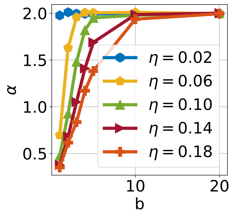
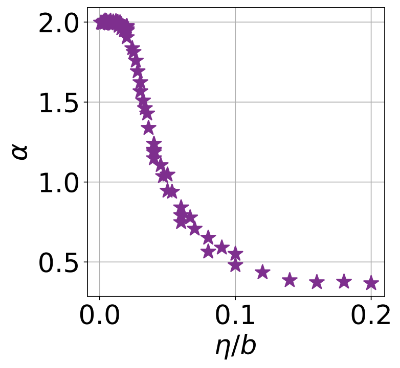
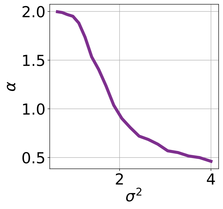
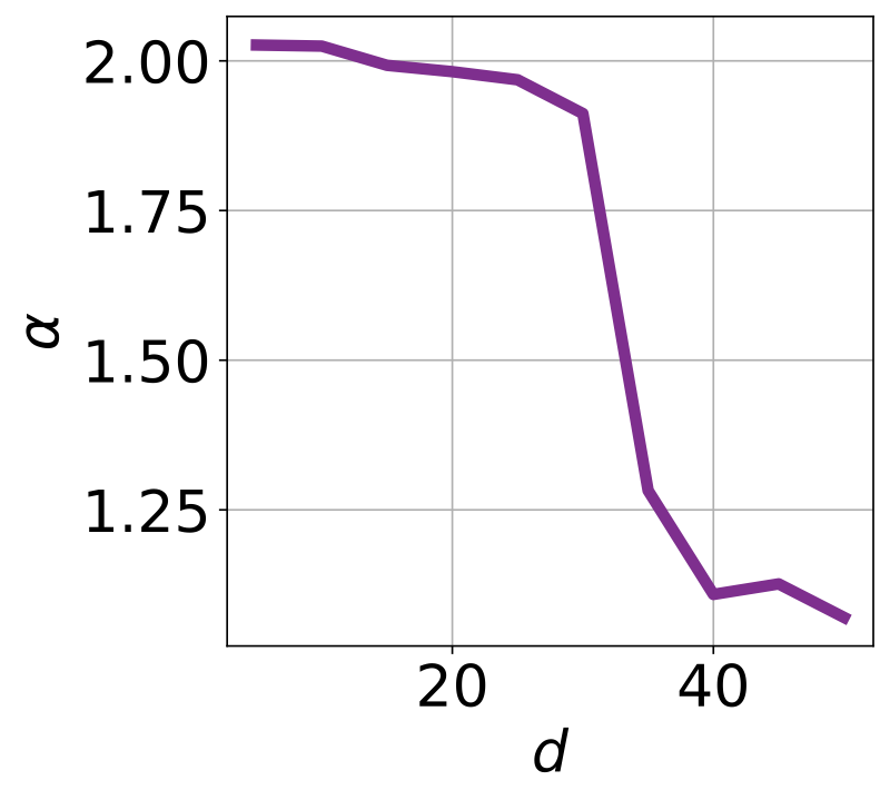
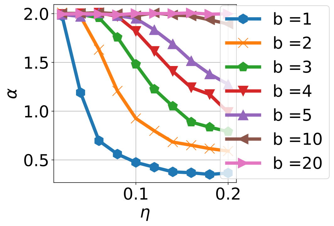
Figure 1: Behavior of $\alpha$ with (a) varying stepsize $\eta$ and batch-size $b$, (b) $d$ and $\sigma$, (c) under RMSProp.

To benefit from the GCLT, we are required to compute the average of the ‘centered’ iterates: $\frac{1}{K-K_{0}}\sum\nolimits_{k=K-K_{0}+1}^{K}(x_{k}-\bar{x})$, where $K_{0}$ is a ‘burn-in’ period aiming to discard the initial phase of SGD, and the mean of $\nu_{\infty}$ is given by $\bar{x}=\int_{\mathbb{R}^{d}}x\nu_{\infty}(dx)=(A^{\top}A)^{-1}A^{\top}y$ as long as $\alpha>1$, where the $i$-th row of $A\in\mathbb{R}^{n\times d}$ contains $a_{i}^{\top}$ and $y=[y_{1},\dots,y_{n}]\in\mathbb{R}^{n}$. We then repeat this procedure $1600$ times for different initial points and obtain $1600$ different random vectors, whose distributions are supposedly close to an $\alpha$-stable distribution. Finally, we run the tail-index estimator of Mohammadi et al. (2015) on these random vectors to estimate $\alpha$.

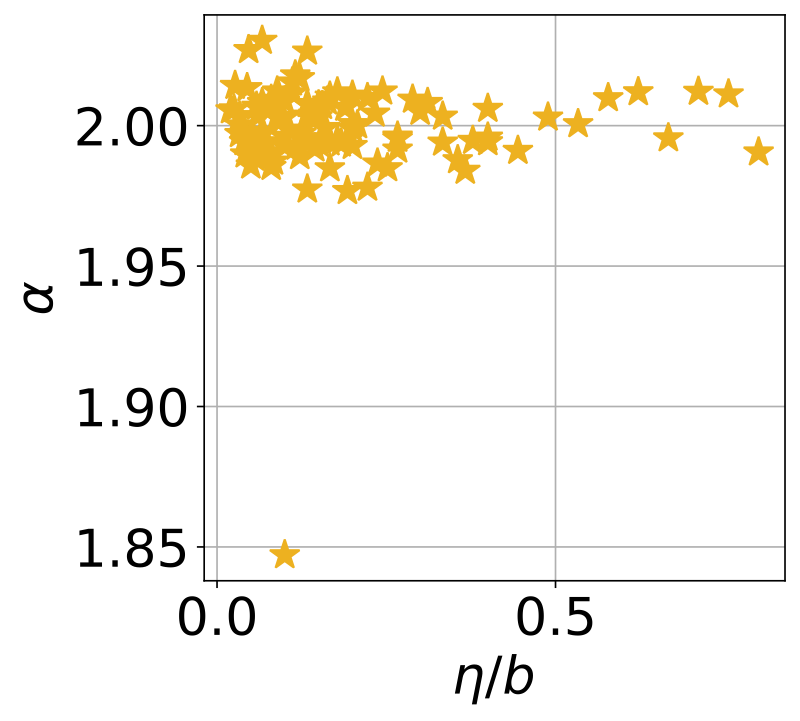
In our first experiment, we investigate the tail-index $\alpha$ of the stationary measure $\nu_{\infty}$ for varying stepsize $\eta$ and batch-size $b$. We set $d=100$ first fix the variances $\sigma=1$, $\sigma_{x}=\sigma_{y}=3$, and generate $\{a_{i},y_{i}\}_{i=1}^{n}$ by simulating the statistical model. Then, by fixing this dataset, we run the SGD recursion (3.5) for a large number of iterations and vary $\eta$ from $0.02$ to $0.2$ and $b$ from $1$ to $20$. We also set $K=1000$ and $K_{0}=500$. Figure 1 illustrates the results. We can observe that, increasing $\eta$ and decreasing $b$ both result in decreasing $\alpha$, where the tail-index can be prohibitively small (i.e., $\alpha<1$, hence even the mean of $\nu_{\infty}$ is not defined) for large $\eta$. Besides, we can also observe that the tail-index is in strong correlation with the ratio $\eta/b$.

In our second experiment, we investigate the effect of $d$ and $\sigma$ on $\alpha$. In Figure 1 (left), we set $d=100$, $\eta=0.1$ and $b=5$ and vary $\sigma$ from $0.8$ to $2$. For each value of $\sigma$, we simulate a new dataset from by using the generative model and run SGD with $K,K_{0}$. We again repeat each experiment $1600$ times. We follow a similar route for Figure 1 (right): we fix $\sigma=1.75$ and repeat the previous procedure for each value of $d$ ranging from $5$ to $50$. The results confirm our theory: $\alpha$ decreases for increasing $\sigma$ and $d$, and we observe that for a fixed $b$ and $\eta$ the change in $d$ can abruptly alter $\alpha$.

In our final synthetic data experiment, we investigate how the tails behave under adaptive optimization algorithms. We replicate the setting of our first experiment, with the only difference that we replace SGD with RMSProp (Hinton et al., 2012). As shown in Figure 1, the ‘clipping’ effect of RMSProp as reported in Zhang et al. (2020); Zhou et al. (2020) prevents the iterates become heavy-tailed and the vast majority of the estimated tail-indices is around $2$, indicating a Gaussian behavior. On the other hand, we repeated the same experiment with the variance-reduced optimization algorithm SVRG (Johnson and Zhang, 2013), and observed that for almost all choices of $\eta$ and $b$ the algorithm converges near the minimizer (with an error in the order of $10^{-6}$), hence the stationary distribution $\nu_{\infty}$ seems to be a degenerate distribution, which does not admit a heavy-tailed behavior. Regarding the link between heavy-tails and generalization (Martin and Mahoney, 2019; Şimşekli et al., 2020), this behavior of RMSProp and SVRG might be related to their ineffective generalization as reported in Keskar and Socher (2017); Defazio and Bottou (2019).

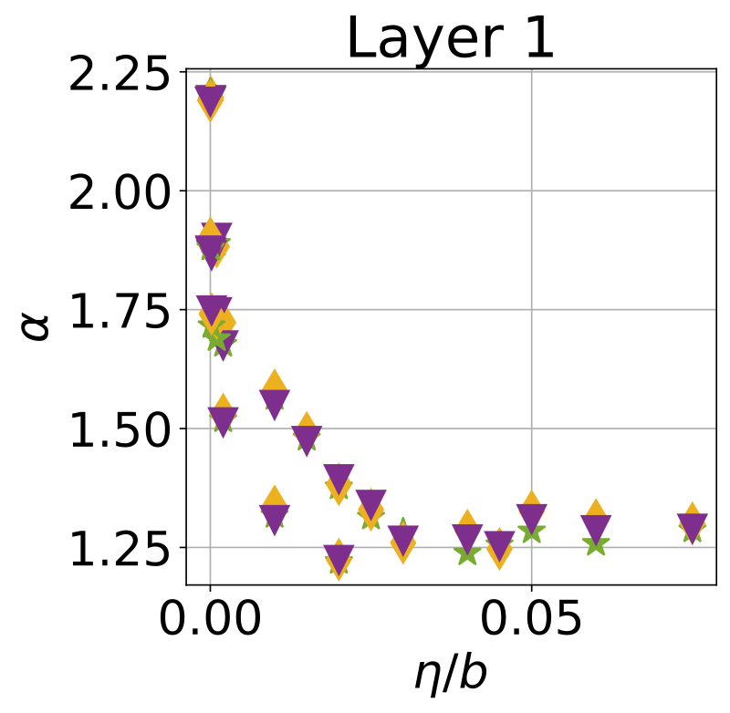
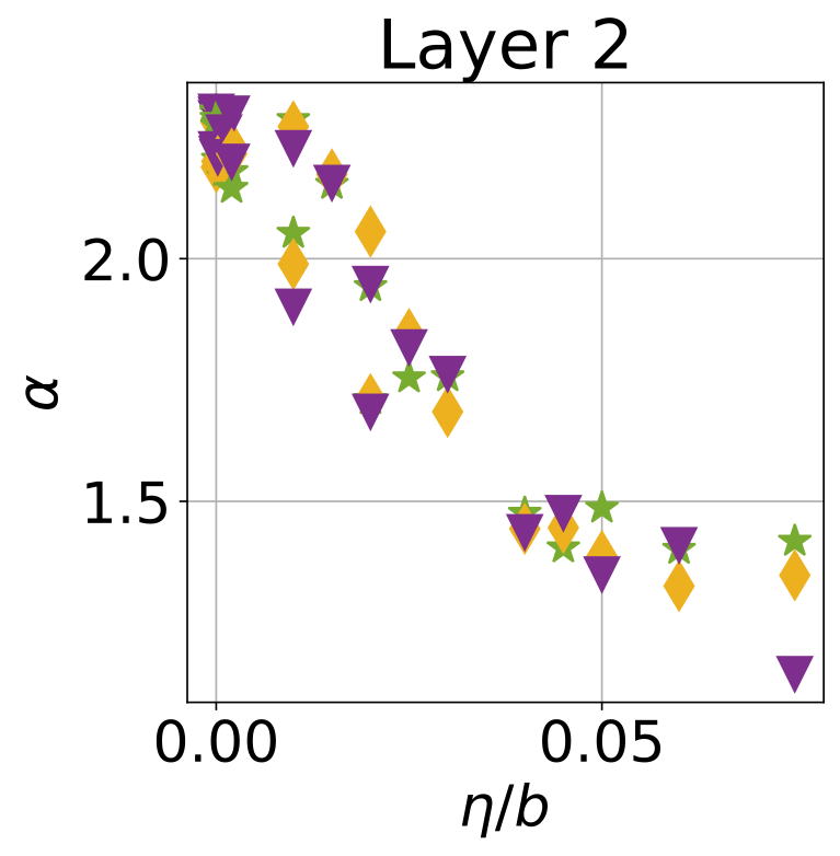
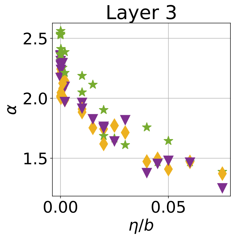
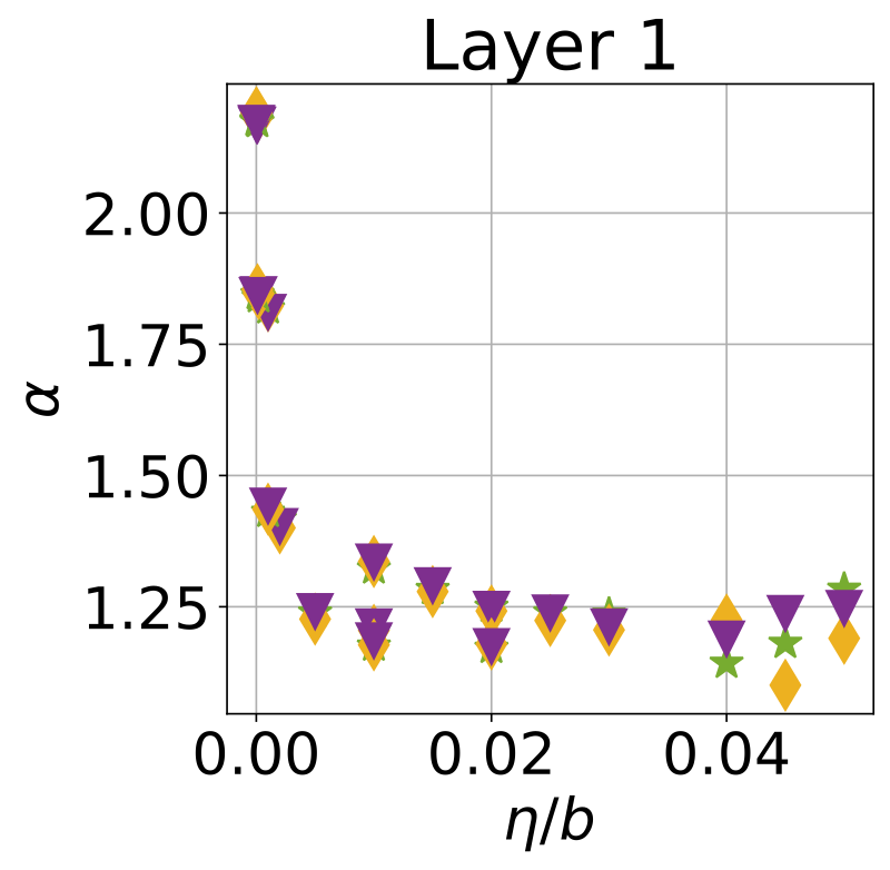
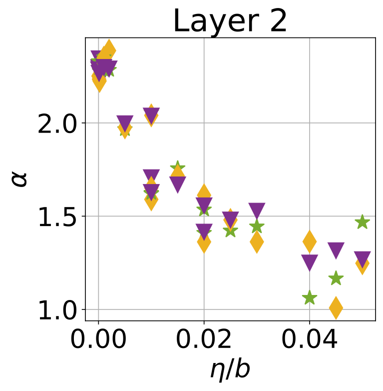
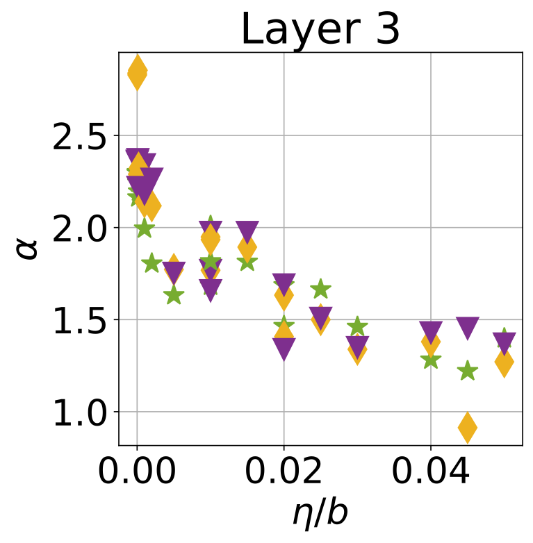
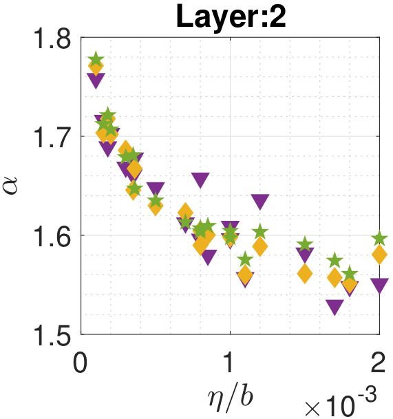
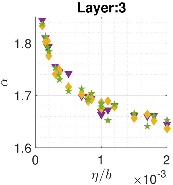
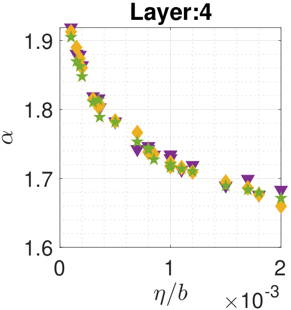
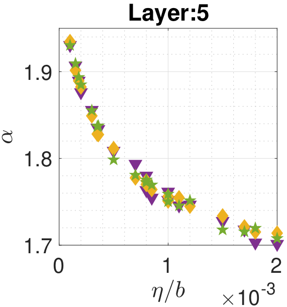
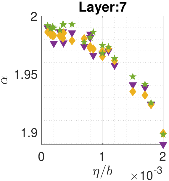
Experiments on fully connected neural networks. In the second set of experiments, we investigate the applicability of our theory beyond the quadratic optimization problems. Here, we follow the setup of Şimşekli et al. (2019a) and consider a fully connected neural network with the cross entropy loss and ReLU activation functions on the MNIST and CIFAR10 datasets. We train the models by using SGD for $10$K iterations and we range $\eta$ from $10^{-4}$ to $10^{-1}$ and $b$ from $1$ to $10$. Since it would be computationally infeasible to repeat each run thousands of times as we did in the synthetic data experiments, in this setting we follow a different approach based on (i) (Şimşekli et al., 2019a) that suggests that the tail behavior can differ in different layers of a neural network, and (ii) (De Bortoli et al., 2020) that shows that in the infinite width limit, the different components of a given layer of a two-layer fully connected network (FCN) becomes independent. Accordingly, we first compute the average of the last $1$K SGD iterates, whose distribution should be close an $\alpha$-stable distribution by the GCLT. We then treat each layer as a collection of i.i.d. $\alpha$-stable random variables and measure the tail-index of each individual layer separately by using the the estimator from Mohammadi et al. (2015). Figure 2 shows the results for a three-layer network (with $128$ hidden units at each layer) , whereas we obtained very similar results with a two-layer network as well. We observe that, while the dependence of $\alpha$ on $\eta/b$ differs from layer to layer, in each layer the measured $\alpha$ correlate very-well with the ratio $\eta/b$ in both datasets.

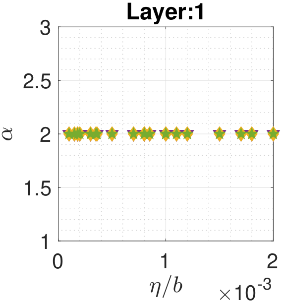
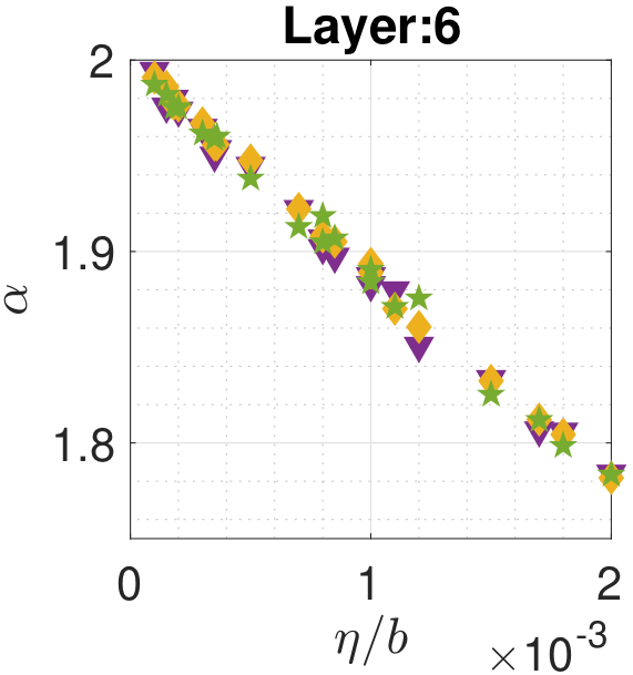
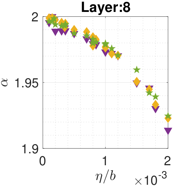
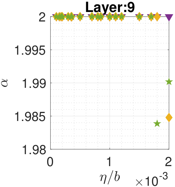
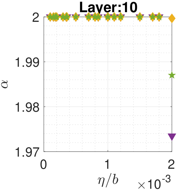
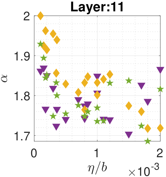
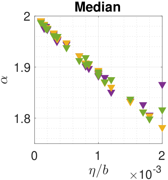
Experiments on VGG networks. In our last set of experiments, we evaluate our theory on VGG networks (Simonyan and Zisserman, 2015) on CIFAR10 with $11$ layers ($10$ convolutional layers with max-pooling and ReLU units, followed by a final linear layer), which contains $10$M parameters. We follow the same procedure as we used for the fully connected networks, where we vary $\eta$ from $10^{-4}$ to $1.7\times 10^{-3}$ and $b$ from $1$ to $10$. The results are shown in Figure 3. Similar to the previous experiments, we observe that $\alpha$ depends on the layers. For the layers 2-8, the tail-index correlates well with the ratio $\eta/b$, whereas the first and layers 1, 9, and 10 exhibit a Gaussian behavior ($\alpha\approx 2$). On the other hand, the correlation between the tail-index of the last layer (which is linear) with $\eta/b$ is still visible, yet less clear. Finally, in the last plot, we compute the median of the estimate tail-indices over layers, and observe a very clear decrease with increasing $\eta/b$. These observations provide further support for our theory and show that the heavy-tail phenomenon also occurs in neural networks, whereas $\alpha$ is potentially related to $\eta$ and $b$ in a more complicated way.

(a) MNIST

(b) CIFAR10

Figure 2: Results on FCNs. Different markers represent different initializations with the same $\eta$, $b$.

Figure 3: Results on VGG networks. The values of $\alpha$ that exceeded $2$ is truncated to $2$ for visualization purposes. Different markers represent different initializations.

5 Conclusion and Future Directions

We studied the tail behavior of SGD and showed that depending on $\eta$, $b$ and the curvature, the iterates can converge to a heavy-tailed random variable in distribution. We further supported our theory with various experiments conducted on neural networks and illustrated that our results would also apply to more general settings and hence provide new insights about the behavior of SGD in deep learning. Our study also brings up a number of future directions. (i) Our proof techniques are for the streaming setting, where each sample is used only once. Extending our results to the finite-sum scenario and investigating the effects of finite-sample size on the tail-index would be an interesting future research direction. (ii) We suspect that the tail-index may have an impact on the time required to escape a saddle point and this can be investigated further as another future research direction. (iii) Our work considers SGD with constant stepsize. Extending our analysis to adaptive methods and varying stepsizes is another interesting future research direction.

A A Note on Stochastic Differential Equation Representations for SGD

In recent years, a popular approach for analyzing the behavior of SGD has been viewing it as a discretization of a continuous-time stochastic process that can be represented via a stochastic differential equation (SDE) (Mandt et al., 2016; Jastrzębski et al., 2017; Li et al., 2017; Hu et al., 2019; Zhu et al., 2019; Chaudhari and Soatto, 2018; Şimşekli et al., 2019b). While these SDEs have been useful for understanding different properties of SGD, their differences and functionalities have not been clearly understood. In this section, in light of our theoretical results, we will discuss in which situation their choice would be more appropriate. We will restrict ourselves to the case where $f(x)$ is a quadratic function; however, the discussion can be extended to more general $f$.

The SDE approximations are often motivated by first rewriting the SGD recursion as follows:

$$x_{k+1}=x_{k}-\eta\nabla\tilde{f}_{k+1}\left(x_{k}\right)=x_{k}-\eta\nabla f\left(x_{k}\right)+\eta U_{k+1}(x_{k}),$$ (A.1)

where $U_{k}(x):=\nabla\tilde{f}_{k}(x)-\nabla f(x)$ is called the ‘stochastic gradient noise’. Then, based on certain statistical assumptions on $U_{k}$, we can view (A.1) as a discretization of an SDE. For instance, if we assume that the gradient noise follows a Gaussian distribution, whose covariance does not depend on the iterate $x_{k}$, i.e., $\eta U_{k}\approx\sqrt{\eta}Z_{k}$ where $Z_{k}\sim\mathcal{N}(0,\sigma_{z}\eta I)$ for some constant $\sigma_{z}>0$, we can see (A.1) as the Euler-Maruyama discretization of the following SDE with stepsize $\eta$ (Mandt et al., 2016):

$$\mathrm{d}x_{t}=-\nabla f(x_{t})\mathrm{d}t+\sqrt{\eta\sigma_{z}}\mathrm{d}\mathrm{B}_{t},$$ (A.2)

where $\mathrm{B}_{t}$ denotes the $d$-dimensional standard Brownian motion. This process is called the Ornstein-Uhlenbeck (OU) process (see e.g. Øksendal (2013)), whose invariant measure is a Gaussian distribution. We argue that this process can be a good proxy to (3.5) only when $\alpha\geq 2$, since otherwise the SGD iterates will exhibit heavy-tails, whose behavior cannot be captured by a Gaussian distribution. As we illustrated in Section 4, to obtain large $\alpha$, the stepsize $\eta$ needs to be small and/or the batch-size $b$ needs to be large. However, it is clear that this approximation will fall short when the system exhibits heavy tails, i.e., $\alpha<2$. Therefore, for the large $\eta/b$ regime, which appears to be more interesting since it often yields improved test performance (Jastrzębski et al., 2017), this approximation would be inaccurate for understanding the behavior of SGD. This problem mainly stems from the fact that the additive isotropic noise assumption results in a deterministic $M_{k}$ matrix for all $k$. Since there is no multiplicative noise term, this representation cannot capture a potential heavy-tailed behavior.

A natural extension of the state-independent Gaussian noise assumption is to incorporate the covariance structure of $U_{k}$. In our linear regression problem, we can easily see that the covariance matrix of the gradient noise has the following form:

$$\Sigma_{U}(x)=\mathrm{Cov}(U_{k}|x)=\frac{\sigma^{2}}{b}\mathrm{diag}(x\circ x),$$ (A.3)

where $\circ$ denotes element-wise multiplication and $\sigma^{2}$ is the variance of the data points. Therefore, we can extend the previous assumption by assuming $Z_{k}|x\sim\mathcal{N}(0,\eta\Sigma_{U}(x))$. It has been observed that this approximation yields a more accurate representation (Cheng et al., 2020; Ali et al., 2020; Jastrzębski et al., 2017). Using this assumption in (A.1), the SGD recursion coincides with the Euler-Maruyama discretization of the following SDE:

$$dx_{t} =-\nabla f(x_{t})dt+\sqrt{\eta\Sigma_{U}(x_{t})}d\mathrm{B}_{t}$$

$$\stackrel{{\scriptstyle\mathclap{\tiny\mbox{$\mathrm{d}$}}}}{{=}}-\left(A^{\top}Ax_{t}-A^{\top}y\right)dt+\sqrt{\frac{\sigma^{2}\eta}{b}}\mathrm{diag}(x_{t})d\mathrm{B}_{t},$$ (A.4)

where $\stackrel{{\scriptstyle\mathclap{\tiny\mbox{$\mathrm{d}$}}}}{{=}}$ denotes equality in distribution. The stochasticity in such SDEs is called often called multiplicative. Let us illustrate this property by discretizing this process and by using the definition of the gradient and the covariance matrix, we observe that (noting that $N_{k}\sim\mathcal{N}(0,I)$)

$$x_{k+1} =x_{k}-\eta\left(A^{\top}Ax_{k}-A^{\top}y\right)+\sqrt{\frac{\sigma^{2}\eta^{2}}{b}}\mathrm{diag}(x_{k})N_{k+1}$$

$$=\left(I-\eta A^{\top}A+\sqrt{\sigma^{2}\eta^{2}/b}\>\mathrm{diag}(N_{k+1})\right)x_{k}-\eta A^{\top}y,$$ (A.5)

where we can clearly see the multiplicative effect of the noise, as indicated by its name. On the other hand, we can observe that, thanks to the multiplicative structure, this process would be able to capture the potential heavy-tailed structure of SGD. However, there are two caveats. The first one is that, in the case of linear regression, the process is called a geometric (or modified) Ornstein-Uhlenbeck process which is an extension of geometric Brownian motion. One can show that the distribution of the process at any time $t$ will have lognormal tails. Hence it will be accurate only when the tail-index $\alpha$ is close to the one of the lognormal distribution. The second caveat is that, for a more general cost function $f$, the covariance matrix is more complicated and hence the invariant measure of the process cannot be found analytically, hence analyzing these processes for a general $f$ can be as challenging as directly analyzing the behavior of SGD.

The third way of modeling the gradient noise is based on assuming that it is heavy-tailed. In particular, we can assume that $\eta U_{k}\approx\eta^{1/\alpha}L_{k}$ where $[L_{k}]_{i}\sim\mathcal{S}\alpha\mathcal{S}(\sigma_{L}\eta^{(\alpha-1)/\alpha})$ for all $i=1,\dots,d$. Under this assumption the SGD recursion coincides with the Euler discretization of the following Lévy-driven SDE (Şimşekli et al., 2019b):

$$dx_{t}=-\nabla f(x_{t})dt+\sigma_{L}\eta^{(\alpha-1)/\alpha}d\mathrm{L}^{\alpha}_{t},$$ (A.6)

where $\mathrm{L}^{\alpha}_{t}$ denotes the $\alpha$-stable Lévy process with independent components (see Section A.1 for technical background on Lévy processes and in particular $\alpha$-stable Lévy processes). In the case of linear regression, this processes is called a fractional OU process (Fink and Klüppelberg, 2011), whose invariant measure is also an $\alpha$-stable distribution with the same tail-index $\alpha$. Hence, even though it is based on an isotropic, state-independent noise assumption, in the case of large $\eta/b$ regime, this approach can mimic the heavy-tailed behavior of the system with the exact tail-index $\alpha$. On the other hand, Buraczewski et al. (2016) (Theorem 1.7 and 1.16) showed that if $U_{k}$ is assumed to heavy tailed with index $\alpha$ (not necessarily $\mathcal{S}\alpha\mathcal{S}$) then the process $x_{k}$ will inherit the same tails and the ergodic averages will still converge to an $\mathcal{S}\alpha\mathcal{S}$ random variable in distribution, hence generalizing the conclusions of the $\mathcal{S}\alpha\mathcal{S}$ assumption to the case where $U_{k}$ follows an arbitrary heavy-tailed distribution.

A.1 Technical background: Lévy processes

Lévy motions (processes) are stochastic processes with independent and stationary increments, which include Brownian motions as a special case, and in general may have heavy-tailed distributions (see e.g. Bertoin (1996) for a survey). Symmetric $\alpha$-stable Lévy motion is a Lévy motion whose time increments are symmetric $\alpha$-stable distributed. We define $\mathrm{L}^{\alpha}_{t}$, a $d$-dimensional symmetric $\alpha$-stable Lévy motion as follows. Each component of $\mathrm{L}^{\alpha}_{t}$ is an independent scalar $\alpha$-stable Lévy process defined as follows:

(i) $\mathrm{L}^{\alpha}_{0}=0$ almost surely;

(ii) For any $t_{0}<t_{1}<\cdots<t_{N}$, the increments $\mathrm{L}^{\alpha}_{t_{n}}-\mathrm{L}^{\alpha}_{t_{n-1}}$ are independent, $n=1,2,\ldots,N$;

(iii) The difference $\mathrm{L}^{\alpha}_{t}-\mathrm{L}^{\alpha}_{s}$ and $\mathrm{L}^{\alpha}_{t-s}$ have the same distribution: $\mathcal{S}\alpha\mathcal{S}((t-s)^{1/\alpha})$ for $s<t$;

(iv) $\mathrm{L}^{\alpha}_{t}$ has stochastically continuous sample paths, i.e. for any $\delta>0$ and $s\geq 0$, $\mathbb{P}(|\mathrm{L}^{\alpha}_{t}-\mathrm{L}^{\alpha}_{s}|>\delta)\rightarrow 0$ as $t\rightarrow s$.

When $\alpha=2$, we obtain a scaled Brownian motion as a special case, i.e. $\mathrm{L}^{\alpha}_{t}=\sqrt{2}\mathrm{B}_{t}$, so that the difference $\mathrm{L}^{\alpha}_{t}-\mathrm{L}^{\alpha}_{s}$ follows a Gaussian distribution $\mathcal{N}(0,2(t-s))$.

B Tail-Index Estimation

In this study, we follow Tzagkarakis et al. (2018); Şimşekli et al. (2019b), and make use of the recent estimator proposed by Mohammadi et al. (2015).

Theorem 12 (Mohammadi et al. (2015) Corollary 2.4)

Let $\{X_{i}\}_{i=1}^{K}$ be a collection of strictly stable random variables in $\mathbb{R}^{d}$ with tail-index $\alpha\in(0,2]$ and $K=K_{1}\times K_{2}$. Define $Y_{i}=\sum_{j=1}^{K_{1}}X_{j+(i-1)K_{1}}\>$ for $i\in\llbracket 1,K_{2}\rrbracket$. Then, the estimator

$$\widehat{\phantom{a}\frac{1}{\alpha}\phantom{a}}\triangleq\frac{1}{\log K_{1}}\Bigl{(}\frac{1}{K_{2}}\sum_{i=1}^{K_{2}}\log\|Y_{i}\|-\frac{1}{K}\sum_{i=1}^{K}\log\|X_{i}\|\Bigr{)},$$ (B.1)

converges to $1/{\alpha}$ almost surely, as $K_{2}\rightarrow\infty$.

As this estimator requires a hyperparameter $K_{1}$, at each tail-index estimation, we used several values for $K_{1}$ and we used the median of the estimators obtained with different values of $K_{1}$. We provide the codes in github.com/umutsimsekli/sgd_ht, where the implementation details can be found. For the neural network experiments, we used the same setup as provided in the repository of Şimşekli et al. (2019b).

C Proofs of Main Results

C.1 Proof of Theorem 2

Proof The proof follows from Theorem 4.4.15 in Buraczewski et al. (2016) which goes back to Theorem 1.1 in Alsmeyer and Mentemeier (2012) and Theorem 6 in Kesten (1973). See also Goldie (1991); Buraczewski et al. (2015). We recall that we have the stochastic recursion:

$$x_{k}=M_{k}x_{k-1}+q_{k},$$ (C.1)

where the sequence $(M_{k},q_{k})$ are i.i.d. distributed as $(M,q)$ and for each $k$, $(M_{k},q_{k})$ is independent of $x_{k-1}$. To apply Theorem 4.4.15 in Buraczewski et al. (2016), it suffices to have the following conditions being satisfied:

1. $M$ is invertible with probability 1.

2. The matrix $M$ has a continuous Lebesgue density that is positive in a neighborhood of the identity matrix.

3. $\rho<0$ and $h(\alpha)=1$.

4. $\mathbb{P}(Mx+q=x)<1$ for every $x$.

5. $\mathbb{E}\left[\|M\|^{\alpha}(\log^{+}\|M\|+\log^{+}\|M^{-1}\|)\right]<\infty$.

6. $0<\mathbb{E}\|q\|^{\alpha}<\infty$.

All the conditions are satisfied under our assumptions. In particular, Condition 1 and Condition 5 are proved in Lemma 21, and Condition 2 and Condition 4 follow from the fact that $M$ and $q$ have continuous distributions. Condition 3 is part of the assumption of Theorem 2. Finally, Condition 6 is satisfied by the definition of $q$ and by the Assumptions (A1)–(A2).  

C.2 Proof of Theorem 3

Proof To prove (i), according to the proof of Theorem 2, it suffices to show that if $\rho<0$, then there exists a unique positive $\alpha$ such that $h(\alpha)=1$. Note that if $\rho<0$, then by Lemma 17, we have $h(0)=1$, $h^{\prime}(0)=\rho<0$ and $h(s)$ is convex in $s$, and moreover by Lemma 18, we have $\liminf_{s\rightarrow\infty}h(s)>1$. Therefore, there exists some $\alpha\in(0,\infty)$ such that $h(\alpha)=1$. Finally, (ii) follows from Lemma 16.  

C.3 Proof of Theorem 4

Proof We will split the proof of Theorem 4 into two parts:

(I) We will show that the tail-index $\alpha$ is strictly decreasing in stepsize $\eta$ and variance $\sigma^{2}$ provided that $\alpha\geq 1$.

(II) We will show that the tail-index $\alpha$ is strictly increasing in batch-size $b$ provided that $\alpha\geq 1$.

(III) We will show that the tail-index $\alpha$ is strictly decreasing in dimension $d$.

First, let us prove (I). Let $a:=\eta\sigma^{2}>0$ be given. Consider the tail-index $\alpha$ as a function of $a$, i.e.

$$\alpha(a):=\min\{s:h(a,s)=1\}\,,$$

where $h(a,s)=h(s)$ with emphasis on dependence on $a$.

By assumption, $\alpha(a)\geq 1$. The function $h(a,s)$ is convex function of $a$ (see Lemma 22 for $s\geq 1$ and a strictly convex function of $s$ for $s\geq 0$). Furthermore, it satisfies $h(a,0)=1$ for every $a\geq 0$ and $h(0,s)=1$ for every $s\geq 0$. We consider the curve

$$\mathcal{C}:=\left\{(a,s)\in(0,\infty)\times[1,\infty]:h(a,s)=1\right\}.$$

This is the set of the choice of $a$, which leads to a tail-index $s$ where $s\geq 1$. Since $h$ is smooth in both $a$ and $s$, we can represent $s$ as a smooth function of $a$, i.e. on the curve

$$h(a,s(a))=0\,,$$

where $s(a)$ is a smooth function of $a$. We will show that $s^{\prime}(a)<0$; i.e. if we increase $a$; the tail-index $s(a)$ will drop. Pick any $(a_{*},s_{*})\in\mathcal{C}$, it will satisfy $h(a_{*},s_{*})=1$. We have the following facts:

• The function $h(a,s)=1$ for either $a=0$ or $s=0$. This is illustrated in Figure 4 with a blue marker.

• $h(a_{*},s)<1$ for $s<s_{*}$. This follows from the convexity of $h(a_{*},s)$ function and the fact that $h(a_{*},0)=1$, $h(a_{*},s_{*})=1$. From here, we see that the function $h(a_{*},s)$ is increasing at $s=s_{*}$ and we have its derivative

  $$\frac{\partial h}{\partial s}(a_{*},s_{*})>0.$$

• The function $h(a,s_{*})$ is convex as a function of $a$ by Lemma 22, it satisfies $h(0,s_{*})=h(a_{*},s_{*})=1$. Therefore, by convexity $h(a,s_{*})<1$ for a $\in(0,s_{*})$; otherwise the function $h(a,s_{*})$ would be a constant function. We have therefore necessarily.

  $$\frac{\partial h}{\partial a}(a_{*},s_{*})>0.$$

  By convexity of the function $h(a,s_{*})$, we have also $h(a,s_{*})\geq h(a_{*},s_{*})+\frac{\partial h}{\partial a}(a_{*},s_{*})(a-a_{*})>h(a_{*},s_{*})=1$. Therefore, $h(a,s_{*})>1$ for $a>a_{*}$. Then, it also follows that $h(a,s)>1$ for $a>a_{*}$ and $s>s_{*}$ (otherwise if $h(a,s)\leq 1$, we get a contradiction because $h(0,s)=1$, $h(a_{*},s)>1$ and $h(a,s)\leq 1$ is impossible due to convexity). This is illustrated in Figure 4 where we mark this region as a rectangular box where $h>1$.

  

  Figure 4: The curve $h(a,s)=1$ in the $(a,s)$ plane

• By similar arguments we can show that the function $h(a,s)<1$ if $(s,a)\in(0,a_{*})\times[1,s_{*})$. Indeed, if $h(a,s)\geq 1$ for some $(s,a)\in[1,s_{*})\times(0,a_{*})$, this contradicts the fact that $h(0,s)=1$ and $h(a_{*},s)<1$ proven in part $(ii)$. This is illustrated in Figure 4 where inside the rectangular box on the left-hand side, we have $h<1$.

Geometrically, we see from Figure 4 that the curve $s(a)$ as a function of $a$, is sandwiched between two rectangular boxes and has necessarily $s^{\prime}(a)<0$. This can also be directly obtained rigorously from the implicit function theorem; if we differentiate the implicit equation $h(a,s(a))=0$ with respect to $a$, we obtain

$$\frac{\partial h}{\partial a}(a_{*},s_{*})+\frac{\partial h}{\partial s}(a_{*},s_{*})s^{\prime}(a_{*})=0\,.$$

From parts $(ii)-(iii)$, we have $\frac{\partial h}{\partial a}(a_{*},s_{*})$ and $\frac{\partial h}{\partial s}(a_{*},s_{*})>0$. Therefore, we have

$$s^{\prime}(a_{*})=-\frac{\frac{\partial h}{\partial a}(a_{*},s_{*})}{\frac{\partial h}{\partial s}(a_{*},s_{*})}<0\,,$$ (C.2)

which completes the proof for $s_{*}\geq 1$.

Next, let us prove (II). With slight abuse of notation, we define the function $h(b,s)=h(s)$ to emphasize the dependence on $b$. We have

$$h(b,s)=\mathbb{E}\left\|\left(I-\frac{\eta}{b}\sum_{i=1}^{b}a_{i}a_{i}^{T}\right)e_{1}\right\|^{s}.$$ (C.3)

where we used Lemma 16. When $s\geq 1$, the function $x\mapsto\|x\|^{s}$ is convex, and by Jensen’s inequality, we get for any $b\geq 2$ and $b\in\mathbb{N}$,

$$h(b,s) =\mathbb{E}\left\|\frac{1}{b}\sum_{i=1}^{b}\left(I-\frac{\eta}{b-1}\sum_{j\neq i}a_{j}a_{j}^{T}\right)e_{1}\right\|^{s}$$

$$\leq\mathbb{E}\left[\frac{1}{b}\sum_{i=1}^{b}\left\|\left(I-\frac{\eta}{b-1}\sum_{j\neq i}a_{j}a_{j}^{T}\right)e_{1}\right\|^{s}\right]$$

$$=\frac{1}{b}\sum_{i=1}^{b}\mathbb{E}\left[\left\|\left(I-\frac{\eta}{b-1}\sum_{j\neq i}a_{j}a_{j}^{T}\right)e_{1}\right\|^{s}\right]=h(b-1,s),$$

where we used the fact that $a_{i}$ are i.i.d. Indeed, from the condition for equality to hold in Jensen’s inequality, and the fact that $a_{i}$ are i.i.d. random, the inequality above is a strict inequality. Hence when $d\in\mathbb{N}$ for any $s\geq 1$, $h(b,s)$ is strictly decreasing in $b$. By following the same argument as in the proof of (I), we conclude that the tail-index $\alpha$ is strictly increasing in batch-size $b$.

Finally, let us prove (III). Let us show the tail-index $\alpha$ is strictly decreasing in dimension $d$. Since $a_{i}$ are i.i.d. and $a_{i}\sim\mathcal{N}(0,\sigma^{2}I_{d})$, by Lemma 19,

$$h(s)=\mathbb{E}\left[\left(1-\frac{2a}{b}X+\frac{a^{2}}{b^{2}}X^{2}+\frac{a^{2}}{b^{2}}XY\right)^{s/2}\right],$$ (C.4)

where $X,Y$ are independent chi-square random variables with degree of freedom $b$ and $d-1$ respectively. Notice that $h(s)$ is strictly increasing in $d$ since the only dependence of $h(s)$ on $d$ is via $Y$, which is a chi-square distribution with degree of freedom $(d-1)$. By writing $Y=Z_{1}^{2}+\cdots+Z_{d-1}^{2}$, where $Z_{i}\sim N(0,1)$ i.i.d., it follows that $h(s)$ is strictly increasing in $d$. Hence, by similar argument as in (I), we conclude that $\alpha$ is strictly decreasing in dimension $d$.  

Remark 13

When $d=1$ and $a_{i}$ are i.i.d. $N(0,\sigma^{2})$, we can provide an alternative proof that the tail-index $\alpha$ is strictly increasing in batch-size $b$. It suffices to show that for any $s\geq 1$, $h(s)$ is strictly decreasing in the batch-size $b$. By Lemma 19 when $d=1$,

$$h(b,s)=\mathbb{E}\left[\left(1-\frac{2\eta\sigma^{2}}{b}X+\frac{\eta^{2}\sigma^{4}}{b^{2}}X^{2}+\frac{\eta^{2}\sigma^{4}}{b^{2}}XY\right)^{s/2}\right],$$ (C.5)

where $h(b,s)$ is as in (C.3) and $X,Y$ are independent chi-square random variables with degree of freedom $b$ and $d-1$ respectively. When $d=1$, we have $Y\equiv 0$, and

$$h(b,s)=\mathbb{E}\left[\left(1-\frac{2\eta\sigma^{2}}{b}X+\frac{\eta^{2}\sigma^{4}}{b^{2}}X^{2}\right)^{s/2}\right]=\mathbb{E}\left[\left|1-\frac{\eta\sigma^{2}}{b}X\right|^{s}\right].$$ (C.6)

Since $X$ is a chi-square random variable with degree of freedom $b$, we have

$$h(b,s)=\mathbb{E}\left[\left|1-\frac{\eta\sigma^{2}}{b}\sum_{i=1}^{b}Z_{i}\right|^{s}\right],$$ (C.7)

where $Z_{i}$ are i.i.d. $N(0,1)$ random variables. When $s\geq 1$, the function $x\mapsto|x|^{s}$ is convex, and by Jensen’s inequality, we get for any $b\geq 2$ and $b\in\mathbb{N}$

$$h(b,s) =\mathbb{E}\left[\left|\frac{1}{b}\sum_{i=1}^{b}\left(1-\frac{\eta\sigma^{2}}{b-1}\sum_{j\neq i}Z_{j}\right)\right|^{s}\right]$$

$$\leq\mathbb{E}\left[\frac{1}{b}\sum_{i=1}^{b}\left|1-\frac{\eta\sigma^{2}}{b-1}\sum_{j\neq i}Z_{j}\right|^{s}\right]=\frac{1}{b}\sum_{i=1}^{b}\mathbb{E}\left[\left|1-\frac{\eta\sigma^{2}}{b-1}\sum_{j\neq i}Z_{j}\right|^{s}\right]=h(b-1,s),$$

where we used the fact that $Z_{i}$ are i.i.d. Indeed, from the condition for equality to hold in Jensen’s inequality, and the fact that $Z_{i}$ are i.i.d. $N(0,1)$ distributed, the inequality above is a strict inequality. Hence when $d=1$ for any $s\geq 1$, $h(b,s)$ is strictly decreasing in $b$.

C.4 Proof of Proposition 5

Proof We first prove (i). When $\eta=\eta_{crit}=\frac{2b}{\sigma^{2}(d+b+1)}$, that is $\eta\sigma^{2}(d+b+1)=2b$, we can compute that

$$\rho\leq\frac{1}{2}\log\mathbb{E}\left[1-\frac{2\eta\sigma^{2}}{b}\sum_{i=1}^{b}z_{i1}^{2}+\frac{\eta^{2}\sigma^{4}}{b^{2}}\sum_{i=1}^{b}\sum_{j=1}^{b}(z_{i1}z_{j1}+\cdots+z_{id}z_{jd})z_{i1}z_{j1}\right]=0,$$ (C.8)

where $z_{ij}$ are i.i.d. $N(0,1)$ random variables. Note that since

$$1-\frac{2\eta\sigma^{2}}{b}\sum_{i=1}^{b}z_{i1}^{2}+\frac{\eta^{2}\sigma^{4}}{b^{2}}\sum_{i=1}^{b}\sum_{j=1}^{b}(z_{i1}z_{j1}+\cdots+z_{id}z_{jd})z_{i1}z_{j1}$$

is random, the inequality above is a strict inequality from Jensen’s inequality. Thus, when $\eta=\eta_{crit}$, i.e. $\eta\sigma^{2}(d+b+1)=2b$, $\rho<0$. By continuity, there exists some $\delta>0$ such that for any $2b<\eta\sigma^{2}(d+b+1)<2b+\delta$, i.e. $\eta_{crit}<\eta<\eta_{max}$, where $\eta_{max}:=\eta_{crit}+\frac{\delta}{\sigma^{2}(d+b+1)}$, we have $\rho<0$. Moreover, when $\eta\sigma^{2}(d+b+1)>2b$, i.e. $\eta>\eta_{crit}$, we have

$$h(2) = \mathbb{E}\left[\bigg{(}1-\frac{2\eta\sigma^{2}}{b}\sum_{i=1}^{b}z_{i1}^{2}+\frac{\eta^{2}\sigma^{4}}{b^{2}}\sum_{i=1}^{b}\sum_{j=1}^{b}(z_{i1}z_{j1}+\cdots+z_{id}z_{jd})z_{i1}z_{j1}\bigg{)}\right]$$

$$= 1-2\eta\sigma^{2}+\frac{\eta^{2}\sigma^{4}}{b}(d+b+1)\geq 1,$$

which implies that there exists some $0<\alpha<2$ such that $h(\alpha)=1$.

Finally, let us prove (ii) and (iii). When $\eta\sigma^{2}(d+b+1)\leq 2b$, i.e. $\eta\leq\eta_{crit}$, we have $h(2)\leq 1$, which implies that $\alpha>2$. In particular, when $\eta\sigma^{2}(d+b+1)=2b$, i.e. $\eta=\eta_{crit}$, the tail-index $\alpha=2$.  

C.5 Proof of Theorem 6 and Corollary 7

C.5.1 Proof of Theorem 6

Proof We recall that

$$x_{k}=M_{k}x_{k-1}+q_{k},$$ (C.9)

which implies that

$$\|x_{k}\|\leq\|M_{k}x_{k-1}\|+\|q_{k}\|.$$ (C.10)

(i) If the tail-index $\alpha\leq 1$, then for any $0<p<\alpha$, we have $h(p)=\mathbb{E}\|M_{k}e_{1}\|^{p}<1$ and moreover by Lemma 23,

$$\|x_{k}\|^{p}\leq\|M_{k}x_{k-1}\|^{p}+\|q_{k}\|^{p}.$$ (C.11)

Due to spherical symmetry of the isotropic Gaussian distribution, the distribution of $\frac{\|M_{k}x\|}{\|x\|}$ does not depend on the choice of $x\in\mathbb{R}^{d}\backslash\{0\}$. Therefore, $\frac{\|M_{k}x_{k-1}\|}{\|x_{k-1}\|}$ and $\|x_{k-1}\|$ are independent, and $\frac{\|M_{k}x_{k-1}\|}{\|x_{k-1}\|}$ has the same distribution as $\|M_{k}e_{1}\|$, where $e_{1}$ is the first basis vector. It follows that

$$\mathbb{E}\|x_{k}\|^{p}\leq\mathbb{E}\|M_{k}e_{1}\|^{p}\mathbb{E}\|x_{k-1}\|^{p}+\mathbb{E}\|q_{k}\|^{p},$$ (C.12)

so that

$$\mathbb{E}\|x_{k}\|^{p}\leq h(p)\mathbb{E}\|x_{k-1}\|^{p}+\mathbb{E}\|q_{1}\|^{p},$$ (C.13)

where $h(p)\in(0,1)$. By iterating over $k$, we get

$$\mathbb{E}\|x_{k}\|^{p}\leq(h(p))^{k}\mathbb{E}\|x_{0}\|^{p}+\frac{1-(h(p))^{k}}{1-h(p)}\mathbb{E}\|q_{1}\|^{p}.$$ (C.14)

(ii) If the tail-index $\alpha>1$, then for any $1<p<\alpha$, by Lemma 23, for any $\epsilon>0$, we have

$$\|x_{k}\|^{p}\leq(1+\epsilon)\|M_{k}x_{k-1}\|^{p}+\frac{(1+\epsilon)^{\frac{p}{p-1}}-(1+\epsilon)}{\left((1+\epsilon)^{\frac{1}{p-1}}-1\right)^{p}}\|q_{k}\|^{p},$$ (C.15)

which (similar as in (i)) implies that

$$\mathbb{E}\|x_{k}\|^{p}\leq(1+\epsilon)\mathbb{E}\|M_{k}e_{1}\|^{p}\mathbb{E}\|x_{k-1}\|^{p}+\frac{(1+\epsilon)^{\frac{p}{p-1}}-(1+\epsilon)}{\left((1+\epsilon)^{\frac{1}{p-1}}-1\right)^{p}}\mathbb{E}\|q_{k}\|^{p},$$ (C.16)

so that

$$\mathbb{E}\|x_{k}\|^{p}\leq(1+\epsilon)h(p)\mathbb{E}\|x_{k-1}\|^{p}+\frac{(1+\epsilon)^{\frac{p}{p-1}}-(1+\epsilon)}{\left((1+\epsilon)^{\frac{1}{p-1}}-1\right)^{p}}\mathbb{E}\|q_{1}\|^{p}.$$ (C.17)

We choose $\epsilon>0$ so that $(1+\epsilon)h(p)<1$. By iterating over $k$, we get

$$\mathbb{E}\|x_{k}\|^{p}\leq((1+\epsilon)h(p))^{k}\mathbb{E}\|x_{0}\|^{p}+\frac{1-((1+\epsilon)h(p))^{k}}{1-(1+\epsilon)h(p)}\frac{(1+\epsilon)^{\frac{p}{p-1}}-(1+\epsilon)}{\left((1+\epsilon)^{\frac{1}{p-1}}-1\right)^{p}}\mathbb{E}\|q_{1}\|^{p}.$$ (C.18)

The proof is complete.  

Remark 14

In general, there is no closed-form expression for $\mathbb{E}\|q_{1}\|^{p}$ in Theorem 6. We provide an upper bound as follows. When $p>1$, by Jensen’s inequality, we can compute that

$$\mathbb{E}\|q_{1}\|^{p}=\eta^{p}\mathbb{E}\left\|\frac{1}{b}\sum_{i=1}^{b}a_{i}y_{i}\right\|^{p}\leq\frac{\eta^{p}}{b}\sum_{i=1}^{b}\mathbb{E}\left\|a_{i}y_{i}\right\|^{p}=\eta^{p}\mathbb{E}\left[|y_{1}|^{p}\left\|a_{1}\right\|^{p}\right],$$ (C.19)

and when $p\leq 1$, by Lemma 23, we can compute that

$$\mathbb{E}\|q_{1}\|^{p}=\frac{\eta^{p}}{b^{p}}\mathbb{E}\left\|\sum_{i=1}^{b}a_{i}y_{i}\right\|^{p}\leq\frac{\eta^{p}}{b^{p}}\mathbb{E}\left[\left(\sum_{i=1}^{b}\left\|a_{i}y_{i}\right\|\right)^{p}\right]\leq\frac{\eta^{p}}{b^{p}}\sum_{i=1}^{b}\mathbb{E}\left\|a_{i}y_{i}\right\|^{p}=\eta^{p}\mathbb{E}\left[|y_{1}|^{p}\left\|a_{1}\right\|^{p}\right].$$ (C.20)

C.5.2 Proof of Corollary 7

Proof It follows from Theorem 6 by letting $k\rightarrow\infty$ and applying Fatou’s lemma.  

C.6 Proof of Theorem 8, Corollary 9, Proposition 10 and Corollary 11

C.6.1 Proof of Theorem 8

Proof For any $\nu_{0},\tilde{\nu}_{0}\in\mathcal{P}_{p}(\mathbb{R}^{d})$, there exists a couple $x_{0}\sim\nu_{0}$ and $\tilde{x}_{0}\sim\tilde{\nu}_{0}$ independent of $(M_{k},q_{k})_{k\in\mathbb{N}}$ and $\mathcal{W}_{p}^{p}(\nu_{0},\tilde{\nu}_{0})=\mathbb{E}\|x_{0}-\tilde{x}_{0}\|^{p}$. We define $x_{k}$ and $\tilde{x}_{k}$ starting from $x_{0}$ and $\tilde{x}_{0}$ respectively, via the iterates

$$x_{k}=M_{k}x_{k-1}+q_{k},$$ (C.21)

$$\tilde{x}_{k}=M_{k}\tilde{x}_{k-1}+q_{k},$$ (C.22)

and let $\nu_{k}$ and $\tilde{\nu}_{k}$ denote the probability laws of $x_{k}$ and $\tilde{x}_{k}$ respectively. For any $p<\alpha$, since $\mathbb{E}\|M_{k}\|^{\alpha}=1$ and $\mathbb{E}\|q_{k}\|^{\alpha}<\infty$, we have $\nu_{k},\tilde{\nu}_{k}\in\mathcal{P}_{p}(\mathbb{R}^{d})$ for any $k$. Moreover, we have

$$x_{k}-\tilde{x}_{k}=M_{k}(x_{k-1}-\tilde{x}_{k-1}),$$ (C.23)

Due to spherical symmetry of the isotropic Gaussian distribution, the distribution of $\frac{\|M_{k}x\|}{\|x\|}$ does not depend on the choice of $x\in\mathbb{R}^{d}\backslash\{0\}$. Therefore, $\frac{\|M_{k}(x_{k-1}-\tilde{x}_{k-1})\|}{\|x_{k-1}-\tilde{x}_{k-1}\|}$ and $\|x_{k-1}-\tilde{x}_{k-1}\|$ are independent, and $\frac{\|M_{k}(x_{k-1}-\tilde{x}_{k-1})\|}{\|x_{k-1}-\tilde{x}_{k-1}\|}$ has the same distribution as $\|M_{k}e_{1}\|$, where $e_{1}$ is the first basis vector. It follows from (C.23) that

$$\mathbb{E}\|x_{k}-\tilde{x}_{k}\|^{p}\leq\mathbb{E}\left[\|M_{k}(x_{k-1}-\tilde{x}_{k-1})\|^{p}\right] = \mathbb{E}\left[\|M_{k}e_{1}\|^{p}\right]\mathbb{E}\left[\|x_{k-1}-\tilde{x}_{k-1}\|^{p}\right]$$

$$= h(p)\mathbb{E}\left[\|x_{k-1}-\tilde{x}_{k-1}\|^{p}\right],$$

which by iterating implies that

$$\mathcal{W}_{p}^{p}(\nu_{k},\tilde{\nu}_{k})\leq\mathbb{E}\|x_{k}-\tilde{x}_{k}\|^{p}\leq(h(p))^{k}\mathbb{E}\|x_{0}-\tilde{x}_{0}\|^{p}=(h(p))^{k}\mathcal{W}_{p}^{p}(\nu_{0},\tilde{\nu}_{0}).$$ (C.24)

By letting $\tilde{\nu}_{0}=\nu_{\infty}$, the probability law of the stationary distribution $x_{\infty}$, we conclude that

$$\mathcal{W}_{p}(\nu_{k},\nu_{\infty})\leq\left((h(p))^{1/q}\right)^{k}\mathcal{W}_{p}(\nu_{0},\nu_{\infty}).$$ (C.25)

Finally, notice that $1\leq p<\alpha$, and therefore $h(p)<1$. The proof is complete.  

C.6.2 Proof of Corollary 9

Proof When $\eta\sigma^{2}<\frac{2b}{d+b+1}$, by Proposition 5, the tail-index $\alpha>2$, by taking $p=2$, and using $h(2)=1-2\eta\sigma^{2}+\frac{\eta^{2}\sigma^{4}}{b}(d+b+1)<1$ (see Proposition 5), it follows from Theorem 8 that

$$\mathcal{W}_{2}(\nu_{k},\nu_{\infty})\leq\left(1-2\eta\sigma^{2}\left(1-\frac{\eta\sigma^{2}}{2b}(d+b+1)\right)\right)^{k/2}\mathcal{W}_{2}(\nu_{0},\nu_{\infty}).$$ (C.26)

 

Remark 15

Consider the case $a_{i}$ are i.i.d. $\mathcal{N}(0,\sigma^{2}I_{d})$. In Theorem 6, Corollary 7 and Theorem 8, the key quantity is $h(p)\in(0,1)$, where $p<\alpha$. We recall that

$$h(p)=\mathbb{E}\left[\left(1-\frac{2a}{b}X+\frac{a^{2}}{b^{2}}X^{2}+\frac{a^{2}}{b^{2}}XY\right)^{p/2}\right],$$ (C.27)

where $a=\eta\sigma^{2}$, $X,Y$ are independent chi-square random variables with degree of freedom $b$ and $d-1$ respectively. The first-order approximation of $h(p)$ is given by

$$h(p)\sim 1+\frac{p}{2}\mathbb{E}\left[-\frac{2a}{b}X+\frac{a^{2}}{b^{2}}X^{2}+\frac{a^{2}}{b^{2}}XY\right]=1+\frac{p}{2}\left[-2a+\frac{a^{2}}{b}(b+2)+\frac{a^{2}}{b}(d-1)\right]<1,$$ (C.28)

provided that $a=\eta\sigma^{2}<\frac{2b}{d+b+1}$ which occurs if and only if $\alpha>2$. In other words, when $\eta\sigma^{2}<\frac{2b}{d+b+1}$, $\alpha>2$ and

$$h(p)\sim 1-p\eta\sigma^{2}\left(1-\frac{\eta\sigma^{2}(b+d+1)}{2b}\right)<1.$$ (C.29)

On the other hand, when $\eta\sigma^{2}\geq\frac{2b}{d+b+1}$, $p<\alpha\leq 2$, and the second-order approximation of $h(p)$ is given by

$$h(p) \sim 1+\frac{p}{2}\mathbb{E}\left[-\frac{2a}{b}X+\frac{a^{2}}{b^{2}}X^{2}+\frac{a^{2}}{b^{2}}XY\right]+\frac{\frac{p}{2}(\frac{p}{2}-1)}{2}\mathbb{E}\left[\left(-\frac{2a}{b}X+\frac{a^{2}}{b^{2}}X^{2}+\frac{a^{2}}{b^{2}}XY\right)^{2}\right]$$

$$=1+qa\left(\frac{a(b+d+1)}{2b}-1\right)-\frac{2-p}{8}\mathbb{E}\left[\left(-\frac{2a}{b}X+\frac{a^{2}}{b^{2}}X^{2}+\frac{a^{2}}{b^{2}}XY\right)^{2}\right],$$

and for small $a=\eta\sigma^{2}$ and large $d$,

$$\mathbb{E}\left[\left(-\frac{2a}{b}X+\frac{a^{2}}{b^{2}}X^{2}+\frac{a^{2}}{b^{2}}XY\right)^{2}\right]\sim\frac{4a^{2}}{b}(b+2)+\frac{a^{4}}{b^{3}}(b+2)d^{2}-\frac{4a^{3}}{b^{2}}(b+2)d,$$ (C.30)

and therefore with $a=\eta\sigma^{2}$,

$$h(p)\sim 1-pa\left(\frac{-a(b+d+1)}{2b}+1+\frac{(2-p)a(b+2)}{2qb}\left(1+\frac{a^{2}}{4b^{2}}d^{2}-\frac{a}{b}d\right)\right)<1,$$ (C.31)

provided that $1\leq\frac{a(b+d+1)}{2b}<1+\frac{(2-p)a(b+2)}{2qb}\left(1+\frac{a^{2}}{4b^{2}}d^{2}-\frac{a}{b}d\right)$.

C.6.3 Proof of Proposition 10

Proof First, we notice that it follows from Theorem 2 that $\mathbb{E}\|x_{\infty}\|^{\alpha}=\infty$. To see this, notice that $\lim_{t\rightarrow\infty}t^{\alpha}\mathbb{P}(e_{1}^{T}x_{\infty}>t)=e_{\alpha}(e_{1})$, where $e_{1}$ is the first basis vector in $\mathbb{R}^{d}$, and $\mathbb{P}(\|x_{\infty}\|\geq t)\geq\mathbb{P}(e_{1}^{T}x_{\infty}\geq t)$, and thus

$$\mathbb{E}\|x_{\infty}\|^{\alpha}=\int_{0}^{\infty}t\mathbb{P}(\|x_{\infty}\|^{\alpha}\geq t)dt=\int_{0}^{\infty}t\mathbb{P}(\|x_{\infty}\|\geq t^{1/\alpha})dt=\infty.$$ (C.32)

By following the proof of Theorem 6 by letting $q=\alpha$ in the proof, one can show the following.

(i) If the tail-index $\alpha\leq 1$, then we have

$$\mathbb{E}\|x_{\infty}\|^{\alpha}\leq\mathbb{E}\|x_{0}\|^{\alpha}+k\mathbb{E}\|q_{1}\|^{\alpha},$$ (C.33)

which grows linearly in $k$.

(ii) If the tail-index $\alpha>1$, then for any $\epsilon>0$, we have

$$\mathbb{E}\|x_{k}\|^{\alpha}\leq(1+\epsilon)^{k}\mathbb{E}\|x_{0}\|^{\alpha}+\frac{(1+\epsilon)^{k}-1}{\epsilon}\frac{(1+\epsilon)^{\frac{\alpha}{\alpha-1}}-(1+\epsilon)}{\left((1+\epsilon)^{\frac{1}{\alpha-1}}-1\right)^{\alpha}}\mathbb{E}\|q_{1}\|^{\alpha}=O(k),$$ (C.34)

which grows exponentially in $k$ for any fixed $\epsilon>0$. By letting $\epsilon\rightarrow 0$, we have

$$\mathbb{E}\|x_{k}\|^{\alpha} =(1+\epsilon)^{k}\mathbb{E}\|x_{0}\|^{\alpha}+(1+O(\epsilon))\left((1+\epsilon)^{k}-1\right)\frac{(\alpha-1)^{\alpha-1}}{\epsilon^{\alpha}}\mathbb{E}\|q_{1}\|^{\alpha}.$$

Therefore, it holds for any sufficiently small $\epsilon>0$ that,

$$\mathbb{E}\|x_{k}\|^{\alpha}\leq\frac{(1+\epsilon)^{k}}{\epsilon^{\alpha}}\left(\mathbb{E}\|x_{0}\|^{\alpha}+(\alpha-1)^{\alpha-1}\mathbb{E}\|q_{1}\|^{\alpha}\right).$$

We can optimize $\frac{(1+\epsilon)^{k}}{\epsilon^{\alpha}}$ over the choice of $\epsilon>0$, and by choosing $\epsilon=\frac{\alpha}{k-\alpha}$, which goes to zero as $k$ goes to $\infty$, we have $\frac{(1+\epsilon)^{k}}{\epsilon^{\alpha}}=(1+\frac{\alpha}{k-\alpha})^{k}(\frac{k-\alpha}{\alpha})^{\alpha}=O(k^{\alpha})$, and hence

$$\mathbb{E}\|x_{k}\|^{\alpha}=O(k^{\alpha}),$$ (C.35)

which grows polynomially in $k$. The proof is complete.  

C.6.4 Proof of Corollary 11

Proof The result is obtained by a direct application of Theorem 1.15 in Mirek (2011) to the recursions (3.5) where it can be checked in a straightforward manner that the conditions for this theorem hold.  

D Supporting Lemmas

In this section, we present a few supporting lemmas that are used in the proofs of the main results of the paper as well as the additional results in the Appendix.

First, we recall that the iterates are given by $x_{k}=M_{k}x_{k-1}+q_{k}$, where $(M_{k},q_{k})$ are i.i.d. and $M_{k}$ is distributed as $I-\frac{\eta}{b}H$, where $H=\sum_{i=1}^{b}a_{i}a_{i}^{T}$ and $q_{k}$ is distributed as $\frac{\eta}{b}\sum_{i=1}^{b}a_{i}y_{i}$, where $a_{i}\sim\mathcal{N}(0,\sigma^{2}I_{d})$ and $y_{i}$ are i.i.d. satisfying the Assumptions (A1)–(A3).

We can compute $\rho$ and $h(s)$ as follows where $\rho$ and $h(s)$ are defined by (3.7) and (3.6).

Lemma 16

Under Assumptions (A1)–(A3), $\rho$ can be characterized as:

$$\rho=\mathbb{E}\left[\log\left\|\left(I-\frac{\eta}{b}H\right)e_{1}\right\|\right],$$ (D.1)

and $h(s)$ can be characterized as:

$$h(s)=\mathbb{E}\left[\left\|\left(I-\frac{\eta}{b}H\right)e_{1}\right\|^{s}\right],$$ (D.2)

provided that $\rho<0$. Furthermore, we have

$$\hat{\rho}=\mathbb{E}\log\left\|\left(I-\frac{\eta}{b}H\right)e_{1}\right\|,\quad\hat{h}(s)=\mathbb{E}\left[\left\|\left(I-\frac{\eta}{b}H\right)e_{1}\right\|^{s}\right]$$ (D.3)

where $\hat{\rho}$ and $\hat{h}(s)$ are defined in (3.10).

Proof  It is known that the Lyapunov exponent defined in (3.7) admits the alternative representation

$$\rho:=\lim_{k\to\infty}\frac{1}{k}\log\|\tilde{x}_{k}\|\,,$$ (D.4)

where $\tilde{x}_{k}:=\Pi_{k}\tilde{x}_{0}$ with $\Pi_{k}:=M_{k}M_{k-1}\dots M_{1}$ and $\tilde{x}_{0}:=x_{0}$ (see Equation (2) in Newman (1986)). We will compute the limit on the right-hand side of (D.4). First, we observe that due to spherical symmetry of the isotropic Gaussian distribution, the distribution of $\frac{\|M_{k}x\|}{\|x\|}$ does not depend on the choice of $x\in\mathbb{R}^{d}\backslash\{0\}$ and is i.i.d. over $k$ with the same distribution as $\|Me_{1}\|$ where we chose $x=e_{1}$. This observation would directly imply the equality (D.3). In addition,

$$\frac{1}{k}\log\|\tilde{x}_{k}\|-\frac{1}{k}\log\|\tilde{x}_{0}\|=\frac{1}{k}\sum_{i=1}^{k}\log\frac{\|\tilde{x}_{i}\|}{\|\tilde{x}_{i-1}\|}=\frac{1}{k}\sum_{i=1}^{k}\log\frac{\|M_{i}\tilde{x}_{i-1}\|}{\|\tilde{x}_{i-1}\|}$$

is an average of i.i.d. random variables and by the law of large numbers we obtain

$$\rho=\lim_{k\rightarrow\infty}\frac{1}{k}\log\|\tilde{x}_{k}\|=\mathbb{E}\left[\log\left\|\left(I-\frac{\eta}{b}H\right)e_{1}\right\|\right].$$

From (D.4), we conclude that this proves (D.1).

It remains to prove (D.2). We consider the function

$$\tilde{h}(s)=\lim_{k\to\infty}\left(\mathbb{E}\frac{\|\tilde{x}_{k}\|^{s}}{\|\tilde{x}_{0}\|^{s}}\right)^{1/k},$$

where the initial point $\tilde{x}_{0}=x_{0}$ is deterministic. In the rest of the proof, we will show that for $\rho<0$, $h(s)=\tilde{h}(s)$ where $h(s)$ is given by (3.6) and $\tilde{h}(s)$ is equal to the right-hand side of (D.2); our proof is inspired by the approach of Newman (1986). We will first compute $\tilde{h}(s)$ and show that it is equal to the right-hand side of (D.2). Note that we can write

$$\frac{\|\tilde{x}_{k}\|^{s}}{\|\tilde{x}_{0}\|^{s}}=\prod_{i=1}^{k}\frac{\|M_{i}\tilde{x}_{i-1}\|^{s}}{\|\tilde{x}_{i-1}\|^{s}}.$$

This is a product of i.i.d. random variables with the same distribution as that of $\|Me_{1}\|^{s}$ due to the spherical symmetry of the input $a_{i}$. Therefore, we can write

$$\tilde{h}(s)=\lim_{k\to\infty}\left(\mathbb{E}\frac{\|\tilde{x}_{k}\|^{s}}{\|\tilde{x}_{0}\|^{s}}\right)^{1/k}=\lim_{k\to\infty}\left(\mathbb{E}\prod_{i=1}^{k}\left\|M_{i}e_{1}\right\|^{s}\right)^{1/k}=\mathbb{E}\left[\left\|Me_{1}\right\|^{s}\right]=\mathbb{E}\left[\left\|\left(I-\frac{\eta}{b}H\right)e_{1}\right\|^{s}\right]\,,$$ (D.5)

where we used the fact that $M_{i}e_{1}$ are i.i.d. over $i$. It remains to show that $h(s)=\tilde{h}(s)$ for $\rho<0$. Note that $\frac{\|\tilde{x}_{k}\|^{s}}{\|\tilde{x}_{0}\|^{s}}\leq\|\Pi_{k}\|^{s}$, and therefore from the definition of $h(s)$ and $\tilde{h}(s)$, we have immediately

$$h(s)\geq\tilde{h}(s)$$ (D.6)

for any $s>0$. We will show that $h(s)\leq\tilde{h}(s)$ when $\rho<0$. We assume $\rho<0$. Then, Theorem 2 is applicable and there exists a stationary distribution $x_{\infty}$ with a tail-index $\alpha$ such that $h(\alpha)=1$. We will show that $\tilde{h}(\alpha)=1$. First, the tail density admits the characterization (3.8), and therefore $x_{\infty}\in L_{s}$ for $s<\alpha$, i.e. the $s$-th moment of $x_{\infty}$ is finite. Similarly due to (3.8), $x_{\infty}\notin L_{s}$ for $s>\alpha$. Since $h(\alpha)=1$, it follows from (D.6) that we have $\tilde{h}(\alpha)\leq 1$. However if $\tilde{h}(\alpha)<1$, then by the continuity of the $\tilde{h}$ function there exists $\varepsilon$ such that $h(s)<1$ for every $s\in(\alpha-\varepsilon,\alpha+\varepsilon)\subset(0,1)$. From the definition of $\tilde{h}(s)$ then this would imply that $\mathbb{E}(\|x_{k}\|^{s})\to 0$ for every $s\in(\alpha-\varepsilon,\alpha+\varepsilon)$. On the other hand, by following a similar argument to the proof technique of Corollary 7, it can be shown that the $s$-th moment of $x_{\infty}$ has to be bounded, which would be a contradiction with the fact that $x_{\infty}\not\in L_{s}$ for $s>\alpha$. Therefore, $\tilde{h}(\alpha)\geq 1$. Since $h(\alpha)=1$, (D.6) leads to

$$h(\alpha)=\tilde{h}(\alpha)=1.$$ (D.7)

We observe that the function $h$ is homogeneous in the sense that if the iterations matrices $M_{i}$ are replaced by $cM_{i}$ where $c>0$ is a real scalar, $h(s)$ will be replaced by $h_{c}(s):=c^{s}h(s)$. In other words, the function

$$h_{c}(s):=\lim\nolimits_{k\to\infty}\left(\mathbb{E}\left\|(cM_{k})(cM_{k-1})\dots(cM_{1})\right\|^{s}\right)^{1/k}$$ (D.8)

clearly satisfies $h_{c}(s)=c^{s}h(s)$ by definition. A similar homogeneity property holds for $\tilde{h}(s)$: If the iterations matrices $M_{i}$ are replaced by $cM_{i}$, then $\tilde{h}(s)$ will be replaced by $\tilde{h}_{c}(s):=c^{s}\tilde{h}(s)$. We will show that this homogeneity property combined with the fact that $h(\alpha)=\tilde{h}(\alpha)=1$ will force $h(s)=\tilde{h}(s)$ for any $s>0$. For this purpose, given $s>0$, we choose $c=1/\sqrt[s]{h(s)}$. Then, by considering input matrix $cM_{i}$ instead of $M_{i}$ and by following a similar argument which led to the identity (D.7), we can show that $h_{c}(s)=c^{s}h(s)=1$. Therefore, $\tilde{h}_{c}(s)=\tilde{h}_{c}(s)=1$. This implies directly $\tilde{h}(s)=h(s)$.

 

Next, we show the following property for the function $h$.

Lemma 17

We have $h(0)=1$, $h^{\prime}(0)=\rho$ and $h(s)$ is strictly convex in $s$.

Proof  By the expression of $h(s)$ from Lemma 16, it is easy to check that $h(0)=1$. Moreover, we can compute that

$$h^{\prime}(s)=\mathbb{E}\left[\log\left(\left\|\left(I-\frac{\eta}{b}H\right)e_{1}\right\|\right)\left\|\left(I-\frac{\eta}{b}H\right)e_{1}\right\|^{s}\right],$$ (D.9)

and thus $h^{\prime}(0)=\rho$. Moreover, we can compute that

$$h^{\prime\prime}(s)=\mathbb{E}\left[\left(\log\left(\left\|\left(I-\frac{\eta}{b}H\right)e_{1}\right\|\right)\right)^{2}\left\|\left(I-\frac{\eta}{b}H\right)e_{1}\right\|^{s}\right]>0,$$ (D.10)

which implies that $h(s)$ is strictly convex in $s$.  

In the next result, we show that $\liminf_{s\rightarrow\infty}h(s)>1$. This property, together with Lemma 17 implies that if $\rho<0$, then there exists some $\alpha\in(0,\infty)$ such that $h(\alpha)=1$. Indeed, in the proof of Lemma 18, we will show that $\liminf_{s\rightarrow\infty}h(s)=\infty$.

Lemma 18

We have $\liminf_{s\rightarrow\infty}h(s)>1$.

Proof  We recall from Lemma 16 that

$$h(s)=\mathbb{E}\left\|\left(I-\frac{\eta}{b}H\right)e_{1}\right\|^{s},$$ (D.11)

where $e_{1}$ is the first basis vector in $\mathbb{R}^{d}$ and $H=\sum_{i=1}^{b}a_{i}a_{i}^{T}$, and $a_{i}=(a_{i1},\ldots,a_{id})$ are i.i.d. distributed as $\mathcal{N}(0,\sigma^{2}I_{d})$. We can compute that

$$\mathbb{E}\left\|\left(I-\frac{\eta}{b}H\right)e_{1}\right\|^{s} =\mathbb{E}\left(\left\|\left(I-\frac{\eta}{b}H\right)e_{1}\right\|^{2}\right)^{s/2}$$

$$=\mathbb{E}\left[\left(e_{1}^{T}\left(I-\frac{\eta}{b}\sum_{i=1}^{b}a_{i}a_{i}^{T}\right)\left(I-\frac{\eta}{b}\sum_{i=1}^{b}a_{i}a_{i}^{T}\right)e_{1}\right)^{s/2}\right]$$

$$=\mathbb{E}\left[\left(1-\frac{2\eta}{b}e_{1}^{T}\sum_{i=1}^{b}a_{i}a_{i}^{T}e_{1}+\frac{\eta^{2}}{b^{2}}e_{1}^{T}\sum_{i=1}^{b}a_{i}a_{i}^{T}\sum_{i=1}^{b}a_{i}a_{i}^{T}e_{1}\right)^{s/2}\right]$$

$$=\mathbb{E}\left[\left(1-\frac{2\eta}{b}\sum_{i=1}^{b}a_{i1}^{2}+\frac{\eta^{2}}{b^{2}}\sum_{i=1}^{b}\sum_{j=1}^{b}(a_{i1}a_{j1}+\cdots+a_{id}a_{jd})a_{i1}a_{j1}\right)^{s/2}\right]$$

$$=\mathbb{E}\left[\left(\left(1-\frac{\eta}{b}\sum_{i=1}^{b}a_{i1}^{2}\right)^{2}+\frac{\eta^{2}}{b^{2}}\sum_{i=1}^{b}\sum_{j=1}^{b}(a_{i2}a_{j2}+\cdots+a_{id}a_{jd})a_{i1}a_{j1}\right)^{s/2}\right]$$

$$\geq\mathbb{E}\left[2^{s/2}1_{\frac{\eta^{2}}{b^{2}}\sum_{i=1}^{b}\sum_{j=1}^{b}(a_{i2}a_{j2}+\cdots+a_{id}a_{jd})a_{i1}a_{j1}\geq 2}\right]$$

$$=2^{s/2}\mathbb{P}\left(\frac{\eta^{2}}{b^{2}}\sum_{i=1}^{b}\sum_{j=1}^{b}(a_{i2}a_{j2}+\cdots+a_{id}a_{jd})a_{i1}a_{j1}\geq 2\right)\rightarrow\infty,$$

as $s\rightarrow\infty$.  

Next, we provide alternative formulas for $h(s)$ and $\rho$ for the Gaussian data which is used for some technical proofs.

Lemma 19

For any $s>0$,

$$h(s)=\mathbb{E}\left[\left(\left(1-\frac{\eta\sigma^{2}}{b}X\right)^{2}+\frac{\eta^{2}\sigma^{4}}{b^{2}}XY\right)^{s/2}\right],$$

and

$$\rho=\frac{1}{2}\mathbb{E}\left[\log\left(\left(1-\frac{\eta\sigma^{2}}{b}X\right)^{2}+\frac{\eta^{2}\sigma^{4}}{b^{2}}XY\right)\right],$$

where $X,Y$ are independent and $X$ is chi-square random variable with degree of freedom $b$ and $Y$ is a chi-square random variable with degree of freedom $(d-1)$.

Proof  We can compute that

$$h(s) =\mathbb{E}\left[\left(1-\frac{2\eta\sigma^{2}}{b}\sum_{i=1}^{b}z_{i1}^{2}+\frac{\eta^{2}\sigma^{4}}{b^{2}}\sum_{i=1}^{b}\sum_{j=1}^{b}(z_{i1}z_{j1}+\cdots+z_{id}z_{jd})z_{i1}z_{j1}\right)^{s/2}\right]$$

$$=\mathbb{E}\left[\left(1-\frac{2\eta\sigma^{2}}{b}\sum_{i=1}^{b}z_{i1}^{2}+\frac{\eta^{2}\sigma^{4}}{b^{2}}\sum_{i=1}^{b}\sum_{j=1}^{b}\left(z_{i1}^{2}z_{j1}^{2}+z_{i1}z_{j1}\sum_{k=2}^{d}z_{ik}z_{jk}\right)\right)^{s/2}\right]$$

$$=\mathbb{E}\left[\left(1-\frac{2\eta\sigma^{2}}{b}\sum_{i=1}^{b}z_{i1}^{2}+\frac{\eta^{2}\sigma^{4}}{b^{2}}\left(\sum_{i=1}^{b}z_{i1}^{2}\right)^{2}+\frac{\eta^{2}\sigma^{4}}{b^{2}}\sum_{k=2}^{d}\left(\sum_{i=1}^{b}z_{i1}z_{ik}\right)^{2}\right)^{s/2}\right]$$

$$=\mathbb{E}\left[\left(\left(1-\frac{\eta\sigma^{2}}{b}\sum_{i=1}^{b}z_{i1}^{2}\right)^{2}+\frac{\eta^{2}\sigma^{4}}{b^{2}}\sum_{k=2}^{d}\left(\sum_{i=1}^{b}z_{i1}z_{ik}\right)^{2}\right)^{s/2}\right],$$

where $z_{ij}$ are i.i.d. $N(0,1)$ random variables. Note that conditional on $z_{i1}$, $1\leq i\leq b$,

$$\sum_{i=1}^{b}z_{i1}z_{ik}\sim\mathcal{N}\left(0,\sum_{i=1}^{b}z_{i1}^{2}\right),$$ (D.12)

are i.i.d. for $k=2,\ldots,d$. Therefore, we have

$$h(s) =\mathbb{E}\left[\left(\left(1-\frac{\eta\sigma^{2}}{b}\sum_{i=1}^{b}z_{i1}^{2}\right)^{2}+\frac{\eta^{2}\sigma^{4}}{b^{2}}\sum_{k=2}^{d}\left(\sum_{i=1}^{b}z_{i1}z_{ik}\right)^{2}\right)^{s/2}\right]$$

$$=\mathbb{E}\left[\left(\left(1-\frac{\eta\sigma^{2}}{b}\sum_{i=1}^{b}z_{i1}^{2}\right)^{2}+\frac{\eta^{2}\sigma^{4}}{b^{2}}\sum_{i=1}^{b}z_{i1}^{2}\sum_{k=2}^{d}x_{k}^{2}\right)^{s/2}\right],$$

where $x_{k}$ are i.i.d. $N(0,1)$ independent of $z_{i1}$, $i=1,\ldots,b$. Hence, we have

$$h(s) =\mathbb{E}\left[\left(\left(1-\frac{\eta\sigma^{2}}{b}\sum_{i=1}^{b}z_{i1}^{2}\right)^{2}+\frac{\eta^{2}\sigma^{4}}{b^{2}}\sum_{i=1}^{b}z_{i1}^{2}\sum_{k=2}^{d}x_{k}^{2}\right)^{s/2}\right]$$

$$=\mathbb{E}\left[\left(\left(1-\frac{\eta\sigma^{2}}{b}X\right)^{2}+\frac{\eta^{2}\sigma^{4}}{b^{2}}XY\right)^{s/2}\right],$$

where $X,Y$ are independent and $X$ is chi-square random variable with degree of freedom $b$ and $Y$ is a chi-square random variable with degree of freedom $(d-1)$.

Similarly, we can compute that

$$\rho =\frac{1}{2}\mathbb{E}\left[\log\left[\left(1-\frac{\eta\sigma^{2}}{b}\sum_{i=1}^{b}z_{i1}^{2}\right)^{2}+\frac{\eta^{2}\sigma^{4}}{b^{2}}\sum_{i=1}^{b}\sum_{j=1}^{b}z_{i1}z_{j1}\sum_{k=2}^{d}z_{ik}z_{jk}\right]\right]$$

$$=\frac{1}{2}\mathbb{E}\left[\log\left[\left(1-\frac{\eta\sigma^{2}}{b}\sum_{i=1}^{b}z_{i1}^{2}\right)^{2}+\frac{\eta^{2}\sigma^{4}}{b^{2}}\sum_{k=2}^{d}\left(\sum_{i=1}^{b}z_{i1}z_{ik}\right)^{2}\right]\right]$$

$$=\frac{1}{2}\mathbb{E}\left[\log\left(\left(1-\frac{\eta\sigma^{2}}{b}X\right)^{2}+\frac{\eta^{2}\sigma^{4}}{b^{2}}XY\right)\right],$$

where $X,Y$ are independent and $X$ is chi-square random variable with degree of freedom $b$ and $Y$ is a chi-square random variable with degree of freedom $(d-1)$. The proof is complete.  

In the next result, we show that the inverse of $M$ exists with probability $1$, and provide an upper bound result, which will be used to prove Lemma 21.

Lemma 20

Let $a_{i}$ satisfy Assumption (A1). Then, $M^{-1}$ exists with probability $1$. Moreover, we have

$$\mathbb{E}\left[\left(\log^{+}\|M^{-1}\|\right)^{2}\right]\leq 8.$$

Proof  Note that $M$ is a continuous random matrix, by the assumption on the distribution of $a_{i}$. Therefore,

$$\mathbb{P}\left(\text{$M^{-1}$ does not exist}\right)=\mathbb{P}(\det M=0)=0.$$ (D.13)

Note that the singular values of $M^{-1}$ are of the form $|1-\frac{\eta}{b}\sigma_{H}|^{-1}$ where $\sigma_{H}$ is a singular value of $H$ and we have

$$\left(\log^{+}\left\|M^{-1}\right\|\right)^{2}=\begin{cases}0&\mbox{if}\quad\frac{\eta}{b}H\succ 2I\,,\\ \left(\left\|(I-\frac{\eta}{b}H)^{-1}\right\|\right)^{2}&\mbox{if}\quad 0\preceq\frac{\eta}{b}H\preceq 2I\,.\end{cases}$$ (D.14)

We consider two cases $0\preceq\frac{\eta}{b}H\preceq I$ and $I\preceq\frac{\eta}{b}H\preceq 2I$. We compute the conditional expectations for each case:

$$\mathbb{E}\left[\left(\log^{+}\left\|M^{-1}\right\|\right)^{2}~{}\big{|}~{}0\preceq\frac{\eta}{b}H\preceq I\right] =\mathbb{E}\left[\left(\log\left\|\left(I-\frac{\eta}{b}H\right)^{-1}\right\|\right)^{2}~{}\Big{|}~{}0\preceq\frac{\eta}{b}H\prec I\right]$$ (D.15)

$$\leq\mathbb{E}\left[\left(2\frac{\eta}{b}\|H\|\right)^{2}~{}\Big{|}~{}0\preceq\frac{\eta}{b}H\preceq I\right]$$ (D.16)

$$\leq 4\,,$$ (D.17)

where in the first inequality we used the fact that

$$\log(I-X)^{-1}\preceq 2X$$ (D.18)

for a symmetric positive semi-definite matrix $X$ satisfying $0\preceq X\prec I$ (the proof of this fact is analogous to the proof of the scalar inequality $\log(\frac{1}{1-x})\leq 2x$ for $0\leq x<1$). By a similar computation,

$$\mathbb{E}\bigg{[}(\log^{+}\|M^{-1}\|)^{2}~{}\big{|}~{}I\preceq\frac{\eta}{b}H\preceq 2I\bigg{]}$$

$$=\mathbb{E}\left[\log\left\|\left(I-\frac{\eta}{b}H\right)^{-1}\right\|~{}\big{|}~{}I\preceq\frac{\eta}{b}H\prec 2I\right]$$

$$=\mathbb{E}\bigg{[}\log^{2}\left\|\left(\frac{\eta}{b}H\right)^{-1}\left[I-\left(\frac{\eta}{b}H\right)^{-1}\right]^{-1}\right\|~{}\big{|}~{}I\preceq\frac{\eta}{b}H\prec 2I\bigg{]}$$

$$\leq\mathbb{E}\bigg{[}\log^{2}\bigg{(}\left\|\left(\frac{\eta}{b}H\right)^{-1}\right\|\cdot\left\|\left[I-\left(\frac{\eta}{b}H\right)^{-1}\right]^{-1}\right\|\bigg{)}~{}\big{|}~{}I\preceq\frac{\eta}{b}H\prec 2I\bigg{]}$$

$$\leq\mathbb{E}\bigg{[}\log^{2}\bigg{(}\left\|\left[I-\left(\frac{\eta}{b}H\right)^{-1}\right]^{-1}\right\|\bigg{)}~{}\big{|}~{}I\preceq\frac{\eta}{b}H\prec 2I\bigg{]}$$

$$=\mathbb{E}\bigg{[}\log^{2}\bigg{(}\left\|\left[I-\left(\frac{\eta}{b}H\right)^{-1}\right]^{-1}\right\|\bigg{)}~{}\big{|}~{}\frac{1}{2}I\preceq\left(\frac{\eta}{b}H\right)^{-1}\prec I\bigg{]}\,,$$

where in the last inequality we used the fact that $(\frac{\eta}{b}H)^{-1}\preceq I$ for $I\preceq\frac{\eta}{b}H\prec 2I$. If we apply the inequality (D.18) to the last inequality for the choice of $X=(\frac{\eta}{b}H)^{-1}$, we obtain

$$\mathbb{E}\left[\log^{2}\left\|\left[I-\left(\frac{\eta}{b}H\right)^{-1}\right]^{-1}\right\|~{}\Big{|}~{}\frac{1}{2}I\preceq\left(\frac{\eta}{b}H\right)^{-1}\prec I\right]$$

$$\leq\mathbb{E}\left[\left\|2\left(\frac{\eta}{b}H\right)^{-1}\right\|^{2}~{}\Big{|}~{}\frac{1}{2}I\preceq\left(\frac{\eta}{b}H\right)^{-1}\prec I\right]\leq 4\,.$$ (D.19)

Combining (D.17) and (D.19), it follows from (D.14) that $\mathbb{E}\log^{+}\|M^{-1}\|\leq 8$.  

In the next result, we show that a certain expected value that involves the moments and logarithm of $\|M\|$, and logarithm of $\|M^{-1}\|$ is finite, which is used in the proof of Theorem 2.

Lemma 21

Let $a_{i}$ satisfy Assumption (A1). Then,

$$\mathbb{E}\left[\|M\|^{\alpha}\left(\log^{+}\|M\|+\log^{+}\|M^{-1}\|\right)\right]<\infty\,.$$

Proof  Note that $M=I-\frac{\eta}{b}H$, where $H=\sum_{i}^{b}a_{i}a_{i}^{T}$ in distribution. Therefore for any $s>0$,

$$\mathbb{E}[\|M\|^{s}]=\mathbb{E}\left[\left\|I-\frac{\eta}{b}\sum_{i=1}^{b}a_{i}a_{i}^{T}\right\|^{s}\right]\leq\mathbb{E}\left[\left(1+\frac{\eta}{b}\sum_{i=1}^{b}\|a_{i}\|^{2}\right)^{s}\right]<\infty\,,$$ (D.20)

since all the moments of $a_{i}$ are finite by the Assumption (A1). This implies that

$$\mathbb{E}\left[\|M\|^{\alpha}\left(\log^{+}\|M\|\right)\right]<\infty\,.$$

By Cauchy-Schwarz inequality,

$$\mathbb{E}\left[\|M\|^{\alpha}\left(\log^{+}\|M^{-1}\|\right)\right]\leq\left(\mathbb{E}\left[\|M\|^{2\alpha}\right]\mathbb{E}\left[\left(\log^{+}\|M^{-1}\|\right)^{2}\right]\right)^{1/2}<\infty,$$

where we used Lemma 20.  

In the next result, we show a convexity result, which is used in the proof of Theorem 4 to show that the tail-index $\alpha$ is strictly decreasing in stepsize $\eta$ and variance $\sigma^{2}$.

Lemma 22

For any given positive semi-definite symmetric matrix $H$ fixed, the function $F_{H}:[0,\infty)\to\mathbb{R}$ defined as

$$F_{H}(a):=\left\|\left(I-aH\right)e_{1}\right\|^{s}$$

is convex for $s\geq 1$. It follows that for given $b$ and $d$ with $\tilde{H}:=\frac{1}{b}\sum_{i=1}^{b}a_{i}a_{i}^{T}$, the function

$$h(a,s):=\mathbb{E}\left[F_{\tilde{H}}(a)\right]=\mathbb{E}\left\|\left(I-a\tilde{H}\right)e_{1}\right\|^{s}$$ (D.21)

is a convex function of $a$ for a fixed $s\geq 1$.

Proof  We consider the case $s\geq 1$ and consider the function

$$G_{H}(a):=\left\|\left(I-aH\right)e_{1}\right\|,$$

and show that it is convex for $H\succeq 0$ and it is strongly convex for $H\succ 0$ over the interval $[0,\infty)$. Let $a_{1},a_{2}\in[0,\infty)$ be different points, i.e. $a_{1}\neq a_{2}$. It follows from the subadditivity of the norm that

$$G_{H}\left(\frac{a_{1}+a_{2}}{2}\right) =\left\|\left(I-\frac{a_{1}+a_{2}}{2}H\right)e_{1}\right\|$$

$$\leq\left\|\left(\frac{I}{2}-\frac{a_{1}}{2}H\right)e_{1}\right\|+\left\|\left(\frac{I}{2}-\frac{a_{2}}{2}H\right)e_{1}\right\|=\frac{1}{2}G_{H}(a_{1})+\frac{1}{2}G_{H}(a_{2})\,,$$

which implies that $G_{H}(a)$ is a convex function. On the other hand, the function $g(x)=x^{s}$ is convex for $s\geq 1$ on the positive real axis, therefore the composition $g(G_{H}(a))$ is also convex for any $H$ fixed. Since the expectation of random convex functions is also convex, we conclude that $h(s)$ is also convex.  

The next result is used in the proof of Theorem 6 to bound the moments of the iterates.

Lemma 23

(i) Given $0<p\leq 1$, for any $x,y\geq 0$,

$$(x+y)^{p}\leq x^{p}+y^{p}.$$ (D.22)

(ii) Given $p>1$, for any $x,y\geq 0$, and any $\epsilon>0$,

$$(x+y)^{p}\leq(1+\epsilon)x^{p}+\frac{(1+\epsilon)^{\frac{p}{p-1}}-(1+\epsilon)}{\left((1+\epsilon)^{\frac{1}{p-1}}-1\right)^{p}}y^{p}.$$ (D.23)

Proof  (i) If $y=0$, then $(x+y)^{p}\leq x^{p}+y^{p}$ trivially holds. If $y>0$, it is equivalent to show that

$$\left(\frac{x}{y}+1\right)^{p}\leq\left(\frac{x}{y}\right)^{p}+1,$$ (D.24)

which is equivalent to show that

$$(x+1)^{p}\leq x^{p}+1,\qquad\text{for any $x\geq 0$}.$$ (D.25)

Let $F(x):=(x+1)^{p}-x^{p}-1$ and $F(0)=0$ and $F^{\prime}(x)=p(x+1)^{p-1}-px^{p-1}\leq 0$ since $p\leq 1$, which shows that $F(x)\leq 0$ for every $x\geq 0$.

(ii) If $y=0$, then the inequality trivially holds. If $y>0$, by doing the transform $x\mapsto x/y$ and $y\mapsto 1$, it is equivalent to show that for any $x\geq 0$,

$$(1+x)^{p}\leq(1+\epsilon)x^{p}+\frac{(1+\epsilon)^{\frac{p}{p-1}}-(1+\epsilon)}{\left((1+\epsilon)^{\frac{1}{p-1}}-1\right)^{p}}.$$ (D.26)

To show this, we define

$$F(x):=(1+x)^{p}-(1+\epsilon)x^{p},\qquad x\geq 0.$$ (D.27)

Then $F^{\prime}(x)=p(1+x)^{p-1}-p(1+\epsilon)x^{p-1}$ so that $F^{\prime}(x)\geq 0$ if $x\leq((1+\epsilon)^{\frac{1}{p-1}}-1)^{-1}$, and $F^{\prime}(x)\leq 0$ if $x\geq((1+\epsilon)^{\frac{1}{p-1}}-1)^{-1}$. Thus,

$$\max_{x\geq 0}F(x)=F\left(\frac{1}{(1+\epsilon)^{\frac{1}{p-1}}-1}\right)=\frac{(1+\epsilon)^{\frac{p}{p-1}}-(1+\epsilon)}{\left((1+\epsilon)^{\frac{1}{p-1}}-1\right)^{p}}.$$ (D.28)

The proof is complete.

References

• Ali et al. (2020) Alnur Ali, Edgar Dobriban, and Ryan J Tibshirani. The implicit regularization of stochastic gradient flow for least squares. In Proceedings of the 37th International Conference on Machine Learning, pages 233–244, 2020.
• Alsmeyer (2016) Gerold Alsmeyer. On the stationary tail index of iterated random Lipschitz functions. Stochastic Processes and their Applications, 126(1):209–233, 2016.
• Alsmeyer and Mentemeier (2012) Gerold Alsmeyer and Sebastian Mentemeier. Tail behaviour of stationary solutions of random difference equations: the case of regular matrices. Journal of Difference Equations and Applications, 18(8):1305–1332, 2012.
• Bauke (2007) Heiko Bauke. Parameter estimation for power-law distributions by maximum likelihood methods. The European Physical Journal B, 58(2):167–173, 2007.
• Ben Arous and Guionnet (2008) Gérard Ben Arous and Alice Guionnet. The spectrum of heavy tailed random matrices. Communications in Mathematical Physics, 278(3):715–751, 2008.
• Bertoin (1996) Jean Bertoin. Lévy Processes. Cambridge University Press, 1996.
• Buraczewski et al. (2012) Dariusz Buraczewski, Ewa Damek, and Mariusz Mirek. Asymptotics of stationary solutions of multivariate stochastic recursions with heavy tailed inputs and related limit theorems. Stochastic Processes and their Applications, 122(1):42–67, 2012.
• Buraczewski et al. (2014) Dariusz Buraczewski, Ewa Damek, Yves Guivarc’h, and Sebastian Mentemeier. On multidimensional Mandelbrot cascades. Journal of Difference Equations and Applications, 20(11):1523–1567, 2014.
• Buraczewski et al. (2015) Dariusz Buraczewski, Ewa Damek, and Tomasz Przebinda. On the rate of convergence in the Kesten renewal theorem. Electronic Journal of Probaiblity, 20(22):1–35, 2015.
• Buraczewski et al. (2016) Dariusz Buraczewski, Ewa Damek, and Thomas Mikosch. Stochastic Models with Power-Law Tails. Springer, 2016.
• Chaudhari and Soatto (2018) Pratik Chaudhari and Stefano Soatto. Stochastic gradient descent performs variational inference, converges to limit cycles for deep networks. In International Conference on Learning Representations, 2018.
• Cheng et al. (2020) Xiang Cheng, Dong Yin, Peter L Bartlett, and Michael I Jordan. Stochastic gradient and Langevin processes. In Proceedings of the 37th International Conference on Machine Learning, pages 1810–1819, 2020.
• Clauset et al. (2009) Aaron Clauset, Cosma Rohilla Shalizi, and Mark EJ Newman. Power-law distributions in empirical data. SIAM Review, 51(4):661–703, 2009.
• De Bortoli et al. (2020) Valentin De Bortoli, Alain Durmus, Xavier Fontaine, and Umut Şimşekli. Quantitative propagation of chaos for SGD in wide neural networks. In Advances in Neural Information Processing Systems, volume 33, 2020.
• Defazio and Bottou (2019) Aaron Defazio and Leon Bottou. On the ineffectiveness of variance reduced optimization for deep learning. In Advances in Neural Information Processing Systems, pages 1755–1765, 2019.
• Diaconis and Freedman (1999) Persi Diaconis and David Freedman. Iterated random functions. SIAM Review, 41(1):45–76, 1999.
• Dieuleveut et al. (2017) Aymeric Dieuleveut, Nicolas Flammarion, and Francis Bach. Harder, better, faster, stronger convergence rates for least-squares regression. The Journal of Machine Learning Research, 18(1):3520–3570, 2017.
• Dieuleveut et al. (2020) Aymeric Dieuleveut, Alain Durmus, and Francis Bach. Bridging the gap between constant step size stochastic gradient descent and Markov chains. Annals of Statistics, 48(3):1348–1382, 2020.
• Dinh et al. (2017) Laurent Dinh, Razvan Pascanu, Samy Bengio, and Yoshua Bengio. Sharp minima can generalize for deep nets. In Proceedings of the 34th International Conference on Machine Learning-Volume 70, pages 1019–1028. JMLR. org, 2017.
• Fink and Klüppelberg (2011) Holger Fink and Claudia Klüppelberg. Fractional Lévy-driven Ornstein–Uhlenbeck processes and stochastic differential equations. Bernoulli, 17(1):484–506, 2011.
• Frostig et al. (2015) Roy Frostig, Rong Ge, Sham M Kakade, and Aaron Sidford. Competing with the empirical risk minimizer in a single pass. In Conference on Learning Theory, pages 728–763, 2015.
• Gao et al. (2021) Xuefeng Gao, Mert Gürbüzbalaban, and Lingjiong Zhu. Global convergence of stochastic gradient hamiltonian monte carlo for non-convex stochastic optimization: Non-asymptotic performance bounds and momentum-based acceleration. To Appear, Operations Research, 2021.
• Goldie (1991) Charles M Goldie. Implicit renewal theory and tails of solutions of random equations. Annals of Applied Probability, 1(1):126–166, 1991.
• Goldstein et al. (2004) Michel L Goldstein, Steven A Morris, and Gary G Yen. Problems with fitting to the power-law distribution. The European Physical Journal B-Condensed Matter and Complex Systems, 41(2):255–258, 2004.
• Henriksen and Ward (2020) Amelia Henriksen and Rachel Ward. Concentration inequalities for random matrix products. Linear Algebra and its Applications, 594:81–94, 2020.
• Hinton et al. (2012) Geoffrey Hinton, Nitish Srivastava, and Kevin Swersky. Overview of mini-batch gradient descent. Neural Networks for Machine Learning, Lecture 6a, 2012. URL http://www.cs.toronto.edu/~hinton/coursera/lecture6/lec6.pdf.
• Hochreiter and Schmidhuber (1997) Sepp Hochreiter and Jürgen Schmidhuber. Flat minima. Neural Computation, 9(1):1–42, 1997.
• Hodgkinson and Mahoney (2020) Liam Hodgkinson and Michael W Mahoney. Multiplicative noise and heavy tails in stochastic optimization. arXiv preprint arXiv:2006.06293, June 2020.
• Hu et al. (2019) Wenqing Hu, Chris Junchi Li, Lei Li, and Jian-Guo Liu. On the diffusion approximation of nonconvex stochastic gradient descent. Annals of Mathematical Science and Applications, 4(1):3–32, 2019.
• Huang et al. (2020) De Huang, Jonathan Niles-Weed, Joel A. Tropp, and Rachel Ward. Matrix concentration for products. arXiv preprint arXiv:2003.05437, 2020.
• Jain et al. (2017) Prateek Jain, Sham M Kakade, Rahul Kidambi, Praneeth Netrapalli, and Aaron Sidford. Accelerating stochastic gradient descent. In Proc. STAT, volume 1050, page 26, 2017.
• Jastrzębski et al. (2017) Stanisław Jastrzębski, Zachary Kenton, Devansh Arpit, Nicolas Ballas, Asja Fischer, Yoshua Bengio, and Amos Storkey. Three factors influencing minima in SGD. arXiv preprint arXiv:1711.04623, 2017.
• Johnson and Zhang (2013) Rie Johnson and Tong Zhang. Accelerating stochastic gradient descent using predictive variance reduction. In Advances in Neural Information Processing Systems, pages 315–323, 2013.
• Keskar and Socher (2017) Nitish Shirish Keskar and Richard Socher. Improving generalization performance by switching from Adam to SGD. arXiv preprint arXiv:1712.07628, 2017.
• Keskar et al. (2017) Nitish Shirish Keskar, Dheevatsa Mudigere, Jorge Nocedal, Mikhail Smelyanskiy, and Ping Tak Peter Tang. On large-batch training for deep learning: Generalization gap and sharp minima. In 5th International Conference on Learning Representations, ICLR 2017, 2017.
• Kesten (1973) Harry Kesten. Random difference equations and renewal theory for products of random matrices. Acta Mathematica, 131:207–248, 1973.
• Lévy (1937) Paul Lévy. Théorie de l’addition des variables aléatoires. Gauthiers-Villars, Paris, 1937.
• Lewkowycz et al. (2020) Aitor Lewkowycz, Yasaman Bahri, Ethan Dyer, Jascha Sohl-Dickstein, and Guy Gur-Ari. The large learning rate phase of deep learning: the catapult mechanism. arXiv preprint arXiv:2003.02218, 2020.
• Li et al. (2017) Qianxiao Li, Cheng Tai, and Weinan E. Stochastic modified equations and adaptive stochastic gradient algorithms. In Proceedings of the 34th International Conference on Machine Learning, pages 2101–2110, 06–11 Aug 2017.
• Mandt et al. (2016) Stephan Mandt, Matthew D. Hoffman, and David M. Blei. A variational analysis of stochastic gradient algorithms. In International Conference on Machine Learning, pages 354–363, 2016.
• Martin and Mahoney (2019) Charles H Martin and Michael W Mahoney. Traditional and heavy-tailed self regularization in neural network models. In Proceedings of the 36th International Conference on Machine Learning, 2019.
• Mirek (2011) Mariusz Mirek. Heavy tail phenomenon and convergence to stable laws for iterated Lipschitz maps. Probability Theory and Related Fields, 151(3-4):705–734, 2011.
• Mohammadi et al. (2015) Mohammad Mohammadi, Adel Mohammadpour, and Hiroaki Ogata. On estimating the tail index and the spectral measure of multivariate α𝛼\alpha-stable distributions. Metrika, 78(5):549–561, 2015.
• Newman (1986) Charles M Newman. The distribution of Lyapunov exponents: Exact results for random matrices. Communications in Mathematical Physics, 103(1):121–126, 1986.
• Nguyen et al. (2019) Thanh Huy Nguyen, Umut Şimşekli, Mert Gürbüzbalaban, and Gaël Richard. First exit time analysis of stochastic gradient descent under heavy-tailed gradient noise. In Advances in Neural Information Processing Systems, pages 273–283, 2019.
• Øksendal (2013) Bernt Øksendal. Stochastic Differential Equations: An Introduction with Applications. Springer Science & Business Media, 2013.
• Panigrahi et al. (2019) Abhishek Panigrahi, Raghav Somani, Navin Goyal, and Praneeth Netrapalli. Non-Gaussianity of stochastic gradient noise. arXiv preprint arXiv:1910.09626, 2019.
• Paulauskas and Vaičiulis (2011) Vygantas Paulauskas and Marijus Vaičiulis. Once more on comparison of tail index estimators. arXiv preprint arXiv:1104.1242, 2011.
• Pavlyukevich (2007) Ilya Pavlyukevich. Cooling down Lévy flights. Journal of Physics A: Mathematical and Theoretical, 40(41):12299–12313, 2007.
• Shalev-Shwartz and Ben-David (2014) Shai Shalev-Shwartz and Shai Ben-David. Understanding Machine Learning: From Theory to Algorithms. Cambridge University Press, 2014.
• Simonyan and Zisserman (2015) Karen Simonyan and Andrew Zisserman. Very deep convolutional networks for large-scale image recognition. In 3rd International Conference on Learning Representations, ICLR 2015, 2015.
• Şimşekli et al. (2019a) Umut Şimşekli, Mert Gürbüzbalaban, Thanh Huy Nguyen, Gaël Richard, and Levent Sagun. On the heavy-tailed theory of stochastic gradient descent for deep neural networks. arXiv preprint arXiv:1912.00018, 2019a.
• Şimşekli et al. (2019b) Umut Şimşekli, Levent Sagun, and Mert Gürbüzbalaban. A tail-index analysis of stochastic gradient noise in deep neural networks. In International Conference on Machine Learning, pages 5827–5837, 2019b.
• Şimşekli et al. (2020) Umut Şimşekli, Ozan Sener, George Deligiannidis, and Murat A Erdogdu. Hausdorff dimension, stochastic differential equations, and generalization in neural networks. In Advances in Neural Information Processing Systems, volume 33, 2020.
• Srikant and Ying (2019) Rayadurgam Srikant and Lei Ying. Finite-time error bounds for linear stochastic approximation and TD learning. In Conference on Learning Theory, pages 2803–2830. PMLR, 2019.
• Tzagkarakis et al. (2018) George Tzagkarakis, John P Nolan, and Panagiotis Tsakalides. Compressive sensing of temporally correlated sources using isotropic multivariate stable laws. In 2018 26th European Signal Processing Conference (EUSIPCO), pages 1710–1714. IEEE, 2018.
• Villani (2009) Cédric Villani. Optimal Transport: Old and New. Springer, Berlin, 2009.
• Xie et al. (2021) Zeke Xie, Issei Sato, and Masashi Sugiyama. A diffusion theory for deep learning dynamics: Stochastic gradient descent exponentially favors flat minima. In International Conference on Learning Representations, 2021.
• Zhang et al. (2020) Jingzhao Zhang, Sai Praneeth Karimireddy, Andreas Veit, Seungyeon Kim, Sashank Reddi, Sanjiv Kumar, and Suvrit Sra. Why are adaptive methods good for attention models? In Advances in Neural Information Processing Systems (NeurIPS), volume 33, 2020.
• Zhou et al. (2020) Pan Zhou, Jiashi Feng, Chao Ma, Caiming Xiong, Steven Hoi, and Weinan E. Towards theoretically understanding why SGD generalizes better than ADAM in deep learning. In Advances in Neural Information Processing Systems (NeurIPS), volume 33, 2020.
• Zhu et al. (2019) Zhanxing Zhu, Jingfeng Wu, Bing Yu, Lei Wu, and Jinwen Ma. The anisotropic noise in stochastic gradient descent: Its behavior of escaping from minima and regularization effects. In Proceedings of the 36th International Conference on Machine Learning, 2019.