The Lipschitz Constant of Self-Attention
Abstract
Lipschitz constants of neural networks have been explored in various contexts in deep learning, such as provable adversarial robustness, estimating Wasserstein distance, stabilising training of GANs, and formulating invertible neural networks. Such works have focused on bounding the Lipschitz constant of fully connected or convolutional networks, composed of linear maps and pointwise non-linearities. In this paper, we investigate the Lipschitz constant of self-attention, a non-linear neural network module widely used in sequence modelling. We prove that the standard dot-product self-attention is not Lipschitz for unbounded input domain, and propose an alternative L2 self-attention that is Lipschitz. We derive an upper bound on the Lipschitz constant of L2 self-attention and provide empirical evidence for its asymptotic tightness. To demonstrate the practical relevance of our theoretical work, we formulate invertible self-attention and use it in a Transformer-based architecture for a character-level language modelling task.
1 Introduction
Lipschitz continuity is a strong form of continuity for functions. Loosely speaking, a function is Lipschitz continuous if changing its input by a certain amount cannot change its output by more than times that amount. The constant is a hard constraint on how rapidly the function’s output can vary, and the smallest such is known as the function’s Lipschitz constant. For example, and for are not Lipschitz continuous, because their output can change arbitrarily fast as approaches and respectively. On the other hand, and are Lipschitz continuous, because their rate of change (derivative) is bounded.
In deep learning, we often use Lipschitz continuity as a constraint for neural networks, to control how much a network’s output can change relative to its input. Such Lipschitz constraints are useful in several contexts. For example, Lipschitz constraints can endow models with provable robustness against adversarial pertubations (Cisse et al., 2017; Tsuzuku et al., 2018; Anil et al., 2019), and guaranteed generalisation bounds (Sokolić et al., 2017). Moreover, the dual form of the Wasserstein distance is defined as a supremum over Lipschitz functions with a given Lipschitz constant, hence Lipschitz-constrained networks are used for estimating Wasserstein distances (Peyré & Cuturi, 2019). Further, Lipschitz-constrained networks can stabilise training for GANs, an example being spectral normalisation (Miyato et al., 2018). Finally, Lipschitz-constrained networks are also used to construct invertible models and normalising flows. For example, Lipschitz-constrained networks can be used as a building block for invertible residual networks and hence flow-based generative models (Behrmann et al., 2019; Chen et al., 2019). Additionally, Neural ODEs (Chen et al., 2018; Grathwohl et al., 2019) are typically defined using vector fields parameterized via Lipschitz networks, so that the flow generated by the vector field is guaranteed to exist for all times.
Nonetheless, designing Lipschitz-continuous neural networks and computing (or even upper-bounding) their Lipschitz constant is a hard problem. Previous work mostly focused on fully-connected and convolutional networks, not only because they are common in deep learning, but also because they are relatively simple to analyze, as compositions of linear maps and pointwise non-linearities. Even in this case however, exact evaluation of the Lipschitz constant of fully-connected and convolutional networks is NP-hard (Virmaux & Scaman, 2018) and obtaining a tight upper bound remains a challenging task (Virmaux & Scaman, 2018; Fazlyab et al., 2019; Latorre et al., 2020).
Fully-connected and convolutional networks are not the only neural networks worthy of interest. Recently, self-attention (Vaswani et al., 2017) has become a popular alternative to recurrent neural networks. Self-attention is a key component of the Transformer (Vaswani et al., 2017), that has found success as a building block in models of various data modalities, starting with natural-language processing (Vaswani et al., 2017; Devlin et al., 2019; Brown et al., 2020) and extending to computer vision (Zhang et al., 2019; Parmar et al., 2019), audio generation (Huang et al., 2019), and reinforcement learning (Parisotto et al., 2020). However, so far no previous work has analysed the Lipschitz properties of self-attention, and thus it has been unclear whether self-attention is a viable option in applications that require Lipschitz constraints. In this work, we address this gap in the theory of self-attention by providing a thorough analysis of its Lipschitz properties. In particular, we make the following contributions:
-
•
We prove that the widely used dot-product self-attention is not Lipschitz, and therefore not suitable to use in applications requiring Lipschitz constraints.
-
•
We formulate L2 self-attention as an alternative, and show that it is Lipschitz.
-
•
We derive a theoretical upper bound on the Lipschitz constant of L2 self-attention, and provide empirical evidence of the asymptotic tightness of the bound.
-
•
As a practical demonstration of the theory, we use this bound to formulate invertible self-attention, and explore its use in a Transformer architecture for character-level language modelling. We compare its test log-likelihood and stability to dot-product self-attention.
2 Lipschitz Constant of Fully-Connected/Convolutional Layers
We first define the notion of Lipschitz continuity, and proceed to define the Lipschitz constant.
Definition 2.1.
Given two metric spaces and , a function is called Lipschitz continuous (or -Lipschitz) if there exists a constant such that
| (1) |
The smallest such is the Lipschitz constant of , denoted .
In this paper, we focus on the common case where , , and are induced by a -norm . We will primarily consider the cases and , where . To emphasise the dependence of the Lipschitz constant on the choice of -norm, we will often denote it by . In this case, it follows directly from Definition 2.1 that the Lipschitz constant is given by
| (2) |
Next, we outline some basic results that are useful for estimating Lipschitz constants, also covered in related works (Virmaux & Scaman, 2018; Behrmann et al., 2019).
We describe how these results are used to provide bounds on the Lipschitz constant of fully-connected networks (FCN) and convolutional neural networks (CNN), using the fact that both are compositions of linear maps and pointwise non-linearities.
To begin with, the following theorem suggests a way to bound for a differentiable Lipschitz function :
Theorem 2.1 (Federer, 1969).
Let be differentiable and Lipschitz continuous under a choice of -norm . Let denote its total derivative (Jacobian) at . Then where is the induced operator norm on .
Hence if is a linear map represented by a matrix then
where is the operator norm on matrices induced by the vector -norm, and is the largest singular value of .
Under this choice of norm, many common non-linearities (including relu, sigmoid, tanh, elu) are -Lipschitz.
is usually estimated via power iteration; we provide details on how this is done in Appendix B.
Since we now know the Lipschitz constants of the components of both FCN and CNN, we can bound their Lipschitz constants by applying the following lemma:
Lemma 2.1 (Federer, 1969).
Let be two composable Lipschitz functions. Then is also Lipschitz with .
Corollary 2.1.
For a fully-connected network (FCN) or a convolutional neural network (CNN) , we have under a choice of -norm with -Lipschitz non-linearities .
3 Lipschitz Constant of Self-Attention
3.1 Dot-product self-attention is not Lipschitz
Moving on, we investigate whether self-attention is Lipschitz. We first consider the widely used (scaled) dot-product multihead self-attention as formulated by Vaswani et al. (2017). Let be a sequence of elements, where for . We represent this sequence as a matrix :
| (3) |
Dot-product multihead self-attention (DP-MHA) is a map from to consisting of ‘heads’, where is chosen to divide . Each head is a map from to defined by
where are learnable parameters specific to each head, and is the output of the softmax (we suppress the dependence of on to reduce clutter below). The input to the softmax is an matrix of pairwise dot products (hence dot-product self-attention), and the softmax is applied to each row of this matrix. Finally, the outputs of all heads are concatenated into an matrix and are right multiplied by , thus DP-MHA is defined by
| (4) |
In what follows, we will prove that as defined above is not Lipschitz, assuming that the map is non-trivial, i.e. . It is sufficient to show that a single head is not Lipschitz, since is a linear combination of the outputs of each head. Also note that is a stochastic matrix, i.e. its entries are non-negative and its rows sum to . Since the rows of are the ’s, a linear transformation of each by some matrix is equivalent to right multiplication of by . So right multiplication of by is a linear map and thus Lipschitz. Therefore, we are interested in the mapping ; this is not a linear mapping because itself is a non-linear function of . In fact, we show that is not Lipschitz, thus proving the first main result of the paper:
Theorem 3.1.
DP-MHA is not Lipschitz for any vector -norm with .
Summary of Proof. We use Theorem 2.1, noting that if the supremum of the norm of the Jacobian is infinite, then the mapping is not Lipschitz. In particular, we show that when for some , some elements of the Jacobian of grow proportionally to the sample variance of , which is unbounded.
Proof.
We show the proof for the case (i.e. , a column vector, and ) for readability. See Appendix C for the general case, which follows the same logic.
The mapping can be written as
| where |
and (we assume such that self-attention is non-trivial). Hence can be interpreted as a map of each to a point in the convex hull of . Since is a map from to , its Jacobian is
| (5) |
where . By taking partial derivatives we can show that
where
-
•
is a binary matrix with zeros everywhere except the th entry
-
•
is the Kronecker delta
-
•
.
See Appendix A for useful identities in deriving the above Jacobian.
So for :
| (6) |
Let us investigate the scalar . We observe that it is in fact a variance of a discrete distribution. Specifically:
| (7) |
where is a discrete distribution with support at the inputs and probability mass function given by their softmax probabilities . A consequence of this interpretation is that is positive semi-definite (PSD) since , with equality if and only if the are all equal.
We use this observation to show that is unbounded, and so is unbounded, hence DP-MHA is not Lipschitz.
Consider the case . Then
i.e. we have uniform attention regardless of . The first term of in Equation (6) disappears since , and the last term becomes . Now consider the second term . Note is uniformly distributed, since . Hence the second term is equal to times the sample variance of , which can be arbitrarily large. Hence can become arbitrarily large, so the full Jacobian is unbounded. ∎
High-level intuition for proof. At , , the mean of the inputs. The rate of change of is governed by how fast the softmax saturates when is perturbed, which is determined by how spread out the are. The more spread out they are (the higher the sample variance), the greater the rate of saturation of the softmax, and the faster the rate of change of . Since the sample variance of can be arbitrarily large, the rate of change of can also be arbitrarily large, i.e. the entries of the Jacobian (and hence its -norm) can become arbitrarily large. In Appendix D, we show that adding bias terms to and does not resolve the issue.
The implications of this result are the following. (1) There can be undesirable behaviour (e.g. training instabilities) for the Transformer when some inputs are close to zero and others have large magnitude. (2) Dot-product self-attention (and hence the standard Transformer) is not a suitable choice when we require a Lipschitz neural network, such as for formulating invertible residual networks (Behrmann et al., 2019). Therefore, to use self-attention and Transformers in such applications, a Lipschitz formulation of self-attention is required, together with an explicit (ideally tight) upper bound to its Lipschitz constant, to quantify how much the output can change with respect to changes in the input.
One method to make dot-product self-attention Lipschitz is by ensuring its inputs are bounded. Indeed, if the input space is compact, e.g. , any continuously differentiable function is Lipschitz, including dot-product self-attention. However, as we further discuss in Section 6, such an approach has its own challenges, since it makes the Lipschitz constant depend on the input range. Instead, in the next section we formulate a version of self-attention that is provably Lipschitz on all of , allowing us to derive an upper bound that holds for any subset of .
3.2 L2 self-attention: a Lipschitz formulation of self-attention
The pathology in dot-product self-attention arises because the softmax probabilities are constant with respect to when . This behaviour can be undesirable as we want to vary according to , regardless of whether is zero or not. Hence we propose an alternative form of self-attention based on L2 distance:
| (8) |
with the normalisation constant ensuring that . We will refer to it as L2 self-attention. It is reminiscent of the standard squared-exponential kernel, but with softmax normalisation that ensures that each row of the kernel matrix sums to . Normalisation is usually necessary to deal with inputs of varying length (Wang et al., 2018), hence we keep the softmax for L2 self-attention. Similarly to dot-product self-attention, L2 self-attention can be computed efficiently with matrix operations; see Appendix E for details, with a comparison of wall-clock runtimes between different choices of attention.
We first state the mathematical formulation of L2 multihead self-attention (L2-MHA) before proving the main result — the upper bound of its Lipschitz constant with respect to for . The full L2-MHA map is defined as
In the above, , , is defined as in Equation (8) with , and . There are two changes from the usual form of multihead self-attention:
- (1)
-
(2)
In each head of the self-attention , right multiplication by has been included for the theorem below to hold (details are in the proof). In practice, there is little harm done by this extra linear transformation, since when the heads are combined together in , each is additionally transformed by , a free parameter.
The second main result of the paper is the following:
Theorem 3.2.
L2-MHA is Lipschitz, with the following bound on :
and the following bound on :
where is an invertible univariate function on , and is the input sequence length.
Specifically, where is the Lambert -function, which grows sub-logarithmically as (Corless et al., 1996). Hence the above bounds can be simplified to for and for .
Proof.
These bounds are complemented by the concurrent work of Vuckovic et al. (2020), which provides a bound on using measure-theoretic tools.
4 Application: Invertible Self-Attention
4.1 Invertible residual network
Consider the residual function . Behrmann et al. (2019) give the following sufficient condition for its invertibility: if is a contraction with respect to some metric, i.e. if , and the metric space on which is defined is complete, then is invertible. (A Euclidean space with a metric induced by a -norm for is always complete.) Specifically, the inverse is the unique fixed point of the recursion , since by the definition of the inverse we have . Because is a contraction, Banach’s Fixed Point Theorem guarantees that this fixed point exists and is unique for all , and that the recursion converges for all initial values (often set to in practice) exponentially fast. Hence the inverse can be computed to arbitrary accuracy (up to numerical precision in practice) by the above fixed-point iteration.
Note that a composition of such invertible residual blocks is also invertible.
Behrmann et al. (2019) use this observation to design invertible ResNets: they take to be a CNN normalised by an upper bound on given by Corollary 2.1, making the resulting function contractive.
For the -norm , a hyperparameter is chosen and each linear map (convolution) in the CNN is multiplied by if where is estimated by power iteration (c.f. Appendix B).
This multiplicative factor determines the scale of the Lipschitz constant of the normalised function.
4.2 Invertible self-attention
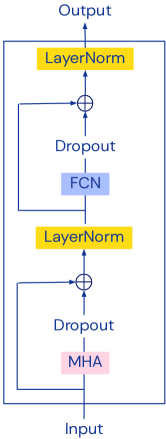
The standard use case of self-attention is with a skip connection inside the Transformer. A Transformer block is composed of residual blocks of multihead self-attention (MHA) and fully-connected (FCN) layers (Figure 1).
Hence similarly to invertible ResNets, we can normalise L2-MHA by the upper bounds given in Theorem 3.2 to obtain Contractive-L2-MHA , with which we can obtain invertible self-attention .
Since Dropout is also part of the residual branch along with Contractive-L2-MHA, we should check that it is also contractive.
At test time, Dropout multiplies inputs by the dropout keep probability , so it is a contraction with Lipschitz constant at evaluation time.
At training time, Dropout amounts to setting some inputs to zero, while keeping other inputs constant. This can be expressed as right multiplication by a diagonal binary matrix , and for such matrices we can verify .
Notice that LayerNorm is not part of the residual branch, hence its Lipschitz continuity is not relevant for invertibility; rather, we can replace it with an invertible normalisation such as ActNorm (Kingma & Dhariwal, 2018).
However, architectures that place LayerNorm inside the residual branch (termed pre-LN as opposed to the traditional post-LN in Figure 1) have become more prevalent in the literature (Wang et al., 2019; Xiong et al., 2020), and in this case it makes sense to investigate its Lipschitz continuity.
We show that LayerNorm is Lipschitz in Appendix N, with a bound on its Lipschitz constant.
In the next section, we investigate the properties of invertible self-attention and how it compares with the standard dot-product self-attention; we replace DP-MHA in the Transformer with Contractive-L2-MHA, hence replacing the residual self-attention module with invertible self-attention.
We are not interested in the modified Transformer per se, but rather in comparing the properties of invertible self-attention to standard self-attention — we only use the Transformer as a testbed for this purpose, since self-attention is commonly used in a Transformer.
Given the theoretical focus of the paper, we believe that a more challenging application of invertible self-attention, such as normalising flow-based modelling, would be more suitable as a separate paper focused on that particular application.
5 Experimental Results
5.1 Asymptotic tightness of the upper bound on
A tight bound on the Lipschitz constant of self-attention is desirable for all listed applications in Section 1; it leads to tighter generalisation bounds, lighter constraints for provable robustness, and better expressiveness in residual flow models.
Hence we investigate the tightness of our bound on the Lipschitz constant of L2-MHA.
The Lipschitz constant is a supremum over the space of inputs (c.f. Equation (2)) and approximating it requires solving an intractable
optimisation problem.
Hence it is infeasible to estimate accurately in general, especially when is high-dimensional.
However, we may compute a lower bound on the Lipschitz constant by maximising the norm of the Jacobian with respect to until convergence.
This local optimum will form a lower bound by Theorem 2.1, and we can expect this lower bound to be fairly tight for the low-dimensional case, provided the optimisation is thorough.
We use this observation to provide empirical evidence for the asymptotic tightness of the upper bound on in Theorem 3.2.
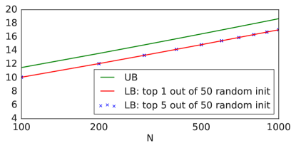
In Figure 2, we show the upper bound as well as the lower bound on obtained by optimising with respect to for L2-MHA with 50 different random initialisations of , with and varying between and .
See Appendix H for further details.
Note that we use a log-scale for the x-axis, and recall that the upper bound is , dominated by the term for large .
Hence the plot for the upper bound shows a linear trend.
We also observe that the slope of the lower bound is very similar, providing empirical evidence that the upper bound is asymptotically tight.
There are at least two possible explanations for the gap between the upper and lower bounds.
(1) The lower bound is only a local optimum — the true Lipschitz constant is a global optimum across inputs, which can be difficult to attain especially for high values of .
(2) The multiplicative constant of the upper bound may be loose.
Assuming asymptotic tightness, it remains an open question whether the multiplicative constant can be tightened.
We show the analogous plot for and discuss the results in Appendix J.
Additionally in Appendix K, we show that optimising w.r.t. for DP-MHA causes the norm to diverge, providing empirical verification of Theorem 3.1, that DP-MHA is indeed not Lipschitz.
5.2 Numerical invertibility of MHA residual map

Recall from Section 4.1 that is invertible if is contractive.
Hence if is Contractive-L2-MHA, is necessarily invertible.
However, technically we do not disprove the invertibility of DP-MHA, since the converse does not hold in general i.e. if is DP-MHA, which we have shown is not Lipschitz hence not contractive, it may still be the case that is invertible.
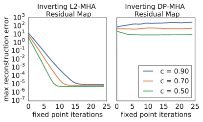
To verify that DP-MHA (with the skip connection) is not invertible in practice, we compare the numerical invertibility of the residual map between the cases where is L2-MHA and DP-MHA in Figure 3.
For each, we take MHA with heads and randomly initialised weights, and quantify the maximum reconstruction error across a batch of inputs whose outputs are inverted via the fixed-point iteration described in Section 4.1. We use ,
,
and
(see Appendix I for analogous results for a wider range of and and for DP-MHA with trained weights).
To highlight the difference between the two types
of self-attention, recall in the proof of Theorem 3.1 (showing that DP-MHA is not Lipschitz) that when one of the inputs is , some terms of the Jacobian grow with the sample variance of .
Hence we check numerical invertibility at a set of inputs where and are chosen uniformly at random.
In Figure 3, we see that DP-MHA is not invertible whereas L2-MHA is invertible for sufficiently small .
This shows how not having the theoretical guarantee of being contractive can cost us invertibility in practice.
We note that the figure shows local invertibility at the sampled inputs, as opposed to global invertibility across the whole input space, yet this clearly highlights the difference between the two choices of self-attention.
Experiments with the globally invertible self-attention obtained by normalising with the Lipschitz upper bound are provided in the next section.
5.3 Expressiveness of L2-MHA and invertible self-attention
A natural question to ask is: how does the expressiveness of L2-MHA and Contractive-L2-MHA (that leads to invertible self-attention with the skip connection) compare with the original DP-MHA?
We expect that the Lipschitz constraint will limit the expressiveness of the Transformer, and would like to find out by how much.
We investigate this by comparing the performance of the original Transformer and the Transformer with invertible self-attention (c.f. Figure 1) at character-level language modelling on the Penn Treebank dataset (Marcus et al., 1993).
We compare the test negative log-likelihood (NLL) of a baseline LSTM, the original Transformer (DP-MHA), and a series of models between the original Transformer and the Transformer with invertible self-attention (Contractive-L2-MHA),
making one change at a time and tuning the hyperparameters on a validation set.
For Contractive-L2-MHA, we normalise L2-MHA by the bound on as it is tighter than the bound on .
During training we backpropagate through these contractive blocks (including the denominator) to update the model parameters.
We found that only backpropagating through the numerator (i.e. applying stop-gradient to denominator) gave slightly worse performance.
See Appendix H for experimental details.
The results are shown in Figure 4.
The first plot shows the best performing LSTM reaching a test NLL of around , and the second plot shows the best performing Transformer reaching a slightly improved performance for – layers of Transformer blocks.
We observe instabilities in training for a higher number of layers, requiring careful tuning of the learning rate schedule for stability at the cost of performance, a commonly observed phenomenon in the literature of deep Transformer architectures (Bapna et al., 2018; Parisotto et al., 2020).
The third plot shows results for the Transformer with DP-MHA replaced with L2-MHA but without tying and , and we observe a very similar test performance.
The fourth plot shows the change when we further tie the query and key weights (making ); we see that there is a small degradation in performance.
Here the number of trainable parameters has been reduced, but in Appendix L we show that matching parameter count does not help performance, suggesting that the reduction in performance when tying queries and keys is not solely due to having fewer parameters.
We note that performance saturates at around layers for each Transformer model so far.
On the rightmost plot we show results when further dividing self-attention in each block by the upper bound on , to obtain invertible self-attention.
This does give reduced performance for the same number of layers, but we can attain similar performance with more layers, no longer saturating at layers.
| Number of Layers | 2 | 4 | 6 | 8 | 10 | 12 | 14 | 16 | 18 |
|---|---|---|---|---|---|---|---|---|---|
| Transformer (DP) | 1.061 | 1.032 | 1.021 | 1.017 | 1.025 | - | - | - | - |
| Transformer (L2), | 1.168 | 1.040 | 1.023 | 1.024 | 1.019 | 1.008 | 1.018 | 1.027 | 1.034 |
| Transformer (Contractive-L2) | 1.246 | 1.135 | 1.103 | 1.079 | 1.072 | 1.060 | 1.039 | 1.029 | 1.031 |
Thus we conclude the following. (1) Replacing the dot-product with the L2 distance incurs hardly any loss in expressiveness. (2) Tying the query and key weights to obtain Lipschitz self-attention incurs a small loss in expressiveness. (3) Dividing by the upper bound on to obtain invertible self-attention incurs a noticeable loss in expressiveness, but also has a stabilising effect on the optimisation of the Transformer, thus allowing one to compensate for the apparent loss in expressiveness by increasing the number of layers.
5.4 Training Stability of DP-MHA vs L2-MHA
In Figure 5, we compare the output variance of trained L2-MHA against trained DP-MHA, with weights from the one-layer Transformer (L2), model and (DP) model used for Figure 4 respectively. We take the same distribution of inputs as used for the numerical invertibility experiment in Section 5.2, and show the histogram of inputs and outputs after flattening the input/output tensors. We see that the range of outputs remains similar to the range of inputs for Lipschitz L2-MHA, whereas for DP-MHA the outputs have a much wider range, because the Jacobian norm is large for DP-MHA at these inputs.
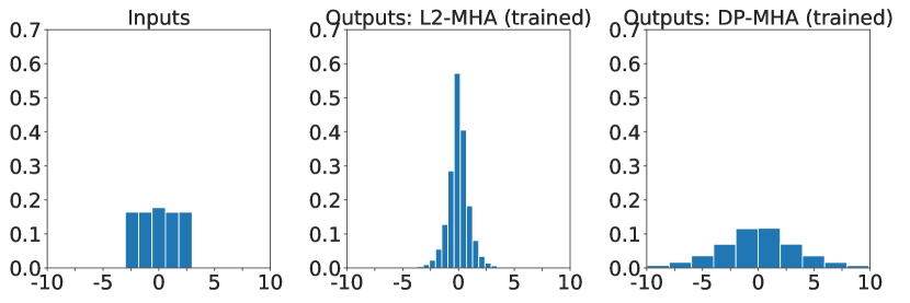
In practice, this leads to instabilities in training for DP-MHA, hence requiring careful tuning of the learning rate schedule for training deeper Transformer models: linear warmup and square root decay, as detailed in Appendix H.
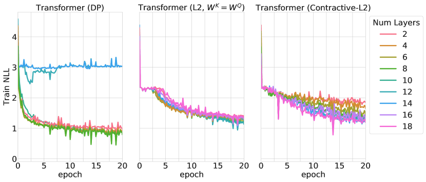
We investigate the behaviour of the different Transformer models on the above PTB task when using a fixed learning rate.
We observe that DP-MHA fails to train at all beyond 10 layers, whereas both L2-MHA () (i.e. Lipschitz L2-MHA but not contractive) and Contractive-L2-MHA shows stable training for up to 18 layers (see Appendix M for the training curves).
This was the deepest model we could fit on a single GPU, and we expect to be able to train even deeper models with these two.
In Table 1 we show the best Test NLL across training for each of the Transformer models. Note that for DP-MHA training becomes unstable beyond 10 layers, so we are only able to provide results up to 10 layers. The generalisation performance of the best model for each setting of self-attention is similar.
6 Conclusion and Discussion
We have shown that the widely used dot-product self-attention is not Lipschitz, and that the proposed L2 self-attention is Lipschitz, by deriving an Lipschitz bound for and an bound for , where is the input sequence length. We also provided empirical evidence of the asymptotic tightness of the bound for . We demonstrated that Lipschitz-constrained self-attention can be used to formulate invertible self-attention, which we experimentally evaluated on a character-level language modelling task. And finally, we also showed that L2-MHA is more stable during training, allowing the use of fixed learning rate for stable training of deep architectures.
Our approach to Lipschitz self-attention has been to replace the dot-product kernel with an L2 kernel. An alternative would be to constrain the inputs of self-attention to be bounded; if the input space is compact, e.g. , any continuously differentiable function is Lipschitz, including dot-product self-attention. However, while being simple to implement, this solution has its own difficulties. First, it makes the Lipschitz constant depend on the range of the input, and thus obtaining a tight bound would require non-trivial mathematical work. We stress that a guarantee that the function is Lipschitz does not tell us anything about its Lipschitz constant; without a tight Lipschitz bound, the true Lipschitz constant can be very large, at which point it is unhelpful that the function is Lipschitz. Second, since self-attention is typically applied at multiple layers within a model (e.g. Transformer), the input to each self-attention will live in a different compact set that depends on the parameters of the previous layers, complicating the analysis for subsequent layers. A solution is to constrain the inputs of each layer to be in the same compact set, e.g. by passing them through a sigmoid non-linearity. This however can have undesirable side effects such as vanishing gradients when the sigmoids are saturated. Despite these difficulties, this could be a worthwhile alternative route for obtaining Lipschitz self-attention to explore in the future.
Having a provably Lipschitz self-attention module at our disposal makes it possible to use Transformer-based architectures in applications requiring Lipschitz constraints, while enjoying theoretical guarantees. A natural application of Lipschitz self-attention is for residual flows (Behrmann et al., 2019), and for parameterising Neural ODEs (Chen et al., 2018) where a Lipschitz vector field guarantees the existence of a unique solution to the ODE for all times. These models can be used for density estimation and generative modelling of sets. Another interesting direction for future work would be to analyse different variants of self-attention based on kernels other than dot-product and L2, as (Tsai et al., 2019) do from an experimental perspective, for which we believe the mathematical tools developed in this paper may aid the analysis.
Acknowledgements
We would like to thank Adam Kosiorek, Arnaud Doucet, Yee Whye Teh, Michalis Titsias, Emilien Dupont and Theophane Weber for helpful discussion and feedback.
References
- Abadi et al. (2016) Abadi, M., Agarwal, A., Barham, P., Brevdo, E., Chen, Z., Citro, C., Corrado, G. S., Davis, A., Dean, J., Devin, M., et al. TensorFlow: Large-scale machine learning on heterogeneous distributed systems. arXiv preprint arXiv:1603.04467, 2016.
- Anil et al. (2019) Anil, C., Lucas, J., and Grosse, R. Sorting out Lipschitz function approximation. In International Conference on Machine Learning, pp. 291–301, 2019.
- Bapna et al. (2018) Bapna, A., Chen, M. X., Firat, O., Cao, Y., and Wu, Y. Training deeper neural machine translation models with transparent attention. In Proceedings of the 2018 Conference on Empirical Methods in Natural Language Processing, pp. 3028–3033, 2018.
- Behrmann et al. (2019) Behrmann, J., Grathwohl, W., Chen, R. T. Q., Duvenaud, D., and Jacobsen, J.-H. Invertible residual networks. In Proceedings of the 36th International Conference on Machine Learning, 2019.
- Brown et al. (2020) Brown, T. B., Mann, B., Ryder, N., Subbiah, M., Kaplan, J., Dhariwal, P., Neelakantan, A., Shyam, P., Sastry, G., Askell, A., et al. Language models are few-shot learners. arXiv preprint arXiv:2005.14165, 2020.
- Chen et al. (2018) Chen, R. T. Q., Rubanova, Y., Bettencourt, J., and Duvenaud, D. Neural ordinary differential equations. In Advances in Neural Information Processing Systems, pp. 6571–6583, 2018.
- Chen et al. (2019) Chen, R. T. Q., Behrmann, J., Duvenaud, D., and Jacobsen, J.-H. Residual flows for invertible generative modeling. In Advances in Neural Information Processing Systems, 2019.
- Cisse et al. (2017) Cisse, M., Bojanowski, P., Grave, E., Dauphin, Y., and Usunier, N. Parseval networks: Improving robustness to adversarial examples. In Proceedings of the 34th International Conference on Machine Learning, pp. 854–863, 2017.
- Corless et al. (1996) Corless, R. M., Gonnet, G. H., Hare, D. E., Jeffrey, D. J., and Knuth, D. E. On the Lambert W function. Advances in Computational mathematics, 5(1):329–359, 1996.
- Devlin et al. (2019) Devlin, J., Chang, M.-W., Lee, K., and Toutanova, K. BERT: Pre-training of deep bidirectional transformers for language understanding. In Proceedings of the 2019 Conference of the North American Chapter of the Association for Computational Linguistics, pp. 4171–4186, 2019.
- Fazlyab et al. (2019) Fazlyab, M., Robey, A., Hassani, H., Morari, M., and Pappas, G. Efficient and accurate estimation of Lipschitz constants for deep neural networks. In Advances in Neural Information Processing Systems, pp. 11423–11434, 2019.
- Federer (1969) Federer, H. Geometric Measure Theory. Classics in Mathematics. Springer Berlin Heidelberg, 1969. ISBN 9783642620102.
- Glorot & Bengio (2010) Glorot, X. and Bengio, Y. Understanding the difficulty of training deep feedforward neural networks. In Proceedings of the thirteenth international conference on artificial intelligence and statistics, pp. 249–256, 2010.
- Grathwohl et al. (2019) Grathwohl, W., Chen, R. T. Q., Betterncourt, J., Sutskever, I., and Duvenaud, D. FFJORD: Free-form continuous dynamics for scalable reversible generative models. In International Conference on Learning Representations, 2019.
- Huang et al. (2019) Huang, C.-Z. A., Vaswani, A., Uszkoreit, J., Simon, I., Hawthorne, C., Shazeer, N., Dai, A. M., Hoffman, M. D., Dinculescu, M., and Eck, D. Music Transformer. In International Conference on Learning Representations, 2019.
- Kingma & Ba (2015) Kingma, D. P. and Ba, J. Adam: A method for stochastic optimization. In 3rd International Conference on Learning Representations, 2015.
- Kingma & Dhariwal (2018) Kingma, D. P. and Dhariwal, P. Glow: Generative flow with invertible convolutions. In Advances in Neural Information Processing Systems, pp. 10215–10224, 2018.
- Latorre et al. (2020) Latorre, F., Rolland, P., and Cevher, V. Lipschitz constant estimation of neural networks via sparse polynomial optimization. In International Conference on Learning Representations, 2020.
- Marcus et al. (1993) Marcus, M. P., Marcinkiewicz, M. A., and Santorini, B. Building a large annotated corpus of English: The Penn Treebank. Computational Linguistics, 19(2):313–330, 1993.
- Mises & Pollaczek-Geiringer (1929) Mises, R. and Pollaczek-Geiringer, H. Praktische verfahren der gleichungsauflösung. ZAMM-Journal of Applied Mathematics and Mechanics/Zeitschrift für Angewandte Mathematik und Mechanik, 9(2):152–164, 1929.
- Miyato et al. (2018) Miyato, T., Kataoka, T., Koyama, M., and Yoshida, Y. Spectral normalization for Generative Adversarial Networks. In International Conference on Learning Representations, 2018.
- Parisotto et al. (2020) Parisotto, E., Song, H. F., Rae, J. W., Pascanu, R., Gulcehre, C., Jayakumar, S. M., Jaderberg, M., Kaufman, R. L., Clark, A., Noury, S., Botvinick, M. M., Heess, N., and Hadsell, R. Stabilizing Transformers for reinforcement learning. In International Conference on Machine Learning, 2020.
- Parmar et al. (2019) Parmar, N., Ramachandran, P., Vaswani, A., Bello, I., Levskaya, A., and Shlens, J. Stand-alone self-attention in vision models. In Advances in Neural Information Processing Systems, pp. 68–80, 2019.
- Peyré & Cuturi (2019) Peyré, G. and Cuturi, M. Computational optimal transport. Foundations and Trends in Machine Learning, 11(5-6):355–607, 2019.
- Sokolić et al. (2017) Sokolić, J., Giryes, R., Sapiro, G., and Rodrigues, M. R. Robust large margin deep neural networks. IEEE Transactions on Signal Processing, 65(16):4265–4280, 2017.
- Tsai et al. (2019) Tsai, Y.-H. H., Bai, S., Yamada, M., Morency, L.-P., and Salakhutdinov, R. Transformer dissection: An unified understanding for Transformer’s attention via the lens of kernel. In Proceedings of the 2019 Conference on Empirical Methods in Natural Language Processing and the 9th International Joint Conference on Natural Language Processing, pp. 4344–4353, 2019.
- Tsuzuku et al. (2018) Tsuzuku, Y., Sato, I., and Sugiyama, M. Lipschitz-margin training: Scalable certification of perturbation invariance for deep neural networks. In Advances in Neural Information Processing Systems, pp. 6541–6550, 2018.
- Vaswani et al. (2017) Vaswani, A., Shazeer, N., Parmar, N., Uszkoreit, J., Jones, L., Gomez, A. N., Kaiser, Ł., and Polosukhin, I. Attention is all you need. In Advances in Neural Information Processing Systems, pp. 5998–6008, 2017.
- Virmaux & Scaman (2018) Virmaux, A. and Scaman, K. Lipschitz regularity of deep neural networks: analysis and efficient estimation. In Advances in Neural Information Processing Systems, pp. 3835–3844, 2018.
- Vuckovic et al. (2020) Vuckovic, J., Baratin, A., and Tachet des Combes, R. A mathematical theory of attention. arXiv preprint arXiv:2007.02876, 2020.
- Wang et al. (2019) Wang, Q., Li, B., Xiao, T., Zhu, J., Li, C., Wong, D. F., and Chao, L. S. Learning deep transformer models for machine translation. In Proceedings of the 57th Annual Meeting of the Association for Computational Linguistics, pp. 1810–1822, 2019.
- Wang et al. (2018) Wang, X., Girshick, R., Gupta, A., and He, K. Non-local neural networks. In Proceedings of the IEEE Conference on Computer Vision and Pattern Recognition, pp. 7794–7803, 2018.
- Xiong et al. (2020) Xiong, R., Yang, Y., He, D., Zheng, K., Zheng, S., Xing, C., Zhang, H., Lan, Y., Wang, L., and Liu, T. On layer normalization in the transformer architecture. In International Conference on Machine Learning, pp. 10524–10533. PMLR, 2020.
- Zhang et al. (2019) Zhang, H., Goodfellow, I., Metaxas, D., and Odena, A. Self-attention Generative Adversarial Networks. In Proceedings of the 36th International Conference on Machine Learning, pp. 7354–7363, 2019.
Appendix
Appendix A Useful Identities for deriving Jacobian expressions
In this section, we list some useful identities for deriving the Jacobians of the expressions in the paper.
Suppose is a scalar, are column vectors, and is a vector valued function. We use the standard convention that for , , we have . Then we have the following chain rule identities:
-
•
-
•
-
•
Note is a row vector, so is a matrix.
The Jacobian of the softmax is also well-known. Suppose . Then
Appendix B Power Iteration
Although can be computed efficiently in time for , naïvely computing requires operations. (By we denote the greatest eigenvalue of a symmetric matrix .) We can however obtain an underestimate via power iteration:
| (9) |
with each iteration taking time. Then using iterations gives us an underestimate in time. Since this is an underestimate, the resulting approximation to the Lipschitz constant of the linear map will not be an upper bound. However the number of power iterations is usually chosen so that is accurate enough — is shown to be sufficient in the context of fully connected networks or convolutions considered by Behrmann et al. (2019).
The iteration will converge if has an eigenvalue that is strictly greater in magnitude than its other eigenvalues, and the starting vector has a nonzero component in the direction of an eigenvector associated with the dominant eigenvalue. This happens with probability if is chosen at random, and the convergence is geometric with ratio where is the eigenvalue with second largest magnitude (Mises & Pollaczek-Geiringer, 1929).
Appendix C Proof of Theorem 3.1 for General
Theorem 3.1.
DP-MHA is not Lipschitz for any vector -norm with .
Proof.
The mapping can be written as
| (10) |
where and with . Hence can be interpreted as a map of each to a point in the convex hull of . Since is a map from to , its Jacobian is
| (11) |
where . By taking partial derivatives we can show that where is a binary matrix with zeros everywhere except the th entry, is the Kronecker delta, and . So for :
| (12) |
For the last equality, note has all rows equal to zero except for the th row given by . We can then verify that simplifies to .
For vector -norms, is bounded if and only if its entries are bounded, by definition of the operator norm. The entries of are bounded for arbitrary only if the entries of are bounded. So let us investigate the entries of this matrix. Writing out each term of the matrix, we observe that it is in fact a covariance matrix of a discrete distribution. Specifically:
| (13) |
where is a discrete distribution with support at the inputs and probability mass function given by their softmax probabilities . A consequence of this interpretation is that is positive semi-definite (PSD) since for , Equation (13) becomes , with equality if and only if the are all equal.
We use this observation to show that the terms of are unbounded, and so DP-MHA is not Lipschitz.
Consider the case . Then , i.e. we have uniform attention regardless of .
The first term of in Equation (12) disappears since , and the last term becomes . For the second term, the entries are unbounded since the latter is equal to the sample variance of , which can be arbitrarily large.
Note that we have shown that single head dot-product self-atttention () is not Lipschitz, but it is clear that this implies multihead self-attention DP-MHA is also not Lipschitz, since the output of multihead attention is a linear combination of the outputs of each head.
∎
Appendix D Bias term in DP Self-Attention
A natural question to ask is whether we can add bias terms to and to to resolve the issue of attention weights becoming uniform when . The answer is no in general. It can again be shown that is unbounded when is chosen such that (such a choice is possible assuming is full rank, a dense set in ). Then again, and the diagonal entries of are unbounded.
Appendix E Efficient Computation of L2 Self-Attention
Dot-product self-attention only requires a few matrix multiplications to compute the logits (i.e. the inputs to the softmax) between all pairs of inputs, without having to loop over pairs, hence it can be computed efficiently. Similarly, we can show that L2 self-attention can also be computed in an efficient manner. Using the identity we can compute the logits of L2 attention between all pairs via matrix multiplications and computation of row-wise L2 norms, with negligible overhead compared to dot-product self-attention. Specifically, for L2 self-attention we can show that
| (14) |
where applies the squared L2 norm to each row of , so if then .
In Table 2 we show the wall-clock training times for the Transformer models with different attention functions and a varying number of layers. It is evident that the differences between the models are rather small.
| 1 Layer | 2 Layers | 3 Layers | 4 Layers | 5 Layers | |
|---|---|---|---|---|---|
| Transformer (DP) | 37 | 56 | 77 | 92 | 110 |
| Transformer (L2) | 35 | 56 | 73 | 99 | 115 |
| Transformer, (L2) | 39 | 58 | 79 | 91 | 108 |
| Transformer, (Contractive-L2) | 37 | 60 | 81 | 102 | 127 |
Appendix F Proof of Theorem 3.2
Recall the formulation of L2-MHA:
where we have that , , and , and the softmax is applied to each row of the input matrix. Recall Equation (14):
F.1 L2 self-attention is not Lipschitz for general
Let us first look at the case of and suppress the index to reduce clutter. Consider the map , so . We need to be Lipschitz for and hence to be Lipschitz. Note that is defined as:
and the normalisation constant satisfies , for , .
For L2 self-attention, we may take partial derivatives and use the chain rule to show that the Jacobian of is:
| (15) |
with
| (16) |
where
| (17) |
and
Recall that is a binary matrix with zeros everywhere except the th entry. Hence has all rows equal to zero except for the th row given by . We can then verify:
| (18) |
Also note is symmetric, and each row/colum sums to , i.e. . Hence we may simplify the Jacobian terms as follows:
| (19) |
and for :
| (20) |
We are now ready to show that is not Lipschitz for general :
Lemma F.1.
If is full rank (i.e. full column rank), and , then has terms that are unbounded for , hence is not Lipschitz.
Proof.
Let us investigate the expression for , which is related to as follows by Equation (20):
It suffices to show that is unbounded to show that is unbounded, since is full rank and .
Let . Then we have:
Hence . Note can take an arbitrary value in , since and is full-rank.
For all , let us choose such that . This is possible for any value of since is full-rank. Note and not . We then have that is equal for all , hence for all . Then for , simplifies to
whose entries are unbounded since can be any vector in (note we assume for self-attention to be well-defined, hence ). ∎
The intuition for this result is as follows: a reason for DP-MHA not being Lipschitz is that for ,, the attention weights become uniform regardless of the values of for . A similar issue arises for L2-MHA with and full-rank , as shown above: given any , we can choose such that the become uniform.
F.2 L2 self-attention is Lipschitz for
Hence we impose the restriction that . With this assumption we have
| (21) |
where and is chosen such that , in particular . The terms in the Jacobian of simplify to:
| (22) | ||||
| (23) |
Let the Jacobian of be:
| (24) |
Since , and by the chain rule (by symmetry of ), we have that . Hence
| (25) | ||||
| (26) |
Noting , we would like to upper bound .
F.2.1 Upper bound on for L2-MHA
Consider the choice , where is the maximum absolute row sum of . A key observation is that if we can bound the -norm of the Jacobian of , a single output of , (i.e. a single block row of ) then this is also a bound on due to permutation equivariance of self-attention; all block rows have the same maximal when each is optimised over the input . Using this, we can prove that admits an upper bound that is . Below we state and prove lemmas that lead to the proof of this upper bound.
First we analyse the term , that appears in the first term of . Note that for , so that the rows of are , we have
| (27) |
where . The last equality uses the observation in Equation (7).
The central inequality used throughout the proof of the main theorem is the following:
Lemma F.2.
where is a one-dimensional invertible function on .
Proof.
The first equality holds since . The next inequality holds since where . The final inequality can be proved as follows.
We would like to bound
| (28) |
where (hence ). Define:
| (29) |
First note that as , exponentially fast, causing the product . Hence we expect the above quantity to be bounded and attain its maximum.
Let for notational conciseness, and note . By taking partial derivatives with the chain rule, we have that for
| (30) |
Hence the derivative is if and only if or , the latter being equivalent to . Hence at the maximum, the non-zero values among must be equal to one another. It is clear now that the maximum value is attained when for (and recall ). So for . Substituting this into , and rearranging, we obtain . Note is increasing for hence . ∎
Note for . Since is increasing, we have for . In fact, it is known that (Corless et al., 1996).
Note the term in allows us to use the above inequality, since now appears in the terms of :
| (31) | ||||
| (32) |
Using the inequalities , and , we have:
For the first equality, note that . For the second equality, note that the summand for is because the term . Each of the terms in the brackets are bounded by the following lemmas:
Lemma F.3.
( defined as in Lemma F.2).
Proof.
Recall that . Let denote the standard deviation of . Then . Hence
since (by e.g. using the Cauchy–Schwartz inequality on and ) and , and the last inequality is from Lemma F.2. ∎
Lemma F.4.
.
Proof.
Note for real vectors . Hence
where , .
Note since for vector . Hence .
Also since for (e.g. by the Cauchy–Schwartz inequality on and ). Hence .
Putting the above lemmas altogether, with the observation by permutation invariance of (since is permutation equivariant and is the maximum absolute row sum), we have
| (33) | ||||
where the last inequality holds for .
The full multihead attention map that combines the heads is:
where , and
Note the Jacobian is a block matrix whose rows are , hence , and similarly . Hence we have
Combining this with Inequality (33), we have:
F.2.2 Upper bound on for L2-MHA
For , we use the following lemma:
Lemma F.5.
Let A be a block matrix with block rows . Then , and equality holds if and only if the first right singular vectors of the align.
Proof.
Note that equality holds if and only if the first right singular vectors of the align. ∎
Hence a bound on the spectral norm of each block row of can give us an bound on , which may be loose, and it remains an open question as to whether this bound can be tightened.
To bound the norm of each row of , we use the following lemmas:
Lemma F.6.
Proof.
, where the first equality holds by symmetry of and the next holds by being positive semi-definite, so all its eigenvalues are non-negative, and hence the maximal eigenvalue is bounded by the sum of the eigenvalues, equal to its trace. The final inequality is from Lemma F.2. ∎
Lemma F.7.
Proof.
Directly use Cauchy–Schwartz on and in the proof of Lemma F.4. ∎
Again using the inequalities , and , with the additional equality , we have the bound:
Using Lemma F.5, we have that
| (34) | ||||
To obtain the final result for the full multihead self-attention , we need a final lemma:
Lemma F.8.
Let A be a block matrix with block columns . Then .
Proof.
where we are using the substitution , and the last inequality holds by e.g. Cauchy–Schwartz inequality on and . ∎
Appendix G The Case with Masking
Since self-attention is often used with masking, a natural question is how masking affects the derived bounds. In self-attention (for any choice of attention function), masking is implemented as follows: given a set of mask indices , the logits (i.e. the inputs to the softmax) are set to at the mask indices. That is,
where is the original logit (e.g. for L2 self-attention, ).
Masking implies is not a function of for , hence for . Thus is equal to the th output for self-attention with inputs restricted to , the unmasked inputs with respect to the th output. Hence will no longer contribute to the bound on , and hence the bound for the unmasked case will continue to hold as long as i.e. attends to itself (this is necessary for the proof of Lemma F.2 to hold). The bound can in fact be tightened by replacing with , the number of unmasked inputs with respect to the th output.
Appendix H Experimental Details
For the experiment in Section 5.1, showing the asymptotic tightness of the upper bound on where is L2-MHA, we fix all free parameters of (namely ) to be the identity, and only optimise the input .
We use random initialisations of for each , where for (we observed that having itself be random improves optimisation). We display the top results for each value of after optimising each random initialisation till convergence using Adam (Kingma & Ba, 2015) with a learning rate of .
For the experiments in Section 5.3, we comparing the performance of the original Transformer and the Transformer with Lipschitz/invertible self-attention at character-level language modelling on the Penn Treebank dataset (Marcus et al., 1993).111We use the standard training-validation-test split, and the dataset can be found at e.g. https://github.com/harvardnlp/TextFlow/tree/master/data/ptb. Each training example is a sentence represented as a variable-length sequence of characters, and examples are batched according to length such that padding is minimised, with the maximum sequence length set to . All models are autoregressive, outputting the logits for the categorical likelihood predicting the next character, and are trained using maximum likelihood (cross-entropy loss) with a batch size of . The LSTM models have the dimensionality of the hidden state equal to the dimensionality of the cell state (the usual default implementation). The Transformer models are trained with a varying number of blocks (number of layers) with heads and , tuning hyperparameters for dropout rate in and base learning rate with number of warmup iterations for the standard custom learning rate schedule in Vaswani et al. (2017):
where is the learning rate at training iteration . Hence the learning rate linearly increases from to over iterations, then decays proportionally to .
We use Glorot Uniform initialisation (Glorot & Bengio, 2010) for all weights (), except for weights in L2-MHA that are initialised from , and is a hyperparameter. For , we used . All experiments were done in Tensorflow 1.14 (Abadi et al., 2016) on single Nvidia Tesla V100 GPUs.
Appendix I Numerical Invertibility of MHA Residual Map
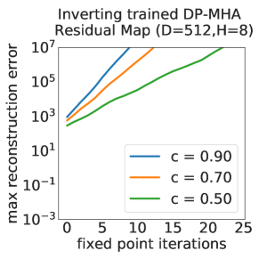
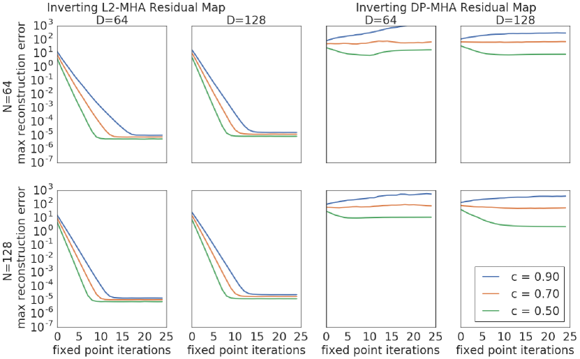
Following Section 5.2, Figure 6 confirms that numerical invertibility does not hold for trained weights for dot-product multihead self-attention (DP-MHA) (obtained from one-layer Transformer (DP) model used for Figure 4), similar to the randomly initialised weight case. Figure 7 shows additional results for different values of and .
Appendix J Behaviour of Lower Bound on
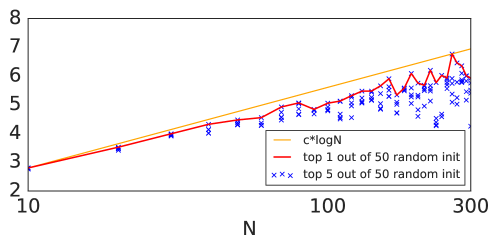
In Figure 8, we show the lower bound on obtained by optimising using the same optimisation procedure as for Figure 2 of Section 5.1. Here the optimisation is more difficult, evident in the variance of the top values, and the trend is less clear, but it appears that grows at a rate of . The message is less clear here, and there are at least two possibilities:
Appendix K Optimising the norm of the Jacobian of DP-MHA
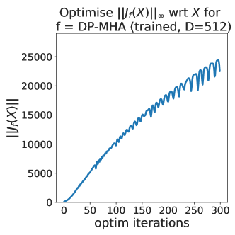
In Figure 9, we show how the norm of the Jacobian for DP-MHA keeps increasing when being optimised with respect to . This is a useful sanity check validating our theoretical result of Theorem 3.1, that DP-MHA is not Lipshchitz. The oscillations are likely due to momentum term of Adam optimizer that was used to optimise the norm.
Appendix L Experiment tying keys and queries of L2-MHA but preserving parameter count
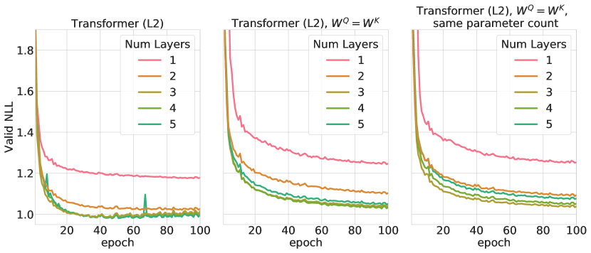
In Figure 4 of Section 5.3, we have shown that there is a clear reduction in performance when tying the keys and queries. To test whether this can be attributed to the reduction in parameter count, we tried doubling the number of columns of when the keys and queries are shared (i.e. from to ) so that the shared model has the same number of parameters as the unshared model. In Figure 10, the third column shows results for shared L2-MHA, but with the same number of parameters as the unshared L2-MHA i.e. without tying the keys and queries. The performance is similar to the second column (tying with a reduced number of parameters), suggesting that there is an inherent limitation in expressiveness to tying the keys and queries, and that the reduction in number of parameters is an insufficient explanation this phenomenon.
Appendix M Training curves for fixed learning rate DP-MHA vs L2-MHA
Appendix N The Lipschitz constant of LayerNorm
In this section, we show that LayerNorm is Lipschitz, with a loose bound on its Lipschitz constant w.r.t. to the -norm.
LayerNorm is defined as follows:
where . We will omit dependence on to write in cases when there is no ambiguity to reduce clutter.
In the trivial case where are all equal or when , hence , so its Lipschitz constant is 0. Thus let us assume and not all are equal.
First let us compute the derivative of and w.r.t :
where is a one-hot vector with at the th element. Note the penultimate equality holds because .
Now the derivative of , the th element of , w.r.t. is
Hence
Note
hence
| (36) |
recalling that is the maximum absolute row sum.
Let . Hence , and
Hence
Noting that this expression is scale-invariant in , we may assume WLOG , since we are assuming not all are equal and hence at least one is non-zero.
The expression now becomes
| (37) |
Since all terms are bounded, this continuous expression reaches a global maximum for some value of with .
It is easy to see that at the global maximum, : suppose this were to be true, WLOG . Then let us see how the quantity (37) changes when is increased by and is decreased by , keeping the sum constant. It is easy to see that the numerator stays constant, but the denominator changes by . Since for small , the numerator of (37) stays constant but the denominator decreases, the quantity (37) increases, contradicting that the global max is obtained for . Hence we may assume that .
Hence the quantity (37) (in particular, ) is differentiable at the global maximum, at which the partial derivatives of the following Lagrangian are zero:
From now on let us write for below to reduce clutter. Setting and noting , we obtain
Hence at the global maximum, takes one of two values and . Further we have that
| (38) |
If both and are among the , we have that . Solving for and plugging it in back to Equation (38), we get:
Since , and , is minimised when only one of the is and the rest are . Hence a crude lower bound on is , giving a bound:
| (39) |
However we conjecture that the true global maximum is attained when (i.e. all the for are equal to ), for which it is easy to show that .
Putting together the above, we have: