Characterization of Cooperators in Quorum Sensing with 2D Molecular Signal Analysis

Yuting Fang, Adam Noel, Andrew W. Eckford, Nan Yang, and Jing Guo This work was presented in part at IEEE Globecom 2019 [1].
Abstract

In quorum sensing (QS), bacteria exchange molecular signals to work together. An analytically-tractable model is presented for characterizing QS signal propagation within a population of bacteria and the number of responsive cooperative bacteria (i.e., cooperators) in a two-dimensional (2D) environment. Unlike prior works with a deterministic topology and a simplified molecular propagation channel, this work considers continuous emission, diffusion, degradation, and reception among randomly-distributed bacteria. Using stochastic geometry, the 2D channel response and the corresponding probability of cooperation at a bacterium are derived. Based on this probability, new expressions are derived for the moment generating function and different orders of moments of the number of cooperators. The analytical results agree with the simulation results obtained by a particle-based method. In addition, the Poisson and Gaussian distributions are compared to approximate the distribution of the number of cooperators and the Poisson distribution provides the best overall approximation. The derived channel response can be generally applied to any molecular communication model where single or multiple transmitters continuously release molecules into a 2D environment. The derived statistics of the number of cooperators can be used to predict and control the QS process, e.g., predicting and decreasing the likelihood of biofilm formation.

Index Terms:
Quorum sensing, molecular communication, 2D channel response, cooperative bacteria

I Introduction

Quorum sensing (QS) is a ubiquitous approach for microbial communities to respond to a variety of situations in which monitoring the local population density is beneficial. When bacteria use QS, they assess the number of other bacteria they can interact with by releasing and recapturing a molecular signal in their environment. This is due to the fact that a higher density of bacteria leads to more molecules that can be detected before they diffuse away or become degraded. If the number of molecules detected exceeds a threshold, then bacteria express target genes for a cooperative response. QS enables coordination within large groups of cells, potentially increasing the efficiency of processes that require a large population of cells working together. Microscopic populations utilize QS to complete many collaborative activities, such as virulence, bioluminescene, biofilms, and the production of antibiotics. These tasks play a crucial role in bacterial infections, environmental remediation, and wastewater treatment [2]. Since the QS process is highly dependent on signaling molecules, an accurate characterization of release, diffusion, degradation, and reception of such molecules across the environment in which bacteria live is very important to understand and control QS, which can help us to prevent undesirable bacterial infections and lead to new environmental remediation methods [3].

There are growing research efforts to study the coordination of bacteria via QS. Among them, [3, 4, 5] investigated the cooperative behavior of bacteria using simulation or biological experiments and [6, 7, 8, 9, 10, 11] mathematically modeled bacterial behavior coordination. We note that [6, 7, 8, 9, 10, 11] relied on abstract or simplifying models to represent the molecular diffusion channel (e.g., they did not consider the motion of individual signaling molecules based on Fick’s laws) in order to focus on understanding how behavior evolves over time. [12] considered a molecular diffusion channel between two clusters of bacteria, but did not consider the bacteria behavioral response. To the best of our knowledge, analyzing the statistics of the number of cooperative bacteria, taking into account the chemical reaction and diffusion of each molecule based on reaction-diffusion dynamics, is not available in the literature.

To control cooperative bacterial activities (e.g., biofilm formation and bioluminescene) for medical treatment and environmental monitoring, an analytically-tractable model needs to be developed since it predicts the cooperative behavior of bacteria, considering their noisy molecular signal propagation. We achieve this goal in this paper by leveraging the knowledge of QS, mass diffusion, stochastic geometry, and probability processes. Since our model accounts for the random motion of molecules based on reaction-diffusion equations, our model can be used to predict and control the impact of environment parameters, e.g., diffusion coefficient, reaction rate, and population density, on the concentration of molecules observed by bacteria and the statistics of the number of responsive cooperative bacteria.

In this paper, we consider a two-dimensional (2D) environment over which the bacteria are randomly spatially distributed according to a point process model. This is motivated by that bacteria may move in realistic environments and their locations may be not fixed. In the point process model, the locations of bacteria are changing between realizations [13, 14]. This means that the number of cooperative bacteria can change from one realization to the next. As a result, we are interested in the average result or distribution of the number of cooperative bacteria over a large number of realizations. We consider a 2D environment since a 2D environment facilitates future experimental validation of our current theoretical work. Biological experiments, especially with bacteria, are usually conducted in a 2D environment, e.g., bacteria residing on a petri dish (i.e., a thin plate for cell-culture) and the formation of biofilms [15]. While considering the topological randomness of bacteria, our model captures the basic features of QS by adopting the assumptions as follows: We assume that each bacterium acts as both a point transmitter (TX) and a circular receiver (RX), which captures the features of emission and reception of QS molecules. Since bacteria emit molecules sporadically in reality, we assume that each bacterium continuously111Note that continuous emission does not mean there is no time interval between two successive emissions of molecules. emits molecules at random times.

We emphasize that developing the analytical model in this paper is theoretically challenging since we need to address the random received signal at bacteria in random locations due to randomness in the motion and degradation of molecules, and randomness in the locations of many TXs. Despite these challenges, we make the following theoretical contributions:

  1. 1.

    We analytically derive the channel response (i.e., the expected number of molecules observed) at a RX due to continuous emission or an impulse emission of molecules at one point TX. Based on this, we then derive the channel response at a RX due to continuous emission of molecules from point TXs randomly distributed over a circle in a 2D environment.

  2. 2.

    Using the results in 1), we first derive the exact expression for the expected probability of cooperation at the bacterium at a fixed location, due to the emission of molecules from randomly-distributed bacteria, by using the Laplace transform of the random aggregate of received molecules. We then derive an approximate expression for such a probability, which is easier to compute than the exact expression, yet from our numerical results has good accuracy when the population density is sufficiently high.

  3. 3.

    Based on the results in 2), we derive approximate expressions for the moment generating function (MGF) and cumulant generating function (CGF) of the number of cooperative bacteria (i.e., cooperators). Using the MGF and the CGF, we derive approximate expressions for the n𝑛nth moment and cumulant of the number of cooperators. We study the convergence of the number of cooperators to a Gaussian distribution via the higher order statistics. We use the Poisson and Gaussian distributions with the derived statistics to analytically fit the probability mass function (PMF) and cumulative distribution function (CDF) of the number of cooperators. We show that the Poisson distribution provides the best overall approximation, based on our numerical results. In addition, we derive the expected number of pairs of two nearest bacteria both cooperating, which can be used to predict clusters of cooperators in a QS system.

We validate the accuracy of our analytical results via a particle-based simulation method where we track the random walk of each signaling molecule over time. In contrast to our preliminary work in [1], which only derives a portion of the results in 1) and the expected number of cooperators, this paper conducts a more comprehensive analysis of the 2D channel response, derives an exact expression for the expected probability of cooperation, and studies the distribution of the number of cooperators by its MGF and different order statistics.

Our derived statistical moments can help predict and control the QS process. For example, biofilm formation via QS is a mechanism for bacteria to resist antibiotics. However, a biofilm could be prevented from forming if the density of cooperators is too small. Our expressions reveal the impact of environmental factors (e.g., degradation and diffusion rates) on the likelihood of a given number of bacteria choosing to cooperate. Based on our expressions, we could infer how to decrease the likelihood of successful biofilm formation by adjusting environmental parameters. This could help optimize the performance of antibiotic treatment.

While contributing to QS, our results could also be applied to other molecular communication (MC) systems. More specifically, the 2D channel response could be used to determine the expected molecular signal observed at an RX when a TX (or TXs) impulsively or continuously releases molecules into a 2D environment in an MC system. The cooperating probability and statistical moments of the number of cooperators can be applied to study the group behavior of an MC system that uses consensus algorithms and broadcast channel models. For example, a cluster of nanomachines in a nanonetwork could secrete and sense molecules to achieve global network synchronization as proposed in [16]. Our derived cooperating probability and the number of cooperators could be used to determine the probability of a nanomachine being synchronized and the percentage of synchronized nanomachines in the nanonetwork.

We use the following notations: |x|𝑥|\vec{x}| denotes Euclidean norm of a vector x𝑥\vec{x}. N¯¯𝑁\overline{N} denotes the mean of a random variable (RV) N𝑁N and 𝔼Φ{}subscript𝔼Φ{\operatorname*{\mathbb{E}}}_{\Phi}\{\cdot\} denotes the expectation over a spatial random point process ΦΦ\Phi. Kn()subscript𝐾𝑛K_{n}(\cdot) denotes modified n𝑛nth order Bessel function of the second kind. In()subscript𝐼𝑛I_{n}(\cdot) denotes the modified n𝑛nth order Bessel function of the first kind [17]. Γ(a,z)Γ𝑎𝑧\Gamma(a,z) denotes the incomplete gamma function.

II System Model
Refer to caption
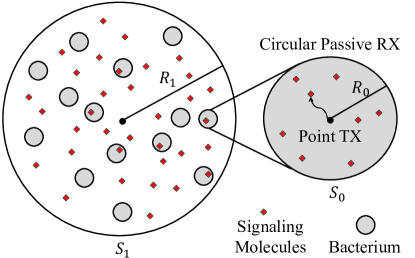
Figure 1: A population of bacteria randomly distributed over a circle S1subscript𝑆1S_{1} according to a 2D spatial point process, where each bacterium acts as a point TX and as a circular passive RX S0subscript𝑆0S_{0}. The molecules diffuse into and out of the bacteria.

We consider an unbounded 2D environment. Unlike a deterministic topology model, we consider a point process model to represent topological randomness of bacteria. There are several types of point processes and we consider the Poisson point process (PPP) in this paper[18] due to its tractable properties and well-known theorems. A population of bacteria is spatially distributed over a bounded circle S1subscript𝑆1S_{1} with radius R1subscript𝑅1R_{1} centered at (0,0)00(0,0) according to a 2D PPP with constant density λ𝜆\lambda, as shown in Fig. 1. We denote xisubscript𝑥𝑖\vec{x_{i}} as the location of the center of the bacterium i𝑖i where the bacterium i𝑖i is an arbitrary bacterium in the bacterial population. We denote Φ(λ)Φ𝜆\Phi\left(\lambda\right) as the set of random bacteria locations. We consider bacteria behavior analogous to QS, i.e., 1) emit signaling molecules; 2) detect the concentration of signaling molecules; and 3) decide to cooperate if the concentration exceeds a threshold. In the following, we detail the emission, propagation, and reception of signaling molecules, and the decision-making by the bacteria.

Emission: We consider that bacterium i𝑖i continuously releases molecules at different times, as shown in Fig. 3. The release time instants constitute points in a one-dimensional (1D) PPP and one molecule is released at each release time instant. We assume that the continuous emission of each bacterium follows an independent PPP with a rate q𝑞q. The rate q𝑞q is the average number of release time events within a unit time (i.e., 1 second). The rate q𝑞q is also equal to the number of molecules being released per second since one molecule is released at each release time event. We note that [19] and [20] also model molecules being emitted continuously at random times according to a 1D PPP.

Propagation: All A𝐴A molecules diffuse independently with a constant diffusion coefficient D𝐷D and they can degrade into a form that cannot be detected by the bacteria, i.e., A𝑘𝐴𝑘A\overset{k}{\rightarrow}\emptyset, where k𝑘k is the reaction rate constant in s1superscripts1\textnormal{s}^{-1}. If k=0𝑘0k=0, this degradation is negligible. Since we consider a single type of molecule, we only mention “the molecules”, i.e., omitting “A𝐴A”, in the remainder of this paper.

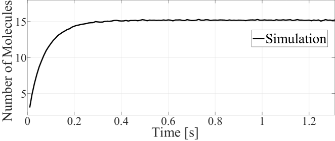
Reception: We model the bacterium i𝑖i as a circular passive RX with radius R0subscript𝑅0R_{0} and area S0subscript𝑆0S_{0} centered at xisubscript𝑥𝑖\vec{x_{i}}. The bacterium i𝑖i samples the number of molecules within S0subscript𝑆0S_{0} at only only one time instant t𝑡t. Bacteria perfectly count molecules if they are within S0subscript𝑆0S_{0}. Since the molecules released from all bacteria may be observed by the bacterium i𝑖i, the number of molecules observed at the bacterium i𝑖i at time t𝑡t, Nagg(xi,t|λ)superscriptsubscript𝑁aggsubscript𝑥𝑖conditional𝑡𝜆{N}_{\textnormal{agg}}^{{\dagger}}\left(\vec{x_{i}},t|\lambda\right), is given by Nagg(xi,t|λ)=xjΦ(λ)N(xi,t|xj)superscriptsubscript𝑁aggsubscript𝑥𝑖conditional𝑡𝜆subscriptsubscript𝑥𝑗Φ𝜆𝑁subscript𝑥𝑖conditional𝑡subscript𝑥𝑗N_{\textnormal{agg}}^{{\dagger}}\left(\vec{x_{i}},t|\lambda\right)=\sum_{\vec{x_{j}}\in\Phi\left(\lambda\right)}N\left(\vec{x_{i}},t|\vec{x_{j}}\right), where N(xi,t|xj)𝑁subscript𝑥𝑖conditional𝑡subscript𝑥𝑗N\left(\vec{x_{i}},t|\vec{x_{j}}\right) is the number of molecules observed at time at the bacterium i𝑖i due to the bacterium j𝑗j. The means of Nagg(xi,t|λ)superscriptsubscript𝑁aggsubscript𝑥𝑖conditional𝑡𝜆N_{\textnormal{agg}}^{{\dagger}}\left(\vec{x_{i}},t|\lambda\right) and N(xi,t|xj)𝑁subscript𝑥𝑖conditional𝑡subscript𝑥𝑗N\left(\vec{x_{i}},t|\vec{x_{j}}\right) are denoted by N¯agg(xi,t|λ)superscriptsubscript¯𝑁aggsubscript𝑥𝑖conditional𝑡𝜆\overline{N}_{\textnormal{agg}}^{{\dagger}}\left(\vec{x_{i}},t|\lambda\right) and N¯(xi,t|xj)¯𝑁subscript𝑥𝑖conditional𝑡subscript𝑥𝑗\overline{N}\left(\vec{x_{i}},t|\vec{x_{j}}\right), respectively. We assume that the expected number of molecules observed at the bacterium i𝑖i is constant after some time when degradation occurs. To demonstrate the suitability of this assumption, see Fig. 3 (and an analytical proof in Remark 1). In Fig. 3, N¯agg(xi,t|λ)superscriptsubscript¯𝑁aggsubscript𝑥𝑖conditional𝑡𝜆\overline{N}_{\textnormal{agg}}^{{\dagger}}\left(\vec{x_{i}},t|\lambda\right) is independent of t𝑡t after time t0.5s𝑡0.5st\approx 0.5\,\textnormal{s}. We denote time tisubscriptsuperscript𝑡𝑖t^{\star}_{i} as the time after which N¯agg(xi,t|λ)superscriptsubscript¯𝑁aggsubscript𝑥𝑖conditional𝑡𝜆\overline{N}_{\textnormal{agg}}^{{\dagger}}\left(\vec{x_{i}},t|\lambda\right) is approximately constant, i.e.,

N¯agg(xi,t|λ)|t>tilimtN¯agg(xi,t|λ)=N¯agg(xi,|λ).evaluated-atsuperscriptsubscript¯𝑁aggsubscript𝑥𝑖conditional𝑡𝜆𝑡subscriptsuperscript𝑡𝑖subscript𝑡superscriptsubscript¯𝑁aggsubscript𝑥𝑖conditional𝑡𝜆superscriptsubscript¯𝑁aggsubscript𝑥𝑖conditional𝜆\displaystyle\overline{N}_{\textnormal{agg}}^{{\dagger}}\!\left(\vec{x_{i}},t|\lambda\right)\!|_{t>t^{\star}_{i}}\!\approx\!\lim_{t\rightarrow\infty}\!\overline{N}_{\textnormal{agg}}^{{\dagger}}\!\left(\vec{x_{i}},t|\lambda\right)\!=\!\overline{N}_{\textnormal{agg}}^{{\dagger}}\!\left(\vec{x_{i}},\infty|\lambda\right). (1)

We also refer to any observation after tisubscriptsuperscript𝑡𝑖t^{\star}_{i}, i.e., N¯agg(xi,|λ)superscriptsubscript¯𝑁aggsubscript𝑥𝑖conditional𝜆\overline{N}_{\textnormal{agg}}^{{\dagger}}\!\left(\vec{x_{i}},\infty|\lambda\right), as an asymptotic observation. Notably, similar steady observations at the asymptotic stage have also been shown in [19] and [20].

Refer to caption
Figure 2: An example of release times due to continuous emission of molecules at a bacterium according to a random process.
Refer to caption
Figure 3: The average number of molecules observed at time t𝑡t, N¯agg(xi,t|λ)superscriptsubscript¯𝑁aggsubscript𝑥𝑖conditional𝑡𝜆\overline{N}_{\textnormal{agg}}^{{\dagger}}\left(\vec{x_{i}},t|\lambda\right), versus time t𝑡t. R1=20μmsubscript𝑅120𝜇mR_{1}=20\,{\mu}\textnormal{m}, λ=7.9×10²/μm2𝜆7.9superscript102𝜇superscriptm2\lambda=7.9\times 10^{-2}/{\mu}\textnormal{m}^{2}, xi=(10μm,10μm)subscript𝑥𝑖10𝜇m10𝜇m\vec{x_{i}}=(10\,{\mu}\textnormal{m},10\,{\mu}\textnormal{m}); see other simulation details in Sec. VI.

Decision-Making: We assume that the bacterium i𝑖i uses its asymptotic observation to make a decision, when the expected number of observed molecules becomes stable. This assumption is reasonable since tisubscriptsuperscript𝑡𝑖t^{\star}_{i} is very small, e.g., t=0.5s𝑡0.5st=0.5\,\textnormal{s} in Fig. 3, and bacteria can reach the steady state very quickly, especially relative to the timescale of gene regulation to coordinate behavior222Based on [21, 22, 23], the cooperation of bacteria is observed after the signaling molecules diffuse for at least tens of minutes.. Also, bacteria can wait until there are enough molecules to trigger behavior change. Therefore, bacteria do not need to explicitly know whether the steady state has been reached and precise synchronization over the population for emission and detection is not needed. Inspired by QS, we consider a threshold-based strategy at bacteria to decide cooperation. We note that the threshold-based strategy is commonly adopted in molecular communication (MC) literature, e.g., [24, 25]. We consider that bacteria compare Nagg(xi,|λ)superscriptsubscript𝑁aggsubscript𝑥𝑖conditional𝜆N_{\textnormal{agg}}^{{\dagger}}\left(\vec{x_{i}},\infty|\lambda\right) with a threshold η𝜂\eta. If Nagg(xi,|λ)ηsuperscriptsubscript𝑁aggsubscript𝑥𝑖conditional𝜆𝜂N_{\textnormal{agg}}^{{\dagger}}\left(\vec{x_{i}},\infty|\lambda\right)\geq\eta, then the bacterium i𝑖i decides to be a cooperator, otherwise the bacterium i𝑖i is noncooperative.

In the following, we acknowledge the major simplifying assumptions to clarify the applicability of our work and identify areas for future study. These assumptions are as follows:

  1. 1.

    We assume that the bacteria do not move over time after being randomly placed in each realization of the 2D PPP. This assumption is reasonable for three reasons: i) There are some non-motile bacteria, e.g., coliform and streptococci; ii) When bacteria swim very slowly, the mobile case can be well approximated by the non-mobile case; and iii) In fact, bacteria often keep stationary when cooperating, e.g., when forming a stable biofilm.

  2. 2.

    We consider an ideal transceiver model for bacteria. We simplify bacteria as point sources emitting molecules isotropically into the environment. Considering imperfect TXs is left for future work. We assume that bacteria are passive observers that do not interact with signaling molecules. This is because the observations at multiple bacteria are correlated for reactive RXs, which makes analysis much more cumbersome.

  3. 3.

    We assume that the average molecule emission rate is constant. We acknowledge that in a real QS process, bacteria may increase their emission rate when they change from being selfish to being cooperative. This assumption is appropriate for scenarios where bacteria transition from being selfish to ramping up molecule production before the emission rate is updated.

  4. 4.

    Each bacterium makes one decision based on one sample of the observed signal. We acknowledge that bacteria usually make decisions to cooperate multiple times in their life. Modeling evolutionary or repeat behavior coordination over time with noisy signal propagation is interesting for future work, e.g., as we propose in [26].

III 2D Channel Response

In this section, we aim to derive the channel response, i.e., the expected number of molecules observed at a RX, due to continuous emission of molecules from randomly-distributed TXs. To this end, we first derive the channel response due to a point TX as an intermediate step. We assume that the RX is a circular passive observer S0subscript𝑆0S_{0} centered at b𝑏\vec{b} with radius R0subscript𝑅0R_{0} throughout this section, unless specified otherwise. These analyses lay the foundations for our derivations of the observations at bacteria and expected density of cooperators in Sec. IV.

III-A One Point TX

In this subsection, we only consider a single TX-RX pair and the point TX is at the point (0,0) for the convenience of analysis. The scenario considered here for this preliminary analysis is distinct from our general system model where multiple TXs exist. We also include the special case when the TX is at the center of the RX, since each bacterium receives the molecules released not only from other bacteria but also from itself.

Based on [19, eq. (9)], the asymptotic channel response due to continuous emission is obtained by multiplying the impulse channel response by the emission rate q𝑞q and then integrating over all time to infinity. Using this method, the asymptotic channel response is given in the following proposition:

Proposition 1

The asymptotic channel response N¯(b,)¯𝑁𝑏\overline{N}\left(\vec{b},\infty\right) at b𝑏\vec{b}, due to continuous emission with rate q𝑞q from the point (0,0)00(0,0) since time t=0𝑡0t=0, is given by

N¯(b,)=¯𝑁𝑏absent\displaystyle\overline{N}\left(\vec{b},\infty\right)= qτ=0N¯im(b,τ)𝑑τ,𝑞superscriptsubscript𝜏0subscript¯𝑁im𝑏𝜏differential-d𝜏\displaystyle\;q\int_{\tau=0}^{\infty}\overline{N}_{\textnormal{im}}\left(\vec{b},\tau\right)d\tau, (2)

where N¯im(b,τ)subscript¯𝑁im𝑏𝜏\overline{N}_{\textnormal{im}}\left(\vec{b},\tau\right) is the channel response at b𝑏\vec{b} at time τ𝜏\tau due to an impulse emission of one molecule at time t=0𝑡0t=0 from the point (0,0)00(0,0).

Proof:

See Appendix A. ∎

Based on Proposition 1, we first derive N¯im(b,τ)subscript¯𝑁im𝑏𝜏\overline{N}_{\textnormal{im}}\left(\vec{b},\tau\right) for any b𝑏\vec{b} and b=0𝑏0\vec{b}=0 to evaluate N¯(b,)¯𝑁𝑏\overline{N}\left(\vec{b},\infty\right). We note that the results of N¯im(b,τ)subscript¯𝑁im𝑏𝜏\overline{N}_{\textnormal{im}}\left(\vec{b},\tau\right) also can be used in any contexts where a TX emits molecules impulsively. The impulsive emission is commonly considered in the MC literature, which assumed that the TX is a nanomachine having the ability to control the timing of its molecule releases.

III-A1 Impulse Emission

We first solve N¯im(b,τ)subscript¯𝑁im𝑏𝜏\overline{N}_{\textnormal{im}}\left(\vec{b},\tau\right) for any b𝑏\vec{b} and then solve the special case when the TX is at the center of the circular RX S0subscript𝑆0S_{0}, i.e., |b|=0𝑏0|\vec{b}|=0. We denote N¯im,self(τ)subscript¯𝑁imself𝜏\overline{N}_{\textnormal{im},\textnormal{self}}\left(\tau\right) as the channel response at b=(0,0)𝑏00\vec{b}=(0,0) at time τ𝜏\tau due to an impulse emission of one molecule at time t=0𝑡0t=0 from the point (0,0)00(0,0), i.e., N¯im,self(τ)=limb𝟎N¯im(b,τ)subscript¯𝑁imself𝜏subscript𝑏0subscript¯𝑁im𝑏𝜏\overline{N}_{\textnormal{im},\textnormal{self}}\left(\tau\right)=\lim_{\vec{b}\to\mathbf{0}}\overline{N}_{\textnormal{im}}\left(\vec{b},\tau\right). We solve N¯im(b,τ)subscript¯𝑁im𝑏𝜏\overline{N}_{\textnormal{im}}\left(\vec{b},\tau\right) for any b𝑏\vec{b} and N¯im,self(τ)subscript¯𝑁imself𝜏\overline{N}_{\textnormal{im},\textnormal{self}}\left(\tau\right) in the following theorems.

Theorem 1 (Impulse Emission for Any b𝑏\vec{b})

The channel response N¯im(b,τ)subscript¯𝑁im𝑏𝜏\overline{N}_{\textnormal{im}}\left(\vec{b},\tau\right) for a circular passive observer S0subscript𝑆0S_{0} centered at any b𝑏\vec{b} with radius R0subscript𝑅0R_{0} is given by

N¯im(b,τ)=subscript¯𝑁im𝑏𝜏absent\displaystyle\overline{N}_{\textnormal{im}}\left(\vec{b},\tau\right)= i=14{αiexp(R02+|b|24Dτkτ)[exp(R024Dτ)exp(R0|b|βi2Dτ)]\displaystyle\;\sum_{i=1}^{4}\bigg{\{}{\alpha_{i}}\exp\bigg{(}-\frac{{R_{0}}^{2}+{|\vec{b}|}^{2}}{4D\tau}-k\tau\bigg{)}\bigg{[}\exp\bigg{(}\frac{{R_{0}}^{2}}{4D\tau}\bigg{)}-\exp\bigg{(}\frac{{R_{0}}|\vec{b}|\beta_{i}}{2D\tau}\bigg{)}\bigg{]}
+αi|b|βiDπ2Dτexp(|b|2(1βi2)4Dτkτ)[erf(|b|βi2Dτ)+erf(R0|b|βi2Dτ)]},\displaystyle+\frac{\alpha_{i}|\vec{b}|\beta_{i}\sqrt{D\pi}}{2D\sqrt{\tau}}\exp\!\bigg{(}\!-\!\frac{{|\vec{b}|}^{2}(1\!-{\beta_{i}}^{2})}{4D\tau}\!-k\tau\!\bigg{)}\!\bigg{[}\!\operatorname{erf}\bigg{(}\frac{|\vec{b}|\beta_{i}}{2\sqrt{D\tau}}\bigg{)}+\operatorname{erf}\bigg{(}\frac{R_{0}-|\vec{b}|\beta_{i}}{2\sqrt{D\tau}}\bigg{)}\!\bigg{]}\bigg{\}}, (3)

where the exact values of αisubscript𝛼𝑖\alpha_{i} and βisubscript𝛽𝑖\beta_{i} for different ranges of z𝑧z are given in [27]. Due to the limitation of space, we do not present these exact values here.

Theorem 2 (Impulse Emission for |b|=0𝑏0|\vec{b}|=0)

The channel response due to an impulse emission from itself is given by

N¯im,self(τ)=subscript¯𝑁imself𝜏absent\displaystyle\overline{N}_{\textnormal{im},\textnormal{self}}\left(\tau\right)= exp(kτ)(1exp(R024Dτ)).𝑘𝜏1superscriptsubscript𝑅024𝐷𝜏\displaystyle\;\exp(-k\tau)\left(1-\exp\left(\frac{-R_{0}^{2}}{4D\tau}\right)\right). (4)
Proof:

The proofs of Theorem 1 and Theorem 2 are given in Appendix B. ∎

III-A2 Continuous Emission

We then evaluate the asymptotic channel response due to continuous emission for any b𝑏\vec{b} and b=0𝑏0\vec{b}=0 in the following theorems.

Theorem 3 (Continuous Emission for Any b𝑏\vec{b})

The asymptotic channel response N¯(b,)¯𝑁𝑏\overline{N}\left(\vec{b},\infty\right) for the circular passive RX S0subscript𝑆0S_{0} centered at any b𝑏\vec{b}, due to continuous emission with rate q𝑞q from the point (0,0)00(0,0) since time t=0𝑡0t=0, using uniform concentration assumption (UCA) [28], is given by

N¯(b,)qR022DK0(|b|kD).¯𝑁𝑏𝑞superscriptsubscript𝑅022𝐷subscript𝐾0𝑏𝑘𝐷\displaystyle\overline{N}\left(\vec{b},\infty\right)\approx\frac{qR_{0}^{2}}{2D}K_{0}\left(|\vec{b}|\sqrt{\frac{k}{D}}\right). (5)
Theorem 4 (Continuous Emission for |b|=0𝑏0|\vec{b}|=0)

The asymptotic channel response at the circular RX S0subscript𝑆0S_{0}, due to continuous emission with rate q𝑞q from the center of this RX since time t=0𝑡0t=0, N¯self(b,)subscript¯𝑁self𝑏\overline{N}_{\textnormal{self}}\left(\vec{b},\infty\right), is given by

N¯self()=qk(1kR0DK1(kDR0))subscript¯𝑁self𝑞𝑘1𝑘subscript𝑅0𝐷subscript𝐾1𝑘𝐷subscript𝑅0\displaystyle\overline{N}_{\textnormal{self}}\left(\infty\right)=\frac{q}{k}\bigg{(}1-{\frac{\sqrt{k}R_{0}}{\sqrt{D}}K_{1}\bigg{(}\sqrt{\frac{k}{D}}R_{0}\bigg{)}}\bigg{)} (6)
Proof:

The proof of Theorem 3 and Theorem 4 are given in Appendix C. ∎

This UCA is accurate if |b|𝑏|\vec{b}| is relatively large and thus it is inaccurate when |b|=0𝑏0|\vec{b}|=0. The accuracy of the UCA applied in (5) will be verified in Sec. VI.

Remark 1

We have analytically found that N¯agg(xi,t|λ)superscriptsubscript¯𝑁aggsubscript𝑥𝑖conditional𝑡𝜆\overline{N}_{\textnormal{agg}}^{{\dagger}}\left(\vec{x_{i}},t|\lambda\right) converges as time t𝑡t\rightarrow\infty when k0𝑘0k\neq 0, since N¯agg(xi,t|λ)=xjΦ(λ)N¯(xi,t|xj)superscriptsubscript¯𝑁aggsubscript𝑥𝑖conditional𝑡𝜆subscriptsubscript𝑥𝑗Φ𝜆¯𝑁subscript𝑥𝑖conditional𝑡subscript𝑥𝑗\overline{N}_{\textnormal{agg}}^{{\dagger}}\left(\vec{x_{i}},t|\lambda\right)=\sum_{\vec{x_{j}}\in\Phi\left(\lambda\right)}\overline{N}\left(\vec{x_{i}},t|\vec{x_{j}}\right) and, from (5), N¯(xi,|xj)¯𝑁subscript𝑥𝑖conditionalsubscript𝑥𝑗\overline{N}\left(\vec{x_{i}},\infty|\vec{x_{j}}\right) is a constant when k0𝑘0k\neq 0. This analytically proves that our assumption adopted for Reception in Sec. II is valid, i.e., N¯agg(xi,t|λ)superscriptsubscript¯𝑁aggsubscript𝑥𝑖conditional𝑡𝜆\overline{N}_{\textnormal{agg}}^{{\dagger}}\left(\vec{x_{i}},t|\lambda\right) does not vary with time t𝑡t after some time when k0𝑘0k\neq 0.

Remark 2

We note that N¯(b,)¯𝑁𝑏\overline{N}\left(\vec{b},\infty\right)\to\infty when k=0𝑘0k=0 since K0(0)subscript𝐾00K_{0}(0)\to\infty. Thus, N¯agg(xi,t|λ)=xjΦ(λ)N¯(xi,t|xj)superscriptsubscript¯𝑁aggsubscript𝑥𝑖conditional𝑡𝜆subscriptsubscript𝑥𝑗Φ𝜆¯𝑁subscript𝑥𝑖conditional𝑡subscript𝑥𝑗\overline{N}_{\textnormal{agg}}^{{\dagger}}\left(\vec{x_{i}},t|\lambda\right)=\sum_{\vec{x_{j}}\in\Phi\left(\lambda\right)}\overline{N}\left(\vec{x_{i}},t|\vec{x_{j}}\right) does not converge as time t𝑡t\rightarrow\infty when k=0𝑘0k=0, which will be verified in Sec. VI. Since N¯(b,)¯𝑁𝑏\overline{N}\left(\vec{b},\infty\right) when k=0𝑘0k=0 does not converge, we evaluate the time-varying channel response N¯(b,t)¯𝑁𝑏𝑡\overline{N}\left(\vec{b},t\right) at time t𝑡t with no molecule degradation, i.e., k=0𝑘0k=0, which is given by

N¯(b,t)|k=0πR02τ=0tq(4πDτ)exp(|b|24Dτ)𝑑τΓ(0,|b|24Dt)qR024D.evaluated-at¯𝑁𝑏𝑡𝑘0𝜋superscriptsubscript𝑅02superscriptsubscript𝜏0𝑡𝑞4𝜋𝐷𝜏superscript𝑏24𝐷𝜏differential-d𝜏Γ0superscript𝑏24𝐷𝑡𝑞superscriptsubscript𝑅024𝐷\displaystyle\overline{N}\left(\vec{b},t\right)\Big{|}_{k=0}\approx\pi R_{0}^{2}\int_{\tau=0}^{t}\frac{q}{(4\pi D\tau)}\exp\left(-\frac{|\vec{b}|^{2}}{4D\tau}\right)d\tau\approx\frac{\Gamma\left(0,\frac{|\vec{b}|^{2}}{4Dt}\right)qR_{0}^{2}}{4D}. (7)

III-B Randomly-Distributed TXs

In this subsection, we consider that many point TXs are randomly distributed over a circle S1subscript𝑆1S_{1} according to a point process with a constant density λ𝜆\lambda, as shown in Fig. 1. The circle S1subscript𝑆1S_{1} is centered at (0,0)00(0,0) with radius R1subscript𝑅1R_{1}. We represent a𝑎\vec{a} as the location of an arbitrary point TX a𝑎a and Φ(λ)Φ𝜆\Phi\left(\lambda\right) as the set of TXs’ random locations. We denote the asymptotic channel response at the circular RX S0subscript𝑆0S_{0} centered at b𝑏\vec{b} with radius R0subscript𝑅0R_{0}, due to continuous emission with rate q𝑞q since time t=0𝑡0t=0 from TX a𝑎a, by N¯(b,|a)¯𝑁𝑏conditional𝑎\overline{N}\left(\vec{b},\infty|\vec{a}\right), and the corresponding aggregate channel response at the RX due to all randomly-distributed TXs on circle S1subscript𝑆1S_{1} with density λ𝜆\lambda by333In this paper, Naggsubscript𝑁aggN_{\textnormal{agg}} and Naggsuperscriptsubscript𝑁aggN_{\textnormal{agg}}^{{\dagger}} denote the observation at a RX and at a bacterium, respectively. We use the superscript {\dagger} to differentiate whether the observation includes the molecules released from itself. N¯agg(b,|λ)=aΦ(λ)N¯(b,|a)subscript¯𝑁agg𝑏conditional𝜆subscript𝑎Φ𝜆¯𝑁𝑏conditional𝑎\overline{N}_{\textnormal{agg}}\left(\vec{b},\infty|\lambda\right)=\sum_{\vec{a}\in\Phi\left(\lambda\right)}\overline{N}\left(\vec{b},\infty|\vec{a}\right). We denote 𝔼Φ{N¯agg(b,|λ)}subscript𝔼Φsubscript¯𝑁agg𝑏conditional𝜆{\operatorname*{\mathbb{E}}}_{\Phi}\left\{\overline{N}_{\textnormal{agg}}\left(\vec{b},\infty|\lambda\right)\right\} as the expected N¯agg(b,|λ)subscript¯𝑁agg𝑏conditional𝜆\overline{N}_{\textnormal{agg}}\left(\vec{b},\infty|\lambda\right) over the point process Φ(λ)Φ𝜆\Phi\left(\lambda\right). For compactness, we remove \infty in all notation in the remainder of this paper since we assume that bacteria use asymptotic observations of the continuous emission by TXs to make decisions. We next derive 𝔼Φ{N¯agg(b|λ)}subscript𝔼Φsubscript¯𝑁aggconditional𝑏𝜆{\operatorname*{\mathbb{E}}}_{\Phi}\left\{\overline{N}_{\textnormal{agg}}\left(\vec{b}|\lambda\right)\right\} and simplify it in different special cases in order to ease the computational complexity.

Theorem 5

The expected aggregate channel response at the RX due to all randomly distributed TXs on circle S1subscript𝑆1S_{1} with density λ𝜆\lambda over the point process Φ(λ)Φ𝜆\Phi\left(\lambda\right) is given by

𝔼Φ{N¯agg(b|λ)}=subscript𝔼Φsubscript¯𝑁aggconditional𝑏𝜆absent\displaystyle{\operatorname*{\mathbb{E}}}_{\Phi}\left\{\overline{N}_{\textnormal{agg}}\left(\vec{b}|\lambda\right)\right\}= |r|=0R1φ=02πN¯(b|r)λ|r|𝑑φd|r|superscriptsubscript𝑟0subscript𝑅1superscriptsubscript𝜑02𝜋¯𝑁conditional𝑏𝑟𝜆𝑟differential-d𝜑𝑑𝑟\displaystyle\;\int_{|\vec{r}|=0}^{R_{1}}\int_{\varphi=0}^{2\pi}\overline{N}\left(\vec{b}|\vec{r}\right)\lambda|\vec{r}|\,d\varphi\,d|\vec{r}|
=\displaystyle= λ|r|=0R1φ=02π|r0|=0R0θ=02πK0(kDΥ(b))q2Dπ|r0||r|𝑑θd|r0|𝑑φd|r|.𝜆superscriptsubscript𝑟0subscript𝑅1superscriptsubscript𝜑02𝜋superscriptsubscriptsubscript𝑟00subscript𝑅0superscriptsubscript𝜃02𝜋subscript𝐾0𝑘𝐷Υ𝑏𝑞2𝐷𝜋subscript𝑟0𝑟differential-d𝜃𝑑subscript𝑟0differential-d𝜑𝑑𝑟\displaystyle\;\lambda\int_{|\vec{r}|=0}^{R_{1}}\int_{\varphi=0}^{2\pi}\int_{|\vec{r_{0}}|=0}^{R_{0}}\int_{\theta=0}^{2\pi}K_{0}\left(\sqrt{\frac{k}{D}}\Upsilon(\vec{b})\right)\frac{q}{2D\pi}|\vec{r_{0}}||\vec{r}|\,d\theta\,d|\vec{r_{0}}|\,d\varphi\,d|\vec{r}|. (8)

where Υ(b)Υ𝑏\Upsilon(\vec{b}) is given in Υ(b)=Ω(b)+|r0|2+2Ω(b)|r0|cosθΥ𝑏Ω𝑏superscriptsubscript𝑟022Ω𝑏subscript𝑟0𝜃\Upsilon(\vec{b})=\sqrt{\Omega(\vec{b})+|\vec{r_{0}}|^{2}+2\sqrt{\Omega(\vec{b})}|\vec{r_{0}}|\cos\theta} and Ω(b)=|b|2+|r|2+2|b||r|cosφΩ𝑏superscript𝑏2superscript𝑟22𝑏𝑟𝜑\Omega(\vec{b})={|\vec{b}|}^{2}+|\vec{r}|^{2}+2{|\vec{b}|}|\vec{r}|\cos\varphi.

Proof:

See Appendix D. ∎

Although we consider a point TX, a circular TX is also of interest since a realistic TX, e.g., a cell, could be approximately spherical and molecules can be generated in different sections throughout a cell. We discuss the channel response due to a circular TX in the following remark:

Remark 3

It can be shown that the asymptotic channel response at a circular RX with radius R0subscript𝑅0R_{0} centered at b𝑏\vec{b}, due to continuous emission with rate q𝑞q from a circular TX centered at (0,0)00(0,0) with radius R1subscript𝑅1R_{1} since time t=0𝑡0t=0, can be obtained by removing density λ𝜆\lambda in (5).

We note that the evaluation of (5) requires very high computational complexity, since it involves four inseparable integrals. Therefore, we simplify (5) for the following corollaries.

Corollary 1 (UCA within RX)

When we assume that the concentration within the RX S0subscript𝑆0S_{0} is uniform, the expected aggregate channel response at the RX 𝔼Φ{N¯agg(b|λ)}subscript𝔼Φsubscript¯𝑁aggconditional𝑏𝜆{\operatorname*{\mathbb{E}}}_{\Phi}\left\{\overline{N}_{\textnormal{agg}}\left(\vec{b}|\lambda\right)\right\} is simplified as

𝔼Φ{N¯agg(b|λ)}subscript𝔼Φsubscript¯𝑁aggconditional𝑏𝜆absent\displaystyle{\operatorname*{\mathbb{E}}}_{\Phi}\left\{\overline{N}_{\textnormal{agg}}\left(\vec{b}|\lambda\right)\right\}\approx λ|r|=0R1φ=02πqR022DK0(kDΩ(b))|r|𝑑φd|r|.𝜆superscriptsubscript𝑟0subscript𝑅1superscriptsubscript𝜑02𝜋𝑞superscriptsubscript𝑅022𝐷subscript𝐾0𝑘𝐷Ω𝑏𝑟differential-d𝜑𝑑𝑟\displaystyle\;\lambda\int_{|\vec{r}|=0}^{R_{1}}\int_{\varphi=0}^{2\pi}\frac{q{R_{0}}^{2}}{2D}K_{0}\left(\sqrt{\frac{k}{D}\Omega(\vec{b})}\right)|\vec{r}|\,d\varphi\,d|\vec{r}|. (9)
Corollary 2 (RX at Population Circle Center)

When the RX is at the center of the circle S1subscript𝑆1S_{1} where TXs are randomly distributed, the expected aggregate channel response at the RX 𝔼Φ{N¯agg(b|λ)}subscript𝔼Φsubscript¯𝑁aggconditional𝑏𝜆{\operatorname*{\mathbb{E}}}_{\Phi}\left\{\overline{N}_{\textnormal{agg}}\left(\vec{b}|\lambda\right)\right\} is simplified as

𝔼Φ{N¯agg(b|λ)}||b|=0evaluated-atsubscript𝔼Φsubscript¯𝑁aggconditional𝑏𝜆𝑏0\displaystyle{\operatorname*{\mathbb{E}}}_{\Phi}\{\overline{N}_{\textnormal{agg}}(\vec{b}|\lambda)\}\Big{|}_{|\vec{b}|=0}
=\displaystyle= λ|r|=0R1|r0|=0R0θ=02πqDK0(kD|r|2+|r0|2+2|r||r0|cosθ)|r0||r|𝑑θd|r0|d|r|.𝜆superscriptsubscript𝑟0subscript𝑅1superscriptsubscriptsubscript𝑟00subscript𝑅0superscriptsubscript𝜃02𝜋𝑞𝐷subscript𝐾0𝑘𝐷superscript𝑟2superscriptsubscript𝑟022𝑟subscript𝑟0𝜃subscript𝑟0𝑟differential-d𝜃𝑑subscript𝑟0𝑑𝑟\displaystyle\;\lambda\int_{|\vec{r}|=0}^{R_{1}}\int_{|\vec{r_{0}}|=0}^{R_{0}}\int_{\theta=0}^{2\pi}\frac{q}{D}K_{0}\left(\sqrt{\frac{k}{D}}\sqrt{|\vec{r}|^{2}+|\vec{r_{0}}|^{2}+2|\vec{r}||\vec{r_{0}}|\cos\theta}\right)|\vec{r_{0}}||\vec{r}|\,d\theta\,d|\vec{r_{0}}|\,d|\vec{r}|. (10)
Corollary 3 (RX at Population Circle Center with UCA)

When both the concentration within the RX S0subscript𝑆0S_{0} is uniform and the RX is at the center of the circle S1subscript𝑆1S_{1}, the expected aggregate channel response at the RX 𝔼Φ{N¯agg(b|λ)}subscript𝔼Φsubscript¯𝑁aggconditional𝑏𝜆{\operatorname*{\mathbb{E}}}_{\Phi}\left\{\overline{N}_{\textnormal{agg}}\left(\vec{b}|\lambda\right)\right\} is simplified as

𝔼Φ{N¯agg(b|λ)}||b|=0evaluated-atsubscript𝔼Φsubscript¯𝑁aggconditional𝑏𝜆𝑏0absent\displaystyle{\operatorname*{\mathbb{E}}}_{\Phi}\{\overline{N}_{\textnormal{agg}}(\vec{b}|\lambda)\}\Big{|}_{|\vec{b}|=0}\approx λqπR02k(1kR1K1(kDR1)D).𝜆𝑞𝜋superscriptsubscript𝑅02𝑘1𝑘subscript𝑅1subscript𝐾1𝑘𝐷subscript𝑅1𝐷\displaystyle\;\frac{\lambda q\pi{R_{0}}^{2}}{k}\left(1-\frac{\sqrt{k}R_{1}K_{1}\left(\sqrt{\frac{k}{D}}R_{1}\right)}{\sqrt{D}}\right). (11)
Proof:

The proofs of Corollary 1, Corollary 2, and Corollary 3 are given in Appendix E. ∎

Although (9) cannot be solved in the closed form, (9) is much easier to evaluate than (5). The numerical results in Sec. VI will demonstrate the accuracy of the UCA used in (9).

IV Cooperating Probability at A Fixed-Location Bacterium

In this section, we derive the expected probability of cooperation (i.e., the number of molecules observed from itself and other PPP distributed bacteria is larger than some threshold η𝜂\eta) at a bacterium at a fixed location xisubscript𝑥𝑖\vec{x_{i}} over the spatial random point process Φ(λ)Φ𝜆\Phi(\lambda). We denote such a probability by Pr~(Nagg(xi|λ)η)~Prsuperscriptsubscript𝑁aggconditionalsubscript𝑥𝑖𝜆𝜂\widetilde{\textnormal{Pr}}\left(N_{\textnormal{agg}}^{{\dagger}}(\vec{x_{i}}|\lambda)\geq\eta\right). Please note that in this section xisubscript𝑥𝑖\vec{x_{i}} is a fixed location and does not change in each instantaneous realization of the spatial random point process Φ(λ)Φ𝜆\Phi(\lambda). In the following, we first derive the exact expression for Pr~(Nagg(xi|λ)η)~Prsuperscriptsubscript𝑁aggconditionalsubscript𝑥𝑖𝜆𝜂\widetilde{\textnormal{Pr}}\left(N_{\textnormal{agg}}^{{\dagger}}(\vec{x_{i}}|\lambda)\geq\eta\right) and then derive an approximate expression. We emphasize that deriving such a probability is challenging since the bacterial locations are different in each realization and the probability of occurrence of realizations needs to be accounted for.

IV-A Exact Cooperating Probability

In this subsection, we derive the exact expression for Pr~(Nagg(xi|λ)η)~Prsuperscriptsubscript𝑁aggconditionalsubscript𝑥𝑖𝜆𝜂\widetilde{\textnormal{Pr}}\left(N_{\textnormal{agg}}^{{\dagger}}(\vec{x_{i}}|\lambda)\geq\eta\right), i.e.,

Pr~(Nagg(xi|λ)η)=𝔼Φ{Pr(Nagg(xi|λ)η|N¯agg(xi|λ))},\displaystyle\widetilde{\textnormal{Pr}}\left(N_{\textnormal{agg}}^{{\dagger}}(\vec{x_{i}}|\lambda)\geq\eta\right)={\operatorname*{\mathbb{E}}}_{\Phi}\Big{\{}\textnormal{Pr}\left(N_{\textnormal{agg}}^{{\dagger}}(\vec{x_{i}}|\lambda)\geq\eta|\overline{N}_{\textnormal{agg}}^{{\dagger}}(\vec{x_{i}}|\lambda)\right)\Big{\}}, (12)

where 𝔼Φsubscript𝔼Φ{\operatorname*{\mathbb{E}}}_{\Phi} denotes the expectation over the spatial random point process Φ(λ)Φ𝜆\Phi(\lambda). Nagg(xi|λ)superscriptsubscript𝑁aggconditionalsubscript𝑥𝑖𝜆{N}_{\textnormal{agg}}^{{\dagger}}(\vec{x_{i}}|\lambda) is the instantaneous observation at the bacterium i𝑖i and N¯agg(xi|λ)superscriptsubscript¯𝑁aggconditionalsubscript𝑥𝑖𝜆\overline{N}_{\textnormal{agg}}^{{\dagger}}(\vec{x_{i}}|\lambda) is its expected observation for a given instantaneous realization of random bacterial locations. For different realizations of Φ(λ)Φ𝜆\Phi(\lambda), N¯agg(xi|λ)superscriptsubscript¯𝑁aggconditionalsubscript𝑥𝑖𝜆\overline{N}_{\textnormal{agg}}^{{\dagger}}(\vec{x_{i}}|\lambda) changes in each realization of Φ(λ)Φ𝜆\Phi(\lambda) since the locations of the PPP distributed bacteria change. In other words, for each realization of ΦΦ\Phi, the locations of the PPP distributed bacteria and the resulting N¯agg(xi|λ)superscriptsubscript¯𝑁aggconditionalsubscript𝑥𝑖𝜆\overline{N}_{\textnormal{agg}}^{{\dagger}}(\vec{x_{i}}|\lambda) are random. Therefore, the probability of cooperation in (12) is obtained by averaging the conditional probability Pr(Nagg(xi|λ)η|N¯agg(xi|λ))\textnormal{Pr}\left(N_{\textnormal{agg}}^{{\dagger}}(\vec{x_{i}}|\lambda)\geq\eta|\overline{N}_{\textnormal{agg}}^{{\dagger}}(\vec{x_{i}}|\lambda)\right) over different realizations of Φ(λ)Φ𝜆\Phi(\lambda) to capture this randomness.

We note that Nagg(xi|λ)superscriptsubscript𝑁aggconditionalsubscript𝑥𝑖𝜆N_{\textnormal{agg}}^{{\dagger}}\left(\vec{x_{i}}|\lambda\right) is a Poisson binomial RV for the following reasons. We recall that Nagg(xi|λ)superscriptsubscript𝑁aggconditionalsubscript𝑥𝑖𝜆N_{\textnormal{agg}}^{{\dagger}}\left(\vec{x_{i}}|\lambda\right) is the sum of N(xi|xj)𝑁conditionalsubscript𝑥𝑖subscript𝑥𝑗N\left(\vec{x_{i}}|\vec{x_{j}}\right) over j𝑗j. We note that N(xi|xj)𝑁conditionalsubscript𝑥𝑖subscript𝑥𝑗N\left(\vec{x_{i}}|\vec{x_{j}}\right) is the sum of the number of molecules observed at the bacterium i𝑖i at time t𝑡t released from the bacterium j𝑗j since t=0s𝑡0st=0\,\textnormal{s}. Thus, the observations at the bacterium i𝑖i due to continuous emission at the bacterium j𝑗j are not identically distributed since they are released at different times. Therefore, N(xi|xj)𝑁conditionalsubscript𝑥𝑖subscript𝑥𝑗N\left(\vec{x_{i}}|\vec{x_{j}}\right) is a Poisson binomial RV since each molecule behaves independently and has a different probability of being observed at t=ti𝑡subscriptsuperscript𝑡𝑖t=t^{\star}_{i} by the bacterium i𝑖i due to different releasing times. Since Nagg(xi|λ)superscriptsubscript𝑁aggconditionalsubscript𝑥𝑖𝜆N_{\textnormal{agg}}^{{\dagger}}\left(\vec{x_{i}}|\lambda\right) is the sum of N(xi|xj)𝑁conditionalsubscript𝑥𝑖subscript𝑥𝑗N\left(\vec{x_{i}}|\vec{x_{j}}\right), Nagg(xi|λ)superscriptsubscript𝑁aggconditionalsubscript𝑥𝑖𝜆N_{\textnormal{agg}}^{{\dagger}}\left(\vec{x_{i}}|\lambda\right) is also a Poisson binomial RV. We note that modeling Nagg(xi|λ)superscriptsubscript𝑁aggconditionalsubscript𝑥𝑖𝜆N_{\textnormal{agg}}^{{\dagger}}\left(\vec{x_{i}}|\lambda\right) as a Poisson binomial RV makes the evaluation of (12) very cumbersome. Fortunately, in agreement with our particle-based simulation tests, Nagg(xi,|λ)superscriptsubscript𝑁aggsubscript𝑥𝑖conditional𝜆N_{\textnormal{agg}}^{{\dagger}}\!\left(\vec{x_{i}},\infty|\lambda\right) can be well approximated as a Poisson RV. Using the Poisson approximations, we rewrite (12) in the following lemma:

Lemma 1

Assuming Nagg(xi|λ)superscriptsubscript𝑁aggconditionalsubscript𝑥𝑖𝜆{N}_{\textnormal{agg}}^{{\dagger}}(\vec{x_{i}}|\lambda) is a Poisson RV with mean N¯agg(xi|λ)superscriptsubscript¯𝑁aggconditionalsubscript𝑥𝑖𝜆\overline{N}_{\textnormal{agg}}^{{\dagger}}(\vec{x_{i}}|\lambda), the cooperating probability can be written as a function of the Laplace transform of N¯agg(xi|λ)superscriptsubscript¯𝑁aggconditionalsubscript𝑥𝑖𝜆\overline{N}_{\textnormal{agg}}^{{\dagger}}(\vec{x_{i}}|\lambda). The function is given by

Pr~(Nagg(xi|λ)η)=~Prsuperscriptsubscript𝑁aggconditionalsubscript𝑥𝑖𝜆𝜂absent\displaystyle\widetilde{\textnormal{Pr}}\left(N_{\textnormal{agg}}^{{\dagger}}(\vec{x_{i}}|\lambda)\geq\eta\right)=  1n=0η11n!nN¯agg(xi|λ)(ρ)ρn|ρ=1,1evaluated-atsuperscriptsubscript𝑛0𝜂11𝑛superscript𝑛subscriptsuperscriptsubscript¯𝑁aggconditionalsubscript𝑥𝑖𝜆𝜌superscript𝜌𝑛𝜌1\displaystyle\;1-\sum_{n=0}^{\eta-1}\frac{1}{n!}\frac{\partial^{n}\mathcal{L}_{\overline{N}_{\textnormal{agg}}^{{\dagger}}(\vec{x_{i}}|\lambda)}(-\rho)}{\partial\rho^{n}}\Bigg{|}_{\rho=-1}, (13)

where N¯agg(xi|λ)()subscriptsuperscriptsubscript¯𝑁aggconditionalsubscript𝑥𝑖𝜆\mathcal{L}_{\overline{N}_{\textnormal{agg}}^{{\dagger}}(\vec{x_{i}}|\lambda)}(\cdot) is the Laplace transform of N¯agg(xi|λ)superscriptsubscript¯𝑁aggconditionalsubscript𝑥𝑖𝜆\overline{N}_{\textnormal{agg}}^{{\dagger}}(\vec{x_{i}}|\lambda), which is defined as N¯agg(xi|λ)(s)=𝔼Φ{exp{sN¯agg(xi|λ)}}subscriptsuperscriptsubscript¯𝑁aggconditionalsubscript𝑥𝑖𝜆𝑠subscript𝔼Φ𝑠superscriptsubscript¯𝑁aggconditionalsubscript𝑥𝑖𝜆\mathcal{L}_{\overline{N}_{\textnormal{agg}}^{{\dagger}}(\vec{x_{i}}|\lambda)}(s)={\operatorname*{\mathbb{E}}}_{\Phi}\Big{\{}\exp\left\{-s\overline{N}_{\textnormal{agg}}^{{\dagger}}(\vec{x_{i}}|\lambda)\right\}\Big{\}}.

Proof:

See Appendix F. ∎

We next derive N¯agg(xi|λ)(s)subscriptsuperscriptsubscript¯𝑁aggconditionalsubscript𝑥𝑖𝜆𝑠\mathcal{L}_{\overline{N}_{\textnormal{agg}}^{{\dagger}}(\vec{x_{i}}|\lambda)}(s) in the following lemma.

Lemma 2

We derive N¯agg(xi|λ)(s)subscriptsuperscriptsubscript¯𝑁aggconditionalsubscript𝑥𝑖𝜆𝑠\mathcal{L}_{\overline{N}_{\textnormal{agg}}^{{\dagger}}(\vec{x_{i}}|\lambda)}(s) as

N¯agg(xi|λ)(s)=subscriptsuperscriptsubscript¯𝑁aggconditionalsubscript𝑥𝑖𝜆𝑠absent\displaystyle\mathcal{L}_{\overline{N}_{\textnormal{agg}}^{{\dagger}}(\vec{x_{i}}|\lambda)}(s)= exp{sN¯selfλ´|r|=0R1φ=02π(1exp(sN¯(xi|r)))|r|𝑑φd|r|},𝑠subscript¯𝑁self´𝜆superscriptsubscript𝑟0subscript𝑅1superscriptsubscript𝜑02𝜋1𝑠¯𝑁conditionalsubscript𝑥𝑖𝑟𝑟differential-d𝜑𝑑𝑟\displaystyle\;\exp\Bigg{\{}-s\overline{N}_{\textnormal{self}}-\acute{\lambda}\int_{|\vec{r}|=0}^{R_{1}}\int_{\varphi=0}^{2\pi}\left(1-\exp\left(-s\overline{N}(\vec{x_{i}}|\vec{r})\right)\right)|\vec{r}|\,d\varphi\,d|\vec{r}|\Bigg{\}}, (14)

where λ´=(λπR121)/πR12´𝜆𝜆𝜋superscriptsubscript𝑅121𝜋superscriptsubscript𝑅12\acute{\lambda}={\left(\lambda\pi R_{1}^{2}-1\right)}/{\pi R_{1}^{2}} and N¯(xi|r)¯𝑁conditionalsubscript𝑥𝑖𝑟\overline{N}(\vec{x_{i}}|\vec{r}) is given by

N¯(xi|r)=|r0|=0R0θ=02πq2DπK0(kDΥ(xi))|r0|𝑑θd|r0|,or¯𝑁conditionalsubscript𝑥𝑖𝑟superscriptsubscriptsubscript𝑟00subscript𝑅0superscriptsubscript𝜃02𝜋𝑞2𝐷𝜋subscript𝐾0𝑘𝐷Υsubscript𝑥𝑖subscript𝑟0differential-d𝜃𝑑subscript𝑟0or\displaystyle\overline{N}\left(\vec{x_{i}}|\vec{r}\right)=\int_{|\vec{r_{0}}|=0}^{R_{0}}\int_{\theta=0}^{2\pi}\frac{q}{2D\pi}K_{0}\left(\sqrt{\frac{k}{D}}\Upsilon(\vec{x_{i}})\right)|\vec{r_{0}}|\,d\theta\,d|\vec{r_{0}}|,\quad\textrm{or}
N¯(xi|r)qR022DK0(kDΩ(xi)).¯𝑁conditionalsubscript𝑥𝑖𝑟𝑞superscriptsubscript𝑅022𝐷subscript𝐾0𝑘𝐷Ωsubscript𝑥𝑖\displaystyle\overline{N}\left(\vec{x_{i}}|\vec{r}\right)\approx\frac{q{R_{0}}^{2}}{2D}K_{0}\left(\sqrt{\frac{k}{D}\Omega(\vec{x_{i}})}\right). (15)
Proof:

See Appendix G. ∎

We note that the approximation one in (2) is due to the UCA approximation within S0subscript𝑆0S_{0}. Using Faà di Bruno’s formula [29], we write the n𝑛nth derivative of N¯agg(xi|λ)(ρ)subscriptsuperscriptsubscript¯𝑁aggconditionalsubscript𝑥𝑖𝜆𝜌\mathcal{L}_{\overline{N}_{\textnormal{agg}}^{{\dagger}}(\vec{x_{i}}|\lambda)}(-\rho) derived in (14) with respect to ρ𝜌\rho and then apply it to (13), we obtain

Pr~(Nagg(xi|λ)η)=~Prsuperscriptsubscript𝑁aggconditionalsubscript𝑥𝑖𝜆𝜂absent\displaystyle\widetilde{\textnormal{Pr}}\left(N_{\textnormal{agg}}^{{\dagger}}(\vec{x_{i}}|\lambda)\geq\eta\right)=  1N¯agg(xi|λ)(1)n=0η11j=1nmj!j!mj1subscriptsuperscriptsubscript¯𝑁aggconditionalsubscript𝑥𝑖𝜆1superscriptsubscript𝑛0𝜂11superscriptsubscriptproduct𝑗1𝑛subscript𝑚𝑗superscript𝑗subscript𝑚𝑗\displaystyle\;1-\mathcal{L}_{\overline{N}_{\textnormal{agg}}^{{\dagger}}(\vec{x_{i}}|\lambda)}(1)\sum_{n=0}^{\eta-1}\sum\frac{1}{\prod_{j=1}^{n}m_{j}!{j!}^{m_{j}}}
×(λ´|r|=0R1φ=02πN¯(xi|r)exp(ρN¯(xi|r))|r|𝑑φd|r|+N¯self)m1absentsuperscript´𝜆superscriptsubscript𝑟0subscript𝑅1superscriptsubscript𝜑02𝜋¯𝑁conditionalsubscript𝑥𝑖𝑟𝜌¯𝑁conditionalsubscript𝑥𝑖𝑟𝑟differential-d𝜑𝑑𝑟subscript¯𝑁selfsubscript𝑚1\displaystyle\;\times\left(\acute{\lambda}\int_{|\vec{r}|=0}^{R_{1}}\int_{\varphi=0}^{2\pi}{\overline{N}(\vec{x_{i}}|\vec{r})}\exp\left(\rho\overline{N}(\vec{x_{i}}|\vec{r})\right)|\vec{r}|\,d\varphi\,d|\vec{r}|+\overline{N}_{\textnormal{self}}\right)^{m_{1}}
×j=2n(λ´|r|=0R1φ=02πN¯(xi|r)jexp(ρN¯(xi|r))|r|dφd|r|)mj,\displaystyle\;\times\prod_{j=2}^{n}\left(\acute{\lambda}\int_{|\vec{r}|=0}^{R_{1}}\int_{\varphi=0}^{2\pi}{\overline{N}(\vec{x_{i}}|\vec{r})}^{j}\exp\left(\rho\overline{N}(\vec{x_{i}}|\vec{r})\right)|\vec{r}|\,d\varphi\,d|\vec{r}|\right)^{m_{j}}, (16)

where the sum is over all n-tuples of nonnegative integers (m1,,mn)subscript𝑚1subscript𝑚𝑛(m_{1},\ldots,m_{n}) satisfying the constraint 1m1+2m2+3m3++nmn=n1subscript𝑚12subscript𝑚23subscript𝑚3𝑛subscript𝑚𝑛𝑛1m_{1}+2m_{2}+3m_{3}+\cdots+nm_{n}=n.

Remark 4

The expression in (IV-A) comprises two integrals and thus (IV-A) cannot be obtained in closed form. However, (IV-A) can be evaluated numerically in a straightforward manner using Mathematica.

IV-B Approximate Cooperating Probability

In this subsection, we derive an approximate expression for Pr~(Nagg(xi|λ)η)~Prsuperscriptsubscript𝑁aggconditionalsubscript𝑥𝑖𝜆𝜂\widetilde{\textnormal{Pr}}\left(N_{\textnormal{agg}}^{{\dagger}}(\vec{x_{i}}|\lambda)\geq\eta\right) that has lower computational complexity than that of the exact expression derived in (IV-A).

We recall that in (12), we consider the instantaneous realization of N¯agg(xi|λ)superscriptsubscript¯𝑁aggconditionalsubscript𝑥𝑖𝜆\overline{N}_{\textnormal{agg}}^{{\dagger}}(\vec{x_{i}}|\lambda) and its PMF, which makes the evaluation of (12) very complicated. To ease the computational burden, we approximate the instantaneous realization of N¯agg(xi|λ)superscriptsubscript¯𝑁aggconditionalsubscript𝑥𝑖𝜆\overline{N}_{\textnormal{agg}}^{{\dagger}}(\vec{x_{i}}|\lambda) by the expected N¯agg(xi|λ)superscriptsubscript¯𝑁aggconditionalsubscript𝑥𝑖𝜆\overline{N}_{\textnormal{agg}}^{{\dagger}}(\vec{x_{i}}|\lambda) over the spatial random process Φ(λ)Φ𝜆\Phi(\lambda), 𝔼Φ{N¯agg(xi|λ)}subscript𝔼Φsuperscriptsubscript¯𝑁aggconditionalsubscript𝑥𝑖𝜆{\operatorname*{\mathbb{E}}}_{\Phi}\Big{\{}\overline{N}_{\textnormal{agg}}^{{\dagger}}(\vec{x_{i}}|\lambda)\Big{\}}, and assume that Nagg(xi|λ)superscriptsubscript𝑁aggconditionalsubscript𝑥𝑖𝜆{N}_{\textnormal{agg}}^{{\dagger}}(\vec{x_{i}}|\lambda) is a Gaussian or Poisson RV with mean 𝔼Φ{N¯agg(xi|λ)}subscript𝔼Φsuperscriptsubscript¯𝑁aggconditionalsubscript𝑥𝑖𝜆{\operatorname*{\mathbb{E}}}_{\Phi}\Big{\{}\overline{N}_{\textnormal{agg}}^{{\dagger}}(\vec{x_{i}}|\lambda)\Big{\}}. By doing so, we approximate (12) as:

Pr~(Nagg(xi|λ)η)=𝔼Φ{Pr(Nagg(xi|λ)η|N¯agg(xi|λ))}Pr(Nagg(xi|λ)η|𝔼Φ{N¯agg(xi|λ)})\displaystyle\widetilde{\textnormal{Pr}}\left(N_{\textnormal{agg}}^{{\dagger}}(\vec{x_{i}}|\lambda)\geq\eta\right)\!=\!{\operatorname*{\mathbb{E}}}_{\Phi}\bigg{\{}\!\textnormal{Pr}\left(\!N_{\textnormal{agg}}^{{\dagger}}(\vec{x_{i}}|\lambda)\geq\eta|\overline{N}_{\textnormal{agg}}^{{\dagger}}(\vec{x_{i}}|\lambda)\!\right)\!\bigg{\}}\!\approx\!\textnormal{Pr}\left(\!N_{\textnormal{agg}}^{{\dagger}}(\vec{x_{i}}|\lambda)\geq\eta|{\operatorname*{\mathbb{E}}}_{\Phi}\Big{\{}\overline{N}_{\textnormal{agg}}^{{\dagger}}(\vec{x_{i}}|\lambda)\!\Big{\}}\!\right) (17)

By assuming that Nagg(xi|λ)superscriptsubscript𝑁aggconditionalsubscript𝑥𝑖𝜆{N}_{\textnormal{agg}}^{{\dagger}}(\vec{x_{i}}|\lambda) is a Poisson RV, we further rewrite (17) as

Pr~(Nagg(xi|λ)η)=1Γ(η,𝔼Φ{N¯agg(xi|λ)})Γ(η),~Prsuperscriptsubscript𝑁aggconditionalsubscript𝑥𝑖𝜆𝜂1Γ𝜂subscript𝔼Φsuperscriptsubscript¯𝑁aggconditionalsubscript𝑥𝑖𝜆Γ𝜂\displaystyle\widetilde{\textnormal{Pr}}\left(N_{\textnormal{agg}}^{{\dagger}}(\vec{x_{i}}|\lambda)\geq\eta\right)=1-\frac{\Gamma\left(\eta,{\operatorname*{\mathbb{E}}}_{\Phi}\Big{\{}\overline{N}_{\textnormal{agg}}^{{\dagger}}(\vec{x_{i}}|\lambda)\Big{\}}\right)}{\Gamma\left(\eta\right)}, (18)

where 𝔼Φ{N¯agg(xi|λ)}subscript𝔼Φsuperscriptsubscript¯𝑁aggconditionalsubscript𝑥𝑖𝜆{\operatorname*{\mathbb{E}}}_{\Phi}\Big{\{}\overline{N}_{\textnormal{agg}}^{{\dagger}}(\vec{x_{i}}|\lambda)\Big{\}} is given by

𝔼Φ{N¯agg(xi|λ)}=subscript𝔼Φsuperscriptsubscript¯𝑁aggconditionalsubscript𝑥𝑖𝜆absent\displaystyle{\operatorname*{\mathbb{E}}}_{\Phi}\Big{\{}\overline{N}_{\textnormal{agg}}^{{\dagger}}(\vec{x_{i}}|\lambda)\Big{\}}= 𝔼Φ{xjΦ(λ)N¯(xi|xj)}=𝔼Φ{N¯(xi|xi)+xjΦ(λ)/xiN¯(xi|xj)}subscript𝔼Φsubscriptsubscript𝑥𝑗Φ𝜆¯𝑁conditionalsubscript𝑥𝑖subscript𝑥𝑗subscript𝔼Φ¯𝑁conditionalsubscript𝑥𝑖subscript𝑥𝑖subscriptsubscript𝑥𝑗Φ𝜆subscript𝑥𝑖¯𝑁conditionalsubscript𝑥𝑖subscript𝑥𝑗\displaystyle\;{\operatorname*{\mathbb{E}}}_{\Phi}\Bigg{\{}\sum_{\vec{x_{j}}\in\Phi\left(\lambda\right)}\overline{N}\left(\vec{x_{i}}|\vec{x_{j}}\right)\Bigg{\}}={\operatorname*{\mathbb{E}}}_{\Phi}\Bigg{\{}\overline{N}\left(\vec{x_{i}}|\vec{x_{i}}\right)+\sum_{\vec{x_{j}}\in\Phi\left(\lambda\right)/\vec{x_{i}}}\overline{N}\left(\vec{x_{i}}|\vec{x_{j}}\right)\Bigg{\}}
=\displaystyle= N¯self+𝔼Φ{aΦ(λ´)N¯(xi|a)}=N¯self+𝔼Φ{N¯agg(xi|λ´)},subscript¯𝑁selfsubscript𝔼Φsubscript𝑎Φ´𝜆¯𝑁conditionalsubscript𝑥𝑖𝑎subscript¯𝑁selfsubscript𝔼Φsubscript¯𝑁aggconditionalsubscript𝑥𝑖´𝜆\displaystyle\;\overline{N}_{\textnormal{self}}+{\operatorname*{\mathbb{E}}}_{\Phi}\Bigg{\{}\sum_{\vec{a}\in\Phi(\acute{\lambda})}\overline{N}(\vec{x_{i}}|\vec{a})\Bigg{\}}=\overline{N}_{\textnormal{self}}+{\operatorname*{\mathbb{E}}}_{\Phi}\bigg{\{}\overline{N}_{\textnormal{agg}}(\vec{x_{i}}|\acute{\lambda})\bigg{\}}, (19)

where 𝔼{N¯agg(xi|λ´)}𝔼subscript¯𝑁aggconditionalsubscript𝑥𝑖´𝜆\operatorname*{\mathbb{E}}\{\overline{N}_{\textnormal{agg}}(\vec{x_{i}}|\acute{\lambda})\} can be obtained by replacing |b|𝑏|\vec{b}| with |xi|subscript𝑥𝑖|\vec{x_{i}}| and λ𝜆\lambda with λ´´𝜆\acute{\lambda} in (5) if the UCA is not valid or (9) if the UCA is valid.

V Characterization of Number of Cooperative Bacteria

In this section, we characterize the distribution of the number of cooperators. To this end, we first derive the MGF of the number of cooperators. Using the derived MGF, we then derive the expressions for the moments and cumulants of the number of cooperators. Using the derived moments and cumulants, we study the convergence of the distribution of the number of cooperators to a Gaussian distribution. Furthermore, we derive the expected number of pairs of two nearest bacteria both cooperating, which can be used to study the impact of a cooperative bacterium on the behaviors of the neighboring bacteria in a QS system. The problem addressed in this section is challenging since we need to consider the random received signal at each bacterium in a random location due to the random motion of molecules released from a population of randomly-distributed bacteria.

V-A Moment and Cumulant Generating Functions

We denote the decision of cooperation and noncooperation of the bacterium i𝑖i by B(xi,Φ)=1𝐵subscript𝑥𝑖Φ1B(\vec{x_{i}},\Phi)=1 and B(xi,Φ)=0𝐵subscript𝑥𝑖Φ0B(\vec{x_{i}},\Phi)=0, respectively. We note that B(xi,Φ)𝐵subscript𝑥𝑖ΦB(\vec{x_{i}},\Phi) is a Bernoulli RV with mean B¯(xi,Φ)¯𝐵subscript𝑥𝑖Φ\overline{B}(\vec{x_{i}},\Phi). We denote the number of all cooperators by Z𝑍Z, i.e., Z=xiΦ(λ)B(xi,Φ)𝑍subscriptsubscript𝑥𝑖Φ𝜆𝐵subscript𝑥𝑖ΦZ=\sum_{\vec{x_{i}}\in\Phi(\lambda)}B(\vec{x_{i}},\Phi). We first derive the exact expression for the MGF of Z𝑍Z and then provide an approximated expression that can be readily used to derive the n𝑛nth moment and the n𝑛nth cumulant of Z𝑍Z. We derive the exact expression for the MGF of Z𝑍Z in the following theorem.

Theorem 6

The exact expression for the MGF of Z𝑍Z, MZ(u)subscript𝑀𝑍𝑢{M}_{Z}(u), is given by

MZ(u)=subscript𝑀𝑍𝑢absent\displaystyle{M}_{Z}(u)= 𝔼Φ{xiΦ(λ)h(xi,Φ)},subscript𝔼Φsubscriptproductsubscript𝑥𝑖Φ𝜆subscript𝑥𝑖Φ\displaystyle\;{\operatorname*{\mathbb{E}}}_{\Phi}\Bigg{\{}\prod_{\vec{x_{i}}\in\Phi(\lambda)}h(\vec{x_{i}},\Phi)\Bigg{\}}, (20)

where h(xi,Φ)subscript𝑥𝑖Φh(\vec{x_{i}},\Phi) is given by

h(xi,Φ)=subscript𝑥𝑖Φabsent\displaystyle h(\vec{x_{i}},\Phi)=  1+(exp(u)1)(1(n=0η11n!exp{xjΦ(λ)N¯(xi|xj)}(xjΦ(λ)N¯(xi|xj))n)).1𝑢11superscriptsubscript𝑛0𝜂11𝑛subscriptsubscript𝑥𝑗Φ𝜆¯𝑁conditionalsubscript𝑥𝑖subscript𝑥𝑗superscriptsubscriptsubscript𝑥𝑗Φ𝜆¯𝑁conditionalsubscript𝑥𝑖subscript𝑥𝑗𝑛\displaystyle\;1+(\exp(u)-1)\!\left(\!1-\left(\!\sum_{n=0}^{\eta-1}\frac{1}{n!}\exp\!\Bigg{\{}\!-\sum_{\vec{x_{j}}\in\Phi(\lambda)}\overline{N}(\vec{x_{i}}|\vec{x_{j}})\!\Bigg{\}}\!\left(\!\sum_{\vec{x_{j}}\in\Phi(\lambda)}\overline{N}(\vec{x_{i}}|\vec{x_{j}})\!\right)^{n}\!\right)\!\right). (21)
Proof:

See Appendix H. ∎

We note that h(xi,Φ)subscript𝑥𝑖Φh(\vec{x_{i}},\Phi) not only depends on xisubscript𝑥𝑖\vec{x_{i}} but also depends on the locations of the other bacteria in ΦΦ\Phi. Hence, it is mathematically intractable to write 𝔼{xΦh(x,Φ)}𝔼subscriptproduct𝑥Φ𝑥Φ\operatorname*{\mathbb{E}}\{\prod_{x\in\Phi}h(x,\Phi)\} as a form that only includes addition, multiplication, or integrals using existing tools in stochastic geometry, which makes deriving moments or cumulants based on (20) cumbersome. To tackle this problem, we next derive an approximated expression for MZ(u)subscript𝑀𝑍𝑢{M}_{Z}(u) in the following theorem.

Theorem 7

The approximated expression for MZ(u)subscript𝑀𝑍𝑢{M}_{Z}(u) is given by

MZ(u)subscript𝑀𝑍𝑢absent\displaystyle{M}_{Z}(u)\approx exp(λ|r1|=0R1(1exp(u))Pr~(Nagg(r1|λ)η)2π|r1|d|r1|),𝜆superscriptsubscriptsubscript𝑟10subscript𝑅11𝑢~Prsuperscriptsubscript𝑁aggconditionalsubscript𝑟1𝜆𝜂2𝜋subscript𝑟1𝑑subscript𝑟1\displaystyle\;\exp\left(-\lambda\int_{|\vec{r_{1}}|=0}^{R_{1}}(1-\exp(u))\widetilde{\textnormal{Pr}}\left(N_{\textnormal{agg}}^{{\dagger}}(\vec{r_{1}}|\lambda)\geq\eta\right)2\pi|\vec{r_{1}}|d|\vec{r_{1}}|\right), (22)

where Pr~(Nagg(r1|λ)η)~Prsuperscriptsubscript𝑁aggconditionalsubscript𝑟1𝜆𝜂\widetilde{\textnormal{Pr}}\left(N_{\textnormal{agg}}^{{\dagger}}(\vec{r_{1}}|\lambda)\geq\eta\right) can be obtained by replacing xisubscript𝑥𝑖\vec{x_{i}} with r1subscript𝑟1\vec{r_{1}} in (IV-A) or (18). We also derive the approximated cumulant generating function of Z𝑍Z, 𝒦Z(u)subscript𝒦𝑍𝑢{\mathcal{K}}_{Z}(u), as

𝒦Z(u)λ|r1|=0R1(1exp(u))Pr~(Nagg(r1|λ)η)2π|r1|d|r1|.subscript𝒦𝑍𝑢𝜆superscriptsubscriptsubscript𝑟10subscript𝑅11𝑢~Prsuperscriptsubscript𝑁aggconditionalsubscript𝑟1𝜆𝜂2𝜋subscript𝑟1𝑑subscript𝑟1\displaystyle{\mathcal{K}}_{Z}(u)\approx-\lambda\int_{|\vec{r_{1}}|=0}^{R_{1}}(1-\exp(u))\widetilde{\textnormal{Pr}}\left(N_{\textnormal{agg}}^{{\dagger}}(\vec{r_{1}}|\lambda)\geq\eta\right)2\pi|\vec{r_{1}}|d|\vec{r_{1}}|. (23)
Proof:

See Appendix I. ∎

We discuss the accuracy of the approximation in (22) and (23) in the following remark:

Remark 5

Based on Appendix I, the approximation in (22) and (23) is because we use the expected cooperating probability over the spatial point process ΦΦ\Phi to approximate the conditional cooperating probability for a given instantaneous realization of this point process ΦΦ\Phi. Intuitively, this approximation is more accurate when the density of the bacterial population, λ𝜆\lambda, is lower. This is because when the density is lower, the instantaneous number of received molecules from other bacteria is closer to the expected number of received molecules over the spatial point process ΦΦ\Phi. Hence, the cooperating probability for a given instantaneous realization of ΦΦ\Phi is closer to that expected over ΦΦ\Phi, thus the approximation is more accurate. The numerical results in Sec. VI will verify this intuition.

V-B Moments, Cumulants, and Distribution

We derive the n𝑛nth moment of Z𝑍Z and the n𝑛nth cumulant of Z𝑍Z in the following theorem.

Theorem 8

The expression for the n𝑛nth moment of Z𝑍Z is given by

𝔼Φ{(Z)n}subscript𝔼Φsuperscript𝑍𝑛absent\displaystyle{\operatorname*{\mathbb{E}}}_{\Phi}\{(Z)^{n}\}\approx n!j=1nmj!j!mjj=1n(λ|r1|=0R1Pr~(Nagg(r1|λ)η)2π|r1|d|r1|)mj,𝑛superscriptsubscriptproduct𝑗1𝑛subscript𝑚𝑗superscript𝑗subscript𝑚𝑗superscriptsubscriptproduct𝑗1𝑛superscript𝜆superscriptsubscriptsubscript𝑟10subscript𝑅1~Prsuperscriptsubscript𝑁aggconditionalsubscript𝑟1𝜆𝜂2𝜋subscript𝑟1𝑑subscript𝑟1subscript𝑚𝑗\displaystyle\;\sum\frac{n!}{\prod_{j=1}^{n}m_{j}!{j!}^{m_{j}}}\prod_{j=1}^{n}\left(\lambda\int_{|\vec{r_{1}}|=0}^{R_{1}}\widetilde{\textnormal{Pr}}\left(N_{\textnormal{agg}}^{{\dagger}}(\vec{r_{1}}|\lambda)\geq\eta\right)2\pi|\vec{r_{1}}|d|\vec{r_{1}}|\right)^{m_{j}}, (24)

where the sum is over all n-tuples of nonnegative integers (m1,,mn)subscript𝑚1subscript𝑚𝑛(m_{1},\ldots,m_{n}) satisfying the constraint 1m1+2m2+3m3++nmn=n1subscript𝑚12subscript𝑚23subscript𝑚3𝑛subscript𝑚𝑛𝑛1m_{1}+2m_{2}+3m_{3}+\cdots+nm_{n}=n. The expression for the n𝑛nth cumulant of Z𝑍Z, denoted by κ(n)𝜅𝑛\kappa(n), is given by

κ(n)λ|r1|=0R1Pr~(Nagg(r1|λ)η)2π|r1|d|r1|.𝜅𝑛𝜆superscriptsubscriptsubscript𝑟10subscript𝑅1~Prsuperscriptsubscript𝑁aggconditionalsubscript𝑟1𝜆𝜂2𝜋subscript𝑟1𝑑subscript𝑟1\displaystyle\kappa(n)\approx\lambda\int_{|\vec{r_{1}}|=0}^{R_{1}}\widetilde{\textnormal{Pr}}\left(N_{\textnormal{agg}}^{{\dagger}}(\vec{r_{1}}|\lambda)\geq\eta\right)2\pi|\vec{r_{1}}|d|\vec{r_{1}}|. (25)
Proof:

(24) can be obtained by 𝔼Φ{(Z)n}=nMZ(u)un|u=0subscript𝔼Φsuperscript𝑍𝑛evaluated-atsuperscript𝑛subscript𝑀𝑍𝑢superscript𝑢𝑛𝑢0{\operatorname*{\mathbb{E}}}_{\Phi}\{(Z)^{n}\}=\frac{\partial^{n}{M}_{Z}(u)}{\partial u^{n}}\bigg{|}_{u=0} and Faà di Bruno’s formula. (25) can be obtained by κ(n)=n𝒦Z(u)un|u=0𝜅𝑛evaluated-atsuperscript𝑛subscript𝒦𝑍𝑢superscript𝑢𝑛𝑢0\kappa(n)=\frac{\partial^{n}{\mathcal{K}}_{Z}(u)}{\partial u^{n}}|_{u=0} and the expression for 𝒦Z(u)subscript𝒦𝑍𝑢\mathcal{K}_{Z}(u) derived in (23). ∎

Based on (24), we have the following propositions about the moments of Z𝑍Z:

Proposition 2

The approximation of the first moment of Z𝑍Z, 𝔼Φ{Z}subscript𝔼Φ𝑍{\operatorname*{\mathbb{E}}}_{\Phi}\{Z\}, given by (24) is tight, i.e.,

𝔼Φ{Z}=subscript𝔼Φ𝑍absent\displaystyle{\operatorname*{\mathbb{E}}}_{\Phi}\{Z\}= λ|r1|=0R1Pr~(Nagg(r1|λ)η)2π|r1|d|r1|.𝜆superscriptsubscriptsubscript𝑟10subscript𝑅1~Prsuperscriptsubscript𝑁aggconditionalsubscript𝑟1𝜆𝜂2𝜋subscript𝑟1𝑑subscript𝑟1\displaystyle\;\lambda\int_{|\vec{r_{1}}|=0}^{R_{1}}\widetilde{\textnormal{Pr}}\left(N_{\textnormal{agg}}^{{\dagger}}(\vec{r_{1}}|\lambda)\geq\eta\right)2\pi|\vec{r_{1}}|d|\vec{r_{1}}|. (26)
Proof:

See Appendix J. ∎

Proposition 3

When the density of the bacterial population, λ𝜆\lambda, is relatively low, the variance of Z𝑍Z, denoted by Var{Z}Var𝑍\textnormal{Var}\{Z\}, can be well approximated by its mean 𝔼Φ{Z}subscript𝔼Φ𝑍{\operatorname*{\mathbb{E}}}_{\Phi}\{{Z}\}, i.e.,

Var{Z}𝔼Φ{Z}.Var𝑍subscript𝔼Φ𝑍\displaystyle\textnormal{Var}\{Z\}\approx{\operatorname*{\mathbb{E}}}_{\Phi}\{Z\}. (27)
Proof:

Applying n=2𝑛2n=2 to (24) and combining with (26), we obtain the second moment of Z𝑍Z as 𝔼Φ{(Z)2}(𝔼Φ{Z})2+𝔼Φ{Z}subscript𝔼Φsuperscript𝑍2superscriptsubscript𝔼Φ𝑍2subscript𝔼Φ𝑍{\operatorname*{\mathbb{E}}}_{\Phi}\{(Z)^{2}\}\approx\left({\operatorname*{\mathbb{E}}}_{\Phi}\{{Z}\}\right)^{2}+{\operatorname*{\mathbb{E}}}_{\Phi}\{{Z}\}. Using this relation and Var{Z}=𝔼Φ{(Z)2}(𝔼Φ{Z})2Var𝑍subscript𝔼Φsuperscript𝑍2superscriptsubscript𝔼Φ𝑍2\textnormal{Var}\{Z\}={\operatorname*{\mathbb{E}}}_{\Phi}\{(Z)^{2}\}-({\operatorname*{\mathbb{E}}}_{\Phi}\{Z\})^{2}, we obtain Var{Z}𝔼Φ{Z}Var𝑍subscript𝔼Φ𝑍\textnormal{Var}\{Z\}\approx{\operatorname*{\mathbb{E}}}_{\Phi}\{Z\}. In addition, as discussed in Remark 5, the approximation used in (22) and (23) is more accurate when the density λ𝜆\lambda is lower. This complete the proof. ∎

Interestingly, by combining (24), (26), and (25), we obtain the relation between 𝔼Φ{(Z)n}subscript𝔼Φsuperscript𝑍𝑛{\operatorname*{\mathbb{E}}}_{\Phi}\{(Z)^{n}\}, 𝔼Φ{Z}subscript𝔼Φ𝑍{\operatorname*{\mathbb{E}}}_{\Phi}\{Z\}, and κ(n)𝜅𝑛\kappa(n), as follows:

𝔼Φ{(Z)n}n!j=1nmj!j!mjj=1n(𝔼Φ{Z})mj,κ(n)𝔼Φ{Z}.formulae-sequencesubscript𝔼Φsuperscript𝑍𝑛𝑛superscriptsubscriptproduct𝑗1𝑛subscript𝑚𝑗superscript𝑗subscript𝑚𝑗superscriptsubscriptproduct𝑗1𝑛superscriptsubscript𝔼Φ𝑍subscript𝑚𝑗𝜅𝑛subscript𝔼Φ𝑍\displaystyle{\operatorname*{\mathbb{E}}}_{\Phi}\{(Z)^{n}\}\approx\sum\frac{n!}{\prod_{j=1}^{n}m_{j}!{j!}^{m_{j}}}\prod_{j=1}^{n}\left({\operatorname*{\mathbb{E}}}_{\Phi}\{Z\}\right)^{m_{j}},\quad\kappa(n)\approx{\operatorname*{\mathbb{E}}}_{\Phi}\{Z\}. (28)

Thus, once 𝔼Φ{Z}subscript𝔼Φ𝑍{\operatorname*{\mathbb{E}}}_{\Phi}\{Z\} in (26) is determined, 𝔼Φ{(Z)n}subscript𝔼Φsuperscript𝑍𝑛{\operatorname*{\mathbb{E}}}_{\Phi}\{(Z)^{n}\} and κ(n)𝜅𝑛\kappa(n) can be easily determined via (28).

We discuss the effect of motion of bacteria on the number of cooperators in the following remark:

Remark 6

If we assume bacteria experience unbiased diffusive motion over time after being randomly placed, our simulation results (see Appendix L) show that the number of cooperators would decrease as the bacteria’s diffusion coefficient increases (i.e., as bacteria move faster). This is because when bacteria move faster, the distance between bacteria is larger and they observe fewer molecules, which leads to a smaller cooperation probability and fewer cooperators.

We finally investigate the distribution of the number of cooperators, Z𝑍Z. The skewness and kurtosis describe the symmetry and peakedness of the distribution of a RV, respectively. Using (25) and [30], we derive the skewness, β1subscript𝛽1\beta_{1} and kurtosis, β2subscript𝛽2\beta_{2}, of Z𝑍Z as

β1=κ(3)κ(2)3/2(𝔼Φ{Z})12,β2=κ(4)κ(2)2(𝔼Φ{Z})1.formulae-sequencesubscript𝛽1𝜅3𝜅superscript232superscriptsubscript𝔼Φ𝑍12subscript𝛽2𝜅4𝜅superscript22superscriptsubscript𝔼Φ𝑍1\displaystyle\beta_{1}=\frac{\kappa(3)}{\kappa(2)^{3/2}}\approx\;\left({\operatorname*{\mathbb{E}}}_{\Phi}\{{Z}\}\right)^{-\frac{1}{2}},\quad\beta_{2}=\;\frac{\kappa(4)}{\kappa(2)^{2}}\approx\;\left({\operatorname*{\mathbb{E}}}_{\Phi}\{{Z}\}\right)^{-1}. (29)

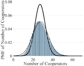
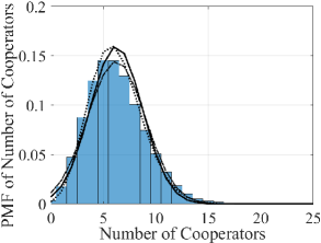
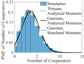
Based on [31], the skewness and kurtosis together can be employed to assess the normality of a distribution. For a Gaussian distribution, β1=β2=0subscript𝛽1subscript𝛽20\beta_{1}=\beta_{2}=0. Thus, if both β10subscript𝛽10\beta_{1}\rightarrow 0 and β20subscript𝛽20\beta_{2}\rightarrow 0, we can say that the RV could be closely approximated by a Gaussian distribution [32]. Based on (29), we see that Z𝑍Z can be approximated by a Gaussian distribution when 𝔼Φ{Z}subscript𝔼Φ𝑍{\operatorname*{\mathbb{E}}}_{\Phi}\{{Z}\}\rightarrow\infty since 𝔼Φ{Z}subscript𝔼Φ𝑍{\operatorname*{\mathbb{E}}}_{\Phi}\{{Z}\}\rightarrow\infty leads to β10subscript𝛽10\beta_{1}\rightarrow 0 and β20subscript𝛽20\beta_{2}\rightarrow 0. Using 𝔼Φ{Z}subscript𝔼Φ𝑍{\operatorname*{\mathbb{E}}}_{\Phi}\{{Z}\} and Var{Z}Var𝑍\textnormal{Var}\{Z\} derived in this subsection, we can use well-known closed-form distributions (e.g., Poisson and Gaussian distributions) to approximate the PMF and CDF of Z𝑍Z. In Sec. VI, we will use Poisson and Gaussian distributions with derived mean and variance to fit the PMF and CDF of the number of cooperators.

V-C Pairs of Two Nearest Bacteria Both Cooperating

Using the cooperating probability derived in Section IV, we evaluate the expected number of pairs of one node and its n𝑛nth nearest node to both be cooperators, which we denote by P(n)𝑃𝑛P(n). Such an expression can be used to quantify the average number of clusters of cooperators and to study the impact of a cooperative bacterium on the cooperative behaviors of its neighbors. For example, we could compare the number of pairs of two nearest bacteria both cooperating and the number of cooperators derived in Section V.B to know whether most cooperators are the only cooperators in their vicinity, which shows the impact of a cooperative bacterium on the behaviors of its neighbors. We first write P(n)𝑃𝑛P(n) as

P(n)=𝔼Φ{xiΦ(λ){Pr(B(xi,Φ)=1)Pr(B(xi,n,Φ)=1)}},𝑃𝑛subscript𝔼Φsubscriptsubscript𝑥𝑖Φ𝜆Pr𝐵subscript𝑥𝑖Φ1Pr𝐵subscript𝑥𝑖𝑛Φ1\displaystyle P(n)={\operatorname*{\mathbb{E}}}_{\Phi}\Bigg{\{}\sum_{\vec{x_{i}}\in\Phi(\lambda)}\{\textnormal{Pr}\left(B(\vec{x_{i}},\Phi)=1\right)\textnormal{Pr}\left(B(\vec{x}_{i,n},\Phi)=1\right)\}\Bigg{\}}, (30)

where xi,nsubscript𝑥𝑖𝑛\vec{x}_{i,n} is the n𝑛nth nearest node to node xisubscript𝑥𝑖\vec{x_{i}}. We derive P(n)𝑃𝑛P(n) in the following theorem.

Theorem 9

The expression of P(n)𝑃𝑛P(n) in given by

P(n)=𝑃𝑛absent\displaystyle P(n)= λ|r1|=0R1{Pr~(Nagg(r1|λ)η)|r2|=0R1ψ=02πPr~(Nagg(r2|λ)η)gn(r(r1))2πr(r1)|r2|d|r2|𝑑ψ}2π|r1|d|r1|,𝜆superscriptsubscriptsubscript𝑟10subscript𝑅1~Prsuperscriptsubscript𝑁aggconditionalsubscript𝑟1𝜆𝜂superscriptsubscriptsubscript𝑟20subscript𝑅1superscriptsubscript𝜓02𝜋~Prsuperscriptsubscript𝑁aggconditionalsubscript𝑟2𝜆𝜂subscript𝑔𝑛𝑟subscript𝑟12𝜋𝑟subscript𝑟1subscript𝑟2𝑑subscript𝑟2differential-d𝜓2𝜋subscript𝑟1𝑑subscript𝑟1\displaystyle\;\lambda\int_{|\vec{r_{1}}|=0}^{R_{1}}\bigg{\{}\widetilde{\textnormal{Pr}}\left(N_{\textnormal{agg}}^{{\dagger}}(\vec{r_{1}}|\lambda)\geq\eta\right)\int_{|\vec{r_{2}}|=0}^{R_{1}}\int_{\psi=0}^{2\pi}\widetilde{\textnormal{Pr}}\left(N_{\textnormal{agg}}^{{\dagger}}(\vec{r_{2}}|\lambda)\geq\eta\right)\frac{g_{n}(r(\vec{r_{1}}))}{2\pi r(\vec{r_{1}})}|\vec{r_{2}}|\,d|\vec{r_{2}}|\,d\psi\bigg{\}}2\pi|\vec{r_{1}}|\,d|\vec{r_{1}}|, (31)

where Pr~(Nagg(x|λ)η)~Prsuperscriptsubscript𝑁aggconditional𝑥𝜆𝜂\widetilde{\textnormal{Pr}}\left(N_{\textnormal{agg}}^{{\dagger}}(\vec{x}|\lambda)\geq\eta\right) can by obtained by replacing xisubscript𝑥𝑖\vec{x_{i}} with x𝑥\vec{x} in (IV-A) or (18).

Proof:

See Appendix K. ∎

VI Numerical Results and Simulations

In this section, we present simulation and numerical results to assess the accuracy of our derived analytical results and reveal the impact of environmental parameters on the number of molecules observed, the cooperating probability, and the statistics of the number of cooperators derived in Sections IIIV.

The simulation details are as follows. The simulation environment is unbounded. We vary density, bacteria community radius R1subscript𝑅1R_{1}, and threshold η𝜂\eta. Unless specified otherwise, we consider molecule degradation with rate k=1×101/s𝑘1superscript101sk=1\times 10^{1}/{\textnormal{s}} in the environment, a circular RX with R0=0.757μmsubscript𝑅00.757𝜇mR_{0}=0.757\,{\mu}\textnormal{m}, emission rate q=1×10³molecule/s𝑞1superscript103moleculesq=1\times 10^{3}\,{\textnormal{molecule}}/{\textnormal{s}}, and diffusion coefficient D=5.5×10¹⁰m2/s𝐷5.5superscript1010superscriptm2sD=5.5\times 10^{-10}{\textnormal{m}^{2}}/{\textnormal{s}}. The values of environment parameters are chosen to be on the same orders as those used in [21, 22, 23, 33]. In particular, the chosen value of D𝐷D is the diffusion coefficient of the 3OC6-HSL in water at room temperature [33]. The volume of a sphere with the chosen radius is approximately equal to the volume of V. fischeri444In fact, the shape of V. fischeri is a straight rod that is 0.8μm0.8𝜇m0.8\,{\mu}\textnormal{m}-1.3μm1.3𝜇m1.3\,{\mu}\textnormal{m} in diameter and 1.8μm1.8𝜇m1.8\,{\mu}\textnormal{m}-2.4μm2.4𝜇m2.4\,{\mu}\textnormal{m} in length. Due to its rod shape, we calculate its average volume as π(((0.8μm+1.3μm)/2)/2)2(1.8μm+2.4μm)/2=1.82μm3𝜋superscript0.8𝜇m1.3𝜇m2221.8𝜇m2.4𝜇m21.82𝜇superscriptm3\pi(((0.8\,{\mu}\textnormal{m}+1.3\,{\mu}\textnormal{m})/2)/2)^{2}(1.8\,{\mu}\textnormal{m}+2.4\,{\mu}\textnormal{m})/2=1.82\,{\mu}\textnormal{m}^{3}. Thus, we choose R0=0.757μmsubscript𝑅00.757𝜇mR_{0}=0.757\,{\mu}\textnormal{m} which satisfies (4/3)πR03=1.82μm343𝜋superscriptsubscript𝑅031.82𝜇superscriptm3(4/3)\pi{R_{0}}^{3}=1.82\,{\mu}\textnormal{m}^{3}.. We emphasize that these parameters are example values and the general trends of our numerical observations in the following figures do not change for other combinations of parameter values. We simulate the Brownian motion of molecules using a particle-based method as described in [34]. The molecules are initialized at the center of bacteria. The location of each molecule is updated every time step ΔtΔ𝑡\Delta t, where diffusion along each dimension is simulated by generating a normal RV with variance 2DΔt2𝐷Δ𝑡2D\Delta t. Every molecule has a chance of degrading in every time step with the probability exp(kΔt)𝑘Δ𝑡\exp(-k\Delta t). In simulations, the locations of bacteria are randomly generated according to a 2D PPP, thus the number of bacteria in different realizations is a Poisson RV and we consider that the average number of TXs or bacteria is 100 in Figs. 511. Since the time between consecutive events in a 1D PPP is exponentially distributed, we generate i.i.d. exponential RVs for each bacterium to simulate the time between consecutive molecule releases. There are also other methods to generate random release times, e.g., we could generate Poisson RVs as the numbers of release times within a fixed time duration and then uniformly distribute these release times over the fixed duration. In Fig. 4, there is one TX at a fixed location and for each realization we randomly generate molecule release times at the TX. In Figs. 511, for each realization we randomly generate both the locations and molecule release times for all TXs (bacteria).
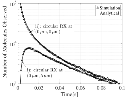
Refer to caption
(a) Impulse Emission
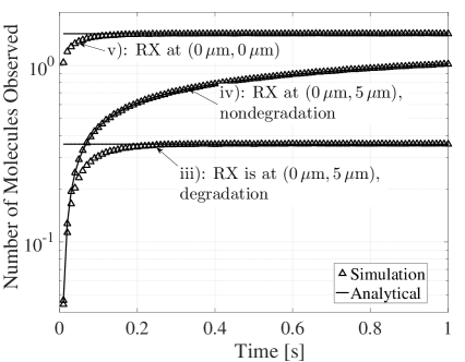
Refer to caption
(b) Continuous Emission
Figure 4: The expected number of molecules observed at the RX N¯(b,t)¯𝑁𝑏𝑡\overline{N}\left(\vec{b},t\right) versus time due to the emission of one TX located at (0,0)00(0,0). In Fig. 4(a), we consider one impulse emission with 105superscript10510^{5} molecules and molecular degradation is considered. We consider two cases of the RX in Fig. 4(a): Case i) the circular RX located at (0,5μm)05𝜇m(0,5\,{\mu}\textnormal{m}) and Case ii) the circular RX located at (0,0)00(0,0). In Fig. 4(b), we consider continuous emission and the circular RX is considered. We consider three cases of the RX in Fig. 4(b): Case iii) the RX located at (0,5μm)05𝜇m(0,5\,{\mu}\textnormal{m}) with molecular degradation, Case iv) the RX located at (5μm,0)5𝜇m0(5\,{\mu}\textnormal{m},0) without molecular degradation, and Case v) the RX located at (0,0)00(0,0) with molecular degradation.

In Fig. 4, we plot the expected number of molecules observed at the RX due to one TX’s impulse emission with 106superscript10610^{6} molecules in Fig. 4(a) and one TX’s continuous emission in Fig. 4(b). The analytical curves in Case i)–Case v) are obtained by (1), (4), (5), (7), and (6), respectively. In Fig. 4(a), we see that there is an optimal time at which channel response is maximal when the RX is not at the TX, while the channel response always decreases with time when the RX is at the TX. This is not surprising since the molecules diffuse away once released. In Fig. 4(b), we see that the channel response with molecular degradation converges as time goes to infinity, while the channel response without molecular degradation always increases with time.
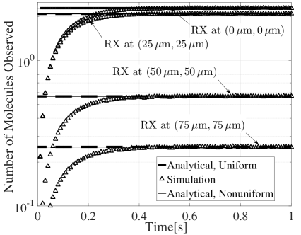
Refer to caption
(a) The Expected Number of Molecules Observed
Refer to caption
(b) The Cooperating Probability
Figure 5: The expected number of molecules observed at the RX, 𝔼Φ{N¯agg(b|λ)}subscript𝔼Φsubscript¯𝑁aggconditional𝑏𝜆{\operatorname*{\mathbb{E}}}_{\Phi}\left\{\overline{N}_{\textnormal{agg}}\left(\vec{b}|\lambda\right)\right\}, in Fig. 5(a) and the corresponding cooperating probability at the RX, Pr~(Nagg(xi|λ)η)~Prsuperscriptsubscript𝑁aggconditionalsubscript𝑥𝑖𝜆𝜂\widetilde{\textnormal{Pr}}\left(N_{\textnormal{agg}}^{{\dagger}}(\vec{x_{i}}|\lambda)\geq\eta\right), in Fig. 5(b) due to continuous emission at randomly-distributed TXs. For different environmental radii R1=50μmsubscript𝑅150𝜇mR_{1}=50\,{\mu}\textnormal{m}, R1=100μmsubscript𝑅1100𝜇mR_{1}=100\,{\mu}\textnormal{m}, and R1=150μmsubscript𝑅1150𝜇mR_{1}=150\,{\mu}\textnormal{m}, the RX’s location is (R12,R12)subscript𝑅12subscript𝑅12(\frac{R_{1}}{2},\frac{R_{1}}{2}). For R1=50μmsubscript𝑅150𝜇mR_{1}=50\,{\mu}\textnormal{m}, we also consider the RX located at the center of environment, i.e., (0,0)00(0,0).

In Fig. 5, we plot the expected number of molecules observed at the RX in Fig. 5(a) and the corresponding cooperating probability at the RX in Fig. 5(b) due to continuous emission at randomly-distributed TXs for different environmental radii. We first discuss the results in Fig. 5(a). The asymptotic curves when the RX is at (0,0)00(0,0) with the UCA and without UCA are obtained by (11) and (2), respectively. The asymptotic curves when the RX is at (R12,R12)subscript𝑅12subscript𝑅12(\frac{R_{1}}{2},\frac{R_{1}}{2}) with UCA and without UCA are obtained by (9) and (5), respectively. As observed in Fig. 4(b), we see that the expected number of molecules observed in Fig. 5(a) first increases with time and then becomes stable after some time. We then see that the asymptotic curves with UCA and without UCA almost overlap with each other. This demonstrates the accuracy of the UCA in the derivation of the asymptotic channel response where a circular field of TXs continuously emits molecules.

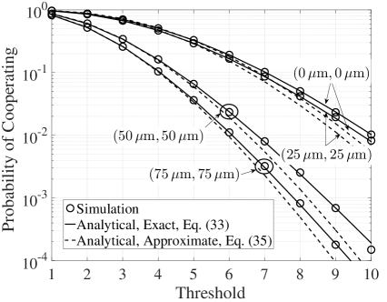
Next, we discuss the results in Fig. 5(b). The exact and approximate analytical curves are obtained by (IV-A) via (E) and (18) via (9), respectively. We see that (IV-A) is always accurate while (18) is only accurate when the probability of cooperation is relatively high, e.g., Pr~(Nagg(xi|λ)η)101~Prsuperscriptsubscript𝑁aggconditionalsubscript𝑥𝑖𝜆𝜂superscript101\widetilde{\textnormal{Pr}}\left(N_{\textnormal{agg}}^{{\dagger}}(\vec{x_{i}}|\lambda)\geq\eta\right)\geq 10^{-1}. We note that the computational complexity of (18) is much lower than that of (IV-A). Thus, in the circumstances of limited computational capabilities and high probability of cooperation, (18) is a good method to estimate the probability of cooperation. Finally, we note that when R1subscript𝑅1R_{1} decreases, the expected number of molecules and the probability of cooperation increase. This is because the density of TXs is higher when R1subscript𝑅1R_{1} is smaller.

Refer to caption
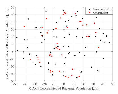
Figure 6: A realization of a 2D PPP of randomly-distributed bacteria and the resulting cooperative bacteria. R1=50μmsubscript𝑅150𝜇mR_{1}=50\,{\mu}\textnormal{m}.
Refer to caption
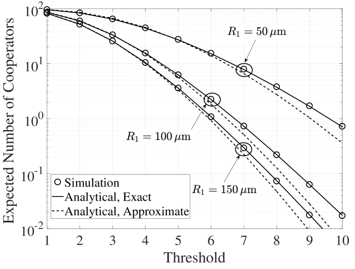
Figure 7: The expected number of cooperators over spatial PPP 𝔼Φ{Z}subscript𝔼Φ𝑍{\operatorname*{\mathbb{E}}}_{\Phi}\{Z\} versus threshold η𝜂\eta for different population radii R1subscript𝑅1R_{1}.

In Fig. 7, we simulate the decisions of bacteria under one realization of randomly-distributed bacteria locations and random molecule release times at all bacteria. We plot the spatial distribution of cooperators in this realization. In Fig. 7, we plot the first moment (i.e, the mean) of the number of cooperative bacteria versus threshold for different population radii. The exact analytical curves are obtained by (26) via (IV-A) and (E) and the approximate analytical curves are obtained by (26) via (18) and (9). We see that the curves obtained by (26) via (18) are only accurate when 𝔼Φ{Z}10subscript𝔼Φ𝑍10{\operatorname*{\mathbb{E}}}_{\Phi}\{Z\}\geq 10. This is because (18) is only accurate when Pr~(Nagg(xi|λ)η)101~Prsuperscriptsubscript𝑁aggconditionalsubscript𝑥𝑖𝜆𝜂superscript101\widetilde{\textnormal{Pr}}\left(N_{\textnormal{agg}}^{{\dagger}}(\vec{x_{i}}|\lambda)\geq\eta\right)\geq 10^{-1}, as observed in Fig. 5(b). We also see that the analytical mean obtained by (26) via (IV-A) exactly matches with simulations. This observation numerically validates Remark 3, i.e., the approximation in (I.1) is tight for the first moment of the number of cooperators. We also see that the expected number of cooperators decreases when the threshold increases, because the probability of cooperation is smaller when the threshold is higher, as observed in Fig. 5(b).
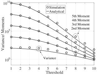
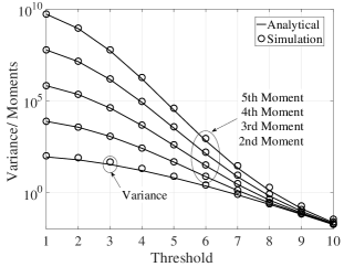
Refer to caption
(a) Moments: R1=50μmsubscript𝑅150𝜇mR_{1}=50\,{\mu}\textnormal{m}
Refer to caption
(b) Moments: R1=100μmsubscript𝑅1100𝜇mR_{1}=100\,{\mu}\textnormal{m}
Refer to caption
(c) Moments: R1=150μmsubscript𝑅1150𝜇mR_{1}=150\,{\mu}\textnormal{m}
Figure 8: The different orders of moments of number of cooperators 𝔼Φ{(Z)n}subscript𝔼Φsuperscript𝑍𝑛{\operatorname*{\mathbb{E}}}_{\Phi}\{(Z)^{n}\} versus threshold η𝜂\eta for different population radii R1subscript𝑅1R_{1}.

In Figs. 8(a)8(c), we plot the variance and moments of number of cooperators versus threshold for different population radii. The analytical variances are obtained by (27) and the analytical moments are obtained by (28) via (26). We first see that when the population density is smaller (i.e., R1subscript𝑅1R_{1} is larger), the accuracy of the analytical variances and the moments improves, thereby validating Remark 3. We then see that the curves of different moments of number of cooperators merge as the threshold increases. This can be explained by the extreme case that the different moments of the number of cooperators would tend to zero as the threshold continually increases, leading to the fact that different moments of the number of cooperators become the same as the threshold continually increases.
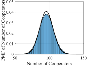
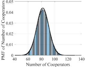
Refer to caption
(a) R1=50μmsubscript𝑅150𝜇mR_{1}=50\,{\mu}\textnormal{m}, η=1𝜂1\eta=1
Refer to caption
(b) R1=100μmsubscript𝑅1100𝜇mR_{1}=100\,{\mu}\textnormal{m}, η=1𝜂1\eta=1
Refer to caption
(c) R1=150μmsubscript𝑅1150𝜇mR_{1}=150\,{\mu}\textnormal{m}, η=1𝜂1\eta=1
Refer to caption
(d) R1=50μmsubscript𝑅150𝜇mR_{1}=50\,{\mu}\textnormal{m}, η=5𝜂5\eta=5
Refer to caption
(e) R1=100μmsubscript𝑅1100𝜇mR_{1}=100\,{\mu}\textnormal{m}, η=5𝜂5\eta=5
Refer to caption
(f) R1=150μmsubscript𝑅1150𝜇mR_{1}=150\,{\mu}\textnormal{m}, η=5𝜂5\eta=5
Figure 9: The PMF of number of cooperators for different population radii R1subscript𝑅1R_{1} and different thresholds η𝜂\eta.
TABLE I: Deviation between Simulation and Analytical Values at Peak PMF in Fig. 9.
(a) (b) (c) (d) (e) (f)
Poisson Approximation 6.01%percent6.016.01\% 5.09%percent5.095.09\% 6.02%percent6.026.02\% 45.42%percent45.4245.42\% 9.65%percent9.659.65\% 1.77%percent1.771.77\%
Gaussian Approximation 6.01%percent6.016.01\% 5.09%percent5.095.09\% 6.04%percent6.046.04\% 48.23%percent48.2348.23\% 10.20%percent10.2010.20\% 4.01%percent4.014.01\%

We investigate the distributions of the simulated number of cooperators using the statistical distribution fitting software EasyFit555 http://www.mathwave.com/easyfit-distribution-fitting.html. We find that the simulated number of cooperators can be generally well fitted by Beta, Johnson SB, Normal (Gaussian), and Gamma distributions when the number of cooperators is large. When the number of cooperators is small, the simulated number of cooperators can be generally well fitted by Poisson and Binomial distributions. We note that Gaussian and Poisson distributions are the most convenient distributions among them while achieving good fitting accuracy. Hence, we use the Gaussian and Poisson distributions with our derived mean and variance to analytically fit the simulated distribution of cooperators in Fig. 9 for assessing its accuracy to analytically predict the distribution of cooperators.

In Fig. 9, we use the Poisson and Gaussian distributions with analytical mean 𝔼Φ{Z}subscript𝔼Φ𝑍{\operatorname*{\mathbb{E}}}_{\Phi}\{Z\} and variance Var{Z}Var𝑍\textnormal{Var}\{Z\} shown in Fig. 8 to fit the PMF of simulated number of cooperators. To quantitatively assess the accuracy of Poisson and Gaussian approximations, we calculate the deviation between the simulation and analytical curves by |analysissimulation|/simulationanalysissimulationsimulation{|\textrm{analysis}-\textrm{simulation}|}/{\textrm{simulation}}. We are interested in the deviation at the peak PMF since such deviation is the largest difference across the whole range of the PMF. The calculated deviation for different cases in Fig. 9 is listed in Table I. Based on Table I, we see that the distribution of the number of cooperators can generally be well approximated by the Poisson and Gaussian distributions, especially when the expected number is relatively large, which meets our expectations discussed in Sec. V-B. When the number of cooperators is relatively small, e.g., Z<15𝑍15Z<15, the Poisson approximation has better accuracy than the Gaussian approximation. This observation is also expected since the continuous Gaussian distribution is an approximation of the discrete distribution and such approximation is more accurate when the number of cooperators is higher. The deviation between the Poisson and Gaussian distributions and simulated distribution for R1=50μmsubscript𝑅150𝜇mR_{1}=50\,{\mu}\textnormal{m} and η=5𝜂5\eta=5 is caused by the deviation between the analytical variance and simulated variance, as observed in Fig. 8(a).
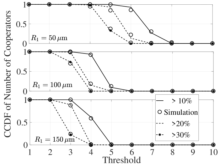
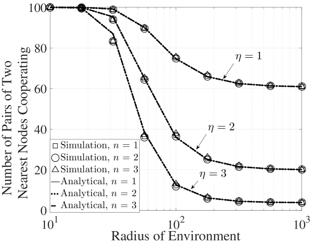
Refer to caption
Figure 10: The CCDF that the number of cooperators versus threshold η𝜂\eta for different population radii R1subscript𝑅1R_{1}.
Refer to caption
Figure 11: The number of pairs of any node and its n𝑛nth nearest node both cooperating versus the population radius.

In Fig. 11, we plot the complementary CDF (CCDF) of the number of cooperators versus threshold for different population radii. These CCDFs could be interpreted as the probability of success to activate a colony of bacteria if we can define the activation of the colony as a minimal number of cells (i.e., fraction of the colony) being activated. The probability of success indicates the overall activation level of a colony, e.g., the likelihood of the colony forming a biofilm. The analytical curves are obtained by the CCDF of the Poisson distribution with analytical mean 𝔼Φ{Z}subscript𝔼Φ𝑍{\operatorname*{\mathbb{E}}}_{\Phi}\{Z\} and variance Var{Z}Var𝑍\textnormal{Var}\{Z\} shown in Fig. 8, respectively. We see that the CCDF of the number of cooperators can be well approximated by that of the Poisson distributions. We also see that the CCDF of the number of cooperators decreases as the threshold increases. The PMF and CDF in Figs. 9 and 11 indicates that the Poisson and Gaussian approximations can be used to not only accurately model the distribution of the number of observed molecules as many MC works have done, e.g., [35, 25, 36], but also model the distribution of the number of cooperative bacteria in QS with good accuracy. Therefore, the easy-to-use Poisson and Gaussian distributions with our derived mean and variance serve as powerful tools to predict the group behavior of bacteria in QS and control their group behavior by adjusting the environmental parameters, e.g., diffusion coefficient and chemical reaction rate. Thus, our research plays as an important role in advancing numerous QS-related healthcare and environmental applications, e.g., preventing the formation of biofilms in antibiotic resistance and understanding the bioluminescene in environmental monitoring.

In Fig. 11, we plot the number of pairs of any node and its n𝑛nth nearest node both cooperating P(n)𝑃𝑛P(n) versus the population radius R1subscript𝑅1R_{1} for different thresholds η𝜂\eta. The analytical curves are obtained by (31). We first see that for the same threshold η𝜂\eta, the curves of P(n)𝑃𝑛P(n) with different n𝑛n almost overlap. This is because bacteria are randomly distributed and the observations among different bacteria are independent. This observation is not intuitive, which suggests that the distance between bacteria has a minor impact on the average number of clusters of cooperators. Second, we see that the curves of P(n)𝑃𝑛P(n) first decrease and then converge to a constant number as the population radius R1subscript𝑅1R_{1} increases. This is because when the population radius increases, the number of molecules observed by the bacteria decreases, but as the population radius tends to infinity, the molecules received by any bacterium is dominated by the molecules released from itself and the number of molecules received by any bacterium converges to a constant number. This observation suggests that the density of bacteria has a marginal impact on the average number of clusters of cooperators when the density is very low.

VII Conclusions

In this work, we provided an analytically-tractable model for predicting the concentration of molecules observed by bacteria and the statistics of the number of responsive cooperative bacteria, by taking the motion of molecules undergoing independent diffusion and degradation into consideration. We adopted some assumptions to capture the basic features of QS, e.g., random bacterial location, random molecular emission times, and each bacterium both acting as a TX and a RX. Upon these realistic assumptions, the 2D channel response and the expected probability of cooperation at a bacterium due to continuous emission of molecules at randomly-distributed bacteria were derived. The different order moments and cumulants, the CDF and PMF of the number of cooperators, and the number of pairs of two bacteria both cooperating, were also derived. Since we considered molecular propagation channels among a population of bacteria, the impact of environmental factors on the QS process could be predicted, e.g., environment temperature and pH can affect the diffusion coefficient and degradation rate, respectively.

Interesting future works include relaxing these simplifications, and validating our theoretical model using lab experiments in a 2D environment. Potential experimental setups for validation may include bacteria strains in plastic Petri dishes, bioluminescence monitoring systems that detect cooperative bacteria concentrations by their light emission [37], and computers for post-processing and analysis. Modeling multiple species of bacteria in QS is also interesting future work since multispecies QS signals may inhibit quorum sensing activation [2]. For example, some types of bacteria produce enzymes that destroy quorum sensing signals of other types of bacteria. Such inhibition could lead to lower cooperative probabilities and fewer cooperators compared to the case when QS is in the absence of the bacteria that release the destructive enzymes. Finally, we note that our analytically-tractable model could be readily extended to a three-dimensional (3D) environment by changing the 2D area integrations to 3D volume integrations.

Appendix A Proof of Proposition 1

To prove (2), we have

N¯(b,t)=(a)𝔼{τ[0,t]N¯im(b,tτ)}=(b)qτ=0tN¯im(b,tτ)𝑑τ=(c)qτ=0tN¯im(b,τ)𝑑τ,¯𝑁𝑏𝑡𝑎𝔼subscript𝜏0𝑡subscript¯𝑁im𝑏𝑡𝜏𝑏𝑞superscriptsubscript𝜏0𝑡subscript¯𝑁im𝑏𝑡𝜏differential-d𝜏𝑐𝑞superscriptsubscript𝜏0𝑡subscript¯𝑁im𝑏𝜏differential-d𝜏\displaystyle\overline{N}\left(\vec{b},t\right)\overset{(a)}{=}\operatorname*{\mathbb{E}}\Bigg{\{}\sum_{\tau\in[0,t]}\overline{N}_{\textnormal{im}}\left(\vec{b},t-\tau\right)\Bigg{\}}\overset{(b)}{=}q\int_{\tau=0}^{t}\overline{N}_{\textnormal{im}}\left(\vec{b},t-\tau\right)d\tau\overset{(c)}{=}q\int_{\tau=0}^{t}\overline{N}_{\textnormal{im}}\left(\vec{b},\tau\right)d\tau, (A.1)

where N¯im(b,tτ)subscript¯𝑁im𝑏𝑡𝜏\overline{N}_{\textnormal{im}}\left(\vec{b},t-\tau\right) is the channel response observed at time t𝑡t due to the one molecule emitted at time τ𝜏\tau and τ𝜏\tau is a random time instant on a real line [0,t]0𝑡[0,t] distributed according to a 1D PPP with density (rate) q𝑞q. Equality (a) exploits the fact that the channel response at time t𝑡t due to continuous emission is equal to the expected sum of all channel responses due to all impulse emissions at different random time instants. Equality (b) is obtained by applying Campbell’s Theorem and equality (c) is obtained by applying a variable transformation. By taking the limit t𝑡t\rightarrow\infty in (A.1), we obtain (2).

Appendix B Proof of Theorem 1 and Theorem 2

To prove (1), we have

N¯im(b,τ)=(a)subscript¯𝑁im𝑏𝜏𝑎\displaystyle\overline{N}_{\textnormal{im}}\left(\vec{b},\tau\right)\overset{(a)}{=} r=0R0θ=02πC(r1,τ)r𝑑θ𝑑r=r=0R0θ=02π1(4πDτ)exp(|r1|24Dτkτ)r𝑑θ𝑑rsuperscriptsubscript𝑟0subscript𝑅0superscriptsubscript𝜃02𝜋𝐶subscript𝑟1𝜏𝑟differential-d𝜃differential-d𝑟superscriptsubscript𝑟0subscript𝑅0superscriptsubscript𝜃02𝜋14𝜋𝐷𝜏superscriptsubscript𝑟124𝐷𝜏𝑘𝜏𝑟differential-d𝜃differential-d𝑟\displaystyle\;\int_{r=0}^{R_{0}}\int_{\theta=0}^{2\pi}C\left(\vec{r_{1}},\tau\right)rd\theta dr=\int_{r=0}^{R_{0}}\int_{\theta=0}^{2\pi}\frac{1}{(4\pi D\tau)}\exp\left(-\frac{|\vec{r_{1}}|^{2}}{4D\tau}-k\tau\right)rd\theta dr
=\displaystyle= r=0R0θ=02π1(4πDτ)exp(|b|2+r2+2|b|rcosθ4Dτkτ)r𝑑θ𝑑rsuperscriptsubscript𝑟0subscript𝑅0superscriptsubscript𝜃02𝜋14𝜋𝐷𝜏superscript𝑏2superscript𝑟22𝑏𝑟𝜃4𝐷𝜏𝑘𝜏𝑟differential-d𝜃differential-d𝑟\displaystyle\;\int_{r=0}^{R_{0}}\int_{\theta=0}^{2\pi}\frac{1}{(4\pi D\tau)}\exp\left(-\frac{{|\vec{b}|}^{2}+r^{2}+2{|\vec{b}|}r\cos\theta}{4D\tau}-k\tau\right)rd\theta dr
=(b)𝑏\displaystyle\overset{(b)}{=} 14πDexp(kτ)r=0R0rτexp(|b|2+r24Dτ)2πI0(|b|r2Dτ)𝑑r14𝜋𝐷𝑘𝜏superscriptsubscript𝑟0subscript𝑅0𝑟𝜏superscript𝑏2superscript𝑟24𝐷𝜏2𝜋subscript𝐼0𝑏𝑟2𝐷𝜏differential-d𝑟\displaystyle\;\frac{1}{4\pi D}\exp(-k\tau)\int_{r=0}^{R_{0}}\frac{r}{\tau}\exp\left(-\frac{{|\vec{b}|}^{2}+r^{2}}{4D\tau}\right)2\pi I_{0}\left(\frac{|\vec{b}|r}{2D\tau}\right)dr
(c)𝑐\displaystyle\overset{(c)}{\approx} i=14{12Dexp(kτ)r=0R0rτexp(|b|2+r24Dτ)αiexp(βi|b|r2Dτ)𝑑r}superscriptsubscript𝑖1412𝐷𝑘𝜏superscriptsubscript𝑟0subscript𝑅0𝑟𝜏superscript𝑏2superscript𝑟24𝐷𝜏subscript𝛼𝑖subscript𝛽𝑖𝑏𝑟2𝐷𝜏differential-d𝑟\displaystyle\;\sum_{i=1}^{4}\bigg{\{}\frac{1}{2D}\exp(-k\tau)\int_{r=0}^{R_{0}}\frac{r}{\tau}\exp\bigg{(}-\frac{{|\vec{b}|}^{2}+r^{2}}{4D\tau}\bigg{)}\alpha_{i}\exp\left(\beta_{i}\frac{|\vec{b}|r}{2D\tau}\right)dr\bigg{\}} (B.1)

where C(r,τ)=1(4πDτ)exp(|r|24Dτkτ)𝐶𝑟𝜏14𝜋𝐷𝜏superscript𝑟24𝐷𝜏𝑘𝜏C\left(\vec{r},\tau\right)=\frac{1}{\left(4\pi D\tau\right)}\exp\left(-\frac{|\vec{r}|^{2}}{4D\tau}-k\tau\right) [38, eq. (3.4)] is the channel response at the point defined by r𝑟\vec{r} at the time τ𝜏\tau due to an impulse emission of one molecule from the point at (0,0)00(0,0) at time τ=0𝜏0\tau=0 into an unbounded 2D environment. Equality (a) is due to the fact that N¯im(b,τ)subscript¯𝑁im𝑏𝜏\overline{N}_{\textnormal{im}}\left(\vec{b},\tau\right) for a circular passive observer S0subscript𝑆0S_{0} centered at b𝑏\vec{b} can be obtained by integrating C(r1,τ)𝐶subscript𝑟1𝜏C\left(\vec{r_{1}},\tau\right) over S0subscript𝑆0S_{0}, where r1subscript𝑟1\vec{r_{1}} is a vector from (0,0)00(0,0) to a point within the RX S0subscript𝑆0S_{0}. Equality (b) is obtained by applying [17, eq. (3.339)] and equality (c) is obtained by applying I0(z)i=14αiexp(βiz)subscript𝐼0𝑧superscriptsubscript𝑖14subscript𝛼𝑖subscript𝛽𝑖𝑧I_{0}(z)\approx\sum_{i=1}^{4}\alpha_{i}\exp(\beta_{i}z) [27, eq. (7)]. Calculating the final expression of (B), we obtain (1). To prove (4), we simplify (B) using |b|=0𝑏0|\vec{b}|=0 as

N¯im,self(τ)=r=0R0θ=02πexp(r24Dτkτ)(4πDτ)𝑑θ𝑑r=r=0R0r(2Dτ)exp(r24Dτkτ)𝑑r.subscript¯𝑁imself𝜏superscriptsubscript𝑟0subscript𝑅0superscriptsubscript𝜃02𝜋superscript𝑟24𝐷𝜏𝑘𝜏4𝜋𝐷𝜏differential-d𝜃differential-d𝑟superscriptsubscript𝑟0subscript𝑅0𝑟2𝐷𝜏superscript𝑟24𝐷𝜏𝑘𝜏differential-d𝑟\displaystyle\overline{N}_{\textnormal{im},\textnormal{self}}\left(\tau\right)=\int_{r=0}^{R_{0}}\int_{\theta=0}^{2\pi}\frac{\exp\left(-\frac{r^{2}}{4D\tau}-k\tau\right)}{(4\pi D\tau)}\,d\theta\,dr=\int_{r=0}^{R_{0}}\frac{r}{(2D\tau)}\exp\left(-\frac{r^{2}}{4D\tau}-k\tau\right)\,dr. (B.2)

We then apply [17, eq. (2.33.12)] to (B.2) to solve it as (4), which completes the proof.

Appendix C Proof of Theorem 3 and Theorem 4

We first prove (5). Based on (2), the channel response due to continuous emission in (5) can be obtained by integrating the impulse channel response over time, but integrating (1) over τ𝜏\tau incurs very high complexity. Thus, we simplify (1) by considering UCA within the circular RX. i.e., N¯im(b,τ)πR02C(b,τ)subscript¯𝑁im𝑏𝜏𝜋superscriptsubscript𝑅02𝐶𝑏𝜏\overline{N}_{\textnormal{im}}\left(\vec{b},\tau\right)\approx\pi R_{0}^{2}C\left(\vec{b},\tau\right). Based on (2) and the UCA, we evaluate N¯(b,)¯𝑁𝑏\overline{N}\left(\vec{b},\infty\right) as

N¯(b,)πR02τ=0qC(b,τ)𝑑τπR02qτ=01(4πDτ)exp(|b|24Dτkτ)𝑑τ.¯𝑁𝑏𝜋superscriptsubscript𝑅02superscriptsubscript𝜏0𝑞𝐶𝑏𝜏differential-d𝜏𝜋superscriptsubscript𝑅02𝑞superscriptsubscript𝜏014𝜋𝐷𝜏superscript𝑏24𝐷𝜏𝑘𝜏differential-d𝜏\displaystyle\overline{N}\left(\vec{b},\infty\right)\approx\pi R_{0}^{2}\int_{\tau=0}^{\infty}qC\left(\vec{b},\tau\right)d\tau\approx\pi R_{0}^{2}q\int_{\tau=0}^{\infty}\frac{1}{\left(4\pi D\tau\right)}\exp\left(-\frac{|\vec{b}|^{2}}{4D\tau}-k\tau\right)d\tau. (C.1)

We then employ 0xν1exp(βxγx)𝑑x=2(βγ)ν2Kν(2βγ)superscriptsubscript0superscript𝑥𝜈1𝛽𝑥𝛾𝑥differential-d𝑥2superscript𝛽𝛾𝜈2subscript𝐾𝜈2𝛽𝛾\int_{0}^{\infty}x^{\nu-1}\exp\left(-\frac{\beta}{x}-\gamma x\right)dx=2\left(\frac{\beta}{\gamma}\right)^{\frac{\nu}{2}}K_{\nu}(2\sqrt{\beta\gamma}) [17, eq. (3.471)] to solve (C.1) as (5). To prove (6), we apply (4), =0exp(px)𝑑x=1/psuperscriptsubscriptabsent0𝑝𝑥differential-d𝑥1𝑝\int_{=0}^{\infty}\exp(-px)dx={1}/{p} [17, eq. (3.310)], and 0exp(βxγx)𝑑x=βγK1(βγ)superscriptsubscript0𝛽𝑥𝛾𝑥differential-d𝑥𝛽𝛾subscript𝐾1𝛽𝛾\int_{0}^{\infty}\exp\left(-\frac{\beta}{x}-\gamma x\right)dx=\frac{\beta}{\gamma}K_{1}(\sqrt{\beta\gamma}) [17, eq. (3.324.1)] to (2), we evaluate N¯self()subscript¯𝑁self\overline{N}_{\textnormal{self}}\left(\infty\right) as (6). This completes the proof.

Appendix D Proof of Theorem 5

Using Campbell’s theorem [39], we first write

𝔼Φ{N¯agg(b|λ)}=𝔼Φ{aΦ(λ)N¯(b|a)}=|r|=0R1φ=02πN¯(b|r)λ|r|𝑑φd|r|,subscript𝔼Φsubscript¯𝑁aggconditional𝑏𝜆subscript𝔼Φsubscript𝑎Φ𝜆¯𝑁conditional𝑏𝑎superscriptsubscript𝑟0subscript𝑅1superscriptsubscript𝜑02𝜋¯𝑁conditional𝑏𝑟𝜆𝑟differential-d𝜑𝑑𝑟\displaystyle{\operatorname*{\mathbb{E}}}_{\Phi}\bigg{\{}\overline{N}_{\textnormal{agg}}\left(\vec{b}|\lambda\right)\bigg{\}}={\operatorname*{\mathbb{E}}}_{\Phi}\Bigg{\{}\sum_{\vec{a}\in\Phi(\lambda)}\overline{N}\Big{(}\vec{b}|\vec{a}\Big{)}\Bigg{\}}=\int_{|\vec{r}|=0}^{R_{1}}\int_{\varphi=0}^{2\pi}\overline{N}\Big{(}\vec{b}|\vec{r}\Big{)}\lambda|\vec{r}|\,d\varphi\,d|\vec{r}|, (D.1)

where r𝑟\vec{r} is a vector from (0,0)00(0,0) to a point within the population circle S1subscript𝑆1S_{1} and φ𝜑\varphi is the supplement of the angle between r𝑟\vec{r} and b𝑏\vec{b}. We note that N¯(b|r)¯𝑁conditional𝑏𝑟\overline{N}\left(\vec{b}|\vec{r}\right) is obtained by multiplying the point channel response by the emission rate q𝑞q, integrating over S0subscript𝑆0S_{0}, and then integrating over all time, i.e.,

N¯(b|r)=¯𝑁conditional𝑏𝑟absent\displaystyle\overline{N}\left(\vec{b}|\vec{r}\right)= τ=0|r0|=0R0θ=02πqC(d,τ)|r0|𝑑θd|r0|𝑑τ,superscriptsubscript𝜏0superscriptsubscriptsubscript𝑟00subscript𝑅0superscriptsubscript𝜃02𝜋𝑞𝐶𝑑𝜏subscript𝑟0differential-d𝜃𝑑subscript𝑟0differential-d𝜏\displaystyle\int_{\tau=0}^{\infty}\int_{|\vec{r_{0}}|=0}^{R_{0}}\int_{\theta=0}^{2\pi}qC\left(\vec{d},\tau\right)|\vec{r_{0}}|\,d\theta\,d|\vec{r_{0}}|\,d\tau,
=\displaystyle= τ=0|r0|=0R0θ=02πq(4πDτ)exp(|d|24Dτkτ)|r0|𝑑θd|r0|𝑑τ,superscriptsubscript𝜏0superscriptsubscriptsubscript𝑟00subscript𝑅0superscriptsubscript𝜃02𝜋𝑞4𝜋𝐷𝜏superscript𝑑24𝐷𝜏𝑘𝜏subscript𝑟0differential-d𝜃𝑑subscript𝑟0differential-d𝜏\displaystyle\int_{\tau=0}^{\infty}\int_{|\vec{r_{0}}|=0}^{R_{0}}\int_{\theta=0}^{2\pi}\frac{q}{(4\pi D\tau)}\exp\left(-\frac{|\vec{d}|^{2}}{4D\tau}-k\tau\right)|\vec{r_{0}}|\,d\theta\,d|\vec{r_{0}}|\,d\tau,
=\displaystyle= τ=0|r0|=0R0θ=02πq(4πDτ)exp(|l|2+|r0|2+2|l||r0|cosθ4Dτkτ)|r0|𝑑θd|r0|𝑑τ,superscriptsubscript𝜏0superscriptsubscriptsubscript𝑟00subscript𝑅0superscriptsubscript𝜃02𝜋𝑞4𝜋𝐷𝜏superscript𝑙2superscriptsubscript𝑟022𝑙subscript𝑟0𝜃4𝐷𝜏𝑘𝜏subscript𝑟0differential-d𝜃𝑑subscript𝑟0differential-d𝜏\displaystyle\int_{\tau=0}^{\infty}\!\int_{|\vec{r_{0}}|=0}^{R_{0}}\!\int_{\theta=0}^{2\pi}\!\frac{q}{(4\pi D\tau)}\exp\left(\!-\frac{|\vec{l}|^{2}+|\vec{r_{0}}|^{2}+2|\vec{l}||\vec{r_{0}}|\cos\theta}{4D\tau}-k\tau\!\right)|\vec{r_{0}}|\,d\theta\,d|\vec{r_{0}}|\,d\tau, (D.2)

where l𝑙\vec{l} is a vector from r𝑟\vec{r} to b𝑏\vec{b}, i.e., l=br𝑙𝑏𝑟\vec{l}=\vec{b}-\vec{r}, r0subscript𝑟0\vec{r_{0}} is a vector from b𝑏\vec{b} to a point within the RX circle S0subscript𝑆0S_{0}, d𝑑\vec{d} is a vector from r𝑟\vec{r} to r0subscript𝑟0\vec{r_{0}}, and θ𝜃\theta is the supplement of the angle between l𝑙\vec{l} and r0subscript𝑟0\vec{r_{0}}. According to the law of cosines, we obtain |l|2=|b|2+|r|2+2|b||r|cosφsuperscript𝑙2superscript𝑏2superscript𝑟22𝑏𝑟𝜑|\vec{l}|^{2}={|\vec{b}|}^{2}+|\vec{r}|^{2}+2{|\vec{b}|}|\vec{r}|\cos\varphi and |d|2=|l|2+|r0|2+2|l||r0|cosθsuperscript𝑑2superscript𝑙2superscriptsubscript𝑟022𝑙subscript𝑟0𝜃|\vec{d}|^{2}=|\vec{l}|^{2}+|\vec{r_{0}}|^{2}+2|\vec{l}||\vec{r_{0}}|\cos\theta. We then apply |l|=|b|2+|r|2+2|b||r|cosφ𝑙superscript𝑏2superscript𝑟22𝑏𝑟𝜑|\vec{l}|=\sqrt{{|\vec{b}|}^{2}+|\vec{r}|^{2}+2{|\vec{b}|}|\vec{r}|\cos\varphi} to rewrite (D) as

N¯(b|r)=¯𝑁conditional𝑏𝑟absent\displaystyle\overline{N}\left(\vec{b}|\vec{r}\right)= τ=0|r0|=0R0θ=02πq(4πDτ)exp(Υ2(b)4Dτkτ)|r0|𝑑θd|r0|𝑑τsuperscriptsubscript𝜏0superscriptsubscriptsubscript𝑟00subscript𝑅0superscriptsubscript𝜃02𝜋𝑞4𝜋𝐷𝜏superscriptΥ2𝑏4𝐷𝜏𝑘𝜏subscript𝑟0differential-d𝜃𝑑subscript𝑟0differential-d𝜏\displaystyle\;\int_{\tau=0}^{\infty}\int_{|\vec{r_{0}}|=0}^{R_{0}}\int_{\theta=0}^{2\pi}\frac{q}{(4\pi D\tau)}\exp\left(-\frac{\Upsilon^{2}(\vec{b})}{4D\tau}-k\tau\right)|\vec{r_{0}}|\,d\theta\,d|\vec{r_{0}}|\,d\tau
=(a)𝑎\displaystyle\overset{(a)}{=} |r0|=0R0θ=02πq2DπK0(kDΥ(b))|r0|𝑑θd|r0|,superscriptsubscriptsubscript𝑟00subscript𝑅0superscriptsubscript𝜃02𝜋𝑞2𝐷𝜋subscript𝐾0𝑘𝐷Υ𝑏subscript𝑟0differential-d𝜃𝑑subscript𝑟0\displaystyle\;\int_{|\vec{r_{0}}|=0}^{R_{0}}\int_{\theta=0}^{2\pi}\frac{q}{2D\pi}K_{0}\left(\sqrt{\frac{k}{D}}\Upsilon(\vec{b})\right)|\vec{r_{0}}|\,d\theta\,d|\vec{r_{0}}|, (D.3)

where equality (c) is obtained by applying [17, eq. (3.471)]. We finally substitute (D) into (D.1) and arrive at (5). This completes the proof.

Appendix E Proof of Corollary 1, Corollary 2, and Corollary 3

We first prove (9). Using UCA, we have

N¯(b|r)¯𝑁conditional𝑏𝑟absent\displaystyle\overline{N}\left(\vec{b}|\vec{r}\right)\approx (τ=0qC(l,τ)𝑑τ)πR02τ=0qπR02(4πDτ)exp(|b|2+|r|2+2|b||r|cosφ4Dτkτ)𝑑τ,superscriptsubscript𝜏0𝑞𝐶𝑙𝜏differential-d𝜏𝜋superscriptsubscript𝑅02superscriptsubscript𝜏0𝑞𝜋superscriptsubscript𝑅024𝜋𝐷𝜏superscript𝑏2superscript𝑟22𝑏𝑟𝜑4𝐷𝜏𝑘𝜏differential-d𝜏\displaystyle\;\left(\int_{\tau=0}^{\infty}qC\left(\vec{l},\tau\right)\,d\tau\right)\pi{R_{0}}^{2}\approx\int_{\tau=0}^{\infty}\frac{q\pi{R_{0}}^{2}}{(4\pi D\tau)}\exp\left(-\frac{{|\vec{b}|}^{2}+|\vec{r}|^{2}+2{|\vec{b}|}|\vec{r}|\cos\varphi}{4D\tau}-k\tau\right)d\tau,
\displaystyle\approx qR022DK0(kDΩ(b)).𝑞superscriptsubscript𝑅022𝐷subscript𝐾0𝑘𝐷Ω𝑏\displaystyle\;\frac{q{R_{0}}^{2}}{2D}K_{0}\left(\sqrt{\frac{k}{D}\Omega(\vec{b})}\right). (E.1)

We then substitute (E) into (D.1) and obtain (9). (2) can be proven by applying |b|=0𝑏0|\vec{b}|=0 to (5). To prove (11), we apply |b|=0𝑏0|\vec{b}|=0 to (9) to rewrite (9) as (E.2). By evaluating the final expression of (E.2), we obtain (11).

𝔼Φ{N¯agg(b|λ)}||b|=0|r|=0R1φ=02πqR022DK0(kD|r|)λ|r|𝑑φd|r||r|=0R1qπR02DK0(kD|r|)λ|r|d|r|.evaluated-atsubscript𝔼Φsubscript¯𝑁aggconditional𝑏𝜆𝑏0superscriptsubscript𝑟0subscript𝑅1superscriptsubscript𝜑02𝜋𝑞superscriptsubscript𝑅022𝐷subscript𝐾0𝑘𝐷𝑟𝜆𝑟differential-d𝜑𝑑𝑟superscriptsubscript𝑟0subscript𝑅1𝑞𝜋superscriptsubscript𝑅02𝐷subscript𝐾0𝑘𝐷𝑟𝜆𝑟𝑑𝑟\displaystyle{\operatorname*{\mathbb{E}}}_{\Phi}\{\overline{N}_{\textnormal{agg}}(\vec{b}|\lambda)\}\Big{|}_{|\vec{b}|=0}\!\!\approx\!\!\int_{|\vec{r}|=0}^{R_{1}}\!\int_{\varphi=0}^{2\pi}\!\frac{q{R_{0}}^{2}}{2D}K_{0}\!\left(\!\!\sqrt{\frac{k}{D}}|\vec{r}|\!\right)\!\lambda|\vec{r}|\,d\varphi\,d|\vec{r}|\!\approx\!\int_{|\vec{r}|=0}^{R_{1}}\!\!\frac{q\pi{R_{0}}^{2}}{D}K_{0}\!\left(\!\!\sqrt{\frac{k}{D}}|\vec{r}|\!\right)\!\lambda|\vec{r}|\,d|\vec{r}|. (E.2)

Appendix F Proof of Lemma 1

We rewrite (12) as

Pr~(Nagg(xi|λ)η)=(a)1𝔼Φ{n=0η11n!exp{N¯agg(xi|λ)}(N¯agg(xi|λ))n}~Prsuperscriptsubscript𝑁aggconditionalsubscript𝑥𝑖𝜆𝜂𝑎1subscript𝔼Φsuperscriptsubscript𝑛0𝜂11𝑛superscriptsubscript¯𝑁aggconditionalsubscript𝑥𝑖𝜆superscriptsuperscriptsubscript¯𝑁aggconditionalsubscript𝑥𝑖𝜆𝑛\displaystyle\;\widetilde{\textnormal{Pr}}\left(N_{\textnormal{agg}}^{{\dagger}}(\vec{x_{i}}|\lambda)\geq\eta\right)\overset{(a)}{=}1-{\operatorname*{\mathbb{E}}}_{\Phi}\Bigg{\{}\sum_{n=0}^{\eta-1}\frac{1}{n!}\exp\left\{-\overline{N}_{\textnormal{agg}}^{{\dagger}}(\vec{x_{i}}|\lambda)\right\}\left(\overline{N}_{\textnormal{agg}}^{{\dagger}}(\vec{x_{i}}|\lambda)\right)^{n}\Bigg{\}}
=(b)𝑏\displaystyle\!\overset{(b)}{=}\!  1n=0η11n!𝔼Φ{nexp{N¯agg(xi|λ)ρ}ρn|ρ=1}=(c)1n=0η11n!n𝔼Φ{exp{N¯agg(xi|λ)ρ}}ρn|ρ=1,1superscriptsubscript𝑛0𝜂11𝑛subscript𝔼Φevaluated-atsuperscript𝑛superscriptsubscript¯𝑁aggconditionalsubscript𝑥𝑖𝜆𝜌superscript𝜌𝑛𝜌1𝑐1evaluated-atsuperscriptsubscript𝑛0𝜂11𝑛superscript𝑛subscript𝔼Φsuperscriptsubscript¯𝑁aggconditionalsubscript𝑥𝑖𝜆𝜌superscript𝜌𝑛𝜌1\displaystyle\;1-\sum_{n=0}^{\eta-1}\frac{1}{n!}{\operatorname*{\mathbb{E}}}_{\Phi}\Bigg{\{}\frac{\partial^{n}\exp\left\{\overline{N}_{\textnormal{agg}}^{{\dagger}}(\vec{x_{i}}|\lambda)\rho\right\}}{\partial\rho^{n}}\Bigg{|}_{\rho=-1}\Bigg{\}}\!\overset{(c)}{=}\!1-\sum_{n=0}^{\eta-1}\frac{1}{n!}\frac{\partial^{n}{\operatorname*{\mathbb{E}}}_{\Phi}\Big{\{}\exp\left\{\overline{N}_{\textnormal{agg}}^{{\dagger}}(\vec{x_{i}}|\lambda)\rho\right\}\Big{\}}}{\partial\rho^{n}}\Bigg{|}_{\rho=-1}, (F.1)

where equality (a) is due to the CDF of Poisson RV Nagg(xi|λ)superscriptsubscript𝑁aggconditionalsubscript𝑥𝑖𝜆N_{\textnormal{agg}}^{{\dagger}}(\vec{x_{i}}|\lambda). Equality (b) is due to exchanging the order of sum and expectation and exp{N¯agg(xi|λ)}(N¯agg(xi|λ))n=nexp{N¯agg(xi|λ)ρ}ρn|ρ=1superscriptsubscript¯𝑁aggconditionalsubscript𝑥𝑖𝜆superscriptsuperscriptsubscript¯𝑁aggconditionalsubscript𝑥𝑖𝜆𝑛evaluated-atsuperscript𝑛superscriptsubscript¯𝑁aggconditionalsubscript𝑥𝑖𝜆𝜌superscript𝜌𝑛𝜌1\exp\left\{-\overline{N}_{\textnormal{agg}}^{{\dagger}}(\vec{x_{i}}|\lambda)\right\}\left(\overline{N}_{\textnormal{agg}}^{{\dagger}}(\vec{x_{i}}|\lambda)\right)^{n}=\frac{\partial^{n}\exp\left\{\overline{N}_{\textnormal{agg}}^{{\dagger}}(\vec{x_{i}}|\lambda)\rho\right\}}{\partial\rho^{n}}\Bigg{|}_{\rho=-1} in [40]. Equality (c) is due to exchanging the order of derivative and expectation. Applying N¯agg(xi|λ)(s)=𝔼Φ{exp{sN¯agg(xi|λ)}}subscriptsuperscriptsubscript¯𝑁aggconditionalsubscript𝑥𝑖𝜆𝑠subscript𝔼Φ𝑠superscriptsubscript¯𝑁aggconditionalsubscript𝑥𝑖𝜆\mathcal{L}_{\overline{N}_{\textnormal{agg}}^{{\dagger}}(\vec{x_{i}}|\lambda)}(s)={\operatorname*{\mathbb{E}}}_{\Phi}\Big{\{}\exp\left\{-s\overline{N}_{\textnormal{agg}}^{{\dagger}}(\vec{x_{i}}|\lambda)\right\}\Big{\}} to (F), we obtain (13).

Appendix G Proof of Lemma 2

We first recall that the bacterium i𝑖i observes molecules in the environment released from all bacteria (also including the molecules released from itself). Thus, we have

N¯agg(xi|λ)=xjΦ(λ)N¯(xi|xj)=N¯(xi|xi)+xjΦ(λ)/xiN¯(xi|xj)=N¯self+aΦ(λ´)N¯(xi|a),superscriptsubscript¯𝑁aggconditionalsubscript𝑥𝑖𝜆subscriptsubscript𝑥𝑗Φ𝜆¯𝑁conditionalsubscript𝑥𝑖subscript𝑥𝑗¯𝑁conditionalsubscript𝑥𝑖subscript𝑥𝑖subscriptsubscript𝑥𝑗Φ𝜆subscript𝑥𝑖¯𝑁conditionalsubscript𝑥𝑖subscript𝑥𝑗subscript¯𝑁selfsubscript𝑎Φ´𝜆¯𝑁conditionalsubscript𝑥𝑖𝑎\displaystyle\overline{N}_{\textnormal{agg}}^{{\dagger}}\left(\vec{x_{i}}|\lambda\right)=\sum_{\vec{x_{j}}\in\Phi\left(\lambda\right)}\overline{N}\left(\vec{x_{i}}|\vec{x_{j}}\right)=\overline{N}\left(\vec{x_{i}}|\vec{x_{i}}\right)+\sum_{\vec{x_{j}}\in\Phi\left(\lambda\right)/\vec{x_{i}}}\overline{N}\left(\vec{x_{i}}|\vec{x_{j}}\right)=\overline{N}_{\textnormal{self}}+\sum_{\vec{a}\in\Phi\left(\acute{\lambda}\right)}\overline{N}\left(\vec{x_{i}}|\vec{a}\right), (G.1)

where N¯selfsubscript¯𝑁self\overline{N}_{\textnormal{self}} is given in (6). We consider a new density λ´´𝜆\acute{\lambda} to keep the average number of bacteria the same after the approximation of (G.1). We then apply (G.1) to N¯agg(xi|λ)(s)subscriptsuperscriptsubscript¯𝑁aggconditionalsubscript𝑥𝑖𝜆𝑠\mathcal{L}_{\overline{N}_{\textnormal{agg}}^{{\dagger}}(\vec{x_{i}}|\lambda)}(s) to rewrite it as

N¯agg(xi|λ)(s)=subscriptsuperscriptsubscript¯𝑁aggconditionalsubscript𝑥𝑖𝜆𝑠absent\displaystyle\mathcal{L}_{\overline{N}_{\textnormal{agg}}^{{\dagger}}(\vec{x_{i}}|\lambda)}(s)= 𝔼Φ{exp{s{aΦ(λ´)N¯(xi|a)+N¯self}}},subscript𝔼Φ𝑠subscript𝑎Φ´𝜆¯𝑁conditionalsubscript𝑥𝑖𝑎subscript¯𝑁self\displaystyle\;{\operatorname*{\mathbb{E}}}_{\Phi}\Bigg{\{}\exp\Bigg{\{}-s\Bigg{\{}\sum_{\vec{a}\in\Phi(\acute{\lambda})}\overline{N}(\vec{x_{i}}|\vec{a})+\overline{N}_{\textnormal{self}}\Bigg{\}}\Bigg{\}}\Bigg{\}},
=\displaystyle= exp(sN¯self)𝔼Φ{aΦ(λ´)exp{sN¯(xi|a)}}.𝑠subscript¯𝑁selfsubscript𝔼Φsubscriptproduct𝑎Φ´𝜆𝑠¯𝑁conditionalsubscript𝑥𝑖𝑎\displaystyle\;\exp\left(-s\overline{N}_{\textnormal{self}}\right){\operatorname*{\mathbb{E}}}_{\Phi}\Bigg{\{}\prod_{\vec{a}\in\Phi(\acute{\lambda})}\exp\left\{-s\overline{N}(\vec{x_{i}}|\vec{a})\right\}\Bigg{\}}. (G.2)

Using the probability generating functional (PGFL) for the PPP [39, eq. (4.8)], we rewrite (G) as (14). This completes the proof.

Appendix H Proof of Theorem 6

Using the definition of MGF [41], the MGF of Z𝑍Z is given by MZ(u)=𝔼{exp(uZ)}subscript𝑀𝑍𝑢𝔼𝑢𝑍{M}_{Z}(u)={\operatorname*{\mathbb{E}}}\{\exp(uZ)\}. We substitute Z=xiΦ(λ)B(xi,Φ)𝑍subscriptsubscript𝑥𝑖Φ𝜆𝐵subscript𝑥𝑖ΦZ=\sum_{\vec{x_{i}}\in\Phi(\lambda)}B(\vec{x_{i}},\Phi) into MZ(u)=𝔼{exp(uZ)}subscript𝑀𝑍𝑢𝔼𝑢𝑍{M}_{Z}(u)={\operatorname*{\mathbb{E}}}\{\exp(uZ)\} to rewrite MZ(u)subscript𝑀𝑍𝑢{M}_{Z}(u) as

MZ(u)=𝔼{exp(uxiΦ(λ)B(xi,Φ))}=𝔼{xiΦ(λ)exp(uB(xi,Φ))}.subscript𝑀𝑍𝑢𝔼𝑢subscriptsubscript𝑥𝑖Φ𝜆𝐵subscript𝑥𝑖Φ𝔼subscriptproductsubscript𝑥𝑖Φ𝜆𝑢𝐵subscript𝑥𝑖Φ\displaystyle{M}_{Z}(u)={\operatorname*{\mathbb{E}}}\Bigg{\{}\exp\Bigg{(}u\sum_{\vec{x_{i}}\in\Phi(\lambda)}B(\vec{x_{i}},\Phi)\Bigg{)}\Bigg{\}}={\operatorname*{\mathbb{E}}}\Bigg{\{}\prod_{\vec{x_{i}}\in\Phi(\lambda)}\exp\Big{(}uB(\vec{x_{i}},\Phi)\Big{)}\Bigg{\}}. (H.1)

The expectation in (H.1) is averaged over many realizations of randomly-distributed bacteria locations and their binary decisions. Thus, the expectation in (H.1) can be written as first averaging over the binary decisions of bacteria and then averaging over the spatial point process ΦΦ\Phi. By doing so, we rewrite (H.1) as

MZ(u)=subscript𝑀𝑍𝑢absent\displaystyle{M}_{Z}(u)= 𝔼Φ{xiΦ(λ)𝔼B{exp(uB(xi,Φ))}}subscript𝔼Φsubscriptproductsubscript𝑥𝑖Φ𝜆subscript𝔼𝐵𝑢𝐵subscript𝑥𝑖Φ\displaystyle\;{\operatorname*{\mathbb{E}}}_{\Phi}\Bigg{\{}\prod_{\vec{x_{i}}\in\Phi(\lambda)}{\operatorname*{\mathbb{E}}}_{B}\{\exp(uB(\vec{x_{i}},\Phi))\}\Bigg{\}}
=(a)𝑎\displaystyle\overset{(a)}{=} 𝔼Φ{xiΦ(λ){exp(u)Pr(B(xi,Φ)=1)+(1Pr(B(xi,Φ)=1))}}subscript𝔼Φsubscriptproductsubscript𝑥𝑖Φ𝜆𝑢Pr𝐵subscript𝑥𝑖Φ11Pr𝐵subscript𝑥𝑖Φ1\displaystyle\;{\operatorname*{\mathbb{E}}}_{\Phi}\Bigg{\{}\prod_{\vec{x_{i}}\in\Phi(\lambda)}\{\exp(u)\textnormal{Pr}\left(B(\vec{x_{i}},\Phi)=1\right)+\left(1-\textnormal{Pr}\left(B(\vec{x_{i}},\Phi)=1\right)\right)\}\Bigg{\}}
=\displaystyle= 𝔼Φ{xiΦ(λ){1+(exp(u)1)Pr(B(xi,Φ)=1)}},subscript𝔼Φsubscriptproductsubscript𝑥𝑖Φ𝜆1𝑢1Pr𝐵subscript𝑥𝑖Φ1\displaystyle\;{\operatorname*{\mathbb{E}}}_{\Phi}\Bigg{\{}\prod_{\vec{x_{i}}\in\Phi(\lambda)}\{1+(\exp(u)-1)\textnormal{Pr}\left(B(\vec{x_{i}},\Phi)=1\right)\}\Bigg{\}}, (H.2)

where equality (a) is because B(xi,Φ)𝐵subscript𝑥𝑖ΦB(\vec{x_{i}},\Phi) is a Bernoulli RV with mean Pr(B(xi,Φ)=1)Pr𝐵subscript𝑥𝑖Φ1\textnormal{Pr}\left(B(\vec{x_{i}},\Phi)=1\right). We recall that the bacterium i𝑖i is a cooperator, i.e., B(xi,Φ)=1𝐵subscript𝑥𝑖Φ1B(\vec{x_{i}},\Phi)=1, if Nagg(xi|λ)superscriptsubscript𝑁aggconditionalsubscript𝑥𝑖𝜆N_{\textnormal{agg}}^{{\dagger}}\left(\vec{x_{i}}|\lambda\right) is larger than η𝜂\eta. Thus, we derive Pr(B(xi,Φ)=1)Pr𝐵subscript𝑥𝑖Φ1\textnormal{Pr}\left(B(\vec{x_{i}},\Phi)=1\right) as

Pr(B(xi,Φ)=1)=Pr𝐵subscript𝑥𝑖Φ1absent\displaystyle\textnormal{Pr}\left(B(\vec{x_{i}},\Phi)=1\right)= Pr(Nagg(xi|λ)η|N¯agg(xi|λ)),\displaystyle\;\textnormal{Pr}\left(N_{\textnormal{agg}}^{{\dagger}}(\vec{x_{i}}|\lambda)\geq\eta|\overline{N}_{\textnormal{agg}}^{{\dagger}}\left(\vec{x_{i}}|\lambda\right)\right), (H.3)

where Pr(Nagg(xi|λ)η|N¯agg(xi|λ))\textnormal{Pr}\left(N_{\textnormal{agg}}^{{\dagger}}(\vec{x_{i}}|\lambda)\geq\eta|\overline{N}_{\textnormal{agg}}^{{\dagger}}\left(\vec{x_{i}}|\lambda\right)\right) is the conditional cooperating probability for the bacterium i𝑖i in a given realization of the spatial random point process ΦΦ\Phi. Analogously to Sec. IV-A, we assume that Nagg(xi|λ)superscriptsubscript𝑁aggconditionalsubscript𝑥𝑖𝜆N_{\textnormal{agg}}^{{\dagger}}(\vec{x_{i}}|\lambda) is a Poisson RV and apply N¯agg(xi|λ)=xjΦ(λ)N¯(xi|xj)superscriptsubscript¯𝑁aggconditionalsubscript𝑥𝑖𝜆subscriptsubscript𝑥𝑗Φ𝜆¯𝑁conditionalsubscript𝑥𝑖subscript𝑥𝑗\overline{N}_{\textnormal{agg}}^{{\dagger}}\left(\vec{x_{i}}|\lambda\right)=\sum_{\vec{x_{j}}\in\Phi\left(\lambda\right)}\overline{N}\left(\vec{x_{i}}|\vec{x_{j}}\right) to rewrite (H.3) as

Pr(B(xi,Φ)=1)=Pr𝐵subscript𝑥𝑖Φ1absent\displaystyle\textnormal{Pr}\left(B(\vec{x_{i}},\Phi)=1\right)=  1(n=0η11n!exp{N¯agg(xi|λ)}(N¯agg(xi|λ))n)1superscriptsubscript𝑛0𝜂11𝑛superscriptsubscript¯𝑁aggconditionalsubscript𝑥𝑖𝜆superscriptsuperscriptsubscript¯𝑁aggconditionalsubscript𝑥𝑖𝜆𝑛\displaystyle\;1-\left(\sum_{n=0}^{\eta-1}\frac{1}{n!}\exp\left\{-\overline{N}_{\textnormal{agg}}^{{\dagger}}(\vec{x_{i}}|\lambda)\right\}\left(\overline{N}_{\textnormal{agg}}^{{\dagger}}(\vec{x_{i}}|\lambda)\right)^{n}\right)
=\displaystyle=  1(n=0η11n!exp{xjΦ(λ)N¯(xi|xj)}(xjΦ(λ)N¯(xi|xj))n).1superscriptsubscript𝑛0𝜂11𝑛subscriptsubscript𝑥𝑗Φ𝜆¯𝑁conditionalsubscript𝑥𝑖subscript𝑥𝑗superscriptsubscriptsubscript𝑥𝑗Φ𝜆¯𝑁conditionalsubscript𝑥𝑖subscript𝑥𝑗𝑛\displaystyle\;1-\left(\sum_{n=0}^{\eta-1}\frac{1}{n!}\exp\Bigg{\{}-\sum_{\vec{x_{j}}\in\Phi(\lambda)}\overline{N}(\vec{x_{i}}|\vec{x_{j}})\Bigg{\}}\left(\sum_{\vec{x_{j}}\in\Phi(\lambda)}\overline{N}(\vec{x_{i}}|\vec{x_{j}})\right)^{n}\right). (H.4)

We finally substitute (H) into (H), we obtain (20).

Appendix I Proof of Theorem 7

To obtain (22), we use the expected cooperating probability over the spatial point process ΦΦ\Phi to approximate the conditional cooperating probability for a given instantaneous realization of this point process ΦΦ\Phi. By doing so, we approximate (H.3) as

Pr(B(xi,Φ)=1)Pr𝐵subscript𝑥𝑖Φ1absent\displaystyle\textnormal{Pr}\left(B(\vec{x_{i}},\Phi)=1\right)\approx 𝔼Φ{Pr(B(xi,Φ)=1)},subscript𝔼ΦPr𝐵subscript𝑥𝑖Φ1\displaystyle\;{\operatorname*{\mathbb{E}}}_{\Phi}\Big{\{}\textnormal{Pr}\left(B(\vec{x_{i}},\Phi)=1\right)\Big{\}}, (I.1)
𝔼Φ{Pr(B(xi,Φ)=1)}=subscript𝔼ΦPr𝐵subscript𝑥𝑖Φ1absent\displaystyle{\operatorname*{\mathbb{E}}}_{\Phi}\Big{\{}\textnormal{Pr}\left(B(\vec{x_{i}},\Phi)=1\right)\Big{\}}= 𝔼Φ{Pr(Nagg(xi|λ)η|N¯agg(xi|λ))}=Pr~(Nagg(xi|λ)η),\displaystyle\;{\operatorname*{\mathbb{E}}}_{\Phi}\Big{\{}\textnormal{Pr}\left(N_{\textnormal{agg}}^{{\dagger}}(\vec{x_{i}}|\lambda)\geq\eta|\overline{N}_{\textnormal{agg}}^{{\dagger}}(\vec{x_{i}}|\lambda)\right)\Big{\}}=\widetilde{\textnormal{Pr}}\left(N_{\textnormal{agg}}^{{\dagger}}(\vec{x_{i}}|\lambda)\geq\eta\right), (I.2)

where Pr~(Nagg(xi|λ)η)~Prsuperscriptsubscript𝑁aggconditionalsubscript𝑥𝑖𝜆𝜂\widetilde{\textnormal{Pr}}\left(N_{\textnormal{agg}}^{{\dagger}}(\vec{x_{i}}|\lambda)\geq\eta\right) is evaluated in Sec. IV. The approximated Pr(B(xi,Φ)=1)Pr𝐵subscript𝑥𝑖Φ1\textnormal{Pr}\left(B(\vec{x_{i}},\Phi)=1\right) in (I.1) only depends on the location xisubscript𝑥𝑖\vec{x_{i}} and does not depend on the position of other bacteria in ΦΦ\Phi.

We then substitute (I.1) into (H) and obtain the approximated MZ(u)subscript𝑀𝑍𝑢{M}_{Z}(u) as

MZ(u)subscript𝑀𝑍𝑢absent\displaystyle{M}_{Z}(u)\approx 𝔼Φ{xiΦ(λ){1+(exp(u)1)Pr~(Nagg(xi|λ)η)}}.subscript𝔼Φsubscriptproductsubscript𝑥𝑖Φ𝜆1𝑢1~Prsuperscriptsubscript𝑁aggconditionalsubscript𝑥𝑖𝜆𝜂\displaystyle\;{\operatorname*{\mathbb{E}}}_{\Phi}\Bigg{\{}\prod_{\vec{x_{i}}\in\Phi(\lambda)}\{1+(\exp(u)-1)\widetilde{\textnormal{Pr}}\left(N_{\textnormal{agg}}^{{\dagger}}(\vec{x_{i}}|\lambda)\geq\eta\right)\}\Bigg{\}}. (I.3)

Using PGFL [39, eq. (4.8)] for a PPP, we derive (I.3) as (22). Based on (22), we obtain (23) via 𝒦Z(u)=log𝔼Φ{exp(uZ)}subscript𝒦𝑍𝑢subscript𝔼Φ𝑢𝑍\mathcal{K}_{Z}(u)=\log{\operatorname*{\mathbb{E}}}_{\Phi}\{\exp(uZ)\}. This completes the proof.

Appendix J Proof of Proposition 2

Recalling Z=xiΦ(λ)B(xi,Φ)𝑍subscriptsubscript𝑥𝑖Φ𝜆𝐵subscript𝑥𝑖ΦZ=\sum_{\vec{x_{i}}\in\Phi(\lambda)}B(\vec{x_{i}},\Phi), we directly write 𝔼Φ{Z}subscript𝔼Φ𝑍{\operatorname*{\mathbb{E}}}_{\Phi}\{{Z}\} (instead of using the MGF of Z𝑍Z) as

𝔼Φ{Z}=𝔼Φ{Z¯}=subscript𝔼Φ𝑍subscript𝔼Φ¯𝑍absent\displaystyle{\operatorname*{\mathbb{E}}}_{\Phi}\{{Z}\}={\operatorname*{\mathbb{E}}}_{\Phi}\{\overline{Z}\}= 𝔼Φ{xiΦ(λ)Pr(B(xi,Φ)=1)},subscript𝔼Φsubscriptsubscript𝑥𝑖Φ𝜆Pr𝐵subscript𝑥𝑖Φ1\displaystyle\;{\operatorname*{\mathbb{E}}}_{\Phi}\Bigg{\{}\sum_{\vec{x_{i}}\in\Phi(\lambda)}\textnormal{Pr}\left(B(\vec{x_{i}},\Phi)=1\right)\Bigg{\}}, (J.1)

where Z¯¯𝑍\overline{Z} is the mean of Z𝑍Z for a given instantaneous realization of ΦΦ\Phi. Applying Campbell-Mecke’s theorem of PPPs [39, eq. (8.7)] given by 𝔼Φ{xΦh(x,Φ)}=λ2𝔼Φ(h(x,Φ))dxsubscript𝔼Φsubscript𝑥Φ𝑥Φ𝜆subscriptsuperscript2subscript𝔼Φ𝑥Φ𝑑𝑥{\operatorname*{\mathbb{E}}}_{\Phi}\Big{\{}\sum_{x\in\Phi}h(x,\Phi)\Big{\}}=\lambda\int_{\mathbb{R}^{2}}{{\operatorname*{\mathbb{E}}}_{\Phi}}(h(x,\Phi))dx to (J.1), we rewrite (J.1) as

𝔼Φ{xiΦ(λ)Pr(B(xi,Φ)=1)}=|r1|=0R1𝔼Φ{Pr(B(r1,Φ)=1)}λ2π|r1|d|r1|.subscript𝔼Φsubscriptsubscript𝑥𝑖Φ𝜆Pr𝐵subscript𝑥𝑖Φ1superscriptsubscriptsubscript𝑟10subscript𝑅1subscript𝔼ΦPr𝐵subscript𝑟1Φ1𝜆2𝜋subscript𝑟1𝑑subscript𝑟1\displaystyle\;{\operatorname*{\mathbb{E}}}_{\Phi}\Bigg{\{}\sum_{\vec{x_{i}}\in\Phi(\lambda)}\textnormal{Pr}\left(B(\vec{x_{i}},\Phi)=1\right)\Bigg{\}}=\int_{|\vec{r_{1}}|=0}^{R_{1}}{{\operatorname*{\mathbb{E}}}_{\Phi}}\{\textnormal{Pr}\left(B(\vec{r_{1}},\Phi)=1\right)\}\lambda 2\pi|\vec{r_{1}}|d|\vec{r_{1}}|. (J.2)

Applying (H.3) and (12) to (J.2), we arrive at (26), which completes the proof.

Appendix K Proof of Theorem 9

For any node xisubscript𝑥𝑖\vec{x_{i}}, we evaluate Pr(B(xi,n)=1)Pr𝐵subscript𝑥𝑖𝑛1\textnormal{Pr}\left(B(\vec{x}_{i,n})=1\right) as

Pr(B(xi,n,Φ)=1)=Pr𝐵subscript𝑥𝑖𝑛Φ1absent\displaystyle\textnormal{Pr}\left(B(\vec{x}_{i,n},\Phi)=1\right)= |r2|=0R1ψ=02πPr(B(r2,Φ)=1)gn(r(xi))2πr(xi)|r2|d|r2|𝑑ψ,superscriptsubscriptsubscript𝑟20subscript𝑅1superscriptsubscript𝜓02𝜋Pr𝐵subscript𝑟2Φ1subscript𝑔𝑛𝑟subscript𝑥𝑖2𝜋𝑟subscript𝑥𝑖subscript𝑟2𝑑subscript𝑟2differential-d𝜓\displaystyle\;\int_{|\vec{r_{2}}|=0}^{R_{1}}\int_{\psi=0}^{2\pi}\textnormal{Pr}\left(B(\vec{r_{2}},\Phi)=1\right)\frac{g_{n}(r(\vec{x_{i}}))}{2\pi r(\vec{x_{i}})}|\vec{r_{2}}|\,d|\vec{r_{2}}|\,d\psi, (K.1)

where r2subscript𝑟2\vec{r_{2}} is a vector from (0,0)00(0,0) to a point within the population circle S1subscript𝑆1S_{1} and ψ𝜓\psi is the supplement of the angle between r2subscript𝑟2\vec{r_{2}} and xisubscript𝑥𝑖\vec{x_{i}}, r(xi)𝑟subscript𝑥𝑖r(\vec{x_{i}}) is the distance between r2subscript𝑟2\vec{r_{2}} and xisubscript𝑥𝑖\vec{x_{i}}, i.e., r(xi)=|r2|2+|xi|2+2|r2||xi|cosψ𝑟subscript𝑥𝑖superscriptsubscript𝑟22superscriptsubscript𝑥𝑖22subscript𝑟2subscript𝑥𝑖𝜓r(\vec{x_{i}})=\sqrt{|\vec{r_{2}}|^{2}+|\vec{x_{i}}|^{2}+2|\vec{r_{2}}||\vec{x_{i}}|\cos\psi}, and gn(r)subscript𝑔𝑛𝑟g_{n}(r) is the probability density function (PDF) of distance r𝑟r given by gn(r)=2Γ(n)(λπ)nr2n1exp(λπr2)subscript𝑔𝑛𝑟2Γ𝑛superscript𝜆𝜋𝑛superscript𝑟2𝑛1𝜆𝜋superscript𝑟2g_{n}(r)=\frac{2}{\Gamma(n)}{(\lambda\pi)}^{n}r^{2n-1}\exp(-\lambda\pi r^{2}) [39, eq. (2.12)]. Applying (K.1) to (30), we rewrite P(n)𝑃𝑛P(n) as

P(n)=𝔼Φ{xiΦ(λ){Pr(B(xi,Φ)=1)|r2|=0R1ψ=02πPr(B(r2,Φ)=1)gn(r(xi))2πr(xi)|r2|d|r2|dψ}}.𝑃𝑛subscript𝔼Φsubscriptsubscript𝑥𝑖Φ𝜆conditional-setPr𝐵subscript𝑥𝑖Φ1superscriptsubscriptsubscript𝑟20subscript𝑅1superscriptsubscript𝜓02𝜋Pr𝐵subscript𝑟2Φ1subscript𝑔𝑛𝑟subscript𝑥𝑖2𝜋𝑟subscript𝑥𝑖conditionalsubscript𝑟2𝑑subscript𝑟2𝑑𝜓\displaystyle P(n)={\operatorname*{\mathbb{E}}}_{\Phi}\Bigg{\{}\!\sum_{\vec{x_{i}}\in\Phi(\lambda)}\{\textnormal{Pr}\left(B(\vec{x_{i}},\Phi)=1\right)\!\int_{|\vec{r_{2}}|=0}^{R_{1}}\!\int_{\psi=0}^{2\pi}\textnormal{Pr}\left(B(\vec{r_{2}},\Phi)=1\right)\frac{g_{n}(r(\vec{x_{i}}))}{2\pi r(\vec{x_{i}})}|\vec{r_{2}}|\,d|\vec{r_{2}}|\,d\psi\}\!\Bigg{\}}. (K.2)

Using 𝔼Φ{xΦh(x,Φ)}=λ2𝔼Φ(h(x,Φ))dxsubscript𝔼Φsubscript𝑥Φ𝑥Φ𝜆subscriptsuperscript2subscript𝔼Φ𝑥Φ𝑑𝑥{\operatorname*{\mathbb{E}}}_{\Phi}\Big{\{}\sum_{x\in\Phi}h(x,\Phi)\Big{\}}=\lambda\int_{\mathbb{R}^{2}}{{\operatorname*{\mathbb{E}}}_{\Phi}}(h(x,\Phi))dx and (I.2), we rewrite (K.2) as (31).

Appendix L Numerical Results for Remark 6
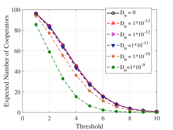
Refer to caption
Figure 12: Expected number of cooperative bacteria versus detection threshold for different diffusion coefficients of mobile bacteria Dbsubscript𝐷𝑏D_{b}. R1=50μmsubscript𝑅150𝜇mR_{1}=50\,{\mu}\textnormal{m}, expected number of bacteria is 100, and other parameters are the same as those in Section VI.

In Fig. 12, we plot expected number of cooperative bacteria versus detection threshold for different diffusion coefficients of mobile bacteria Dbsubscript𝐷𝑏D_{b}. We see that the expected number of cooperative bacteria decreases as the diffusion coefficient increases (i.e., bacteria move faster), which meets the Reviewer’s expectation (i.e., the cooperation probability is less). This is because when bacteria move faster, the average distance between bacteria is larger and fewer molecules are observed, which leads to a smaller cooperation probability and fewer cooperators. We also see that in comparison to the non-mobile case (i.e., Db=0subscript𝐷𝑏0D_{b}=0), the impact of increasing Dbsubscript𝐷𝑏D_{b} on reducing the number of cooperators is not linear. For example, increasing Dbsubscript𝐷𝑏D_{b} from 0 to Db=1011subscript𝐷𝑏superscript1011D_{b}=10^{-11} leads to a negligible drop in the number of cooperators, while increasing Dbsubscript𝐷𝑏D_{b} from Db=1011subscript𝐷𝑏superscript1011D_{b}=10^{-11} to Db=109subscript𝐷𝑏superscript109D_{b}=10^{-9} leads to 66%percent6666\% drop of the number of cooperators when the threshold at η=4𝜂4\eta=4. These values may be large for bacteria to diffuse as they are on the order of what we expect for small molecules in water. Though perhaps bacteria can “diffuse” this fast via more active means, e.g., via chemotaxis.

References

  • [1] Y. Fang, A. Noel, A. W. Eckford, and N. Yang, “Expected density of cooperative bacteria in a 2D quorum sensing based molecular communication system,” in Proc. IEEE GLOBECOM, Dec. 2019, pp. 1–7.
  • [2] J. Boedicker and K. Nealson, “Microbial communication via quorum sensing,” IEEE Trans. Mol. Bio. Multi-Scale Commun., vol. 1, no. 4, pp. 310–320, Dec. 2015.
  • [3] T. Czárán and R. F. Hoekstra, “Microbial communication, cooperation and cheating: Quorum sensing drives the evolution of cooperation in bacteria,” PLOS ONE, vol. 4, no. 8, pp. 1–10, Aug. 2009.
  • [4] S. A. West, A. S. Griffin, and A. Gardner, “Social semantics: Altruism, cooperation, mutualism, strong reciprocity and group selection,” J. Evol. Bio., vol. 20, no. 2, pp. 415–432, Mar. 2007.
  • [5] R. J. Lindsay, B. J. Pawlowska, and I. Gudelj, “When increasing population density can promote the evolution of metabolic cooperation,” The ISME J., vol. 12, pp. 849–859, Jan. 2017.
  • [6] A. Noel, Y. Fang, N. Yang, D. Makrakis, and A. W. Eckford, “Effect of local population uncertainty on cooperation in bacteria,” in Proc. IEEE ITW, Nov. 2017, pp. 334–338.
  • [7] L. Canzian, K. Zhao, G. C. L. Wong, and M. van der Schaar, “A dynamic network formation model for understanding bacterial self-organization into micro-colonies,” IEEE Trans. Mol. Bio. Multi-Scale Commun., vol. 1, no. 1, pp. 76–89, Mar. 2015.
  • [8] C. Koca and O. B. Akan, “Anarchy versus cooperation on internet of molecular things,” IEEE Internet Things J., vol. 4, no. 5, pp. 1445–1453, Oct. 2017.
  • [9] M. M. Vasconcelos, U. Mitra, O. Camara, K. P. Silva, and J. Boedicker, “Bacterial quorum sensing as a networked decision system,” in Proc. IEEE ICC, May 2018, pp. 1–6.
  • [10] N. Michelusi, J. Boedicker, M. Y. El-Naggar, and U. Mitra, “Queuing models for abstracting interactions in bacterial communities,” IEEE J. Select. Areas Commun., vol. 34, no. 3, pp. 584–599, Mar. 2016.
  • [11] B. D. Unluturk, S. Balasubramaniam, and I. F. Akyildiz, “The impact of social behavior on the attenuation and delay of bacterial nanonetworks,” IEEE Trans. Nanobiosci., vol. 15, no. 8, pp. 959–969, Dec. 2016.
  • [12] A. Einolghozati, M. Sardari, and F. Fekri, “Design and analysis of wireless communication systems using diffusion-based molecular communication among bacteria,” IEEE Trans. Wireless Commun., vol. 12, no. 12, pp. 6096–6105, Dec. 2013.
  • [13] F. Baccelli and B. Blaszczyszyn, Stochastic Geometry and Wireless Networks in Foundations and Trends in Networking, 2010.
  • [14] M. Haenggi, J. G. Andrews, F. Baccelli, O. Dousse, and M. Franceschetti, “Stochastic geometry and random graphs for the analysis and design of wireless networks,” IEEE J. Select. Areas Commun., vol. 27, no. 7, pp. 1029–1046, Sep. 2009.
  • [15] C. Picioreanu, M. C. M. van Loosdrecht, and J. J. Heijnen, “Two-dimensional model of biofilm detachment caused by internal stress from liquid flow,” Biotechnology and Bioengineering, vol. 72, no. 2, pp. 205–218, Dec. 2000.
  • [16] S. Abadal and I. F. Akyildiz, “Bio-inspired synchronization for nanocommunication networks,” in Proc. IEEE GLOBECOM, Dec. 2011, pp. 1–5.
  • [17] I. S. Gradshteyn and I. M. Ryzhik, Table of integrals, series, and products, 7th ed.   Amsterdam, Netherlands: Elsevier/Academic Press, 2007.
  • [18] M. Haenggi and R. K. Gant, “Interference in large wireless networks,” Foundations and Trends in Networking, 2009.
  • [19] A. Noel, K. C. Cheung, and R. Schober, “A unifying model for external noise sources and isi in diffusive molecular communication,” IEEE J. Select. Areas Commun., vol. 32, no. 12, pp. 2330–2343, 2014.
  • [20] A. Etemadi, P. Azmi, H. Arjmandi, and N. Mokari, “Compound poisson noise sources in diffusion-based molecular communication,” IEEE Trans. Commun., vol. 67, no. 6, pp. 4104–4116, 2019.
  • [21] T. Danino, O. Mondragón-Palomino, L. S. Tsimring, and J. Hasty, “A synchronized quorum of genetic clocks,” Nature, vol. 463, pp. 326–330, Jan. 2010.
  • [22] A. Trovato, F. Seno, M. Zanardo, S. Alberghini, A. Tondello, and A. Squartini, “Quorum vs. diffusion sensing: A quantitative analysis of the relevance of absorbing or reflecting boundaries,” FEMS Microbiology Lett., vol. 352, no. 2, pp. 198–203, Jan. 2014.
  • [23] M. G. Surette and B. L. Bassler, “Quorum sensing in Escherichia coli and Salmonella typhimurium,” Proc. Nat. Academy Sci., vol. 95, no. 12, pp. 7046–7050, Jun. 1998.
  • [24] B. Tepekule, A. E. Pusane, H. B. Yilmaz, C. Chae, and T. Tugcu, “ISI mitigation techniques in molecular communication,” IEEE Trans. Mol. Bio. Multi-Scale Commun., vol. 1, no. 2, pp. 202–216, June 2015.
  • [25] Y. Lin, W. Lin, C. Lee, and P. Yeh, “Asynchronous threshold-based detection for quantity-type-modulated molecular communication systems,” IEEE Trans. Mol. Bio. Multi-Scale Commun., vol. 1, no. 1, pp. 37–49, March 2015.
  • [26] A. Noel, Y. Fang, N. Yang, D. Makrakis, and A. W. Eckford, “Using game theory for real-time behavioral dynamics in microscopic populations with noisy signaling,” pp. 1–10, 2019. [Online]. Available: arXiv:1711.04870
  • [27] R. Salahat, E. Salahat, A. Hakam, and T. Assaf, “A simple and efficient approximation to the modified Bessel functions and its applications to Rician fading,” in Proc. IEEE GCC, Nov 2013, pp. 351–354.
  • [28] A. Noel, K. C. Cheung, and R. Schober, “Using dimensional analysis to assess scalability and accuracy in molecular communication,” in Proc. IEEE ICC, June 2013, pp. 818–823.
  • [29] F. Francesco, “Note sur une nouvelle formule de calcul differentiel,” The Quarterly Journal of Pure and Applied Mathematics, no. 1, pp. 359–360, 1857.
  • [30] R. Hogg and A. T. Craig, Introduction to Mathematical Statistics, 6th ed.   Pearson, 2004.
  • [31] L. DeCarlo, “On the meaning and use of kurtosis,” Psychological Methods, vol. 2, pp. 292–307, 09 1997.
  • [32] S. Srinivasa and M. Haenggi, “Modeling interference in finite uniformly random networks,” in WITS 2007, June 2007, pp. 1–12.
  • [33] G. E. Dilanji, J. B. Langebrake, P. D. Leenheer, and S. J. Hagen, “Quorum activation at a distance: spatiotemporal patterns of gene regulation from diffusion of an autoinducer signal.” J. Am. Chem. Soc., vol. 134, no. 12, pp. 5618–5626, 2012.
  • [34] S. S. Andrews and D. Bray, “Stochastic simulation of chemical reactions with spatial resolution and single molecule detail,” Physical Biology, vol. 1, no. 3, pp. 135–151, Aug. 2004.
  • [35] A. Noel, K. C. Cheung, and R. Schober, “Improving receiver performance of diffusive molecular communication with enzymes,” IEEE Trans. Nanobiosci., vol. 13, no. 1, pp. 31–43, Mar. 2014.
  • [36] V. Jamali, A. Ahmadzadeh, W. Wicke, A. Noel, and R. Schober, “Channel modeling for diffusive molecular communication–a tutorial review,” Proceedings of the IEEE, vol. 107, no. 7, pp. 1256–1301, July 2019.
  • [37] O. M. Cloak, B. T. Solow, C. E. Briggs, C.-Y. Chen, and P. M. Fratamico, “Quorum sensing and production of autoinducer-2 in campylobacter spp., escherichia coli o157:h7, and salmonella enterica serovar typhimurium in foods,” Applied and Environmental Microbiology, vol. 68, no. 9, pp. 4666–4671, 2002.
  • [38] J. Crank, The Mathematics of Diffusion, 2nd ed.   Oxford, UK: Oxford University Press, 1975.
  • [39] M. Haenggi, Stochastic Geometry for Wireless Networks, 1st ed.   MA, NY: Cambridge University Press, 2012.
  • [40] Y. Deng, A. Noel, W. Guo, A. Nallanathan, and M. Elkashlan, “Analyzing large-scale multiuser molecular communication via 3-D stochastic geometry,” IEEE Trans. Mol. Bio. Multi-Scale Commun., vol. 3, no. 2, pp. 118–133, June 2017.
  • [41] S. M. Ross, Introduction to Probability and Statistics for Engineers and Scientists, 5th ed.   New York, NY: Academic Press, 2014.