Factorial cumulants from global baryon number conservation

Abstract

The proton, antiproton and mixed proton-antiproton factorial cumulants originating from the global conservation of baryon number are calculated analytically up to the sixth order. Our results can be directly tested in experiments.

I Introduction

Many effective models of quantum chromodynamics (QCD) predict the first-order phase transition and the associated critical end point between the hadronic matter and quark-gluon plasma Stephanov (2004); Braun-Munzinger and Wambach (2009); Braun-Munzinger et al. (2016); Bzdak et al. (2020). One of the main approaches to search for such structures in the QCD phase diagram is based on the investigation of fluctuations of, e.g., net-baryon number, net-charge or net-strangeness number Jeon and Koch (2000); Asakawa et al. (2000); Gazdzicki et al. (2004); Gorenstein et al. (2004); Stephanov (2004); Koch et al. (2005); Stephanov (2009); Cheng et al. (2009); Fu et al. (2010); Skokov et al. (2011); Stephanov (2011); Karsch and Redlich (2011); Schaefer and Wagner (2012); Chen et al. (2011); Luo et al. (2012); Zhou et al. (2012); Wang and Yang (2012); Herold et al. (2016); Luo and Xu (2017); Szymański et al. (2020); Ratti (2019) measured in relativistic heavy ion collisions, see also a recent review in Ref. Bzdak et al. (2020).

Higher-order cumulants, $\kappa_{n}$, of the multiplicity distribution can be used to quantify the properties of such fluctuations since they are proportional to the higher powers of the correlation length Stephanov (2009). However, the cumulants mix the correlation functions of different orders, and thus in experimental situations might be challenging to interpret. Also, in practice, the cumulants might be dominated by the trivial term representing the average number of particles. To avoid these difficulties, the factorial cumulants, $\hat{C}_{n}$, can be used as they represent the integrated genuine multi-particle correlation functions Botet and Ploszajczak (2002); Ling and Stephanov (2016); Bzdak et al. (2017a, 2020).

The factorial cumulants have already been successfully applied to the STAR data on net-proton fluctuations Adamczyk et al. (2014); Luo (2015); Adam et al. (2020), which unveiled rather unexpected source of strong three- and four-proton correlations in central Au+Au collisions at $\sqrt{s_{{}_{NN}}}=7.7~{}\mathrm{GeV}$ Bzdak et al. (2017a). It was later found that these correlations are consistent with a two-component (bimodal) proton multiplicity distribution Bzdak et al. (2018); Bzdak and Koch (2019), which might indicate an interesting physics or a potential issue with the experimental data.

It is known that fluctuations and correlations related to the first-order phase transition or the critical end point may be misinterpreted because of the potentially significant contributions from various effects, which in this case play a role of the background. For instance, small fluctuations of the impact parameter and thus the number of wounded nucleons Bialas et al. (1976) were studied, e.g., in Refs. Skokov et al. (2013); Braun-Munzinger et al. (2017); Bzdak et al. (2017b). This effect may lead to significant corrections, as recently shown in Ref. Adamczewski-Musch et al. (2020), where the measurement of cumulants and factorial cumulants by the HADES Collaboration was reported. Another important effect is the global (or local) baryon number conservation, see, e.g., Bzdak et al. (2013); Braun-Munzinger et al. (2017); Rogly et al. (2019); Braun-Munzinger et al. (2019); Acharya et al. (2019); Vovchenko et al. (2020). In Ref. Acharya et al. (2019) the ALICE Collaboration emphasized the importance of the global baryon conservation at the LHC energies.

In this paper we calculate the proton, antiproton, and the mixed proton-antiproton factorial cumulants up to the sixth order, assuming that the only source of correlations is the global conservation of baryon number. The factorial cumulants of the joint proton and antiproton multiplicity distribution $P(n_{p},\bar{n}_{p})$ contain more information than the cumulants of the net-proton distribution $P(n_{p}-\bar{n}_{p})$ Bzdak et al. (2017a). Our results extend the so far published results and will allow for more sophisticated tests of the global baryon conservation effects in experiments.

In the next Section, we discuss our derivation of the proton, antiproton, and mixed proton-antiproton factorial cumulants. In Section III we present the exact results up to the sixth order and discuss some relations among them. We also provide very simple approximate expressions applicable at high energies. This is followed by the numerical results in Section IV. We finish the paper with comments and a summary. In Appendixes A-D some additional formulae and derivations are given.

II Calculation

In this Section we derive analytically the factorial cumulants of proton and antiproton multiplicity distribution, originating from the global conservation of baryon number. We assume that the only source of correlations is given by the global conservation law. By $B$ we denote the conserved baryon number, $N_{b}$ and $\bar{N}_{b}$ are the event-by-event total numbers of baryons and anti-baryons, respectively, and $n_{p}$ and $\bar{n}_{p}$ are the numbers of observed protons and antiprotons in a given rapidity and/or transverse momentum interval.

The probability distribution of $n_{p}$ and $\bar{n}_{p}$ is given by

$$P(n_{p},\bar{n}_{p}) =A\sum_{N_{b}=n_{p}}^{\infty}\sum_{\bar{N}_{b}=\bar{n}_{p}}^{\infty}\delta_{N_{b}-\bar{N}_{b},B}\left[\frac{\langle N_{b}\rangle^{N_{b}}}{N_{b}!}e^{-\langle N_{b}\rangle}\right]\left[\frac{\langle\bar{N}_{b}\rangle^{\bar{N}_{b}}}{\bar{N}_{b}!}e^{-\langle\bar{N}_{b}\rangle}\right]$$ (1)

$$\times\left[\frac{N_{b}!}{n_{p}!(N_{b}-n_{p})!}p^{n_{p}}(1-p)^{N_{b}-n_{p}}\right]\left[\frac{\bar{N}_{b}!}{\bar{n}_{p}!(\bar{N}_{b}-\bar{n}_{p})!}\bar{p}^{\bar{n}_{p}}(1-\bar{p})^{\bar{N}_{b}-\bar{n}_{p}}\right],$$

where $p=\langle n_{p}\rangle/\langle N_{b}\rangle$ is the probability that the initial baryon is observed as a proton and $\bar{p}=\langle\bar{n}_{p}\rangle/\langle\bar{N}_{b}\rangle$ is the probability that the initial antibaryon is observed as an antiproton in a given acceptance region. $\langle x\rangle$ denotes an event average value of $x$. The normalization constant is:

$$A=\frac{\left(\frac{\langle\bar{N}_{b}\rangle}{\langle N_{b}\rangle}\right)^{\frac{B}{2}}e^{{}^{\left\langle N_{b}\right\rangle+\left\langle\bar{N}_{b}\right\rangle}}}{I_{B}\left(2\sqrt{\left\langle N_{b}\right\rangle\left\langle\bar{N}_{b}\right\rangle}\right)},$$ (2)

where $I_{\nu}(x)$ is a modified Bessel function of the order $\nu$. As already emphasized, our goal is to calculate the factorial cumulants assuming that the only source of correlation is given by the conservation of baryon number. Consequently, we start with $N_{b}$ and $\bar{N}_{b}$ following Poisson distributions and the multiplicities of observed protons and antiprotons are governed by binomial distributions Bzdak et al. (2020), which do not introduce any new correlations (see also footnote $3$). The global baryon conservation is obviously enforced by $\delta_{N_{b}-\bar{N}_{b},B}$. Without this term, $P(n_{p},\bar{n}_{p})$, would be given by a product of two Poisson distributions, and all the factorial cumulants would vanish. Note that Eq. (1) can be derived from a more general expression including protons, antiprotons, neutrons, and antineutrons. This is demonstrated in Appendix A.

Using Eqs. (1) and (2), it is straightforward to calculate the factorial moment generating function (a.k.a. probability generating function)

$$H(x,\bar{x})=\sum_{n_{p}=0}^{\infty}\sum_{\bar{n}_{p}=0}^{\infty}x^{n_{p}}\bar{x}^{\bar{n}_{p}}P(n_{p},\bar{n}_{p}),$$ (3)

and the factorial cumulant generating function

$$G(x,\bar{x})=\ln[H(x,\bar{x})].$$ (4)

The result is:

$$G(x,\bar{x})=\ln\left[\left(\frac{px+1-p}{\bar{p}\bar{x}+1-\bar{p}}\right)^{\frac{B}{2}}\;\frac{I_{B}\left(2\sqrt{\left\langle N_{b}\right\rangle\left\langle\bar{N}_{b}\right\rangle(px+1-p)(\bar{p}\bar{x}+1-\bar{p})}\right)}{I_{B}\left(2\sqrt{\left\langle N_{b}\right\rangle\left\langle\bar{N}_{b}\right\rangle}\right)}\right].$$ (5)

The factorial cumulants $\hat{C}^{(n,m)}$ which are the integrated (over a given acceptance region) correlation functions for (in our context) $n$ protons and $m$ antiprotons are given by

$$\hat{C}^{(n,m)}=\left.\frac{\partial^{n}}{\partial x^{n}}\frac{\partial^{m}}{\partial\bar{x}^{m}}G(x,\bar{x})\right\rvert_{x=\bar{x}=1}.$$ (6)

By definition, the factorial cumulants $\hat{C}^{(n,m)}=0$ for all $n\geq 1$, $m\geq 1$, if there are no correlations in the system Bzdak et al. (2020), i.e., if $P(n_{p},\bar{n}_{p})$ factorizes and both $n_{p}$ and $\bar{n}_{p}$ are distributed according to Poisson distributions. The global baryon number conservation, being a long-range correlation, results in non-zero $\hat{C}^{(n,m)}$. We note that the cumulants, which are usually measured in experiments, see, e.g., Adamczyk et al. (2014); Luo (2015); Adare et al. (2016); Behera (2019); Adamczyk et al. (2014); Acharya et al. (2019); Adamczewski-Musch et al. (2020); Adam et al. (2020), can be expressed by $\hat{C}^{(n,m)}$. We will discuss this issue later on. Here we only emphasize that the cumulants mix the factorial cumulants of different orders and in general, the factorial cumulants contain more information than the cumulants.

Before we present our results let us introduce additional notation:

$$z=\sqrt{\langle N_{b}\rangle\langle\bar{N}_{b}\rangle},$$ (7)

$$\langle N_{b}\rangle_{c}=z\frac{I_{B-1}(2z)}{I_{B}(2z)},\quad\langle\bar{N}_{b}\rangle_{c}=z\frac{I_{B+1}(2z)}{I_{B}(2z)},$$ (8)

$$z_{c}=\sqrt{\langle N_{b}\rangle_{c}\langle\bar{N}_{b}\rangle_{c}},$$ (9)

where $\langle N_{b}\rangle$ is the mean number of baryons (present in Eq. (1)) before the baryon number conservation is enforced, and $\langle N_{b}\rangle_{c}$ is the mean number of baryons with the conservation of baryon number (and analogously for antibaryons). The baryon number conserved averages obviously satisfy $\langle N_{b}\rangle_{c}-\langle\bar{N}_{b}\rangle_{c}=B$ (see Eq. (8) and footnote 4).

III Results

III.1 Exact formulae

In this Section we present analytic expressions for $\hat{C}^{(n,m)}$ up to the sixth order. It is natural to define:

$$\langle N\rangle_{c}=\langle N_{b}\rangle_{c}+\langle\bar{N}_{b}\rangle_{c}\,,$$ (10)

which is the total average number of baryons. To present the formulae in a more compact way we identified commonly appearing terms and denoted them as:

$$\Delta=z_{c}^{2}-z^{2}\,,$$ (11)

$$\gamma=z_{c}^{2}+\Delta\langle N\rangle_{c}\,,$$ (12)

$$\beta=\gamma(\langle N\rangle_{c}+2)+2\Delta^{2}\,,$$ (13)

where $\langle N\rangle_{c}$, $\Delta$, $\gamma$ and $\beta$ depend on $B$ and $z$ only, see Eqs. (8) and (9). The factorial cumulants read:

$$\begin{aligned} \hat{C}^{(1,0)}&=p\langle N_{b}\rangle_{c}\end{aligned}$$ (14)

$$\begin{aligned} \hat{C}^{(2,0)}&=-p^{2}\left(\langle N_{b}\rangle_{c}+\Delta\right)\end{aligned}$$ (15)

$$\begin{aligned} \hat{C}^{(1,1)}&=-p\bar{p}\Delta\end{aligned}$$ (16)

$$\begin{aligned} \hat{C}^{(3,0)}&=p^{3}\left[2!\left(\langle N_{b}\rangle_{c}+\Delta+\tfrac{1}{2}\gamma\right)\right]\end{aligned}$$ (17)

$$\begin{aligned} \hat{C}^{(2,1)}&=p^{2}\bar{p}\,\gamma\end{aligned}$$ (18)

$$\begin{aligned} \hat{C}^{(4,0)}&=-p^{4}\left[3!\left(\langle N_{b}\rangle_{c}+\Delta+\tfrac{1}{2}\gamma\right)+\beta\right]\end{aligned}$$ (19)

$$\begin{aligned} \hat{C}^{(3,1)}&=-p^{3}\bar{p}\beta\end{aligned}$$ (20)

$$\begin{aligned} \hat{C}^{(2,2)}&=-p^{2}\bar{p}^{2}\left(\beta-\gamma\right)\end{aligned}$$ (21)

$$\begin{aligned} \hat{C}^{(5,0)}&=p^{5}\left[4!\left(\langle N_{b}\rangle_{c}+\Delta+\tfrac{1}{2}\gamma\right)+(\langle N\rangle_{c}+7)\beta+6\gamma\Delta\right]\end{aligned}$$ (22)

$$\begin{aligned} \hat{C}^{(4,1)}&=p^{4}\bar{p}\left[(\langle N\rangle_{c}+3)\beta+6\gamma\Delta\right]\end{aligned}$$ (23)

$$\begin{aligned} \hat{C}^{(3,2)}&=p^{3}\bar{p}^{2}\left[(\langle N\rangle_{c}+1)\beta+6\gamma\Delta\right]\end{aligned}$$ (24)

$$\begin{aligned} \hat{C}^{(6,0)}&=-p^{6}\left[5!\left(\langle N_{b}\rangle_{c}+\Delta+\tfrac{1}{2}\gamma\right)+\left\{(\langle N\rangle_{c}+5)(\langle N\rangle_{c}+7)+12\right\}\beta+6\gamma^{2}+16\Delta^{3}\right.\\ &\left.+2\gamma\Delta(7\langle N\rangle_{c}+35)\right]\end{aligned}$$ (25)

$$\begin{aligned} \hat{C}^{(5,1)}&=-p^{5}\bar{p}\left[(\langle N\rangle_{c}+3)(\langle N\rangle_{c}+4)\beta+6\gamma^{2}+16\Delta^{3}+2\gamma\Delta(7\langle N\rangle_{c}+20)\right]\end{aligned}$$ (26)

$$\begin{aligned} \hat{C}^{(4,2)}&=-p^{4}\bar{p}^{2}\left[(\langle N\rangle_{c}+1)(\langle N\rangle_{c}+3)\beta+6\gamma^{2}+16\Delta^{3}+2\gamma\Delta(7\langle N\rangle_{c}+11)\right]\end{aligned}$$ (27)

$$\begin{aligned} \hat{C}^{(3,3)}&=-p^{3}\bar{p}^{3}\left[(\langle N\rangle_{c}+1)(\langle N\rangle_{c}+2)\beta+6\gamma^{2}+16\Delta^{3}+2\gamma\Delta(7\langle N\rangle_{c}+8)\right]\end{aligned}$$ (28)

Having $\hat{C}^{(n,m)}$, one can easily obtain $\hat{C}^{(m,n)}$:

$$\hat{C}^{(m,n)}=\hat{C}^{(n,m)}\left(p\rightarrow\bar{p},\bar{p}\rightarrow p\right)\quad\text{for}\quad n\,m\neq 0\,,$$ (29)

$$\hat{C}^{(0,n)}=\hat{C}^{(n,0)}\left(p\rightarrow\bar{p},\langle N_{b}\rangle_{c}\rightarrow\langle\bar{N}_{b}\rangle_{c}\right)\,,$$ (30)

that is, to obtain $\hat{C}^{(m,n)}$ from $\hat{C}^{(n,m)}$ with both $n$ and $m$ larger than zero, it is enough to exchange $p$ with $\bar{p}$. To obtain $\hat{C}^{(0,n)}$ from $\hat{C}^{(n,0)}$ it is also necessary to replace $\langle N_{b}\rangle_{c}$ by $\langle\bar{N}_{b}\rangle_{c}$. For example, $\hat{C}^{(0,1)}=\bar{p}\langle\bar{N}_{b}\rangle_{c}$ and $\hat{C}^{(1,2)}=p\bar{p}^{2}\gamma$.

III.2 Relations

As seen from Equations 14–28, $\hat{C}^{(n,m)}$ is proportional to $p^{n}\bar{p}^{m}$. Therefore it is natural to study the following ratios

$$\hat{R}^{(n,m)}=\frac{\hat{C}^{(n,m)}}{p^{n}\bar{p}^{m}}\,,$$ (31)

which are independent of the size of the chosen acceptance bin.

Using Equations 14–28 we find several simple relations between various $\hat{R}^{(n,m)}$:

$$\begin{aligned} \hat{R}^{(2,0)}=\hat{R}^{(1,1)}-\hat{R}^{(1,0)}\,,\end{aligned}$$ (32)

$$\begin{aligned} \hat{R}^{(3,0)}=\hat{R}^{(2,1)}-2\hat{R}^{(2,0)}\,,\end{aligned}$$ (33)

$$\begin{aligned} \hat{R}^{(4,0)}=\hat{R}^{(3,1)}-3\hat{R}^{(3,0)}\,,\end{aligned}$$ (34)

$$\begin{aligned} \hat{R}^{(5,0)}=\hat{R}^{(4,1)}-4\hat{R}^{(4,0)}\,,\end{aligned}$$ (35)

$$\begin{aligned} \hat{R}^{(6,0)}=\hat{R}^{(5,1)}-5\hat{R}^{(5,0)}\,,\end{aligned}$$ (36)

$$\begin{aligned} \hat{R}^{(3,1)}=\hat{R}^{(2,2)}-\hat{R}^{(2,1)}\,,\end{aligned}$$ (37)

$$\begin{aligned} \hat{R}^{(4,1)}=\hat{R}^{(3,2)}-2\hat{R}^{(3,1)}\,,\end{aligned}$$ (38)

$$\begin{aligned} \hat{R}^{(5,1)}=\hat{R}^{(4,2)}-3\hat{R}^{(4,1)}\,,\end{aligned}$$ (39)

$$\begin{aligned} \hat{R}^{(4,2)}=\hat{R}^{(3,3)}-\hat{R}^{(3,2)}\,,\end{aligned}$$ (40)

or in general ($n>0$ or $m>0$)

$$\hat{R}^{(n+1,m)}=\hat{R}^{(n,m+1)}-(n-m)\hat{R}^{(n,m)}\,,$$ (41)

which we verified by direct calculations up to $n+m<9$.

III.3 Approximate formulae for $B=0$

Here, we analyze in detail the special case of $B=0$, meaning the same total number of baryons and antibaryons, which characterizes large energy conditions, such as at the LHC CERN. In this case $\langle N_{b}\rangle_{c}=\langle\bar{N}_{b}\rangle_{c}$, $z_{c}=\langle N_{b}\rangle_{c}$ and $\langle N\rangle_{c}=2\langle N_{b}\rangle_{c}$. All components appearing in Equations 14–28, that is, $\langle N\rangle_{c}$, $\langle N_{b}\rangle_{c}$, $\Delta$, $\gamma$ and $\beta$ depend on $z$ only. Next, we apply to Eq. (8) the asymptotic (large argument) expansion of the modified Bessel function Abramowitz and Stegun (1972):

$$I_{\nu}(x)\sim\frac{e^{x}}{\sqrt{2\pi x}}\left(1+\sum_{n=1}^{\infty}\frac{(-1)^{n}\prod_{i=1}^{n}(4\nu^{2}-(2i-1)^{2})}{n!(8x)^{n}}\right).$$ (42)

After eliminating the Bessel functions (the higher the order of the factorial cumulant, the more terms are needed in Eq. (42)) we expand $\hat{R}^{(n,m)}(z)$ into a power series for large $z$ and obtain the dependency of the form

$$\hat{R}^{(n,m)}(z)\sim a_{1}z+a_{0}+a_{-1}z^{-1}+a_{-2}z^{-2}+...\,,$$ (43)

where the coefficients $a_{i}$ depend on $n$ and $m$. It is worth noting that $\hat{R}^{(n,m)}(z)$ grows linearly with $z$ for large $z$. The details and explicit expressions for $\hat{R}^{(n,m)}(z)$ are presented in Appendix B.

It can be proved (see Appendix B) that $\hat{R}^{(n,m)}(z_{c})$ is also of the same form, that is, the highest-order term is proportional to $z_{c}$ and the coefficients of the series can be easily calculated. The obtained asymptotic expressions for $\hat{R}^{(n,m)}(z_{c})$ at large $z_{c}$ are given below ($z_{c}=\langle N_{b}\rangle_{c}=\langle\bar{N}_{b}\rangle_{c}$):

$$\begin{aligned} \hat{R}^{(2,0)}(z_{c})\sim-\tfrac{1}{2}z_{c}+\tfrac{1}{8}+\tfrac{1}{32}z_{c}^{-1}+...\end{aligned}$$ (44)

$$\begin{aligned} \hat{R}^{(1,1)}(z_{c})\sim\tfrac{1}{2}z_{c}+\tfrac{1}{8}+\tfrac{1}{32}z_{c}^{-1}+...\end{aligned}$$ (45)

$$\begin{aligned} \hat{R}^{(3,0)}(z_{c})\sim\tfrac{3}{4}z_{c}-\tfrac{5}{16}-\tfrac{3}{32}z_{c}^{-1}+...\end{aligned}$$ (46)

$$\begin{aligned} \hat{R}^{(2,1)}(z_{c})\sim-\tfrac{1}{4}z_{c}-\tfrac{1}{16}-\tfrac{1}{32}z_{c}^{-1}+...\end{aligned}$$ (47)

$$\begin{aligned} \hat{R}^{(4,0)}(z_{c})\sim-\tfrac{15}{8}z_{c}+\tfrac{33}{32}+\tfrac{45}{128}z_{c}^{-1}+...\end{aligned}$$ (48)

$$\begin{aligned} \hat{R}^{(3,1)}(z_{c})\sim\tfrac{3}{8}z_{c}+\tfrac{3}{32}+\tfrac{9}{128}z_{c}^{-1}+...\end{aligned}$$ (49)

$$\begin{aligned} \hat{R}^{(2,2)}(z_{c})\sim\tfrac{1}{8}z_{c}+\tfrac{1}{32}+\tfrac{5}{128}z_{c}^{-1}+...\end{aligned}$$ (50)

$$\begin{aligned} \hat{R}^{(5,0)}(z_{c})\sim\tfrac{105}{16}z_{c}-\tfrac{279}{64}-\tfrac{105}{64}z_{c}^{-1}+...\end{aligned}$$ (51)

$$\begin{aligned} \hat{R}^{(4,1)}(z_{c})\sim-\tfrac{15}{16}z_{c}-\tfrac{15}{64}-\tfrac{15}{64}z_{c}^{-1}+...\end{aligned}$$ (52)

$$\begin{aligned} \hat{R}^{(3,2)}(z_{c})\sim-\tfrac{3}{16}z_{c}-\tfrac{3}{64}-\tfrac{3}{32}z_{c}^{-1}+...\end{aligned}$$ (53)

$$\begin{aligned} \hat{R}^{(6,0)}(z_{c})\sim-\tfrac{945}{32}z_{c}+\tfrac{2895}{128}+\tfrac{4725}{512}z_{c}^{-1}+...\end{aligned}$$ (54)

$$\begin{aligned} \hat{R}^{(5,1)}(z_{c})\sim\tfrac{105}{32}z_{c}+\tfrac{105}{128}+\tfrac{525}{512}z_{c}^{-1}+...\end{aligned}$$ (55)

$$\begin{aligned} \hat{R}^{(4,2)}(z_{c})\sim\tfrac{15}{32}z_{c}+\tfrac{15}{128}+\tfrac{165}{512}z_{c}^{-1}+...\end{aligned}$$ (56)

$$\begin{aligned} \hat{R}^{(3,3)}(z_{c})\sim\tfrac{9}{32}z_{c}+\tfrac{9}{128}+\tfrac{117}{512}z_{c}^{-1}+...\end{aligned}$$ (57)

We checked, see Section IV, that the obtained approximate formulae work with very good accuracy already from $z_{c}=\langle N_{b}\rangle_{c}>2$.

IV Numerical results

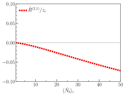
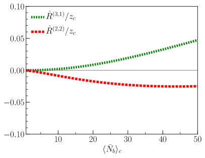
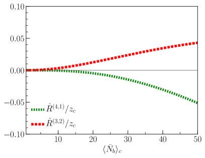
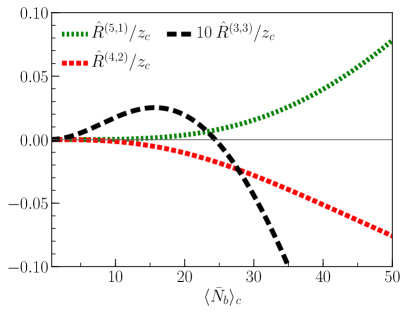
In this Section we present numerical results for $\hat{R}^{(n,m)}(z_{c})=\hat{C}^{(n,m)}/(p^{n}\bar{p}^{m})$ for two special cases: $B=0$ corresponding to large energies, and $B=300$ corresponding to central collisions at low energies in heavy-ion collisions.

IV.1 $B=0$

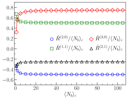
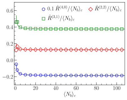
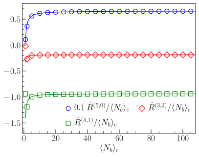
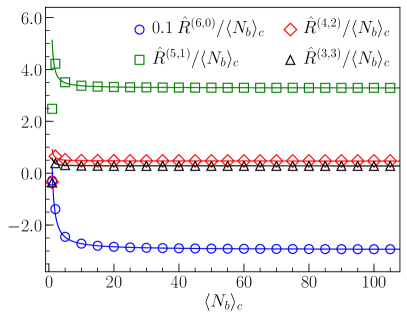
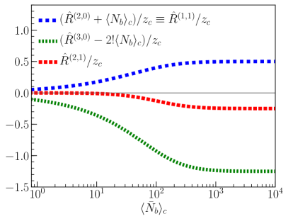
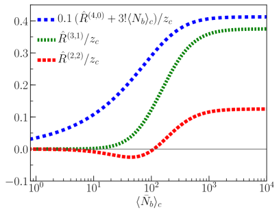
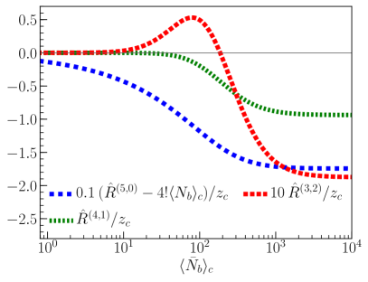
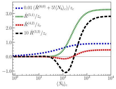
For $B=0$, $z_{c}=\langle N_{b}\rangle_{c}=\langle\bar{N}_{b}\rangle_{c}=\langle N\rangle_{c}/2$ and therefore $\hat{R}^{(n,m)}(z_{c})$ equals $\hat{R}^{(n,m)}(\langle N_{b}\rangle_{c})$. From Equations 44–57 it is clear that the dominant contribution is linear with $z_{c}=\langle N_{b}\rangle_{c}$ and there are certain deviations for small $\langle N_{b}\rangle_{c}$. Therefore, for $B=0$, it is natural to divide $\hat{R}^{(n,m)}$ by $\langle N_{b}\rangle_{c}$ so that the leading term is simply constant. In Fig. 1 we present $\hat{R}^{(n,m)}(\langle N_{b}\rangle_{c})$ divided by $\langle N_{b}\rangle_{c}$ for all the discussed factorial cumulants. Markers represent exact formulae for the factorial cumulants $\hat{C}^{(n,m)}$ given by Equations 14–28, whereas lines represent our asymptotic expressions (large $\langle N_{b}\rangle_{c}$) given by Equations 44–57. These functions are essentially constant, in agreement with our asymptotic results, except for small values of $\langle N_{b}\rangle_{c}$. The approximated formulae work very well starting from $\langle N_{b}\rangle_{c}\approx 2$. The precision better than 1% is obtained starting from $\langle N_{b}\rangle_{c}\approx 7$ in the worst case of the sixth order factorial cumulants.

Figure 1: $\hat{R}^{(n,m)}/\langle N_{b}\rangle_{c}$ as a function of $\langle N_{b}\rangle_{c}$ for $B=0$, where $\hat{R}^{(n,m)}=\hat{C}^{(n,m)}/(p^{n}\bar{p}^{m})$. Markers represent exact formulae for the factorial cumulants $\hat{C}^{(n,m)}$ given by Equations 14–28, whereas lines represent our asymptotic formulae (large $\langle N_{b}\rangle_{c}$) given by Equations 44–57. Markers are plotted for $\langle N_{b}\rangle_{c}$ = 1, 2, 5, 10, 15, …. For $\langle N_{b}\rangle_{c}>2$ the approximated formulae work very well, achieving precision better than 1% starting from $\langle N_{b}\rangle_{c}$ between 2 and 7 depending on the order of the factorial cumulant. Some of the functions were scaled by a factor of 0.1 to improve readability.

IV.2 $B=300$

Here we investigate the case of $B\neq 0$ and, as an example, we choose $B=300$. In this case, obviously $\langle N_{b}\rangle_{c}=\langle\bar{N}_{b}\rangle_{c}+B$ and now $z_{c}=[\langle N_{b}\rangle_{c}(\langle N_{b}\rangle_{c}-B)]^{1/2}$. In general $\hat{R}^{(n,m)}$ is more complicated than for $B=0$ and only for very large $z_{c}$ or $\langle N_{b}\rangle_{c}$ it asymptotically approaches a linear function. This is demonstrated in Fig. 2, where we plot $\hat{R}^{(n,m)}$ divided by $z_{c}$ as a function of $\langle\bar{N}_{b}\rangle_{c}$. We were unable to obtain a simple approximated formula and thus in Fig. 2 we present only exact $\hat{R}^{(n,m)}/z_{c}$ based on Equations 14–28. In the case of $B\neq 0$, $\hat{R}^{(n,0)}\neq\hat{R}^{(0,n)}$ and we decided to plot $(\hat{R}^{(n,0)}-(-1)^{n-1}(n-1)!\langle N_{b}\rangle_{c})/z_{c}$ because this is symmetric when baryons and antibaryons are exchanged, see Equations 14–28. We note that for some $\hat{R}^{(n,m)}/z_{c}$ with $n$, $m$ close to each other (e.g., $\hat{R}^{(2,2)}$, $\hat{R}^{(3,2)}$) we observe a maximum or minimum at $\langle\bar{N}_{b}\rangle_{c}$ about 100. Experimentally available cases at heavy-ion colliders cover the values of $\langle\bar{N}_{b}\rangle_{c}$ of the order of 100 and in Fig. 3 we show the results (except $\hat{R}^{(n,0)}$) in the range of $0<\langle\bar{N}_{b}\rangle_{c}<50$.

Figure 2: $\hat{R}^{(n,m)}/z_{c}$ as a function of $\langle\bar{N}_{b}\rangle_{c}$ for $B=300$ based on Equations 14–28. $\hat{R}^{(n,m)}=\hat{C}^{(n,m)}/(p^{n}\bar{p}^{m})$. For $m=0$ we present $(\hat{R}^{(n,0)}-(-1)^{n-1}(n-1)!\langle N_{b}\rangle_{c})/z_{c}$ because it gives the same values for both $\hat{R}^{(n,0)}$ and $\hat{R}^{(0,n)}$. Some of the functions were scaled by a factor of 10, 0.1 or 0.01 to improve readability. Note the logarithmic scale on the horizontal axis.

V Comments and summary

In this paper we calculated the proton, antiproton and mixed proton-antiproton factorial cumulants, $\hat{C}^{(n,m)}$, up to the sixth order, $n+m=6$, assuming that the only source of correlations is the global conservation of baryon number. The exact formulae are given in Equations 14–28 and for the case of $B=0$ the asymptotic expressions are provided in Equations 44–57. The latter ones represent very good approximation already from $\langle N_{b}\rangle_{c}\approx 2$.

Figure 3: Same as Fig. 2 but for $nm\neq 0$ and for small $\langle\bar{N}_{b}\rangle_{c}$. Note the linear scale on the horizontal axis. $\hat{R}^{(3,3)}/z_{c}$ was scaled by 10 to make the maximum at $\langle\bar{N}_{b}\rangle_{c}\approx 15$ visible.

Several comments are in order.

Recently the ALICE Collaboration measured Acharya et al. (2019) the second-order cumulant, $\kappa_{2}$, of the net-proton number and the result is consistent with the global baryon conservation. We note that, e.g., $\kappa_{2}$ contains less information than the second-order factorial cumulants $\hat{C}^{(2,0)}$, $\hat{C}^{(1,1)}$ and $\hat{C}^{(0,2)}$. It would be instructive to see whether the second-order factorial cumulants are consistent with the ALICE data. Also, the measurement of the higher-order factorial cumulants would be warranted.

Having all the factorial cumulants we can immediately calculate the net-proton cumulants $\kappa_{n}$. For example Bzdak et al. (2017a)

$$\kappa_{2}=\hat{C}^{(1,0)}+\hat{C}^{(0,1)}+\hat{C}^{(2,0)}+\hat{C}^{(0,2)}-2\hat{C}^{(1,1)},$$ (58)

and the expressions for the higher order $\kappa_{n}$ are shown in Appendix C. Here $\hat{C}^{(1,0)}$ and $\hat{C}^{(0,1)}$ are the mean numbers of observed, e.g., protons and antiprotons, respectively.

Finally, one possible way to measure factorial cumulants $\hat{C}^{(n,m)}$ is to first measure factorial moments $F_{i,k}\equiv\langle\frac{n!}{(n-i)!}\frac{\bar{n}!}{(\bar{n}-k)!}\rangle$, which allow to directly obtain $\hat{C}^{(n,m)}$. Explicit relations between $\hat{C}^{(n,m)}$ and $F_{i,k}$ are given in Appendix D.

Appendix A A comment on Eq. (1)

Let in each heavy-ion collision event $B=N_{p}+N_{n}-\bar{N}_{p}-\bar{N}_{n}$ be the net-baryon number. Here $N_{p}$ and $\bar{N}_{p}$ are the total numbers of protons and antiprotons, respectively, $N_{n}$ and $\bar{N}_{n}$ are the total numbers of neutrons and antineutrons. Moreover, by $n_{p}$ and $\bar{n}_{p}$ we denote the numbers of observed protons and antiprotons in a given acceptance bin. $p_{1}=\langle n_{p}\rangle/\langle N_{p}\rangle$ is the probability to observe a proton in a given acceptance region and $p_{2}=\langle\bar{n}_{p}\rangle/\langle\bar{N}_{p}\rangle$ is the probability to observe an antiproton. The probability distribution of $n_{p}$ and $\bar{n}_{p}$ is given by

$$P({n}_{p},\bar{n}_{p}) =A\sum_{N_{p}={n}_{p}}^{\infty}\sum_{\bar{N}_{p}=\bar{n}_{p}}^{\infty}\sum_{N_{n}=0}^{\infty}\sum_{\bar{N}_{n}=0}^{\infty}\delta_{N_{p}+N_{n}-\bar{N}_{p}-\bar{N}_{n},B}\left[\frac{\langle N_{p}\rangle^{N_{p}}}{N_{p}!}e^{-\langle N_{p}\rangle}\right]\left[\frac{\langle\bar{N}_{p}\rangle^{\bar{N}_{p}}}{\bar{N}_{p}!}e^{-\langle\bar{N}_{p}\rangle}\right]$$ (59)

$$\times\left[\frac{\langle N_{n}\rangle^{N_{n}}}{N_{n}!}e^{-\langle N_{n}\rangle}\right]\left[\frac{\langle\bar{N}_{n}\rangle^{\bar{N}_{n}}}{\bar{N}_{n}!}e^{-\langle\bar{N}_{n}\rangle}\right]$$

$$\times\left[\frac{N_{p}!}{{n}_{p}!(N_{p}-{n}_{p})!}p_{1}^{{n}_{p}}(1-p_{1})^{N_{p}-{n}_{p}}\right]\left[\frac{\bar{N}_{p}!}{\bar{n}_{p}!(\bar{N}_{p}-\bar{n}_{p})!}p_{2}^{\bar{n}_{p}}(1-p_{2})^{\bar{N}_{p}-\bar{n}_{p}}\right],$$

where $A$ is a normalization factor. In this expression we assume that the only source of correlation is given by the global conservation of baryon number implemented by $\delta_{N_{p}+N_{n}-\bar{N}_{p}-\bar{N}_{n},B}$.

Next, $N_{b}=N_{p}+N_{n}$ is the total number of baryons, and $\bar{N}_{b}=\bar{N}_{p}+\bar{N}_{n}$ is the total number of anti-baryons. Using relations

$$N_{p}=N_{b}-N_{n},\quad\bar{N}_{p}=\bar{N}_{b}-\bar{N}_{n}\,,$$ (60)

and summing over $N_{n}$ and $\bar{N}_{n}$ leads to our starting Eq. (1).

Appendix B Asymptotic expansion for $B=0$

Here we present more details leading to the asymptotic Equations 44–57. As already mentioned in Section III.3, in all Equations 14–28 we eliminate the Bessel functions (the higher the order of the factorial cumulant, the more terms are needed in Eq. (42) and it is enough to take the first $7$ terms for the sixth order $\hat{C}^{(n,m)}$) and expand $\hat{R}^{(n,m)}(z)$ into a power series for large $z$. We obtain:

$$\begin{aligned} \hat{R}^{(2,0)}(z)\sim-\tfrac{1}{2}z+\tfrac{1}{4}+\tfrac{3}{64}z^{-1}+...\end{aligned}$$ (61)

$$\begin{aligned} \hat{R}^{(1,1)}(z)\sim\tfrac{1}{2}z+\tfrac{1}{64}z^{-1}+...\end{aligned}$$ (62)

$$\begin{aligned} \hat{R}^{(3,0)}(z)\sim\tfrac{3}{4}z-\tfrac{1}{2}-\tfrac{15}{128}z^{-1}+...\end{aligned}$$ (63)

$$\begin{aligned} \hat{R}^{(2,1)}(z)\sim-\tfrac{1}{4}z-\tfrac{3}{128}z^{-1}+...\end{aligned}$$ (64)

$$\begin{aligned} \hat{R}^{(4,0)}(z)\sim-\tfrac{15}{8}z+\tfrac{3}{2}+\tfrac{105}{256}z^{-1}+...\end{aligned}$$ (65)

$$\begin{aligned} \hat{R}^{(3,1)}(z)\sim\tfrac{3}{8}z+\tfrac{15}{256}z^{-1}+...\end{aligned}$$ (66)

$$\begin{aligned} \hat{R}^{(2,2)}(z)\sim\tfrac{1}{8}z+\tfrac{9}{256}z^{-1}+...\end{aligned}$$ (67)

$$\begin{aligned} \hat{R}^{(5,0)}(z)\sim\tfrac{105}{16}z-6-\tfrac{945}{512}z^{-1}+...\end{aligned}$$ (68)

$$\begin{aligned} \hat{R}^{(4,1)}(z)\sim-\tfrac{15}{16}z-\tfrac{105}{512}z^{-1}+...\end{aligned}$$ (69)

$$\begin{aligned} \hat{R}^{(3,2)}(z)\sim-\tfrac{3}{16}z-\tfrac{45}{512}z^{-1}+...\end{aligned}$$ (70)

$$\begin{aligned} \hat{R}^{(6,0)}(z)\sim-\tfrac{945}{32}z+30+\tfrac{10395}{1024}z^{-1}+...\end{aligned}$$ (71)

$$\begin{aligned} \hat{R}^{(5,1)}(z)\sim\tfrac{105}{32}z+\tfrac{945}{1024}z^{-1}+...\end{aligned}$$ (72)

$$\begin{aligned} \hat{R}^{(4,2)}(z)\sim\tfrac{15}{32}z+\tfrac{315}{1024}z^{-1}+...\end{aligned}$$ (73)

$$\begin{aligned} \hat{R}^{(3,3)}(z)\sim\tfrac{9}{32}z+\tfrac{225}{1024}z^{-1}+...\end{aligned}$$ (74)

Note that all the $\hat{R}^{(n,m)}(z)$ can be written as

$$\hat{R}^{(n,m)}(z)\sim a_{1}z+a_{0}+a_{-1}z^{-1}+a_{-2}z^{-2}+...\,,$$ (75)

where the coefficients $a_{i}$ depend on $n$ and $m$ and $a_{0}\neq 0$ for $m=0$ only.

It is easy to see that $\hat{R}^{(n,m)}(z_{c})$ is also of the same form, that is, the highest term is proportional to $z_{c}$ and the coefficients of the series can be easily calculated. First, let us expand $z_{c}$ in a series of $z$:

$$z_{c}(z)\sim z-\frac{1}{4}-\frac{1}{32}z^{-1}-\frac{1}{64}z^{-2}...$$ (76)

It is clear that $\hat{R}^{(n,m)}(z_{c})$ cannot have a $z_{c}^{2}$ term (or higher order) because it would generate a $z^{2}$ term in $\hat{R}^{(n,m)}(z)$ and we know that this term is not present, see Eq. (75). Thus $\hat{R}^{(n,m)}(z_{c})$ can be written as

$$\hat{R}^{(n,m)}(z_{c})\sim b_{1}z_{c}+b_{0}+b_{-1}z_{c}^{-1}+b_{-2}z_{c}^{-2}+...\,,$$ (77)

where the coefficients $b_{i}$ are to be determined. Substituting Eq. (76) into Eq. (77) and comapring with Eq. (75) we obtain:

$$\begin{aligned} b_{1}=a_{1}\,,\end{aligned}$$ (78)

$$\begin{aligned} b_{0}=a_{0}+\tfrac{1}{4}a_{1}\,,\end{aligned}$$ (79)

$$\begin{aligned} b_{-1}=a_{-1}+\tfrac{1}{32}a_{1}\,,\end{aligned}$$ (80)

$$\begin{aligned} b_{-2}=a_{-2}-\tfrac{1}{4}a_{-1}+\tfrac{1}{128}a_{1}\,.\end{aligned}$$ (81)

Clearly, this procedure may be easily extended to obtain more terms if needed. These relations combined with Equations 61–74 lead to our Equations 44–57.

Appendix C Net-proton cumulants

The cumulant generating function for two species of particles reads

$$K(t,\bar{t})=G\left(e^{t},e^{\bar{t}}\right)\,,$$ (82)

where $G(x,\bar{x})$ is given by Eq. (4). In particular, the net-particle (e.g. net-proton) cumulants are given by ($\bar{t}=-t$)

$$\kappa_{i}=\left.\frac{d^{i}}{dt^{i}}K(t,-t)\right\rvert_{t=0}\,.$$ (83)

Combining Eqs. (82) and (83), we have:

$$\kappa_{i}=\left.\frac{d^{i}}{dt^{i}}G(x(t),\bar{x}(t))\right\rvert_{t=0}\,,$$ (84)

where $x(t)=e^{t}$ and $\bar{x}(t)=e^{-t}$ and hence derivatives $x^{(n)}(t{=}0)=1$, $\bar{x}^{(n)}(t{=}0)=(-1)^{n}$. Using this and Eq. (6), we obtain the formulae for the net-proton cumulants in terms of the factorial cumulants:

$$\begin{aligned} \kappa_{1}=\hat{C}^{(1,0)}-\hat{C}^{(0,1)}\,,\end{aligned}$$ (85)

$$\begin{aligned} \kappa_{2}=\hat{C}^{(1,0)}+\hat{C}^{(0,1)}+\hat{C}^{(2,0)}+\hat{C}^{(0,2)}-2\hat{C}^{(1,1)}\,,\end{aligned}$$ (86)

$$\begin{aligned} \kappa_{3}=\hat{C}^{(1,0)}-\hat{C}^{(0,1)}+3\left(\hat{C}^{(2,0)}-\hat{C}^{(0,2)}\right)+\hat{C}^{(3,0)}-\hat{C}^{(0,3)}-3\left(\hat{C}^{(2,1)}-\hat{C}^{(1,2)}\right)\,,\end{aligned}$$ (87)

$$\begin{aligned} \kappa_{4}&=\hat{C}^{(1,0)}+\hat{C}^{(0,1)}+7\left(\hat{C}^{(2,0)}+\hat{C}^{(0,2)}\right)-2\hat{C}^{(1,1)}+6\left(\hat{C}^{(3,0)}+\hat{C}^{(0,3)}\right)-6\left(\hat{C}^{(2,1)}+\hat{C}^{(1,2)}\right)\\ &+\hat{C}^{(4,0)}+\hat{C}^{(0,4)}-4\left(\hat{C}^{(3,1)}+\hat{C}^{(1,3)}\right)+6\hat{C}^{(2,2)}\,,\end{aligned}$$ (88)

$$\begin{aligned} \kappa_{5}&=\hat{C}^{(1,0)}-\hat{C}^{(0,1)}+15\left(\hat{C}^{(2,0)}-\hat{C}^{(0,2)}\right)+25\left(\hat{C}^{(3,0)}-\hat{C}^{(0,3)}\right)-15\left(\hat{C}^{(2,1)}-\hat{C}^{(1,2)}\right)\\ &+10\left(\hat{C}^{(4,0)}-\hat{C}^{(0,4)}\right)-20\left(\hat{C}^{(3,1)}-\hat{C}^{(1,3)}\right)+\hat{C}^{(5,0)}-\hat{C}^{(0,5)}-5\left(\hat{C}^{(4,1)}-\hat{C}^{(1,4)}\right)\\ &+10\left(\hat{C}^{(3,2)}-\hat{C}^{(2,3)}\right)\,,\end{aligned}$$ (89)

$$\begin{aligned} \kappa_{6}&=\hat{C}^{(1,0)}+\hat{C}^{(0,1)}+31\left(\hat{C}^{(2,0)}+\hat{C}^{(0,2)}\right)-2\hat{C}^{(1,1)}+90\left(\hat{C}^{(3,0)}+\hat{C}^{(0,3)}\right)\\ &-30\left(\hat{C}^{(2,1)}+\hat{C}^{(1,2)}\right)+65\left(\hat{C}^{(4,0)}+\hat{C}^{(0,4)}\right)-80\left(\hat{C}^{(3,1)}+\hat{C}^{(1,3)}\right)+30\hat{C}^{(2,2)}\\ &+15\left(\hat{C}^{(5,0)}+\hat{C}^{(0,5)}\right)-45\left(\hat{C}^{(4,1)}+\hat{C}^{(1,4)}\right)+30\left(\hat{C}^{(3,2)}+\hat{C}^{(2,3)}\right)+\hat{C}^{(6,0)}+\hat{C}^{(0,6)}\\ &-6\left(\hat{C}^{(5,1)}+\hat{C}^{(1,5)}\right)+15\left(\hat{C}^{(4,2)}+\hat{C}^{(2,4)}\right)-20\hat{C}^{(3,3)}\,,\end{aligned}$$ (90)

where $\hat{C}^{(1,0)}$ and $\hat{C}^{(0,1)}$ are the mean numbers of, e.g., protons and antiprotons, respectively. These results extend the formulae provided in Appendix A of Ref. Bzdak et al. (2017a).

Appendix D $\hat{C}^{(n,m)}$ vs $F_{i,k}$

The factorial moments for two variables (two species of particles) are defined via the factorial moment generating function $H(x,\bar{x})$ (see Eq. (3)):

$$F_{i,k}\equiv\left\langle\frac{n_{1}!}{(n_{1}-i)!}\frac{n_{2}!}{(n_{2}-k)!}\right\rangle=\left.\frac{d^{i}}{dx^{i}}\frac{d^{k}}{d\bar{x}^{k}}H(x,\bar{x})\right\rvert_{x=\bar{x}=1}.$$ (91)

Using Eqs. (4) and (6), and the normalization condition $H(1,1)=1$, we can express the factorial cumulants through the factorial moments:

$$\begin{aligned} \hat{C}^{(1,0)}&=F_{1,0}\end{aligned}$$ (92)

$$\begin{aligned} \hat{C}^{(0,1)}&=F_{0,1}\end{aligned}$$ (93)

$$\begin{aligned} \hat{C}^{(2,0)}=-F_{1,0}^{2}+F_{2,0}\end{aligned}$$ (94)

$$\begin{aligned} \hat{C}^{(1,1)}=-F_{0,1}F_{1,0}+F_{1,1}\end{aligned}$$ (95)

$$\begin{aligned} \hat{C}^{(3,0)}=2F_{1,0}^{3}-3F_{1,0}F_{2,0}+F_{3,0}\end{aligned}$$ (96)

$$\begin{aligned} \hat{C}^{(2,1)}&=2F_{0,1}F_{1,0}^{2}-2F_{1,0}F_{1,1}-F_{0,1}F_{2,0}+F_{2,1}\end{aligned}$$ (97)

$$\begin{aligned} \hat{C}^{(4,0)}&=-6F_{1,0}^{4}+12F_{1,0}^{2}F_{2,0}-3F_{2,0}^{2}-4F_{1,0}F_{3,0}+F_{4,0}\end{aligned}$$ (98)

$$\begin{aligned} \hat{C}^{(3,1)}&=-6F_{0,1}F_{1,0}^{3}+6F_{1,0}^{2}F_{1,1}+6F_{0,1}F_{1,0}F_{2,0}-3F_{1,1}F_{2,0}-3F_{1,0}F_{2,1}-F_{0,1}F_{3,0}+F_{3,1}\end{aligned}$$ (99)

$$\begin{aligned} \hat{C}^{(2,2)}&=\left(-6F_{0,1}^{2}+2F_{0,2}\right)F_{1,0}^{2}+8F_{0,1}F_{1,0}F_{1,1}-2F_{1,1}^{2}-2F_{1,0}F_{1,2}+\left(2F_{0,1}^{2}-F_{0,2}\right)F_{2,0}\\ &-2F_{0,1}F_{2,1}+F_{2,2}\end{aligned}$$ (100)

$$\begin{aligned} \hat{C}^{(5,0)}&=24F_{1,0}^{5}-60F_{1,0}^{3}F_{2,0}+30F_{1,0}F_{2,0}^{2}+20F_{1,0}^{2}F_{3,0}-10F_{2,0}F_{3,0}-5F_{1,0}F_{4,0}+F_{5,0}\end{aligned}$$ (101)

$$\begin{aligned} \hat{C}^{(4,1)}&=24F_{0,1}F_{1,0}^{4}-24F_{1,0}^{3}F_{1,1}-36F_{0,1}F_{1,0}^{2}F_{2,0}+24F_{1,0}F_{1,1}F_{2,0}+6F_{0,1}F_{2,0}^{2}+12F_{1,0}^{2}F_{2,1}\\ &-6F_{2,0}F_{2,1}+8F_{0,1}F_{1,0}F_{3,0}-4F_{1,1}F_{3,0}-4F_{1,0}F_{3,1}-F_{0,1}F_{4,0}+F_{4,1}\end{aligned}$$ (102)

$$\begin{aligned} \hat{C}^{(3,2)}&=2\left(12F_{0,1}^{2}-3F_{0,2}\right)F_{1,0}^{3}-36F_{0,1}F_{1,0}^{2}F_{1,1}+12F_{1,0}F_{1,1}^{2}+6F_{1,0}^{2}F_{1,2}\\ &-3\left(6F_{0,1}^{2}-2F_{0,2}\right)F_{1,0}F_{2,0}+12\left(F_{1,1}F_{2,0}+F_{1,0}F_{2,1}\right)F_{0,1}-3F_{1,2}F_{2,0}-6F_{1,1}F_{2,1}\\ &-3F_{1,0}F_{2,2}+\left(2F_{0,1}^{2}-F_{0,2}\right)F_{3,0}-2F_{0,1}F_{3,1}+F_{3,2}\end{aligned}$$ (103)

$$\begin{aligned} \hat{C}^{(6,0)}&=-120F_{1,0}^{6}+360F_{2,0}F_{1,0}^{4}-120F_{3,0}F_{1,0}^{3}-270F_{2,0}^{2}F_{1,0}^{2}+30F_{4,0}F_{1,0}^{2}+120F_{2,0}F_{3,0}F_{1,0}\\ &-6F_{5,0}F_{1,0}+30F_{2,0}^{3}-10F_{3,0}^{2}-15F_{2,0}F_{4,0}+F_{6,0}\end{aligned}$$ (104)

$$\begin{aligned} \hat{C}^{(5,1)}&=-120F_{0,1}F_{1,0}^{5}+120F_{1,1}F_{1,0}^{4}+240F_{0,1}F_{2,0}F_{1,0}^{3}-60F_{2,1}F_{1,0}^{3}-180F_{1,1}F_{2,0}F_{1,0}^{2}\\ &-60F_{0,1}F_{3,0}F_{1,0}^{2}+20F_{3,1}F_{1,0}^{2}-90F_{0,1}F_{2,0}^{2}F_{1,0}+60F_{2,0}F_{2,1}F_{1,0}+40F_{1,1}F_{3,0}F_{1,0}\\ &+10F_{0,1}F_{4,0}F_{1,0}-5F_{4,1}F_{1,0}+30F_{1,1}F_{2,0}^{2}+20F_{0,1}F_{2,0}F_{3,0}-10F_{2,1}F_{3,0}-10F_{2,0}F_{3,1}\\ &-5F_{1,1}F_{4,0}-F_{0,1}F_{5,0}+F_{5,1}\end{aligned}$$ (105)

$$\begin{aligned} \hat{C}^{(4,2)}&=-6\left(20F_{0,1}^{2}-4F_{0,2}\right)F_{1,0}^{4}+192F_{0,1}F_{1,1}F_{1,0}^{3}+12\left(12F_{0,1}^{2}-3F_{0,2}\right)F_{2,0}F_{1,0}^{2}\\ &-4\left(6F_{0,1}^{2}-2F_{0,2}\right)F_{3,0}F_{1,0}-3\left(6F_{0,1}^{2}-2F_{0,2}\right)F_{2,0}^{2}-6\left(4F_{1,2}F_{1,0}^{3}+12F_{1,1}^{2}F_{1,0}^{2}\right)\\ &+24F_{0,1}F_{2,0}F_{2,1}-72F_{0,1}\left(F_{2,1}F_{1,0}^{2}+2F_{1,1}F_{2,0}F_{1,0}\right)\\ &+12\left(F_{2,2}F_{1,0}^{2}+4F_{1,1}F_{2,1}F_{1,0}+\left(2F_{1,1}^{2}+2F_{1,0}F_{1,2}\right)F_{2,0}\right)-3\left(2F_{2,1}^{2}+2F_{2,0}F_{2,2}\right)\\ &+16F_{0,1}\left(F_{1,1}F_{3,0}+F_{1,0}F_{3,1}\right)-4\left(F_{1,2}F_{3,0}+2F_{1,1}F_{3,1}+F_{1,0}F_{3,2}\right)\\ &+\left(2F_{0,1}^{2}-F_{0,2}\right)F_{4,0}-2F_{0,1}F_{4,1}+F_{4,2}\end{aligned}$$ (106)

$$\begin{aligned} \hat{C}^{(3,3)}&=2\left(-60F_{0,1}^{3}+36F_{0,2}F_{0,1}-3F_{0,3}\right)F_{1,0}^{3}+18\left(12F_{0,1}^{2}-3F_{0,2}\right)F_{1,1}F_{1,0}^{2}\\ &-3\left(-24F_{0,1}^{3}+18F_{0,2}F_{0,1}-2F_{0,3}\right)F_{2,0}F_{1,0}-18F_{0,1}\left(3F_{1,2}F_{1,0}^{2}+6F_{1,1}^{2}F_{1,0}\right)\\ &+2\left(6F_{1,1}^{3}+18F_{1,0}F_{1,2}F_{1,1}+3F_{1,0}^{2}F_{1,3}\right)-9\left(6F_{0,1}^{2}-2F_{0,2}\right)\left(F_{1,1}F_{2,0}+F_{1,0}F_{2,1}\right)\\ &+18F_{0,1}\left(F_{1,2}F_{2,0}+2F_{1,1}F_{2,1}+F_{1,0}F_{2,2}\right)\\ &-3\left(F_{1,3}F_{2,0}+3F_{1,2}F_{2,1}+3F_{1,1}F_{2,2}+F_{1,0}F_{2,3}\right)+\left(-6F_{0,1}^{3}+6F_{0,2}F_{0,1}-F_{0,3}\right)F_{3,0}\\ &+3\left(2F_{0,1}^{2}-F_{0,2}\right)F_{3,1}-3F_{0,1}F_{3,2}+F_{3,3}.\end{aligned}$$ (107)

These results extend the formulae provided in Appendix A of Ref. Bzdak et al. (2017a).

References

- Stephanov (2004) M. A. Stephanov, Non-perturbative quantum chromodynamics. Proceedings, 8th Workshop, Paris, France, June 7-11, 2004, Prog. Theor. Phys. Suppl. 153, 139 (2004), [Int. J. Mod. Phys.A20,4387(2005)], arXiv:hep-ph/0402115 [hep-ph] .
- Braun-Munzinger and Wambach (2009) P. Braun-Munzinger and J. Wambach, Rev. Mod. Phys. 81, 1031 (2009), arXiv:0801.4256 [hep-ph] .
- Braun-Munzinger et al. (2016) P. Braun-Munzinger, V. Koch, T. Schäfer, and J. Stachel, Phys. Rept. 621, 76 (2016), arXiv:1510.00442 [nucl-th] .
- Bzdak et al. (2020) A. Bzdak, S. Esumi, V. Koch, J. Liao, M. Stephanov, and N. Xu, Phys. Rept. 853, 1 (2020), arXiv:1906.00936 [nucl-th] .
- Jeon and Koch (2000) S. Jeon and V. Koch, Phys. Rev. Lett. 85, 2076 (2000), arXiv:hep-ph/0003168 [hep-ph] .
- Asakawa et al. (2000) M. Asakawa, U. W. Heinz, and B. Muller, Phys. Rev. Lett. 85, 2072 (2000), arXiv:hep-ph/0003169 [hep-ph] .
- Gazdzicki et al. (2004) M. Gazdzicki, M. I. Gorenstein, and S. Mrowczynski, Phys. Lett. B585, 115 (2004), arXiv:hep-ph/0304052 [hep-ph] .
- Gorenstein et al. (2004) M. I. Gorenstein, M. Gazdzicki, and O. S. Zozulya, Phys. Lett. B585, 237 (2004), arXiv:hep-ph/0309142 [hep-ph] .
- Koch et al. (2005) V. Koch, A. Majumder, and J. Randrup, Phys. Rev. Lett. 95, 182301 (2005), arXiv:nucl-th/0505052 [nucl-th] .
- Stephanov (2009) M. A. Stephanov, Phys. Rev. Lett. 102, 032301 (2009), arXiv:0809.3450 [hep-ph] .
- Cheng et al. (2009) M. Cheng et al., Phys. Rev. D79, 074505 (2009), arXiv:0811.1006 [hep-lat] .
- Fu et al. (2010) W.-j. Fu, Y.-x. Liu, and Y.-L. Wu, Phys. Rev. D81, 014028 (2010), arXiv:0910.5783 [hep-ph] .
- Skokov et al. (2011) V. Skokov, B. Friman, and K. Redlich, Phys. Rev. C83, 054904 (2011), arXiv:1008.4570 [hep-ph] .
- Stephanov (2011) M. A. Stephanov, Phys. Rev. Lett. 107, 052301 (2011), arXiv:1104.1627 [hep-ph] .
- Karsch and Redlich (2011) F. Karsch and K. Redlich, Phys. Rev. D84, 051504 (2011), arXiv:1107.1412 [hep-ph] .
- Schaefer and Wagner (2012) B. J. Schaefer and M. Wagner, Phys. Rev. D85, 034027 (2012), arXiv:1111.6871 [hep-ph] .
- Chen et al. (2011) L. Chen, X. Pan, F.-B. Xiong, L. Li, N. Li, Z. Li, G. Wang, and Y. Wu, J. Phys. G38, 115004 (2011).
- Luo et al. (2012) X.-F. Luo, B. Mohanty, H. G. Ritter, and N. Xu, Phys. Atom. Nucl. 75, 676 (2012), arXiv:1105.5049 [nucl-ex] .
- Zhou et al. (2012) D.-M. Zhou, A. Limphirat, Y.-l. Yan, C. Yun, Y.-p. Yan, X. Cai, L. P. Csernai, and B.-H. Sa, Phys. Rev. C85, 064916 (2012), arXiv:1205.5634 [nucl-th] .
- Wang and Yang (2012) X. Wang and C. B. Yang, Phys. Rev. C85, 044905 (2012), arXiv:1202.4857 [nucl-th] .
- Herold et al. (2016) C. Herold, M. Nahrgang, Y. Yan, and C. Kobdaj, Phys. Rev. C93, 021902 (2016), arXiv:1601.04839 [hep-ph] .
- Luo and Xu (2017) X. Luo and N. Xu, Nucl. Sci. Tech. 28, 112 (2017), arXiv:1701.02105 [nucl-ex] .
- Szymański et al. (2020) M. Szymański, M. Bluhm, K. Redlich, and C. Sasaki, J. Phys. G 47, 045102 (2020), arXiv:1905.00667 [nucl-th] .
- Ratti (2019) C. Ratti, PoS LATTICE2018, 004 (2019).
- Botet and Ploszajczak (2002) R. Botet and M. Ploszajczak, Universal fluctuations: The phenomenology of hadronic matter (River Edge, USA: World Scientific (2002) 369, 2002).
- Ling and Stephanov (2016) B. Ling and M. A. Stephanov, Phys. Rev. C93, 034915 (2016), arXiv:1512.09125 [nucl-th] .
- Bzdak et al. (2017a) A. Bzdak, V. Koch, and N. Strodthoff, Phys. Rev. C95, 054906 (2017a), arXiv:1607.07375 [nucl-th] .
- Adamczyk et al. (2014) L. Adamczyk et al. (STAR), Phys. Rev. Lett. 112, 032302 (2014), arXiv:1309.5681 [nucl-ex] .
- Luo (2015) X. Luo (STAR), Proceedings, 9th International Workshop on Critical Point and Onset of Deconfinement (CPOD 2014): Bielefeld, Germany, November 17-21, 2014, PoS CPOD2014, 019 (2015), arXiv:1503.02558 [nucl-ex] .
- Adam et al. (2020) J. Adam et al. (STAR), (2020), arXiv:2001.02852 [nucl-ex] .
- Bzdak et al. (2018) A. Bzdak, V. Koch, D. Oliinychenko, and J. Steinheimer, Phys. Rev. C98, 054901 (2018), arXiv:1804.04463 [nucl-th] .
- Bzdak and Koch (2019) A. Bzdak and V. Koch, Phys. Rev. C100, 051902 (2019), arXiv:1811.04456 [nucl-th] .
- Bialas et al. (1976) A. Bialas, M. Bleszynski, and W. Czyz, Nucl. Phys. B111, 461 (1976).
- Skokov et al. (2013) V. Skokov, B. Friman, and K. Redlich, Phys. Rev. C88, 034911 (2013), arXiv:1205.4756 [hep-ph] .
- Braun-Munzinger et al. (2017) P. Braun-Munzinger, A. Rustamov, and J. Stachel, Nucl. Phys. A960, 114 (2017), arXiv:1612.00702 [nucl-th] .
- Bzdak et al. (2017b) A. Bzdak, V. Koch, and V. Skokov, Eur. Phys. J. C77, 288 (2017b), arXiv:1612.05128 [nucl-th] .
- Adamczewski-Musch et al. (2020) J. Adamczewski-Musch et al. (HADES), (2020), arXiv:2002.08701 [nucl-ex] .
- Bzdak et al. (2013) A. Bzdak, V. Koch, and V. Skokov, Phys. Rev. C87, 014901 (2013), arXiv:1203.4529 [hep-ph] .
- Rogly et al. (2019) R. Rogly, G. Giacalone, and J.-Y. Ollitrault, Phys. Rev. C 99, 034902 (2019), arXiv:1809.00648 [nucl-th] .
- Braun-Munzinger et al. (2019) P. Braun-Munzinger, A. Rustamov, and J. Stachel, (2019), arXiv:1907.03032 [nucl-th] .
- Acharya et al. (2019) S. Acharya et al. (ALICE), (2019), arXiv:1910.14396 [nucl-ex] .
- Vovchenko et al. (2020) V. Vovchenko, O. Savchuk, R. V. Poberezhnyuk, M. I. Gorenstein, and V. Koch, (2020), arXiv:2003.13905 [hep-ph] .
- Kitazawa and Asakawa (2012a) M. Kitazawa and M. Asakawa, Phys. Rev. C 85, 021901 (2012a), arXiv:1107.2755 [nucl-th] .
- Kitazawa and Asakawa (2012b) M. Kitazawa and M. Asakawa, Phys. Rev. C 86, 024904 (2012b), [Erratum: Phys.Rev.C 86, 069902 (2012)], arXiv:1205.3292 [nucl-th] .
- Adare et al. (2016) A. Adare et al. (PHENIX), Phys. Rev. C93, 011901 (2016), arXiv:1506.07834 [nucl-ex] .
- Behera (2019) N. K. Behera (ALICE), Proceedings, 27th International Conference on Ultrarelativistic Nucleus-Nucleus Collisions (Quark Matter 2018): Venice, Italy, May 14-19, 2018, Nucl. Phys. A982, 851 (2019), arXiv:1807.06780 [hep-ex] .
- Abramowitz and Stegun (1972) M. Abramowitz and I. Stegun, Handbook of Mathematical Functions With Formulas, Graphs, and Mathematical Tables (United States Department of Commerce. National Bureau of Standards. Applied Mathematics Series. Washington D.C., 1972).