One Step to Efficient Synthetic Data

Jordan Awan^∗, Zhanrui Cai^†

Purdue University^∗, Iowa State University^†

Abstract:

A common approach to synthetic data is to sample from a fitted model. We show that under general assumptions, this approach results in a sample with inefficient estimators, and the joint distribution of the sample is inconsistent with the true distribution. Motivated by this, we propose a general method of producing synthetic data that is widely applicable for parametric models, has asymptotically efficient summary statistics, and is easily implemented and highly computationally efficient. Our approach allows for the construction of both partially synthetic datasets, which preserve certain summary statistics, as well as fully synthetic data, which satisfy differential privacy. In the case of continuous random variables, we prove that our method preserves the efficient estimator with asymptotically negligible error and show through simulations that this property holds for discrete distributions as well. We also provide theoretical and empirical evidence that the distribution from our procedure converges to the true distribution. Besides our focus on synthetic data, our procedure can also be used to perform hypothesis tests in the presence of intractable likelihood functions.

Key words and phrases: indirect inference, parametric bootstrap, simulation-based inference, statistical disclosure control, differential privacy

1 Introduction

With advances in modern technology, the government and other research agencies can collect massive amounts of data from individual respondents. These data are valuable for scientific progress and policy research, but they also come with increased privacy risk (Lane et al., 2014). Numerous methods of generating synthetic data have been proposed to publish useful information while preserving the confidentiality of sensitive information. For a survey, we refer interested readers to Hundepool et al. (2012, Chapter 3). The goal of synthetic data is to produce a new dataset that preserves the distributional properties of the original dataset, while protecting the privacy of the participating individuals. There are two main types of synthetic data: partially synthetic data, which allows for certain statistics or attributes to be released without privacy while protecting the other aspects of the data, and fully synthetic data, where all statistics and attributes of the data are protected.

There has also been an increased interest in developing synthetic data with formal privacy guarantees, such as differential privacy (DP). Differential privacy (DP) was proposed in Dwork et al. (2006) as a framework to develop formally private methods. Methods that satisfy DP require the introduction of additional randomness beyond sampling to obscure the effect of one individual on the output. Intuitively, DP ensures plausible deniability for those participating in the dataset.

A common approach to synthetic data is that of Liew et al. (1985), which proposes to draw synthetic data from a fitted model, which we also refer to as the parametric bootstrap. This forms the basis of the multiple imputation method of synthetic data generation (Rubin, 1993; Raghunathan et al., 2003; Drechsler, 2011; Jiang et al., 2021). Another approach to synthetic data samples from a conditional distribution, preserving certain statistics. The most fundamental perspective of this approach is that of Muralidhar and Sarathy (2003), who proposes drawing confidential variables from the distribution conditional on the non-confidential variables.

Our contributions Related work on synthetic data largely fits into one of two categories: 1) sampling from a fitted distribution or 2) sampling from a distribution conditional on sample statistics. Our first result, Theorem 2 shows that in very general settings, the first approach results in a sample with inefficient estimators, and whose distribution is “inconsistent.” In particular, we show that the joint distribution of the synthetic sample does not converge in total variation to the true joint distribution as the sample size increases. This result gives a strong indication that the parametric bootstrap is not ideal for synthetic data generation. On the other hand, sampling conditional on certain sample statistics can overcome these issues.

However, there are important limitations to the previous works which sample from a conditional distribution. First, the previous approaches are all highly specific to the model at hand and require different techniques for different models. Second, many of the approaches are difficult to implement and computationally expensive, involving complex iterative sampling schemes such as MCMC.

The approach we propose in this paper preserves summary statistics, but unlike previous methods it is applicable to a wide variety of parametric models, easily implemented, and highly computationally efficient. Our approach allows for the construction of both partially synthetic datasets, which preserve the summary statistics without formal privacy methods, as well as fully synthetic data which satisfy the strong guarantee of differential privacy (DP).

Our contributions are summarized as follows:

• We prove that the parametric bootstrap results in inconsistent synthetic data with inefficient estimators.

• We propose a novel method, “one-step synthetic data,” which adds one extra step to the parametric bootstrap. Our approach is easily applied as the computations only require efficient estimators for the parameters and the ability to sample the model, and the computational time is proportional to simply fitting the model.

• We prove that under regularity conditions that our synthetic data procedure preserves an efficient estimator with an asymptotically negligible error. We call this “efficient synthetic data,” as its estimators are also efficient.

• We prove that when conditioning on an efficient estimator, the distributions still converge even if the parameters differ by $O(n^{-1/2})$. We argue that our method is an approximation to a conditional distribution and this gives evidence that the one-step synthetic data asymptotically has the same distribution as the original dataset.

• We investigate the performance of our procedure in several simulation studies, confirming the theoretical results, and offering numerical evidence that the assumptions can likely be weakened.

Organization The rest of the paper is organized as follows: In Section 2, we review some terminology and set the notation for the paper. In Section 3, we prove the limitations of synthetic data generated by the parametric bootstrap, showing that the distribution is inconsistent and has inefficient summary statistics. We propose our one-step approach to synthetic data in Section 4 and in the case of continuous random variables, prove that it results in a sample which preserves an efficient estimator with asymptotically negligible error. In Section 5, we consider the distribution of the one-step synthetic sample, and prove that a related procedure results in a consistent sample, giving evidence that the one-step procedure itself is consistent. In Section 6 we perform several simulation studies illustrating 1) the efficiency of the one-step synthetic data estimators, even in the case of discrete distributions, 2) the distributional properties of the approach, 3) that the approach can give high quality DP synthetic data, and 4) the one-step synthetic data can perform accurate and powerful hypothesis tests on models with intractible likelihood functions. We end in Section 7 with some discussion. Proofs and technical details are postponed to Section S3 of the Supplementary Materials.

Related work The approach of sampling from a fitted model is often used to produce differentially private synthetic data. Hall et al. (2013) develop DP tools for kernel density estimators, which can be sampled to produce DP synthetic data. Machanavajjhala et al. (2008) develop a synthetic data method based on a multinomial model, which satisfies a modified version of DP to accommodate sparse spatial data. McClure and Reiter (2012) sample from the posterior predictive distribution to produce DP synthetic data, which is asymptotically similar to the Liew et al. (1985). Liu (2016) also use a Bayesian framework: first, they produce DP estimates of the Bayesian sufficient statistics, draw the parameter from the distribution conditional on the DP statistics, and finally sample synthetic data conditional on the sampled parameter. Zhang et al. (2017) propose a method of developing high-dimensional DP synthetic data which draws from a fitted model based on differentially private marginals. While not for the purpose of generating synthetic data, Ferrando et al. (2022) proposed using the parametric bootstrap to do statistical inference on model parameters, given privatized statistics.

Burridge (2003); Mateo-Sanz et al. (2004); Ting et al. (2005) generate partially synthetic data, preserving the mean and covariance for normally distributed variables. There are also tools, often based on algebraic statistics, to sample conditional distributions preserving certain statistics for contingency tables (Karwa and Slavković, 2013; Chen et al., 2006; Slavković and Lee, 2010).

While not focused on the problem of synthetic data, there are other notable works sampling from conditional distributions. A series of works sample from distributions conditional on sufficient statistics focused on the application of hypothesis testing (Lindqvist and Taraldsen, 2005, 2007, 2013; Lillegard and Engen, 1999; Engen and Lillegård, 1997; Lillegard and Engen, 1999; Taraldsen and Lindqvist, 2018). Barber and Janson (2022) recently gave a method of sampling conditional on an efficient statistic using the principle of asymptotic sufficiency; they showed that their method results in asymptotically valid $p$-values for certain hypothesis tests.

In differential privacy, synthetic data methods also preserve sample statistics. Karwa and Slavković (2012) generate DP synthetic networks from the beta exponential random graph model, conditional on the degree sequence. Li et al. (2018) produce DP high dimensional synthetic contingency tables using a modified Gibbs sampler. Hardt et al. (2012) give a distribution-free algorithm to produce a DP synthetic dataset, which approximately preserves several linear statistics.

While this paper is focused on producing synthetic data for parametric models, there are several non-parametric methods of producing synthetic data, using tools such as regression trees (Reiter, 2005; Drechsler and Reiter, 2008), random forests (Caiola and Reiter, 2010), bagging and support vector machines (Drechsler and Reiter, 2011). Recently there has been a success in producing differentially privacy synthetic data using generative adversarial neural networks (Xie et al., 2018; Jordon et al., 2018; Triastcyn and Faltings, 2018; Xu et al., 2019; Harder et al., 2021). We also mention a hardness result due to Ullman and Vadhan (2020), which establishes that there is no polynomial time algorithm which can approximately preserve all two-way margins of binary data; our focus on parametric models side-steps this issue.

2 Background and notation

In this section, we review some background and notation that we use throughout the paper.

For a parametric random variable, we write $X\sim f_{\theta}$ to indicate that $X$ has probability density function (pdf) $f_{\theta}$. To indicate that a sequence of random variables from the model $f_{\theta}$ are independent and identically distributed (i.i.d.), we write $X_{1},\ldots,X_{n}\overset{\text{i.i.d.}}{\sim}f_{\theta}$, and denote $f_{\theta}^{n}$ as the joint pdf of $(X_{1},\ldots,X_{n})$. We use all of the following notations interchangeably: $\underline{X}=(X_{i})_{i=1}^{n}=(X_{1},\ldots,X_{n})^{\top}$. We write $\mathbb{R}^{d\times n}$ to denote the set of all $n$-tuples of elements from $\mathbb{R}^{d}$.

Our notation for convergence of random variables follows that of Van der Vaart (2000). Let $X$ be a random vector, $X_{n}$ be a sequence of random vectors, and $r_{n}$ be a positive numerical sequence. We write $X_{n}\overset{d}{\rightarrow}X$ to denote that $X_{n}$ converges in distribution to $X$. We write $X_{n}=o_{p}(r_{n})$ to denote that $X_{n}/r_{n}\overset{d}{\rightarrow}0$. We write $X_{n}=O_{p}(r_{n})$ to denote that $X_{n}/r_{n}$ is bounded in probability.

For $X\sim f_{\theta}$, we denote the score function as $S(\theta,x)=\nabla_{\theta}\log f_{\theta}(x)$, and the Fisher Information as $I(\theta)=E_{\theta}\left[S(\theta,X)S^{\top}(\theta,X)\right]$, where $E_{\theta}$ denotes the expectation over the random variable $X$ when $\theta$ is the true parameter. An estimator $\hat{\theta}:\mathbb{R}^{d\times n}\rightarrow\Theta$ is efficient if for $X_{1},\ldots,X_{n}\overset{\text{i.i.d.}}{\sim}f_{\theta}$, we have $\sqrt{n}(\hat{\theta}(\underline{X})-\theta)\overset{d}{\rightarrow}N(0,I^{-1}(\theta))$. We will often write ${\hat{\theta}_{X}}$ in place of $\hat{\theta}(\underline{X})$.

3 Limitations of the parametric bootstrap for synthetic data

Sampling from a fitted model, also known as the parametric bootstrap, is a common approach to synthetic data. However, the parametric bootstrap has considerable weaknesses when used to generate synthetic data, in that it results in significantly worse approximations to the true sampling distribution. In this section, we prove that the parametric bootstrap gives inefficient sample statistics and results in “inconsistent” synthetic data, where we show that the total variation distance between the true distribution and the parametric bootstrap approximation does not go to zero as $n\rightarrow\infty$.

Our goal in this paper is to produce a new dataset $\underline{Y}$ which is approximately equal in distribution to $\underline{X}$, where the approximation is measured by total variation distance, $\mathrm{TV}(\underline{X},\underline{Y})$. At a minimum, we may expect that the distribution of $\underline{Y}$ approaches the distribution of $\underline{X}$ as the sample size $n$ grows. We begin with an example that shows that the parametric bootstrap results in suboptimal asymptotics, calling into question the appropriateness of the parametric bootstrap for the generation of synthetic data.

Example 1.

Suppose that $X_{1}\ldots,X_{n}\overset{\text{i.i.d.}}{\sim}N(\mu,1)$. We use the estimator $\hat{\mu}(\underline{X})=n^{-1}\sum_{i=1}^{n}X_{i}$ and draw $Z_{1},\ldots,Z_{n}|\hat{\mu}(\underline{X})\overset{\text{i.i.d.}}{\sim}N\{\hat{\mu}(\underline{X}),1\}$. We can compute $\operatorname{Var}(\hat{\mu}(\underline{X}))=n^{-1}$, whereas $\operatorname{Var}\{\hat{\mu}(\underline{Z})\}=2n^{-1}$. By using the synthetic data $\underline{Z}$, we have lost half of the effective sample size. We can also derive $(Z_{1},\ldots,Z_{n})^{\top}\sim N(\mu\underline{1},I_{n}+n^{-1}\underline{1}\,\underline{1}^{\top})$, where $\underline{1}=(1,\ldots,1)^{\top}$ is a vector of length $n$. Using the formula for the Hellinger distance between Gaussian distributions and Sylvester’s Determinant Theorem (Pozrikidis, 2014, p271), it is easily calculated that the Hellinger distance between the distributions of $\underline{X}$ and $\underline{Z}$ is $h(\underline{X},\underline{Z})=[\frac{1}{2}\int\{\sqrt{f_{\underline{x}}(t)}-\sqrt{f_{\underline{z}}(t)}\}^{2}\ dt]^{1/2}=\{1-2^{3/4}(3)^{-1/2}\}^{1/2}\geq.17$, regardless of the sample size $n$, where $f_{\underline{x}}$ and $f_{\underline{z}}$ represent the marginal distributions of the samples $\underline{X}$ and $\underline{Z}$ respectively. Recall that $h^{2}(\underline{X},\underline{Z})\leq\mathrm{TV}(\underline{X},\underline{Z})$ indicating that the marginal distributions of $\underline{X}$ and $\underline{Z}$ do not converge in total variation distance.

Example 1 is in fact one instance of a very general phenomenon. In Theorem 2, we show that when $\hat{\theta}(\cdot)$ is an efficient estimator, then ${\hat{\theta}_{Z}}$ is an inefficient estimator for $\theta$, and the distribution of $\underline{Z}$ is “inconsistent” in that the distributions of $\underline{Z}$ and $\underline{X}$ do not converge in total variation, as $n\rightarrow\infty$.

Theorem 2.

Let $X_{1},\ldots,X_{n}\overset{\text{i.i.d.}}{\sim}f_{\theta}$, such that there exists an efficient estimator $\hat{\theta}(\underline{X})$ for $\theta$. Sample $Z_{1},\ldots,Z_{n}|\hat{\theta}(\underline{X})\overset{\text{i.i.d.}}{\sim}f_{\hat{\theta}(\underline{X})}$. Then

1. $\sqrt{n}\{\hat{\theta}(\underline{Z})-\theta\}\overset{d}{\rightarrow}N\{0,2I^{-1}(\theta)\}$, whereas $\sqrt{n}\{\hat{\theta}(\underline{X})-\theta\}\overset{d}{\rightarrow}N\{0,I^{-1}(\theta)\}$, and

2. $\mathrm{TV}\{(X_{1},\ldots,X_{n}),(Z_{1},\ldots,Z_{n})\}$ does not converge to zero as $n\rightarrow\infty$.

The use of the total variation distance in Theorem 2 also has a hypothesis testing interpretation: if the parameter $\theta$ were known, then given either the sample $(X_{1},\ldots,X_{n})$ or $(Z_{1},\ldots,Z_{n})$, we can always construct a test to discern between the two distributions with power greater than its type I error. So, the samples $\underline{X}$ and $\underline{Z}$ never become indistinguishable. In short, Theorem 2 shows that the parametric bootstrap is not ideal for the generation of synthetic data.

Remark 3.

In part, the behavior established in Theorem 2 is because the synthetic data set is of the same size as the original dataset. We argue that this is an important restriction because if a synthetic dataset is published, users will want to run their own analysis on the synthetic dataset with the assumption that they would get similar results on the original dataset. Modifying the sample size could substantially affect things like confidence interval width and significance in this use case. For example, if a much larger dataset were generated, then ${\hat{\theta}_{Z}}$ would be closer to ${\hat{\theta}_{X}}$. However, other aspects of the data would behave differently due to the increased sample size, likely giving artificially narrow confidence intervals. On the other hand, if a much smaller synthetic dataset were generated, its distribution would be closer to the original sampling distribution, but confidence intervals will be too wide, which may prevent users from finding significant features.

In the synthetic data literature, the problem illustrated in Theorem 2 is often addressed by releasing multiple synthetic datasets and using combining rules to account for the increased variability due to the synthetic data generation procedure (Raghunathan et al., 2003; Reiter and Raghunathan, 2007; Reiter, 2002). However, it still remains that the synthetic data do not follow the same distribution as the original dataset, and the combining rules are often designed for only specific statistics. Furthermore, in the case of differentially private synthetic data, it has been shown that traditional combining rules do not give valid inference, making the problem more complicated (Charest, 2011).

4 One-step solution to synthetic data

In this section, we present our synthetic data procedure and show that it has efficient estimators in Theorem 6. We also include a pseudo-code version of our approach in Algorithm 1, to aid implementation.

While sampling from a fitted model is a common approach to synthetic data, we saw in Theorem 2 that it results in inferior asymptotics of both the sample estimates as well as the joint distribution of the synthetic data. Our approach avoids the asymptotic problem of Theorem 2 by producing a sample $(Y_{i})_{i=1}^{n}$ such that ${\hat{\theta}_{Y}}={\hat{\theta}_{X}}+o_{p}(n^{-1/2})$, as proved in Theorem 6. Then marginally, the asymptotic distributions of ${\hat{\theta}_{Y}}$ and ${\hat{\theta}_{X}}$ are identical.

Our method is based around the ability to use the same random “seed” at different parameter values. Intuitively, the seed is the source of randomness used to generate the data and is independent of the model parameters. In Example 4, we see that for real-valued continuous data, the seed can sampled from $U(0,1)$, and then transformed into the data using the quantile function.

The intuition behind our approach is that after fixing the seed, we search for a parameter $\theta^{*}$ such that when $(Y_{i})_{i=1}^{n}$ are sampled from $f_{\theta^{*}}$, we have that ${\hat{\theta}_{Y}}={\hat{\theta}_{X}}+o_{p}(n^{-1/2})$. To arrive at the value $\theta^{*}$, we use one step of an approximate Newton method, described in Remark 5.

To facilitate the asymptotic analysis, we assume regularity conditions (R0)-(R4). (R0) ensures that the seed has a known distribution, and that we have a method of transforming the seed into the data (see Example 4 for an example). The assumption that $\Omega$ is bounded is very mild, as we can always use a change of variables to make the seed have bounded support. (R1)-(R3) are similar to standard conditions to ensure that there exists an efficient estimator, which are relatively mild and widely assumed in the literature (Serfling, 1980; Lehmann, 2004). Assumption (R4) is likely much stronger than needed, but ensures that several quantities, including the transformation $X_{\theta}$, vary smoothly in their parameters; this assumption is important to allow for the interchange of several derivatives in the proof of Theorem 6. Since (R4) requires that the density is continuous in $x$, this assumption also limits Theorem 6 to continuous distributions.

In this section, we will prove that our procedure satisfies ${\hat{\theta}_{Y}}={\hat{\theta}_{X}}+o_{p}(n^{-1/2})$ for continuous random variables which satisfy the regularity conditions (R0)-(R4).

• Let $(\Omega,\mathcal{F},P)$ be a probability space of the seed $\omega$, where $\Omega\subset\mathbb{R}^{m}$ is a bounded sample space, $\mathcal{F}$ is a $\sigma$-algebra on $\Omega$, and $P$ is a probability measure with a continuous density $\pi$. Let $X_{\theta}:\Omega\rightarrow\mathbb{R}^{d}$ be a measurable function, where $\theta$ lies in a compact space $\Theta\subset\mathbb{R}^{p}$. Let $f_{\theta}:\mathbb{R}^{d}\rightarrow\mathbb{R}^{\geq 0}$ denote the density of the random variable $X_{\theta}(\omega)$.

• Let $\theta_{0}\in\Theta\subset\mathbb{R}^{p}$ be the true parameter. Assume there exists an open ball $B(\theta_{0})\subset\Theta$ about $\theta_{0}$, the model $f_{\theta}$ is identifiable, and that the set $\{x\in\mathbb{R}^{d}\mid f_{\theta}(x)>0\}$ does not depend on $\theta$.

• The pdf $f_{\theta}(x)$ has three derivatives in $\theta$ for all $x$ and there exist functions $g_{i}(x)$, $g_{ij}(x)$, $g_{ijk}(x)$ for $i,j,k=1,\ldots,p$ such that for all $x$ and all $\theta\in B(\theta_{0})$,

  $$\left|\frac{\partial f_{\theta}(x)}{\partial\theta_{i}}\right|\leq g_{i}(x),\qquad\left|\frac{\partial^{2}f_{\theta}(x)}{\partial\theta_{i}\partial\theta_{j}}\right|\leq g_{ij}(x),\qquad\left|\frac{\partial^{3}f_{\theta}(x)}{\partial\theta_{i}\partial\theta_{j}\partial\theta_{k}}\right|\leq g_{ijk}(x).$$

  We assume that each $g$ satisfies $\int g(x)\ dx<\infty$ and $E_{\theta}g_{ijk}(X)<\infty$ for $\theta\in B(\theta_{0})$. Furthermore, we assume that there exists functions $h_{ij}(x)$ for $i,j=1,2,\ldots,p$ such that $|S(\theta,x)S^{\top}(\theta,x)|_{ij}\leq h_{ij}(x)$ for all $x$ and $\theta\in B(\theta_{0})$, and that $E_{\theta}h_{ij}(X)<\infty$ for all $\theta\in B(\theta_{0})$.

• The Fisher Information matrix $I(\theta_{0})=E_{\theta_{0}}[S(\theta_{0},X)S^{\top}(\theta_{0},X)]$ consists of finite entries, and is positive definite.

• The quantities $X_{\theta}(\omega)$, $\frac{\partial}{\partial\theta_{i}}X_{\theta}(\omega)$, $\frac{\partial}{\partial\theta_{i}}\log f_{\theta}(x)$, $\frac{\partial}{\partial\theta_{i}\partial x_{k}}\log f_{\theta}(x)$, $f_{\theta}(x)$, and $\frac{\partial}{\partial\theta_{i}}f_{\theta}(x)$ are all continuous in $\theta$, $x$, and $\omega$ (and all exist).

Assumption (R0) tells us that to produce a sample $X\sim f_{\theta}$, we can first sample the seed $\omega\sim P$ and then transform the seed into $Y\vcentcolon=X_{\theta}(\omega)$. This procedure results in a sample equal in distribution: $X\overset{d}{=}Y$. By (R4), $X_{\theta}$ is assumed to be continuously differentiable in $\theta$, so we have that the mapping $X_{\theta}(\cdot)$ is smooth as $\theta$ varies.

An idealized version of our algorithm works as follows: given ${\hat{\theta}_{X}}$ computed from the original dataset, we first sample the seeds $\omega_{1},\ldots,\omega_{n}\overset{\text{i.i.d.}}{\sim}P$, and then while holding $\omega_{1},\ldots,\omega_{n}$ fixed, solve for the value $\theta^{*}$ which satisfies:

$$\hat{\theta}\{X_{\theta^{*}}(\underline{\omega})\}={\hat{\theta}_{X}},$$ (4.1)

thereby ensuring that the new sample has the same value of $\hat{\theta}$ as the original sample $\underline{X}$. Finally, we can produce our synthetic data $Y_{i}=X_{\theta^{*}}(\omega_{i})$. This idealized version has been previously employed when the statistic ${\hat{\theta}_{X}}$ is a sufficient statistic, and used mainly for the task of hypothesis testing (Lindqvist and Taraldsen, 2005, 2007, 2013; Lillegard and Engen, 1999; Engen and Lillegård, 1997; Lillegard and Engen, 1999; Taraldsen and Lindqvist, 2018). There are many settings where an exact solution to (4.1) exists, such as location-scale families (Example 4). However, in general it may be challenging to find an exact solution to Equation (4.1), and a solution may not even exist.

Example 4.

In the case of continuous real-valued random variables, we can be more explicit about the “seeds.” Recall that for $U\sim U(0,1)$, $F^{-1}_{\theta}(U)\sim f_{\theta}$ where $F^{-1}_{\theta}(\cdot)$ is the quantile function. So in this case, the distribution $P$ can be taken as $U(0,1)$, and $X_{\theta}(\cdot)$ can be replaced with $F^{-1}_{\theta}(\cdot)$.

If $f_{\theta}$ is a location-scale family, where $\theta=(m,s)$, then there exists an explicit solution to (4.1). Just as above, we set $X_{\theta}(\cdot)=F_{m,s}^{-1}(u_{i})=sF^{-1}_{0,1}(\omega_{i})+m$, where $u_{i}\overset{\text{i.i.d.}}{\sim}U(0,1)$, and we used the location-scale formula for the quantile function. Suppose that $\hat{m}$ and $\hat{s}$ are estimators of $m$ and $s$ such that $\hat{m}(ax+b)=a\hat{m}(x)+b$ and $\hat{s}(ax+b)=a\hat{s}(x)$. In the case of the normal distribution, $\hat{m}$ is the sample mean, and $\hat{s}$ is the sample standard deviation.

Then, for $\omega_{1},\ldots,\omega_{n}\overset{\text{i.i.d.}}{\sim}U(0,1)$, call $Z_{i}=F^{-1}_{0,1}(\omega_{i})$. Then

$$Y_{i}=(Z_{i}-\hat{m}(\underline{Z}))\frac{\hat{s}(\underline{X})}{\hat{s}(\underline{Z})}+\hat{m}(\underline{X}),$$

satisfies $\hat{m}(Y)=\hat{m}(X)$ and $\hat{s}(Y)=\hat{s}(X)$. We see that $Y_{i}=X_{\theta^{*}}(\omega_{i})$, where $\theta^{*}=(m^{*},s^{*})$, where $m^{*}=\hat{m}(\underline{X})-\hat{m}(\underline{Z})\frac{\hat{s}(\underline{X})}{\hat{s}(\underline{Z})}$ and $s^{*}=\frac{\hat{s}(\underline{X})}{\hat{s}(\underline{Z})}$.

To avoid solving Equation (4.1) exactly, in Theorem 6 and Algorithm 1, we propose an approximate solution which can be viewed as one step of an approximate Newton method, as described in Remark 5.

Remark 5 (One-step approximate Newton method).

The “one-step” plugin value $\theta^{*}$ proposed in Theorem 6 can be viewed as one step of an approximate Newton method, which tries to solve $0=\frac{1}{n}\sum_{i=1}^{n}S({\hat{\theta}_{X}},X_{\theta}(\omega_{i}))$. If there is a unique solution to this score equation, then this can be viewed as an indirect way of formulating Equation (4.1). The approximate Newton method would update $\theta_{n+1}=\theta_{n}-I^{-1}(\theta_{n})n^{-1}\sum_{i=1}^{n}S\{{\hat{\theta}_{X}},X_{\theta_{n}}(\omega_{i})\},$ where in Lemma 16 of the Supplementary Materials, it is shown that $I(\theta)$ is the expected (matrix) derivative of $S({\hat{\theta}_{X}},X_{\theta}(\omega))$ with respect to $\theta$. Using ${\hat{\theta}_{X}}$ as an initial value, the one-step approximate solution is $\theta^{*}_{(1)}={\hat{\theta}_{X}}-I^{-1}({\hat{\theta}_{X}})n^{-1}\sum_{i=1}^{n}S\{{\hat{\theta}_{X}},X_{{\hat{\theta}_{X}}}(\omega_{i})\}.$ Then, using a Taylor expansion for ${\hat{\theta}_{Z}}$, where $Z_{i}=X_{{\hat{\theta}_{X}}}(\omega_{i})$, we see that ${\hat{\theta}_{Z}}-{\hat{\theta}_{X}}=I^{-1}({\hat{\theta}_{X}})n^{-1}\sum_{i=1}^{n}S\{{\hat{\theta}_{X}},X_{{\hat{\theta}_{X}}}(\omega_{i})\}+o_{p}(n^{-1/2}).$ Substitution gives $\theta^{*}_{(1)}={\hat{\theta}_{X}}-({\hat{\theta}_{Z}}-{\hat{\theta}_{X}})+o_{p}(n^{-1/2})=2{\hat{\theta}_{X}}-{\hat{\theta}_{Z}}+o_{p}(n^{-1/2})$, which motivates our choice of $\theta^{*}=\mathrm{Proj}_{\Theta}(2{\hat{\theta}_{X}}-{\hat{\theta}_{Z}})$ as the plugin value used in Theorem 6 (the projection is only needed if $2{\hat{\theta}_{X}}-{\hat{\theta}_{Z}}$ lies outside of the parameter space $\Theta$). Finally, note that $\theta^{*}=\theta_{0}+O_{p}(n^{-1/2})$, since since Theorem 2 established that both ${\hat{\theta}_{X}}$ and ${\hat{\theta}_{Z}}$ are $\sqrt{n}$-consistent estimators of $\theta_{0}$.

The following Theorem shows that regardless of whether a solution to Equation (4.1) exists, the one-step procedure preserves the efficient statistic up to $o_{p}(n^{-1/2})$.

Theorem 6.

Assume that (R0)-(R4) hold. Let $X_{1},\ldots,X_{n}\overset{\text{i.i.d.}}{\sim}f_{\theta_{0}}$ and let $\omega_{1},\ldots,\omega_{n}\overset{\text{i.i.d.}}{\sim}P$. Set $\theta^{*}=\mathrm{Proj}_{\Theta}\left(2{\hat{\theta}_{X}}-{\hat{\theta}_{Z}}\right)$, where $\hat{\theta}$ is an efficient estimator, $(Z_{i})_{i=1}^{n}=(X_{{\hat{\theta}_{X}}}(\omega_{i}))_{i=1}^{n}$, and $\mathrm{Proj}_{\Theta}(x)$ maps $x$ to the nearest point in $\Theta$ in terms of Euclidean distance. Then for $(Y_{i})_{i=1}^{n}=(X_{\theta^{*}}(\omega_{i}))_{i=1}^{n}$, we have ${\hat{\theta}_{Y}}={\hat{\theta}_{X}}+o_{p}(n^{-1/2})$.

Theorem 6 shows that our one-step approach to synthetic data outperforms the parametric bootstrap in terms of the first result in Theorem 2: whereas sampling from the fitted model results in estimators with inflated variance, the one-step approach gives a sample whose estimator ${\hat{\theta}_{Y}}$ is equal to ${\hat{\theta}_{X}}$ up to an asymptotically negligible error of $o_{p}(n^{-1/2})$.

The restriction of Theorem 6 to continuous distributions, due to (R4), cannot be weakened with our current proof technique (which relies on a derivative with respect to $x$). However, we offer numerical evidence through several simulations that the result of Theorem 6 seems to hold for discrete distributions as well. This suggests that it may be possible to weaken the assumptions of Theorem 6.

Remark 7 (Seeds).

When implementing the procedure of Theorem 6, it may be convenient to use numerical seeds. For example in R, the command set.seed can be used to emulate the result of drawing $Z_{i}$ and $Y_{i}$ with the same seed $\omega_{i}$. In Algorithm 1, we describe the one-step procedure in pseudo-code. One must be careful with this implementation to ensure that rsample varies smoothly in $\theta$.

1

Input: Seed $\omega$, efficient estimator ${\hat{\theta}_{X}}$, function theta_hat(y) to compute $\hat{\theta}(\underline{y})$, function rsample($\theta$) which samples $n$ i.i.d. samples from $f_{\theta}$ using the seed $\omega$.

2 set.seed($\omega$)

3 $\underline{Z}$ = rsample(${\hat{\theta}_{X}}$)

4 ${\hat{\theta}_{Z}}$ = theta_hat($\underline{Z}$)

5 $\theta^{*}=2{\hat{\theta}_{X}}-{\hat{\theta}_{Z}}$

6 if $\theta^{*}\not\in\Theta$ then

7      $\theta^{*}=\mathrm{Proj}_{\Theta}(\theta^{*})$

8set.seed($\omega$)

9 $\underline{Y}$ = rsample($\theta^{*}$)

Output: $Y_{1},\ldots,Y_{n}$

Algorithm 1 One-Step Synthetic Data Pseudo-Code in R

Remark 8 (DP fully synthetic data).

The one-step procedure results in a sample $\underline{Y}$, which is conditionally independent of $\underline{X}$, given ${\hat{\theta}_{X}}$. This is called partially synthetic data because all aspects of $\underline{X}$ are protected except for ${\hat{\theta}_{X}}$. Partially synthetic data can be appropriate in some settings, but in others we may require $\underline{Y}$ to satisfy a stronger privacy guarantee such as differential privacy. We can easily use the one-step procedure to obtain a DP fully synthetic sample by using a DP efficient estimator as ${\hat{\theta}_{X}}$. Smith (2011) showed that under conditions similar to (R1)-(R3), there always exists DP efficient estimators by using the subsample and aggregate technique. By the post-processing property of DP the sample $\underline{Y}$ then has the same DP guarantee that ${\hat{\theta}_{X}}$ has (Dwork et al., 2014, Proposition 2.1). Theorem 6 is still valid when using a DP estimator for ${\hat{\theta}_{X}}$ as only the efficiency of ${\hat{\theta}_{X}}$ is used in the proof. In fact, the estimator $\hat{\theta}$ applied to the intermediate sample $\underline{Z}$ need not be the same one as used for ${\hat{\theta}_{X}}$. For improved finite sample performance, it may be beneficial to use a non-private estimator for ${\hat{\theta}_{Z}}$ even when ${\hat{\theta}_{X}}$ satisfies DP. See Section 6.3 where we investigate the performance generating of DP synthetic data using Algorithm 1.

Remark 9.

As indicated in Remark 5, our plugin value $\theta^{*}$ can be viewed as one step of an approximate Newton method. Our method can also be viewed as one step of the iterative bootstrap, with a batch size of 1 (Guerrier et al., 2019), which is traditionally used to de-bias an inconsistent estimator. Both of these perspectives indicate that iterating the procedure could potentially reduce the error between ${\hat{\theta}_{Y}}$ and ${\hat{\theta}_{X}}$ even further, and in some circumstances even find an exact solution. We leave it to future work to study the benefits of this iterative version, as well as conditions for convergence.

5 Investigating the distribution of the one-step samples

In Section 4, we showed that the one-step approach to synthetic data solves one issue of the parametric bootstrap, by preserving efficient estimators. The second problem of the parametric bootstrap was that the synthetic samples did not converge in total variation distance to the true joint distribution. In this section, we give evidence that the distribution of the one-step samples approximates the true joint distribution.

Consider the one-step procedure: Let ${\hat{\theta}_{X}}$ be given and draw $\omega_{1},\ldots,\omega_{n}\overset{\text{i.i.d.}}{\sim}P$. Set $Z_{i}=X_{{\hat{\theta}_{X}}}(\omega_{i})$ and call $\theta^{*}=2{\hat{\theta}_{X}}-{\hat{\theta}_{Z}}$. Finally, set $Y_{i}=X_{\theta^{*}}(\omega_{i})$, which we know satisfies $\hat{\vartheta}\vcentcolon={\hat{\theta}_{Y}}={\hat{\theta}_{X}}+o_{p}(n^{-1/2})$ (under assumptions (R0)-(R4)). Now, suppose that we knew the values $\theta^{*}$ and $\hat{\vartheta}$ beforehand and conditioned on them. The following Lemma shows that $Y_{1},\ldots,Y_{n}\large|\{\theta^{*},\hat{\theta}(\underline{Y})=\hat{\vartheta}\}\approx f_{\theta^{*}}^{n}\{y_{1},\ldots,y_{n}\mid\hat{\theta}(\underline{y})=\hat{\vartheta}\}$. The approximation comes from modifying the procedure slightly. Given both $\theta^{*},\hat{\vartheta}\in\Theta$, we produce $\underline{Y}^{\theta^{*}}$ as follows: sample $\omega_{i}\overset{\text{i.i.d.}}{\sim}P$, and set $Y_{i}^{\theta^{*}}=X_{\theta^{*}}(\omega_{i})$. For this modified procedure, we have exactly $Y_{1}^{\theta^{*}},\ldots,Y_{n}^{\theta^{*}}\large|(\hat{\theta}(\underline{Y})=\hat{\vartheta})\sim f_{\theta^{*}}^{n}(y_{1},\ldots,y_{n}\mid\hat{\theta}(\underline{y})=\hat{\vartheta})$, which we prove in Lemma 10. The key difference between this modified procedure and the one in Theorem 6 is that here we start with $\theta^{*}$ and condition on $\hat{\theta}(\underline{Y})=\hat{\vartheta}$, whereas in the original procedure $\theta^{*}$ is a function of $\underline{\omega}$.

Lemma 10.

We assume (R0) and use the notation therein. Let $\hat{\vartheta},\theta^{*}\in\Theta$ such that there exists $\underline{\omega}$ which solves the equation $\hat{\theta}\{X_{\theta^{*}}(\underline{\omega})\}=\hat{\vartheta}$. Let $\omega_{1},\ldots,\omega_{n}\overset{\text{i.i.d.}}{\sim}P$ and call $Y_{i}^{\theta^{*}}=X_{\theta^{*}}(\omega_{i})$. Then $Y_{1}^{\theta^{*}},\ldots,Y_{n}^{\theta^{*}}\Big{|}\left\{\hat{\theta}(\underline{Y}^{\theta^{*}})=\hat{\vartheta}\right\}\sim f_{\theta^{*}}^{n}\{y_{1},\ldots,y_{n}\mid\hat{\theta}(\underline{y})=\hat{\vartheta}\}$.

Lemma 10 suggests that the conditional distribution of $\underline{Y}$ is related to the conditional distribution of $\underline{X}$. Theorem 11 shows that when this is the case, the marginal distributions are also closely related. Theorem 11 is similar in spirit to a result of Le Cam et al. (1956) which showed that efficient estimators are asymptotically sufficient, meaning that with large $n$ an approximate equivalent likelihood function can be constructed which only involves the parameter and the efficient estimator. First, we need an additional assumption on the distribution of $\hat{\theta}(\underline{X})$.

• Let ${\hat{\theta}_{X}}$ be a randomized efficient estimator of $\theta$, with conditional density $g_{n}({\hat{\theta}_{X}}|\underline{x})$. We assume that there exists a sequence $(M_{n})_{n=1}^{\infty}$ such that $g_{n}({\hat{\theta}_{X}}|\underline{x})\leq M_{n}$ for all values of ${\hat{\theta}_{X}}$ and $\underline{x}$. Let $g_{\theta,n}(\cdot)$ be the marginal density of $\hat{\theta}(\underline{X})$ based on the sample $X_{1},\ldots,X_{n}\overset{\text{i.i.d.}}{\sim}f_{\theta}$. We assume that there exists functions $G_{ijk}(\hat{\vartheta})$ such that $\left|\frac{\partial^{3}}{\partial\theta_{i}\partial\theta_{j}\partial\theta_{k}}\log g_{\theta,n}(\hat{\theta})\right|\leq nG_{ijk}(\hat{\vartheta})$ for all $\hat{\vartheta}$, all $n\geq 1$, and all $\theta\in B(\theta_{0})$, where $E_{\hat{\vartheta}\sim\theta}G_{ijk}(\hat{\vartheta})<\infty$.

In (R5), we consider that ${\hat{\theta}_{X}}$ is a randomized statistic, so we can also write $g_{n}(\hat{\vartheta}\mid\underline{X})$ to represent the distribution of ${\hat{\theta}_{X}}$ given $\underline{X}$ (which we assume does not depend on $\theta$, since ${\hat{\theta}_{X}}$ is a statistic). Any deterministic statistic can be expressed as a limit of randomized statistics, where the noise due to randomness goes to zero. For example, Barber and Janson (2022) consider statistics which are zeros of the noisy score function, where the noise is normally distributed and $o_{p}(n^{-1/2})$.

Theorem 11 shows that if we condition on the same efficient estimator, then considering the sample $\underline{X}$ generated from the true parameter $\theta$ or $\underline{Y}$ generated from a sequence $\theta_{n}=\theta+O(n^{-1/2})$, the marginal distributions of $\underline{X}$ and $\underline{Y}$ converge in KL divergence. By Pinsker’s inequality, we know that $\mathrm{TV}(\underline{X},\underline{Y})\leq\sqrt{\frac{1}{2}\mathrm{KL}(\underline{X},\underline{Y})}$, establishing convergence in total variation distance as well. Note that (R4) is not needed for Theorem 11. As such, this theorem also applies to both discrete and continuous distributions.

Theorem 11.

Under assumptions (R0)-(R3), let $\theta\in\Theta$ and let $\theta_{n}$ be a sequence of values in $\Theta$. Let $\hat{\theta}(\cdot)$ be a randomized estimator based on a sample $X_{1},\ldots,X_{n}\overset{\text{i.i.d.}}{\sim}f_{\theta}$, with conditional distribution $g_{n}(\hat{\vartheta}\mid\underline{X})$ and marginal distribution $g_{\theta,n}(\hat{\theta})$, which satisfy (R5). Then the KL divergence between the marginal distributions of $X_{1},\ldots,X_{n}$ and $Y_{1},\ldots,Y_{n}\sim f^{n}_{\theta_{n}}\{y_{1},\ldots,y_{n}\mid\hat{\theta}(\underline{y})=\hat{\theta}(\underline{X})\}$, where $\hat{\theta}(\underline{X})\sim g_{\theta,n}(\hat{\vartheta})$ is

$$\mathrm{KL}\left(X_{1},\ldots,X_{n}\middle|\middle|Y_{1},\ldots,Y_{n}\right)=o(n)\lVert\theta_{n}-\theta\rVert^{2}+O(n)\lVert\theta_{n}-\theta\rVert^{3}.$$

In particular, if $\theta_{n}-\theta=O(n^{-1/2})$, then the above KL divergence goes to zero as $n\rightarrow\infty$.

Noting that $\theta^{*}=\theta+O_{p}(n^{-1/2})$ and combining Lemma 10 with Theorem 11 along with the discussion at the beginning of this section suggests that the distribution of the one-step synthetic data approaches the distribution of the original $\underline{X}$ as the sample size increases giving consistent synthetic data. This suggests that the one-step synthetic data avoids the problem of property 2 of Theorem 2, which showed that the parametric bootstrap resulted in inconsistent synthetic data.

In Section 6.1 we show that in the case of the Burr distribution, the one-step synthetic data is indistinguishable from the true distribution in terms of the K-S test, whereas for the parametric bootstrap the K-S test has significantly higher power, indicating that the one-step synthetic data is asymptotically consistent, whereas the parametric bootstrap synthetic data is inconsistent.

6 Examples and simulations

In this section, we demonstrate the performance of the one-step synthetic data in several simulations. In Sections 6.1 and 6.2, we produce synthetic data from the Burr distribution as well as a log-linear model. In Section 6.3, we produce differentially private synthetic data for the beta distribution. In Section 6.4 we use our methods to derive an asymptotical test for the difference of proportions under differential privacy.

6.1 Burr type XII distribution

The Burr Type XII distribution, denoted $\mathrm{Burr}(c,k)$, also known as the Singh–Maddala distribution, is a useful model for income (McDonald, 2008). The distribution has pdf $f(x)=ckx^{c-1}(1+x^{c})^{-(k+1)}$, with support $x>0$. Both $c$ and $k$ are positive. The Burr distribution was chosen for our first simulation because 1) the data are one-dimensional, allowing for the Kolmogorov-Smirnov (K-S) test to be applied, and 2) as it is not exponential family or location-scale, deriving the exact conditional distribution, given the MLE $\hat{\theta}$, is non-trivial.

First, we will use this example to illustrate the notation of our theory. Suppose we are given observations $X_{1},\ldots,X_{n}\overset{\text{i.i.d.}}{\sim}\mathrm{Bur}(c,k)$, from unknown values of $c$ and $k$. Let $\hat{\theta}$ be the MLE (not available in closed-form). The procedure works as follows: Let $\omega_{i}\overset{\text{i.i.d.}}{\sim}U(0,1)$ for $i=1,\ldots,n$. We define the function $X_{\theta}(\omega)=F^{-1}_{\theta}(\omega)$, where $F^{-1}_{\theta}(\omega)=\{(1-\omega)^{-1/k}-1\}^{1/c}$. Then, we first set $Z_{i}=F^{-1}_{{\hat{\theta}_{X}}}(\omega_{i})$, and after computing ${\hat{\theta}_{Z}}$, our synthetic data is $Y_{i}=F^{-1}_{\theta^{*}}(\omega_{i})$, where $\theta^{*}=\max\{2{\hat{\theta}_{X}}-{\hat{\theta}_{Z}},0\}$, with the max applied to both entries of $\theta$.

In the following, we conduct a simulation study to verify that the samples generated using Algorithm 1 are indistinguishable from the original unknown distribution, as tested via the K-S test.

For the simulation, we set $c=2$ and $k=4$, and denote $\theta=(c,k)$. Let $\hat{\theta}_{MLE}$ be the maximum likelihood estimator (MLE). We draw $X_{i}\overset{\text{i.i.d.}}{\sim}\mathrm{Burr}(2,4)$, $Z_{i}\overset{\text{i.i.d.}}{\sim}\mathrm{Burr}\{\hat{\theta}_{MLE}(\underline{X})\}$, and $(Y_{i})_{i=1}^{n}$ from Algorithm 1. The simulation is conducted for $n\in\{100,1000,10000\}$ with results averaged over 10000 replicates for each $n$.

Table 1: Empirical power of the Kolmogorov-Smirnov test for $\mathrm{Burr}(2,4)$ at type I error $.05$. $(X_{i})$ are drawn i.i.d from $\mathrm{Burr}(2,4)$, $(Z_{i})$ are drawn i.i.d from $\mathrm{Burr}\{{\hat{\theta}_{X}}\}$, and $(Y_{i})$ are from Algorithm 1. Results are averaged over 10000 replicates, for each $n$. Standard errors are approximately $0.0022$ for lines 1 and 3, and $0.0036$ for line 2.

$n$:	100	1000	10000
$(X_{i})$	0.0471	0.0464	0.0503
$(Z_{i})$	0.1524	0.1541	0.1493
$(Y_{i})$	0.0544	0.0489	0.0485

We calculate the empirical power of the K-S test, comparing each sample with the true distribution $\mathrm{Burr}(2,4)$, at type I error $.05$. The results are presented in Table 1. We see that the $(X_{i})$ have empirical power approximately $.05$, confirming that the type I error is appropriately calibrated. We also see that the K-S test using $(Y_{i})$ has power approximately $.05$, indicating that the empirical distribution of the one-step samples $(Y_{i})$ is very close to the true distribution. On the other hand, we see that the K-S test with $(Z_{i})$ has power $.15$, significantly higher than the type I error, indicating that the parametric bootstrap samples $(Z_{i})$ are from a fundamentally different distribution than the $(X_{i})$. This result is in agreement with Theorem 2 and the results of Section 5.

6.2 Log-linear model

Table 2: Injury, Seat-Belt Use, Gender, and Location. Source: Agresti (2003, Table 8.8). Originally credited to Cristanna Cook, Medical Care Development, Augusta, Maine.

			Injury
Gender	Location	Seatbelt	No	Yes
Female	Urban	No	7,287	996
		Yes	11,587	759
	Rural	No	3,246	973
		Yes	6,134	757
Male	Urban	No	10,381	812
		Yes	10,969	380
	Rural	No	6,123	1,084
		Yes	6,693	513

This example is based on a dataset of of 68,694 passengers in automobiles and light trucks involved in accidents in the state of Maine in 1991. Table 2 tabulates passengers according to gender (G), location (L), seatbelt status (S), and injury status (I). This example gives numerical evidence that the result of Theorem 6 holds even for discrete distributions.

As in Agresti (2003), we fit a hierarchical log-linear model based on all one-way effects and two-way interactions. The model is summarized in Equation (6.2), where $\mu_{ijk\ell}$ represents the expected count in bin $i,j,k,\ell$. The parameter $\lambda_{i}^{G}$ represents the effect of Gender, and parameter $\lambda_{ij}^{GL}$ represents the interaction between Gender and Location. The other main effects and interactions are analogous.

(a) Simulations corresponding to the log-linear model with two-way interactions from Section 6.2

(b) Simulations for the beta distribution from Section 6.3. ${\hat{\theta}_{X}}$ is the MLE. ${\hat{\theta}_{Z}}$ and ${\hat{\theta}_{Y}}$ both satisfy 1-DP.

Figure 1: Average squared $\ell_{2}$-distance between the estimated parameters and the true parameters on the log-scale. Averages are over 200 replicates for both plots. ${\hat{\theta}_{X}}$ is from the true model, ${\hat{\theta}_{Z}}$ from the fitted model, and ${\hat{\theta}_{Y}}$ from Algorithm 1.

$$\log\mu_{ijk\ell}=\lambda+\lambda_{i}^{G}+\lambda_{j}^{L}+\lambda_{k}^{S}+\lambda_{\ell}^{I}+\lambda_{ij}^{GL}+\lambda_{ik}^{GS}+\lambda_{i\ell}^{GI}+\lambda_{jk}^{LS}+\lambda_{j\ell}^{LI}+\lambda_{k\ell}^{SI}$$ (6.2)

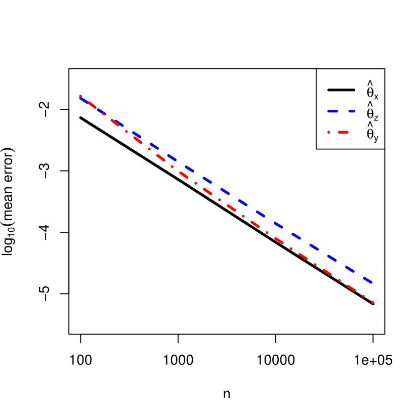
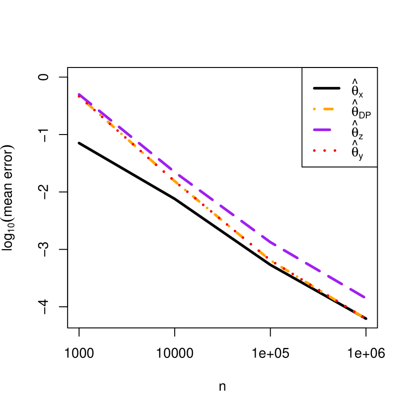
For our simulations, we treat the fitted parameters as the true parameters, to ensure that model assumptions are met. We simulate from the fitted model at sample sizes $n\in\{10^{2},10^{3},10^{4},10^{5}\}$ and compare the performance in terms of the fitted probabilities for each bin of the contingency table. The results are plotted in Figure 1(a), with both axes on log-scale. The “mean error” is the average squared $\ell_{2}$ distance between the estimated parameter vector and the true parameter vector, averaged over 200 replicates. To interpret the plot, note that if the error is of the form $\mathrm{error}=cn^{-1}$, where $c$ is a constant, then $\log(\mathrm{error})=c+(-1)\log(n)$. So, the slope represents the convergence rate, and the vertical offset represents the asymptotic variance. In Figure 1(a), we see that the curve for ${\hat{\theta}_{Y}}$, based on one-step samples, approaches the curve for ${\hat{\theta}_{X}}$, indicating that they have the same asymptotic rate and variance. On the other hand, the curve for ${\hat{\theta}_{Z}}$, based on parametric bootstrap samples, has the same slope, but does not approach the ${\hat{\theta}_{X}}$ curve, indicating that ${\hat{\theta}_{Z}}$ has the same rate but inflated variance. In fact, Theorem 2 indicates that $\operatorname{Var}({\hat{\theta}_{Z}})\approx 2\operatorname{Var}({\hat{\theta}_{X}})$.

We see that our procedure approximately preserves the sufficient statistics, similar to sampling from a conditional distribution. Previous work has proposed procedures to sample directly from conditional distributions for contingency table data. However, these approaches require sophisticated tools from algebraic statistics, and are computationally expensive (e.g., MCMC) (Karwa and Slavković, 2013). In contrast, our approach is incredibly simple to implement and highly computationally efficient. Our approach is also applicable for a wide variety of models, whereas the techniques to sample directly from the conditional distribution often require a tailored approach for each setting.

6.3 Differentially private beta distributed synthetic data

In this example, we assume that $X_{1},\ldots,X_{n}\overset{\text{i.i.d.}}{\sim}\mathrm{Beta}(\alpha,\beta)$, where $\alpha,\beta\geq 1$, and our goal is to produce differentially private (DP) synthetic data. Often, to ensure finite sensitivity, the data are clamped to artificial bounds $[a,b]$, introducing bias in the DP estimate. Typically, these bounds are fixed in $n$, resulting in asymptotically negligible noise, but $O_{p}(1)$ bias. In Section S2 of the Supplementary Materials, we show that it is possible to increase the bounds in $n$ to produce both noise and bias of order $o_{p}(n^{-1/2})$, resulting in an efficient DP estimator. In this section, we show through simulations that using this estimator along with Algorithm 1 results in a DP sample with optimal asymptotics.

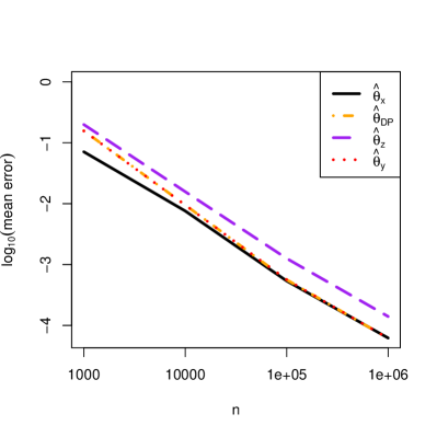
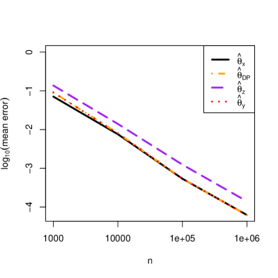
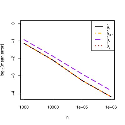
For the simulation, we sample $X_{1},\ldots,X_{n}\overset{\text{i.i.d.}}{\sim}\mathrm{Beta}(5,3)$, with varying sample sizes, $n\in\{10^{3},10^{4},10^{5},10^{6}\}$. We estimate ${\hat{\theta}_{X}}$ with the MLE. Using $\epsilon=1$, we clamp and add Laplace noise to the sufficient statistics to obtain our privatized summary statistics (see Section S2 of the Supplementary Materials for details), and then obtain $\hat{\theta}_{DP}$ by maximizing the log-likelihood with the privatized values plugged in for the sufficient statistics. We sample $Z_{1},\ldots,Z_{n}\overset{\text{i.i.d.}}{\sim}f_{\hat{\theta}_{DP}}$ and calculate the MLE ${\hat{\theta}_{Z}}$. We draw $(Y_{i})_{i=1}^{n}$ from Algorithm 1 using $\hat{\theta}_{DP}$ in place of ${\hat{\theta}_{X}}$. In Figure S.3, we plot the mean squared $\ell_{2}$ error between each estimate of $\theta$ from the true value $(5,3)$, over 200 replicates. From the log-scale plot, we see that $\hat{\theta}_{DP}$ and ${\hat{\theta}_{Y}}$ have the same asymptotic performance as the MLE, whereas ${\hat{\theta}_{Z}}$ has inflated variance. See Example 6.2 for more explanation of this interpretation. Section S.4.1 of the Supplementary Materials contains additional simulations where the value of $\epsilon$ is varied.

6.4 DP two sample proportion test

(a) Under the null hypothesis, the empirical cumulative distribution of both tests. $\theta_{X}=\theta_{Y}=.3$. Results based on 10,000 replicates.

(b) Empirical power at type I error $.05$. $\theta_{X}=.3$, $\theta_{Y}$ is varied along the $x$-axis. Results averaged from 10,000 replicates for each value of $\theta_{Y}$.

Figure 2: Simulations for the DP two sample proportion test of Section 6.4. In red is the one-step test, and in blue is the parametric bootstrap test. Sample sizes are $n=m=200$, privacy parameter is $\epsilon=1$, and type I error is $.05$.

In this section, we illustrate how the one-step samples can be used to perform approximate hypothesis tests. We base the simulation on a problem in differential privacy, where we are given only access to DP summary statistics and are tasked with testing a hypothesis on the generating distribution for the (missing) private data. Such settings result in complex distributions which can be difficult to work with directly, making MCMC methods such as in Barber and Janson (2022) cumbersome and potentially intractable. We show through a simulation that the one-step samples give highly accurate $p$-values and improved power compared to the parametric bootstrap.

Suppose we have two independent samples of binary data, one from a “control population” and another from a “treatment population.” We denote $X_{1},\ldots,X_{n}\overset{\text{i.i.d.}}{\sim}\mathrm{Bern}(\theta_{X})$ as the control sample, and $Y_{1},\ldots,Y_{m}\overset{\text{i.i.d.}}{\sim}\mathrm{Bern}(\theta_{Y})$ as the treatment sample. Note that $m$ used in this example is not related to the dimension of $\Omega$, as stated in (R0).

It was shown in Awan and Slavković (2018) and Awan and Slavković (2020) that the Tulap distribution is the optimal DP mechanism to generate uniformly most powerful hypothesis tests and uniformly most accurate confidence intervals for Bernoulli data. Thus, to satisfy $\epsilon$-differential privacy, the data curators release the following noisy statistics: $\widetilde{X}=\sum_{i=1}^{n}X_{i}+N_{1}$ and $\widetilde{Y}=\sum_{i=1}^{m}Y_{i}+N_{2}$, where $N_{1},N_{2}\overset{\text{i.i.d.}}{\sim}\mathrm{Tulap}\{0,\exp(-\epsilon),0\}$ and the sample sizes $m$ and $n$ are released without modification. Recall that in the $\mathrm{Tulap}(m,b,q)$ distribution, $m\in\mathbb{R}$ is a location parameter, $b\in(0,\infty)$ is related to the scale/shape with higher values increasing the dispersion, and $q$ is a truncation parameter with $0$ indicating that no truncation takes place. In our case, $N_{i}\overset{d}{=}G_{1}-G_{2}+U$, where $G_{1},G_{2}\overset{\text{i.i.d.}}{\sim}\mathrm{Geom}\{1-\exp(-\epsilon)\}$ and $U\sim\mathrm{Unif}(-1/2,1/2)$. We can think of $\widetilde{X}$ and $\widetilde{Y}$ as noisy counts for the control and treatment groups, respectively.

Based only on the privatized summary statistics $\widetilde{X}$ and $\widetilde{Y}$, we are to test $H_{0}:\theta_{X}=\theta_{Y}$ versus $H_{1}:\theta_{X}{<}\theta_{Y}$. Without privacy, there exists a uniformly most powerful test, which is constructed by conditioning on the total number of ones: $\sum_{i=1}^{n}X_{i}+\sum_{j=1}^{m}Y_{j}$, a complete sufficient statistic under the null hypothesis. However, with the noisy counts, it can be verified that there is not a low-dimensional sufficient statistic. On the other hand, an efficient estimator for $\theta_{X}=\theta_{Y}$ under the null hypothesis is $\hat{\theta}(\widetilde{X},\widetilde{Y})=\min[\max\{(\widetilde{X}+\widetilde{Y})/(m+n),0\},1]$. Note that deriving the exact distribution of $(\widetilde{X},\widetilde{Y})\mid\hat{\theta}(\widetilde{X},\widetilde{Y})$ is fairly complex, involving the convolution of distributions. However, the one-step method can easily produce approximate samples from this conditional distribution. In what follows, we use the one-step algorithm, given in Algorithm 1 and investigate the properties of a hypothesis test based on this conditional distribution in comparison with a parametric bootstrap test.

Recall that without privacy, the uniformly most powerful test uses the test statistic $Y$, and threshold computed from the conditional distribution of $Y|X+Y$ under the null hypothesis. With privacy, we use the test statistic $\widetilde{Y}$, the noisy count of ones in the treatment group, and compute the $p$-values based on $\widetilde{Y}\mid\hat{\theta}(\widetilde{X},\widetilde{Y})$. In particular, we compare the performance of this test versus the parametric bootstrap test, which uses the test statistic $\widetilde{Y}$ based on the approximate sampling distribution, which is the convolution of $\mathrm{Binom}\{m,\hat{\theta}(\widetilde{X},\widetilde{Y})\}$ and $\mathrm{Tulap}\{0,\exp(-\epsilon),0\}$.

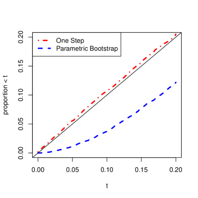
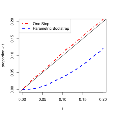
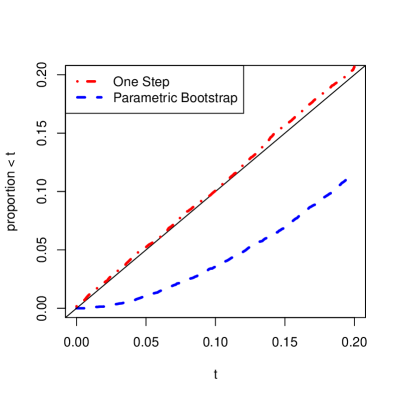
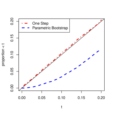
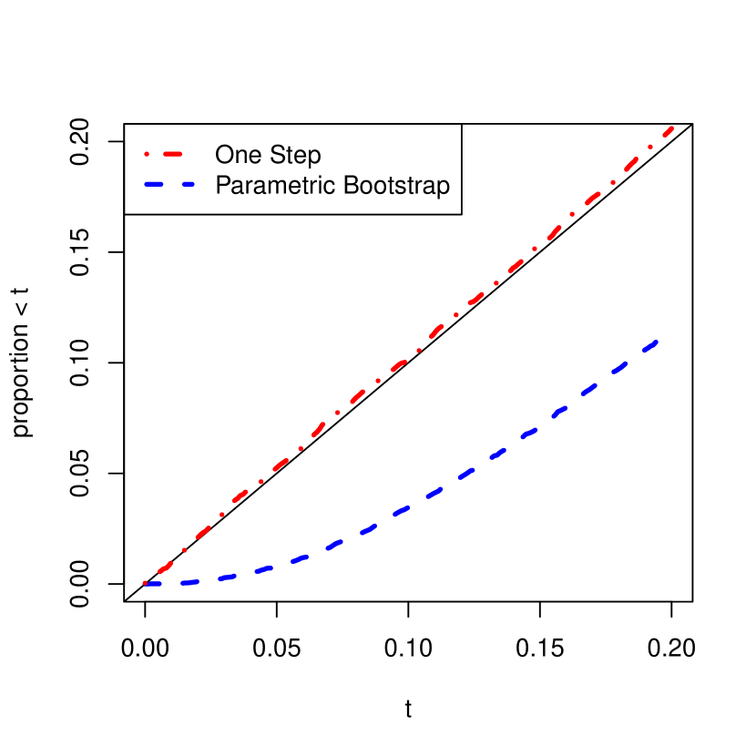
For the simulation, we use the sample size $n=m=200$, fix $\theta_{X}=0.3$, set the privacy parameter to $\epsilon=1$, and base the simulation on 10,000 replicates. Under the null hypothesis, where $\theta_{Y}=\theta_{X}$, we plot the empirical cumulative distribution function (CDF) for the $p$-values of the proposed test as well as for the parametric bootstrap test in Figure 2(a). Recall that a properly calibrated $p$-value will have the CDF of $U(0,1)$. We see that the empirical CDF of the $p$-values for the one-step test closely approximate the ideal CDF, whereas the $p$-values of the parametric bootstrap test are overly conservative.

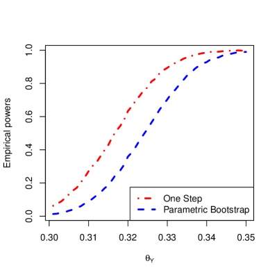
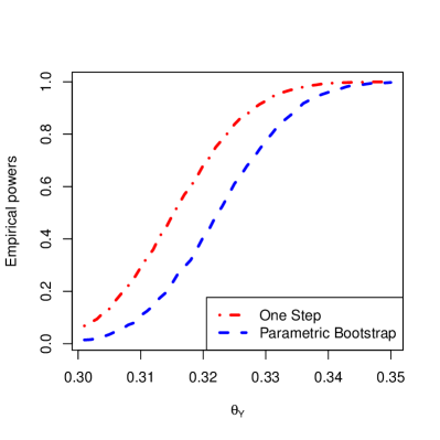
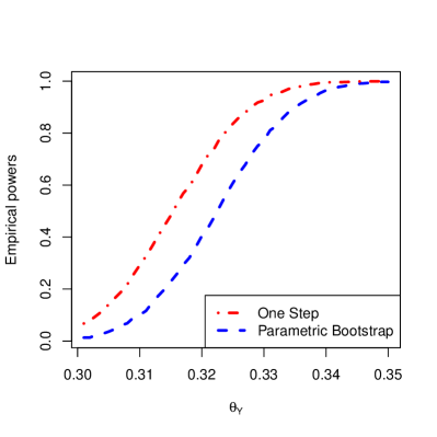
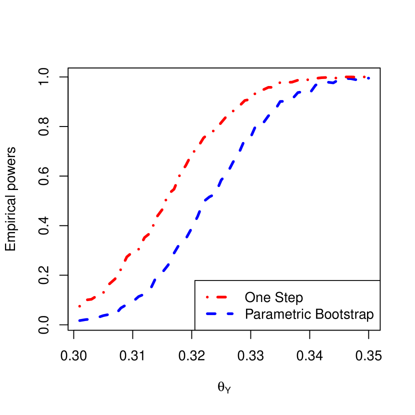
Next, we study the power of the one-step test versus the parametric bootstrap test in Figure 2(b). For this simulation, we set $n=m=200$, fix $\theta_{X}=.3$, and set $\epsilon=1$. We vary the value of $\theta_{Y}$ along the $x$-axis by increments of $.001$ and plot the empirical power of the two tests, averaged over 10,000 replicates for each value of $\theta_{Y}$. We see that the one-step test offers a considerable increase in power over the bootstrap test. Section S.4.2 of the Supplementary Materials contains additional simulations where the value of $\epsilon$ is varied.

7 Discussion

We proposed a simple method of producing synthetic data from a parametric model, which approximately preserves efficient statistics. We also provided evidence in Section 5 that the one-step synthetic data results in a distribution which approaches the true underlying distribution. Both of these properties are in contrast to the common approach of sampling from a fitted model, which we showed results in inefficient estimators and inconsistent synthetic data. Our one-step approach is also widely applicable to parametric models and is both easily implemented and highly computationally efficient. Our approach also allows for both partially synthetic data, as well as differentially private fully synthetic data by incorporating a DP efficient estimator.

Besides synthetic data, there is also promise for using the one-step approach for hypothesis tests as well. Barber and Janson (2022) showed that one can produce powerful and accurate hypothesis tests by conditioning on an efficient statistic for the null model. However, their approach is likelihood based and requires MCMC methods for implementation. In problems with high-dimensional latent variables such an approach is inapplicable, for example in differential privacy where the entire private database is latent. The one-step approach offers a computationally efficient alternative, which we demonstrated in Section 6.4 gives a more accurate and powerful test that the parametric bootstrap.

In Section 5, we studied the distributional properties of a modified version of the one-step method, which suggested that the one-step synthetic data converges to the true joint distribution as the sample size increases. We also saw in Section 6.1 that in the case of the Burr distribution, the Kolmogorov-Smirnov test cannot distinguish between our synthetic sample and the true distribution which generated the original sample, supporting the conjecture that the one-step sample is consistent. In future work, we propose to formally prove that the total variation distance between the one-step samples (rather than an approximation) and the true sampling distribution goes to zero as the sample sizes goes to infinity. This will provide additional theoretical justification for using the one-step method for synthetic data and hypothesis tests. Future researchers may investigate whether the data-augmentation MCMC algorithm of Ju et al. (2022) could enable the approach of Barber and Janson (2022) to be applied to DP problems.

While our approach was focused on parametric models, similar to Theorem 2, there is a loss of “efficiency” when sampling from a non-parametric model as well. Similar to the approach in this paper, it may be advantageous to sample from a non-parametric model conditional on the sample having “similar” estimates as the original data. An interesting future direction would be to formalize and investigate this direction.

Appendix S1 Background on differential privacy

In this section, we review the basics of differential privacy (DP), which was proposed by Dwork et al. (2006) as a framework to develop methods of preserving privacy, with mathematical guarantees. Intuitively, the constraint of differential privacy requires that for all possible databases, the change in one person’s data does not significantly change the distribution of outputs. Consequently, having observed the DP output, an adversary cannot accurately determine the input value of any single person in the database. Definition 12 gives a formal definition of DP. In Definition 12, $h:\mathcal{X}^{n}\times\mathcal{X}^{n}\rightarrow\mathbb{Z}^{\geq 0}$ represents the Hamming metric, defined by $h(\underline{x},\underline{x}^{\prime})=\#\{i\mid x_{i}\neq x^{\prime}_{i}\}$.

Definition 12 (Differential privacy: Dwork et al. (2006)).

Let the privacy parameter $\epsilon>0$ and the sample size $n\in\{1,2,\ldots\}$ be given. Let $\mathcal{X}$ be any set, and $(\mathcal{Y},\mathcal{S})$ a measurable space. Let $\mathcal{M}=\{M_{\underline{x}}\mid\underline{x}\in\mathcal{X}^{n}\}$ be a set of probability measures on $(\mathcal{Y},\mathcal{S})$, which we call a mechanism. We say that $\mathcal{M}$ satisfies $\epsilon$-differential privacy ($\epsilon$-DP) if $M_{\underline{x}}(S)\leq e^{\epsilon}M_{\underline{x}^{\prime}}(S)$ for all $S\in\mathcal{S}$ and all $\underline{x},\underline{x}^{\prime}\in\mathcal{X}^{n}$ such that $h(\underline{x},\underline{x}^{\prime})=1$.

An important property of differential privacy is that it is invariant to post-processing. Applying any data-independent procedure to the output of a DP mechanism preserves $\epsilon$-DP (Dwork et al., 2014, Proposition 2.1). Furthermore, Smith (2011) demonstrated that under conditions similar to (R1)-(R3), there exist efficient DP estimators for parametric models. Using these techniques, the one-step procedure can produce DP synthetic data by using a DP efficient statistic.

Remark 13.

Besides Definition 12, there are many other variations of differential privacy, the majority of which are relaxations of Definition 12 which also allow for efficient estimators. For instance, approximate DP (Dwork et al., 2006), concentrated DP (Dwork and Rothblum, 2016; Bun and Steinke, 2016), truncated-concentrated DP (Bun et al., 2018), and Renyi DP (Mironov, 2017) all allow for efficient estimators. On the other hand, local differential privacy (Kasiviswanathan et al., 2011; Duchi et al., 2013) in general does not permit efficient estimators and would not fit in our framework. For an axiomatic treatment of formal privacy, see Kifer and Lin (2012).

One of the earliest and simplest privacy mechanisms is the Laplace mechanism. Given a statistic $T$, the Laplace mechanism adds independent Laplace noise to each entry of the statistic, with scale parameter proportional to the sensitivity of the statistic. Informally, the sensitivity of $T$ is the largest amount that $T$ changes, when one person’s data is changed in the dataset.

Proposition 14 (Sensitivity and Laplace: Dwork et al. (2006)).

Let the privacy parameter $\epsilon>0$ be given, and let $T:\mathcal{X}^{n}\rightarrow\mathbb{R}^{p}$ be a statistic. The $\ell_{1}$-sensitivity of $T$ is $\Delta_{n}(T)=\sup\lVert T(\underline{x})-T(\underline{x}^{\prime})\rVert_{1},$ where the supremum is over all $\underline{x},\underline{x}^{\prime}\in\mathcal{X}^{n}$ such that $h(\underline{x},\underline{x}^{\prime})=1$. Provided that $\Delta_{n}(T)$ is finite, releasing the vector $\left\{T_{j}(\underline{x})+L_{j}\right\}_{j=1}^{p}$ satisfies $\epsilon$-DP, where $L_{1},\ldots,L_{p}\overset{\text{i.i.d.}}{\sim}\mathrm{Laplace}\left\{\Delta_{n}(T)/\epsilon\right\}$.

Appendix S2 Deriving an DP efficient estimator for the beta distribution

We assume that $X_{1},\ldots,X_{n}\overset{\text{i.i.d.}}{\sim}\mathrm{Beta}(\alpha,\beta)$, where $\alpha,\beta\geq 1$, and our goal is to produce differentially private (DP) synthetic data. Recall that $X_{i}$ takes values in $[0,1]$ and has pdf $f_{X}(x)=x^{\alpha-1}(1-x)^{\beta-1}/B(\alpha,\beta)$, where $B$ is the Beta function.

Often, to ensure finite sensitivity, the data are clamped to artificial bounds $[a,b]$, introducing bias in the DP estimate. Typically, these bounds are fixed in $n$, resulting in asymptotically negligible noise, but $O_{p}(1)$ bias. However, we show that it is possible to increase the bounds in $n$ to produce both noise and bias of order $o_{p}(n^{-1/2})$, resulting in an efficient DP estimator. We show through simulations that using this estimator along with Algorithm 1 results in a DP sample with optimal asymptotics. While we work with the beta distribution, this approach may be of value for other exponential family distributions as well. We note that the asymptotics of clamping bounds have appeared in other DP works, but which are not immediately applicable to our setting (e.g., Smith, 2011; Kamath et al., 2020).

Recall that $n^{-1}\sum_{i=1}^{n}\log(X_{i})$ and $n^{-1}\sum_{i=1}^{n}\log(1-X_{i})$ are sufficient statistics for the beta distribution. We will add Laplace noise to each of these statistics to achieve differential privacy. However, the sensitivity of these quantities is unbounded. First we pre-process the data by setting $\widetilde{X}_{i}=\min\{\max(X_{i},t),1-t\},$ where $t$ is a threshold that depends on $n$. Then the $\ell_{1}$-sensitivity of the pair of sufficient statistics is $\Delta(t)=2n^{-1}\left|\log(t)-\log(1-t)\right|$. We add independent noise to each of the statistics from the distribution $\mathrm{Laplace}\{\Delta(t)/\epsilon\}$, which results in $\epsilon$-DP versions of these statistics. Finally, we estimate $\theta=(\alpha,\beta)$ by plugging in the privatized sufficient statistics into the log-likelihood function and maximizing over $\theta$. The resulting parameter estimate satisfies $\epsilon$-DP by post-processing.

We must carefully choose the threshold $t$ to ensure that the resulting estimate is efficient. The choice of $t$ must satisfy $\Delta(t)=o(n^{-1/2})$ to ensure that the noise does not affect the asymptotics of the likelihood function. We also require that both $P(X_{i}<t)=o(n^{-1/2})$, and $P(X_{i}>1-t)=o(n^{-1/2})$ to ensure that $\widetilde{X}_{i}=X_{i}+o_{p}(n^{-1/2})$, which limits the bias to $o_{p}(n^{-1/2})$. For the beta distribution, we can calculate that $P(X_{i}<t)=O(t^{\alpha})$ and $P(X_{i}>1-t)=O(t^{\beta})$. Since we assume that $\alpha,\beta\geq 1$, so long as $t=o(n^{-1/2})$ the probability bounds will hold. Taking $t=\min[1/2,10/\{\log(n)\sqrt{n}\}]$ satisfies $t=o(n^{-1/2})$, and we estimate the sensitivity as

$$\Delta(t)\leq 2n^{-1}\log(t^{-1})\leq 2n^{-1}\log\{\log(n)\sqrt{n}\}=O\{\log(n)/n\}=o(n^{-1/2}),$$

which satisfies our requirement for $\Delta$. While there are other choices of $t$ which would satisfy the requirements, our threshold was chosen to optimize the finite sample performance, so that the asymptotics could be illustrated with smaller sample sizes.

Appendix S3 Proofs and technical lemmas

For two distributions $P$ and $Q$ on $\mathbb{R}^{k}$, the Kolmogorov-Smirnov distance (KS-distance) is $\mathrm{KS}(P,Q)=\sup_{R\text{ rectangle}}|P(R)-Q(R)|$, where the supremum is over all axis-aligned rectangles. If $F_{P}$ and $F_{Q}$ are the multivariate cdfs of $P$ and $Q$, then $\lVert F_{P}-F_{Q}\rVert_{\infty}\leq\mathrm{KS}(P,Q)\leq 2^{k}\lVert F_{P}-F_{Q}\rVert_{\infty}$, so convergence in distribution is equivalent to convergence in KS-distance (Smith, 2011). By definition, we have that $\mathrm{TV}(P,Q)\geq\mathrm{KS}(P,Q)$.

Proof of Theorem 2.

First we will establish the asymptotic distribution of ${\hat{\theta}_{Z}}$. Recall that by efficiency, we know that $\sqrt{n}\{{\hat{\theta}_{X}}-\theta\}\overset{d}{\rightarrow}N\{0,I^{-1}(\theta)\}$ and $\sqrt{n}[{\hat{\theta}_{Z}}-E\{{\hat{\theta}_{Z}}\mid{\hat{\theta}_{X}}\}]\mid{\hat{\theta}_{X}}\overset{d}{\rightarrow}N[0,I^{-1}\{{\hat{\theta}_{X}}\}]$. Then by Slutsky’s theorem, we have that $\sqrt{n}[{\hat{\theta}_{Z}}-E\{{\hat{\theta}_{Z}}\mid{\hat{\theta}_{X}}\}]\overset{d}{\rightarrow}N\{0,I^{-1}(\theta)\}$. We can easily compute that $\operatorname{Cov}[{\hat{\theta}_{Z}}-E\{{\hat{\theta}_{Z}}\mid{\hat{\theta}_{X}}\},{\hat{\theta}_{X}}]=0$ using the law of total covariance. So, we have that $\sqrt{n}[{\hat{\theta}_{Z}}-E\{{\hat{\theta}_{Z}}\mid{\hat{\theta}_{X}}\}+{\hat{\theta}_{X}}-\theta]\overset{d}{\rightarrow}N\{0,2I^{-1}(\theta)\}$. We also know that $\sqrt{n}[E\{{\hat{\theta}_{Z}}\mid{\hat{\theta}_{X}}\}-{\hat{\theta}_{X}}]=o_{p}(1)$, since $E\{{\hat{\theta}_{Z}}\mid{\hat{\theta}_{X}}\}={\hat{\theta}_{X}}+o_{p}(n^{-1/2})$. Together, we have that $\sqrt{n}\{{\hat{\theta}_{Z}}-\theta\}\overset{d}{\rightarrow}N\{0,2I^{-1}(\theta)\}$.

$$\mathrm{TV}\left(\underline{X},\underline{Z}\right) \geq\mathrm{TV}\left\{\sqrt{n}({\hat{\theta}_{X}}-\theta),\sqrt{n}({\hat{\theta}_{X}}-\theta)\right\}$$ (S3.1)

$$\geq\mathrm{KS}\left\{\sqrt{n}({\hat{\theta}_{X}}-\theta),\sqrt{n}({\hat{\theta}_{X}}-\theta)\right\}$$ (S3.2)

$$\geq\mathrm{KS}\left[N\{0,I^{-1}(\theta)\},N\{0,2I^{-1}(\theta)\}\right]-\mathrm{KS}\left[\sqrt{n}({\hat{\theta}_{X}}-\theta),N\{0,I^{-1}(\theta)\}\right]$$ (S3.3)

$$\phantom{=}-\mathrm{KS}\left[\sqrt{n}({\hat{\theta}_{Z}}-\theta),N\{0,2I^{-1}(\theta)\}\right]$$ (S3.4)

$$=\mathrm{KS}\left[N\{0,I^{-1}(\theta)\},N\{0,2I^{-1}(\theta)\}\right]+o(1)$$ (S3.5)

$$\geq\Phi\left\{-\frac{\sqrt{\log(4)}}{\sqrt{2}}\right\}-\Phi\left\{-\sqrt{\log(4)}\right\}+o(1)$$ (S3.6)

$$\geq.083+o(1)$$ (S3.7)

where (S3.1) is by the data processing inequality, (S3.2) uses the KS-distance as a lower bound on total variation, (S3.4) applies two triangle inequalities since KS-distance is a metric, and (S3.5) uses the asymptotic distributions of ${\hat{\theta}_{X}}$ and ${\hat{\theta}_{Z}}$.

To establish S3.6, consider the following. Denote $\sigma^{2}=(I^{-1}(\theta))_{1,1}$. Then consider the sequence of rectangles $R_{i}=\{x\in\mathbb{R}^{k}\mid-(i+1)\sigma\leq x_{1}\leq-\sqrt{\log(4)}\sigma,\text{ and }-i\leq x_{j}\leq i,\forall j\neq 1\}$. Note that $R_{i}\subset R_{i+1}$ and $\bigcup_{i=1}^{\infty}R_{i}=\{x\in\mathbb{R}\mid x_{1}\leq-\sqrt{\log(4)}\sigma\}$. Denote by $P$ the probability measure for $N\{0,I^{-1}(\theta)\}$ and $Q$ the probability measure for $N\{0,I^{-1}(\theta)\}$. Then

$$\mathrm{KS}\left[N\{0,I^{-1}(\theta)\},N\{0,2I^{-1}(\theta)\}\right] \geq\lim_{i\rightarrow\infty}|P(R_{i})-Q(R_{i})|$$

$$=\left|\lim_{i\rightarrow\infty}P(R_{i})-\lim_{i\rightarrow\infty}Q(R_{i})\right|$$

$$=\left|P\left(\bigcup_{i=1}^{\infty}R_{i}\right)-Q\left(\bigcup_{i=1}^{\infty}R_{i}\right)\right|$$

$$=\Phi\left\{-\frac{\sqrt{\log(4)}}{\sqrt{2}}\right\}-\Phi\left\{-\sqrt{\log(4)}\right\}$$

$$\geq.083.$$

∎

For the following proofs, we will overload the $\frac{d}{d\theta}$ operator when working with multivariate derivatives. For a function $f:\mathbb{R}^{p}\rightarrow\mathbb{R}$, we write $\frac{d}{d\theta}f(\theta)$ to denote the $p\times 1$ vector of partial derivatives $(\frac{\partial}{\partial\theta_{j}}f(\theta))_{j=1}^{p}$. For a function $g:\mathbb{R}^{p}\rightarrow\mathbb{R}^{q}$, we write $\frac{d}{d\theta}g(\theta)$ to denote the $p\times q$ matrix $(\frac{\partial}{\partial\theta_{j}}g_{k}(\theta))_{j,k=1}^{p,q}$.

Lemmas 15 and 16 are used for the proof of Theorem 4. Parts 1 and 2 of Lemma 15 can be rephrased as the following: $\hat{\theta}$ is efficient if and only if it is consistent and $n^{-1}\sum_{i=1}^{n}S(\hat{\theta},X_{i})=o_{p}(n^{-1/2})$. The third property of Lemma 15 is similar to many standard expansions used in asymptotics, for example in Van der Vaart (2000). However, we require the expansion for arbitrary efficient estimators, and include a proof for completeness.

Lemma 15.

Suppose $X_{1},\ldots,X_{n}\overset{\text{i.i.d.}}{\sim}f_{\theta_{0}}$, and assume that (R1)-(R3) hold. Let $\hat{\theta}_{X}$ be an efficient estimator, which is a sequence of zeros of the score function. Suppose that $\widetilde{\theta}_{X}$ is a $\sqrt{n}$-consistent estimator of $\theta_{0}$. Then

1. If $n^{-1}\sum_{i=1}^{n}S(\widetilde{\theta}_{X},X_{i})=o_{p}(n^{-1/2})$, then $\widetilde{\theta}_{X}-\hat{\theta}_{X}=o_{p}(n^{-1/2})$.

2. If $\widetilde{\theta}_{X}$ is efficient, then $n^{-1}\sum_{i=1}^{n}S(\widetilde{\theta}_{X},X_{i})=o_{p}(n^{-1/2})$.

3. If $\widetilde{\theta}_{X}$ is efficient, then $\widetilde{\theta}_{X}=\theta_{0}+I^{-1}(\theta_{0})n^{-1}\sum_{i=1}^{n}S(\theta_{0},X_{i})+o_{p}(n^{-1/2})$.

Proof.

As $\widetilde{\theta}_{X}$ and $\hat{\theta}_{X}$ are both $\sqrt{n}$-consistent, we know that $\widetilde{\theta}_{X}-\hat{\theta}_{X}=O_{p}(n^{-1/2})$. So, we may consider a Taylor expansion of the score function about $\widetilde{\theta}_{X}=\hat{\theta}_{X}$.

$$\begin{split}n^{-1}\sum_{i=1}^{n}S(\widetilde{\theta}_{X},X_{i})&=n^{-1}\sum_{i=1}^{n}S(\hat{\theta}_{X},X_{i})+\left\{\frac{d}{d\theta}n^{-1}\sum_{i=1}^{n}S(\theta,X_{i})\Big{|}_{\theta={\hat{\theta}_{X}}}\right\}(\widetilde{\theta}_{X}-\hat{\theta}_{X})+O_{p}(n^{-1})\\ &=0+\left\{\frac{d}{d\theta}n^{-1}\sum_{i=1}^{n}S(\theta,X_{i})\big{|}_{\theta={\hat{\theta}_{X}}}+O_{p}(n^{-1/2})\right\}(\widetilde{\theta}_{X}-\hat{\theta}_{X})\\ &=\left\{-I(\theta_{0})+o_{p}(1)\right\}(\widetilde{\theta}_{X}-\hat{\theta}_{X}),\end{split}$$ (S3.8)

where we used assumptions (R1)-(R3) to justify that 1) the second derivative is bounded in a neighborhood about $\theta_{0}$ (as both $\hat{\theta}_{X}$ and $\widetilde{\theta}_{X}$ converge to $\theta_{0}$), 2) the derivative of the score converges to $-I(\theta_{0})$ by Lehmann (2004, Theorem 7.2.1) along with the Law of Large Numbers, and 3) that $I(\theta_{0})$ is finite, by (R3).

To establish property 1, note that the left hand side of Equation (S3.8) is $o_{p}(n^{-1/2})$ implying that $\left(\widetilde{\theta}_{X}-\hat{\theta}_{X}\right)=o_{p}(n^{-1/2})$. For property 2, recall that by Lehmann (2004, Page 479), if $\widetilde{\theta}_{X}$ and $\hat{\theta}_{X}$ are both efficient, then $\left(\widetilde{\theta}_{X}-\hat{\theta}_{X}\right)=o_{p}(n^{-1/2})$. Plugging this into the right hand side of Equation (S3.8) gives $n^{-1}\sum_{i=1}^{n}S(\widetilde{\theta}_{X},X_{i})=o_{p}(n^{-1/2})$, establishing property 2.

For property 3, we consider a slightly different expansion:

$$o_{p}(n^{-1/2}) =n^{-1}\sum_{i=1}^{n}S(\widetilde{\theta},X_{i})$$

$$=n^{-1}\sum_{i=1}^{n}S(\theta_{0},X_{i})+\frac{d}{d\theta_{0}}n^{-1}\sum_{i=1}^{n}S(\theta_{0},X_{i})(\widetilde{\theta}-\theta_{0})+O_{p}(n^{-1}),$$

$$=n^{-1}\sum_{i=1}^{n}S(\theta_{0},X_{i})+\{-I(\theta_{0})+o_{p}(1)\}(\widetilde{\theta}-\theta_{0})+O_{p}(n^{-1})$$

where we used property 2 for the first equality, expanded the score about $\hat{\theta}_{X}=\theta_{0}$ for the second, and justify the $O_{p}(n^{-1})$ by (R2). By (R1)-(R2) and Law of Large Numbers along with Lehmann (2004, Theorem 7.2.1), we have the convergence of the derivative of score to $-I(\theta_{0})$. By (R3), $I(\theta_{0})$ is invertible. Solving the equation for $\widetilde{\theta}_{X}$ gives the desired result. ∎

Lemma 16.

Assume that (R0)-(R4) hold, and let $\omega_{1},\ldots,\omega_{n}\overset{\text{i.i.d.}}{\sim}P$. Then

$$n^{-1}\sum_{i=1}^{n}\frac{d}{d\theta}S\{\theta,X_{\theta}(\omega_{i})\}=o_{p}(1).$$

Proof.

First we can express the derivative as

$$n^{-1}\sum_{i=1}^{n}\frac{d}{d\theta}S\{\theta,X_{\theta}(\omega_{i})\}=n^{-1}\sum_{i=1}^{n}\left[\frac{d}{d\alpha}S\{\alpha,X_{\theta}(\omega_{i})\}+\frac{d}{d\alpha}S\{\theta,X_{\alpha}(\omega_{i})\}\right]\Big{|}_{\alpha=\theta}.$$

The result follows from the Law of Large Numbers, provided that

$$E_{\omega\sim P}\left[\frac{d}{d\alpha}S\{\alpha,X_{\theta}(\omega)\}+\frac{d}{d\alpha}S\{\theta,X_{\alpha}(\omega)\}\right]\Big{|}_{\alpha=\theta}=0.$$

The expectation of the first term is $-I(\theta)$, by Lehmann (2004, Theorem 7.2.1). For the second term, we compute

$$E_{\omega\sim P}\frac{d}{d\alpha}S\{\theta,X_{\alpha}(\omega)\}\Big{|}_{\alpha=\theta} =\int_{\Omega}\frac{d}{d\alpha}S\{\theta,X_{\alpha}(\omega)\}\Big{|}_{\alpha=\theta}\pi(\omega)\ d\omega$$ (S3.9)

$$=\frac{d}{d\alpha}\int_{\Omega}S\{\theta,X_{\alpha}(\omega)\}\ \pi(\omega)\ d\omega\Big{|}_{\alpha=\theta}$$ (S3.10)

$$=\frac{d}{d\alpha}\int_{\mathbb{R}^{d}}S(\theta,x)f_{\alpha}(x)\ dx\Big{|}_{\alpha=\theta}$$ (S3.11)

$$=\int_{\mathbb{R}^{d}}\frac{d}{d\alpha}S(\theta,x)f_{\alpha}(x)\Big{|}_{\alpha=\theta}\ dx$$ (S3.12)

$$=\int_{\mathbb{R}^{d}}S(\theta,x)\left\{\frac{d}{d\alpha}f_{\alpha}(x)\Big{|}_{\alpha=\theta}\right\}^{\top}\ dx$$ (S3.13)

$$=\int_{\mathbb{R}^{d}}S(\theta,x)\left\{\frac{\frac{d}{d\theta}f_{\theta}(x)}{f_{\theta}(x)}\right\}^{\top}f_{\theta}(x)\ dx$$ (S3.14)

$$=\int_{\mathbb{R}^{d}}S(\theta,x)S^{\top}(\theta,x)f_{\theta}(x)\ dx$$ (S3.15)

$$=E_{X\sim\theta}\left\{S(\theta,X)S^{\top}(\theta,X)\right\}$$ (S3.16)

$$=I(\theta),$$ (S3.17)

where for (S3.10) we use the bounded-ness of $\Omega$ from (R0) and (R4) to interchange the derivative and integral; for (S3.11), we apply a change of variables, using the fact that $f_{\alpha}(\omega)$ is the density for the random variable $X_{\alpha}(\omega)$; and for (S3.12), we use (R2) and the dominate convergence theorem to change the order of the derivative and integral again. ∎

Proof of Theorem 6.

We expand ${\hat{\theta}_{Z}}$ about ${\hat{\theta}_{X}}$ using part 3 of Lemma 15:

$${\hat{\theta}_{Z}}={\hat{\theta}_{X}}+I^{-1}\{{\hat{\theta}_{X}}\}n^{-1}\sum_{i=1}^{n}S\{{\hat{\theta}_{X}},X_{{\hat{\theta}_{X}}}(\omega_{i})\}+o_{p}(n^{-1/2})$$ (S3.18)

The score can be expanded about ${\hat{\theta}_{X}}=\theta_{0}$:

$$n^{-1}\sum_{i=1}^{n}S\{{\hat{\theta}_{X}},X_{{\hat{\theta}_{X}}}(\omega_{i})\}$$

$$=n^{-1}\sum_{i=1}^{n}S\{\theta_{0},X_{\theta_{0}}(\omega_{i})\}+\left[\frac{d}{d\widetilde{\theta}}n^{-1}\sum_{i=1}^{n}S\{\widetilde{\theta},X_{\widetilde{\theta}}(\omega_{i})\}\right]\{{\hat{\theta}_{X}}-\theta_{0}\}$$

$$=n^{-1}\sum_{i=1}^{n}S\{\theta_{0},X_{\theta_{0}}(\omega_{i})\}+o_{p}(1)O_{p}(n^{-1/2}),$$

where $\widetilde{\theta}$ is between ${\hat{\theta}_{X}}$ and $\theta_{0}$; by Lemma 16, we justify that the derivative is $o_{p}(1)$.

Combining this derivation along with the fact that $I^{-1}\{{\hat{\theta}_{X}}\}=I^{-1}(\theta_{0})+o_{p}(1)$ by the continuous mapping theorem, we have the following equation:

$${\hat{\theta}_{Z}}={\hat{\theta}_{X}}+I^{-1}(\theta_{0})n^{-1}\sum_{i=1}^{n}S\{\theta_{0},X_{\theta_{0}}(\omega_{i})\}+o_{p}(n^{-1/2}).$$ (S3.19)

Using the same techniques, we do an expansion for ${\hat{\theta}_{Y}}$ about $\theta^{*}=2{\hat{\theta}_{X}}-{\hat{\theta}_{Z}}$:

$${\hat{\theta}_{Y}} =\theta^{*}+I^{-1}(\theta^{*})n^{-1}\sum_{i=1}^{n}S\{\theta^{*},X_{\theta^{*}}(\omega_{i})\}+o_{p}(n^{-1/2})$$ (S3.20)

$$=\theta^{*}+I^{-1}(\theta_{0})n^{-1}\sum_{i=1}^{n}S\{\theta_{0},X_{\theta_{0}}(\omega_{i})\}+o_{p}(n^{-1/2})$$ (S3.21)

$$=\theta^{*}+\{{\hat{\theta}_{Z}}-{\hat{\theta}_{X}}\}+o_{p}(n^{-1/2})$$ (S3.22)

$$={\hat{\theta}_{X}}+o_{p}(n^{-1/2}),$$ (S3.23)

where line (S3.21) is a similar expansion as used for equation (S3.18), in line (S3.22) we substituted the expression from (S3.19), and line (S3.23) uses the fact that as $n\rightarrow\infty$, $\theta^{*}=2{\hat{\theta}_{X}}-{\hat{\theta}_{Z}}$ with probability tending to one. Indeed, since $2{\hat{\theta}_{X}}-{\hat{\theta}_{Z}}$ is a consistent estimator of $\theta_{0}$, we have that as $n\rightarrow\infty$, $P\{2{\hat{\theta}_{X}}-{\hat{\theta}_{Z}}\in\Theta\}\geq P\{2{\hat{\theta}_{X}}-{\hat{\theta}_{Z}}\in B(\theta_{0})\}\rightarrow 1$. ∎

Proof of Lemma 10.

For a fixed $\theta\in\Theta$, for $\omega\sim P$, the random variable $Y=X_{\theta}(\omega)$ is distributed with probability measure $PX_{\theta}^{-1}$: for any measurable set $E$, $P(Y\in E)=PX_{\theta}^{-1}(E)$. We denote by $P^{n}_{\Omega}$ the joint probability measure on $\Omega^{n}$, and $(PX_{\theta}^{-1})^{n}$ the joint probability measure on $\mathbb{R}^{d\times n}$.

Given $\theta^{*}\in\Theta$, our goal is to derive the probability distribution of the random variables $X_{\theta^{*}}(\omega_{1}),\ldots,$ $X_{\theta^{*}}(\omega_{n})$ conditioned on the event that $\{\omega_{1},\ldots,\omega_{n}\mid\hat{\theta}\{X_{\theta^{*}}(\omega_{i})\}=\hat{\vartheta}\}$. However, this event may have zero probability. Instead, we will condition on $S_{\hat{\vartheta},\theta^{*}}^{\delta}=\{\omega_{1},\ldots,\omega_{n}\mid\hat{\vartheta}\{X_{\theta^{*}}(\omega)\}\in B_{\delta}(\hat{\vartheta})\}$, where $B_{\delta}(\hat{\vartheta})=\{\theta\mid\lVert\hat{\vartheta}-\theta\rVert\leq\delta\}$, which has positive probability. At the end, we will take the limit as $\delta\rightarrow 0$ to derive the desired distribution.

Let $E\subset\mathbb{R}^{d\times n}$be a measurable set. Then

$$P\{X_{\theta^{*}}(\omega_{1}),\ldots,X_{\theta^{*}}(\omega_{n})\in E\mid\omega_{1},\ldots,\omega_{n}\in S_{\theta^{*},\hat{\vartheta}}^{\delta}\}$$

$$=P(\omega_{1},\ldots,\omega_{n}\in X^{-1}_{\theta^{*}}E\mid\omega_{1},\ldots,\omega_{n}\in S^{\delta}_{\theta^{*},\hat{\vartheta}})$$

$$=\frac{P^{n}(X^{-1}_{\theta^{*}}E\cap S_{\theta^{*},\hat{\vartheta}}^{\delta})}{P^{n}(S_{\theta^{*},\hat{\vartheta}}^{\delta})}$$

$$=\frac{(PX_{\theta^{*}}^{-1})^{n}(E\cap X_{\theta^{*}}S^{\delta}_{\theta^{*},\hat{\vartheta}})}{(PX_{\theta^{*}}^{-1})^{n}(X_{\theta^{*}}S_{\theta^{*},\hat{\vartheta}}^{\delta})},$$

where we used the definition of conditional probability and the fact that $X_{\theta^{*}}^{-1}X_{\theta^{*}}S_{\theta^{*},\hat{\vartheta}}^{\delta}=S_{\theta^{*},\hat{\vartheta}}^{\delta}$.

This last expression shows that $X_{\theta^{*}}(\omega_{1}),\ldots,X_{\theta^{*}}(\omega_{n})$ conditioned on $\underline{\omega}\in S_{\theta^{*},\hat{\vartheta}}^{\delta}$ is distributed as $f^{n}_{\theta^{*}}\{y_{1},\ldots,y_{n}\mid\hat{\theta}(\underline{y})\in B_{\delta}(\hat{\vartheta})\}$. This derivation is valid for all $\delta>0$. Taking the limit as $\delta\rightarrow 0$ gives the desired formula:

$$Y^{\theta^{*}}_{1},\ldots,Y^{\theta^{*}}_{n}\Big{|}\hat{\theta}(\underline{Y}^{\theta^{*}})=\hat{\theta}(\underline{X})\sim f_{\theta^{*}}^{n}\{y_{1},\ldots,y_{n}\mid\hat{\theta}(\underline{y})=\hat{\theta}(\underline{X})\}.$$

∎

Proof of Theorem 11.

While the distributions $g$ depend on $n$, we will suppress this dependence for notational simplicity. We can then express the desired KL divergence as follows:

First, by the data processing inequality, we can add in the random variable $\hat{\theta}(\underline{X})=\hat{\theta}(\underline{Y})$ to get an upper bound on the KL divergence. We then have closed formulas for the joint distributions $\{X_{1},\ldots,X_{n},\hat{\theta}(\underline{X})\}$ and $\{Y_{1},\ldots,Y_{n},\hat{\theta}(\underline{X})\}$.

$$\mathrm{KL} \left\{X_{1},\ldots,X_{n}\middle|\middle|Y_{1},\ldots,Y_{n}\right\}$$ (S3.24)

$$\leq\mathrm{KL}\left\{X_{1},\ldots,X_{n},\hat{\theta}(\underline{X})\middle|\middle|Y_{1},\ldots,Y_{n},\hat{\theta}(\underline{X})\right\}$$ (S3.25)

$$=\mathrm{KL}\left[f_{\theta}^{n}\{\underline{x}\mid\hat{\theta}(\underline{x})\}g_{\theta}\{\hat{\theta}(x)\}\middle|\middle|f_{\theta_{n}}^{n}\{\underline{x}\mid\hat{\theta}(\underline{x})\}g_{\theta}\{\hat{\theta}(\underline{x})\}\right]$$ (S3.26)

$$=E_{\hat{\vartheta}\sim g(\cdot\mid\underline{X})}E_{\underline{X}\sim f_{\theta}}\log\left\{\frac{f_{\theta}(\underline{X}\mid\hat{\vartheta})g_{\theta}(\hat{\vartheta})}{f_{\theta_{n}}(\underline{X}\mid\hat{\vartheta})g_{\theta}(\hat{\vartheta})}\right\}$$ (S3.27)

$$=E_{\hat{\vartheta}\sim g(\cdot\mid\underline{X})}E_{\underline{X}\sim f_{\theta}}\log\left\{\frac{f_{\theta}(\underline{X})g(\hat{\vartheta}\mid\underline{X})}{f_{\theta_{n}}(\underline{X}\mid\hat{\vartheta})g_{\theta}(\hat{\vartheta})}\right\}$$ (S3.28)

$$=E_{\hat{\vartheta}\sim g(\cdot\mid\underline{X})}E_{\underline{X}\sim f_{\theta}}\log\left[\frac{f_{\theta}(\underline{X})g(\hat{\vartheta}\mid\underline{X})}{\{f_{\theta_{n}}(\underline{X})g(\hat{\vartheta}\mid\underline{X})/g_{\theta_{n}}(\hat{\vartheta})\}g_{\theta}(\hat{\vartheta})}\right]$$ (S3.29)

$$=E_{\hat{\vartheta}\sim g(\cdot\mid\underline{X})}E_{\underline{X}\sim f_{\theta}}\log\left\{\frac{f_{\theta}(\underline{X}){g(\hat{\vartheta}\mid\underline{X})}}{f_{\theta_{n}}(\underline{X}){g(\hat{\vartheta}\mid\underline{X})}}\right\}+E_{\hat{\vartheta}\sim g(\cdot\mid\underline{X})}E_{\underline{X}\sim f_{\theta}}\log\left\{\frac{g_{\theta_{n}}(\hat{\vartheta})}{g_{\theta}(\hat{\vartheta})}\right\}$$ (S3.30)

$$=-E_{\underline{X}\sim f_{\theta}}\log\left(\frac{f_{\theta_{n}}(\underline{X})}{f_{\theta}(\underline{X})}\right)+E_{\hat{\vartheta}\sim g_{\theta}}\log\left(\frac{g_{\theta_{n}}(\hat{\vartheta})}{g_{\theta}(\hat{\vartheta})}\right),$$ (S3.31)

Above, line (S3.27) simply applies the definition of KL divergence, and line (S3.29) uses the definition of conditional distribution.

At this point, we need to compute the two expectations of line (S3.31), and show that everything cancels except for an $o_{p}(1)$ term.

We write $\ell(\theta\mid\underline{x})=\sum_{i=1}^{n}\log f_{\theta}(x_{i})$. Using our assumptions, we can expand $\ell(\theta_{n}\mid\underline{x})$:

$$\ell(\theta_{n}\mid\underline{x}) =\ell(\theta\mid\underline{x})+(\theta_{n}-\theta)^{\top}\nabla\ell(\theta\mid\underline{x})+\frac{1}{2}(\theta_{n}-\theta)^{\top}\nabla^{2}\ell(\theta\mid\underline{x})(\theta_{n}-\theta)$$

$$\phantom{=}+\frac{1}{6}\xi^{*}\sum_{i,j,k}(\theta_{n}-\theta)_{i}(\theta_{n}-\theta)_{j}(\theta_{n}-\theta)_{k}\sum_{s=1}^{n}g_{ijk}(x_{s}),$$

where $|\xi^{*}|<1$ and $g_{ijk}(x)$ is an upper bound for $\left|\frac{\partial^{3}\ell(\theta\mid\underline{x})}{\partial\theta_{i}\theta_{j}\theta_{k}}\right|$ for a ball $\theta\in N(\theta)$ which exists by (R3). These expansions are based on those from Serfling (1980). Applying $E_{\underline{X}\sim f_{\theta}}$ to this derivation gives

$$\begin{split}E_{\underline{X}\sim f_{\theta}}\log\left\{\frac{f_{\theta_{n}}(\underline{X})}{f_{\theta}(\underline{X})}\right\}&=0-\frac{n}{2}(\theta_{n}-\theta)^{\top}I(\theta)(\theta_{n}-\theta)\\ &\phantom{=}+O(1)\frac{n}{6}\sum_{i,j,k}\{Eg_{i,j,k}(x)\}(\theta_{n}-\theta)_{i}(\theta_{n}-\theta)_{j}(\theta_{n}-\theta)_{k},\\ &=\frac{-n}{2}(\theta_{n}-\theta)^{\top}I(\theta)(\theta_{n}-\theta)+O(n)\lVert\theta_{n}-\theta\rVert^{3}\end{split}$$ (S3.32)

where the first term is zero as the expected value of the score function is zero by (R3), the second term uses Lehmann (2004, Theorem 7.2.1) and (R3). The $O(1)$ factor in the third term is based on the fact that $|\xi^{*}|\leq 1$. Finally, note that $\sum_{i,j,k}\{Eg_{i,j,k}(x)\}(\theta_{n}-\theta)_{i}(\theta_{n}-\theta)_{j}(\theta_{n}-\theta)_{k}\leq p^{3}\sup_{i,j,k}\{Eg_{i,j,k}(x)\}\lVert\theta_{n}-\theta\rVert^{3}_{\infty}=O(1)\lVert\theta_{n}-\theta\rVert^{3}$. Note that all norms are equivalent in $\mathbb{R}^{p}$, so they can be interchanged up to a factor of $O(1)$.

Next, we will derive a similar formula for $\log g_{\theta^{*}}(\hat{\vartheta})$:

$$\begin{split}\log g_{\theta_{n}}(\hat{\vartheta})&=\log g_{\theta}(\hat{\vartheta})+\nabla\log g_{\theta}(\hat{\vartheta})(\theta_{n}-\theta)+\frac{1}{2}(\theta_{n}-\theta)^{\top}\nabla^{2}\log g_{\theta}(\hat{\vartheta})(\theta_{n}-\theta)\\ &\phantom{=}+\frac{n}{6}\xi_{2}^{*}\sum_{i,j,k}(\theta_{n}-\theta)_{i}(\theta_{n}-\theta)_{j}(\theta_{n}-\theta)_{k}G_{i,j,k}(\hat{\vartheta}),\end{split}$$ (S3.33)

where $|\xi_{2}^{*}|\leq 1$. In order to apply the expectation $E_{\hat{\vartheta}\sim\theta}$ to this equation, we will first show $E_{\hat{\vartheta}\sim\theta}\nabla\log g_{\theta}(\hat{\vartheta})=0$ and $E_{\hat{\vartheta}\sim\theta}\nabla^{2}\log g_{\theta}(\hat{\vartheta})=-nI(\theta)+o(n)$.

$$\left\{E_{\hat{\theta}\sim\theta}\nabla\log g_{\theta}(\hat{\vartheta})\right\}_{j} =\int\left\{\frac{\partial}{\partial\theta_{j}}\log g_{\theta}(\hat{\vartheta})\right\}g_{\theta}(\hat{\vartheta})\ d\hat{\vartheta}$$

$$=\int\frac{\partial}{\partial\theta_{j}}g_{\theta}(\hat{\vartheta})\ d\hat{\vartheta}$$

$$=\int\frac{\partial}{\partial\theta_{j}}\int_{x}f_{\theta}(x)g(\hat{\vartheta}\mid x)\ dx\ d\hat{\vartheta}$$

$$=\int_{\hat{\theta}}\int_{x}\frac{\partial}{\partial\theta_{j}}f_{\theta}(x)g(\hat{\vartheta}\mid x)\ dx\ d\hat{\vartheta}$$

$$=\frac{\partial}{\partial\theta_{j}}\int\int f_{\theta}(x)g(\hat{\vartheta}\mid x)\ dx\ d\hat{\vartheta}$$

$$=0,$$

where we use the assumption (R3) that $\left|\frac{\partial}{\partial\theta_{j}}f_{\theta}(x)\right|$ is bounded above by an integrable function, (R5) that $g(\hat{\vartheta}\mid x)$ is bounded, and the dominated convergence theorem to interchange the derivative and the integral.

Next we work on the second derivative:

$$\left\{E_{\hat{\vartheta}\sim\theta}\nabla^{2}\log g_{\theta}(\hat{\vartheta})\right\}_{j,k} =\int\left\{\frac{\partial^{2}}{\partial\theta_{j}\partial\theta_{k}}\log g_{\theta}(\hat{\vartheta})\right\}g_{\theta}(\hat{\vartheta})\ d\hat{\vartheta}$$

$$=\int\frac{g_{\theta}(\hat{\vartheta})\frac{\partial^{2}}{\partial\theta_{j}\partial\theta_{k}}g_{\theta}(\hat{\vartheta})-\frac{\partial}{\partial\theta_{j}}g_{\theta}(\hat{\vartheta})\left\{\frac{\partial}{\partial\theta_{k}}g_{\theta}(\hat{\vartheta})\right\}^{\top}}{g_{\theta}^{2}(\hat{\vartheta})}g_{\theta}(\hat{\vartheta})\ d\hat{\vartheta}$$

$$=0-E_{\hat{\vartheta}\sim\theta}\left\{\nabla\log g_{\theta}(\hat{\vartheta})\nabla^{\top}\log g_{\theta}(\hat{\vartheta})\right\}_{j,k},$$

where we used (R3) along with the dominated convergence theorem to set the first term equal to zero. We see that $E\nabla^{2}\log g_{\theta}(\hat{\vartheta})=-I_{{\hat{\theta}_{X}}}(\theta)$, where $I_{{\hat{\theta}_{X}}}$ represents the Fisher information of the random variable $\hat{\theta}(\underline{X})\sim g$. It is our current goal to show that $I_{{\hat{\theta}_{X}}}(\theta)=nI(\theta)+o(n)$, where $I(\theta)$ is the Fisher information for one sample $X\sim f_{\theta}$. First note that by the data processing inequality (Zamir, 1998), $I_{\hat{\theta}(\underline{X})}(\theta)\leq I_{X_{1},\ldots,X_{n}}(\theta)=nI(\theta)$, where the inequality represents the positive-definite ordering of matrices. Next, we need to find a matching lower bound. By the Cramér Rao lower bound, we have that

$$\{I_{\hat{\theta}(\underline{X})}(\theta)\}^{-1}\leq\operatorname{Var}\{\hat{\theta}(\underline{X})\}+o(1/n),$$

where $\operatorname{Var}\{{\hat{\theta}_{X}}\}$ is the covariance matrix of the random variable ${\hat{\theta}_{X}}$, and we used the fact that ${\hat{\theta}_{X}}$ is asymptotically unbiased. By the efficiency of $\hat{\theta}(\underline{X})$, we have that

$$\operatorname{Var}\{\hat{\theta}(\underline{X})\}=n^{-1}I^{-1}(\theta)+o(1/n).$$

We then have

$$I_{\hat{\theta}(\underline{X})}(\theta) \geq\left\{n^{-1}I^{-1}(\theta)+o(1/n)\right\}^{-1}=n\{I^{-1}(\theta)+o(1)\}^{-1}=n\{I(\theta)+o(1)\},$$

where for the last equality, we use the following matrix identity:

$$(A+B)^{-1}=A^{-1}-A^{-1}B(A+B)^{-1},$$

where we set $A=I^{-1}(\theta)$ and $B=o(1)$.

Combining our results, we have that

$$E_{\hat{\vartheta}\sim\theta}\nabla^{2}\log g_{\theta}(\hat{\vartheta})=-I_{\hat{\theta}(\underline{X})}(\theta)=n\{-I(\theta)+o(1)\}.$$

Finally, applying the expectation to equation (S3.33), we have

$$\begin{split}E_{\hat{\vartheta}\sim\theta}\log\left\{\frac{g_{\theta_{n}}(\hat{\vartheta})}{g_{\theta}(\hat{\vartheta})}\right\}&=0-\frac{n}{2}(\theta_{n}-\theta)\{I(\theta)+o(1)\}(\theta_{n}-\theta)\\ &\phantom{=}+O(1)\frac{n}{6}\sum_{i,j,k}\{EG_{i,j,k}(\hat{\vartheta})\}(\theta_{n}-\theta)_{i}(\theta_{n}-\theta)_{j}(\theta_{n}-\theta)_{k}\\ &=\frac{-n}{2}(\theta_{n}-\theta)^{\top}I(\theta)(\theta_{n}-\theta)+o(n)\lVert\theta_{n}-\theta\rVert^{2}+O(n)\lVert\theta_{n}-\theta\rVert^{3}.\end{split}$$ (S3.34)

Combining equations (S3.32) and (S3.34), we have

$$\mathrm{KL} \left(X_{1},\ldots,X_{n}\middle|\middle|Y_{1},\ldots,Y_{n}\right)$$

$$\leq\mathrm{KL}\left[f_{\theta}^{n}\{\underline{x}\mid\hat{\theta}(\underline{x})\}g_{\theta}\{\hat{\theta}(x)\}\middle|\middle|f_{\theta_{n}}^{n}\{\underline{x}\mid\hat{\theta}(\underline{x})\}g_{\theta}\{\hat{\theta}(\underline{x})\}\right]$$

$$=-E_{\underline{X}\sim f_{\theta}}\log\left\{\frac{f_{\theta_{n}}(\underline{X})}{f_{\theta}(\underline{X})}\right\}+E_{\hat{\vartheta}\sim g_{\theta}(\hat{\vartheta})}\log\left\{\frac{g_{\theta_{n}}(\hat{\vartheta})}{g_{\theta}(\hat{\vartheta})}\right\}$$

$$=o(n)\lVert\theta_{n}-\theta\rVert^{2}+O(n)\lVert\theta_{n}-\theta\rVert^{3}.$$

∎

Appendix S4 Additional Simulation Results

Figure S.3: Additional simulations for Section 6.3. In normal reading order, $\epsilon=.5,2,4,\infty$. Note that Figure 1(b) in the main paper is for $\epsilon=1$

S4.1 Differentially private beta synthetic data

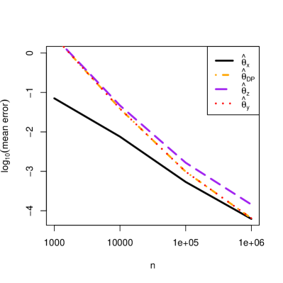
In this section, we consider additional values of $\epsilon$ that are used in the Section 6.3 experiment on differentially private beta distributed synthetic data. All other simulation parameters are identical. We varied $\epsilon=.5,2,4,\infty$ (note that $\epsilon=1$ appears in Figure 1(b) in the main paper). In Figure S.3, we see that at all values of $\epsilon$, ${\hat{\theta}_{Y}}$ is very close to $\hat{\theta}_{DP}$. However, with smaller $\epsilon$ it requires a larger sample size before the performance of ${\hat{\theta}_{Y}}\approx\hat{\theta}_{DP}$ is similar to the MLE ${\hat{\theta}_{X}}$. Note that even with $\epsilon=\infty$, the performance of ${\hat{\theta}_{Z}}$ does not approach that of ${\hat{\theta}_{X}}$.

S4.2 DP two sample proportion test

In this section, we repeat the experiment of Section 6.4 with varying values of $\epsilon$. All other simulation parameters are the same. We varied $\epsilon=.5,2,4,10$ (note that $\epsilon=1$ appears in Figure 1(b) in the main paper). In Figure S.4, we plot the $p$-values of both the one-step and parametric bootstrap tests. We see that the parametric bootstrap $p$-values are very conservative for all values of $\epsilon$, whereas the one-step $p$-values are fairly well-calibrated, although sometimes slightly inflated. In Figure S.5 we plot the power of the two tests for the different $\epsilon$ values. We see that the relative performance of one-step compared to parametric bootstrap is unchanged as we vary $\epsilon$.

Figure S.4: Additional simulations for Section 6.4. In normal reading order, $\epsilon=.5,2,4,10$. Note that Figure 2(a) in the main paper is for $\epsilon=1$

Figure S.5: Additional simulations for Section 6.4. In normal reading order, $\epsilon=.5,2,4,10$. Note that Figure 2(b) in the main paper is for $\epsilon=1$

References

- Agresti (2003) Agresti, A. (2003). Categorical data analysis, Volume 482. John Wiley & Sons.
- Awan and Slavković (2018) Awan, J. and A. Slavković (2018). Differentially private uniformly most powerful tests for binomial data. In Advances in Neural Information Processing Systems, pp. 4208–4218.
- Awan and Slavković (2020) Awan, J. and A. Slavković (2020). Differentially private inference for binomial data. Journal of Privacy and Confidentiality 10(1).
- Barber and Janson (2022) Barber, R. F. and L. Janson (2022). Testing goodness-of-fit and conditional independence with approximate co-sufficient sampling. The Annals of Statistics 50(5), 2514–2544.
- Bun et al. (2018) Bun, M., C. Dwork, G. N. Rothblum, and T. Steinke (2018). Composable and versatile privacy via truncated cdp. In Proceedings of the 50th Annual ACM SIGACT Symposium on Theory of Computing, pp. 74–86.
- Bun and Steinke (2016) Bun, M. and T. Steinke (2016). Concentrated differential privacy: Simplifications, extensions, and lower bounds. In Theory of Cryptography Conference, pp. 635–658. Springer.
- Burridge (2003) Burridge, J. (2003). Information preserving statistical obfuscation. Statistics and Computing 13(4), 321–327.
- Caiola and Reiter (2010) Caiola, G. and J. P. Reiter (2010). Random forests for generating partially synthetic, categorical data. Transactions on Data Privacy 3(1), 27–42.
- Charest (2011) Charest, A.-S. (2011). How can we analyze differentially-private synthetic datasets? Journal of Privacy and Confidentiality 2(2).
- Chen et al. (2006) Chen, Y., I. H. Dinwoodie, and S. Sullivant (2006). Sequential importance sampling for multiway tables. The Annals of Statistics 34(1), 523–545.
- Drechsler (2011) Drechsler, J. (2011). Synthetic datasets for statistical disclosure control: theory and implementation, Volume 201. Springer Science & Business Media.
- Drechsler and Reiter (2008) Drechsler, J. and J. P. Reiter (2008). Accounting for intruder uncertainty due to sampling when estimating identification disclosure risks in partially synthetic data. In International Conference on Privacy in Statistical Databases, pp. 227–238. Springer.
- Drechsler and Reiter (2011) Drechsler, J. and J. P. Reiter (2011). An empirical evaluation of easily implemented, nonparametric methods for generating synthetic datasets. Computational Statistics & Data Analysis 55(12), 3232–3243.
- Duchi et al. (2013) Duchi, J. C., M. I. Jordan, and M. J. Wainwright (2013). Local privacy and statistical minimax rates. In 2013 IEEE 54th Annual Symposium on Foundations of Computer Science, pp. 429–438. IEEE.
- Dwork et al. (2006) Dwork, C., K. Kenthapadi, F. McSherry, I. Mironov, and M. Naor (2006). Our data, ourselves: Privacy via distributed noise generation. In Annual International Conference on the Theory and Applications of Cryptographic Techniques, pp. 486–503. Springer.
- Dwork et al. (2006) Dwork, C., F. McSherry, K. Nissim, and A. Smith (2006). Calibrating noise to sensitivity in private data analysis. In Theory of Cryptography Conference, pp. 265–284. Springer.
- Dwork et al. (2014) Dwork, C., A. Roth, et al. (2014). The algorithmic foundations of differential privacy. Foundations and Trends® in Theoretical Computer Science 9(3–4), 211–407.
- Dwork and Rothblum (2016) Dwork, C. and G. N. Rothblum (2016). Concentrated differential privacy. arXiv preprint arXiv:1603.01887.
- Engen and Lillegård (1997) Engen, S. and M. Lillegård (1997). Stochastic simulations conditioned on sufficient statistics. Biometrika 84(1), 235–240.
- Ferrando et al. (2022) Ferrando, C., S. Wang, and D. Sheldon (2022). Parametric bootstrap for differentially private confidence intervals. In International Conference on Artificial Intelligence and Statistics, pp. 1598–1618. PMLR.
- Guerrier et al. (2019) Guerrier, S., E. Dupuis-Lozeron, Y. Ma, and M.-P. Victoria-Feser (2019). Simulation-based bias correction methods for complex models. Journal of the American Statistical Association 114(525), 146–157.
- Hall et al. (2013) Hall, R., A. Rinaldo, and L. Wasserman (2013). Differential privacy for functions and functional data. Journal of Machine Learning Research 14(Feb), 703–727.
- Harder et al. (2021) Harder, F., K. Adamczewski, and M. Park (2021). Dp-merf: Differentially private mean embeddings with randomfeatures for practical privacy-preserving data generation. In International conference on artificial intelligence and statistics, pp. 1819–1827. PMLR.
- Hardt et al. (2012) Hardt, M., K. Ligett, and F. McSherry (2012). A simple and practical algorithm for differentially private data release. In Advances in Neural Information Processing Systems, pp. 2339–2347.
- Hundepool et al. (2012) Hundepool, A., J. Domingo-Ferrer, L. Franconi, S. Giessing, E. S. Nordholt, K. Spicer, and P.-P. De Wolf (2012). Statistical disclosure control. John Wiley & Sons.
- Jiang et al. (2021) Jiang, B., A. E. Raftery, R. J. Steele, and N. Wang (2021). Balancing inferential integrity and disclosure risk via model targeted masking and multiple imputation. Journal of the American Statistical Association 117(537), 52–66.
- Jordon et al. (2018) Jordon, J., J. Yoon, and M. van der Schaar (2018). Pate-gan: Generating synthetic data with differential privacy guarantees. In International Conference on Learning Representations.
- Ju et al. (2022) Ju, N., J. Awan, R. Gong, and V. Rao (2022). Data augmentation mcmc for bayesian inference from privatized data. Advances in Neural Information Processing Systems 35, 12732–12743.
- Kamath et al. (2020) Kamath, G., V. Singhal, and J. Ullman (2020). Private mean estimation of heavy-tailed distributions. In Conference on Learning Theory, pp. 2204–2235. PMLR.
- Karwa and Slavković (2012) Karwa, V. and A. Slavković (2012). Differentially private graphical degree sequences and synthetic graphs. In International Conference on Privacy in Statistical Databases, pp. 273–285. Springer.
- Karwa and Slavković (2013) Karwa, V. and A. Slavković (2013). Conditional inference given partial information in contingency tables using Markov bases. Wiley Interdisciplinary Reviews: Computational Statistics 5(3), 207–218.
- Kasiviswanathan et al. (2011) Kasiviswanathan, S. P., H. K. Lee, K. Nissim, S. Raskhodnikova, and A. Smith (2011). What can we learn privately? SIAM Journal on Computing 40(3), 793–826.
- Kifer and Lin (2012) Kifer, D. and B.-R. Lin (2012). An axiomatic view of statistical privacy and utility. Journal of Privacy and Confidentiality 4(1).
- Lane et al. (2014) Lane, J., V. Stodden, S. Bender, and H. Nissenbaum (2014). Privacy, big data, and the public good: Frameworks for engagement. Cambridge University Press.
- Le Cam et al. (1956) Le Cam, L. et al. (1956). On the asymptotic theory of estimation and testing hypotheses. In Proceedings of the Third Berkeley Symposium on Mathematical Statistics and Probability, Volume 1: Contributions to the Theory of Statistics. The Regents of the University of California.
- Lehmann (2004) Lehmann, E. L. (2004). Elements of large-sample theory. Springer Science & Business Media.
- Li et al. (2018) Li, B., V. Karwa, A. Slavković, and R. C. Steorts (2018). A privacy preserving algorithm to release sparse high-dimensional histograms. Journal of Privacy and Confidentiality 8(1).
- Liew et al. (1985) Liew, C. K., U. J. Choi, and C. J. Liew (1985). A data distortion by probability distribution. ACM Transactions on Database Systems (TODS) 10(3), 395–411.
- Lillegard and Engen (1999) Lillegard, M. and S. Engen (1999). Exact confidence intervals generated by conditional parametric bootstrapping. Journal of Applied Statistics 26(4), 447–459.
- Lindqvist and Taraldsen (2005) Lindqvist, B. H. and G. Taraldsen (2005). Monte carlo conditioning on a sufficient statistic. Biometrika 92(2), 451–464.
- Lindqvist and Taraldsen (2007) Lindqvist, B. H. and G. Taraldsen (2007). Conditional monte carlo based on sufficient statistics with applications. In Advances In Statistical Modeling And Inference: Essays in Honor of Kjell A Doksum, pp. 545–561. World Scientific.
- Lindqvist and Taraldsen (2013) Lindqvist, B. H. and G. Taraldsen (2013). Exact statistical inference for some parametric nonhomogeneous poisson processes. Journal of The Iranian Statistical Society 12(1), 113–126.
- Liu (2016) Liu, F. (2016). Model-based differentially private data synthesis. arXiv preprint arXiv:1606.08052.
- Machanavajjhala et al. (2008) Machanavajjhala, A., D. Kifer, J. Abowd, J. Gehrke, and L. Vilhuber (2008). Privacy: Theory meets practice on the map. In 2008 IEEE 24th International Conference on Data Engineering, pp. 277–286. IEEE.
- Mateo-Sanz et al. (2004) Mateo-Sanz, J. M., A. Martínez-Ballesté, and J. Domingo-Ferrer (2004). Fast generation of accurate synthetic microdata. In International Workshop on Privacy in Statistical Databases, pp. 298–306. Springer.
- McClure and Reiter (2012) McClure, D. and J. P. Reiter (2012). Differential privacy and statistical disclosure risk measures: An investigation with binary synthetic data. Transactions on Data Privacy 5(3), 535–552.
- McDonald (2008) McDonald, J. B. (2008). Some generalized functions for the size distribution of income. In Modeling Income Distributions and Lorenz Curves, pp. 37–55. Springer.
- Mironov (2017) Mironov, I. (2017). Rényi differential privacy. In 2017 IEEE 30th Computer Security Foundations Symposium (CSF), pp. 263–275. IEEE.
- Muralidhar and Sarathy (2003) Muralidhar, K. and R. Sarathy (2003). A theoretical basis for perturbation methods. Statistics and Computing 13(4), 329–335.
- Pozrikidis (2014) Pozrikidis, C. (2014). An introduction to grids, graphs, and networks. Oxford University Press.
- Raghunathan et al. (2003) Raghunathan, T. E., J. P. Reiter, and D. B. Rubin (2003). Multiple imputation for statistical disclosure limitation. Journal of Official Statistics 19(1), 1.
- Reiter (2002) Reiter, J. P. (2002). Satisfying disclosure restrictions with synthetic data sets. Journal of Official Statistics 18(4), 531.
- Reiter (2005) Reiter, J. P. (2005). Using cart to generate partially synthetic public use microdata. Journal of Official Statistics 21(3), 441.
- Reiter and Raghunathan (2007) Reiter, J. P. and T. E. Raghunathan (2007). The multiple adaptations of multiple imputation. Journal of the American Statistical Association 102(480), 1462–1471.
- Rubin (1993) Rubin, D. B. (1993). Statistical disclosure limitation. Journal of Official Statistics 9(2), 461–468.
- Serfling (1980) Serfling, R. L. (1980). Approximation Theorems in Mathematical Statistics. New York: Wiley.
- Slavković and Lee (2010) Slavković, A. B. and J. Lee (2010). Synthetic two-way contingency tables that preserve conditional frequencies. Statistical Methodology 7(3), 225–239.
- Smith (2011) Smith, A. (2011). Privacy-preserving statistical estimation with optimal convergence rates. In Proceedings of the Forty-Third Annual ACM Symposium on Theory of Computing, pp. 813–822.
- Taraldsen and Lindqvist (2018) Taraldsen, G. and B. H. Lindqvist (2018). Conditional fiducial models. Journal of Statistical Planning and Inference 195, 141–152.
- Ting et al. (2005) Ting, D., S. Fienberg, and M. Trottini (2005). Romm methodology for microdata release. Monographs of Official Statistics, 89.
- Triastcyn and Faltings (2018) Triastcyn, A. and B. Faltings (2018). Generating differentially private datasets using GANs.
- Ullman and Vadhan (2020) Ullman, J. and S. Vadhan (2020). Pcps and the hardness of generating synthetic data. Journal of Cryptology 33(4), 2078–2112.
- Van der Vaart (2000) Van der Vaart, A. W. (2000). Asymptotic statistics. Cambridge University Press.
- Xie et al. (2018) Xie, L., K. Lin, S. Wang, F. Wang, and J. Zhou (2018). Differentially private generative adversarial network. arXiv preprint arXiv:1802.06739.
- Xu et al. (2019) Xu, C., J. Ren, D. Zhang, Y. Zhang, Z. Qin, and K. Ren (2019). Ganobfuscator: Mitigating information leakage under gan via differential privacy. IEEE Transactions on Information Forensics and Security 14(9), 2358–2371.
- Zamir (1998) Zamir, R. (1998). A proof of the fisher information inequality via a data processing argument. IEEE Transactions on Information Theory 44(3), 1246–1250.
- Zhang et al. (2017) Zhang, J., G. Cormode, C. M. Procopiuc, D. Srivastava, and X. Xiao (2017). Privbayes: Private data release via bayesian networks. ACM Transactions on Database Systems (TODS) 42(4), 1–41.