Modeling non-Fickian solute transport due to mass transfer and physical heterogeneity on arbitrary groundwater velocity fields

Abstract

We present a hybrid approach to groundwater transport modeling, “CTRW-on-a-streamline”, that allows continuous-time random walk (CTRW) particle tracking on large-scale, explicitly-delineated heterogeneous groundwater velocity fields. The combination of a non-Fickian transport model (in this case, the CTRW) with general heterogeneous velocity fields represents an advance of the current state of the art, in which non-Fickian transport models or heterogeneous velocity fields are employed, but generally not both. We present a general method for doing this particle tracking that fully separates the model parameters characterizing macroscopic flow, subscale advective heterogeneity, and mobile-immobile mass transfer, such that each can be directly specified a priori from available data. The method is formalized and connections to classic CTRW and subordination approaches are made. Numerical corroboration is presented.

1 Introduction

1.1 Motivation

Classical Eulerian numerical models that employ a discretized advection-dispersion equation (ADE) are often not sufficient to model groundwater solute transport with needed realism because they fail to capture important physical heterogeneity and mass transfer at scales beneath their discretization scale. Additionally, their flow models may be oversmoothed even above their discretization scale due to a lack of constraining information. Non-Fickian transport models are a generalization of the classical transport models that can capture a wider range of physics, and have demonstrated success at capturing realistic chemical physics that cannot be modeled by classic approaches by introducing additional model flexibility. In the case of the popular continuous-time random walk (CTRW) approach, the additional flexibility comes in the free selection of a waiting time probability distribution, $\psi(t)$, that better describes the dispersion process.

However, when capturing the effects of groundwater velocity heterogeneity, there has commonly been an “all or nothing” choice. Either model all the heterogeneity explicitly and then use an ADE-based transport model, or model all heterogeneity implicitly by considering its effects, combined with those of any other sources of non-Fickian behavior, in selection of the non-Fickian model parameters (e.g., $\psi(t)$). A consequence is that it is difficult to incorporate partial knowledge about large-scale flow into non-Fickian solute transport models, and it is generally difficult to predict correct model parameters a priori, as these depend in non-straightforward ways on the interaction of multiple physical and chemical sources of heterogeneity. This limitation may have reduced the penetration of advanced transport models from academic research into hydrogeologic practice. But whatever the underlying reasons, practitioners have typically favored explicitly heterogeneous models incorporating large-scale flow information coupled with ADE-based transport, whereas researchers have often chosen conversely: employing homogeneous, often quasi-1D, flow alongside more exotic non-Fickian transport models. Ideally, a hybrid approach to modeling would be available (a) allowing usage of explicitly-delineated, spatially-heterogeneous groundwater velocity fields, with non-Fickian transport modeling used only to capture small-scale physics, and (b) whose non-Fickian model parameters have a straightforward relationship to the physics of the natural system they model. Developing such a hybrid approach is the goal of this work.

1.2 Sources of heterogeneity beneath flow model support scale

Before it developing a hybrid approach in which small-scale flow heterogeneity and mass transfer are captured with a stochastic transport model, it is naturally important to understand these processes and their impact on transport, and why a stochastic approach is valuable.

Consider an ideal scenario in which the groundwater flow field is known down to the pore scale in the plume region and computational power is unlimited, with the only stochastic process operative being molecular diffusion. In this situation, solute transport could in theory be captured exactly by a deterministic model, and perhaps by a discretized advection-dispersion equation. However, in realistic scenarios only the volume average groundwater velocity over some larger scale may be known with any precision, and the local-scale velocity fluctuations are random in an epistemic sense: unknown except potentially for their statistics. The first effort to deal with this problem was the so-called macrodispersion theory, which attempts encapsulate the effects of all the unknown velocity fluctuations into an additional Fickian dispersive term, justified by the Central Limit Theorem. While this approach is appropriate for large distances from the solute source and smaller heterogeneity (Hansen et al., 2018), frequently we are interested in understanding solute breakthrough in systems for which these restrictions are not appropriate. In such cases, non-Fickian behavior is generally observed and a more general approach such as usage of the continuous time random walk (CTRW)—where the travel time is captured by a travel time pdf—is appropriate.

The groundwater velocity field is determined by solution of the groundwater flow equation on a (generally) heterogeneous hydraulic conductivity ($K$) field, and it is reasonable that its heterogeneity statistics will determine flow heterogeneity. On the assumption of lognormality of the $K$ field, (typically unrealistically) small log-$K$ variance, and multi-Gaussian correlation structure with light-tailed (exponentially decaying or finitely supported) semivariogram, the macrodispersion theory (Rubin, 2003) provides analytical expressions for the solute transport behavior. However, when these assumptions are violated, we must rely on numerical studies linking heterogeneity and breakthrough curve statistics. There are not many of these in the literature, but to our knowledge, those that exist point strongly in two directions. For mild-to-moderate hydraulic conductivity heterogeneity and multi-Gaussian correlation structure, numerical studies have indicated a lognormal distribution for $\psi(t)$, gradually acquiring power law behavior in the tails as heterogeneity increases (Gotovac et al., 2009; Hansen et al., 2018). We stress that sub-Darcy-scale heterogeneity and trapping may still cause power law tailing even under mild or nonexistent $K$-field heterogeneity, as numerous experiments have shown (see discussion in Berkowitz et al. (2006)). For lognormally distributed $K$ and heavy-tailed (i.e., power law) semivariograms, studies have pointed in different directions. Moslehi and de Barros (2017) analyzed breakthrough in conductivity fields with a single, moderate, heterogeneity ($\sigma^{2}_{\ln K}$ = 4) and different strengths of power law semivariogram, finding their breakthrough curves generally well described by lognormal distributions, except for some heavy tailing. Bolster and Dentz (2012) considered mildly heterogeneous, but power law correlated, velocity fields, showing analytically, under the validity conditions of their perturbation expansion, that breakthrough curves show power law tailing with the same exponent as the semivariogram. Zhang et al. (2013) performed a large-scale simulation study on highly heterogeneous realizations generated with depositional simulators (i.e., non-multivariate-Gaussian realizations), finding generally power-law behavior across realizations. They further found that where the islands of the lowest-$K$ material had a power law size distribution (loosely analogous to the correlation length in a semivariogram), that this determined the tail exponent. However, the relationship between exponents that they uncovered differed from that of Bolster and Dentz (2012). Edery et al. (2014) performed a numerical particle tracking study on moderate-to-large heterogeneity ($\sigma^{2}_{\ln K}$ = 3 to 7) multivariate Gaussian fields, finding their breakthrough curves generally well described by a truncated power law distribution; we also speculate, based on analysis for Hansen et al. (2018), that the lower-heterogeneity breakthrough curves would also be well described by lognormal distributions, again deviating towards power law behavior at late time. Finally, Tyukhova et al. (2016) considered an idealized problem of transport in a homogeneous medium with embedded spheres, each homogeneous and each with random (uniform) conductivity. They found that for truncated power law conductivity distribution, breakthrough curves were truncated power law, and that for (truncated) lognormal conductivity distributions, breakthrough curves were lognormal.

In addition to the heterogeneous advection just discussed, a second category of transport process may also cause sub-support-scale heterogeneity: mobile-immobile mass transfer (MIMT), or broadly speaking, trapping processes. This category naturally includes adsorption, in which solute is truly immobilized, but also includes processes in which diffusion roughly orthogonal to the local advection direction moves solute into low-permeability regions in which advection is essentially inoperative. It is known that such physics may be captured by CTRW (Berkowitz et al., 2006, 2016). However, they are also frequently treated by a variety of specialized modeling approaches, including retardation factors, explicit two-domain models (e.g., Neretnieks, 1980), dual porosity approaches (Gerke and van Genuchten, 1993), kinetic sorption models (see, e.g., Fetter, 1999), multi-rate mass transfer (MRMT) (Haggerty and Gorelick, 1995), and fractal-MRMT / memory function approaches (Schumer et al., 2003). We note that heterogeneous advection has also been modeled with MRMT (the so-called MRMT-1 of Dentz and Berkowitz (2003)), but for our purposes we treat it separately.

1.3 Numerical modeling of transport with particle tracking

A common approach to numerical modeling of transport is to write the governing partial differential or integro-differential equation and then solve it analytically or semi-analytically using transform methods. However, this approach is generally only tenable in systems with spatially-uniform parameters. For systems with spatially non-uniform parameters, solution of the governing equation must be accomplished by spatial discretization. This introduces the problems of numerical dispersion and (in reactive models) numerical mixing. Where the governing equation contains a temporal integral, as in non-Fickian transport models, numerical instability becomes a concern, too.

Particle tracking approaches avoid these difficulties, and have been found to work well under very general conditions, as long as enough particles are used. A classic particle tracking algorithm typically uses a constant temporal user-specified step size, $\Delta_{t}$. The simplest possible particle update conditions apply in the case of pure advection (i.e., streamline tracing) iteration of each particle’s position would be performed according to the following equations:

$$\bm{x}_{n+1} = \bm{x}_{n}+\bm{v}(\bm{x}_{n})\Delta_{t}$$ (1)

$$t_{n+1} = t_{n}+\Delta_{t}$$ (2)

To model Fickian dispersion one modifies (1) to read

$$\bm{x}_{n+1}=\bm{x}_{n}+\bm{v}(\bm{x}_{n})\Delta_{t}+\bm{\Delta}_{\bm{x},n}^{D},$$ (3)

where in the case of isotropic diffusion

$$\Delta_{\bm{x},n}^{D}\equiv\bm{\eta},$$ (4)

where $\bm{\eta}$ is a random 3-vector, each of whose components $\eta_{i}\sim N(0,2D\Delta_{t})$, and $D$ is the Fick’s Law constant. For CTRW particle tracking, either (1) or (3) may be used, but the time step selection in (2) is modified so as to be selected at random:

$$\Delta_{t}\sim\psi(\Delta_{t}),$$ (5)

where $\psi$ is a probability distribution function with strictly non-negative support.

Below, we will see how to modify these equations to capture the sources of heterogeneity discussed in Section 1.2 while also incorporating coarse-scale flow information. Our strategy is to perform a CTRW that makes essentially fixed-length steps down the streamlines of the coarse-scale flow field. Such an approach is sometimes referred to as a time-domain random walk (TDRW), a special case of CTRW originally developed in 1D based on ADE transport solutions (Banton et al., 1997; Reimus and James, 2002), and subsequently developed to model MIMT in discrete fractures by Delay and Bodin (2001). This approach was formalized using CTRW transition-time distribution theory by Cvetkovic and Haggerty (2002) and explicit solutions for rock matrix residence times were presented by Painter et al. (2008). Subsequently, the TDRW approach was employed in a large number of particle tracking studies on discrete fracture networks. For transport in heterogeneous porous media, Hansen and Berkowitz (2014) introduced a cognate CTRW approach, capturing transport as a series of transitions among parallel planes orthogonal to mean flow (leading to a quasi-1D upscaled transport model). Subsequently, another quasi-1D approach that approximates flow in heterogeneous media with an effective medium and also incorporates MIMT was discussed by Cvetkovic et al. (2016). TDRW solutions based on classical (ADE) ideas and that include transverse dispersion were also presented by Bodin (2015).

Some other works whose concepts we build upon include Cortis et al. (2004), who introduced a zoned approach to CTRW modeling of subsurface transport, with different CTRW parameters manually defined for different regions. The idea that a travel time distribution for advection with random motion can be expressed as the product of an average velocity and a distribution representing heterogeneity, is latent in the Kreft and Zuber (1978) solution for advective-dispersive breakthrough (see the factorization we present in (20)). This idea has been employed in the context of scaling CTRW transition time distributions to a local advection velocity by Srinivasan et al. (2010) and by Kang et al. (2014). The concept of mapping an advective travel time to a random total time including multiple immobilization events was presented by Benson and Meerschaert (2009) for exponentially-distributed mobile and immobile times. A similar approach has been adopted for arbitrary immobile time distributions by Hansen et al. (2016) and by Russian et al. (2016). Finally, the CTRW-on-a-streamline approach can be seen as extending the ideas of Cirpka and Nowak (2003) to general, potentially non-Fickian, transport: instead of using an additional dispersion term to capture small-scale flow field variability excluded from a smoothed deterministic model, we propose to use a CTRW transition time distribution.

Developing from the ideas in these works, we present a complete treatment capturing local-scale heterogeneous advection, MIMT, and transverse dispersion using fully 3D streamlines and presenting explicit, physics-based formulae for the relevant CTRW transition-time distributions.

2 Development of the CTRW-on-a-streamline approach

2.1 Theory underlying the approach

For pure streamline tracing, it is possible to choose a fixed distance, $d$, that is traversed in equation (1) by adjusting the time step with reference to the local velocity: $\Delta_{t_{O},n}=\frac{d}{\|\textbf{v}(\textbf{x}_{n})\|}$. We add the subscript $n$ on each time step, $\Delta t_{n}$, because the time taken with each advective step is now variable and the variable $t_{O}$ stands for “operational time”, whose significance will be explained below. This fixed distance increment, variable time approach to large-scale advection is advantageous versus the common fixed time increment, variable distance approach because it sets us up to use a CTRW transition time distribution to capture small-scale advective heterogeneity and mass transfer. To wit: we first define a random walk transition to occur whenever another increment $d$ downgradient is traversed. We then seek to define the conditional pdf, $\psi(\Delta_{t_{C}}|\Delta_{t_{O}})$, for the true or clock time, $\Delta_{t_{C}}$, taken to traverse that increment when small-scale physical heterogeneity and mass transfer are considered, conditioned on the notional or operational time that would be taken to traverse the same segment by pure advection on the large-scale streamlines.

Each segment of length $d$ of a large-scale streamline may be conceptualized as representing a flux-weighted ensemble, or “bundle”, of small-scale, adjacent stream tubes of length $d$ with varying local harmonic mean hydraulic conductivity. Each small-scale stream tube has a different advection time, $\Delta_{t_{A}}$, and because the small-scale stream tubes in an ensemble are epistemically interchangeable (we have no knowledge of their exact position or of the particular small-scale tube to which a particle being tracked along a large-scale streamline belongs), it is sensible to define a conditional probability distribution, $\phi(\Delta_{t_{A}}|\Delta_{t_{O}})$.

The nature of $\phi(\Delta_{t_{A}}|\Delta_{t_{O}})$ can be characterized by noting that the small-scale stream tubes in an ensemble share approximately the same gradient: justified by the fact that the global head field is an integral quantity and is smooth relative to the underlying hydraulic conductivity ($K$) field. Because $K$ is everywhere independent of the boundary conditions on head that determine the magnitude of the large-scale effective $\bm{v}$, and the head drop is shared by small-scale stream tubes in an ensemble, it follows that the Darcy velocities in each of the tubes in the ensemble always maintain a same constant of proportionality to $\|\bm{v}\|$, regardless of system boundary conditions. And because $d$ is fixed, the same is true of travel time, $\Delta_{t_{A}}$. Thus a simple scaling law applies: $\phi(\Delta_{t_{A}}|\Delta_{t_{O}})\Delta_{t_{O}}=\phi(\Delta_{t_{A}}/\Delta_{t_{O}}|1)=:f(r)$, where $f$ is some unknown pdf, solely determined by the statistics of small-scale heterogeneity, which contains all relevant information for mapping from operational time to true advection time, and $r=\Delta_{t_{A}}/\Delta_{t_{O}}$. Another way of looking at this is that the average of the ratio $\Delta_{t_{A}}$ to $\Delta_{t_{O}}$ is independent of the actual magnitude of $\Delta_{t_{O}}$ (and hence the magnitude of the groundwater velocity). The distribution $f(r)$ is determined by flow heterogeneity alone.

This informal argument is supported by a number of additional lines of evidence. We note that this is true for all advective-dispersive systems (see equation (21)). The formal analysis of Tyukhova et al. (2016) considers transport in a regularly-spaced grid of equal-sized circular inclusions with random (low) conductivity in a uniform higher-conductivity matrix and shows mathematically that the velocity in any each inclusion varies in proportion with the system average flux. Comolli et al. (2016) show how under pure advection, the pdf for fixed distance travel time can be written in terms of the Lagrangian velocity pdf, and that under ergodic conditions the Eulerian velocity pdf determines the Lagrangian. Because the Eulerian pdf naturally scales linearly with global hydraulic gradient, the ratio of $\Delta_{t_{A}}$ to $\Delta_{t_{O}}$ must be independent of average velocity under ergodic conditions.

Once advective heterogeneity is specified by $f(r)$, any MIMT, whether due to diffusion into secondary porosity or to chemical adsorption, can be captured by defining two additional probability distributions. The first distribution is exponential, with a rate constant, $\lambda$, representing the probability of immobilization of mobile solute per unit time traveled. The second, not necessarily exponential, distribution, $g(t)$, represents the time for the length of a single particle immobilization event. The exponential form of the mobile-time distribution is justified by the assumption of randomly located sites that are dense relative to length scale $d$. We note that the $\lambda$ and $g$ approach captures even multiple types of immobilization sites with different capture and release distributions (i.e. multi-rate mass transfer), as the time until the first event for multiple simultaneous exponentially-distributed processes is itself exponential, and we can create an immobilization-site-prevalence-weighted average of the immobilization time pdf’s for the various site types.

To quantify the travel time increase due to MIMT, we can develop a conditional pdf, $\zeta(\Delta_{t_{C}}|\Delta_{t_{A}})$. We note that the total (clock) time is the advection time, $\Delta_{t_{A}}$ plus the delay due to $n$ independent immobilization events each of whose lengths is drawn from $g(t)$. The probability mass function for $i$ immobilization events, $w(i)$, is Poisson distributed with parameter $\lambda\Delta_{t_{A}}$, leading (Billingsley, 1986, p. 262) to probability mass function

$$w(i)=e^{-\lambda\Delta_{t_{A}}}\frac{(\lambda\Delta_{t_{A}})^{i}}{i!},$$ (6)

Our conditional pdf, $\zeta$, is thus a weighted average of $i$-fold autoconvolutions of $g$:

$$\zeta(\Delta_{t_{C}}|\Delta_{t_{A}})=\sum_{i=0}w(i)\times g^{(i*)}(\Delta_{t_{C}}-\Delta_{t_{A}}).$$ (7)

Where sites are sparse, an exponential distribution whose rate constant represents probability of immobilization of mobile solute per streamline distance traveled may instead be more appropriate (Margolin et al., 2003). On this conception, we must understand $\lambda$ as capture probability per unit distance, and $\zeta$ becomes no longer dependent on $\Delta_{t_{A}}$:

$$w(i)=e^{-\lambda d}\frac{(\lambda d)^{i}}{i!},$$ (8)

and we have

$$\zeta(\Delta_{t_{C}}|\Delta_{t_{O}},d)=\sum_{i=0}w(i)\times g^{(i*)}(\Delta_{t_{C}}-\Delta_{t_{O}}).$$ (9)

we will not discuss this second conception further, but it is important to stress its compatibility with our mathematics.

Although it is most convenient computationally to work with $f$, $g$, and $\lambda$, we can easily relate the above analysis to the CTRW transition distribution, $\psi$, by constructing the conditional distribution

$$\psi(\Delta_{t_{C}}|\Delta_{t_{O}})=\int_{0}^{\Delta_{t_{C}}}\zeta(\Delta_{t_{C}}|\Delta_{t_{A}})\ \phi(\Delta_{t_{A}}|\Delta_{t_{O}})\ d\Delta_{t_{A}}.$$ (10)

This can be converted into a classic (unconditional) CTRW distribution by marginalizing

$$\psi(\Delta_{t_{C}})=\int_{0}^{\Delta_{t_{C}}}\psi(\Delta_{t_{C}}|\Delta_{t_{O}})\ h_{d}(\Delta_{t_{O}}),$$ (11)

where $h_{d}$ is an unknown but determinate pdf for the operational time for all transitions of length $d$ anywhere in the domain. We see here two reasons why it is advantageous to employ the CTRW-on-a-streamline approach when large-scale information is available. First, the move $\psi(\Delta_{t_{C}}|\Delta_{t_{O}})$ to $\psi(\Delta_{t_{C}})$ involves a loss of information: under a classic approach, the same spatially-averaged $\psi(\Delta_{t_{C}})$ is used at all locations, inducing a loss of fidelity. Second, it is actually harder to compute this distribution because it depends on an additional a priori unknown pdf that must be constrained by statistical information.

Finally, we note that our analysis has so far detailed no mechanism for transfer of solute laterally between streamlines. This small-scale transverse dispersion is a Fickian process may be incorporated via the $\bm{\Delta}_{\bm{x},n}^{D}$ term in (3). Unlike the isotropic diffusion case (4), here we are only looking to model dispersion in the plane transverse to the streamline. First, we need to compute two orthonormal vectors which are also orthogonal to $\bm{v}$. To do so, an arbitrary vector a, not collinear with $\textbf{v}(\textbf{x})$, is specified. Then, orthonormal vectors are computed

$$\bm{n}_{1} = \frac{\bm{a}\times\bm{v}(\bm{x})}{\|\bm{a}\times\bm{v}(\bm{x})\|_{2}}$$ (12)

$$\bm{n}_{2} = \frac{\bm{n}_{1}\times\bm{v}(\bm{x})}{\|\bm{n}_{1}\times\bm{v}(\bm{x})\|_{2}}$$ (13)

For compactness, we define the matrix $\bm{N}(\bm{v})\equiv[\bm{n}_{1}\ \bm{n}_{2}]$ (i.e., the matrix whose columns are the streamline-orthogonal unit vectors $\bm{n}_{1}$ and $\bm{n}_{2}$), then we define $\bm{\eta}$ to be a 2-vector, each of whose components, $\eta_{i}\sim\mathcal{N}(0,2\alpha_{t}d)$, where $\alpha_{t}$ represents the transverse dispersivity. Finally, the perturbation between streamlines is computed by matrix-vector multiplication:

$$\bm{\Delta}_{\bm{x},n}^{D}=\bm{N}(\bm{v})\bm{\eta}.$$ (14)

2.2 Formal specification

It is straightforward to distill the above analysis into a set of formal equations that define the particle position and time updating rules for the CTRW-on-a-streamline approach. The top level equations are:

$$\bm{x}_{n+1} = \bm{x}_{n}+\bm{v}(\bm{x}_{n})\Delta_{t_{O},n}+\bm{N}(\bm{v}(\bm{x}_{n}))\bm{\eta},$$ (15)

$$t_{C,n+1} = t_{C,n}+\Delta_{t_{C},n},$$ (16)

where

$$\Delta_{t_{O},n} = \frac{d}{\|\bm{v}(\bm{x}_{n})\|},$$ (17)

$$\eta_{i} \sim \mathcal{N}(0,2\alpha_{t}d),$$ (18)

$$\Delta_{t_{C},n} \sim \psi(\Delta_{t_{C},n}|\Delta_{t_{O},n}).$$ (19)

Placed in this form, it is clear that equations (15-19) represent an evolution of the classic CTRW equations, with the conditioning of $\psi$ on $\Delta_{t_{O},n}$ representing the major novelty (the restriction of transverse dispersion to the plane orthogonal to the streamline is a minor novelty). It is also clear from the examination of equations (15-16) that CTRW-on-a-streamline can be seen as a form of subordination technique (Benson and Meerschaert, 2009; Hansen et al., 2016): particle location is updated according to a notional operational time, whereas particle time is updated in accordance with a true clock time.

3 Numerical implementation

3.1 Pseudocode

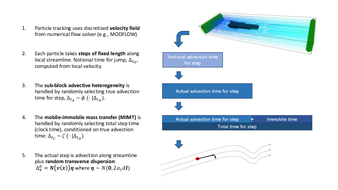
As mentioned, it is not optimal to compute $\Delta_{t_{C},n}$ by parameterizing the distribution $\psi(\Delta_{t_{C},n}|\Delta_{t_{O},n})$ and then drawing random variables from it. Rather, it is easier to build up $\Delta_{t_{C},n}$ by first computing $\Delta_{t_{A},n}$ by drawing from the pdf $f(\cdot)$, defining the advection time per unit operational time, and then computing the additional immobile time by making draws from $\mathrm{Poisson}(\cdot;\lambda\Delta_{t_{A},n})$ and $g(\cdot)$. The following algorithm simulates a particle’s transport in accordance with equations (15-19), by means of these intermediate distributions:

1. For step $n$ = 0, initialize the particle’s position in space and time by constructing the tuple $(\bm{x}_{0},t_{C})$ and decide on streamline tracing increment $d$.

2. Referring to the explicit large-scale discrete velocity field, determine $\bm{v}(\bm{x}_{n})$.

3. Compute the operational time $\Delta_{t_{O},n}$ by using (17).

4. Compute actual advection time $\Delta_{t_{A},n}$ by drawing randomly from the advection-time-per-unit-operational-time pdf $f$, and multiplying that result by $\Delta_{t_{O},n}$.

5. Compute the number of immobilization events, $i$, in advection time $\Delta_{t_{A},n}$ by drawing randomly from the distribution $\mathrm{Poisson}(\cdot;\lambda\Delta_{t_{A},n})$.

6. Draw $i$ random numbers independently from the $g(\cdot)$, the pdf for the length of a single sojourn in the immobile state, and sum them to yield the total time immobile time while traveling $d$ units down the streamline.

7. Compute $\Delta_{t_{C},n}$ by adding total immobile time and $\Delta_{t_{A},n}$.

8. Determine transverse dispersion by computing $\bm{N}(\bm{v}(\bm{x}_{n}))$ with (12-13), drawing the random vector, $\bm{\eta}$, according to (18), and multiplying.

9. Update the particle’s position, $\bm{x}_{n+1}$, according to (15).

10. Update the particle’s clock time, $t_{C,n+1}$, according to (19).

11. Record any events of interest (breakthroughs or particle location snapshots).

12. If $t_{C,n+1}$ is less than the end time for the simulation, increment the step index, $n$, by one and loop back to step 2.

Note that because particles do not interact and have independent clocks, (a) this algorithm can be performed in parallel for multiple particles, and (b) particles can be initialized at different clock times. A schematic diagram summarizing the essential procedural steps is given in Figure 1.

Figure 1: Schematic diagram outlining the essential conceptual steps of the CTRW-on-a-streamline approach.

Of course, to completely specify the algorithm, we need to specify $f(\cdot)$, $\lambda$, and $g(\cdot)$. How this is done depends on the underlying physics to be modeled; considerations are discussed immediately below.

3.2 Specification of advective heterogeneity

Advective heterogeneity refers to varying local pore water velocities experienced by particles as they are advected along a stream tube and experience transverse diffusion. For our purposes, it also incorporates physics that are sometimes considered using MRMT techniques (i.e., the “MRMT-1” class outlined in Dentz and Berkowitz (2003)), namely advection into discrete low-velocity features. The CTRW-on-a-streamline approach captures advective heterogeneity by directly encoding the spectrum of times taken to travel $d$ in the small-scale stream tubes associated with a large-scale streamline in the distribution $\phi(\Delta_{t_{A}}|\Delta_{t_{O}})$, or equivalently in $f(\cdot)$. For predictive modeling purposes, we would like to express the parameters defining the distribution $f(r)$ in terms of well-known parameters describing the subsurface heterogeneity, as in the case of MIMT. For the case of homogeneous local-scale Fickian transport, this is easily accomplished analytically: an inverse Gaussian distribution applies. However, heterogeneity at all scales complicates the picture.

Although, as outlined in the introduction, there is no general theory relating ensemble breakthrough parameters to conductivity field statistics, there are three classes of pdf supported by the literature for capturing advective heterogeneity pdf $f(r)$, each suitable for different problems. These classes are: (i) inverse Gaussian, which derives from Fickian analysis, (ii) lognormal, applicable to mildly or moderately heterogeneous systems, and (iii) power law / truncated power law, perhaps the most widely applicable, capturing the strong heterogeneity often encountered at field scale. We discuss how to specify each for use with the CTRW-on-a-streamline approach in turn.

3.2.1 Fickian dispersion: inverse Gaussian behavior

For longitudinal, local-scale Fickian dispersion, the travel time pdf for a transition of length $d$, is simply the well-known Inverse Gaussian distribution, as calculated by, e.g., Kreft and Zuber (1978). We write it in factored form as

$$\phi(\Delta_{t_{A}})=\frac{1}{\Delta_{t_{A}}}\left[\frac{d}{\sqrt{4\pi\alpha_{l}\|v\|\Delta_{t_{A}}}}\exp\left\{\frac{-(d-\|v\|\Delta_{t_{A}})^{2}}{4\alpha_{l}\|v\|\Delta_{t_{A}}}\right\}\right],$$ (20)

where, $\alpha_{l}$ is the Fickian longitudinal dispersivity. Note that the quantity in square brackets is dimensionless. Further noting that $r=\Delta_{t_{A}}/\Delta_{t_{O}}=\|v\|\Delta_{t_{A}}/d$, we may rephrase in terms of $r$:

$$f(r)=\frac{1}{r\sqrt{4\pi Ar}}\exp\left\{-\frac{(r-1)^{2}}{4Ar}\right\},$$ (21)

where we also define the dimensionless variable $A\equiv\alpha_{l}/d$.

In Section 2.1, we present a number of strands of evidence supporting the contention that the distribution of the ratio $\Delta_{t_{A}}/\Delta_{t_{0}}$ is independent of the large-scale groundwater velocity, and is rather a proxy for small-scale heterogeneity. The analysis deriving (21), which does not depend explicitly on either $\Delta_{t_{A}}$ or $\Delta_{t_{O}}$ from (20), shows that this is true for all systems described by the advection-dispersion equation.

3.2.2 Lognormal behavior

The lognormal travel time distribution is defined by the variance of log arrival time distributions, $\sigma_{\ln t}^{2}$, rather than $\alpha_{l}$, but is otherwise similar. For moderate levels of heterogeneity, $\sigma_{\ln t}^{2}$ can be predicted from $\sigma_{\ln K}^{2}$ and correlation length by numerical study (Gotovac et al., 2009; Beaudoin and De Dreuzy, 2013; Hansen et al., 2018). Provided that $\Delta_{t_{O}}$ is the geometric mean of the travel times in its corresponding stream tube bundle, we may write exactly:

$$f(r)=\frac{1}{r\sqrt{2\pi\sigma_{\ln t}^{2}}}\exp\left\{-\frac{(\ln r+\frac{1}{2}\sigma_{\ln t}^{2})^{2}}{2\sigma_{\ln t}^{2}}\right\}.$$ (22)

The assumption that large-scale streamline velocity is the geometric mean of the corresponding small-scale stream tube velocities restates the assumption that the effective hydraulic conductivity for a region is its geometric mean conductivity (Tsang, 1994) (discussed at length in chapter 5 of Rubin (2003)), combined with our general assumption that the head field being smooth relative to the conductivity field.

3.2.3 Power law behavior

It is straightforward to write a transition time pdf for a pure power law distribution (i.e. Lomax distribution):

$$f(r)=\frac{\alpha\lambda}{(r+\lambda)^{1+\alpha}}.$$ (23)

General theory relating the parameters $\alpha$ and $\lambda$ to aquifer heterogeneity statistics does not appear to exist in the literature, unlike for Fickian and lognormal breakthrough, although relations have been developed (e.g. Edery et al., 2014; Nissan and Berkowitz, 2019).

3.3 Specification of MIMT

The formulation of MIMT is that first employed by Margolin et al. (2003), corresponding to an Eulerian transport equation of the form

$$\frac{\partial c_{\mathrm{m}}}{\partial t}+\lambda c_{\mathrm{m}}-\int_{0}^{t}g(t-\tau)\lambda c_{\mathrm{m}}(\tau)d\tau=L\left\{c_{\mathrm{m}}\right\},$$ (24)

where $L$ is a linear transport operator, and we use $c_{\mathrm{m}}$ to refer explicitly to the mobile concentration. This differs superficially from many of the approaches to MIMT in the literature, so it is necessary to outline how this relates to them, and how $\lambda$ and $g(t)$, introduced in Section 2.1, may be determined explicitly from the parameters defining other MIMT formulations seen in the literature. We consider three such cases in the next subsections.

3.3.1 Connection to MRMT memory function

MRMT is a formulation that obviously generalizes single-rate mass transfer, but also dual-porosity models, explicit models of diffusion into secondary structures such as slabs, spheres, and cylinders, and slow kinetic sorption. The general MRMT transport equation has the form

$$\frac{\partial c_{\mathrm{m}}}{\partial t}+\frac{\partial c_{\mathrm{im}}}{\partial t}=L\left\{c\right\},$$ (25)

and needs to be closed by means of a relationship between $c_{\mathrm{im}}$ and $c_{\mathrm{m}}$. This relationship is most commonly expressed as a convolution,

$$\frac{\partial c_{\mathrm{im}}}{\partial t}=G*\frac{\partial c_{\mathrm{m}}}{\partial t},$$ (26)

where $G(\cdot)$ is a “memory function”. This is the formulation used, for example, in the papers of Carrera et al. (1998) and Haggerty et al. (2000) (although a typo in the first reference’s equation 13 causes it to be missing the time derivative on its LHS), and also in the fractal MIM formulation of Schumer et al. (2003). Similarly to Haggerty et al. (2000), we may integrate by parts to yield

$$\frac{\partial c_{\mathrm{im}}}{\partial t}=G(0)c_{\mathrm{m}}(t)-\cancelto{0}{G(t)c_{\mathrm{m}}(0)}+\frac{\partial G}{\partial t}*c_{\mathrm{m}}.$$ (27)

The canceled term arises from the fact that (26) is derived for an initially zero-concentration domain. (See equation 5 of Schumer et al. (2003) for the equivalent version of (26) with a general initial condition.) An apparently different formulation relating the immobile concentration to the mobile concentration is used by Dentz and Berkowitz (2003):

$$c_{\mathrm{im}}=\int_{0}^{t}G(t-\tau)c_{\mathrm{m}}(\tau)d\tau.$$ (28)

However, when differentiated with respect to $t$, it yields

$$\frac{\partial c_{\mathrm{im}}}{\partial t}=G(0)c_{\mathrm{m}}(\tau)+\frac{\partial G}{\partial t}*c_{\mathrm{m}},$$ (29)

which is consistent with (27). From inspection of either (27) or (29), it is obvious that the definitions

$$\lambda \equiv G(0),$$ (30)

$$g(t) \equiv \frac{\partial G}{\partial t},$$ (31)

make (24) equivalent to (25) combined with (26).

The careful reader may note that Dentz and Berkowitz (2003) also showed how a CTRW memory function could be derived that is equivalent to any MRMT model, and that the corresponding CTRW transition time pdf is different from our $\zeta$, when defined according to (7) and (30-31). The reason for this is that the earlier authors used a different definition of “immobile” from that introduced by Margolin et al. (2003) and used in this paper. Dentz and Berkowitz (2003) work by upscaling a microscopic (discrete site) formulation of the CTRW and consequently define immobile particles to be those that are, at any instant, not completing transitions. However, in this paper, mesoscopic transitions are defined by periodic arrivals at “milestones” separated by distance $d$ on a streamline. Thus, we must consider mobile particles that are at a given moment undergoing advection but are not presently arriving at a milestone and completing a transition. In our conception, the particles that are immobilized due to sorption or diffusion into secondary porosity are a subset of the particles not presently completing transitions. This difference in conceptions accounts for the difference in equations.

3.3.2 Connection to first-order mass transfer coefficient

First-order mass transfer is described by the governing equation

$$\frac{\partial c_{\mathrm{m}}}{\partial t}+\mu(c_{\mathrm{im}}-c_{\mathrm{m}})=L\left\{c_{\mathrm{m}}\right\}.$$ (32)

While this is plainly a special case of single rate mass transfer with equal rate constants for both mobilization and immobilization, and this is itself a subset of MRMT, there is no memory function in this formulation, and so separate analysis is required to derive $\lambda$ and $g(t)$. We note that if we define $g(t)=\mu\exp(-\mu t)$, then the probability of a particle remaining immobile for at least $T$ is $\int_{T}^{\infty}\mu\exp(-\mu t)dt=\exp(-\mu T)$. The immobile concentration at time $t$ is the integral of the mobile-immobile flux at each previous time, $\tau$, weighted by the probability of remaining immobile for at least $T=t-\tau$. Thus, it follows that

$$c_{\mathrm{im}} = \int_{0}^{t}e^{-\mu(t-\tau)}[-\lambda c_{\mathrm{m}}(\tau)]d\tau,$$ (33)

$$-\mu c_{\mathrm{im}} = \int_{0}^{t}g(t-\tau)\lambda c_{\mathrm{m}}(\tau)d\tau.$$ (34)

It then follows from direct inspection that (24) and (32) are equivalent, as long as the following identification is made:

$$\lambda \equiv \mu,$$ (35)

$$g(t) \equiv \mu e^{-\mu t}.$$ (36)

3.3.3 Connection to retardation factor

The final case we consider is a transport equation where MIMT is encoded by multiplication of the time derivative by a retardation factor, R:

$$R\frac{\partial c_{\mathrm{m}}}{\partial t}=L\left\{c_{\mathrm{m}}\right\}.$$ (37)

We note that this model is an inherently defective simplification of first-order mass transfer. The defect lies in the fact that MIMT always causes dispersion which is erroneously disregarded by use of the retardation factor alone. The so-called “local equilibrium assumption” actually amounting to the assumption that dispersion due to MIMT is small relative to other sources of dispersion (Hansen and Vesselinov, 2018). Thus, our approach is to begin with a single-rate mass transfer model, and define its parameters so that its effective velocity corresponds to that of the retardation model, and its dispersion due to mass transfer is “small” in some sense. This can not be said to have less realism than (37), and can generate arbitrarily close behavior. We begin from a slightly generalized form of (32), with distinct mobilization and immobilization rates:

$$\frac{\partial c_{\mathrm{m}}}{\partial t}+\mu c_{\mathrm{im}}-\lambda c_{\mathrm{m}}=L\left\{c_{\mathrm{m}}\right\}.$$ (38)

It is easy to show (e.g., Hansen and Vesselinov, 2018) that an equivalent $R$ for any $\lambda$ and $\mu$ is defined

$$R=1+\frac{\lambda}{\mu}.$$ (39)

It has been similarly been shown by Michalak and Kitanidis (2000) and Uffink et al. (2012) that the effective late-time Fickian dispersion coefficient, $D_{\mathrm{eff}}$, corresponding to the MIMT in (38) is

$$D_{\mathrm{eff}}=\frac{\lambda\mu v^{2}}{(\lambda+\mu)^{3}},$$ (40)

where $v$ is the magnitude of the streamline advection velocity. Thus, for (24) to match (37), we must select $\lambda$ and $\mu$ in (38) to match $R$, and so that $D_{\mathrm{eff}}$ is sufficiently small. This is attainable because $R$ fixes only the ratio of $\lambda$ and $\mu$, and their respective magnitudes can be scaled by any factor, $k$, to scale $D_{\mathrm{eff}}$ by the factor $k^{-1}$. We can bring (24) and (37) into arbitrary close alignment by choosing sufficiently large $\mu$ and making the following identification:

$$\lambda \equiv (R-1)\mu,$$ (41)

$$g(t) \equiv \mu e^{-\mu t}.$$ (42)

4 Numerical corroboration

While the arguments connecting common MIMT models to the $\lambda$ and $g(t)$ used for CTRW-on-a-streamline modeling in Section 3.3 are mathematically exact and do not need further support, the arguments supporting use of the single pdf, $f(r)$, defined by one of the equations (21-23) to capture the effects of small scale heterogeneous advection are more qualitative. As a result it is useful to demonstrate their successful use numerically. We shall do so, simultaneously demonstrating the entire CTRW-on-a-streamline procedure.

Our approach is to generate a single “true” multi-Gaussian log hydraulic conductivity field and discretize it on a structured grid, generating a matrix of log hydraulic conductivity values. By convolution smoothing of this master field, a derivative field with less small-scale detail but sharing the same large-scale features may be created. By solving the steady-state groundwater flow equation on both conductivity fields with the same boundary conditions, discretized velocity fields may be created for each, and CTRW-on-a-streamline particle tracking performed on each. We seek to show that we recover concentration profiles and breakthrough curves that closely match those computed using the true velocity field by using the smoothed velocity field as well as an appropriate $f(r)$.

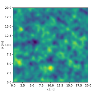
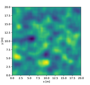
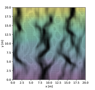
In more detail: a multivariate 20 m square master hydraulic conductivity field was generated using the GSTools package (Muller and Schuler, 2019) with an 0.1 m discretization length and geometric mean conductivity of $10^{-2}\ \mathrm{ms^{-1}}$. The (base 10) log hydrualic conductivity featured a multivariate Gaussian correlation structure with $\sigma^{2}_{\log K}$ = 0.5 and an exponential semivariogram with correlation length 0.5 m. From the 200 by 200 matrix representing the master conductivity field, the true conductivity field was derived by convolving against a uniform kernel with 0.8 m square support (represented by an 8 by 8 matrix). The smoothed conductivity field was derived by convolving against a uniform kernel with 1.6 m square support (represented by a 16 by 16 matrix). Both of the derived $\log K$ fields are shown in Figure 2. Both matrix convolutions, and all of the numerical analysis was performed in Python using the Numpy/Scipy ecosystem (Oliphant, 2007).

For each of the true and smoothed conductivity fields, a head field was derived by numerically solving the steady-state governing equation

$$\nabla\cdot\left(K(x,y)\nabla h(x,y)\right)=0,$$ (43)

subject to boundary conditions

$$h(x,0) = 0,$$ (44)

$$h(x,20) = 1,$$ (45)

$$\frac{\partial h}{\partial x}(0,y) = 0,$$ (46)

$$\frac{\partial h}{\partial x}(20,y) = 0,$$ (47)

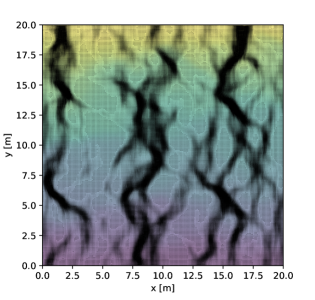
where $h(x,y)\ [\mathrm{m}]$ represents the hydraulic head at coordinate $(x,y)$. Solution was computed using second-order accurate finite difference techniques, employing the Scipy sparse matrix solver tools. The resulting head distributions are shown in Figure 2, and the relative smoothness of the $h$ field relative to the $\log K$ field, as posited when developing the CTRW-on-a-streamline approach, is plainly apparent.

From each head field, a velocity field, $\bm{v}(x,y)$ was determined by solving

$$\bm{v}(x,y)=\frac{K(x,y)\nabla h(x,y)}{\theta},$$ (48)

where $\theta=0.25$ was taken to be the spatially-uniform porosity, and cell center velocities were stored for each cell. These velocities are displayed as a quiver plot, again in Figure 2.

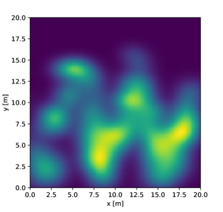
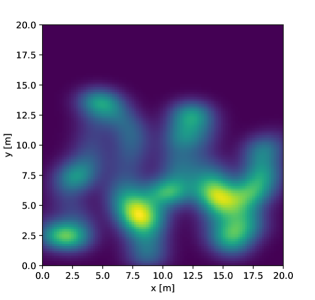
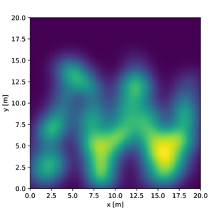
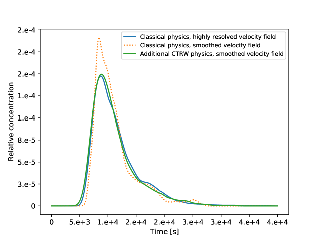
Finally, three different particle tracking simulations were performed, each by flux-weighted injection of 10000 particles along the top ($y=20$) boundary between $x=1$ and $x=19$. This was implemented by assigning weights to each cell adjacent to the relevant portion of the $y=20$ boundary according to the magnitude of the $y$-component of $\bm{v}$ at their respective cell centers. Subsequently, a weight-proportional portion of the 10000 particles was assigned to each of these border cells and these particles were initially positioned uniformly randomly within said cell. For each of the three simulations, particle tracking was performed using the CTRW-on-a-streamline approach and two events were recorded: (a) the location of all particles when $t=7\times 10^{3}$ s, and (b) the time of breakthrough of each particle at $y=0$. The three simulations were:

1. Classical physics on the highly resolved field: $f(t)=\delta(t)$, $\alpha_{t}=0.01$ m, with no MIMT.

2. Classical physics on the smoothed field: $f(t)=\delta(t)$, $\alpha_{t}=0.01$ m, with no MIMT.

3. Additional CTRW physics on the smoothed field: $f(t)$ inverse Gaussian with $\alpha_{l}=0.152$ m, $\alpha_{t}=0.01$ m, with no MIMT.

We see from qualitative comparison of the plume snapshots in Figure 3 and breakthrough curves in Figure 4 that the additional CTRW physics (in the form of $f(t)$) do capture much of the transport information that was lost when moving from the highly resolved to the smoothed field. This qualitative assessment is backed by comparison of the 2-norms (also known as Euclidian or Frobenius norms) of the difference between each of the two discretized concentration fields computed using the smoothed velocity field versus the true concentration field. The 2-norm of the error of the concentration field computed without additional CTRW physics is 1.59 times as large as that of the field computed with the additional physics. A similar picture emerges when the $\infty$-norms (largest absolute divergence) are compared. The $\infty$-norm of the no-additional-physics case is 1.68 times as large.

	True fields	Smoothed fields
$\bm{\log K}$ fields
Head and velocity fields

Figure 2: Illustration of log-hydraulic hydraulic conductivity, head, and velocity fields used in the simulations. In the first column are the spatially detailed fields treated as true. In the second column are spatially smoothed case fields that approximate the true fields in the first column. In the top row, log conductivity fields are shown, with lighter color indicating higher conductivity. In the bottom row, the corresponding hydraulic head fields are shown, with lighter color indicating greater head. Superimposed on each head field is a black quiver plot in which each arrow’s magnitude indicates the cell-center velocity for each cell in the discretization. (Because cell resolution is high, each arrow is quite small.)

	On true velocity field	On smoothed velocity field
With classical physics only
With additional CTRW physics

Figure 3: Plumes generated by kernel density estimation from the positions of simulated particles for the three simulation cases; brighter color indicates higher concentration. Plumes in the top row were generated by pure advection plus transverse diffusion, whereas the plume in the bottom row also featured advective scattering from inverse Gaussian $f$. The plume in the left column was simulated on the true velocity field, while those on the right were simulated on the smoothed field. The greater similarity between the true plume (top left) and the plume simulated using the smoothed velocity field plus additional CTRW physics (bottom right) versus the plume simulated using the smoothed velocity field alone (top right) is apparent.

Figure 4: Breakthrough curves at $y=0$ for each of the three simulations.

5 Summary and conclusion

We have presented a hybrid approach to modeling solute transport on velocity fields that are explicitly characterized at a coarse scale, but which contain small-scale physical heterogeneity and/or mass transfer leading to non-Fickian transport. The approach, which we call “CTRW-on-a-streamline” is a particle tracking technique that represents an advance of the current state of the art in which, for technical reasons, non-Fickian transport models or explicitly-delineated heterogeneous velocity fields are employed, but generally not both. Our approach separates the model parameters characterizing macroscopic flow, subscale advective heterogeneity, and mobile-immobile mass transfer, such that each can be directly specified a priori from available data, where relevant theory exists.

We have presented theory justifying our approach, formalized it in a set of governing equations that illustrate its connection to both classic CTRW and to subordination approaches, and operationalized it: listing an exact algorithm that one can implement. Finally, we presented a numerical demonstration of that implementation that supports the qualitative arguments for capturing small-scale heterogeneous advection validation with the single pdf, $f(r)$.

Acknowlegments

This paper does not concern a data set. Source code for the simulations is archived at https://doi.org/10.5281/zenodo.3558792. SKH holds the Helen Unger Career Development Chair in Desert Hydrogeology.

References

- Banton et al. [1997] Olivier Banton, Frederick Delay, and Gilles Porel. A New Time Domain Random Walk Method for Solute Transport in 1-D Heterogeneous Media. Groundwater, 35(6), 1997.
- Beaudoin and De Dreuzy [2013] A. Beaudoin and J. R. De Dreuzy. Numerical assessment of 3-D macrodispersion in heterogeneous porous media. Water Resources Research, 49(5):2489–2496, 2013. ISSN 00431397. doi: 10.1002/wrcr.20206.
- Benson and Meerschaert [2009] David A. Benson and Mark M. Meerschaert. A simple and efficient random walk solution of multi-rate mobile/immobile mass transport equations. Advances in Water Resources, 32(4):532–539, 2009. ISSN 03091708. doi: 10.1016/j.advwatres.2009.01.002.
- Berkowitz et al. [2006] B. Berkowitz, A. Cortis, M. Dentz, and H. Scher. Modeling non-Fickian Transport in Geological Formations as a Continuous Time Random Walk. Reviews of Geophysics, 44:RG2003, 2006. ISSN 0004-5411. doi: 10.1029/2005RG000178.
- Berkowitz et al. [2016] B. Berkowitz, I. Dror, S.K. Hansen, and H. Scher. Measurements and models of reactive transport in geological media. Reviews of Geophysics, 54(4), 2016. ISSN 19449208. doi: 10.1002/2016RG000524.
- Billingsley [1986] Patrick Billingsley. Probability and Measure. John Wiley & Sons, 2nd edition, 1986.
- Bodin [2015] Jacques Bodin. From analytical solutions of solute transport equations to multidimensional time-domain random walk (TDRW) algorithms. Water Resources Research, 51(3):1860–1871, 2015. ISSN 19447973. doi: 10.1002/2014WR015910.
- Bolster and Dentz [2012] D. Bolster and M. Dentz. Anomalous dispersion in chemically heterogeneous media induced by long-range disorder correlation. Journal of Fluid Mechanics, 695:366–389, 2012. ISSN 00221120. doi: 10.1017/jfm.2012.25.
- Carrera et al. [1998] Jesús Carrera, Xavier Sánchez-Vila, Inmaculada Benet, Agustín Medina, Germán Galarza, and Jordi Guinerà. On matrix diffusion: Formulations, solution methods and qualitative effects. Hydrogeology Journal, 6(1):178–190, 1998. ISSN 14312174. doi: 10.1007/s100400050143.
- Cirpka and Nowak [2003] Olaf A. Cirpka and Wolfgang Nowak. Dispersion on kriged hydraulic conductivity fields. Water Resources Research, 39(2):1–12, 2003. ISSN 00431397. doi: 10.1029/2001WR000598.
- Comolli et al. [2016] Alessandro Comolli, Juan J. Hidalgo, Charlie Moussey, and Marco Dentz. Non-Fickian Transport Under Heterogeneous Advection and Mobile-Immobile Mass Transfer. Transport in Porous Media, 115(2):265–289, 2016. ISSN 15731634. doi: 10.1007/s11242-016-0727-6.
- Cortis et al. [2004] Andrea Cortis, Claudio Gallo, Harvey Scher, and B. Berkowitz. Numerical simulation of non-Fickian transport in geological formations with multiple-scale heterogeneities. Water Resources Research, 40(4):1–16, 2004. ISSN 00431397. doi: 10.1029/2003WR002750.
- Cvetkovic and Haggerty [2002] V. Cvetkovic and R. Haggerty. Transport with multiple-rate exchange in disordered media. Physical Review E, 65(5):051308, 2002. ISSN 1063-651X. doi: 10.1103/PhysRevE.65.051308.
- Cvetkovic et al. [2016] V. Cvetkovic, A. Fiori, and G. Dagan. Tracer travel and residence time distributions in highly heterogeneous aquifers: Coupled effect of flow variability and mass transfer. Journal of Hydrology, 543:101–108, 2016. ISSN 00221694. doi: 10.1016/j.jhydrol.2016.04.072.
- Delay and Bodin [2001] Frederick Delay and Jacques Bodin. Time domain random walk method to simulate transport by advection-dispersion and matrix diffusion in fracture networks. Geophysical Research Letters, 28(21):4051–4054, 2001.
- Dentz and Berkowitz [2003] Marco Dentz and Brian Berkowitz. Transport behavior of a passive solute in continuous time random walks and multirate mass transfer. Water Resources Research, 39(5):1–20, 2003. ISSN 00431397. doi: 10.1029/2001WR001163.
- Edery et al. [2014] Yaniv Edery, Alberto Guadagnini, Harvey Scher, and Brian Berkowitz. Origins of anomalous transport in heterogeneous media: Structural and dynamic controls. Water Resources Research, 50:1490–1505, 2014. ISSN 00431397. doi: 10.1002/2013WR015111.
- Fetter [1999] C. W. Fetter. Contaminant Hydrogeology. Prentice-Hall, 1999.
- Gerke and van Genuchten [1993] H. H. Gerke and M. T. van Genuchten. A Dual-Porosity Model for Simulating the Preferential Movement of Water and Solutes in Structured Porous Media. Water Resources Research, 29(2):305–319, 1993.
- Gotovac et al. [2009] Hrvoje Gotovac, Vladimir Cvetkovic, and Roko Andricevic. Flow and travel time statistics in highly heterogeneous porous media. Water Resources Research, 45(7):W07402, 2009. ISSN 0043-1397. doi: 10.1029/2008WR007168.
- Haggerty and Gorelick [1995] Roy Haggerty and Steven M Gorelick. Multiple-rate mass transfer for modeling diffusion and surface reactions in media with pore-scale heterogeneity. Water Resources Research, 31(10):2383–2400, 1995.
- Haggerty et al. [2000] Roy Haggerty, Sean A. McKenna, and Lucy C. Meigs. On the late-time behavior of tracer test breakthrough curves. Water Resources Research, 36(12):3467–3479, 2000. ISSN 00431397. doi: 10.1029/2000WR900214.
- Hansen and Berkowitz [2014] S. K. Hansen and B. Berkowitz. Interpretation and nonuniqueness of CTRW transition distributions: Insights from an alternative solute transport formulation. Advances in Water Resources, 74:54–63, 2014. ISSN 03091708. doi: 10.1016/j.advwatres.2014.07.011.
- Hansen and Vesselinov [2018] S. K. Hansen and V. V. Vesselinov. Local Equilibrium and Retardation Revisited. Groundwater, 56(1):109–117, 2018. ISSN 17456584. doi: 10.1111/gwat.12566.
- Hansen et al. [2016] S. K. Hansen, B. Berkowitz, V. V. Vesselinov, D. O’Malley, and S. Karra. Push-pull tracer tests: Their information content and use for characterizing non-Fickian, mobile-immobile behavior. Water Resources Research, 52(12):9565–9585, 2016. ISSN 1093-474X. doi: 10.1111/j.1752-1688.1969.tb04897.x.
- Hansen et al. [2018] S. K. Hansen, C. P. Haslauer, O. A. Cirpka, and V. V. Vesselinov. Direct Breakthrough Curve Prediction From Statistics of Heterogeneous Conductivity Fields. Water Resources Research, 54(1):271– 285, 2018. ISSN 19447973. doi: 10.1002/2017WR020450.
- Kang et al. [2014] P. K. Kang, T. Le Borgne, M. Dentz, O. Bour, and R. Juanes. Impact of velocity correlation and distribution on transport in fractured media: Field evidence and theoretical model. Water Resources Research, 51:940–959, 2014. doi: 10.1002/2013WR014956.Received.
- Kreft and Zuber [1978] A. Kreft and A. Zuber. On the physical meaning of the dispersion equation and its solutions for different initial and boundary conditions. Chemical Engineering Science, 33(11):1471–1480, 1978. doi: 10.1016/0009-2509(78)85196-3.
- Margolin et al. [2003] Gennady Margolin, Marco Dentz, and Brian Berkowitz. Continuous time random walk and multirate mass transfer modeling of sorption. Chemical Physics, 295:71–80, 2003. ISSN 03010104. doi: 10.1016/j.chemphys.2003.08.007.
- Michalak and Kitanidis [2000] Anna M. Michalak and Peter K. Kitanidis. Macroscopic behavior and random-walk particle tracking of kinetically sorbing solutes. Water Resources Research, 36(8):2133–2146, 2000. ISSN 00431397. doi: 10.1029/2000WR900109.
- Moslehi and de Barros [2017] Mahsa Moslehi and Felipe P. J. de Barros. Uncertainty quantification of environmental performance metrics in heterogeneous aquifers with long-range correlations. Journal of Contaminant Hydrology, 196:21–29, 2017. ISSN 18736009. doi: 10.1016/j.jconhyd.2016.12.002.
- Muller and Schuler [2019] Sebastian Muller and Lennart Schuler. GeoStat-Framework/GSTools: Bouncy Blue (v1.0.1). 2019. doi: 10.5281/zenodo.2543658.
- Neretnieks [1980] Ivars Neretnieks. Diffusion in the rock matrix: An important factor in radionuclide retardation? Journal of Geophysical Research: Solid Earth, 85(B8):4379–4397, 1980.
- Nissan and Berkowitz [2019] Alon Nissan and Brian Berkowitz. Anomalous transport dependence on Péclet number, porous medium heterogeneity, and a temporally varying velocity field. Physical Review E, 99(3):1–11, 2019. ISSN 24700053. doi: 10.1103/PhysRevE.99.033108.
- Oliphant [2007] Travis E. Oliphant. Python for Scientific Computing. Computing in Science & Engineering, 9:10–20, 2007. doi: 10.1109/MCSE.2007.58.
- Painter et al. [2008] Scott Painter, Vladimir Cvetkovic, James Mancillas, and Osvaldo Pensado. Time domain particle tracking methods for simulating transport with retention and first-order transformation. Water Resources Research, 44(1):1–11, 2008. ISSN 00431397. doi: 10.1029/2007WR005944.
- Reimus and James [2002] Paul W. Reimus and Scott C. James. Determining the random time step in a constant spatial step particle tracking algorithm. Chemical Engineering Science, 57(21):4429–4434, 2002. ISSN 00092509. doi: 10.1016/S0009-2509(02)00396-2.
- Rubin [2003] Yoram Rubin. Applied Stochastic Hydrogeology. Oxford University Press, New York, 2003.
- Russian et al. [2016] Anna Russian, Marco Dentz, and Philippe Gouze. Time domain random walks for hydrodynamic transport in heterogeneous media. Water Resources Research, 52:3309–3323, 2016. ISSN 1093-474X. doi: 10.1002/2015WR018511.
- Schumer et al. [2003] Rina Schumer, David A. Benson, Mark M. Meerschaert, and Boris Baeumer. Fractal mobile/immobile solute transport. Water Resources Research, 39(10):n/a–n/a, 2003. ISSN 00431397. doi: 10.1029/2003WR002141.
- Srinivasan et al. [2010] G. Srinivasan, D. M. Tartakovsky, M. Dentz, H. Viswanathan, B. Berkowitz, and B. A. Robinson. Random walk particle tracking simulations of non-Fickian transport in heterogeneous media. Journal of Computational Physics, 229(11):4304–4314, 2010. ISSN 00219991. doi: 10.1016/j.jcp.2010.02.014.
- Tsang [1994] Chin-fu Tsang. Flow channeling in strongly heterogeneous porous media : A numerical study. Water Resources Research, 30(5):1421–1430, 1994.
- Tyukhova et al. [2016] Alina Tyukhova, Marco Dentz, Wolfgang Kinzelbach, and Matthias Willmann. Mechanisms of anomalous dispersion in flow through heterogeneous porous media. Physical Review Fluids, 1(7):1–12, 2016. ISSN 2469990X. doi: 10.1103/PhysRevFluids.1.074002.
- Uffink et al. [2012] Gerard Uffink, Amro Elfeki, Michel Dekking, Johannes Bruining, and Cor Kraaikamp. Understanding the Non-Gaussian Nature of Linear Reactive Solute Transport in 1D and 2D: From Particle Dynamics to the Partial Differential Equations. Transport in Porous Media, 91(2):547–571, 2012. ISSN 01693913. doi: 10.1007/s11242-011-9859-x.
- Zhang et al. [2013] Yong Zhang, Christopher T. Green, and Graham E. Fogg. The impact of medium architecture of alluvial settings on non-Fickian transport. Advances in Water Resources, 54:78–99, 2013. ISSN 03091708. doi: 10.1016/j.advwatres.2013.01.004.