Gamma-ray Blazar variability: New statistical methods of time-flux distributions

Abstract

Variable $\gamma$-ray emission from blazars, one of the most powerful classes of astronomical sources featuring relativistic jets, is a widely discussed topic. In this work, we present the results of a variability study of a sample of 20 blazars using $\gamma$-ray (0.1–300 GeV) observations from Fermi/LAT telescope. Using maximum likelihood estimation (MLE) methods, we find that the probability density functions that best describe the $\gamma$-ray blazar flux distributions use the stable distribution family, which generalizes the Gaussian distribution. The results suggest that the average behavior of the $\gamma$-ray flux variability over this period can be characterized by log-stable distributions. For most of the sample sources, this estimate leads to standard log-normal distribution ($\alpha=2$). However, a few sources clearly display heavy tail distributions (MLE leads to $\alpha<2$), suggesting underlying multiplicative processes of infinite variance. Furthermore, the light curves were analyzed by employing novel non-stationarity and autocorrelation analyses. The former analysis allowed us to quantitatively evaluate non-stationarity in each source — finding the forgetting rate (corresponding to decay time) maximizing the log-likelihood for the modeled evolution of the probability density functions. Additionally, evaluation of local variability allows us to detect local anomalies, suggesting a transient nature of some of the statistical properties of the light curves. With the autocorrelation analysis, we examined the lag dependence of the statistical behavior of all the $\{(y_{t},y_{t+l})\}$ points, described by various mixed moments, allowing us to quantitatively evaluate multiple characteristic time scales and implying possible hidden periodic processes.

1 Introduction

The class of active galaxies that emit profusely at radio frequencies are radio-loud galaxies. These galaxies often show the presence of kiloparsec (kpc) scale relativistic jets. If the jet is oriented towards the Earth, the relativistic effects become dominant such that the Doppler-boosted non-thermal emission makes the sources remarkably brighter over a wide range of electromagnetic frequencies. The emission is found to be more pronounced at higher energies, e.g., X-ray and $\gamma$-rays. These objects could also be the sources of neutrinos flying through the inter-galactic medium(see IceCube Collaboration et al., 2018a, b). In addition, the kpc scale jets seem to be most efficient cosmic particle accelerators, wherein the particles, mainly leptons, are accelerated to several orders of rest-mass electron energies. As a result, large amounts of accelerated high-energy particles become sources of incoherent synchrotron emission by decelerating into the ambient jet magnetic field, thereby making the extended jet “visible". These energetic particles might also up-scatter the surrounding synchrotron photons which they themselves produced (see Maraschi et al., 1992; Mastichiadis & Kirk, 2002) or low-energy electrons of external origins e.g., from the accretion disk (Dermer & Schlickeiser 1993), broad-line region (Sikora 1994), and dusty torus (Błażejowski et al. 2000), resulting in a large output of MeV–TeV emission.

Variability over minute to decade timescales is one of the characteristic, defining properties of blazars. Numerous studies in various energy bands and across all timescales have been conducted over the years using all available ground and space based instruments (see Rieger, 2019; Madejski, & Sikora, 2016; Bhatta et al., 2018). Particularly in the $\gamma$-ray regime, studies of power density spectra have shown that the statistical nature of the variability can well be described by a single power-law in the Fourier domain (see Bhatta & Dhital, 2020, and references therein); in some sources, applying continuous autoregressive models leads to the inference of breaks in the power spectra, possibly corresponding to characteristic timescales (Ryan et al., 2019). Indeed, time domain analysis of blazars serves as one of the most important tools to unravel the physical process occurring in the innermost regions around the central engines. The aim of this current work is to explore the statistical properties of the light curves in order to infer more fundamental mathematical properties of the process(es) driving the variability, such as linearity and stationarity. Moreover, as blazar variability timescales span a wide temporal range, i.e., from a few minutes to several decades, it is natural to conceive of the observed (total) flux variability as a combination of flux variability owing to individual stochastic processes occurring within the different sub-volumes of the parsec-scale accretion disk and kpc-scale relativistic jets. In such a scenario, it is an important question to ask whether such a combination is of an additive or a multiplicative nature. Several recent works on blazars show that the blazar flux distribution is well representated by a heavy tailed log-normal PDF. Particularly, the $\gamma$-ray fluxes of some of the brightest blazars have been found to follow log-normal distributions (see e. g. Bhatta & Dhital, 2020; Shah et al., 2018, and references therein). Such flux log-normality is often interpreted as an indication of the non-linearity in the multiplicative processes. In the context of AGN, it has been proposed that long-memory processes, such as flicker noise, originate due to the inward propagation of fluctuations in the mass accretion rates, which in turn create the rapid variability near the central region (see Lyubarskii, 1997). Magnetohydrodynamic (MHD) simulations of a thin disk around the black hole results in the observed log-normality along with the linear RMS-flux relations (Hogg & Reynolds, 2016). Similarly, in the statistical model of minijets-in-a-jet (see Giannios et al., 2009) isotropically oriented Doppler-boosted mini-jets are distributed over the span of the bulk relativistic flow. The total flux from the whole emission region is then of the log-normal form (Biteau & Giebels, 2012).

The skewness of the flux distribution suggests that the variability stems from multiplicative processes, which are associated in some models with the accretion disk. In this paper, we study the rms-flux relation and emphasize its link to Pareto distributions. The minijets-in-a-jet statistical model reconciles the fast variations and the statistical properties of the flux of blazars at very high energies.

As an attempt to understand the phenomenon of multi-timescale, multi-frequency variability in the sources, several emission models have been invoked; some of the widely discussed models include various magnetohydrodynamic instabilities in the turbulent jets (e.g. Bhatta et al., 2013; Marscher, 2014), shocks traveling down jets (e.g. Marscher & Gear, 1985; Spada et al., 2001), the aforementioned jets-in-a jet model (Giannios et al., 2009) and effects of jet orientation or geometric models (e.g. Larionov et al., 2016). In spite of the collaborative efforts across many instruments and observations, and in modeling and theory, the details of the processes shaping multi-timescale variability still remains debated. The importance of time domain analysis with a focus on constraining the nature of the variability can not be exaggerated as variability studies provide us with an excellent tool to probe the energetics of supermassive black hole systems.

In this work, we perform a statistical analysis of decade-long Fermi-LAT observations of 20 blazars that were presented in Bhatta & Dhital (2020). The source names, their 3FGL catalog names, source classifications, r.a., declinations, and redshifts are presented in columns 1, 2, 3, 4, 5 and 6, respectively, of Table 1. In Section 3, the details of the analyses methods carried out on the $\gamma$-ray light curves are discussed. The results and the discussions are presented in Section 4.

Table 1: General information about the sample FermiLAT blazars

Source name	Source class	3FGL name	R.A. (J2000)	Dec. (J2000)	Redshift ($z$)
W Comae	3FGL J1221.4+2814	BL Lac	$12^{\rm h}~{}21^{\rm m}~{}31\aas@@fstack{s}7$	$+28^{\circ}~{}13\arcmin~{}59\arcsec$	0.102
PKS 1502+106	3FGL J1504.4+1029	FSRQ	$15^{\rm h}~{}04^{\rm m}~{}25\aas@@fstack{s}0$	$+10^{\circ}~{}29\arcmin~{}39\arcsec$	1.84
4C+38.41	3FGL J1635.2+3809	FSRQ	$16^{\rm h}~{}35^{\rm m}~{}15\aas@@fstack{s}5$	$+38^{\circ}~{}08\arcmin~{}04\arcsec$	1.813
BL Lac	3FGL J2202.7+4217	BL Lac	$22^{\rm h}~{}02^{\rm m}~{}43\aas@@fstack{s}3$	$+42^{\circ}~{}16\arcmin~{}40\arcsec$	0.068
3C 279	3FGL J1256.1$-$0547	FSRQ	$12^{\rm h}~{}56^{\rm m}~{}11\aas@@fstack{s}1665$	$-05^{\circ}~{}47\arcmin~{}21\aas@@fstack{\prime\prime}523$	0.536
CTA 102	3FGL J2232.5+1143	FSRQ	$22^{h}32^{m}36.4^{s}$	$+11^{\circ}~{}43\arcmin~{}51\arcsec$	1.037
4C +21.35	3FGL J1224.9+2122	FSRQ	$12^{h}24^{m}54.4^{s}$	$+21^{\circ}~{}22\arcmin~{}46\arcsec$	0.432
Mrk 501	3FGL J1653.9+3945	BL Lac	$16^{h}53^{m}52.2167^{s}$	$+39^{\circ}~{}45\arcmin~{}36\aas@@fstack{\prime\prime}609$	0.0334
PKS 0454$-$234	3FGL J0457.0$-$2324	BL Lac	$04^{h}57^{m}03.2^{s}$	$-23^{\circ}~{}24\arcmin~{}52\arcsec$	1.003
1ES 1959+650	3FGL J2000.0+6509	BL Lac	$19^{h}59^{m}59.8521^{s}$	$+65^{\circ}~{}08\arcmin~{}54\aas@@fstack{\prime\prime}652$	0.048
PKS 1424$-$418	3FGL J1427.9$-$4206	FSRQ	$14^{h}27^{m}56.3^{s}$	$-42^{\circ}~{}06\arcmin~{}19\arcsec$	1.522
PKS 2155$-$304	3FGL J2158.8$-$3013	BL Lac	$21^{h}58^{m}52.0651^{s}$	$-30^{\circ}~{}13\arcmin~{}32\aas@@fstack{\prime\prime}118$	0.116
S5 0716+714	3FGL J0721.9+7120	BL Lac	$07^{h}21^{m}53.4^{s}$	$+71^{\circ}~{}20\arcmin~{}36\arcsec$	0.3
3C 66A	3FGL J0222.6+4301	BL Lac	$02^{h}22^{m}41.6^{s}$	$+43^{\circ}~{}02\arcmin~{}35\aas@@fstack{\prime\prime}5$	0.444
Mrk 421	3FGL J1104.4+3812	BL Lac	$11^{h}04^{m}273^{s}$	$+38^{\circ}~{}12\arcmin~{}32\arcsec$	0.03
ON +325	3FGL J1217.8+3007	BL Lac	$12^{h}17^{m}52.1^{s}$	$+30^{\circ}~{}07\arcmin~{}01\arcsec$	0.131
AO 0235+164	3FGL J0238.6+1636	BL Lac	$02^{h}38^{m}38.9^{s}$	$+16^{\circ}~{}36\arcmin~{}59\arcsec$	0.94
PKS 1156+295	3FGL J1159.5+2914	BL Lac	$11^{h}59^{m}31.8^{s}$	$+29^{\circ}~{}14\arcmin~{}44\arcsec$	0.7247
3C 454.3	3FGL J2254.0+1608	FSRQ	$22^{h}53^{m}57.7^{s}$	$+16^{\circ}~{}08\arcmin~{}54\arcsec$	0.859
3C 273	3FGL J1229.1+0202	FSRQ	$12^{h}29^{m}06.6997^{s}$	$+02^{\circ}~{}03\arcmin~{}08\aas@@fstack{\prime\prime}598$	0.158

2 Observations and data processing

The $\gamma$-ray observations of the sample blazar were obtained from the Large Area Telescope (LAT) onboard the Fermi Gamma-ray Space Telescope (Fermi) (Atwood et al., 2009). The telescope has a large effective area ($>8000\ cm^{2}$) to collect high energy photons coming from a wide field of view ($>$ 2 sr). Moreover, the instrument can resolve astronomical sources with a high angular resolution, that is, ($<3.5^{\circ}$ around 100 MeV and $<0.15^{\circ}$ above 10 GeV). To construct the source light curves, Pass 8 data fom the Fermi/LAT 3FG catalog were processed using Fermi Science Tools and following the standard procedures of the unbinned likelihood analysis. In particular, the photon events in the energy range 0.1–300 GeV classified as “evclass=128, evtype=3” were considered. A circular region of interest (ROI) of $10^{\circ}$ radius centered around each source was chosen; also, the zenith angle was limited to $<$ 90^∘ in order to minimize the contamination from the Earth. The Fermi Science Tools were used to perform analysis using the Fermi/LAT 3FG catalog, Galactic diffuse emission model and isotropic model for point sources. Moreover, the Galactic and extra-galactic diffuse $\gamma$-ray emission models gll_ iem v06.fit and iso_P8R2 SOURCE V6 v06.txt were also incorporated. To generate the weekly-binned light curves, a maximum-likelihood analysis, using the task gtlike, was performed on the photon events, and test statistics $\geq$ 10 (equivalently $\gtrsim 3\sigma$) (Mattox et al., 1996) were considered. For details on the data processing, refer to Bhatta & Dhital (2020).

3 Methodology and analysis

Following the extended methodology as explained in Duda (2018), we first normalized marginal distributions with a parametric distribution (log-stable here) as in copula theory (Durante et al., 2010), and then modeled the evolution of normalized variables, or joint distribution for autocorrelations. In both the cases, the PDFs were represented in terms of a polynomial basis.

3.1 Additive and multiplicative processes

In an additive process, the observed flux, say $X$, can be considered the sum of the fluxes produced at a number of randomly distributed smaller emission regions, i.e., $X=\sum_{i=1}^{N}x_{i}$. If the number of processes, assumed to be independent and identically distributed (i.i.d.) throughout the bulk emission region, becomes very large, i.e., $N\rightarrow\infty$, then by the central limit theorem, the total flux tends to follow a normal distribution. This distribution can also originate in stationary and linear systems with finite moments. In general, autoregressive processes, damped random walks, shot noise, and Brownian motion can be described as linear and additive processes. On the other hand, if the observed flux results from the multiplication of a large number of smaller fluxes, i.e., $X=\prod_{i=1}^{N}x_{i}$, then the integrated flux can follow a highly-skewed heavy tailed log-normal distribution. Such multiplicative processes are then ascribed to the non-linearity of the system. Multiplicative processes, e.g., the Volterra process (see Priestley, 1988), are widely discussed in the literature, such as in biological contexts by Mitzenmacher (2004), and in financial time series analysis by Zanette & Manrubia (2020).

3.2 Normalization with log-stable distribution

Figure 1: Some of the model probability distribution functions (PDF) and cumulative distribution functions (CDF) for stable distributions that are employed here to explore the $\gamma$-ray flux (logarithmized) distribution of the sample blazars. For the maximal value $\alpha=2$, it represents the normal distribution (Gaussian), and the skewness parameter $\beta$ has no effect. For $\alpha<2$, such a distribution has heavy tails following $\sim|x|^{-\alpha-1}$, and therefore posseses an infinite variance. According to the generalized central limit theorem (Gnedenko & Kolmogorov, 1949), the sum of a number of random variables with symmetric ($\beta=0$) distributions having power-law tails decreasing as $|x|^{-\alpha-1}$, where $0<\alpha<2$, will tend to be a stable distribution.

Figure 2: MLE Log-likelihood evaluations for $(\ln(x_{t}))$ sequences using the stable distribution with various fixed values of the $\alpha$ parameter for all 20 objects. Discontinuities correspond to large changes in the optimal value of $\beta$. The gray lines denote the fit yielding the most likely value of $\alpha$, which can be used to characterize a given object e.g., for classification, and in particular quantifying the tail type of its distribution. We can see that in particular the last five objects clearly lead to $\alpha<2$, suggesting infinite-variance heavy tails.

As in copula theory, for the methodology used here, it is convenient to first normalize flux values $(x_{t})$ to $y_{t}=f(x_{t})\in[0,1]$ having a nearly uniform distriubtion in the $[0,1]$ range (furthermore, Fig. 5 presents these normalized values $(y_{t})$). Here, $f$ ideally is the cumulative distribution function (CDF) that this sample comes from, and should represent the probability density averaged over the entire time period ($\approx 10$ years here). While this normalization could be performed by just sorting the values and assigning positions in order (the so-called empirical distribution function), using a parametric family would give a better understanding and suggest a universal behavior. In non-stationarity analysis we will additionally search for evolution of the probability density during this time period, as a correction to density used for normalization. In autocorrelation analysis, for pairs of values shifted by various lags, we will evaluate distortions from the uniform joint distribution on $[0,1]^{2}$.

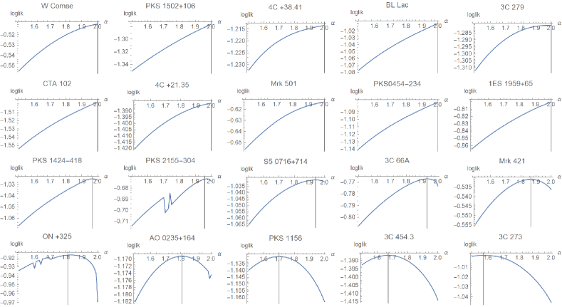
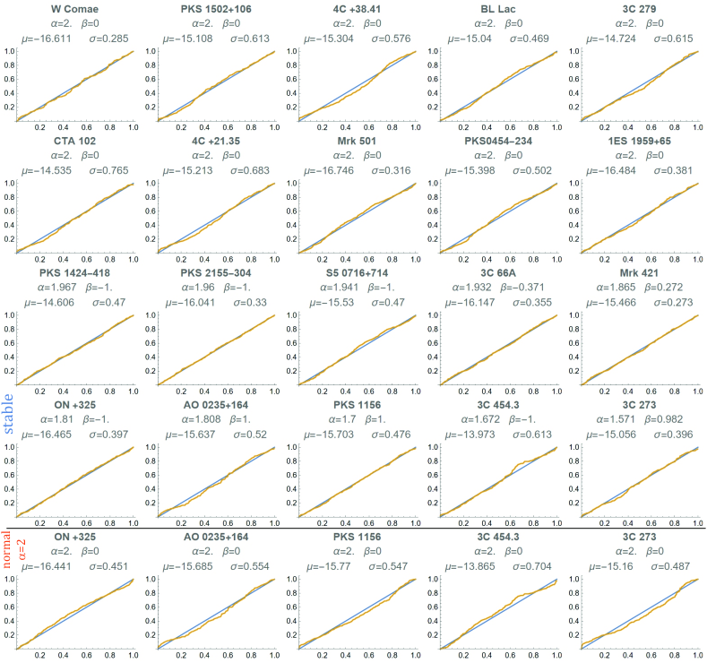
A standard assumption for the parametric distribution of this type of data, suggested by the central limit theorem for multiplicative processes, is the log-normal distribution: a Gaussian distribution for logarithmized values. To verify this assumption, we tested two larger families containing Gaussian distributions: exponential power distributions, $\rho(x)\sim\exp(-|x|^{\kappa})$, and stable distributions also containing heavy tails, $\sim|x|^{-\alpha-1}$ for $\alpha<2$. The highest log-likelihoods were achieved by using stable distributions for logarithmized values; hence they were applied for normalization (these evaluations are presented in Fig. 3).

The stable distribution (Borak et al., 2005) is defined by four parameters: $\mu,\sigma,\alpha,\beta$. As in the Gaussian distribution, it has a location parameter, $\mu\in(-\infty,\infty)$, and a scale parameter, $\sigma\in(0,\infty)$. Additionally it has a stability parameter, $\alpha\in(0,2]$. For $\alpha=2$ we get the standard Gaussian distribution; for $\alpha=1$ we get the Cauchy distribution with heavy tails following $1/x^{2}$. Generally for $\alpha\in(0,2)$ it has $|x|^{-\alpha-1}$ heavy tails, leading to infinite variance. This family also has a skewness parameter, $\beta\in[-1,1]$, which allows for some asymmetry in the distribution. However, its influence weakens when $\alpha$ approaches 2, and for $\alpha=2$ this parameter has no effect. Examples of probability distribution functions (PDF) and cumulative distribution functions (CDF) for some combinations of parameters of the stable distribution are presented in Fig. 1. It can be defined using the characteristic function $\varphi$:

$$\rho_{\mu\sigma\alpha\beta}(x)=\frac{1}{2\pi}\int_{-\infty}^{\infty}\varphi_{\mu\sigma\alpha\beta}(t)\,e^{-ixt}dt$$

$$\varphi_{\mu\sigma\alpha\beta}(t)=\exp\left(it\mu-|\sigma t|^{\alpha}(1-i\beta\,\textrm{sgn}(t)\tan(\pi\alpha/2)\right)$$ (1)

As the name suggests, these distributions have additional universality which might suggest a hidden mechanism — they are stable as per the central limit theorem, this time in its generalized version (Gnedenko & Kolmogorov, 1949). While addition of finite-variance i.i.d. random variables asymptotically leads to the Gaussian distribution, for infinite-variance variables such a summation usually leads to a stable distribution (at least for $\beta=0$). For some of the sources in our sample — those with $\alpha=2$ — there is good agreement with the log-stable distribution, suggesting a multiplicative process with finite variance; however the variance is infinite for the remaining sources (those with $\alpha<2$).

Figure 3: Visual evaluation of the level of agreement of MLE stable distributions for the 20 observed time series’ cumulative distribution functions (CDFs); the orange curve being equal to the blue diagonal would mean perfect agreement. Specifically, the original time series $(x_{t})$ was first logarithmized, then we performed an MLE (the most likely values of $\alpha,\beta,\mu,\sigma$ parameters are written in each panel). Then, the sequence $y_{t}=\textrm{CDF}_{\alpha\beta\mu\sigma}(\ln(x_{t}))$ was calculated using the CDF for parameters optimized for a given sequence. The orange curves are the sorted values of ${y_{t}}$, ideally from the uniform distribution which would yield the diagonal (blue). We can see that agreement between the curves is quite decent; the $\alpha=2$ cases correspond to just the log-normal distribution. However, as seen in Fig. 2, some objects have clearly lower values of $\alpha$, denoting heavier tails. The $\beta$ parameter denotes asymmetry and is limited to $[-1,1]$, which seems insufficient for a few sequences. The additional last row contains the same sources as the previous row, but normalized with log-normal distributions; we can see a larger discrepancy between the orange and blue curves. Disagreements near 0 and 1 suggest improper assumptions on the tail behavior of the probability density; disagreements near the center center suggest an improperly assumed body of the probability distribution

.

In the analysis presented here, the flux values $(x_{t})$ were first logarithmized, then for each individual object we performed a maximum likelihood estimation (MLE) of parameters of the stable distribution using Wolfram Mathematica software. To verify estimation of $\alpha$ and evaluate its accuracy, we also performed estimation with various fixed values of $\alpha$; those log-likelihoods are presented in Fig. 2. We can see that for some objects these fits suggest $\alpha<2$ and heavy tails, especially in 3C 273, 3C 454.3, PKS 1156+295, AO 0235+164, and ON +325.

We then performed normalization using cumulative distribution functions (CDF) of the most likely distributions: assuming a given sequence $(\ln(x_{t}))$ has led, by MLE, to parameters $(\alpha,\beta,\mu,\sigma)$, we calculated the sequence

$$y_{t}=\textrm{CDF}_{\alpha\beta\mu\sigma}(\ln(x_{t}))$$ (2)

which would be from the uniform distribution on $[0,1]$ if $(\ln(x_{t}))$ was exactly from this stable distribution.

Beside log-likelihood tests, we also performed a visual evaluation to test if such normalized variables $(y_{t})$ are from a nearly uniform distribution: by sorting them (empirical distribution) and comparing with the diagonal, which would be obtained for the uniform distribution. Fig. 3 presents such a visual evaluation, where we can see a relatively good agreement, especially at the boundaries corresponding to tails.

In this Figure, we also list the stable distribution parameters $\alpha,\beta,\mu,\sigma$ found via MLE. For most of the sequences we obtained $\alpha=2$, which means that indeed the log-normal distribution has turned out to be the best choice. However, the last few sequences in this Figure (they were ordered by $\alpha$) yielded lower values of $\alpha$ in this ML estimation, suggesting heavier tails. Parameters of such a ML estimation can be treated as features of objects, e.g., for classification purposes, especially the $\alpha$ parameter defining the type of tail of the distribution.

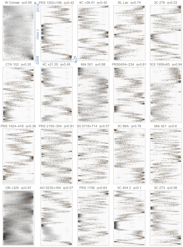
The normalized sequences $(y_{t})$ are later presented in Fig. 5 as dots, where we can see that in the horizontal direction they have a nearly uniform distribution. However, the local density evolves in the vertical direction corresponding to time, as is considered in non-stationarity analysis.

3.3 Modelling non-stationarity with polynomials of evolving contribution

After normalization, the variables $(y_{t})_{t=1..n}$ are from nearly-uniform distributions. Here we would like to model any distortions from this uniform distribution, such as its evolution for non-stationarity analysis, by representing this density as a polynomial and modelling its coefficients as discussed in Duda (2018).

For this purpose we could model the joint distribution of the pairs $\{(y_{t},t)\}$, with times $t$ rescaled to the range $[0,1]$, and predict the conditional distributions $\rho(y|t)$ using a polynomial model for their joint distributions. We performed 10-fold cross-validation tests of log-likelihood for such an approach, but it led to an inferior evaluation compared to an adaptive approach; hence we will focus only on the adaptive approach here, especially since it also provides evaluation of non-stationarity of the sequences.

We would like to model distortions from uniform density, $[0,1]$, (for normalized variables) as linear combinations using some basis $\{f_{j}:j\in B\}$, $B^{+}=B\backslash\{0\}$, $f_{0}=1$:

$$\rho(y)=\sum_{j\in B}a_{j}\ f_{j}(y)=1+\sum_{j\in B^{+}}a_{j}\ f_{j}(y).$$ (3)

As discussed in Duda (2018), these coefficients have similar interpretations as moments: $a_{1}$ as the expectation value, $a_{2}$ as the variance, $a_{3}$ as skewness, $a_{4}$ as kurtosis, etc. Using the orthornomal family of functions $\int_{0}^{1}f_{i}(y)f_{j}(y)dy=\delta_{ij}$, the mean-square error estimation is given by just averages of functions over the data sample $(y_{i})_{i=1..n}$:

$$a_{j}=\frac{1}{n}\sum_{i=1}^{n}f_{j}(y_{i})$$ (4)

We tested various orthornormal families including the trigonometric family, and generally the best results were obtained for (rescaled Legendre) polynomials: $f_{0},f_{1},f_{2},f_{3},f_{4}$ are correspondingly:

$$1,\sqrt{3}(2y-1),\sqrt{5}(6y^{2}-6y+1),$$

$$\sqrt{7}(20y^{3}-30y^{2}+12y-1),\ \text{and}\ (70y^{4}-140y^{3}+90y^{2}-20y+1)$$

For adaptivity we can replace the average in Eqn. (4) with an exponential moving average for some $\eta\in(0,1)$ forgetting rate:

$$a_{j}(t+1)=\eta\,a_{j}(t)+(1-\eta)f_{j}(y_{t})=a_{j}(t)+(1-\eta)(f_{j}(y_{t})-a_{j}(t)).$$ (5)

We estimate density $\rho_{t}(y)=\sum_{j\in B}a_{j}(t)\ f_{j}(y)$ for a given time $t$ based only on previous values, with exponentially weakening weights $\propto\eta^{\Delta t}=e^{\ln(\eta)\,\Delta t}$ for value $\Delta t$ time ago, allowing us to interpret $-1/\ln(\eta)$ as characteristic lifetime.

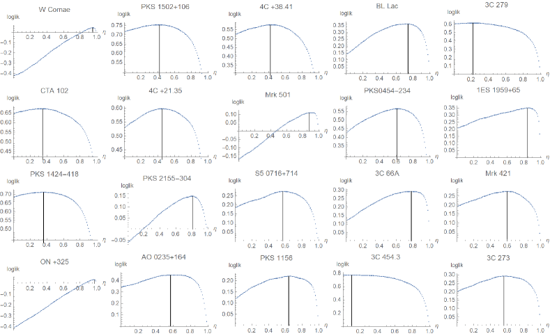
There remains a difficult question of choosing the rate $\eta$, which defines the strength of updates or lifetime, and which generally could also evolve. To find the optimal value of $\eta$ (fixed here), we searched the space of $\eta=0,0.01,\ldots,1$ for a fixed basis $B=\{0,1,2,3,4\}$, evaluating log-likelihoods: the average $\ln(\rho_{t}(y_{t}))$ for $\rho_{t}(y)=\sum_{j}a_{j}(t)\,f_{j}(y)$. However, the problem is that values of $\rho$, as a polynomial, sometimes get below zero; hence we need to reinterpret such negative predicted densities as small positives, in what is referred to as calibration: we instead used the log-likelihood as an average $\ln(\tilde{\rho}_{t}(y_{t}))$, where $\tilde{\rho}_{t}=\max(\rho_{t},\epsilon)/N$ and $N$ is a normalization constant to integrate to 1, and $\epsilon$ was arbitrarily chosen as 0.3 here.

The results of such a search for optimal values of $\eta$ using log-likelihood evaluations are presented in Fig. 4. While in financial time series, optimal values of $\eta$ are usually close to 1, here they can be very far from 1, suggesting strong non-stationarity — that is, this optimal value of $\eta$ can be treated as a feature characterizing non-stationarity of an object. The log-likelihoods obtained are relatively large: while a stationary density $\rho=1$ would have log-likelihood equal to 0, here the values can go up to $\approx 0.8$, corresponding to mean values $\exp(0.8)\approx 2.2$ times localization in the range $[0,1]$.

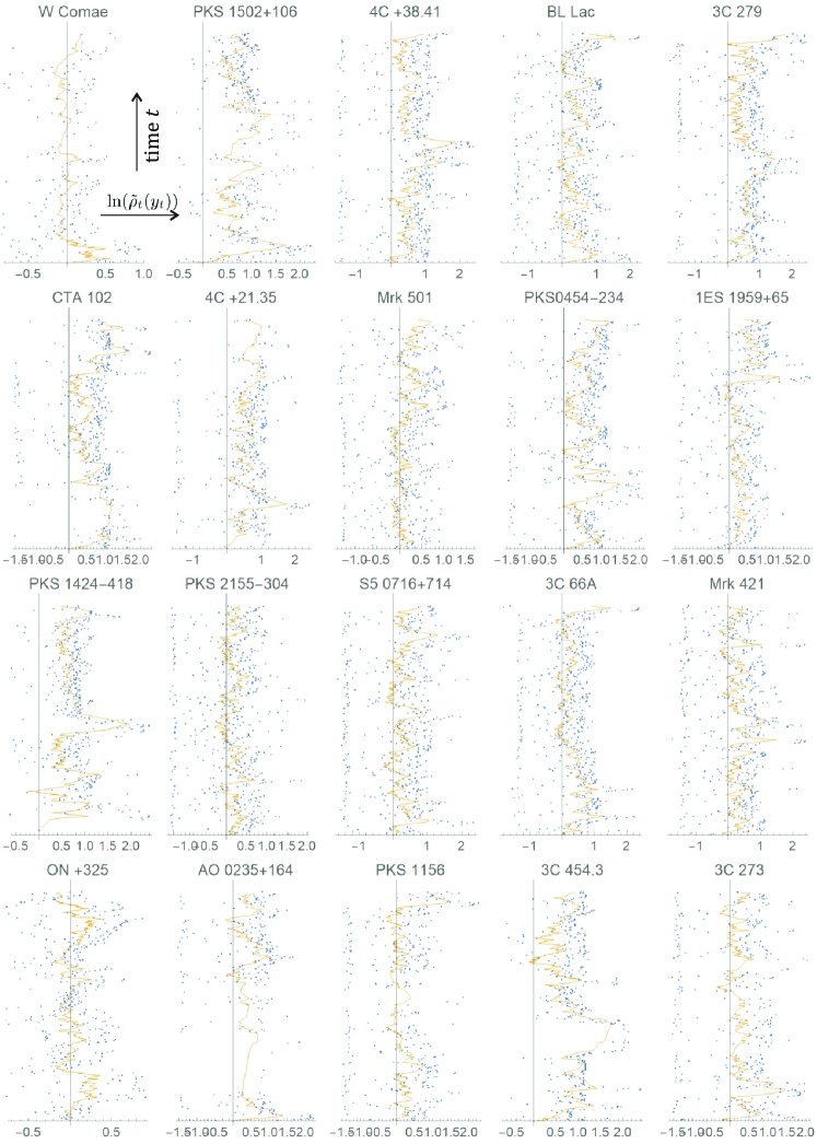
Finally the predicted evolving densities using the optimized values of $\eta$ are presented in Fig. 5, together with the $(y_{t})$ points. Their values (horizontal direction) average to a nearly uniform distribution; however, there are obvious clusters in their time evolution (vertical direction), exploited in the adaptive model discussed here, and with predictions visualized as density. Figs. 6 show the time non-uniformity of evaluation of such predictions: $\tilde{\rho}_{t}(y_{t})$ sequences (blue points), which smoothing (orange line), can be used to evaluate local variability.

The approach discussed here is optimized for fixed time differences between measured values, which is not exactly true forthe data analyzed here: we can see in Fig. 5 that density is constant between succeeding observations. Varying time difference could be included, e.g., by faster modification (lower $\eta$) for longer time differences, but such attempts did not lead to significant improvement of evaluation, and hence are not presented.

We could also use separate variables $\eta_{j}$ for each parameter $a_{j}$ and optimize them individually (also varying in time), modify the basis size and $\epsilon$ in calibration; we performed such initial tests, but we obtained nearly negligible improvement, so such tests are omitted here for simplicity. The results presented also did not include errors of values. They could be included, e.g., by replacing values with discretized sets of values weighted with probabilities ($f_{j}(y)\to\sum\textrm{Pr}(y)f_{j}(y)$), but such changes also yielded nearly negligible impact on results.

Figure 4: Search for optimal values of the $\eta$ parameter (independently for each source) for evaluation of non-stationarity: while the log-stable distribution obtained is averaged over a long period, the local probability distribution might evolve in time. For each normalized variable $y$ we found the time evolution of the coefficients $a_{1},a_{2},a_{3},{\rm and}a_{4}$ using an exponential moving average: $a_{j}(t+1)=\eta\,a_{j}(t)+(1-\eta)f_{j}(y_{t})$. The plots show the dependence of log-likelihood on $\eta$, without with the log-likelihood would be zero. We can see that in all but two cases (W Comae, and ON +325), we can essentially increase the log-likelihood by adjusting the parameters. Moreover, while e.g., in financial time series $\eta$ is usually $>0.99$, here the optimal values of $\eta$ can be much smaller, corresponding to extremely fast forgetting of these systems. Both the optimal value of $\eta$ (e.g. interpreted as lifetime following $-1/\ln(\eta)$) and the corresponding log-likelihood can be used as features of the object describing non-stationarity for example for classification purposes.

3.4 Autocorrelation analysis

We also performed autocorrelation analysis for each series $(y_{t})_{t=1..n}$ using a polynomial $(f_{j})$ basis similar to Duda (2021). We looked at pairs $(y_{t},y_{t+l})$ shifted by lag $l$, up to a maximal lag $m$ which was chosen here to be $m=100$ (weeks):

$$P_{l}=\{(y_{t},y_{t+l}):\textrm{ values in }t,t+l\textrm{ are available}\}\qquad\textrm{for}\qquad l=1,\ldots,m$$ (6)

The data available have a regular time difference (7 days); however, some values are missing. Hence we used all available pairs with a chosen lag, and such sets of pairs usually have size varying with lag (usually decreasing).

If uncorrelated, thanks to normalization, these pairs would be from a nearly uniform $\rho=1$ joint distribution on $[0,1]^{2}$. We would like to model distortion from this uniform distribution using a polynomial basis. Let us start with the product basis of orthornormal polynomials $(f_{j}(y)\cdot f_{k}(z))_{(j,k)\in B}$:

$$\rho_{l}(y,z)=1+\sum_{(j,k)\in B^{+}}a_{jk}(l)\ f_{j}(y)\,f_{k}(z)$$ (7)

Thanks to orthonormality we can use MSE estimation as in (4):

$$a_{jk}(l)=\frac{1}{|P_{l}|}\sum_{(y,z)\in P_{l}}f_{j}(y)\,f_{k}(z)$$ (8)

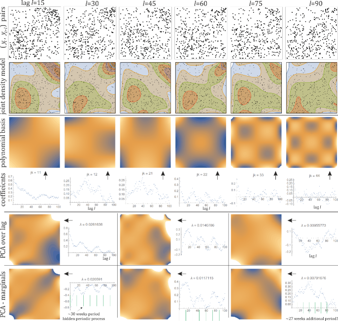
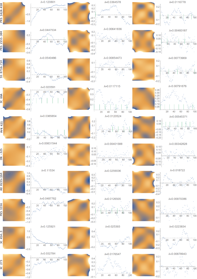
As with $f_{0}=1$, the coefficients $a_{j0}$ describe marginal distributions of the first variable, averaged over the second variable. Coefficients $a_{0k}$ describe the marginal distribution of the second variable. $a_{11}$ is the approximate dependence between their expected values, and has similar interpretation as the correlation coefficient. Furthermore, the coefficients $a_{kl}$ can be viewed as higher mixed moments; they describe the dependence between the $j$-th moment of the first variable and the $k$-th moment of the second variable. Their direct interpretation is through the density $f_{j}(y)f_{k}(z)$, which is presented in the third row of Fig. 7.

The top row of Fig. 7 contains examples of such pairs for 3C 66A. In the second row, we add isolines of joint density modeled using the $B=\{(j,k):j,k=0,\ldots,4\}$ polynomial basis. The third row presents densities $f_{j}(y)f_{k}(z)$ for some $(j,k)$ corresponding to $(1,1),(1,2),(2,1),(2,2),(3,3),{\rm and}(4,4)$. The fourth row shows the lag $l$ dependence $a_{jk}(l)$ for these six presented coefficients.

In the last two rows, we try to improve upon the above arbitrarily chosen basis by extracting features using PCA (principal component analysis) over lag $l$. Specifically, for each object we have $|B|=25$ sequences for $m=100$ lags. Averaging over lags we can find the $25\times 25$ covariance matrix $C_{j,k}$ and we can look at its few eigenvectors corresponding to the highest eigenvalues: $Cv=\lambda v$. Then we define a new basis $f_{v}=v\cdot(f_{jk}:(j,k)\in B)$ and corresponding sequence $a_{v}(l)=v\cdot(a_{jk}(l):(j,k)\in B)$ over lag $l$. For the three highest eigenvalues we present the contributions of $f_{v}$ to the joint density of $(y_{t},y_{t+l})$.

However, as discussed, these are highly non-stationary time series. If we wanted to focus here on statistical dependencies of values shifted by $l$, it would be beneficial to try to remove contributions from non-stationarity. There are many ways to realize this; for example we could use the evolved density modeled from non-stationarity analysis for the additional normalization, but such analysis would be model-dependent.

We used a simpler, more unequivocal approach instead: we subtracted the contributions of the (evolving) marginal distributions from the mixing terms:

$$\tilde{a}_{jk}=a_{jk}-a_{j0}\,a_{0k}\qquad\textrm{for}\quad k,j>0.$$ (9)

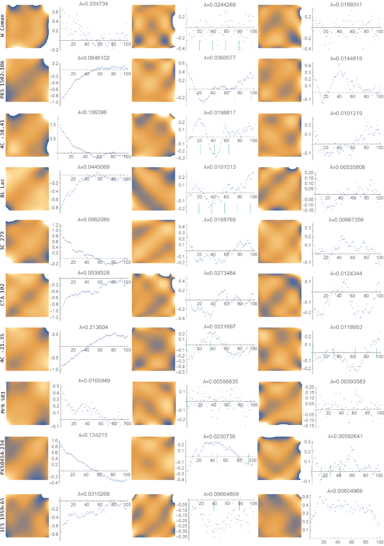
Then we could analogously perform PCA on $\tilde{a}_{jk}(l)$, leading to results presented in the bottom row of Fig. 7 and then analogously for all 20 objects in Figs. 8 and 9.

This way we obtain a few lag dependencies for each object, likely nearly independent thanks to PCA. As we can see in Fig. 8, 9 they show complex features, but often have clear minima-maxima structures, which could correspond to some characteristic time differences. Their deeper analysis might be an involved work and is planned for future research project; for example one could try to fit it with such a dependence for coupled pendulums. A first suggestion is that periodic processes should have alternating maxima/minima in fixed distances. Green lines show the results of such manual attempts, to be improved in a future work.

4 Results and Discussion

We carried out time series analysis on the $\gamma$-ray light curves of a sample of 20 blazars, employing several methods that aimed to constrain the statistical variability properties underlying the decade-long observations. In particular, the variable blazar flux distribution was investigated using log-stable PDFs. In addition, the light curves were analyzed using novel methods dealing with the statistical properties such as non-stationarity and autocorrelation. In this section, we discuss the results of the analyses and attempt to interpret them within the context of standard models of blazar variability and emission.

• The blazar $\gamma$-ray flux time series were fitted with general log-stable distributions parameterized by four parameters: location, variance, stability and asymmetry. The maximum likelihood estimation for most of the sources result in $\alpha$=2, which indicates a log-normal distribution consistent with our previous result in Bhatta & Dhital (2020, also see the references therein). Indeed a log-normal-like heavy-tailed flux distribution together with the linear RMS-flux relation could be a strong indication of the fact that the observed variability is driven by the multiplicative processes, which are non-linearly coupled over the large-scale jets. This then places constraints on the underlying mechanism producing the observed variable features in the light curves. For example, it likely rules out the role of independent shot-noise-like processes as they represent additive processes. In such a scenario, via a strong disk-jet connection, it is possible for the disk-based variations to make their way into the jet, propagate along the jet, and finally detected by the observer (e. g. see Giebels & Degrange, 2009). In the mini-jets scenario (see Biteau & Giebels, 2012), a power-law flux distribution can result owing to the transformation of the isotropic distribution of the boosts (of the mini-jets) in the frame of reference as they make a small angle to the line of sight.

  The analysis also revealed $\alpha<2$ heavy tails for some sources ($\rho(x)\sim|x|^{-\alpha-1}$), also an indication of multiplicative processes of infinite variance. This could be an important result that provides insights into the nature of $\gamma$-ray production in blazars, with an implication that the flux contributing to the higher end of the heavier tail of the PDF probably consists of large amplitude flaring events that could be of an different origin compared to the origin of the lower amplitude fluxes. Moreover, in practice it is not possible for the physical processes to realize infinite variances; this suggests that there could be a cut-off at the higher end of the flux distribution. Searching for the signatures of such cut-offs would be important because it places a strong constraint on the characteristic highest energies attainable in these systems. Such a characteristic energy would in turn shed light on the nature of the dominant particle acceleration scenario, e.g., shock waves and magnetic reconnection, contributing to the $\gamma$-ray production in the jets.

• One of the important results that the work revealed is that, although the PDF follows a log-stable distribution over a long period, it can display transient non-stationarity features, suggesting that the processes linked to the origin of variability are fast-forgetting. Such non-stationarity features, in the form of the fast changing PDFs, can be considered as statistical fluctuations in the long-term trend owing to local MHD instabilities either in the disc or in the turbulent jets (e.g. Calafut & Wiita, 2015; Marscher, 2014). Recently, transient non-stationarity in the form of variable PSD slopes was also reported in the X-ray observations of blazars, which were found to be consistent with short memory processes (Zhang et al., 2021; Bhattacharyya et al., 2020). The main parameters of the observed non-stationary are the forgetting rate $\eta$, which can be linked to lifetime $-1/\ln(\eta)$, and log-likelihood, which describes strength of localization. These parameters can represent some of the characteristics of intrinsic dynamics of the instability events. In addition, such quantities can be incorporated in the scheme of source classification.

• Novel auto-correlation analysis exploring the lag dependence of multiple mixed moments shows complex minima/maxima structures, and the timescales corresponding to these extrema are typically on the order of a few months. Recurrence analysis performed on the observations resulted in similar characteristic timescales, so-called trapping timescales, as reported in Bhatta et al. (2020). The timescales can be interpreted as some characteristic timescales associated with the jet processes. These timescales could be driven by the accretion disk-related timescales e.g., dynamical, thermal, or viscous timescales (see Czerny, 2006) in an AGN with a central black hole of mass on the order of$\sim 10^{8}-10^{9}M_{\odot}$; however, the timescales could be altered by the jet Lorentz factors. Additionally, the observed timescales can also be linked to Rayleigh-Taylor and Kelvin-Helmholtz instabilities developing at a disk-magnetosphere interface (Li & Narayan, 2004), or non-thermal (e.g. synchrotron and inverse-Compton) cooling timescales of the accelerated charged particle in the jet. Apart from aperiodic timescales, various jet and accretion disk-related instabilities can set up (quasi-) periodic oscillations as observed in the multi-frequency light curves of several blazars (see Bhatta, 2019, and references therein).

• Finally, it should be stressed that, although some of the results obtained here e. g., transient non-stationary features and heavy-tailed distribution, may have found a convenient interpretations in terms multiplicative and non-linear processes occurring at the turbulent relativistic jets, it is possible a broad range of stochastic processes to produce statistical properties similar to the observed time series, e. g., RMS-flux relation and log-normality. This makes it difficult to arrive at a common understanding of the physical model that drives the observed blazar variability. Furthermore, it appears that a robust correspondence between the observed properties, and the linearity/non-linearity and additive/multiplicative is yet to established (see Scargle, 2020, for a detailed discussion on the topic).

Data availability

The raw Fermi-LAT data used in this article can be accessed from the LAT server (https://fermi.gsfc.nasa.gov/cgi-bin/ssc/LAT/LATDataQuery.cgi). Furthermore, the processed data will be shared on reasonable request to the corresponding author.

Figure 5: Time-evolution of the estimated normalized density. In each plot the maximum likelihood forgetting rate obtained in Fig. 4 was used. The x-axis shows the normalized density range $[0,1]$. The y-axis is time from bottom to top (2008–2018, synchronized for all objects). The points indicate the estimated normalized flux, and if projected to the x-axis would correspond to a nearly uniform density. The grayscale values represent the model density given by, $\rho(y,t)=1+\sum_{j=1}^{4}f_{j}(y)a_{j}(t)$ for the values of $\eta$ optimizing the MLE (maxima in Fig. 4). The density uses the evolution $a_{j}(t+1)=\eta a_{j}(t)+(1-\eta)f_{j}(y_{t})$, and its moments are denoted by $j=\{1,2,3,4\}$. The gaps due to some of the missing values are filled with a constant density. Note that for some objects, such as 3C 279, PKS 2155$-$304, and Mrk 421, we can directly see oscillations.

Figure 6: The blue points show $\ln(\tilde{\rho}_{t}(y_{t}))$ in the horizontal direction and time evolution in the vertical direction. They average to log-likelihoods (maxima in Fig. 4), additionally allowing for evaluation of local time variability. The orange lines represent smoothing with an exponential moving average with rate 0.9. They can interpreted as local agreement with the models found; rapid decreases can be interpreted as anomalies.

Figure 7: Example of the autocorrelation analysis discussed for 3C 66A after normalization to nearly uniform variables $y_{t}=\textrm{CDF}(\ln(x_{t}))$. Row 1: $(y_{t},y_{t+l})$ pairs for various lags $l$. Row 2: their joint distribution modeled as $\rho(y,z)=1+\sum_{jk}a_{jk}\,f_{j}(y)f_{k}(z)$. Row 3: densities (orange are positive, blue are negative) of some the functions from the basis of orthonormal polynomials ($f_{j}(y)f_{k}(z)$) used for $(j,k)=(1,1),(1,2),(2,1),(2,2),(3,3),{\rm and}(4,4)$. Row 4: their corresponding coefficients $a_{jk}(l)$ for various lags $l=1,\ldots,100$. Row 5: bases found with principal component analysis (PCA), the densities of the corresponding functions, and their eigenvalues. Row 6: same as in row 5, but with earlier removal of contribution of marginal distributions $\tilde{a}_{jk}=a_{jk}-a_{j0}\,a_{0k}$, getting clearer signals only from dependencies between values shifted by lag $l$. This way we get decorrelated multiple lag dependencies for each object; we present a manual attempt at fitting alternating minima-maxima that suggest periodic processes.

Figure 8: Final plots for the first 10 sequences: PCA with removed marginal constributions as in row 6 of Fig. 7. Clear minima and maxima in lag dependence can be interpreted as characteristic timescales for a given object, with statistical interpretations presented in corresponding perturbations to joint densities $\rho(y_{t},y_{t+l})\approx 1+\sum_{v}a_{v}(l)f_{v}(y_{t},y_{t+l})$. Green lattices present attempts to manually deduce periodic processes as alternating minima/maxima in fixed distances, to be improved in future work.

Figure 9: Final plots for the last 10 sequences: PCA with removed marginal constributions as in row 6 of Fig. 7.

References

- Abdo et al. (2010) Abdo, A. A., Ackermann, M., Ajello, M., et al. 2010, ApJ, 722, 520
- Atwood et al. (2009) Atwood, W.B., Abdo, A.A. et al., 2009, ApJ, 697, 1071
- Bhatta et al. (2020) Bhatta, G., Pánis, R., & Stuchlík, Z. 2020, ApJ, 905, 160
- Bhatta & Dhital (2020) Bhatta, G., & Dhital, N. 2020, ApJ, 891, 120
- Bhatta (2019) Bhatta, G. 2019, MNRAS, 487, 3990
- Bhatta et al. (2018) Bhatta, G., Mohorian, M., & Bilinsky, I. 2018, A&A, 619, A93
- Bhatta et al. (2013) Bhatta, G., et. al. 2013, A&A, 558A, 92B
- Bhattacharyya et al. (2020) Bhattacharyya, S., Ghosh, R., Chatterjee, R., et al. 2020, ApJ, 897, 25
- Biteau & Giebels (2012) Biteau J., Giebels B., 2012, A&A, 548, A123
- Błażejowski et al. (2000) Błażejowski, M., Sikora, M., Moderski, R., & Madejski, G. M. 2000, ApJ, 545, 107
- Borak et al. (2005) Borak, S., Hardle, W., Weron, R., Stable distributions, Springer
- Calafut & Wiita (2015) Calafut, V. & Wiita, P. J. 2015, Journal of Astrophysics and Astronomy, 36, 255
- Camenzind & Krockenberger (1992) Camenzind M., Krockenberger M., 1992, A&A, 255, 59
- Czerny (2006) Czerny, B. 2006, Astronomical Society of the Pacific Conference Series, 360, 265
- Dermer & Schlickeiser (1993) Dermer, C. D., & Schlickeiser, R. 1993, ApJ, 416, 458
- Duda (2018) Duda, J., 2019, arXiv:1807.04119
- Duda (2021) Duda, J., Gurgul, H., & Syrek, R., 2021, Central European Journal of Operations Research, 1613-9178
- Durante et al. (2010) Durante, F., Sempi C., Copula theory: an introduction, Springer
- Giebels & Degrange (2009) Giebels B., Degrange B., 2009, A&A, 503, 797
- Giannios et al. (2009) Giannios, D., Uzdensky, D. A., & Begelman, M. C. 2009, MNRAS, 395, L29
- Gnedenko & Kolmogorov (1949) Gnedenko B.V., Kolmogorov A.N., 1949, Limit distributions for sums of independent random variables, Am. Math. Soc
- Hogg & Reynolds (2016) Hogg J. D., Reynolds C. S., 2016, ApJ, 826, 40
- IceCube Collaboration et al. (2018a) IceCube Collaboration, Aartsen, M. G., Ackermann, M., et al. 2018, Science, 361, eaat1378
- IceCube Collaboration et al. (2018b) IceCube Collaboration, Aartsen, M. G., Ackermann, M., et al. 2018, Science, 361, 147
- Larionov et al. (2016) Larionov, V. M., Villata, M., Raiteri, C. M., et al. 2016, MNRAS, 461, 3047
- Li & Narayan (2004) Li, L.-X., & Narayan, R. 2004, ApJ, 601, 414
- Lyubarskii (1997) Lyubarskii, Y. E. 1997, MNRAS, 292, 679
- Madejski, & Sikora (2016) Madejski, G. & Sikora, M. 2016, ARA&A, 54, 725
- Maraschi et al. (1992) Maraschi, L., Ghisellini, G., & Celotti, A. 1992, ApJ, 397, L5
- Mastichiadis & Kirk (2002) Mastichiadis, A., & Kirk, J. G. 2002, PASA, 19, 138
- Marscher (2016) Marscher, A. 2016, Galaxies, 4, 37
- Marscher (2014) Marscher, A. P. 2014, ApJ, 780, 87
- Marscher & Gear (1985) Marscher, A. P., & Gear, W. K. 1985, ApJ, 298, 114
- Mattox et al. (1996) Mattox, J. R., Bertsch, D. L., Chiang, J., et al. 1996, ApJ, 461, 396
- Mitzenmacher (2004) Mitzenmacher, M. (2004). A brief history of generative models for power law and log-normal distributions. Internet Math. 1, 226–251. doi: 10.1080/15427951.2004.10129088
- Priestley (1988) Priestley M. B., 1988, nlns.book
- Rieger (2019) Rieger, F. 2019, Galaxies, 7, 28
- Ryan et al. (2019) Ryan, J. L., Siemiginowska, A., Sobolewska, M. A., et al. 2019, ApJ, 885, 12
- Scargle (2020) Scargle J. D., 2020, ApJ, 895, 90. doi:10.3847/1538-4357/ab8d38
- Shah et al. (2018) Shah Z., Mankuzhiyil N., Sinha A., Misra R., Sahayanathan S., Iqbal N., 2018, RAA, 18, 141. doi:10.1088/1674-4527/18/11/141
- Sikora (1994) Sikora, M. 1994, ApJS, 90, 923
- Spada et al. (2001) Spada, M., Ghisellini, G., Lazzati, D., et al. 2001, MNRAS, 325, 1559
- Uttley, McHardy, & Vaughan (2005) Uttley P., McHardy I. M., Vaughan S., 2005, MNRAS, 359, 345. doi:10.1111/j.1365-2966.2005.08886.x
- Zanette & Manrubia (2020) Zanette, D. H. & Manrubia, S. 2020, Chaos, 30, 033104. doi:10.1063/1.5141837
- Zhang et al. (2021) Zhang, Z., Gupta, A. C., Gaur, H., et al. 2021, ApJ, 909, 103. doi:10.3847/1538-4357/abdd38