Revealing consensus and dissensus between network partitions
Abstract
Community detection methods attempt to divide a network into groups of nodes that share similar properties, thus revealing its large-scale structure. A major challenge when employing such methods is that they are often degenerate, typically yielding a complex landscape of competing answers. As an attempt to extract understanding from a population of alternative solutions, many methods exist to establish a consensus among them in the form of a single partition “point estimate” that summarizes the whole distribution. Here we show that it is in general not possible to obtain a consistent answer from such point estimates when the underlying distribution is too heterogeneous. As an alternative, we provide a comprehensive set of methods designed to characterize and summarize complex populations of partitions in a manner that captures not only the existing consensus, but also the dissensus between elements of the population. Our approach is able to model mixed populations of partitions where multiple consensuses can coexist, representing different competing hypotheses for the network structure. We also show how our methods can be used to compare pairs of partitions, how they can be generalized to hierarchical divisions, and be used to perform statistical model selection between competing hypotheses.
I Introduction
One of the most important tools in network analysis is the algorithmic division of an unannotated network into groups of similar nodes — a task broadly known as network clustering or community detection Fortunato (2010). Such divisions allow researchers to provide a summary of the large-scale structure of a network, and in this way obtain fundamental insight about its function and underlying mechanism of formation. Within this broad umbrella, many community detection methods have been developed, based on different mathematical definitions of the overall task Fortunato and Hric (2016). What most methods share in common is that they are based on some objective function defined over all possible partitions of the network, which if optimized yields the most adequate partition for that particular network. Another universal property of community detection methods is that when they are applied to empirical networks, they exhibit at least some degree of degeneracy, in that even if there exists a single partition with the largest score among all others, there is usually an abundance of other solutions that possess a very similar score, making a strict optimization among them somewhat arbitrary Good et al. (2010). This issue is compounded with the fact that instances of the community detection problem are generically computationally intractable, such that no known algorithm that guarantees the correct solution can perform substantially better than an exhaustive search over all answers Brandes et al. (2006); Decelle et al. (2011), which is not feasible for networks with more than very few nodes. As a consequence, most available methods rely on stochastic heuristics that give only approximations of the optimum, and end up being specially susceptible to the degenerate landscape, yielding different answers whenever they are employed.
In response to this inherent degeneracy, many authors have emphasized the need to collectively analyse many outputs of any given community detection method, not only the best scoring result Guimerà and Sales-Pardo (2009); Clauset et al. (2008); Calatayud et al. (2019); Riolo and Newman (2020). In this direction, one particularly interesting proposition is to recover the task of detecting a single partition, but doing so in a manner that incorporates the consensus over many different alternatives Strehl and Ghosh (2002); Topchy et al. (2005); Clauset et al. (2008); Goder and Filkov (2008); Lancichinetti and Fortunato (2012); Zhang and Moore (2014); Riolo and Newman (2020); Tandon et al. (2019). If most results are aligned with the same general solution, the consensus among them allow us in fact to profit from the degeneracy, since small distortions due to irrelevant details or statistical fluctuations are averaged out, leading to a more robust answer than any of the individual solutions. However, consensus clustering cannot provide a full answer to the community detection problem. This is because any kind of approach based on point estimates possesses an Achilles’ heel in situations where the competing answers do not all point in a cohesive direction, and instead amount to incompatible results. A consensus between diverging answers is inconsistent in the same manner as the mean of a bimodal distribution is not a meaningful representation of the corresponding population. Therefore, extracting understanding from community detection methods requires more than simply finding a consensus, as we need also to characterize the dissensus among the competing partitions. In fact, we need robust methods that give us a complete picture of the entire population of partitions.
Some authors have previously considered the problem of fully characterizing the landscape of possible partitions. Good et al Good et al. (2010) have used nonlinear dimensionality reduction to project the space of partitions in two dimensions, thereby revealing degeneracies. Closer to what is proposed in this work, Calatayud et al Calatayud et al. (2019) have used an ad hoc algorithm to cluster partitions, in order to determine how many samples are necessary to better characterize a distribution. Although these previous works effectively demonstrate the role of partition heterogeneity in empirically relevant situations, the approaches so far developed are implemented outside of a well-defined theoretical framework, and rely on many seemingly arbitrary choices, such as projection dimension, similarity function used, cluster forming criterion, etc. Because of this, it is difficult to interpret in simple terms the structures found by those methods, and also to evaluate if they are meaningful and statistically significant, or are merely artifacts of the provisional choices made.
In this work we develop a round set of methods to comprehensively characterize a population of network partitions, in a manner that reveals both the consensus and dissensus between them. Our methods start from the formulation of interpretable probabilistic generative models for arbitrary collections of partitions that are based on explicit definitions of the notion of unique group labelings and clusters of partitions. From these models, we are able to derive principled Bayesian inference algorithms that are efficient and effective at characterizing heterogeneous sets of partitions, according to their statistical significance. Importantly, our methods are nonparametric, and do not require a priori choices to be made, such as distance thresholds or even the number of existing clusters, with the latter being uncovered by our method from the data alone. Our method also bypasses dimensionality reduction Maaten and Hinton (2008); McInnes et al. (2018), as required by some data clustering techniques, and operates directly on a collection of partitions. Since it is grounded in a broader statistical framework, our method also allows potential generalizations, and principled comparison with alternative modelling assumptions.
We approach our characterization task by first providing a solution to the community label identification problem, which allows us to unambiguously identify groups of nodes between partitions even when their node compositions are not identical. This allows us to perform the basic (but until now not fully solved) task of computing marginal distributions of group memberships for each node in the network, and also leads naturally to a way of comparing partitions based on the maximum overlap distance, which has a series of useful properties that we demonstrate. Our method yields a simple way to characterize the consensus between a set of partitions, acting in a way analogous to a maximum a posteriori estimation of a categorical distribution. We highlight also the pitfalls of consensus estimation in community detection, which fails when the ensemble of solutions is heterogeneous. Finally, we provide a more powerful alternative, consisting of the generalization of our method to the situation where multiple consensuses are possible, such that groups of partitions can align in different directions. The identification of these partitions “modes” yields a compact and understandable description of the heterogeneous landscape of community detection results, allowing us to assess their consistency and weigh the alternative explanations they offer to the network data.
This work is divided as follows. We begin in Sec. II with a description of the label identification problem, which serves as a motivation for our approach on consensus clustering developed in Sec. III, based on the inference of what we call the random label model. In Sec. IV we discuss how we can extract consensus from network partitions via “point estimates,” and how this leads to inconsistencies in situations when the different partitions disagree. We then show how we can find both consensus and dissensus in Sec. V, by generalizing the random label model, thus obtaining a comprehensive description of multimodal populations of partitions, including how partitions may agree and disagree with each other. In Sec. VI we show how our ideas can be easily generalized to ensembles of hierarchical partitions, and finally in Sec. VII we show how our methods allow us to perform more accurate Bayesian model selection, which requires a detailed depiction of the space of solutions that our approach is able to provide. We end in Sec. VIII with a conclusion.
II The group identification problem in community detection
In this work we will focus on the approach to community detection that is based on the statistical inference of generative models Peixoto (2019). Although our techniques can be used with arbitrary community detection methods (or in fact for any data clustering algorithm), those based on inference lend themselves more naturally to our analysis, since they formally define a probability distribution over partitions. More specifically, if we consider a generative model for a network conditioned on a node partition , where is the group label of node , such that each network occurs with a probability , we obtain the posterior distribution of network partitions by employing Bayes’ rule,
| (1) |
where the prior probability of partitions, and is the model evidence. There are many ways to compute this probability, typically according to one of the many possible parametrizations of the stochastic block model (SBM) Holland et al. (1983) and corresponding choice of prior probabilities for their parameters. Since our analysis will not depend on any particular choice, we omit their derivations, and instead point the reader to Ref. Peixoto (2019) for a summary of the most typical alternatives. To our present goal, it is sufficient to establish that such a posterior distribution can be defined, and we have mechanisms either to approximately maximize or sample partitions from it.
The first central issue we seek to address is that for this class of problems the actual numeric values of the group labels have no particular significance, as we are interested simply in the division of the nodes into groups, not in their particular placement in named categories. This means that the posterior probability above is invariant to label permutations. More specifically, if we consider a bijective mapping of the labels , such that its inverse recovers the original labels, then a label permutation where , has the same posterior probability,
| (2) |
for any choice of . Very often this is considered an unimportant detail, since many inference methods break this label permutation symmetry intrinsically. For example, if we try to find a partition that maximizes the posterior distribution with a stochastic algorithm, we will invariably find one of the many possible label permutations, in an arbitrary manner that usually depends on the initial conditions, and we can usually move on with the analysis from there. Methods like belief-propagation Decelle et al. (2011), which can be employed in the special case where the model parameters other than the partition are known, yield marginal distributions over partitions that, due to random initialization, also break the overall label permutation symmetry, and yield a distribution centered around one particular group labelling. The same occurs also for some Markov chain Monte Carlo (MCMC) algorithms, for example those based on the movement of a single node at a time Peixoto (2014a); Riolo et al. (2017), which will often get trapped inside one particular choice of labels, since the swap of two labels can only occur if the respective groups exchange all their nodes one by one, a procedure that invariably moves the Markov chain through low probability states, and thus is never observed in practice. Although this spontaneous label symmetry breaking can be seen as a helpful property in these cases, strictly speaking it is a failure of the inference procedure in faithfully representing the overall label symmetry that does exist in the posterior distribution. In fact, this symmetry guarantees that the marginal posterior group membership probability of any node must be the same for all nodes, i.e.
| (3) |
where is the marginal distribution of the number of labels (nonempty groups), and we assume that the labels always lie in a contiguous range from to . Because of this, the true answer to the question “what is the probability of a node belonging to a given group?” is always an unhelpful one, since it is the same one for every node, and carries no information about the network structure. Far from being a pedantic observation, this is a problem we encounter directly when employing more robust inference methods such as the merge-split MCMC of Ref. Peixoto (2020a). In that algorithm, the merge and split of groups are employed as direct move proposals which significantly improve the mixing time and the tendency of the Markov chain to get trapped in metastable states, when compared to single-node moves. However, as a consequence, the merge and split of groups result in the frequent sampling of the same partition where two group labels have been swapped, after a merge and split. In fact, the algorithm of Ref. Peixoto (2020a) also includes a joint merge-split move, where the memberships of the nodes belonging to two groups are redistributed in a single move, which often results in the same exact partition, but with the labels swapped. Such an algorithm will rapidly cycle through all possible label permutations leading to the correct albeit trivial uniform marginal probabilities given by Eq. 3.
| \begin{overpic}[width=71.54768pt,trim=22.76228pt 22.76228pt 22.76228pt 22.76228pt]{polbooks-n0.jpg} \put(0.0,50.0){(a)} \end{overpic} | 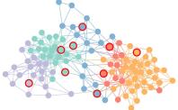 |
 |
 |
\begin{overpic}[width=130.08731pt,trim=0.0pt 0.0pt 0.0pt 0.0pt]{marginal-polbooks-nsamples100000.pdf} \put(-5.0,72.0){(b)} \end{overpic} | |
 |
||
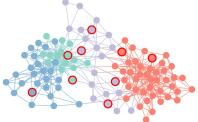
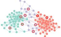
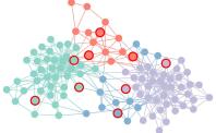
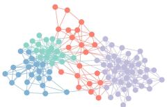
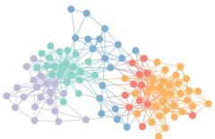
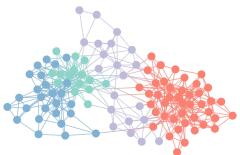
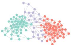
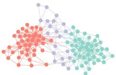
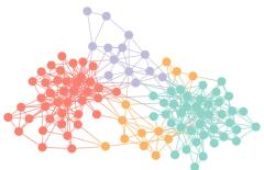
In Fig. 1 we show how the label permutation invariance can affect community detection for a network of co-purchases of political books Krebs , for which we used the Poisson degree-corrected SBM (DC-SBM) Karrer and Newman (2011), using the parametrization of Ref. Peixoto (2017), and the merge-split MCMC of Ref. Peixoto (2020a). Although the individual partitions yield seemingly meaningful divisions, they are observed with a random permutation of the labels, preventing an aggregate statistics at the level of single nodes to yield useful information.
At first we might think of a few simple strategies that can alleviate the problem. For example, instead of marginal distributions, we can consider the pairwise co-occurence probabilities , which quantify how often two nodes belong to the same group, and thus is invariant with respect to label permutations. However this gives us a large dense matrix of size which is harder to interpret and manipulate than marginal distributions — indeed the usual approach is to try to cluster this matrix Strehl and Ghosh (2002), by finding groups of nodes that have similar co-occurences with other nodes, but this just brings us back to the same kind of problem. Another potential option is to choose a canonical naming scheme for the group labels, for example by indexing groups according to their size, such that if , where is the number of nodes with group label . However this idea quickly breaks down if we have groups of the same size, or if the group sizes vary significantly in the posterior distribution. An alternative canonical naming is one based on an arbitrary ordering of the nodes and forcing the labels to be confined to a contiguous range, so that for whenever corresponds to a group label previously unseen for nodes . In this way every partition corresponds to a single canonical labeling, which we can generate before collecting statistics on the posterior distribution. Unfortunately, this approach is not straightforward to implement, since the marginal distributions will depend strongly on the chosen ordering of the nodes. For example, if the first node happens to be one that can belong to two groups with equal probability, whenever this node changes membership, it will incur the relabeling of every other group, and thus spuriously causing the marginal distribution of every other node to be broader, even if they always belong to the “same” group. It seems intuitive therefore to order the nodes according to the broadness of their marginal distribution, with the most stable nodes first, but since determining the marginal distribution depends on the ordering itself, it leads to a circular problem.
In the following we will provide a different solution to this problem, based on a generative model of labelled partitions, that is both satisfying and easy to implement, and allows us in the end to obtain marginal distributions in an unambiguous manner.
III Establishing consensus: The random label model
If we have as an objective the estimation of the marginal probability of node belonging to group , given partitions sampled from a posterior distribution, this is done by computing the mean
| (4) |
This is fully equivalent to fitting a factorized “mean-field” model on the same samples, given by
| (5) |
where is the probability of node belonging to group . Given the same partitions, the maximum likelihood estimate of the above model corresponds exactly to how we estimate marginal distributions, i.e.
| (6) |
Although this computation is common practice, it is important to note that this model is inconsistent with our posterior distribution of Eq. 1, since it is in general not invariant to label permutations, i.e. if we swap two labels and we have the same distribution only if for every node . Therefore, in order to tackle the label symmetry problem, we may modify this inference procedure, by making it also label symmetric. We do so by assuming that our partitions are initially sampled from the above model, but then the labels are randomly permuted. In other words, we have
| (7) |
where the intermediary partition is relabelled into with a uniform probability
| (8) |
where we make use of the symmetric indicator function
| (9) |
and where is the number of labels actually present in partition [not to be confused with the total number of group labels in the underlying model, since some groups may end up empty, so that ], and in total number of label permutations of . Now, inferring the probabilities from the model above involves finding a single underlying canonical labelling that is erased at each sample, but after it is identified allows us to obtain marginal distributions. This canonical labeling itself is not unique, since every permutation of its labels is equivalent, but we do not care about the identity of the labels, just an overall alignment, which is what the inference will achieve.
We proceed with the inference of the above model in the following way. Suppose we observe partitions sampled from the posterior distribution as before. Our first step is to infer the hidden labels from the posterior
| (10) |
with the marginal likelihood integrated over all possible probabilities , and given by
| (11) | ||||
| (12) |
where
| (13) |
is the number of relabelled partitions where node has hidden label , and we have used an uninformative prior
| (14) |
corresponding to a constant probability density for every node over a -dimensional simplex, each with volume , which is also equivalent to a Dirichlet prior with unit hyperparameters. Therefore, up to an unimportant multiplicative constant, we have that the posterior distribution of hidden relabellings is given by
| (15) |
where have assumed a uniform prior , which does not contribute to the above. We proceed by considering the conditional posterior distribution of a single partition ,
| (16) |
where is the label count excluding , and we have dropped the indicator function for conciseness, but without forgetting that must always hold. If we seek to find the most likely hidden labelling we need to maximize the above probability, or equivalently its logarithm, which is given by
| (17) |
up to an unimportant additive constant. The maximization involves searching through all possible relabellings of . Unfortunately, this number grows too fast for an exhaustive search to be feasible, unless the number of labels is very small. Luckily, as we now show, it is possible to re-frame the optimization, in a manner that exposes its feasibility. We begin by representing the mapping between the labels of and via the bijective function , chosen so that
| (18) |
Now, by introducing the matrix
| (19) |
we can express the log-likelihood as
| (20) |
Therefore, if we consider the matrix as the weighted adjacency matrix of a bipartite graph, where the group labels of and form the nodes on each partition (see Fig. 2), the above log-likelihood corresponds to the sum of the weights of the edges selected by . Finding such a bijection is an instance of a very well known combinatorial optimization problem called maximum bipartite weighted matching, also known as the assignment problem, which corresponds to finding a “matching” on a bipartite graph, defined as a subset of the edges that share no common nodes, such that the sum of the weights of the edges belonging to the matching is maximized. This corresponds precisely to the sum given in Eq. 20, where a given choice of corresponds to a particular matching. In particular we are interested in the unbalanced and imperfect version of the matching problem, where the number of groups on both sides might be different, and groups on either side might be left unmatched Ramshaw and Tarjan (2012), in which case for each unmatched group we give it a label of a new group. Luckily, fast polynomial algorithms for this problem have been long known. For example using the “Hungarian” or Kuhn–Munkres algorithm Kuhn (1955); Munkres (1957) this problem can be solved with a worst-case running time of , which is substantially better than an exhaustive search, rendering our approach not only feasible but efficient.
Having found the maximum of Eq. 20, we are still left with inferring the value of according to Eq. 15. But, as it is easy to verify, the likelihood is a monotonically decreasing function of . Therefore, since , this step amounts simply to choosing so that
| (21) |
Equipped with the above, we can summarize our whole inference algorithm as follows:
-
1.
We sample partitions from the posterior distribution .
-
2.
We initialize for every sample .
-
3.
For each sample , in random order, we obtain a new relabelling such that Eq. 20 is maximized.
-
4.
If any value of is changed during the last step, we repeat it, otherwise we stop and return .
-
5.
We update the inferred value of according to Eq. 21.
By the end of this algorithm, we are guaranteed to find a local maximum of Eq. 15, but not a global one, hence we need to run it multiple times and obtain the result with the largest posterior probability. However, we found that repeated runs of the algorithm give the same result the vast majority of cases we tried.111We offer a freely available reference C++ implementation of every algorithm described in this work as part of the graph-tool Python library Peixoto (2014b).
| Sampled | ||||
 |
 |
 |
|
|
| Relabelled | ||||
 |
 |
 |
|
|
| \begin{overpic}[width=216.81pt]{relabelled-marginal-polbooks-net.pdf} \put(0.0,55.0){(a)} \end{overpic} |
| \begin{overpic}[width=216.81pt]{relabelled-marginal-polbooks.pdf} \put(0.0,75.0){(b)} \end{overpic} |
Computationally, step 3 is the heart of the above algorithm, as it corresponds to the alignment of each partition with the rest. It takes time in the worst case, where is the total number of labels used, since for each partition we need time to compute the weights , and time to solve the maximum bipartite weighted matching problem. We can then use the final values of to easily obtain the marginal probabilities, via
| (22) |
Note that the above procedure is not much more computationally intensive than obtaining the marginals in the naive way, i.e. directly from the originally labelled partitions , which requires a time to record the label counts. It does, however, require more memory, with a total storage requirement, as we need to keep all partitions for the whole duration of the algorithm. In practice, however, we do not need to perform the whole procedure above for all partitions, as it is often sufficient to choose a relatively small subset of them, provided they give a good representation of the ensemble, and then we run steps 1 to 4 only on this subset. Based on that, we can simply process each remaining partition by simply finding its relabelling , updating the global label counts , and then discard the partition. Although this gives only an approximation of the optimization procedure, we find it works very well in practice, yielding results that are often indistinguishable from what is obtained with the full algorithm, while requiring less memory.
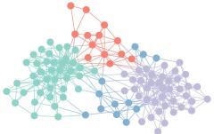
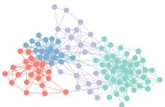
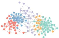
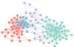
In Fig. 3 we show the partitions of the political books network considered in Fig. 1, but now relabelled according to the algorithm above. Despite groups changing size and composition, and the appearance and disappearance of groups, the unique labelling allows us to identify them clearly across partitions. In Fig. 4 these relabellings are used to obtain marginal distributions on the nodes, where we can say unambiguously with each frequency a node belongs to a given group.
III.1 The maximum overlap distance
The method described in this section serves as a principled way to disambiguate group labels in an ensemble of partitions, but the ideas articulated in its derivation also lead us to a way of comparing two partitions with each other in a general and meaningful way. Consider the situation where we employ the model above, but we have only partitions. In this case, without loss of generality, we can set one of them arbitrarily to correspond to the canonical labelling, and we seek to relabel the second one, by maximizing Eq. 20, which in this case simplifies to
| (23) |
where
| (24) |
is the so-called contingency table between partitions and , which quantifies how many nodes in group of belong to group of . Therefore, maximizing Eq. 23 is equivalent to finding the bijection so that with and maximize the partition overlap
| (25) |
which counts how many nodes share the same label in both partitions. Therefore, incorporating our inference procedure leads to the maximum overlap distance
| (26) |
This quantity has a simple interpretation as the minimal classification error, i.e. the smallest possible number of nodes with an incorrect group placement in one partition if the other is assumed to be the correct one. This measure has been considered before in Refs. Meilă and Heckerman (2001); Meilǎ (2005); Meilă (2007), but here we see its derivation based on a probabilistic generative model. In appendix A we review some of its useful properties.
IV Consensus as point estimates
The explicit objective of community detection, like any data clustering method, is to find a partition of the nodes of a network, in a manner that captures its structure in a meaningful way. However, instead of a single partition, the inference approach gives us a distribution of partitions, which ascribes to every possible division of the network a plausibility, reflecting both our modelling assumptions as well as the actual structure of the network. In order to convert this information into a single partition “point estimate” we have to be more specific about what we would consider a successful outcome, or more precisely how we define the error of our estimate. A consistent scenario is to assume that our observed network is indeed generated from our model where is the true partition we are trying to find. In order to quantify the quality of our inference we need to specify an error function that satisfies
| (27) |
Based on a choice for this function, and since we do not really have access to the true partition , our best possible estimate from the posterior distribution is the one which minimizes the average error over all possible answers, weighted according to their plausibility, i.e.
| (28) |
Therefore, it is clear that our final estimate will depend on our choice of error function , and hence is not a property of the posterior distribution alone. In statistics and optimization literature the function is called a “loss function,” and it determines the ultimate objective of the inference procedure.
In addition to producing a point estimate , it is also useful for our inference procedure to yield an uncertainty value , which quantifies how sure we are about the result, with indicating perfect certainty. Such choices are not unique, as there is often multiple ways to characterize the uncertainty or how broad is a distribution. But as we will see, the choice of the error function allows us to identify what are arguably the simplest and most direct options.
In the following we to consider simple choices of the error function, and investigate how they compare to each other in the inference results they produce.
IV.1 Maximum a posteriori (MAP) estimation
Arguably the simplest error function we can use is the indicator function (also called the “zero-one” or “all-or-nothing” loss)
| (29) |
which would separate the true partition completely from any other, without differentiating among wrong ones. Inserting this in Eq. 28, we obtain the maximum a posteriori (MAP) estimator
| (30) |
which is simply the most plausible partition according to the posterior distribution. The corresponding uncertainty for this estimate is simply , such that if we are maximally certain about the result. Despite its simplicity, there are several problems with this kind of estimation. Namely, the drastic nature of the error function completely ignores partitions which may be almost correct, with virtually all nodes correctly classified, except very few or in fact even one node placed in the incorrect group. We therefore rely on a very strong signal in the data, where the true partition is given a plausibility that is larger than any small perturbation around it, in order to be able to make an accurate estimation. This puts us in a precarious position in realistic situations where our data are noisy and complex, and does not perfectly match our modelling assumptions. Furthermore the uncertainty is in most cases difficult to compute, as it involves determining the intractable sum which serves as a normalization constant for (although we will consider approximations for this in Sec. VII). Even if computed exactly, typically we will have approaching the maximum value of one, since very few networks have a single partition with a dominating posterior probability.
IV.2 Maximum overlap consensus (MOC) estimation
As an alternative to the MAP estimation, we may consider a more relaxed error function given by the overlap distance
| (31) |
which counts the number of nodes correctly classified when compared to the true partition. With this function, from Eq. 28 we obtain the maximum marginal estimator
| (32) |
with
| (33) |
being the marginal posterior distribution for node . The uncertainty in this case is then simply the average of the uncertainty for each node, . Since this estimator considers the average over all partitions instead of simply its maximum, it incorporates more information from the posterior distribution. Nevertheless, we encounter again the same problem we have described before, namely that due to label permutation invariance the marginal distribution will be identical for every node, and this estimator will yield in fact useless results. We can fix this problem by employing instead the maximum overlap distance of Eq. 26 as an error function , leading to the estimator
| (34) |
Performing the maximization yields now a set of self-consistent equations,
| (35) |
with the marginal distributions obtained over the relabeled partitions,
| (36) |
where the relabeling is done in order to maximize the overlap with
| (37) |
Like before, the uncertainty is given by . In practice we implement this estimator by sampling a set of partitions from the posterior distribution and then performing the double maximization
| (38) | ||||
| (39) |
where in the last equation we have that is the contingency table between and . The solution of Eq. 38 is obtained by simply counting how often each label appears for each node and then extracting the label with the largest count, and Eq. 39 is once more an instance of the maximum bipartite weighted matching problem. The overall solution can be obtained by simple iteration, starting from an arbitrary choice of , and then alternating between the solution of equation Eq. 39 and using its result to solve Eq. 38, until no longer changes. This guarantees a local optimum of the optimization problem, but not necessarily a global one, therefore this algorithm needs to be repeated multiple times with different initial conditions, and the best result kept. Since it involves the relabelling over all partitions, the overall algorithmic complexity of a single iteration is .
Note that the marginal distributions obtained via Eq. 36 with the MOC estimator are not necessarily the same as those obtained by inferring the random label model considered previously. This is because while the MOC calculation attempts to find a single partition with a maximum overlap to all samples, inferring the random label model amounts to finding the most likely marginal distribution compatible with all samples, irrespective of its maximum. Although in many cases these two calculations will give similar answers, they are not equivalent.
IV.3 Error functions based on the contingency table
In principle, we can make a variety of other choices for error functions. A particular class of them are those based on the contingency table between partitions, using concepts from information theory. These error functions are not based on an explicit labeling or alignment of partitions, but instead focus on the joint probability of labels in both partitions being compared. A popular function of this kind is the variation of information (VI) Meilă (2003), which is defined as
| (40) |
with being the contingency table between and , and are the group sizes in both partitions. We can use VI as an error function by setting
| (41) |
As detailed in Ref. Meilă (2003), VI is a dissimilarity function that fulfills many desirable formal properties, including triangle inequality, making it a proper metric distance (like the maximum overlap distance). Another possible alternative consists of using the reduced mutual information (RMI) Newman et al. (2020), as done by Riolo and Newman Riolo and Newman (2020), with
| (42) |
where
| (43) |
with being the total number of contingency tables with fixed row and column sums, which we omit here for brevity (see Ref. Newman et al. (2020) for asymptotic approximations). The negative sign used in the definition of is because RMI is a similarity function, which takes its maximum value when and are identical, unlike VI, which is a dissimilarity that takes its minimum value of zero in the same case. RMI can be seen as a correction to mutual information, which fails as an appropriate similarity function in key cases. It is based on a nonparametric minimum description length encoding of both partitions, which quantifies the amount of information required to describe them if the contingency table is known, together with the necessary information required to describe the contingency table itself.
In either of the above cases, our point estimate consists of minimizing the sum of the error function over samples from the posterior distribution, according to Eq. 28. Unlike the indicator and the maximum overlap distance, the above loss functions are more cumbersome to optimize, with the overall optimization itself amounting to a nonconvex clustering problem of its own. Therefore we can use some of the same algorithms we use to perform community detection in the first place, with a good choice being the merge-split MCMC of Ref. Peixoto (2020a), which we have used in our analysis.
IV.4 Consensus point estimates are inconsistent for heterogeneous distributions
Our aim is not to list or perform an exhaustive comparison between all possible error functions, but instead to focus on the fact that they do not always yield the same answer. Although there is only one way with which all partitions in an ensemble can be identical, there are many ways in which they can be different. While the various error functions allow us to extract a form of consensus between differing partitions, they each achieve this based on different features of the population. Therefore, for partition ensembles with sufficiently strong heterogeneity, the different estimators may give conflicting answers. Such a disagreement can signal an arbitrariness in the inference procedure, and our inability of summarizing the population in a simple manner. We illustrate this problem with a few simple examples.
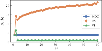
We consider first a simple artificial scenario with strong heterogeneity, composed of independently sampled partitions of nodes, where to each node is sampled a group label uniformly at random from the interval . Indeed, in this example there is no real consensus at all between partitions. Intuitively, we might expect the estimated consensus between such fully random partitions to be a sort of “neutral” partition, in the same way the average of a fully isotropic set of points in Cartesian space will tend towards the origin. However, all consensus estimators considered previously behave very differently from each other in this example. In Fig. 5 we compare the effective number of groups obtained for each point estimate, with
| (44) |
being the group label entropy. Arguably, the estimator that behaves the closest to the intuitive expectation just mentioned is VI, which for yields a consensus partition composed of a single group, . The MOC estimator yields instead a partition into groups, which itself is hard to distinguish from a random partition sampled from the original ensemble. This is because the marginal distributions obtained by Eq. 36 will be close to uniform, even after the label alignments of Eq. 39 are achieved, such that the maximum chosen by Eq. 38 will be determined by small quenched fluctuations in the partition ensemble. Finally, the RMI estimate yields consensus partitions with a number of groups that increases with the number of samples . This is because the RMI estimate tends to find the overlaps between partitions, i.e. sets of nodes that tend to occur together in the same group across many partitions Riolo and Newman (2020). In our random case, two nodes belong to the same group due to pure coincidence, therefore the probability of this happening for a large set of nodes decreases for larger , thus making the overlapping sets progressively smaller, and leading to a larger number of groups in the consensus. Inspecting any of the obtained point estimates in isolation, it would be difficult to get a coherent picture of the underlying ensemble, since none of them allow us to distinguish between an ensemble concentrated on the point estimate, or the maximally heterogeneous situation we have just considered. If we would consider instead the uncertainty of the MOC estimate (which yields for ), or even more explicitly the marginal distributions of Eq. 36 (or those of the inferred random label model of Sec. III), we would see that they are very broad, matching closely the true random distribution. But nevertheless, none of the point estimates by themselves can reveal this information.
 |
| MAP () and VI estimates |
 |
| MOC estimate () |
 |
| RMI estimate |
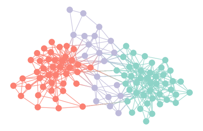
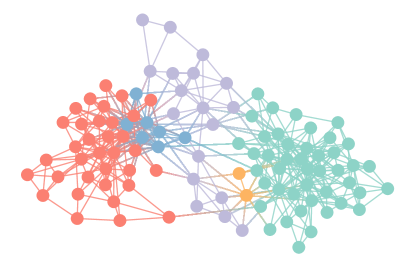
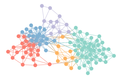
We further illustrate the discrepancy issue with a more realistic example where we can see both agreements and disagreements between the different estimates. In Fig. 6 we show the estimates obtained for the same political books network considered previously, again using the DC-SBM to obtain a posterior distribution of partitions. We observe, rather curiously, that the MAP estimate coincides perfectly with the VI estimate, but gives a different result from the MOC and RMI estimates. The MAP/VI estimates separate the network into three groups, which in this context can be understood as types of books describing “liberal” and “conservative” politics, and “neutral” books not taking any side. The MOC estimate further divides the “liberal” category into a new subgroup, and somewhat strangely at first, singles out two “neutral” books into their own category. As can be seen in Fig. 4, the reason for this is that the posterior distribution exhibits a possible subdivision of the neutral group into two, however it is only these two nodes that happen to belong to this subdivision with the highest probability. The RMI estimate also yields a division into five groups, but the two extra groups have a larger size when compared to the MOC result. In view of the behavior seen for the fully random example considered earlier, the discrepancies raise some doubts about what is the most faithful division. Are the MOC and RMI arbitrary divisions due to the randomness of the posterior distribution or do they point to a meaningful summary? Are the MAP/VI estimates being too conservative about the structure of the posterior distribution?
 |
 |
| MAP (), MOC () and VI estimates | RMI estimate |
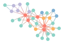
With some other networks, the discrepancy between estimators can be even stronger, making such questions even harder to answer. In Fig. 7 we show the results for Zachary’s karate club network Zachary (1977), again using the DC-SBM. In this case, the MAP, MOC and VI estimators yield the same division of the network into a single group, whereas the RMI estimate yields a partition into five groups, following no clear pattern. None of the estimates resemble the putative division for this network in two assortative communities.
Despite the partial agreement between some of the estimates in the examples above, the disagreements still raise obvious interpretation questions. Here we argue that this discrepancy cannot be resolved simply by trying alternative ways to form a consensus, since trying to summarize a whole distribution with a point estimate is in general an impossible task, and therefore we need instead a way to also characterize the dissensus between partitions, by exposing also the existing heterogeneity of the posterior distribution.
To some extent, the characterization of dissensus is already achieved by the random label model of Sec. III, since it attempts to describe the posterior distribution via marginal probabilities, rather than just a point estimate, and therefore can convey how concentrated it is. However, because this model assumes the group membership of each node to be independent, it still hides a significant fraction of the potential heterogeneity in the ensemble, which can come from the correlation between these memberships. In the next section we will generalize this approach to the situation where the posterior distribution is multimodal, so that multiple consensuses are simultaneously possible. We will see how this allows us to extract a more complete and coherent picture of distributions of partitions.
V Extracting dissensus between partitions
We aim to characterize the discrepancy between partitions by considering the possibility of several possible consensuses that only exist between a subset of the partitions. This corresponds to the situation where the inference procedure can yield substantially different explanations for the same network. We do so by modelling the posterior distribution of partitions with a mixture model, where each partition can belong to one of clusters — which we call “modes” to differentiate from the groups of nodes in the network. Inside each mode the partitions are generated according to the same random label model considered before, but with different parameters. More specifically, a partition is sampled according to
| (45) |
where
| (46) |
is the relative size of mode , with , and inside a mode the partitions are sampled according to the random label model,
| (47) |
with the hidden labels generated according to
| (48) |
where is the probability that a node has group label in mode , and finally a random label permutation chosen uniformly at random,
| (49) |
Naturally, we recover the original random label model for .
We perform the inference of the above model by considering the mode label as a latent variable, which yields a joint probability together with the original and relabelled partitions
| (50) |
If we now observe partitions sampled from the SBM posterior distribution, we assume that each one has been sampled from one of the modes, so that for each observed partition we want to infer its relabelled counterpart together with its originating mode, i.e. . The joint posterior distribution for these pairs, together with the total number of modes , and the number of groups in each mode, is given by
| (51) |
where the relabelling probability is given by
| (52) |
and with the marginal likelihood obtained by integrating over all possible probabilities for each mode,
| (53) | ||||
| (54) |
with being the number of samples that belong to mode , the total number of group labels in mode , and are the marginal label counts in mode , and finally the prior mode distribution is obtained by integrating over all possible mode mixtures ,
| (55) | ||||
| (56) |
where we used once more an uninformative prior
| (57) |
For the total number of modes we use a uniform prior , which has no effect in resulting inference. With this posterior in place, we can find the most likely mode distribution with a clustering algorithm that attempts to maximize it. We do so by starting with an arbitrary initial placement of the partitions into modes, and implementing a greedy version of the merge-split algorithm of Ref. Peixoto (2020a) that chooses at random between the following steps, and accepting it only if increases the posterior probability:
-
1.
A random partition is moved from its current mode to a randomly chosen one, including a new mode.
-
2.
Two randomly chosen modes are merged into one, reducing the total number of modes.
-
3.
A randomly chosen mode is split into two, increasing the total number of modes. The division itself is chosen by a surrogate greedy algorithm, which tries one of the following strategies at random:
-
(a)
Start with a random split of the modes into two, and attempt to move each sample in random sequence between the two modes if the move increases the posterior probability, and stop when no improvement is possible.
-
(b)
Start with each of the samples in their own modes, with a single sample each, and place them in sequence in two new modes that are initially empty, according to the choice with the largest posterior probability.
-
(c)
Start with all samples in a single mode, and proceed like in strategy (b).
-
(a)
-
4.
Two randomly chosen modes are merged into one, and then split like in option 3, preserving the total number of modes.
The algorithm stops whenever further improvements to the posterior cannot be made. In the above, whenever a sample is placed into a mode , its hidden labelling is obtained by maximizing the conditional posterior probability,
| (58) |
where is the label count of node considering all samples belonging to mode , excluding . Like in the original random label model, this maximization is performed by solving the corresponding maximum bipartite weighted matching problem with the Kuhn–Munkres algorithm in time , where is the number of partition labels involved. Overall, a single “sweep” of the above algorithm, where each sample has been moved once, is achieved in time . For the choice of itself, this in general will depend on the structure of the data. The general guideline is that should be large enough so that if it is increased the inference results (i.e. number of modes and their composition) no longer change. A good strategy is to make as large as the initial computational budget allows, and then compare the results with a smaller choice of , and then evaluate if the results are the same. In terms of practical speed, when compared e.g. to sampling partitions from the SBM posterior via MCMC, we find that performing the overall clustering algorithm is most often substantially faster than generating the partitions in the first place.
After we have found the mode memberships , the mode fractions can be estimated as
| (59) |
This is interpreted as the relative posterior plausibility of each mode serving as an alternative explanation for the data.
 |
 |
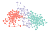 |
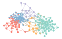 |
| (a) , | (b) , | (c) , | (d) , |
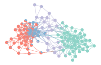 |
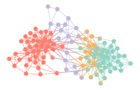 |
\begin{overpic}[width=216.81pt,trim=56.9055pt 34.14322pt 14.22636pt 91.04872pt,clip]{embeding-datapolbooks-multigraphNone-nestedFalse-alt.pdf} \put(48.1,34.1){\color[rgb]{1,0,0}\definecolor[named]{pgfstrokecolor}{rgb}{1,0,0}$\bigstar$} \put(66.6,66.4){\color[rgb]{1,0,0}\definecolor[named]{pgfstrokecolor}{rgb}{1,0,0}$\blacklozenge$} \put(59.0,35.5){\color[rgb]{1,0,0}\definecolor[named]{pgfstrokecolor}{rgb}{1,0,0}$\blacktriangle$} \end{overpic} | |
| (e) , | (f) , | ||
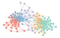 |
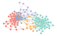 |
||
| (g) , | (h) , | ||
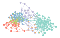 |
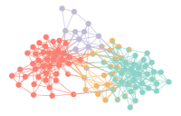 |
||
| (i) , | (j) , | ||
In the following, we consider a simple example that illustrates how the method above can characterize the structure of a distribution of partitions, and we proceed to investigate how the multimodal nature of the posterior distribution can be used to assess the quality of fit of the network model being used.
V.1 Simple example
 |
 |
 |
|---|---|---|
| (a) | (b) | |
 |
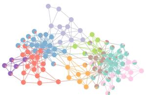 |
|
| (c) | (d) |
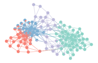
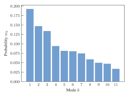
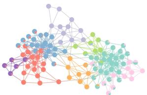
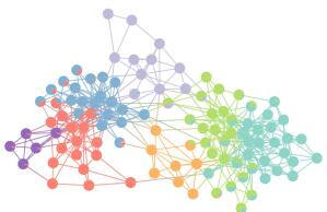
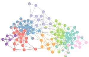
In Fig. 8 we show the result of the above algorithm for the posterior distribution obtained for the same political books network considered previously, where in total modes are identified. For each mode we show the corresponding marginal distribution of the relabeled partitions, and the uncertainty of its maximum , which serves as a quantification of how broadly distributed are the individual modes. As a means of illustration, in Fig. 8 we show also a two-dimensional projection of the distribution of partitions, obtained using the UMAP dimensionality reduction algorithm McInnes et al. (2018) using the maximum overlap distance as the dissimilarity metric (similar results can also be found with other dissimilarity functions, as shown in Appendix D). This algorithm attempts to project the distribution of partitions in two dimensions, while preserving the relative distances between partitions in the projection. As a result we see that each mode is clearly discernible as a local concentration of partitions, much like we would expect of a heterogeneous mixture of continuous variables. We note here that we have not informed the UMAP algorithm of the modes we have found with the algorithm above, and therefore this serves an additional evidence for the existence of the uncovered heterogeneity in the posterior distribution. The most important result of this analysis is that no single mode has a dominating fraction of the distribution, with the largest mode corresponding only to around of the posterior distribution, and with the second largest mode being very close to it. This means that there is no single cohesive picture that emerges from the distribution, and therefore our attempt at summarizing it with a single partition seems particularly ill-suited.
In view of this more detailed picture of the ensemble of partitions, it is worth revisiting the consensus results obtained previously with the various error functions. As shown in Fig. 8, the MAP/VI estimates correspond to the most likely partition of mode (c), which is overall only the third most plausible mode with . From the point of view of the MAP estimator, this serves to illustrate how choosing the most likely partition may in fact run counter to intuition: Although the single most likely partition belongs to mode (c), collectively, the partitions in mode (a) and (b) have a larger plausibility. This means that, if we are forced to choose a single explanation for the data, it would make more sense instead to choose mode (a), despite the fact that it does not contain the single most likely partition. More concretely, when comparing modes (a), (b), and (c), we see that the network does in fact contain more evidence for a division of either the “neutral” or the “liberal” groups into subgroups than the MAP estimate implies, however not both, as mode (d), corresponding to the simultaneous subdivisions, has a smaller plausibility than the other options. The VI estimate also points to mode (c), but it is unclear why. This is indeed a problem with using VI, since despite its strong formal properties, it lacks a clear interpretability.
Differently from MAP and VI, the MOC estimation combines the properties of all modes into a “Frankenstein’s monster,” where local portions of the final inferred partition correspond to different modes. As a result, the resulting point estimate has a very low posterior probability, and hence is a misleading representation of the population — a classic estimation failure of multimodal distributions.
The RMI estimate behaves differently, and corresponds to a typical partition of mode (d), which has an overall plausibility of . We can understand this choice by inspecting its composition, and noticing that the more plausible modes (a) to (c) correspond to partitions where groups of (d) are merged together. Because of this, the RMI similarity sees this partition as the “center” composed of the building blocks required to obtain the other ones via simple operations. But by no means it is the most likely explanation of the data according to the model, and given that it is a division into a larger number of groups, it is more likely to be an overfit, in view of the existence of simpler modes (a) to (c).
V.2 Evaluating model consistency
 |
 |
 |
|---|---|---|
| (a) | (b) |
The full characterization of the posterior distribution with our approach gives us the opportunity to assess the quality of fit between model and data. Indeed, if the model was an excellent fit, e.g. if the data were in fact generated by the SBM, we should expect a single mode in the posterior distribution that is centered in the true partition Decelle et al. (2011) (although the broadness of the mode, represented by the variance of the marginal distribution on the nodes, will depend on how easily detectable the true partition is). Therefore, the fact alone we observe multiple modes is an indication of some degree of mismatch, with the model offering multiple explanations for the data. Since our analysis allows us to inspect each individual explanation, and ascribe to it a plausibility, this can be used to make a more precise evaluation of the fit.
Inspecting the modes observed for the political books network in Fig. 8, we notice that the four largest modes amount approximately to different combinations of the same five groups that appear in the fourth mode (Fig. 8d) — although the remaining modes deviate from this pattern. This is reminiscent of a situation considered by Riolo and Newman Riolo and Newman (2020), who have applied RMI estimation for artificial networks where none of the posterior samples matches the true division, which is only uncovered by the RMI consensus. In particular, in their scenario, the consensus exposed “building blocks,” i.e. groups of nodes that tend to be clustered together, although the building blocks themselves always appear merged together into bigger groups. The situation where the partitions exhibit clear shared building blocks that always appear merged together, but in different combinations, begs the question as to why does the posterior distribution fail to concentrate on the isolated building blocks in the first place. One possibility is that the building blocks do not correspond to the same kind of communities that the inference approach is trying to uncover, e.g. in the case of the SBM these should be nodes that have the same probability of connection to the rest of the network. This would be a case of model mismatch, and hence it would be difficult to interpret what the building blocks actually mean. Another option, that we can address more directly, is that the model being used underfits the data, i.e. the model formulation fails to recognize the available statistical evidence, resulting in the choice of simpler SBMs with fewer groups, such that some “true” groups are merged together. A common cause of underfitting is the use noninformative priors which overly penalize larger numbers of groups, as was shown in Ref. Peixoto (2013). The use of hierarchical priors solves this particular underfitting problem, as discussed in Refs. Peixoto (2014c, 2017). Another potential cause for underfitting is the use of Poisson formulations for the SBM for networks with heterogeneous density, which assumes that the observed simple graph is a possible realization of a multigraph model that generates simple graphs with a very small probability. Ref. Peixoto (2020b) introduced an alternative SBM variation based on a simple but consequential modification of the Poisson SBMs, where multigraphs are generated at a first stage, and the multiedges are converted into simple edges, resulting in a Bernoulli distribution obtained from the cumulative Poisson distribution. These “latent Poisson” SBMs also prevent underfitting, and in fact make the posterior distribution concentrate on the correct answer for the examples considered by Riolo and Newman Riolo and Newman (2020), as shown in Ref. Peixoto (2020b).
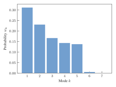
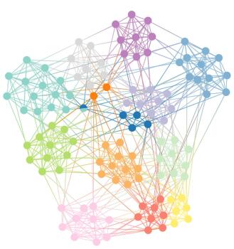
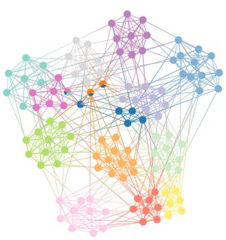
In Fig. 9 we show our method employed on the posterior distribution of the political books network using the latent Poisson DC-SBM with nested priors, which should be able to correct the kinds of underfitting mentioned above. Indeed, the most likely mode shows a more elaborate division of the network into groups, corresponding to particular subdivisions of the same liberal-neutral-conservative groups seen previously. However, these subdivisions are not quite the same as those seen in Fig. 8 for the Poisson SBM. Therefore, in this example it would be futile to search for these uncovered groups in the posterior distribution of the Poisson DC-SBM, even if we search for overlaps between partitions. However, despite the more detailed division of the network, the latent Poisson SBM is far from being a perfect fit for this network, as we still observe modes, corresponding mostly to different divisions of the “conservative” books. When comparing the structure of the different modes, we see that these are not simple combinations of the same subdivisions, but rather different rearrangements. This seems to point to a kind of structure in the network that is not fully captured by the strict division of the nodes in discrete categories, at least not in the manner assumed by the SBM.
In Fig. 10 we compare also the inferences obtained with both SBM models for the karate club network considered previously. The posterior distribution obtained with the Poisson DC-SBM is very heterogeneous, with modes. It has as most plausible mode one composed of a single partition into a single group (implying that the degree sequence alone is enough to explain the network, and no community structure is needed). The second most likely mode corresponds to leader-follower partitions, largely dividing the nodes according to degree (despite the degree correction). The putative division of this network into two assortative communities comes only as the ninth most likely mode. With such an extreme heterogeneity between partitions, finding a consensus between them seems particularly futile, thus explaining the obtained point estimates in Fig. 7, in particular the odd behavior of the RMI estimate that tries to assemble all diverging modes into a single partition. On the other hand, with the latent Poisson SBM the posterior distribution changes drastically, as is shown in right panel of Fig. 10. In this case the dominating mode corresponds to partitions that, while not fully identical to the accepted division, are more compatible with it, as they only further divide one of the communities into two extra groups. The commonly accepted division itself comes as a typical partition of the second most likely mode. Overall, the posterior distribution becomes more homogeneous, with only modes identified, and with most of the posterior probability assigned to the first few.
It is important to observe that the heterogeneity of the posterior distribution by itself cannot be used as a criterion in the decision of which model is a better fit. Indeed, a typical behavior encountered in statistical inference is the “bias-variance trade-off” Geman et al. (1992), where a more accurate representation of the data comes at the cost of increased variance in the set of answers. We illustrate this with a network of American football games Girvan and Newman (2002) shown in Fig. 11. The Poisson DC-SBM yields a very simple posterior distribution, strongly concentrated on a typical partition into groups. On the other hand, as seen in Fig. 12, the latent Poisson DC-SBM yields a more heterogeneous posterior distribution with modes, typically uncovering a larger number of groups. It would be wrong to conclude that the Poisson SBM provides a better fit only because it concentrates on a single answer, if that single answer happens to be underfitting. But from this analysis alone, it is not possible to say if the latent Poisson SBM is not overfitting either. To make the final decision, we need compute the total evidence for each model, as we will consider in Sec. VII. This computation takes the heterogeneity of the posterior distribution into consideration, but combined with the model plausibility.
Before we proceed with model selection, we first show how the methods constructed so far can be generalized for hierarchical partitions, which form the basis of generically better-fitting models of community structure in networks Peixoto (2017).
VI Hierarchical partitions
 |
 |
 |
 |
|---|---|---|---|
| (a) | (b) | (c) |
An important extension of SBM formulations is one where the choice of priors is replaced by a nested sequence of priors and hyperpriors, where groups of nodes are also clustered in their own meta-groups, associated with a coarse-grained version of the network described via its own smaller SBM, and so on recursively, resulting in a nested version of the model Peixoto (2014c, 2017). This hierarchical formulation recovers the usual SBMs when the hierarchy has only a single level, and also introduces many useful properties, including a dramatically reduced tendency to underfit large networks Peixoto (2014c, 2017) as well a simultaneous description of the network structure at several scales of resolution. This model variant takes as parameters a hierarchical partition , where is the group membership of node in level , and each group label in level is a node in the above level , which results in the number of nodes in level being the number of groups in the level below, , except for the first level, . For this model, we have a posterior distribution over hierarchical partitions given by
| (60) |
Like in the non-hierarchical case, this posterior distribution is invariant to label permutations, i.e.
| (61) |
if and are identical up a relabelling of the groups. However in the hierarchical scenario the group relabellings that keep the posterior distribution invariant must keep the same partitions when projected at the lower levels. In other words, the invariant permutation of the labels in level affects the nodes in level . More specifically, if we consider a bijection for labels at level , such that , then we must change the membership in level to . If two hierarchical partitions and are identical up to this kind of transformation, we denote this with the indicator function
| (62) |
or otherwise. Based on this, we can generalize the random label model considered before to model hierarchical partitions sampled from the posterior distribution. We first assume that the labels at all levels are sampled independently as
| (63) |
with
| (64) |
where is the probability that node in level belongs to group . After sampling a partition , we then obtain a final partition by choosing uniformly among all label permutations, yielding
| (65) |
where
| (66) |
If we now consider sampled hierarchical partitions , the posterior distribution of the hidden relabelled hierarchical partitions is given by
| (67) |
where is how often node in level has group label in all samples. Similarly to before, if we consider the conditional probability of a single partition relabelling , but marginalized over the upper levels , we obtain
| (68) |
where are the label counts excluding . Just like in the non-hierarchical case, we can write
| (69) |
up to an unimportant additive constant, where
| (70) |
and is the bijection that matches the groups labels between and . Therefore we can find the maximum of Eq. 69 once more by solving the maximum weight bipartite matching problem with weights given by . This leads to an overall algorithm entirely analogous to the non-hierarchical case, where, starting from some configuration, we remove a sample from the ensemble, and add it again, choosing its labels according to the maximization of Eq. 69, starting from level and going up until , and stopping if such moves no longer increase the posterior probability. Doing a relabel for every sample once takes time , where and are the typical number of nodes and groups at level . Typically, the number of groups decreases exponentially with the hierarchical level, with , so that we have , and thus , the entire running time for a single “sweep” over all samples is then simply , where is the number of labels in the first hierarchical level.
The mixed random label model of Sec. V can also be generalized in a straightforward manner for hierarchical partitions, i.e.
| (71) |
where inside a mode the partitions are sampled according to the hierarchical random label model given by Eq. 65. The inference algorithm from this point onward is exactly the same as in the non-hierarchical case, where we need only to relabel the hierarchical partitions according to Eq. 69 when we move them between modes.
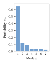
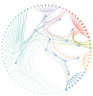
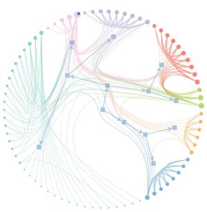
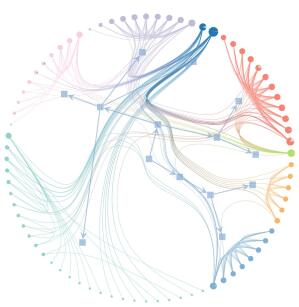
In Fig. 13 we show the inferred modes for hierarchical partitions sampled from the posterior distribution using the nested latent Poisson DC-SBM for a co-occurrence network of characters of the Les Misérables novel Knuth (1993). As this example shows, this algorithm allows us to summarize a multimodal distribution of hierarchical partitions in a rather compact manner. In this particular example we see that the distribution is fairly dominated by one of the modes (shown in Fig. 13a), followed by less probable alternatives.
VI.0.1 Comparing and finding consensus between hierarchical partitions
If we infer the hierarchical random label model above for two hierarchical partitions and , it amounts to solving a recursive maximum bipartite weighted matching problem on every level, starting from to , using as weights the contingency table at each level ,
| (72) |
where is the set of nodes in partition (as upper level partitions might have a disjoint set of nodes), and propagating the matched labels to the upper levels. This is equivalent to maximizing the recursive overlap across all levels
| (73) |
where at each level we need to incorporate the relabeling at the lower levels via
| (74) |
where is a label bijection at level , with the boundary condition . This leads us to the hierarchical maximum overlap distance, defined as
| (75) |
where . A version of this distance that is normalized in the range can be obtained by dividing it by the largest possible value,
| (76) |
It is important to note here that hierarchy levels with a single node, , always have a contribution of zero to the distance, therefore this measure can be applied to infinite hierarchies with , as long as any level is eventually grouped into a single group. For hierarchies with a single level, , we recover the maximum overlap distance considered previously, except for the normalized version, which is slightly different with . This is also a valid normalization for the non-hierarchical distance, since we must always have . The label matching at level of the hierarchy can be done in time , using the sparse version of the Kuhn–Munkres algorithm Kuhn (1955); Munkres (1957); Ramshaw and Tarjan (2012), where is the the number of nonzero entries in the contingency matrix . If we assume once more the typical case with and , so that , the overall computation can then be done in time .
Following the same steps as before, we can use the hierarchical maximum overlap distance as an error function to define a MOC estimator over hierarchical partitions based on the minimization of the mean posterior loss,
| (77) |
Substituting its definition leads us to a set of self-consistent equations at each level ,
| (78) |
with the marginal distributions obtained over the relabeled partitions,
| (79) |
where the relabeling is done in order to maximize the overlap with ,
| (80) |
and where once again we need to recursively incorporate the relabellings at the lower levels,
| (81) |
We can define an uncertainty for this estimator by inspecting the marginal distributions computed along the way,
| (82) |
In the above sum, we omit levels with since those always have a trivial marginal distribution concentrated on a single group. In practice we implement this estimator by sampling a set of hierarchical partitions from the posterior distribution and then performing the sequential maximizations starting from to ,
| (83) | ||||
| (84) |
where is the contingency table of level of sample with . The final solution is obtained when repeating the above maximization no longer changes the result. Like in the non-hierarchical case, this algorithm yields a local optimum of the optimization problem, but not necessarily a global one, therefore it needs to be repeated multiple times with different initial conditions, and the best result kept. Since it involves the relabelling over all hierarchical partitions, the overall algorithmic complexity of a single iteration is , assuming once more the typical case with and .
VII Model selection and evidence approximation
| Data | Poisson | Latent Poisson | Single partition | |||||||||
|---|---|---|---|---|---|---|---|---|---|---|---|---|
| Non-nested | Nested | Non-nested | Nested | Non-nested | Nested | |||||||
| NDC | DC | NDC | DC | NDC | DC | NDC | DC | NDC | DC | NDC | DC | |
| Karate club Zachary (1977) | ||||||||||||
| Dolphins Lusseau et al. (2003) | ||||||||||||
| Les Misérables Knuth (1993) | ||||||||||||
| Political books Krebs | ||||||||||||
| American football Girvan and Newman (2002) | ||||||||||||
| Network scientist Newman (2006) | ||||||||||||
| High school Harris et al. (2009) | ||||||||||||
| C. elegans neurons White et al. (1986) | ||||||||||||
| E-mail Guimerà et al. (2003) | ||||||||||||
| Political blogs Adamic and Glance (2005) | ||||||||||||
If we are interested in comparing two models and in their plausibility for generating some network , we can do so by computing the ratio of their posterior probability given the data,
| (85) |
Therefore, if we are a priori agnostic about either model with , this ratio will be determined by the total probability of the data according to that model. This quantity is called the evidence, and appears as a normalization constant in the posterior distribution of Eq. 1. For any particular choice of model, it is obtained by summing the joint probability of data and partitions over all possible partitions (we drop the explicit dependence on from now on, to unclutter the expressions),
| (86) |
Unfortunately, the exact computation of this sum is intractable since the number of partitions is too large in most cases of interest. It also cannot be obtained directly from samples of the posterior distribution, which makes its estimation from MCMC also very challenging. To illustrate this, it is useful to write the logarithm of the evidence in the following manner,
| (87) | ||||
| (88) |
where
| (89) |
is the posterior distribution of Eq. 1, and
| (90) |
is the mean joint log-probability computed over the posterior distribution, and finally
| (91) |
is the entropy of the posterior distribution. Eq. 87 has the shape of a negative Gibbs free energy of a physical ensemble, if we interpret as the mean negative “energy” over the ensemble of partitions. It tells us that what contributes to the evidence is not only the mean joint probability, but also the multiplicity of solutions with similar probabilities, which is captured by the posterior entropy. In this formulation, we see that while it is possible to estimate from MCMC simply be averaging for sufficiently many samples, the same approach does not work for the entropy term , since it would require the computation of the log-posterior for every sample, something that cannot be done without knowing the normalization constant , which is what we want to find in the first place. However, the mixed random label model of Sec. V can be used to fit the posterior distribution, allowing us to compute the entropy term via the inferred model, and use and the rich information gained on its structure to perform model selection. Let us recall that the mixed random label model, when inferred from partitions sampled from , amounts to an approximation given by
| (92) |
where determines the mode mixture and
| (93) |
are the independent marginal distributions of mode and finally
| (94) |
is the random relabeling of groups. In most cases we have investigated, the inferred modes tend to be very well separated (otherwise they would get merged together into a larger mode), such that we can assume
| (95) |
This means we can write the entropy as
| (96) |
where
| (97) |
is the entropy of the mode mixture distribution, and
| (98) | ||||
| (99) |
is the entropy of mode and
| (100) | ||||
| (101) |
is the relabelling entropy. Putting it all together we have the following approximation for the evidence according to the mixed random label model,
| (102) |
We can extend this for hierarchical partitions in an entirely analogous way, which leads to
| (103) |
The above quantities are then computed by sampling partitions from the posterior distribution, using them (or a superset thereof) to compute the first two means and , and then fit the mixed random label model, from which the parameters and are obtained, and then computing the remaining terms.
In Table 1 we show the evidence obtained for several SBM variants and datasets, including latent Poisson versions (which require special considerations, see Appendix E). Overall, we find that when considering the Poisson SBMs, degree correction is only favored for larger networks, corroborating a similar previous analysis based on a less accurate calculation Peixoto (2017). This changes for latent Poisson models, where for some networks the balance tips in favor of degree correction. Overall, we find more evidence for the latent Poisson models for all networks considered, which is unsurprising given that they are all simple graphs. Likewise, we always find more evidence for the hierarchical SBMs, which further demonstrate their more flexible nature.
VII.1 Bayesian evidence and the minimum description length (MDL) criterion
In this section we explore briefly some direct connections between Bayesian model selection and the minimum description length (MDL) criterion based on information theory Grünwald (2007). We begin by pointing out the simple fact that the MAP point estimate given by the single most likely partition yields a lower bound for the evidence, i.e.
| (104) |
This means that taking into account the full posterior distribution, rather than only its maximum, almost always can be used to compress the data, as we now show. We can see this by inspecting first the usual “two-part” description length,
| (105) | ||||
| (106) |
which corresponds to amount of information necessary to describe the data if one first describes the partition and then, conditioned on it, the network . Therefore, finding the most likely partition means finding the one that most compresses the network, according to this particular two-part encoding. However, the full posterior distribution gives us a more efficient “one-part” encoding where no explicit description of the partition is necessary. Simply defining the joint distribution means we can compute the marginal probability , which yields directly a description length
| (107) |
According to Eq. 104 we have
| (108) |
which means that considering all possible partitions can only increase the overall compression achievable. In Table 1 we can verify that this holds for all results obtained.
In a slightly more concrete setting, let us consider a transmitter who wants to convey the network to a receiver, who both know the joint distribution . According to the two-part code, the transmitter first sends the partition , for that using bits, and then sends the final network using bits, using in total bits. In practice, this is achieved, for example, by both sender and receiver sharing the same two tables of optimal prefix codes derived from and . On the other hand, using the second one-part code, both transmitter and receiver share only a single table of optimal prefix codes derived directly from the marginal distribution , which means that only bits need to be transmitted. In practice, it will be more difficult to construct the one-part code since it involves marginalizing over a high-dimensional distribution, which is intractable via brute force — although our mixed random label model can be used as a basis of an analytical approximation. However what is important in our model selection context is only that such a code exists, not its computational tractability.
VIII Conclusion
We have shown how the random label model can be used to solve the group identification problem in community detection, allowing us to compute marginal distributions of group membership on the nodes in a unambiguous way. This led us to the notion of maximum overlap distance as a general way of comparing two network partitions, which we then used as a loss function to obtain the consensus of a population of network partitions. By investigating the behavior of different loss functions on artificial and empirical ensembles of heterogeneous partitions, we have demonstrated that they can yield inconsistent results, due precisely to a lack of uniformity between divisions. We then developed a more comprehensive characterization of the posterior distribution, based on a mixed version of the random label model that is capable of describing multimodal populations of partitions, where multiple consensuses exist at the same time. This kind of structure corresponds to a “multiple truths” phenomenon, where a model can yield diverging hypotheses for the same data. We showed how our method provides a compact representation for structured populations of network partitions, and allows us to assess quality of fit and perform model selection. The latter was achieved by using the multimodal fit of the posterior distribution as a proxy for the computation of its entropy, which is a key but often elusive ingredient in Bayesian model selection.
Although we have focused on community detection, the methods developed here are applicable for any kind of clustering problem from which a population of answers can be produced. They allow us to be more detailed in our assessment of the consistency of results when applied to real or artificial data. In particular, we no longer need to rely on “point estimates” that can give a very misleading picture of high dimensional and structured populations of partitions, even if they attempt to assemble a consensus among them. We achieve this without losing interpretability, as our method yields groupings of partitions that share a local consensus, each telling a different version of how the data might have been generated, and weighted according to the statistical evidence available.
References
- Fortunato (2010) Santo Fortunato, “Community detection in graphs,” Physics Reports 486, 75–174 (2010).
- Fortunato and Hric (2016) Santo Fortunato and Darko Hric, “Community detection in networks: A user guide,” Physics Reports (2016), 10.1016/j.physrep.2016.09.002.
- Good et al. (2010) Benjamin H. Good, Yves-Alexandre de Montjoye, and Aaron Clauset, “Performance of modularity maximization in practical contexts,” Physical Review E 81, 046106 (2010).
- Brandes et al. (2006) U. Brandes, D. Delling, M. Gaertler, R. Görke, M. Hoefer, Z. Nikoloski, and D. Wagner, “On modularity-np-completeness and beyond,” ITI Wagner, Faculty of Informatics, Universität Karlsruhe (TH), Tech. Rep 19, 2006 (2006).
- Decelle et al. (2011) Aurelien Decelle, Florent Krzakala, Cristopher Moore, and Lenka Zdeborová, “Asymptotic analysis of the stochastic block model for modular networks and its algorithmic applications,” Physical Review E 84, 066106 (2011).
- Guimerà and Sales-Pardo (2009) Roger Guimerà and Marta Sales-Pardo, “Missing and spurious interactions and the reconstruction of complex networks,” Proceedings of the National Academy of Sciences 106, 22073 –22078 (2009).
- Clauset et al. (2008) Aaron Clauset, Cristopher Moore, and M. E. J. Newman, “Hierarchical structure and the prediction of missing links in networks,” Nature 453, 98–101 (2008).
- Calatayud et al. (2019) Joaquín Calatayud, Rubén Bernardo-Madrid, Magnus Neuman, Alexis Rojas, and Martin Rosvall, “Exploring the solution landscape enables more reliable network community detection,” Physical Review E 100, 052308 (2019), publisher: American Physical Society.
- Riolo and Newman (2020) Maria A. Riolo and M. E. J. Newman, “Consistency of community structure in complex networks,” Physical Review E 101, 052306 (2020), publisher: American Physical Society.
- Strehl and Ghosh (2002) Alexander Strehl and Joydeep Ghosh, “Cluster Ensembles — A Knowledge Reuse Framework for Combining Multiple Partitions,” Journal of Machine Learning Research 3, 583–617 (2002).
- Topchy et al. (2005) A. Topchy, A.K. Jain, and W. Punch, “Clustering ensembles: models of consensus and weak partitions,” IEEE Transactions on Pattern Analysis and Machine Intelligence 27, 1866–1881 (2005), conference Name: IEEE Transactions on Pattern Analysis and Machine Intelligence.
- Goder and Filkov (2008) Andrey Goder and Vladimir Filkov, “Consensus Clustering Algorithms: Comparison and Refinement,” in 2008 Proceedings of the Workshop on Algorithm Engineering and Experiments (ALENEX), Proceedings (Society for Industrial and Applied Mathematics, 2008) pp. 109–117.
- Lancichinetti and Fortunato (2012) Andrea Lancichinetti and Santo Fortunato, “Consensus clustering in complex networks,” Scientific Reports 2, 1–7 (2012), number: 1 Publisher: Nature Publishing Group.
- Zhang and Moore (2014) Pan Zhang and Cristopher Moore, “Scalable detection of statistically significant communities and hierarchies, using message passing for modularity,” Proceedings of the National Academy of Sciences 111, 18144–18149 (2014), publisher: National Academy of Sciences Section: Physical Sciences.
- Tandon et al. (2019) Aditya Tandon, Aiiad Albeshri, Vijey Thayananthan, Wadee Alhalabi, and Santo Fortunato, “Fast consensus clustering in complex networks,” Physical Review E 99, 042301 (2019), publisher: American Physical Society.
- Maaten and Hinton (2008) Laurens van der Maaten and Geoffrey Hinton, “Visualizing Data using t-SNE,” Journal of Machine Learning Research 9, 2579–2605 (2008).
- McInnes et al. (2018) Leland McInnes, John Healy, and James Melville, “UMAP: Uniform Manifold Approximation and Projection for Dimension Reduction,” arXiv:1802.03426 [cs, stat] (2018), arXiv: 1802.03426.
- Peixoto (2019) Tiago P. Peixoto, “Bayesian Stochastic Blockmodeling,” in Advances in Network Clustering and Blockmodeling (John Wiley & Sons, Ltd, 2019) pp. 289–332.
- Holland et al. (1983) Paul W. Holland, Kathryn Blackmond Laskey, and Samuel Leinhardt, “Stochastic blockmodels: First steps,” Social Networks 5, 109–137 (1983).
- Peixoto (2014a) Tiago P. Peixoto, “Efficient Monte Carlo and greedy heuristic for the inference of stochastic block models,” Physical Review E 89, 012804 (2014a).
- Riolo et al. (2017) Maria A. Riolo, George T. Cantwell, Gesine Reinert, and M. E. J. Newman, “Efficient method for estimating the number of communities in a network,” Physical Review E 96, 032310 (2017).
- Peixoto (2020a) Tiago P. Peixoto, “Merge-split Markov chain Monte Carlo for community detection,” arXiv:2003.07070 [physics, stat] (2020a), arXiv: 2003.07070.
- (23) V Krebs, “Political Books Network,” unpublished, retrieved from Mark Newman’s website: http://www-personal.umich.edu/{~}mejn/netdata/ .
- Karrer and Newman (2011) Brian Karrer and M. E. J. Newman, “Stochastic blockmodels and community structure in networks,” Physical Review E 83, 016107 (2011).
- Peixoto (2017) Tiago P. Peixoto, “Nonparametric Bayesian inference of the microcanonical stochastic block model,” Physical Review E 95, 012317 (2017).
- Ramshaw and Tarjan (2012) Lyle Ramshaw and Robert E. Tarjan, “On minimum-cost assignments in unbalanced bipartite graphs,” HP Labs, Palo Alto, CA, USA, Tech. Rep. HPL-2012-40R1 (2012).
- Kuhn (1955) H. W. Kuhn, “The Hungarian method for the assignment problem,” Naval Research Logistics Quarterly 2, 83–97 (1955), publisher: John Wiley & Sons, Ltd.
- Munkres (1957) James Munkres, “Algorithms for the Assignment and Transportation Problems,” Journal of the Society for Industrial and Applied Mathematics 5, 32–38 (1957).
- Peixoto (2014b) Tiago P. Peixoto, “The graph-tool python library,” figshare (2014b), 10.6084/m9.figshare.1164194, available at https://graph-tool.skewed.de.
- Meilă and Heckerman (2001) Marina Meilă and David Heckerman, “An Experimental Comparison of Model-Based Clustering Methods,” Machine Learning 42, 9–29 (2001).
- Meilǎ (2005) Marina Meilǎ, “Comparing clusterings: an axiomatic view,” in Proceedings of the 22nd international conference on Machine learning (2005) pp. 577–584.
- Meilă (2007) Marina Meilă, “Comparing clusterings—an information based distance,” Journal of Multivariate Analysis 98, 873–895 (2007).
- Meilă (2003) Marina Meilă, “Comparing Clusterings by the Variation of Information,” in Learning Theory and Kernel Machines, Lecture Notes in Computer Science No. 2777, edited by Bernhard Schölkopf and Manfred K. Warmuth (Springer Berlin Heidelberg, 2003) pp. 173–187.
- Newman et al. (2020) M. E. J. Newman, George T. Cantwell, and Jean-Gabriel Young, “Improved mutual information measure for clustering, classification, and community detection,” Physical Review E 101, 042304 (2020), publisher: American Physical Society.
- Zachary (1977) Wayne W. Zachary, “An Information Flow Model for Conflict and Fission in Small Groups,” Journal of Anthropological Research 33, 452–473 (1977).
- Peixoto (2013) Tiago P. Peixoto, “Parsimonious Module Inference in Large Networks,” Physical Review Letters 110, 148701 (2013).
- Peixoto (2014c) Tiago P. Peixoto, “Hierarchical Block Structures and High-Resolution Model Selection in Large Networks,” Physical Review X 4, 011047 (2014c).
- Peixoto (2020b) Tiago P. Peixoto, “Latent Poisson models for networks with heterogeneous density,” arXiv:2002.07803 [physics, stat] (2020b), arXiv: 2002.07803.
- Geman et al. (1992) Stuart Geman, Elie Bienenstock, and René Doursat, “Neural Networks and the Bias/Variance Dilemma,” Neural Computation 4, 1–58 (1992), publisher: MIT Press.
- Girvan and Newman (2002) M. Girvan and M. E. J. Newman, “Community structure in social and biological networks,” Proceedings of the National Academy of Sciences 99, 7821 –7826 (2002).
- Knuth (1993) Donald E. Knuth, The Stanford GraphBase: A Platform for Combinatorial Computing, 1st ed. (Addison-Wesley Professional, New York, N.Y. : Reading, Mass, 1993).
- Lusseau et al. (2003) David Lusseau, Karsten Schneider, Oliver J. Boisseau, Patti Haase, Elisabeth Slooten, and Steve M. Dawson, “The bottlenose dolphin community of Doubtful Sound features a large proportion of long-lasting associations,” Behavioral Ecology and Sociobiology 54, 396–405 (2003).
- Newman (2006) M. E. J. Newman, “Finding community structure in networks using the eigenvectors of matrices,” Physical Review E 74, 036104 (2006).
- Harris et al. (2009) Kathleen Mullan Harris, Carolyn T. Halpern, Eric Whitsel, Jon Hussey, Joyce Tabor, Pamela Entzel, and J. Richard Udry, “The national longitudinal study of adolescent to adult health: Research design,” See http://www. cpc. unc. edu/projects/addhealth/design (accessed 9 April 2015) (2009).
- White et al. (1986) J. G. White, E. Southgate, J. N. Thomson, and S. Brenner, “The structure of the nervous system of the nematode Caenorhabditis elegans,” Philosophical Transactions of the Royal Society of London. Series B, Biological Sciences 314, 1–340 (1986).
- Guimerà et al. (2003) R. Guimerà, L. Danon, A. Díaz-Guilera, F. Giralt, and A. Arenas, “Self-similar community structure in a network of human interactions,” Physical Review E 68, 065103 (2003).
- Adamic and Glance (2005) Lada A. Adamic and Natalie Glance, “The political blogosphere and the 2004 U.S. election: divided they blog,” in Proceedings of the 3rd international workshop on Link discovery, LinkKDD ’05 (ACM, New York, NY, USA, 2005) pp. 36–43.
- Grünwald (2007) Peter D. Grünwald, The Minimum Description Length Principle (The MIT Press, 2007).
- Gates et al. (2019) Alexander J. Gates, Ian B. Wood, William P. Hetrick, and Yong-Yeol Ahn, “Element-centric clustering comparison unifies overlaps and hierarchy,” Scientific Reports 9, 1–13 (2019), number: 1 Publisher: Nature Publishing Group.
- Zhang et al. (2016) Pan Zhang, Cristopher Moore, and M. E. J. Newman, “Community detection in networks with unequal groups,” Physical Review E 93, 012303 (2016).
- Rezaei and Fränti (2016) Mohammad Rezaei and Pasi Fränti, “Set Matching Measures for External Cluster Validity,” IEEE Transactions on Knowledge and Data Engineering 28, 2173–2186 (2016), conference Name: IEEE Transactions on Knowledge and Data Engineering.
- Amigó et al. (2009) Enrique Amigó, Julio Gonzalo, Javier Artiles, and Felisa Verdejo, “A comparison of extrinsic clustering evaluation metrics based on formal constraints,” Information Retrieval 12, 461–486 (2009).
- Kunegis (2013) Jérôme Kunegis, “KONECT: The Koblenz Network Collection,” in Proceedings of the 22Nd International Conference on World Wide Web, WWW ’13 Companion (ACM, New York, NY, USA, 2013) pp. 1343–1350.
- Ghasemian et al. (2019) Amir Ghasemian, Homa Hosseinmardi, and Aaron Clauset, “Evaluating Overfit and Underfit in Models of Network Community Structure,” IEEE Transactions on Knowledge and Data Engineering , 1–1 (2019).
Appendix A Properties of the maximum overlap distance
In Sec. III.1 of the main text we considered the maximum overlap distance, which corresponds to the minimal classification error, i.e. the smallest possible number of nodes with an incorrect group placement in a partition if another partition is assumed to be the correct one. It is defined as
| (109) |
This measure has been considered before in Refs. Meilă and Heckerman (2001); Meilǎ (2005); Meilă (2007), and here we review some of its useful properties.
-
1.
Simple interpretation. Since it quantifies the classification error, it is easy to intuitively understand what the distance is conveying. In particular its normalized version yields values in the range which can be interpreted as fractions of differing nodes, and hence allows the direct comparison between results obtained for partitions of different sizes and numbers of groups.
-
2.
Behaves well for unbalanced partitions. The distance behaves as one would expect even when the partitions have very different number of groups, or the number of groups approaches for either or , unlike alternatives such as mutual information Gates et al. (2019). More specifically, if we simply increase the number of groups of either partition being compared, this does not spuriously introduce small values of . We see this by noticing that if and , the maximum overlap is always , since each group in can be trivially matched with any of the single-node groups in , yielding
(110) which leads to the maximum normalized distance as .
-
3.
Simple asymptotic behavior for uncorrelated partitions. Suppose partitions and are sampled independently and uniformly from the set of all possible partitions into and labelled groups, respectively. In this case, as , the contingency table will tend to the uniform one with , which results in the asymptotic normalized distance given by
(111) Although it is not a substitute for a proper hypothesis test (which would need to account for finite values of ), this asymptotic value gives a rule of thumb of how to interpret the distance between two partitions as a strength of statistical correlation.
-
4.
Defines a metric space. The distance is a proper metric, since it fulfills the properties of identity , non-negativity , symmetry , and most notably, triangle inequality (we offer a simple proof of this in Appendix B). This makes this notion of distance well-defined, unambiguous, and conforming to intuition.
-
5.
Information-theoretic interpretation. The maximum overlap has a direct information theoretic interpretation, due to its connection to the random label generative model exposed earlier. According to the model of Eq. 12 the joint probability of observing two partitions , up to an arbitrary relabelling of the groups, is given by
(112) This means that any two partitions have a joint description length
(113) (114) which measures the amount of information (in bits) necessary to describe both partitions. The above quantity is proportional to the negative value of the maximum overlap , and hence is proportional to . (Note that this is not the most efficient encoding scheme based on the maximum overlap, we consider an alternative in Appendix C.)
-
6.
Efficient computation. As discussed previously, computing the maximum overlap involves solving an instance of the maximum bipartite weighted matching problem, with weights given by the contingency table, (see Fig. 2), which can be done using the Kuhn–Munkres algorithm Kuhn (1955); Munkres (1957). In its sparse version, the running time is bound by , with being the number of nonzero entries in the contingency matrix Ramshaw and Tarjan (2012). Combining this with the work required to build the contingency table itself, the computation of is bound by . Therefore the running time will depend on whether we expect the number of labels and the density of the contingency table to be much smaller or comparable to . In the former case, the maximum matching algorithm takes a comparatively negligible time, and the linear term dominates, yielding a running time . Otherwise, if we have or , then , and hence the running time will be quadratic, . However, the latter scenario is atypical when is very large, so therefore we most often encounter the linear regime allowing for very fast computations (see Fig. 14).
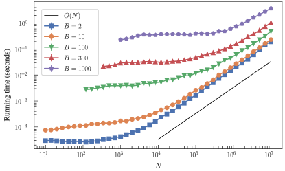
The maximum overlap distance has been used before in situations where the labeling is unambiguous or the number of labels is so small that exhaustive iteration over label permutations is feasible (e.g. Decelle et al. (2011); Zhang et al. (2016)), but, to the best of our knowledge, rarely in combination with the maximum bipartite weighted matching algorithm as outlined above (with an exception being Ref. Rezaei and Fränti (2016) that employed it when comparing with other metrics) which makes it usable in general settings. Instead, more focus has been given to measures such as mutual information (and its several variants) Amigó et al. (2009) or variation of information (VI) Meilă (2003), which are based on the contingency table without requiring us to obtain a label matching. As pointed out by Meilă Meilă (2003), it is not meaningful to talk about the “best” way of comparing partitions without any context, since such a task must be unavoidably tied with our ultimate objective. Therefore, a different set of axiomatic conditions might prefer another dissimilarity function, and indeed it can be proven that no single function can simultaneously fulfil some elementary set of axioms Meilǎ (2005). In particular, since the maximum overlap distance is based only on the number of nodes correctly classified, it ignores the nodes that do not match, and hence does not exploit any potential regularity with which the labels are mismatched. Other functions such as variation of information, might provide alternatives which can be used to highlight different properties of partition ensembles. Nevertheless, few other dissimilarity functions share the same ease of interpretation with the maximum overlap distance, while possessing its other useful formal properties, such as natural normalization, information-theoretical interpretation, and the fact it defines a metric space.
Among the alternative partition similarities and dissimilarities, the recently introduced reduced mutual information (RMI) Newman et al. (2020) deserves particular mention. This is because, like the maximum overlap distance, it is related to a joint description length of two partitions, which in the case of RMI involves encoding the full contingency table. This means that both similarities can be compared to each other in their own terms, and the most appropriate measure must yield the shortest description length. We perform a succinct comparison between RMI and an overlap-based encoding in Appendix C. We will also consider both RMI and VI more closely in the following section.
Appendix B Maximum overlap distance obeys triangle inequality
Here we show that the maximum overlap distance of Eq. 26 obeys triangle inequality, i.e.
| (115) |
for any set of labelled partitions , , and . Let us consider the maximum overlap
| (116) |
Now for an arbitrary choice of , and let us consider the sum
| (117) |
The maximum value either term in the above sum can take is , corresponding to partitions that are identical up to relabeling, i.e. or . If we condition on one of the terms taking its maximum value , the remaining term can take a value at most , either via the first term with if or via the second term with with . This means we can write
| (118) |
Substituting and rearranging gives us Eq. 115.
Appendix C Encoding partitions based on overlap
As described in the main text, the random label model yields a description length for a pair of partitions given by
| (119) | ||||
| (120) |
Likewise, if we observe , and use to describe partition , the additional amount of information we need to convey is
| (121) | ||||
| (122) | ||||
| (123) |
where we have used from Eq. 12. From this we can note that this encoding is sub-optimal in the sense that even when the overlapping is maximal with , the additional information needed to encode is which is scales as when .
Nevertheless we can develop a different encoding that is more efficient at using the overlap information. We do so by incorporating it as an explicit parameter as follows:
-
1.
We sample an overlap value uniformly in the range , such that
(124) -
2.
We chose a subset of the nodes of size , uniformly with probability
(125) -
3.
For the nodes in we sample a partition with probability
(126) which leads to a marginal distribution
(127) (128) where , assuming a uniform prior .
-
4.
For the remaining nodes not in we sample the values of partitions and analogously, i.e.
with and .
-
5.
For the nodes we set , and we choose a label bijection uniformly at random from the set of size and use to relabel either or arbitrarily.
In the end, this model generates partitions and that have an overlap at least , although the actual overlap can be larger by chance. The scheme above allows groups to be unpopulated in the final partition, which is sub-optimal, but this can be neglected for our current purpose. The final joint probability of this scheme is
| (129) |
which leads to a description length
| (130) |
The minimum description length for and is given by
| (131) |
which corresponds simply to finding the maximum overlap and the corresponding label matching between and from which , and can be derived. It is easy to see now that if the overlap is maximal with , the description length amounts to
| (132) |
where we have chosen as the reference partition arbitrarily, but without loss of generality. Hence, if we subtract the necessary information required to describe , given by
| (133) |
we are left with negligible logarithmic terms
| (134) |
meaning the additional information needed to describe given is vanishingly small with respect to , and hence the code is efficient in this case.
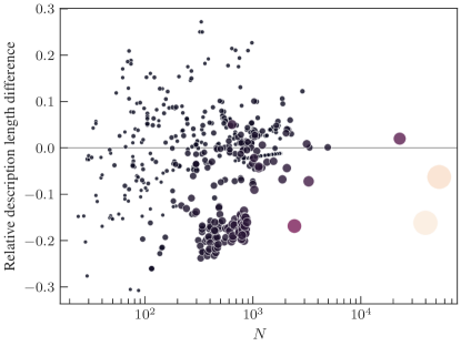 |
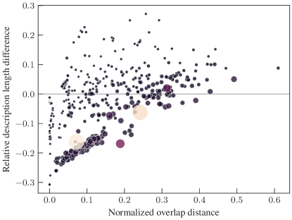 |
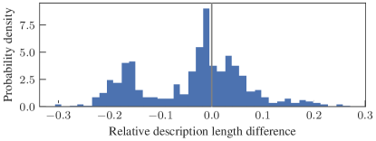 |
It is instructive to compare the above scheme with the reduced mutual information (RMI) encoding recently proposed in Ref. Newman et al. (2020). It corresponds to a three part scheme where one encodes first partition , then the full contingency table between both partitions , and finally the remaining partition , leading to a description length
| (135) |
where and are the number of labels in partitions and and is the number of possible contingency tables with row and column sums given by and , which cannot be computed in closed form, but for which approximations are available (see Ref. Newman et al. (2020)). Note that the encoding above is not symmetric, i.e. in general , as the overall description length will depend on which partition is encoded first (although the relative description length is always symmetric). Therefore the minimum description length amounts to choosing the optimal partition to encode first
| (136) |
In Fig. 15 we compare the compression of two partitions sampled independently from the DC-SBM posterior distribution of 571 empirical networks selected from the Konect Kunegis (2013) and CommunityFitNet Ghasemian et al. (2019) repositories. Overall, we observe somewhat mixed results with, the overlap encoding providing a better compression for around of the networks. As we might expect, the overlap encoding tends to provide a better description if the overlap between partitions is very high, such that a full description of the non-matching nodes becomes superfluous. Otherwise, for highly differing partitions, the RMI encoding is able to capture similarities more efficiently.
Appendix D Comparison with dimensionality reduction
The clustering algorithm presented in Sec. V of the main text is based on a particular definition of what a mode is, according to the random label model presented in Sec. III. As has been shown in Fig. 9, there is an intimate relationship between the clusters founds and the metric space of partitions as defined by the maximum overlap distance, such that dimensionality reduction algorithms like UMAP tend to identify the same clusters. One may wonder, however, if this picture changes if we consider another underlying metric space defined by a different distance function. To give a glimpse into this question, in Fig. 16 are shown the results of dimensionality reduction using both the variation and information and reduced mutual information222The reduced mutual information is not a metric distance, since it does not obey triangle inequality, hence it is not really suitable for use with UMAP, which requires a true metric. Nevertheless, the results obtained are robust even to this inconsistency. functions, both of which make use of the entire contingency table when comparing partitions.
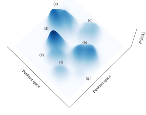 |
| (a) Variation of information (VI) |
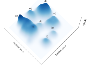 |
| (b) Reduced mutual information (RMI) |
As we can see, not only the overall the multimodal structure is preserved, but also the composition of the modes is compatible with was obtained in Fig. 9, showing that the existence of the clusters is not intrinsically tied with the modelling choices made, but are in fact a property of the data that can be probed in different ways. Naturally, the local shapes and relative positions of the modes vary according to the distance used — and in fact even across different runs of the UMAP algorithm, since it is nondeterministic.
We stress that the approach we present in the main text offers many advantages over dimensionality reduction, namely: 1. We know from the beginning what the identified modes mean, and is not something that needs to be interpreted a posteriori; 2. Clustering is performed in a nonparametric manner, without having to decide on an embedding dimension, or even the number of clusters that need to be found. Dimensionality reduction, on the other hand, comprises only an intermediary step that yields an input to a surrogate clustering algorithm, like k-means, which is often parametric.
Appendix E Evidence for latent Poisson SBMs
The latent Poisson SBMs of Ref. Peixoto (2020b) are generative models for simple graphs, where at first a multigraph is generated with probability
| (137) |
from a Poisson SBM, and then a simple graph is obtained by collapsing the multiedges to simple edges with
| (138) |
The joint posterior distribution of partitions and latent multiedges is then
| (139) |
with evidence given by
| (140) |
Because of the latent multiedges, we need to approximate the evidence in a similar, but different manner. We write the log evidence as
| (141) | ||||
| (142) |
where
| (143) |
is the joint posterior distribution. For our approximation we assume the factorization,
| (144) |
together with the “mean-field” over the latent multiedges,
| (145) |
with the marginals estimated via MCMC
| (146) |
so that the latent edge entropy can be computed as
| (147) |
From this we obtain the final approximation,
| (148) |
where is computed using the mixed random label models as done in the main text. The approximation for the hierarchical model follows analogously.