Boundary-free Kernel-smoothed Goodness-of-fit Tests for Data on General Interval

[Uncaptioned image] Rizky Reza Fauzi
Graduate School of Mathematics
Kyushu University
744 Motooka, Nishi-ku, Fukuoka-shi, Fukuoka-ken, JAPAN
fauzi.rizky.853@s.kyushu-u.ac.jp
&Yoshihiko Maesono
Faculty of Sciemce and Engineering
Chuo University
1-13-27 Kasuga, Bunkyo-ku, Tokyo-to, JAPAN
maesono@math.chuo-u.ac.jp
corresponding author
Abstract

We propose kernel-type smoothed Kolmogorov-Smirnov and Cramér-von Mises tests for data on general interval, using bijective transformations. Though not as severe as in the kernel density estimation, utilizing naive kernel method directly to those particular tests will result in boundary problem as well. This happens mostly because the value of the naive kernel distribution function estimator is still larger than 00 (or less than 111) when it is evaluated at the boundary points. This situation can increase the errors of the tests especially the second-type error. In this article, we use bijective transformations to eliminate the boundary problem. Some simulation results illustrating the estimator and the tests’ performances will be presented in the last part of this article.

Keywords Bijective function  \cdot Cramér-von Mises test  \cdot Distribution function  \cdot Goodness-of-fit test  \cdot Kernel smoothing  \cdot Kolmogorov-Smirnov test  \cdot Transformation

1 Introduction

Many statistical methods depend on an assumption that the data under consideration are drawn from a certain distribution, or at least from a distribution that is approximately similar to that particular distribution. For example, test of normality for residuals are needed after fitting a linear regression in order to satisfy the normality assumption of the model. Distributional assumption is important because, in most cases, it dictates the methods that can be used to estimate the unknown parameters and also determines the procedures that staticticians may apply. There are some goodness-of-fit tests available to determine whether a sample comes from the assumed distribution. Those popular tests include the Kolmogorov-Smirnov (KS) test, Cramér-von Mises (CvM) test, Anderson-Darling test, and Durbin-Watson test. In this article, we will be focusing ourselves to the KS and CvM tests.

Let X1,X2,,Xnsubscript𝑋1subscript𝑋2subscript𝑋𝑛X_{1},X_{2},...,X_{n} be independently and identically distributed random variables supported on ΩΩ\Omega\subseteq\mathbb{R} with an absolutely continuous distribution function FXsubscript𝐹𝑋F_{X} and a density fXsubscript𝑓𝑋f_{X}. The classical nonparametric estimator of FXsubscript𝐹𝑋F_{X} has been the empirical distribution function defined by

Fn(x)=1ni=1nI(Xix),x,formulae-sequencesubscript𝐹𝑛𝑥1𝑛superscriptsubscript𝑖1𝑛𝐼subscript𝑋𝑖𝑥𝑥\displaystyle F_{n}(x)=\frac{1}{n}\sum_{i=1}^{n}I(X_{i}\leq x),\;\;\;x\in\mathbb{R}, (1)

where I(A)𝐼𝐴I(A) denotes the indicator function of a set A𝐴A. It is obvious that Fnsubscript𝐹𝑛F_{n} is a step function of height 1n1𝑛\frac{1}{n} at each observed sample point Xi=xisubscript𝑋𝑖subscript𝑥𝑖X_{i}=x_{i}. When considered as a pointwise estimator of FX(x)subscript𝐹𝑋𝑥F_{X}(x), Fn(x)subscript𝐹𝑛𝑥F_{n}(x) is an unbiased and strongly consistent estimator with Var[Fn(x)]=n1FX(x)[1FX(x)]𝑉𝑎𝑟delimited-[]subscript𝐹𝑛𝑥superscript𝑛1subscript𝐹𝑋𝑥delimited-[]1subscript𝐹𝑋𝑥Var[F_{n}(x)]=n^{-1}F_{X}(x)[1-F_{X}(x)].

In this setting, the Kolmogorov-Smirnov statistic utilizes the empirical distribution function Fnsubscript𝐹𝑛F_{n} to test the null hypothesis

H0:FX=F:subscript𝐻0subscript𝐹𝑋𝐹\displaystyle H_{0}:F_{X}=F

againsts the alternative hypothesis

H1:FXF,:subscript𝐻1subscript𝐹𝑋𝐹\displaystyle H_{1}:F_{X}\neq F,

where F𝐹F is the assumed distribution function. The test statistic is defined as

KSn=supx|Fn(x)F(x)|.𝐾subscript𝑆𝑛subscriptsupremum𝑥subscript𝐹𝑛𝑥𝐹𝑥\displaystyle KS_{n}=\sup_{x\in\mathbb{R}}|F_{n}(x)-F(x)|. (2)

If under a significance level α𝛼\alpha the value of KSn𝐾subscript𝑆𝑛KS_{n} is larger than a certain value from Kolmogorov distribution table, we will reject H0subscript𝐻0H_{0}. Likewise, under the same circumstance, the statistic of the Cramér-von Mises test is defined as

CvMn=n[Fn(x)F(x)]2dF(x),𝐶𝑣subscript𝑀𝑛𝑛superscriptsubscriptsuperscriptdelimited-[]subscript𝐹𝑛𝑥𝐹𝑥2differential-d𝐹𝑥\displaystyle CvM_{n}=n\int_{-\infty}^{\infty}[F_{n}(x)-F(x)]^{2}\mathrm{d}F(x), (3)

and we reject the null hypothesis when the value of CvMn𝐶𝑣subscript𝑀𝑛CvM_{n} is larger than a certain value from Cramér-von Mises table.

Several discussions regarding those goodness-of-fit tests have been around for decades. The recent articles include the distribution of KS and CvM tests for exponential populations (Evans et al. 2017), revision of two-sample KS test (Finner and Gontscharuk 2018), KS test for mixed distributions (Zierk et al. 2020), KS test for bayesian ensembles of phylogenies (Antoneli et al. 2018), CvM distance for neighbourhood-of-model validation (Baringhaus and Henze 2016), rank-based CvM test (Curry et al. 2019), and model selection using CvM distance in a fixed design regression (Chen et al. 2018).

Though the standard KS and CvM tests work really well, but it does not mean they bear no problem. The lack of smoothness of Fnsubscript𝐹𝑛F_{n} causes too much sensitivity near the center of distribution, especially when n𝑛n is small. Hence, it is not unusual to find the supremum value of |Fn(x)F(x)|subscript𝐹𝑛𝑥𝐹𝑥|F_{n}(x)-F(x)| is attained when x𝑥x is near the center of distribution, or the value of CvMn𝐶𝑣subscript𝑀𝑛CvM_{n} gets larger because [Fn(x)F(x)]2superscriptdelimited-[]subscript𝐹𝑛𝑥𝐹𝑥2[F_{n}(x)-F(x)]^{2} is large when the data is highly concentrated in one area. Furthermore, given the information that FXsubscript𝐹𝑋F_{X} is absolutely continuous, it seems to be more appropriate to use a smooth and continuous estimator of FXsubscript𝐹𝑋F_{X} rather than the empirical distribution function Fnsubscript𝐹𝑛F_{n} for testing the goodness-of-fit.

The other maneuver that can be used for estimating the cummulative distribution function nonparametrically is the kernel method. Let K(x)𝐾𝑥K(x) be a symmetric continuous nonnegative kernel function with K(x)dx=1superscriptsubscript𝐾𝑥differential-d𝑥1\int_{-\infty}^{\infty}K(x)\mathrm{d}x=1, and h>00h>0 be the bandwidth satisfying h00h\rightarrow 0 and nh𝑛nh\rightarrow\infty when n𝑛n\rightarrow\infty. Hence, Nadaraya (1964) defined the naive kernel distribution function estimator as

F^X(x)=1ni=1nW(xXih),x,formulae-sequencesubscript^𝐹𝑋𝑥1𝑛superscriptsubscript𝑖1𝑛𝑊𝑥subscript𝑋𝑖𝑥\displaystyle\widehat{F}_{X}(x)=\frac{1}{n}\sum_{i=1}^{n}W\left(\frac{x-X_{i}}{h}\right),\;\;\;x\in\mathbb{R}, (4)

where W(v)=vK(w)dw𝑊𝑣superscriptsubscript𝑣𝐾𝑤differential-d𝑤W(v)=\int_{-\infty}^{v}K(w)\mathrm{d}w. It is easy to prove that this kernel distribution function estimator is continuous, and satisfies all the properties of a distribution function.

Several properties of F^Xsubscript^𝐹𝑋\widehat{F}_{X} are well known. The bias and the variance are

Bias[F^X(x)]=h22fX(x)v2K(v)dv+o(h2),𝐵𝑖𝑎𝑠delimited-[]subscript^𝐹𝑋𝑥superscript22superscriptsubscript𝑓𝑋𝑥superscriptsubscriptsuperscript𝑣2𝐾𝑣differential-d𝑣𝑜superscript2\displaystyle Bias[\widehat{F}_{X}(x)]=\frac{h^{2}}{2}f_{X}^{\prime}(x)\int_{-\infty}^{\infty}v^{2}K(v)\mathrm{d}v+o(h^{2}), (5)
Var[F^X(x)]=1nFX(x)[1FX(x)]2hnr1fX(x)+o(hn),𝑉𝑎𝑟delimited-[]subscript^𝐹𝑋𝑥1𝑛subscript𝐹𝑋𝑥delimited-[]1subscript𝐹𝑋𝑥2𝑛subscript𝑟1subscript𝑓𝑋𝑥𝑜𝑛\displaystyle Var[\widehat{F}_{X}(x)]=\frac{1}{n}F_{X}(x)[1-F_{X}(x)]-\frac{2h}{n}r_{1}f_{X}(x)+o\left(\frac{h}{n}\right), (6)

where r1=vK(v)W(v)dvsubscript𝑟1superscriptsubscript𝑣𝐾𝑣𝑊𝑣differential-d𝑣r_{1}=\int_{-\infty}^{\infty}vK(v)W(v)\mathrm{d}v. The almost sure uniform convergence of F^Xsubscript^𝐹𝑋\widehat{F}_{X} to FXsubscript𝐹𝑋F_{X} was proved by Nadaraya (1964), Winter (1973), and Yamato (1973), while Yukich (1989) extended this result to higher dimensions. Watson and Leadbetter (1964) proved the asymptotic normality of F^X(x)subscript^𝐹𝑋𝑥\widehat{F}_{X}(x). Moreover, several authors showed that the asymptotic performance of F^X(x)subscript^𝐹𝑋𝑥\widehat{F}_{X}(x) is better than that of Fn(x)subscript𝐹𝑛𝑥F_{n}(x), see Azzalini (1981), Reiss (1981), Falk (1983), Singh et al. (1983), Hill (1985), Swanepoel (1988), Shirahata and Chu (1992), and Abdous (1993).

It is natural if one uses the naive kernel distribution function estimator in place of the empirical distribution function to smooth the KS and CvM statistics out. By doing that, we may expect to eliminate the over-sensitivity that standard KS and CvM statistics have. Therefore, the formulas become

KS^=supx|F^X(x)F(x)|^𝐾𝑆subscriptsupremum𝑥subscript^𝐹𝑋𝑥𝐹𝑥\displaystyle\widehat{KS}=\sup_{x\in\mathbb{R}}|\widehat{F}_{X}(x)-F(x)| (7)

and

CvM^=n[F^(x)F(x)]2dF(x).^𝐶𝑣𝑀𝑛superscriptsubscriptsuperscriptdelimited-[]^𝐹𝑥𝐹𝑥2differential-d𝐹𝑥\displaystyle\widehat{CvM}=n\int_{-\infty}^{\infty}[\widehat{F}(x)-F(x)]^{2}\mathrm{d}F(x). (8)

Omelka et al. (2009) proved that under the null hypothesis, the distribution of the statistics converge to the same distributions as the standard KS and CvM.

Though both tests are versatile in most settings, but when the support of the data is strictly smaller than the entire real line, the naive kernel distribution function estimator suffers the so called boundary problem. This problem happens because the estimator still puts some weights outside the support ΩΩ\Omega. Even though in some cases (e.g. fX(0)=0subscript𝑓𝑋00f_{X}(0)=0 when 00 is the boundary point) the boundary effects of F^X(x)subscript^𝐹𝑋𝑥\widehat{F}_{X}(x) is not as severe as in the kernel density estimator, but the problem still occurs. It is because the value of F^X(x)subscript^𝐹𝑋𝑥\widehat{F}_{X}(x) is still larger than 00 (or less than 111) at the boundary points. This phenomena cause large value of |F^X(x)F(x)|subscript^𝐹𝑋𝑥𝐹𝑥|\widehat{F}_{X}(x)-F(x)| in the boundary regions, and then KS^^𝐾𝑆\widehat{KS} and CvM^^𝐶𝑣𝑀\widehat{CvM} tend to be larger than they are supposed to be, leading to the rejection of H0subscript𝐻0H_{0} even though H0subscript𝐻0H_{0} is right. To make things worse, section 4 will illustrate how this problem enlarges type-2 error by accepting the null hypothesis when it is wrong.

Some articles have suggested methods to solve the boundary bias problem in the density estimation, such as data reflection by Schuster (1985); simple nonnegative boundary correction by Jones and Foster (1996); boundary kernels by Müller (1991), Müller (1993), and Müller and Wang (1994); generating pseudo data by Cowling and Hall (1996); and hybrid method by Hall and Wehrly (1991). Even though only few literature discusses how to extend previous ideas for solving the problem in the distribution function estimation, but it is reasonable to assume those methods are applicable for such case.

In this article we will try another idea to remove the boundary effects, which is utilizing bijective mappings. How we remove the boundary effects from the naive kernel distribution function estimator will be discussed in section 2, and how to modify the goodness-of-fit tests with those idea will be explained in section 3. Some numerical studies are discussed in section 4, and the proofs of our theorems can be found in the appendices.

2 Boundary-free kernel distribution function estimator

In this section, we will explain how to use bijective transformations to solve the boundary problem in kernel distribution function estimation. It is obvious that if we can find an appropiate function g𝑔g that maps \mathbb{R} to ΩΩ\Omega bijectively, we will not put any weight outside the support. Hence, instead of using X1,X2,,Xnsubscript𝑋1subscript𝑋2subscript𝑋𝑛X_{1},X_{2},...,X_{n}, we will apply the kernel method for g1(X1),g1(X2),,g1(Xn)superscript𝑔1subscript𝑋1superscript𝑔1subscript𝑋2superscript𝑔1subscript𝑋𝑛g^{-1}(X_{1}),g^{-1}(X_{2}),...,g^{-1}(X_{n}). To make sure our idea is mathematically applicable, we need to impose some conditions before moving on to our main focus. The conditions we took are:

  1. C1.

    the kernel function K(v)𝐾𝑣K(v) is nonnegative, continuous, and symmetric at v=0𝑣0v=0

  2. C2.

    the integral v2K(v)dvsuperscriptsubscriptsuperscript𝑣2𝐾𝑣differential-d𝑣\int_{-\infty}^{\infty}v^{2}K(v)\mathrm{d}v is finite and K(v)dv=1superscriptsubscript𝐾𝑣differential-d𝑣1\int_{-\infty}^{\infty}K(v)\mathrm{d}v=1

  3. C3.

    the bandwidth h>00h>0 satisfies h00h\rightarrow 0 and nh𝑛nh\rightarrow\infty when n𝑛n\rightarrow\infty

  4. C4.

    the increasing function g𝑔g transforms \mathbb{R} onto ΩΩ\Omega

  5. C5.

    the density fXsubscript𝑓𝑋f_{X} and the function g𝑔g are twice differentiable

The conditions C1-C3 are standard conditions for kernel method. Albeit it is sufficient for g𝑔g to be a bijective function, but the increasing property in C4 makes the proofs of our theorems simpler. The last condition is needed to derive the biases and the variances formula.

Under those conditions, we define the boundary-free kernel distribution function estimator as

F~X(x)=1ni=1nW(g1(x)g1(Xi)h),xΩformulae-sequencesubscript~𝐹𝑋𝑥1𝑛superscriptsubscript𝑖1𝑛𝑊superscript𝑔1𝑥superscript𝑔1subscript𝑋𝑖𝑥Ω\displaystyle\widetilde{F}_{X}(x)=\frac{1}{n}\sum_{i=1}^{n}W\left(\frac{g^{-1}(x)-g^{-1}(X_{i})}{h}\right),\;\;\;x\in\Omega (9)

where h>00h>0 is the bandwidth and g𝑔g is an appropriate bijective function. As we can see, F~X(x)subscript~𝐹𝑋𝑥\widetilde{F}_{X}(x) is basically just a result of simple subsitution of g1(x)superscript𝑔1𝑥g^{-1}(x) and g1(Xi)superscript𝑔1subscript𝑋𝑖g^{-1}(X_{i}) to the formula of F^X(x)subscript^𝐹𝑋𝑥\widehat{F}_{X}(x). Though it looks simple, but the argument behind this idea is due to the change-of-variable property of distribution function, which cannot always be done to another probability-related functions. Its bias and variance are given in the following theorem.

Theorem 2.1

Under the conditions C1-C5, the bias and the variance of F~X(x)subscript~𝐹𝑋𝑥\widetilde{F}_{X}(x) are

Bias[F~X(x)]=h22c1(x)v2K(v)dv+o(h2),𝐵𝑖𝑎𝑠delimited-[]subscript~𝐹𝑋𝑥superscript22subscript𝑐1𝑥superscriptsubscriptsuperscript𝑣2𝐾𝑣differential-d𝑣𝑜superscript2\displaystyle Bias[\widetilde{F}_{X}(x)]=\frac{h^{2}}{2}c_{1}(x)\int_{-\infty}^{\infty}v^{2}K(v)\mathrm{d}v+o(h^{2}), (10)
Var[F~X(x)]=1nFX(x)[1FX(x)]2hng(g1(x))fX(x)r1+o(hn),𝑉𝑎𝑟delimited-[]subscript~𝐹𝑋𝑥1𝑛subscript𝐹𝑋𝑥delimited-[]1subscript𝐹𝑋𝑥2𝑛superscript𝑔superscript𝑔1𝑥subscript𝑓𝑋𝑥subscript𝑟1𝑜𝑛\displaystyle Var[\widetilde{F}_{X}(x)]=\frac{1}{n}F_{X}(x)[1-F_{X}(x)]-\frac{2h}{n}g^{\prime}(g^{-1}(x))f_{X}(x)r_{1}+o\left(\frac{h}{n}\right), (11)

where

c1(x)=g′′(g1(x))fX(x)+[g(g1(x))]2fX(x).subscript𝑐1𝑥superscript𝑔′′superscript𝑔1𝑥subscript𝑓𝑋𝑥superscriptdelimited-[]superscript𝑔superscript𝑔1𝑥2superscriptsubscript𝑓𝑋𝑥\displaystyle c_{1}(x)=g^{\prime\prime}(g^{-1}(x))f_{X}(x)+[g^{\prime}(g^{-1}(x))]^{2}f_{X}^{\prime}(x). (12)
Remark 2.2

It is easy to prove that r1subscript𝑟1r_{1} is a positive number. Then, since g𝑔g is an increasing function, the variance of our proposed estimator will be smaller than Var[F^X(x)]𝑉𝑎𝑟delimited-[]subscript^𝐹𝑋𝑥Var[\widehat{F}_{X}(x)] when g(g1(x))1superscript𝑔superscript𝑔1𝑥1g^{\prime}(g^{-1}(x))\geq 1. On the other hand, though it is difficult to conclude in general case, if we carefully take the mapping g𝑔g, the bias of our proposed method is much faster to converge to 00 than Bias[F^X(x)]𝐵𝑖𝑎𝑠delimited-[]subscript^𝐹𝑋𝑥Bias[\widehat{F}_{X}(x)]. For example, when Ω=+Ωsuperscript\Omega=\mathbb{R}^{+} and we choose g(x)=ex𝑔𝑥superscript𝑒𝑥g(x)=e^{x}, in the boundary region when x0𝑥0x\rightarrow 0 the bias will converge to 00 faster and Var[F~X(x)]<Var[F^X(x)]𝑉𝑎𝑟delimited-[]subscript~𝐹𝑋𝑥𝑉𝑎𝑟delimited-[]subscript^𝐹𝑋𝑥Var[\widetilde{F}_{X}(x)]<Var[\widehat{F}_{X}(x)].

Similar to most of kernel type estimators, our proposed estimator attains asymptotic normality, as stated in the following theorem.

Theorem 2.3

Under the condition C1-C5, the limiting distribution

F~X(x)FX(x)Var[F~X(x)]DN(0,1)subscript𝐷subscript~𝐹𝑋𝑥subscript𝐹𝑋𝑥𝑉𝑎𝑟delimited-[]subscript~𝐹𝑋𝑥𝑁01\displaystyle\frac{\widetilde{F}_{X}(x)-F_{X}(x)}{\sqrt{Var[\widetilde{F}_{X}(x)]}}\rightarrow_{D}N(0,1) (13)

holds.

Furthermore, we also establish strong consistency of the proposed method.

Theorem 2.4

Under the condition C1-C5, the consistency

supxΩ|F~X(x)FX(x)|a.s.0subscriptformulae-sequence𝑎𝑠subscriptsupremum𝑥Ωsubscript~𝐹𝑋𝑥subscript𝐹𝑋𝑥0\displaystyle\sup_{x\in\Omega}|\widetilde{F}_{X}(x)-F_{X}(x)|\rightarrow_{a.s.}0 (14)

holds.

Even though it is not exactly related to our main topic of goodness-of-fit tests, but it is worth to add that from F~Xsubscript~𝐹𝑋\widetilde{F}_{X} we can derive another kernel-type estimator. It is clear that the density function fXsubscript𝑓𝑋f_{X} is equal to FXsuperscriptsubscript𝐹𝑋F_{X}^{\prime}, then we can define a boundary-free kernel density estimator as f~X=ddxF~Xsubscript~𝑓𝑋dd𝑥subscript~𝐹𝑋\widetilde{f}_{X}=\frac{\mathrm{d}}{\mathrm{d}x}\widetilde{F}_{X}, which is

f~X(x)=1nhg(g1(x))i=1nK(g1(x)g1(Xi)h),xΩ.formulae-sequencesubscript~𝑓𝑋𝑥1𝑛superscript𝑔superscript𝑔1𝑥superscriptsubscript𝑖1𝑛𝐾superscript𝑔1𝑥superscript𝑔1subscript𝑋𝑖𝑥Ω\displaystyle\widetilde{f}_{X}(x)=\frac{1}{nhg^{\prime}(g^{-1}(x))}\sum_{i=1}^{n}K\left(\frac{g^{-1}(x)-g^{-1}(X_{i})}{h}\right),\;\;\;x\in\Omega. (15)

As F~Xsubscript~𝐹𝑋\widetilde{F}_{X} eliminates boundary bias problem, this new estimator f~Xsubscript~𝑓𝑋\widetilde{f}_{X} does the same thing and can be a good competitor for another boundary bias reduction kernel density estimators. The bias and the variance of its are as follow.

Theorem 2.5

Under the condition C1-C5, also if g′′′superscript𝑔′′′g^{\prime\prime\prime} exists and fX′′superscriptsubscript𝑓𝑋′′f_{X}^{\prime\prime} is continuous, then the bias and the variance of f~X(x)subscript~𝑓𝑋𝑥\widetilde{f}_{X}(x) are

Bias[f~X(x)]=h2c2(x)2g(g1(x))v2K(v)dv+o(h2)𝐵𝑖𝑎𝑠delimited-[]subscript~𝑓𝑋𝑥superscript2subscript𝑐2𝑥2superscript𝑔superscript𝑔1𝑥superscriptsubscriptsuperscript𝑣2𝐾𝑣differential-d𝑣𝑜superscript2\displaystyle Bias[\widetilde{f}_{X}(x)]=\frac{h^{2}c_{2}(x)}{2g^{\prime}(g^{-1}(x))}\int_{-\infty}^{\infty}v^{2}K(v)\mathrm{d}v+o(h^{2}) (16)
Var[f~X(x)]=fX(x)nhg(g1(x))K2(v)dv+o(1nh),𝑉𝑎𝑟delimited-[]subscript~𝑓𝑋𝑥subscript𝑓𝑋𝑥𝑛superscript𝑔superscript𝑔1𝑥superscriptsubscriptsuperscript𝐾2𝑣differential-d𝑣𝑜1𝑛\displaystyle Var[\widetilde{f}_{X}(x)]=\frac{f_{X}(x)}{nhg^{\prime}(g^{-1}(x))}\int_{-\infty}^{\infty}K^{2}(v)\mathrm{d}v+o\left(\frac{1}{nh}\right), (17)

where

c2(x)=g′′′(g1(x))fX(x)+3g′′(g1(x))g(g1(x))fX(x)+[g(g1(x))]3fX′′(x).subscript𝑐2𝑥superscript𝑔′′′superscript𝑔1𝑥subscript𝑓𝑋𝑥3superscript𝑔′′superscript𝑔1𝑥superscript𝑔superscript𝑔1𝑥superscriptsubscript𝑓𝑋𝑥superscriptdelimited-[]superscript𝑔superscript𝑔1𝑥3superscriptsubscript𝑓𝑋′′𝑥\displaystyle c_{2}(x)=g^{\prime\prime\prime}(g^{-1}(x))f_{X}(x)+3g^{\prime\prime}(g^{-1}(x))g^{\prime}(g^{-1}(x))f_{X}^{\prime}(x)+[g^{\prime}(g^{-1}(x))]^{3}f_{X}^{\prime\prime}(x). (18)

3 Boundary-free kernel-smoothed KS and CvM tests

As we discussed before, the problem of the standard KS and CvM statistics is in the over-sensitivity near the center of distribution, because of the lack of smoothness of the empirical distribution function. Since the area around the center of distribution has the highest probability density, most of the realizations of the sample are there. As a result, Fn(x)subscript𝐹𝑛𝑥F_{n}(x) jumps a lot in those area, and it causes some unstability of estimation especially when n𝑛n is small. Conversely, though smoothing KSn𝐾subscript𝑆𝑛KS_{n} and CvMn𝐶𝑣subscript𝑀𝑛CvM_{n} out using kernel distribution function can eliminate the oversensitivity near the center, the value of KS^^𝐾𝑆\widehat{KS} and CvM^^𝐶𝑣𝑀\widehat{CvM} become larger than it should be when the data we are dealing with is supported on an interval smaller than the entire real line. This phenomenon is caused by the boundary problem.

Therefore, the clear solution to overcome the problems of standard and naive kernel goodness-of-fit tests together is to keep the smoothness of F^Xsubscript^𝐹𝑋\widehat{F}_{X} and to get rid of the boundary problem simulateously. One of the idea is by utilizing the boundary-free kernel distribution function estimator in section 2. Therefore, we propose boundary-free kernel-smoothed Kolmogorov-Smirnov statistic as

KS~=supx|F~X(x)F(x)|~𝐾𝑆subscriptsupremum𝑥subscript~𝐹𝑋𝑥𝐹𝑥\displaystyle\widetilde{KS}=\sup_{x\in\mathbb{R}}|\widetilde{F}_{X}(x)-F(x)| (19)

and boundary-free kernel-smoothed Cramér-von Mises statistic as

CvM~=n[F~X(x)F(x)]2dF(x),~𝐶𝑣𝑀𝑛superscriptsubscriptsuperscriptdelimited-[]subscript~𝐹𝑋𝑥𝐹𝑥2differential-d𝐹𝑥\displaystyle\widetilde{CvM}=n\int_{-\infty}^{\infty}[\widetilde{F}_{X}(x)-F(x)]^{2}\mathrm{d}F(x), (20)

where F~Xsubscript~𝐹𝑋\widetilde{F}_{X} is our proposed estimator with a suitable function g𝑔g.

Remark 3.1

Although the supremum and the integral are evaluated througout the entire real line, but we can just compute them over ΩΩ\Omega, as on the outside of the support we have FX(x)=F~X(x)subscript𝐹𝑋𝑥subscript~𝐹𝑋𝑥F_{X}(x)=\widetilde{F}_{X}(x).

Although the formulas seem similar, one might expect both proposed tests are totally different with the standard KS and CvM tests. However, these two following theorems explain that the standard ones and our proposed methods turn out to be equivalent in the sense of distribution.

Theorem 3.2

Let FXsubscript𝐹𝑋F_{X} and F𝐹F be distribution functions on set ΩΩ\Omega. If KSn𝐾subscript𝑆𝑛KS_{n} and KS~~𝐾𝑆\widetilde{KS} are the standard and the proposed Kolmogorov-Smirnov statistics, respectively, then under the null hypothesis FX=Fsubscript𝐹𝑋𝐹F_{X}=F,

|KSnKS~|p0.subscript𝑝𝐾subscript𝑆𝑛~𝐾𝑆0\displaystyle|KS_{n}-\widetilde{KS}|\rightarrow_{p}0. (21)
Theorem 3.3

Let FXsubscript𝐹𝑋F_{X} and F𝐹F be distribution functions on set ΩΩ\Omega. If CvMn𝐶𝑣subscript𝑀𝑛CvM_{n} and CvM~~𝐶𝑣𝑀\widetilde{CvM} are the standard and the proposed Cramér-von Mises statistics, respectively, then under the null hypothesis FX=Fsubscript𝐹𝑋𝐹F_{X}=F,

|CvMnCvM~|p0.subscript𝑝𝐶𝑣subscript𝑀𝑛~𝐶𝑣𝑀0\displaystyle|CvM_{n}-\widetilde{CvM}|\rightarrow_{p}0. (22)

Those equivalencies allow us to use the same distribution tables of the standard goodness-of-fit tests for our new statistics. It means, with the same significance level α𝛼\alpha, the critical values are same.

4 Numerical studies

We will show the results of our numerical studies in this section. The studies consist of two parts, the simulations of the proposed estimators F~Xsubscript~𝐹𝑋\widetilde{F}_{X} and f~Xsubscript~𝑓𝑋\widetilde{f}_{X}, and then the results of the new goodness-of-fit tests KS~~𝐾𝑆\widetilde{KS} and CvM~~𝐶𝑣𝑀\widetilde{CvM}.

4.1 boundary-free kernel DF and PDF estimations results

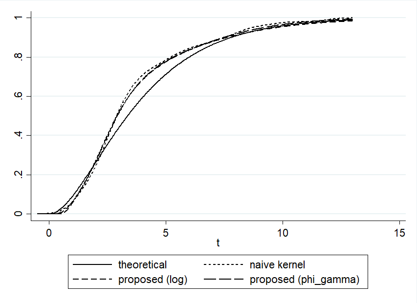
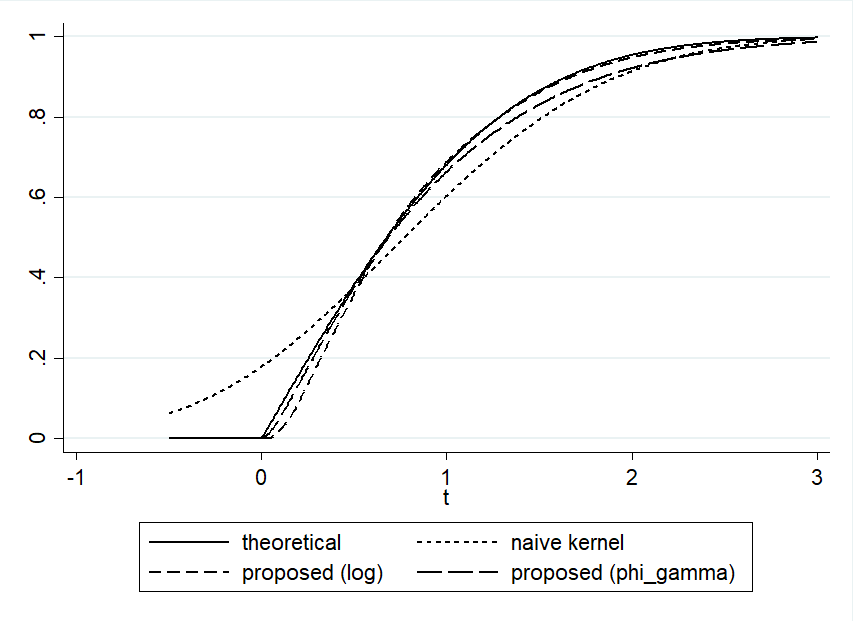
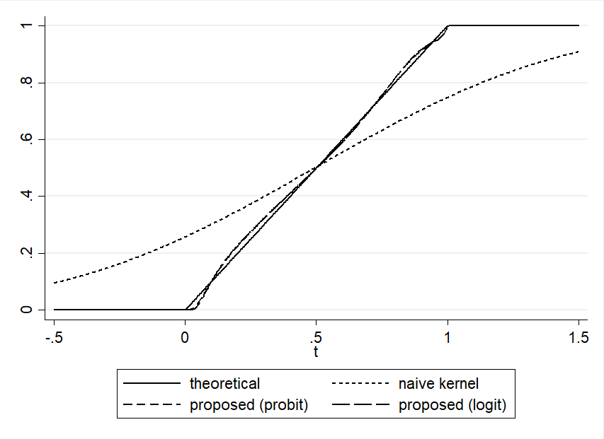
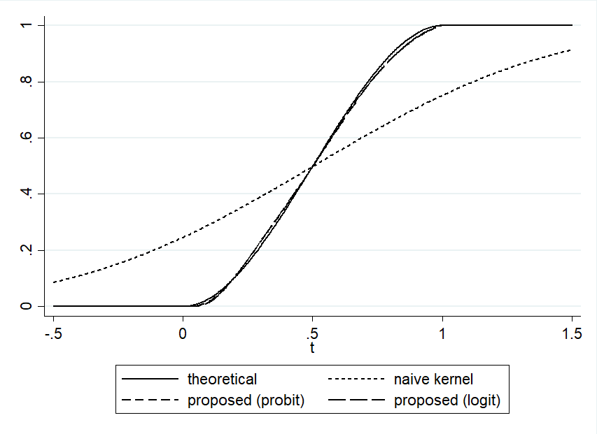
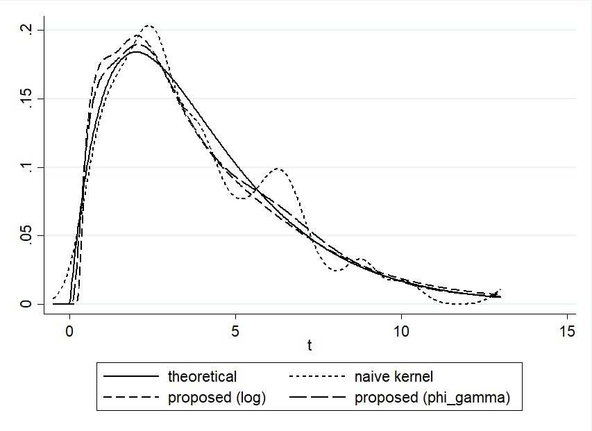
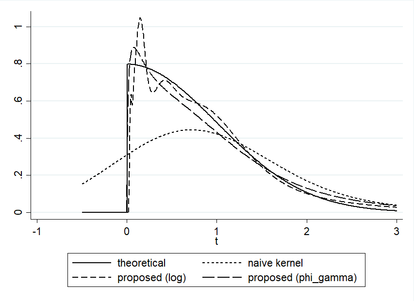
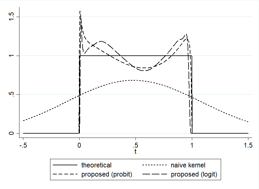
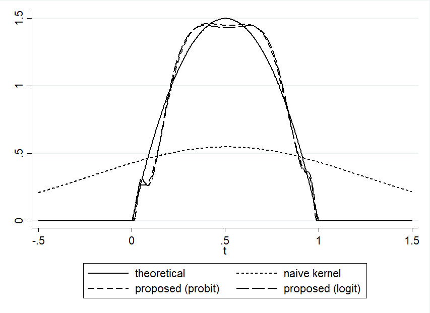
For the simulation to show the performances of the new distribution function estimator, we calculated the average integrated squared error (AISE) and repeated them 100010001000 times for each case. We compared the naive kernel distribution function estimator F^Xsubscript^𝐹𝑋\widehat{F}_{X} and our proposed estimator F~Xsubscript~𝐹𝑋\widetilde{F}_{X}. In the case of the proposed method, we chose two mappings g1superscript𝑔1g^{-1} for each case. When Ω=+Ωsuperscript\Omega=\mathbb{R}^{+}, we used the logarithm function log(x)𝑥\log(x) and a composite of two functions Φ1γsuperscriptΦ1𝛾\Phi^{-1}\circ\gamma, where γ(x)=1ex𝛾𝑥1superscript𝑒𝑥\gamma(x)=1-e^{x}. However, if Ω=[0,1]Ω01\Omega=[0,1], we utilized probit and logit functions. With size 505050, the generated samples were drawn from gamma Gamma(2,2)𝐺𝑎𝑚𝑚𝑎22Gamma(2,2), weibull Weibull(2,2)𝑊𝑒𝑖𝑏𝑢𝑙𝑙22Weibull(2,2), standard log-normal log.N(0,1)formulae-sequence𝑁01\log.N(0,1), absolute-normal abs.N(0,1)formulae-sequence𝑎𝑏𝑠𝑁01abs.N(0,1), standard uniform U(0,1)𝑈01U(0,1), and beta distributions with three different sets of parameters (Beta(1,3)𝐵𝑒𝑡𝑎13Beta(1,3), Beta(2,2)𝐵𝑒𝑡𝑎22Beta(2,2), and Beta(3,1)𝐵𝑒𝑡𝑎31Beta(3,1)). The kernel function we used here is the Gaussian Kernel and the bandwidths were chosen by cross-validation technique. We actually did the same simulation study using the Epanechnikov Kernel, but the results are quite similar. Graphs of some chosen cases are shown as well in Figure 1.

Table 1: AISE (×105absentsuperscript105\times 10^{5}) comparison of DF estimators
Distributions F^Xsubscript^𝐹𝑋\widehat{F}_{X} F~logsubscript~𝐹\widetilde{F}_{\log} F~Φ1γsubscript~𝐹superscriptΦ1𝛾\widetilde{F}_{\Phi^{-1}\circ\gamma} F~probitsubscript~𝐹𝑝𝑟𝑜𝑏𝑖𝑡\widetilde{F}_{probit} F~logitsubscript~𝐹𝑙𝑜𝑔𝑖𝑡\widetilde{F}_{logit}
Gamma(2,2)𝐺𝑎𝑚𝑚𝑎22Gamma(2,2) 246924692469 225322532253 𝟐𝟏𝟖𝟏2181\mathbf{2181} - -
Weibull(2,2)𝑊𝑒𝑖𝑏𝑢𝑙𝑙22Weibull(2,2) 222422242224 𝟏𝟎𝟎𝟑1003\mathbf{1003} 135013501350 - -
log.N(0,1)formulae-sequence𝑁01\log.N(0,1) 178417841784 126412641264 𝟏𝟐𝟓𝟒1254\mathbf{1254} - -
abs.N(0,1)formulae-sequence𝑎𝑏𝑠𝑁01abs.N(0,1) 251725172517 𝟓𝟒𝟒544\mathbf{544} 727727727 - -
U(0,1)𝑈01U(0,1) 507450745074 - - 𝟐𝟒𝟔246\mathbf{246} 248248248
Beta(1,3)𝐵𝑒𝑡𝑎13Beta(1,3) 781078107810 - - 𝟏𝟕𝟎170\mathbf{170} 172172172
Beta(2,2)𝐵𝑒𝑡𝑎22Beta(2,2) 674667466746 - - 𝟏𝟖𝟓185\mathbf{185} 188188188
Beta(3,1)𝐵𝑒𝑡𝑎31Beta(3,1) 780178017801 - - 𝟏𝟓𝟒154\mathbf{154} 156156156
Refer to caption
(a) XGamma(2,2)similar-to𝑋𝐺𝑎𝑚𝑚𝑎22X\sim Gamma(2,2)
Refer to caption
(b) Xabs.N(0,1)formulae-sequencesimilar-to𝑋𝑎𝑏𝑠𝑁01X\sim abs.N(0,1)
Refer to caption
(c) XU(0,1)similar-to𝑋𝑈01X\sim U(0,1)
Refer to caption
(d) XBeta(2,2)similar-to𝑋𝐵𝑒𝑡𝑎22X\sim Beta(2,2)
Figure 1: Graphs comparisons of FX(x)subscript𝐹𝑋𝑥F_{X}(x), F^X(x)subscript^𝐹𝑋𝑥\widehat{F}_{X}(x), and F~X(x)subscript~𝐹𝑋𝑥\widetilde{F}_{X}(x) for several distributions, with sample size n=50𝑛50n=50.

As we can see in Table 1, our proposed estimator outperformed the naive kernel distribution function. Though the differences are not so big in the cases of gamma, weibull, and the log-normal distributions, but the gaps are glaring in the absolute-normal case or when the support of the distributions is the unit interval. The cause of this phenomena might be seen in Figure 1.

Albeit the shapes of F~logsubscript~𝐹\widetilde{F}_{\log} and F~Φ1γsubscript~𝐹superscriptΦ1𝛾\widetilde{F}_{\Phi^{-1}\circ\gamma} are more similar to the theoretical distribution in Figure 1(a), but we have to admit that the shape of F^Xsubscript^𝐹𝑋\widehat{F}_{X} is not so much different with the rests. However in Figure 1(b), (c), and (d), it is obvious that the naive kernel distribution function is too far-off the mark, particularly in the case of Ω=[0,1]Ω01\Omega=[0,1]. As the absolute-normal, uniform, and beta distributions have quite high probability density near the boundary point x=0𝑥0x=0 (also x=1𝑥1x=1 for unit interval case), the naive kernel estimator spreads this "high density information" around the boundary regions. However, since F^Xsubscript^𝐹𝑋\widehat{F}_{X} cannot detect the boundaries, it puts this "high density information" outside the support as well. This is not happening too severely in the case of Figure 1(a) because the probability density near x=0𝑥0x=0 is fairly low. Hence, although the value of F^X(x)subscript^𝐹𝑋𝑥\widehat{F}_{X}(x) might be still positive when x0𝑥superscript0x\approx 0^{-}, but it is not so far from 00 and vanishes quickly

Remark 4.1

Figure 1(c) and (d) also gave a red-alert if we try to use the naive kernel distribution function in place of empirical distribution for goodness-of-fit tests. As the shapes of F^Xsubscript^𝐹𝑋\widehat{F}_{X} in Figure 1(c) and (d) resemble the normal distribution function a lot, if we test H0:XN(μ,σ2):subscript𝐻0similar-to𝑋𝑁𝜇superscript𝜎2H_{0}:X\sim N(\mu,\sigma^{2}), we will find the tests may not reject the null hypothesis. This shall cause the increment of type-2 error.

Remark 4.2

It is worth to note that in Table 1, even though F~probitsubscript~𝐹𝑝𝑟𝑜𝑏𝑖𝑡\widetilde{F}_{probit} performed better, but its differences are too little to claim that it outperformed F~logitsubscript~𝐹𝑙𝑜𝑔𝑖𝑡\widetilde{F}_{logit}. From here we can conclude that probit and logit functions work pretty much the same for F~Xsubscript~𝐹𝑋\widetilde{F}_{X}.

Since we introduced f^Xsubscript^𝑓𝑋\widehat{f}_{X} as a new boundary-free kernel density estimator, we also provide some illustrations of its performances in this subsection. Under the same settings as in the simulation study of the distribution function case, we can see the results of its simulation in Table 2 and Figure 2.

Table 2: AISE (×105absentsuperscript105\times 10^{5}) comparison of density estimators
Distributions f^Xsubscript^𝑓𝑋\widehat{f}_{X} f~logsubscript~𝑓\widetilde{f}_{\log} f~Φ1γsubscript~𝑓superscriptΦ1𝛾\widetilde{f}_{\Phi^{-1}\circ\gamma} f~probitsubscript~𝑓𝑝𝑟𝑜𝑏𝑖𝑡\widetilde{f}_{probit} f~logitsubscript~𝑓𝑙𝑜𝑔𝑖𝑡\widetilde{f}_{logit}
Gamma(2,2)𝐺𝑎𝑚𝑚𝑎22Gamma(2,2) 925925925 744744744 𝟔𝟐𝟒624\mathbf{624} - -
Weibull(2,2)𝑊𝑒𝑖𝑏𝑢𝑙𝑙22Weibull(2,2) 661666166616 𝟑𝟕𝟗𝟗3799\mathbf{3799} 398639863986 - -
log.N(0,1)formulae-sequence𝑁01\log.N(0,1) 741674167416 356935693569 𝟐𝟔𝟑𝟖2638\mathbf{2638} - -
abs.N(0,1)formulae-sequence𝑎𝑏𝑠𝑁01abs.N(0,1) 480054800548005 344963449634496 𝟏𝟒𝟓𝟔𝟑14563\mathbf{14563} - -
U(0,1)𝑈01U(0,1) 369453694536945 - - 𝟏𝟒𝟐𝟑𝟓14235\mathbf{14235} 213252132521325
Beta(1,3)𝐵𝑒𝑡𝑎13Beta(1,3) 109991109991109991 - - 𝟏𝟖𝟏𝟗𝟗18199\mathbf{18199} 281792817928179
Beta(2,2)𝐵𝑒𝑡𝑎22Beta(2,2) 525255252552525 - - 𝟓𝟓𝟏𝟒5514\mathbf{5514} 605260526052
Beta(3,1)𝐵𝑒𝑡𝑎31Beta(3,1) 109999109999109999 - - 𝟏𝟕𝟑𝟓𝟑17353\mathbf{17353} 289352893528935
Refer to caption
(a) XGamma(2,2)similar-to𝑋𝐺𝑎𝑚𝑚𝑎22X\sim Gamma(2,2)
Refer to caption
(b) Xabs.N(0,1)formulae-sequencesimilar-to𝑋𝑎𝑏𝑠𝑁01X\sim abs.N(0,1)
Refer to caption
(c) XU(0,1)similar-to𝑋𝑈01X\sim U(0,1)
Refer to caption
(d) XBeta(2,2)similar-to𝑋𝐵𝑒𝑡𝑎22X\sim Beta(2,2)
Figure 2: Graphs comparisons of fX(x)subscript𝑓𝑋𝑥f_{X}(x), f^X(x)subscript^𝑓𝑋𝑥\widehat{f}_{X}(x), and f~X(x)subscript~𝑓𝑋𝑥\widetilde{f}_{X}(x) for several distributions, with sample size n=50𝑛50n=50.

From AISE point of view, once again our proposed estimator outperformed the naive kernel one, and huge gaps happened as well when the support of the distribution is the unit interval. We may take some interests in Figure 2(b), (c), and (d), as the graphs of F^Xsubscript^𝐹𝑋\widehat{F}_{X} are too different with the theoretical ones, and more similar to the gaussian bell shapes instead. This situation resonates with our claim in Remark 4.1.

4.2 boundary-free kernel-type KS and CvM tests simulations

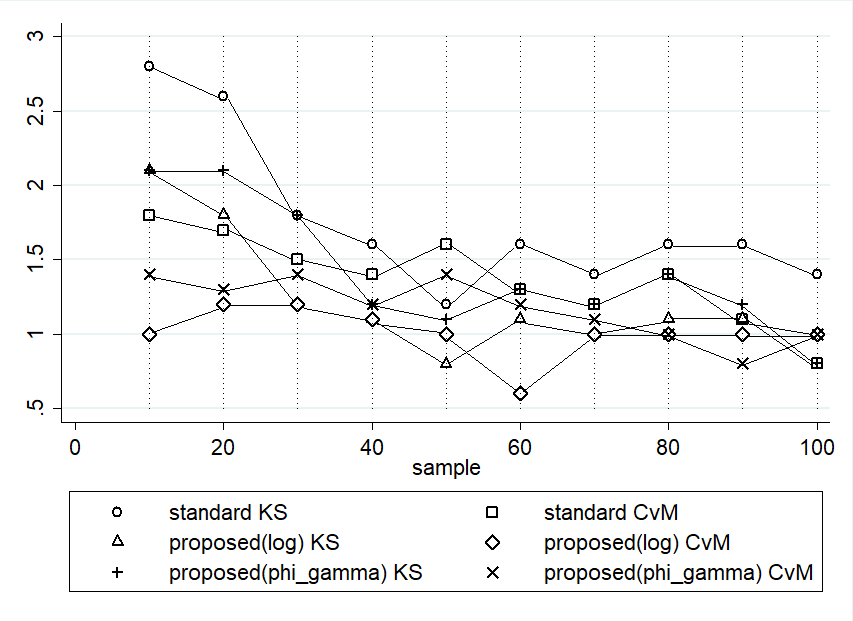
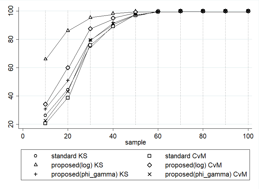
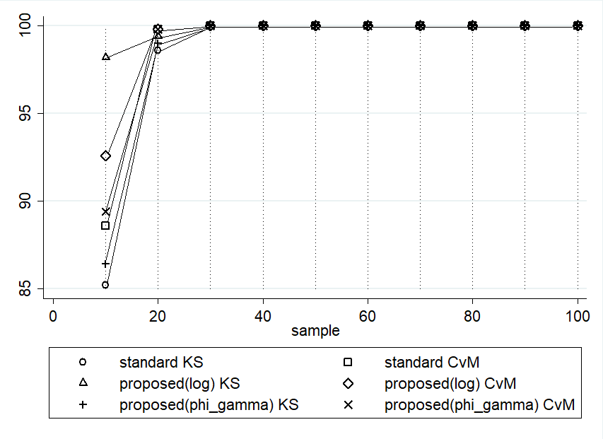
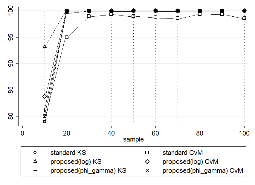
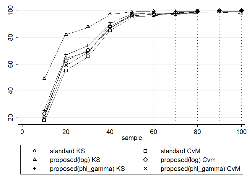
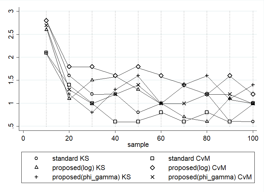
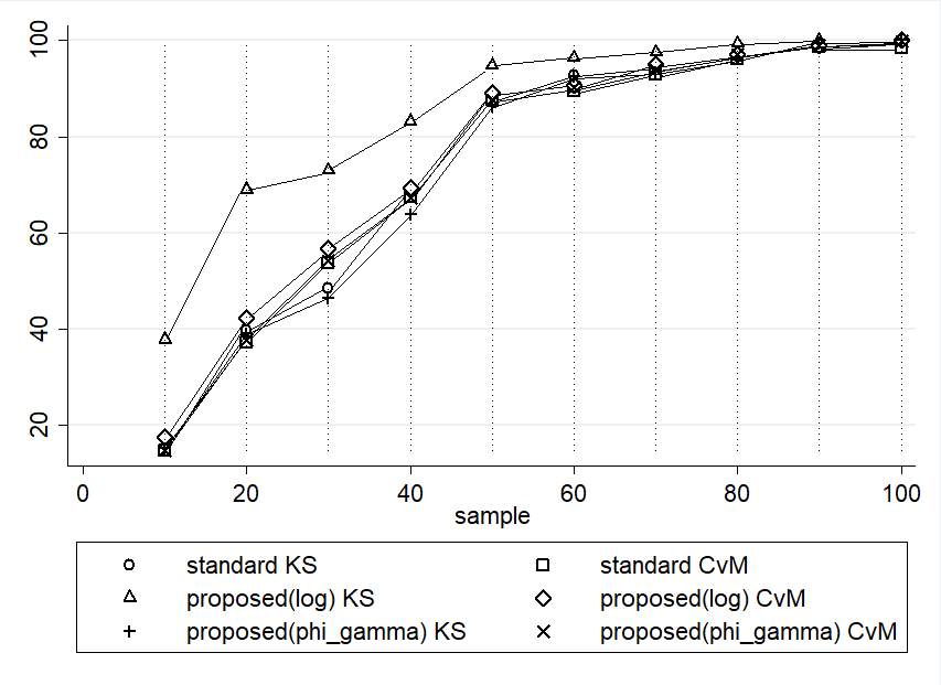
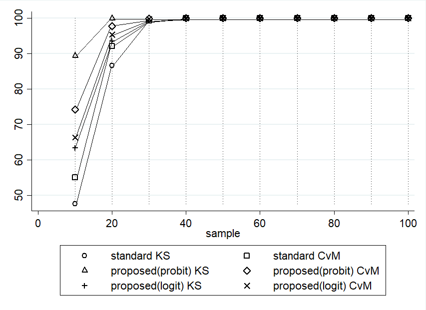
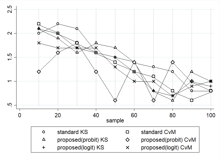
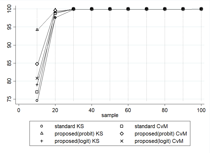
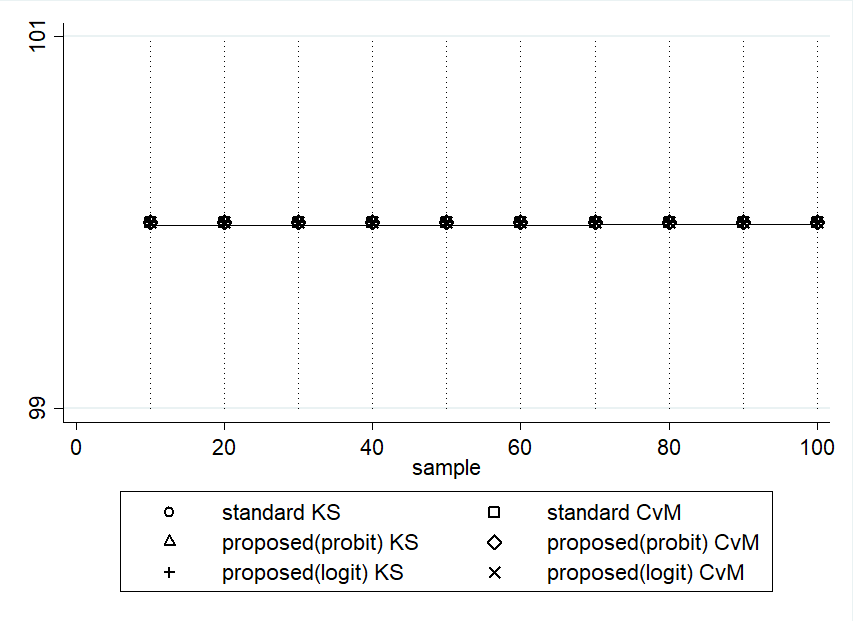
We provide the results of our simulation studies regarding the new Kolmogorov-Smirnov and Cramér-von Mises tests in this part. As a measure of comparison, we calculated the percentage of rejecting several null hypothesis when the samples were drawn from certain distributions. When the actual distribution and the null hypothesis are same, we expect the percentage should be close to 100α%100percent𝛼100\alpha\% (significance level in percent). However, if the real distribution does not match the H0subscript𝐻0H_{0}, we hope to see the percentage is as large as possible. To illustrate how the behaviours of the statistics change, we generated a sequential numbers of sample sizes, started from 101010 until 100100100, with 100010001000 repetitions for each case. We chose level of significance α=0.01𝛼0.01\alpha=0.01, and we compared the standard KS and CvM tests with our proposed tests.

Refer to caption
(a) H0:Gamma(2,2):subscript𝐻0𝐺𝑎𝑚𝑚𝑎22H_{0}:Gamma(2,2)
Refer to caption
(b) H0:Weibull(2,2):subscript𝐻0𝑊𝑒𝑖𝑏𝑢𝑙𝑙22H_{0}:Weibull(2,2)
Refer to caption
(c) H0:log.N(0,1)H_{0}:\log.N(0,1)
Refer to caption
(d) H0:abs.N(0,1)H_{0}:abs.N(0,1)
Figure 3: Simulated percentage (%) of rejecting null hypothesis when the samples were drawn from Weibull(2,2)𝑊𝑒𝑖𝑏𝑢𝑙𝑙22Weibull(2,2).

From Figure 3, we see that the modified KS and CvM tests outperformed the standard ones, especially the proposed KS test with logarithm as the bijective transformation. From Figure 3(a), (c), and (d), KS test with log\log function has the highest percentage of rejecting H0subscript𝐻0H_{0} even when the sample sizes were still 101010. However, even though the new CvM test with logarithmic function was always the second highest in the beginning, CvM~logsubscript~𝐶𝑣𝑀\widetilde{CvM}_{\log} was also the first one that reached 100%percent100100\%. On the other hand, based on Figure 3(b) we can say all statistical tests (standard and proposed) were having similar stable behaviours, as their numbers were still in the interval 0.5%2%percent0.5percent20.5\%-2\%. However at this time, CvM~logsubscript~𝐶𝑣𝑀\widetilde{CvM}_{\log} performed slightly better than the others, because its numbers in general were the closest to 1%percent11\%.

Refer to caption
(a) H0:Gamma(2,2):subscript𝐻0𝐺𝑎𝑚𝑚𝑎22H_{0}:Gamma(2,2)
Refer to caption
(b) H0:Weibull(2,2):subscript𝐻0𝑊𝑒𝑖𝑏𝑢𝑙𝑙22H_{0}:Weibull(2,2)
Refer to caption
(c) H0:log.N(0,1)H_{0}:\log.N(0,1)
Refer to caption
(d) H0:abs.N(0,1)H_{0}:abs.N(0,1)
Figure 4: Simulated percentage (%) of rejecting null hypothesis when the samples were drawn from log.N(0,1)formulae-sequence𝑁01\log.N(0,1).

Similar things happened when we drew the samples from the standard log-normal distribution, which our proposed methods outperformed the standard ones. However this time, the modified KS test with g1=logsuperscript𝑔1g^{-1}=\log always gave the best results. Yet, we may take some notes from Figure 4. First, although when n=10𝑛10n=10 all the percentages were far from 1%percent11\% in Figure 4(c), but after n=20𝑛20n=20 every tests went stable inside 0.5%2%percent0.5percent20.5\%-2\% interval. Second, as seen in Figure 4(d), it seems difficult to reject H0:abs.N(0,1)H_{0}:abs.N(0,1) when the actual distribution is log.N(0,1)formulae-sequence𝑁01\log.N(0,1), even KS~logsubscript~𝐾𝑆\widetilde{KS}_{\log} could only reach 100%percent100100\% rejection after n=80𝑛80n=80. While, on the other hand, it was quite easy to reject H0:Gamma(2,2):subscript𝐻0𝐺𝑎𝑚𝑚𝑎22H_{0}:Gamma(2,2) as most of the tests already reached 100%percent100100\% rejection when n=20𝑛20n=20 (similar to Figure 3(a)).

Refer to caption
(a) H0:U(0,1):subscript𝐻0𝑈01H_{0}:U(0,1)
Refer to caption
(b) H0:Beta(1,3):subscript𝐻0𝐵𝑒𝑡𝑎13H_{0}:Beta(1,3)
Refer to caption
(c) H0:Beta(2,2):subscript𝐻0𝐵𝑒𝑡𝑎22H_{0}:Beta(2,2)
Refer to caption
(d) H0:Beta(3,1):subscript𝐻0𝐵𝑒𝑡𝑎31H_{0}:Beta(3,1)
Figure 5: Simulated percentage (%) of rejecting null hypothesis when the samples were drawn from Beta(1,3)𝐵𝑒𝑡𝑎13Beta(1,3).

Something more extreme happened in Figure 5, as all of the tests could reach 100% rejection rate since n=30𝑛30n=30, even since n=10𝑛10n=10 in Figure 5(d). Though seems strange, the cause of this phenomenon is obvious. The shape of the distribution function of Beta(1,3)𝐵𝑒𝑡𝑎13Beta(1,3) is so different with other three distributions in this study, especially with Beta(3,1)𝐵𝑒𝑡𝑎31Beta(3,1). Hence, even with small sample size, the tests could reject the false null hypothesis. However, we still are able to claim that our proposed tests worked better than the standard goodness-of-fit tests, because before all the tests reached 100% point, the standard KS and CvM tests had the lowest percentages.

From this numerical studies, we can conclude that both the standard and the proposed KS and CvM tests will give the same result when the sample size is large. However, if the sample size is small, our proposed methods will give better and more reliable results.

5 Conclusion

This article has proposed new boundary-free kernel-smoothed Kolmogorov-Smirnov and Cramér-von Mises tests when the data is supported on a proper subset of the real line. First we constructed a new boundary-free estimator of the distribution function using bijective transformations (we also intriduced a new boundary-free density estimator). After deriving the formulas of the bias and the variance of the estimator, we defined the new goodness-of-fit tests. The properties of our proposed methods have been discovered and discussed. Moreover, the results of the numerical studies reveal superior performances of the proposed methods.

Bibliography

Abdous, B. 1993. Note on the minimum mean integrated squared error of kernel estimates of a distribution function and its derivatives. Communications in Statistics – Theory and Methods 22: 603–609. doi: 10.1080/03610929308831040

Antoneli, F. et al. 2018. A Kolmogorov-Smirnov test for the molecular clock based on bayesian ensembles of phylogenies. PLoS ONE 13(1): e0190826. doi: 10.1371/journal.pone.0190826

Azzalini, A. 1981. A note on the estimation of a distribution function and quantiles by a kernel method. Biometrika 68: 326–328. doi: 10.2307/2335836

Baringhaus, L. and N. Henze. 2017. Cramér-von Mises distance: Probabilistic interpretation, confidence intervals, and neighbourhood-of-model validation. Journal of Nonparametric Statistics 29: 167–188. doi: 10.1080/10485252.2017.1285029

Chen, H., M. Döring, and U. Jensen. 2018. Test for model selection using Cramér-von Mises distance in a fixed design regression setting. AStA Advances in Statistical Analysis 102: 505–535. doi: 10.1007/s10182-017-0317-0

Cowling, A., and P. Hall. 1996. On pseudodata methods for removing boundary effects in kernel density estimation. Journal of the Royal Statistical Society B 58: 551–563. doi: 10.2307/2345893

Curry, J., X. Dang, and H. Sang. 2019. A rank-based Cramér-von-Mises-type test for two samples. Brazilian Journal of Probability and Statistics 33(3): 425–454. doi: 10.1214/18-BJPS396

Evans. D. L., J. H. Drew, and L. M. Leemis. 2017. The distribution of the Kolmogorov-Smirnov, Cramer-von Mises, and Anderson-Darling test statistics for exponential populations with estimated parameters. Computational Probability Applications 247: 165–190. doi: 10.1007/978-3-319-43317-2_13

Falk, M. 1983. Relative efficiency and deficiency of kernel type estimators of smooth distribution functions. Statistica Neerlandica 37: 73–83. doi: 10.1111/j.1467-9574.1983.tb00802.x

Finner, H., and V. Gontscharuk. 2018. Two-sample Kolmogorov-Smirnov-type tests revisited: Old and new tests in terms of local levels. Annals of Statistics 46(6A): 3014–3037. doi:10.1214/17-AOS1647

Hall, P., and T. E. Wehrly. 1991. A geometrical method for removing edge effects from kernel-type nonparametric regression estimators. Journal of the American Statistical Association 86: 665–672. doi: 10.1080/01621459.1991.10475092

Hill, P. D. 1985. Kernel estimation of a distribution function. Communications in Statistics – Theory and Methods 14: 605–620. doi: 10.1080/03610928508828937

Jones, M. C., and P. J. Foster. 1996. A simple nonnegative boundary correction method for kernel density estimation. Statistica Sinica 6: 1005–1013

Loeve, M (1963) Probability Theory. New Jersey: Van Nostrand-Reinhold.

Müller, H. G. 1991. Smooth optimum kernel estimators near endpoints. Biometrika 78: 521–530. doi: 10.1093/biomet/78.3.521

Müller, H. G. 1993. On the boundary kernel method for nonparametric curve estimation near endpoints. Scandinavian Journal of Statistics 20: 313–328

Müller, H. G., and J. L. Wang. 1994. Hazard rate estimation under random censoring with varying kernels and bandwidths. Biometrics 50: 61–76. doi: 10.2307/2533197

Nadaraya, E. A. 1964. Some new estimates for distribution functions. Theory of Probability and Its Applications 9: 497–500. doi: 10.1137/1109069

Omelka, M., I. Gijbels, and N. Veraverbeke. 2009. Improved kernel estimation of copulas: weak convergence and goodness-of-fit testing. Annals of Statistics 37: 3023–3058. doi: 10.1214/08-AOS666

Reiss, R. D. 1981. Nonparametric estimation of smooth distribution functions. Scandinavian Journal of Statistics 8(2): 116–119

Schuster, E. F. 1985. Incorporating support constraints into nonparametric estimators of densities. Communication in Statistics – Theory and Methods 14: 1123-–1136. doi: 10.1080/03610928508828965

Shirahata, S., and I. S. Chu. 1992. Integrated squared error of kernel type estimator of distribution function. Annals of the Institute of Statistical Mathematics 44: 579–591. doi: 10.1007/BF00050707

Singh, R. S., T. Gasser, and B. Prasad. 1983. Nonparametric estimates of distribution functions. Communications in Statistics – Theory and Methods 12: 2095–2108. doi: 10.1080/03610928308828593

Swanepoel, J. W. H. 1988. Mean integrated squared error properties and optimal kernels when estimating a distribution function. Communications in Statistics – Theory and Methods 17: 3785–3799. doi: 10.1080/03610928808829835

Watson, G. S., and M. R. Leadbetter. 1964. Hazard analysis 2. Sankhyā: The Indian Journal of Statistics, Series A 26: 101–106

Winter, B. B. 1973. Strong uniform consistency of integrals of density estimators. Canadian Journal of Statistics 1: 247–253. doi: 10.2307/3315003

Yamato, H. 1973. Uniform convergence of an estimator of a distribution function. Bulletin of Mathematical Statistics 15: 69–78

Yukich, J. E. 1989. A note on limit theorems for perturbed empirical processes. Stochastic Process and Applications 33: 163–173. doi: 10.1016/0304-4149(89)90073-2

Zierk, J. et al. 2020. Reference interval estimation from mixed distributions using truncation points and the Kolmogorov-Smirnov distance (kosmic). Scientific Reports 10: 1704. doi: 10.1038/s41598-020-58749-2

Appendix

proof of theorem 2.1

Utilizing the usual reasoning of i.i.d. random variables and the transformation property of expectation, with Y=g1(X1)𝑌superscript𝑔1subscript𝑋1Y=g^{-1}(X_{1}), we have

E[F~X(x)]𝐸delimited-[]subscript~𝐹𝑋𝑥\displaystyle E[\widetilde{F}_{X}(x)] =\displaystyle= W(g1(x)yh)fY(y)dysuperscriptsubscript𝑊superscript𝑔1𝑥𝑦subscript𝑓𝑌𝑦differential-d𝑦\displaystyle\int_{-\infty}^{\infty}W\left(\frac{g^{-1}(x)-y}{h}\right)f_{Y}(y)\mathrm{d}y
=\displaystyle= 1hFY(y)K(g1(x)yh)dy1superscriptsubscriptsubscript𝐹𝑌𝑦𝐾superscript𝑔1𝑥𝑦differential-d𝑦\displaystyle\frac{1}{h}\int_{-\infty}^{\infty}F_{Y}(y)K\left(\frac{g^{-1}(x)-y}{h}\right)\mathrm{d}y
=\displaystyle= FY(g1(x)hv)K(v)dvsuperscriptsubscriptsubscript𝐹𝑌superscript𝑔1𝑥𝑣𝐾𝑣differential-d𝑣\displaystyle\int_{-\infty}^{\infty}F_{Y}(g^{-1}(x)-hv)K(v)\mathrm{d}v
=\displaystyle= [FY(g1(x))hvfY(g1(x))+h22v2fY(g1(x))+o(h2)]K(v)dvsuperscriptsubscriptdelimited-[]subscript𝐹𝑌superscript𝑔1𝑥𝑣subscript𝑓𝑌superscript𝑔1𝑥superscript22superscript𝑣2superscriptsubscript𝑓𝑌superscript𝑔1𝑥𝑜superscript2𝐾𝑣differential-d𝑣\displaystyle\int_{-\infty}^{\infty}\left[F_{Y}(g^{-1}(x))-hvf_{Y}(g^{-1}(x))+\frac{h^{2}}{2}v^{2}f_{Y}^{\prime}(g^{-1}(x))+o(h^{2})\right]K(v)\mathrm{d}v
=\displaystyle= FX(x)+h22c1(x)v2K(v)dv+o(h2),subscript𝐹𝑋𝑥superscript22subscript𝑐1𝑥superscriptsubscriptsuperscript𝑣2𝐾𝑣differential-d𝑣𝑜superscript2\displaystyle F_{X}(x)+\frac{h^{2}}{2}c_{1}(x)\int_{-\infty}^{\infty}v^{2}K(v)\mathrm{d}v+o(h^{2}),

and we obtained the Bias[F~X(x)]𝐵𝑖𝑎𝑠delimited-[]subscript~𝐹𝑋𝑥Bias[\widetilde{F}_{X}(x)]. For the variance of F~X(x)subscript~𝐹𝑋𝑥\widetilde{F}_{X}(x), we first calculate

E[W2(g1(x)g1(X1)h)]𝐸delimited-[]superscript𝑊2superscript𝑔1𝑥superscript𝑔1subscript𝑋1\displaystyle E\left[W^{2}\left(\frac{g^{-1}(x)-g^{-1}(X_{1})}{h}\right)\right] =\displaystyle= 2hFY(y)W(g1(x)yh)K(g1(x)yh)dy2superscriptsubscriptsubscript𝐹𝑌𝑦𝑊superscript𝑔1𝑥𝑦𝐾superscript𝑔1𝑥𝑦differential-d𝑦\displaystyle\frac{2}{h}\int_{-\infty}^{\infty}F_{Y}(y)W\left(\frac{g^{-1}(x)-y}{h}\right)K\left(\frac{g^{-1}(x)-y}{h}\right)\mathrm{d}y
=\displaystyle= 2[FY(g1(x))hvfY(g1(x))+o(h)]W(v)K(v)dv2superscriptsubscriptdelimited-[]subscript𝐹𝑌superscript𝑔1𝑥𝑣subscript𝑓𝑌superscript𝑔1𝑥𝑜𝑊𝑣𝐾𝑣differential-d𝑣\displaystyle 2\int_{-\infty}^{\infty}[F_{Y}(g^{-1}(x))-hvf_{Y}(g^{-1}(x))+o(h)]W(v)K(v)\mathrm{d}v
=\displaystyle= FX(x)2hg(g1(x))fX(x)r1+o(h),subscript𝐹𝑋𝑥2superscript𝑔superscript𝑔1𝑥subscript𝑓𝑋𝑥subscript𝑟1𝑜\displaystyle F_{X}(x)-2hg^{\prime}(g^{-1}(x))f_{X}(x)r_{1}+o(h),

and we got the variance.

proof of theorem 2.3

For some δ>0𝛿0\delta>0, using Hölder and Cramér crsubscript𝑐𝑟c_{r} inequalities, we have

E[|W(g1(x)g1(X1)h)E{W(g1(x)g1(X1)h)}|2+δ]𝐸delimited-[]superscript𝑊superscript𝑔1𝑥superscript𝑔1subscript𝑋1𝐸𝑊superscript𝑔1𝑥superscript𝑔1subscript𝑋12𝛿\displaystyle E\left[\left|W\left(\frac{g^{-1}(x)-g^{-1}(X_{1})}{h}\right)-E\left\{W\left(\frac{g^{-1}(x)-g^{-1}(X_{1})}{h}\right)\right\}\right|^{2+\delta}\right]
22+δE[|W(g1(x)g1(X1)h)|2+δ].absentsuperscript22𝛿𝐸delimited-[]superscript𝑊superscript𝑔1𝑥superscript𝑔1subscript𝑋12𝛿\displaystyle\leq 2^{2+\delta}E\left[\left|W\left(\frac{g^{-1}(x)-g^{-1}(X_{1})}{h}\right)\right|^{2+\delta}\right].

But, since 0W(v)10𝑊𝑣10\leq W(v)\leq 1 for any v𝑣v\in\mathbb{R}, then

E[|W(g1(x)g1(X1)h)E{W(g1(x)g1(X1)h)}|2+δ]22+δ<.𝐸delimited-[]superscript𝑊superscript𝑔1𝑥superscript𝑔1subscript𝑋1𝐸𝑊superscript𝑔1𝑥superscript𝑔1subscript𝑋12𝛿superscript22𝛿\displaystyle E\left[\left|W\left(\frac{g^{-1}(x)-g^{-1}(X_{1})}{h}\right)-E\left\{W\left(\frac{g^{-1}(x)-g^{-1}(X_{1})}{h}\right)\right\}\right|^{2+\delta}\right]\leq 2^{2+\delta}<\infty.

Also, because Var[W(g1(x)g1(X1)h)]=O(1)𝑉𝑎𝑟delimited-[]𝑊superscript𝑔1𝑥superscript𝑔1subscript𝑋1𝑂1Var\left[W\left(\frac{g^{-1}(x)-g^{-1}(X_{1})}{h}\right)\right]=O(1), we get

E[|W(g1(x)g1(X1)h)E{W(g1(x)g1(X1)h)}|2+δ]nδ/2[Var{W(g1(x)g1(X1)h)}]1+δ/20𝐸delimited-[]superscript𝑊superscript𝑔1𝑥superscript𝑔1subscript𝑋1𝐸𝑊superscript𝑔1𝑥superscript𝑔1subscript𝑋12𝛿superscript𝑛𝛿2superscriptdelimited-[]𝑉𝑎𝑟𝑊superscript𝑔1𝑥superscript𝑔1subscript𝑋11𝛿20\displaystyle\frac{E\left[\left|W\left(\frac{g^{-1}(x)-g^{-1}(X_{1})}{h}\right)-E\left\{W\left(\frac{g^{-1}(x)-g^{-1}(X_{1})}{h}\right)\right\}\right|^{2+\delta}\right]}{n^{\delta/2}\left[Var\left\{W\left(\frac{g^{-1}(x)-g^{-1}(X_{1})}{h}\right)\right\}\right]^{1+\delta/2}}\rightarrow 0

when n𝑛n\rightarrow\infty. Hence, by Loeve (1963), and with the fact F~X(x)pFX(x)subscript𝑝subscript~𝐹𝑋𝑥subscript𝐹𝑋𝑥\widetilde{F}_{X}(x)\rightarrow_{p}F_{X}(x), we can conclude its asymptotic normality.

proof of theorem 2.4

Let FYsubscript𝐹𝑌F_{Y} and F^Ysubscript^𝐹𝑌\widehat{F}_{Y} be the distribution function and the naive kernel distribution function estimator, respectively, of Y1,Y2,,Ynsubscript𝑌1subscript𝑌2subscript𝑌𝑛Y_{1},Y_{2},...,Y_{n}, where Yi=g1(Xi)subscript𝑌𝑖superscript𝑔1subscript𝑋𝑖Y_{i}=g^{-1}(X_{i}). Since F^Ysubscript^𝐹𝑌\widehat{F}_{Y} is a naive kernel distribution function, then Nadaraya (1964) guarantees that supy|F^Y(y)FY(y)|a.s.0subscriptformulae-sequence𝑎𝑠subscriptsupremum𝑦subscript^𝐹𝑌𝑦subscript𝐹𝑌𝑦0\sup_{y\in\mathbb{R}}|\widehat{F}_{Y}(y)-F_{Y}(y)|\rightarrow_{a.s.}0, which implies that

supxΩ|F^Y(g1(x))FY(g1(x))|a.s.0.subscriptformulae-sequence𝑎𝑠subscriptsupremum𝑥Ωsubscript^𝐹𝑌superscript𝑔1𝑥subscript𝐹𝑌superscript𝑔1𝑥0\displaystyle\sup_{x\in\Omega}|\widehat{F}_{Y}(g^{-1}(x))-F_{Y}(g^{-1}(x))|\rightarrow_{a.s.}0.

However, because FY(g1(x))=FX(x)subscript𝐹𝑌superscript𝑔1𝑥subscript𝐹𝑋𝑥F_{Y}(g^{-1}(x))=F_{X}(x), and it is clear that F^Y(g1(x))=F~X(x)subscript^𝐹𝑌superscript𝑔1𝑥subscript~𝐹𝑋𝑥\widehat{F}_{Y}(g^{-1}(x))=\widetilde{F}_{X}(x), then this theorem is proven.

proof of theorem 2.5

Using the similar reasoning as in the proof of Theorem 2.1, we have

E[f^X(x)]𝐸delimited-[]subscript^𝑓𝑋𝑥\displaystyle E[\widehat{f}_{X}(x)] =\displaystyle= 1hg(g1(x))K(g1(x)yh)fY(y)dy1superscript𝑔superscript𝑔1𝑥superscriptsubscript𝐾superscript𝑔1𝑥𝑦subscript𝑓𝑌𝑦differential-d𝑦\displaystyle\frac{1}{hg^{\prime}(g^{-1}(x))}\int_{-\infty}^{\infty}K\left(\frac{g^{-1}(x)-y}{h}\right)f_{Y}(y)\mathrm{d}y
=\displaystyle= 1g(g1(x))fY(g1(x)hv)K(v)dv1superscript𝑔superscript𝑔1𝑥superscriptsubscriptsubscript𝑓𝑌superscript𝑔1𝑥𝑣𝐾𝑣differential-d𝑣\displaystyle\frac{1}{g^{\prime}(g^{-1}(x))}\int_{-\infty}^{\infty}f_{Y}(g^{-1}(x)-hv)K(v)\mathrm{d}v
=\displaystyle= fY(g1(x))g(g1(x))+h2fY′′(g1(x))2g(g1(x))v2K(v)dv+o(h2),subscript𝑓𝑌superscript𝑔1𝑥superscript𝑔superscript𝑔1𝑥superscript2superscriptsubscript𝑓𝑌′′superscript𝑔1𝑥2superscript𝑔superscript𝑔1𝑥superscriptsubscriptsuperscript𝑣2𝐾𝑣differential-d𝑣𝑜superscript2\displaystyle\frac{f_{Y}(g^{-1}(x))}{g^{\prime}(g^{-1}(x))}+\frac{h^{2}f_{Y}^{\prime\prime}(g^{-1}(x))}{2g^{\prime}(g^{-1}(x))}\int_{-\infty}^{\infty}v^{2}K(v)\mathrm{d}v+o(h^{2}),

and we obtained the bias formula. For the variance, first we have to calculate

1hg(g1(x))E[K2(g1(x)Yh)]1superscript𝑔superscript𝑔1𝑥𝐸delimited-[]superscript𝐾2superscript𝑔1𝑥𝑌\displaystyle\frac{1}{hg^{\prime}(g^{-1}(x))}E\left[K^{2}\left(\frac{g^{-1}(x)-Y}{h}\right)\right] =\displaystyle= 1g(g1(x))fY(g1(x)hv)K2(v)dv1superscript𝑔superscript𝑔1𝑥superscriptsubscriptsubscript𝑓𝑌superscript𝑔1𝑥𝑣superscript𝐾2𝑣differential-d𝑣\displaystyle\frac{1}{g^{\prime}(g^{-1}(x))}\int_{-\infty}^{\infty}f_{Y}(g^{-1}(x)-hv)K^{2}(v)\mathrm{d}v
=\displaystyle= fX(x)K2(v)dv+o(1),subscript𝑓𝑋𝑥superscriptsubscriptsuperscript𝐾2𝑣differential-d𝑣𝑜1\displaystyle f_{X}(x)\int_{-\infty}^{\infty}K^{2}(v)\mathrm{d}v+o(1),

and the rests are easily done.

proof of theorem 3.2

First, we need to consider the following inequality

|KSnKS~|𝐾subscript𝑆𝑛~𝐾𝑆\displaystyle|KS_{n}-\widetilde{KS}| =\displaystyle= |supvΩ|Fn(v)F(v)|supzΩ|F~X(z)F(z)||subscriptsupremum𝑣Ωsubscript𝐹𝑛𝑣𝐹𝑣subscriptsupremum𝑧Ωsubscript~𝐹𝑋𝑧𝐹𝑧\displaystyle\left|\sup_{v\in\Omega}|F_{n}(v)-F(v)|-\sup_{z\in\Omega}|\widetilde{F}_{X}(z)-F(z)|\right|
\displaystyle\leq supxΩ||Fn(x)F(x)||F~X(x)F(x)||subscriptsupremum𝑥Ωsubscript𝐹𝑛𝑥𝐹𝑥subscript~𝐹𝑋𝑥𝐹𝑥\displaystyle\sup_{x\in\Omega}\left||F_{n}(x)-F(x)|-|\widetilde{F}_{X}(x)-F(x)|\right|
\displaystyle\leq supxΩ|Fn(x)F(x)F~X(x)+F(x)|subscriptsupremum𝑥Ωsubscript𝐹𝑛𝑥𝐹𝑥subscript~𝐹𝑋𝑥𝐹𝑥\displaystyle\sup_{x\in\Omega}|F_{n}(x)-F(x)-\widetilde{F}_{X}(x)+F(x)|
=\displaystyle= supxΩ|F~X(x)Fn(x)|.subscriptsupremum𝑥Ωsubscript~𝐹𝑋𝑥subscript𝐹𝑛𝑥\displaystyle\sup_{x\in\Omega}|\widetilde{F}_{X}(x)-F_{n}(x)|.

Now, let Fn,Ysubscript𝐹𝑛𝑌F_{n,Y} and F^Ysubscript^𝐹𝑌\widehat{F}_{Y} be the empirical distribution function and the naive kernel distribution function estimator, respectively, of Y1,Y2,,Ynsubscript𝑌1subscript𝑌2subscript𝑌𝑛Y_{1},Y_{2},...,Y_{n}, where Yi=g1(Xi)subscript𝑌𝑖superscript𝑔1subscript𝑋𝑖Y_{i}=g^{-1}(X_{i}). Hence, Omelka et al. (2009) guarantees that supy|F^Y(y)Fn,Y(y)|=op(n1/2)subscriptsupremum𝑦subscript^𝐹𝑌𝑦subscript𝐹𝑛𝑌𝑦subscript𝑜𝑝superscript𝑛12\sup_{y\in\mathbb{R}}|\widehat{F}_{Y}(y)-F_{n,Y}(y)|=o_{p}(n^{-1/2}), which further implies that

supxΩ|F^Y(g1(x))Fn,Y(g1(x))|p0subscript𝑝subscriptsupremum𝑥Ωsubscript^𝐹𝑌superscript𝑔1𝑥subscript𝐹𝑛𝑌superscript𝑔1𝑥0\displaystyle\sup_{x\in\Omega}|\widehat{F}_{Y}(g^{-1}(x))-F_{n,Y}(g^{-1}(x))|\rightarrow_{p}0

with rate n1/2superscript𝑛12n^{-1/2}. But, F^Y(g1(x))=F~X(x)subscript^𝐹𝑌superscript𝑔1𝑥subscript~𝐹𝑋𝑥\widehat{F}_{Y}(g^{-1}(x))=\widetilde{F}_{X}(x) and Fn,Y(g1(x))=Fn(x)subscript𝐹𝑛𝑌superscript𝑔1𝑥subscript𝐹𝑛𝑥F_{n,Y}(g^{-1}(x))=F_{n}(x), and the equivalency is proven.

proof of theorem 3.3

In this proof, we assume the bandwidth h=o(n1/4)𝑜superscript𝑛14h=o(n^{-1/4}). Let us define

Δn=n[F~X(x)F(x)]2dF(x)n[Fn(x)F(x)]2dF(x).subscriptΔ𝑛𝑛superscriptsubscriptsuperscriptdelimited-[]subscript~𝐹𝑋𝑥𝐹𝑥2differential-d𝐹𝑥𝑛superscriptsubscriptsuperscriptdelimited-[]subscript𝐹𝑛𝑥𝐹𝑥2differential-d𝐹𝑥\displaystyle\Delta_{n}=n\int_{-\infty}^{\infty}[\widetilde{F}_{X}(x)-F(x)]^{2}\mathrm{d}F(x)-n\int_{-\infty}^{\infty}[F_{n}(x)-F(x)]^{2}\mathrm{d}F(x).

Then, we have

ΔnsubscriptΔ𝑛\displaystyle\Delta_{n} =\displaystyle= n[F~X(x)F(x)Fn(x)+F(x)][F~X(x)F(x)+Fn(x)F(x)]dF(x)𝑛superscriptsubscriptdelimited-[]subscript~𝐹𝑋𝑥𝐹𝑥subscript𝐹𝑛𝑥𝐹𝑥delimited-[]subscript~𝐹𝑋𝑥𝐹𝑥subscript𝐹𝑛𝑥𝐹𝑥differential-d𝐹𝑥\displaystyle n\int_{-\infty}^{\infty}\left[\widetilde{F}_{X}(x)-F(x)-F_{n}(x)+F(x)\right]\left[\widetilde{F}_{X}(x)-F(x)+F_{n}(x)-F(x)\right]\mathrm{d}F(x)
=\displaystyle= n1ni=1n[Wi(x)Ii(x)]1nj=1n[Wj(x)+Ij(x)]dF(x),𝑛superscriptsubscript1𝑛superscriptsubscript𝑖1𝑛delimited-[]superscriptsubscript𝑊𝑖𝑥superscriptsubscript𝐼𝑖𝑥1𝑛superscriptsubscript𝑗1𝑛delimited-[]superscriptsubscript𝑊𝑗𝑥superscriptsubscript𝐼𝑗𝑥d𝐹𝑥\displaystyle n\int_{-\infty}^{\infty}\frac{1}{n}\sum_{i=1}^{n}\left[W_{i}^{*}(x)-I_{i}^{*}(x)\right]\frac{1}{n}\sum_{j=1}^{n}\left[W_{j}^{*}(x)+I_{j}^{*}(x)\right]\mathrm{d}F(x),

where

Wi(x)=W(g1(x)g1(Xi)h)F(x)andIi(x)=I(Xix)F(x).superscriptsubscript𝑊𝑖𝑥𝑊superscript𝑔1𝑥superscript𝑔1subscript𝑋𝑖𝐹𝑥andsuperscriptsubscript𝐼𝑖𝑥𝐼subscript𝑋𝑖𝑥𝐹𝑥\displaystyle W_{i}^{*}(x)=W\left(\frac{g^{-1}(x)-g^{-1}(X_{i})}{h}\right)-F(x)\;\;\;\mathrm{and}\;\;\;I_{i}^{*}(x)=I(X_{i}\leq x)-F(x).

Note that if ij𝑖𝑗i\neq j, Wi()subscript𝑊𝑖W_{i}(\cdot) and Wj()subscript𝑊𝑗W_{j}(\cdot), also Ii()superscriptsubscript𝐼𝑖I_{i}^{*}(\cdot) and Ij()superscriptsubscript𝐼𝑗I_{j}^{*}(\cdot), are independent.

It follows from the Chauchy-Schwarz Inequality that

E(|Δn|)nE[{1ni=1n(Wi(x)Ii(x))}2]E[{1nj=1n(Wj(x)+Ij(x))}2]dF(x).𝐸subscriptΔ𝑛𝑛superscriptsubscript𝐸delimited-[]superscript1𝑛superscriptsubscript𝑖1𝑛superscriptsubscript𝑊𝑖𝑥superscriptsubscript𝐼𝑖𝑥2𝐸delimited-[]superscript1𝑛superscriptsubscript𝑗1𝑛superscriptsubscript𝑊𝑗𝑥superscriptsubscript𝐼𝑗𝑥2differential-d𝐹𝑥\displaystyle E(|\Delta_{n}|)\leq n\int_{-\infty}^{\infty}\sqrt{E\left[\left\{\frac{1}{n}\sum_{i=1}^{n}(W_{i}^{*}(x)-I_{i}^{*}(x))\right\}^{2}\right]E\left[\left\{\frac{1}{n}\sum_{j=1}^{n}(W_{j}^{*}(x)+I_{j}^{*}(x))\right\}^{2}\right]}\mathrm{d}F(x).

Let us define the bias

bn(x)=E[W(g1(x)g1(Xi)h)]F(x)=O(h2).subscript𝑏𝑛𝑥𝐸delimited-[]𝑊superscript𝑔1𝑥superscript𝑔1subscript𝑋𝑖𝐹𝑥𝑂superscript2\displaystyle b_{n}(x)=E\left[W\left(\frac{g^{-1}(x)-g^{-1}(X_{i})}{h}\right)\right]-F(x)=O(h^{2}).

Hence, it follows from the independence that

E[{1ni=1n(Wi(x)Ii(x))}2]𝐸delimited-[]superscript1𝑛superscriptsubscript𝑖1𝑛superscriptsubscript𝑊𝑖𝑥superscriptsubscript𝐼𝑖𝑥2\displaystyle E\left[\left\{\frac{1}{n}\sum_{i=1}^{n}(W_{i}^{*}(x)-I_{i}^{*}(x))\right\}^{2}\right] =\displaystyle= E[{1ni=1n(Wi(x)bn(x)Ii(x))}2]+bn2(x)𝐸delimited-[]superscript1𝑛superscriptsubscript𝑖1𝑛superscriptsubscript𝑊𝑖𝑥subscript𝑏𝑛𝑥superscriptsubscript𝐼𝑖𝑥2superscriptsubscript𝑏𝑛2𝑥\displaystyle E\left[\left\{\frac{1}{n}\sum_{i=1}^{n}(W_{i}^{*}(x)-b_{n}(x)-I_{i}^{*}(x))\right\}^{2}\right]+b_{n}^{2}(x)
=\displaystyle= 1nE[{W1(x)bn(x)+I1(x)}2]+bn2(x).1𝑛𝐸delimited-[]superscriptsuperscriptsubscript𝑊1𝑥subscript𝑏𝑛𝑥superscriptsubscript𝐼1𝑥2superscriptsubscript𝑏𝑛2𝑥\displaystyle\frac{1}{n}E[\{W_{1}^{*}(x)-b_{n}(x)+I_{1}^{*}(x)\}^{2}]+b_{n}^{2}(x).

Furthermore, we have

E[{W1(x)bn(x)I1(x)}2]𝐸delimited-[]superscriptsuperscriptsubscript𝑊1𝑥subscript𝑏𝑛𝑥superscriptsubscript𝐼1𝑥2\displaystyle E[\{W_{1}^{*}(x)-b_{n}(x)-I_{1}^{*}(x)\}^{2}] =\displaystyle= E[{W1(x)I1(x)}2]2bn(x)E[W1(x)I1(x)]+bn2(x)𝐸delimited-[]superscriptsuperscriptsubscript𝑊1𝑥superscriptsubscript𝐼1𝑥22subscript𝑏𝑛𝑥𝐸delimited-[]superscriptsubscript𝑊1𝑥superscriptsubscript𝐼1𝑥superscriptsubscript𝑏𝑛2𝑥\displaystyle E[\{W_{1}^{*}(x)-I_{1}^{*}(x)\}^{2}]-2b_{n}(x)E[W_{1}^{*}(x)-I_{1}^{*}(x)]+b_{n}^{2}(x)
=\displaystyle= E[{W1(x)}22W1(x)I1(x){I1(x)}2]bn2(x).𝐸delimited-[]superscriptsuperscriptsubscript𝑊1𝑥22superscriptsubscript𝑊1𝑥superscriptsubscript𝐼1𝑥superscriptsuperscriptsubscript𝐼1𝑥2superscriptsubscript𝑏𝑛2𝑥\displaystyle E[\{W_{1}^{*}(x)\}^{2}-2W_{1}^{*}(x)I_{1}^{*}(x)-\{I_{1}^{*}(x)\}^{2}]-b_{n}^{2}(x).

It follows from the mean squared error of F~X(x)subscript~𝐹𝑋𝑥\widetilde{F}_{X}(x) that

E[{W1(x)}2]=F(x)[1F(x)]2hr1g(g1(x))fX(x)+O(h2).𝐸delimited-[]superscriptsuperscriptsubscript𝑊1𝑥2𝐹𝑥delimited-[]1𝐹𝑥2subscript𝑟1superscript𝑔superscript𝑔1𝑥subscript𝑓𝑋𝑥𝑂superscript2\displaystyle E[\{W_{1}^{*}(x)\}^{2}]=F(x)[1-F(x)]-2hr_{1}g^{\prime}(g^{-1}(x))f_{X}(x)+O(h^{2}).

From the definition, we have

E[W1(x)I1(x)]𝐸delimited-[]superscriptsubscript𝑊1𝑥superscriptsubscript𝐼1𝑥\displaystyle E[W_{1}^{*}(x)I_{1}^{*}(x)] =\displaystyle= E[W(g1(x)g1(X1)h)I(X1x)F(x)W(g1(x)g1(X1)h)\displaystyle E\bigg{[}W\left(\frac{g^{-1}(x)-g^{-1}(X_{1})}{h}\right)I(X_{1}\leq x)-F(x)W\left(\frac{g^{-1}(x)-g^{-1}(X_{1})}{h}\right)
F(x)I(X1x)+F2(x)]\displaystyle\;\;\;\;\;\;\;-F(x)I(X_{1}\leq x)+F^{2}(x)\bigg{]}
=\displaystyle= E[W(g1(x)g1(X1)h)I(X1x)]F2(x)bn(x)F(x).𝐸delimited-[]𝑊superscript𝑔1𝑥superscript𝑔1subscript𝑋1𝐼subscript𝑋1𝑥superscript𝐹2𝑥subscript𝑏𝑛𝑥𝐹𝑥\displaystyle E\left[W\left(\frac{g^{-1}(x)-g^{-1}(X_{1})}{h}\right)I(X_{1}\leq x)\right]-F^{2}(x)-b_{n}(x)F(x).

For the first term we have

E[W(g1(x)Yh)I(Yg1(x))]𝐸delimited-[]𝑊superscript𝑔1𝑥𝑌𝐼𝑌superscript𝑔1𝑥\displaystyle E\left[W\left(\frac{g^{-1}(x)-Y}{h}\right)I(Y\leq g^{-1}(x))\right] =\displaystyle= g1(x)W(g1(x)yh)fY(y)dysuperscriptsubscriptsuperscript𝑔1𝑥𝑊superscript𝑔1𝑥𝑦subscript𝑓𝑌𝑦differential-d𝑦\displaystyle\int_{-\infty}^{g^{-1}(x)}W\left(\frac{g^{-1}(x)-y}{h}\right)f_{Y}(y)\mathrm{d}y
=\displaystyle= W(0)FY(g1(x))+0FY(g1(x)hv)K(v)𝑑v𝑊0subscript𝐹𝑌superscript𝑔1𝑥superscriptsubscript0subscript𝐹𝑌superscript𝑔1𝑥𝑣𝐾𝑣differential-d𝑣\displaystyle W(0)F_{Y}(g^{-1}(x))+\int_{0}^{\infty}F_{Y}(g^{-1}(x)-hv)K(v)dv
=\displaystyle= W(0)F(x)+F(x)0K(v)𝑑v+O(h).𝑊0𝐹𝑥𝐹𝑥superscriptsubscript0𝐾𝑣differential-d𝑣𝑂\displaystyle W(0)F(x)+F(x)\int_{0}^{\infty}K(v)dv+O(h).

Since K()𝐾K(\cdot) is symmetric around the origin, we have W(0)=1/2𝑊012W(0)=1/2. Thus, we get

E[W1(x)I1(x)]=F(x)[1F(x)]+O(h).𝐸delimited-[]superscriptsubscript𝑊1𝑥superscriptsubscript𝐼1𝑥𝐹𝑥delimited-[]1𝐹𝑥𝑂\displaystyle E[W_{1}^{*}(x)I_{1}^{*}(x)]=F(x)[1-F(x)]+O(h).

Next we will evaluate E[{n1i=1n(Wi(x)+Ii(x))}2]𝐸delimited-[]superscriptsuperscript𝑛1superscriptsubscript𝑖1𝑛superscriptsubscript𝑊𝑖𝑥superscriptsubscript𝐼𝑖𝑥2E\left[\{n^{-1}\sum_{i=1}^{n}(W_{i}^{*}(x)+I_{i}^{*}(x))\}^{2}\right]. Using the bias term bn(x)subscript𝑏𝑛𝑥b_{n}(x), we have

E[{1ni=1n(Wi(x)+Ii(x))}2]𝐸delimited-[]superscript1𝑛superscriptsubscript𝑖1𝑛superscriptsubscript𝑊𝑖𝑥superscriptsubscript𝐼𝑖𝑥2\displaystyle E\left[\left\{\frac{1}{n}\sum_{i=1}^{n}(W_{i}^{*}(x)+I_{i}^{*}(x))\right\}^{2}\right] =\displaystyle= E[{1ni=1n(Wi(x)bn(x)+Ii(x))}2]+bn2(x)𝐸delimited-[]superscript1𝑛superscriptsubscript𝑖1𝑛superscriptsubscript𝑊𝑖𝑥subscript𝑏𝑛𝑥superscriptsubscript𝐼𝑖𝑥2superscriptsubscript𝑏𝑛2𝑥\displaystyle E\left[\left\{\frac{1}{n}\sum_{i=1}^{n}(W_{i}^{*}(x)-b_{n}(x)+I_{i}^{*}(x))\right\}^{2}\right]+b_{n}^{2}(x)
=\displaystyle= 1nE[{W1(x)bn(x)+I1(x)}2]+bn2.1𝑛𝐸delimited-[]superscriptsuperscriptsubscript𝑊1𝑥subscript𝑏𝑛𝑥superscriptsubscript𝐼1𝑥2superscriptsubscript𝑏𝑛2\displaystyle\frac{1}{n}E[\{W_{1}^{*}(x)-b_{n}(x)+I_{1}^{*}(x)\}^{2}]+b_{n}^{2}.

Based on previous calculations, we get

E[{1ni=1n(Wi(x)+Ii(x))}2]=O(1n+h4).𝐸delimited-[]superscript1𝑛superscriptsubscript𝑖1𝑛superscriptsubscript𝑊𝑖𝑥superscriptsubscript𝐼𝑖𝑥2𝑂1𝑛superscript4\displaystyle E\left[\left\{\frac{1}{n}\sum_{i=1}^{n}(W_{i}^{*}(x)+I_{i}^{*}(x))\right\}^{2}\right]=O\left(\frac{1}{n}+h^{4}\right).

Therefore, if h=o(n1/4)𝑜superscript𝑛14h=o(n^{-1/4}), we have E(|Δn|)=o(1)𝐸subscriptΔ𝑛𝑜1E(|\Delta_{n}|)=o(1). Using the Markov Inequality, we can show that Δnp0subscript𝑝subscriptΔ𝑛0\Delta_{n}\rightarrow_{p}0, and then two statistics are equivalent under H0subscript𝐻0H_{0}.