On Mutual Information in Contrastive
Learning for Visual Representations

Mike Wu, Chengxu Zhuang, Milan Mossé■◆, Daniel Yamins■★, Noah Goodman■★
Department of Computer Science ()(\blacksquare), Philosophy ()(\blacklozenge), and Psychology ()(\bigstar)
Stanford University
{wumike, chengxuz, mmosse19, yamins, ngoodman}@stanford.edu
Abstract

In recent years, several unsupervised, “contrastive” learning algorithms in vision have been shown to learn representations that perform remarkably well on transfer tasks. We show that this family of algorithms maximizes a lower bound on the mutual information between two or more “views” of an image where typical views come from a composition of image augmentations. Our bound generalizes the InfoNCE objective to support negative sampling from a restricted region of “difficult” contrasts. We find that the choice of negative samples and views are critical to the success of these algorithms. Reformulating previous learning objectives in terms of mutual information also simplifies and stabilizes them. In practice, our new objectives yield representations that outperform those learned with previous approaches for transfer to classification, bounding box detection, instance segmentation, and keypoint detection. The mutual information framework provides a unifying comparison of approaches to contrastive learning and uncovers the choices that impact representation learning.

1 Introduction

Supervised learning algorithms have given rise to human-level performance in several visual tasks [15, 14, 7], yet they require exhaustive labelled data, posing a barrier to widespread adoption. In recent years, we have seen the growth of un-supervised learning from the vision community [20, 21, 6, 1, 2] where the aim is to uncover vector representations that are “semantically” meaningful as measured by performance on downstream visual tasks. In the last two years, this class of algorithms has already achieved remarkable results, quickly closing the gap to supervised methods [8, 16].

The central idea behind these unsupervised algorithms is to treat every example as its own label and perform classification, the intuition being that a good representation should be able to discriminate between examples. Later algorithms build on this basic concept either through (1) technical innovations for numerical stability [20], (2) storage innovations to hold examples in memory [6], (3) choices of data augmentation [21, 17], or (4) improvements in compute or hyperparameter choices [1].

However, it is surprisingly difficult to compare these algorithms beyond intuition. As we get into the details, it is hard to rigorously justify their design. For instance, why does clustering of a small neighborhood around every example [21] improve performance? What is special about CIELAB filters [17]? From a practitioners point of view, the choices may appear arbitrary. Ideally, we wish to have a theory that provides a systematic understanding of the full class of algorithms.

In this paper, we describe such a framework based on mutual information between “views.” In doing so, we find several insights regarding the individual algorithms. Specifically, our contributions are:

  • We present an information-theoretic description that can characterize IR [20], LA[21], CMC[17], and more. To do so, we derive a new lower bound on mutual information that supports sampling negative examples from a restricted distribution.

  • We simplify and stabilize existing contrastive algorithms, by formulating them as mutual information estimators.

  • We identify two fundamental choices in this class of algorithms: (1) how to choose data augmentations (or “views”) and (2) how to choose negative samples. Together these two are the crux of why instance-classification yields useful representations.

  • By varying how we choose negative examples (a previously unexplored direction), we find consistent improvements in multiple transfer tasks, outperforming IR, LA, and CMC.

2 Background

We provide a review of three contrastive learning algorithms as described by their respective authors. We will revisit each of these with the lens of mutual information in Sec. 3.1.

Instance Discrimination (or Instance Recognition, IR) Introduced by Wu et. al. [20], IR was the first to classify examples as their own labels. Let x(i)superscript𝑥𝑖x^{(i)} for i𝑖i in [N]delimited-[]𝑁[N] enumerate the images in a dataset. The function gθsubscript𝑔𝜃g_{\theta} is a neural network mapping images to vectors of reals. The IR objective is given by

IR(x(i),M)=logp(i|x(i),M) where p(i|x(i),M)=egθ(x(i))TM[i]/ωj=1Negθ(x(i))TM[j]/ω.superscriptIRsuperscript𝑥𝑖𝑀𝑝conditional𝑖superscript𝑥𝑖𝑀 where 𝑝conditional𝑖superscript𝑥𝑖𝑀superscript𝑒subscript𝑔𝜃superscriptsuperscript𝑥𝑖𝑇𝑀delimited-[]𝑖𝜔superscriptsubscript𝑗1𝑁superscript𝑒subscript𝑔𝜃superscriptsuperscript𝑥𝑖𝑇𝑀delimited-[]𝑗𝜔\mathcal{L}^{\text{IR}}(x^{(i)},M)=\log p(i|x^{(i)},M)\text{ where }p(i|x^{(i)},M)=\frac{e^{g_{\theta}(x^{(i)})^{T}M[i]/\omega}}{\sum_{j=1}^{N}e^{g_{\theta}(x^{(i)})^{T}M[j]/\omega}}. (1)

Here, ω𝜔\omega is used to prevent gradient saturation. The denominator in p(i|x(i),M)𝑝conditional𝑖superscript𝑥𝑖𝑀p(i|x^{(i)},M) requires N𝑁N forward passes with gθsubscript𝑔𝜃g_{\theta}, which is prohibitively expensive. Wu et. al. suggest two approaches to ameliorate the cost. First, they use a memory bank M𝑀M to store the representations for every image. The i𝑖i-th representation M[i]𝑀delimited-[]𝑖M[i] is updated using a linear combination of the stored entry and a new representation every epoch: M[i]=αM[i]+(1α)gθ(x(i))𝑀delimited-[]𝑖𝛼𝑀delimited-[]𝑖1𝛼subscript𝑔𝜃superscript𝑥𝑖M[i]=\alpha*M[i]+(1-\alpha)*g_{\theta}(x^{(i)}) where α[0,1)𝛼01\alpha\in[0,1). Second, the authors approximate j=1Negθ(x(i))TM[j]/ωκj=1Kegθ(x(i))TM[ij]/ωsuperscriptsubscript𝑗1𝑁superscript𝑒subscript𝑔𝜃superscriptsuperscript𝑥𝑖𝑇𝑀delimited-[]𝑗𝜔𝜅superscriptsubscript𝑗1𝐾superscript𝑒subscript𝑔𝜃superscriptsuperscript𝑥𝑖𝑇𝑀delimited-[]subscript𝑖𝑗𝜔\sum_{j=1}^{N}e^{g_{\theta}(x^{(i)})^{T}M[j]/\omega}\approx\kappa\sum_{j=1}^{K}e^{g_{\theta}(x^{(i)})^{T}M[i_{j}]/\omega} where each ijsubscript𝑖𝑗i_{j} is sampled uniformly from [N]delimited-[]𝑁[N], KNmuch-less-than𝐾𝑁K\ll N, and κ𝜅\kappa is a hardcoded constant.

Local Aggregation (LA) The goal of IR is to learn representations such that it is equally easy to discriminate any example from the others. However, such uniformity may be undesirable: images of the same class should intuitively be closer in representation than other images. With this as motivation, LA [21] seeks to pull “nearby” images closer while “pushing” other images away:

LA(x(i),M)=logp(C(i)B(i)|x(i),M)p(B(i)|x(i),M) where p(I|x,M)=iIp(i|x,M),superscriptLAsuperscript𝑥𝑖𝑀𝑝superscript𝐶𝑖conditionalsuperscript𝐵𝑖superscript𝑥𝑖𝑀𝑝conditionalsuperscript𝐵𝑖superscript𝑥𝑖𝑀 where 𝑝conditional𝐼𝑥𝑀subscript𝑖𝐼𝑝conditional𝑖𝑥𝑀\mathcal{L}^{\text{LA}}(x^{(i)},M)=\log\frac{p(C^{(i)}\cap B^{(i)}|x^{(i)},M)}{p(B^{(i)}|x^{(i)},M)}\text{ where }p(I|x,M)=\sum_{i\in I}p(i|x,M), (2)

and I𝐼I is any set of indices. Given the i𝑖i-th image x(i)superscript𝑥𝑖x^{(i)}, its background neighbor set B(i)superscript𝐵𝑖B^{(i)} contains the K𝐾K closest examples to M[i]𝑀delimited-[]𝑖M[i] in embedding space. Second, the close neighbor set C(i)superscript𝐶𝑖C^{(i)}, contains elements that belong to the same cluster as M[i]𝑀delimited-[]𝑖M[i] where clusters are defined by K-means on embeddings. In practice, C(i)superscript𝐶𝑖C^{(i)} is a subset of B(i)superscript𝐵𝑖B^{(i)}. Throughout training, the elements of B(i)superscript𝐵𝑖B^{(i)} and C(i)superscript𝐶𝑖C^{(i)} change. LA outperforms IR by 6% on the transfer task of ImageNet classification.

Contrastive Multiview Coding (CMC) CMC [17] adapts IR to decompose an input image into the luminance (L) and AB-color channels. Then, CMC is the sum of two IR objectives where the memory banks for each modality are swapped, encouraging the representation of the luminance of an image to be “close” to the representation of the AB-color of that image, and vice versa:

CMC(x(i),M)=IR(xL(i),Mab)+IR(xab(i),ML)superscriptCMCsuperscript𝑥𝑖𝑀superscriptIRsubscriptsuperscript𝑥𝑖Lsubscript𝑀absuperscriptIRsubscriptsuperscript𝑥𝑖absubscript𝑀L\mathcal{L}^{\textup{CMC}}(x^{(i)},M)=\mathcal{L}^{\textup{IR}}(x^{(i)}_{\textup{L}},M_{\textup{ab}})+\mathcal{L}^{\textup{IR}}(x^{(i)}_{\textup{ab}},M_{\textup{L}}) (3)

In practice, CMC outperforms IR by almost 10% in ImageNet classification.

2.1 An Unexpected Reliance on Data Augmentation

As is standard practice, IR, LA, and CMC transform images with a composition of cropping, color jitter, flipping, and grayscale conversion. In the original papers, these algorithms do not emphasize the importance of data augmentation: in Eqs. 13, the encoder gθsubscript𝑔𝜃g_{\theta} is assumed to act on the image x(i)superscript𝑥𝑖x^{(i)} directly, although in reality it acts on a transformed image. Despite this, we conjecture that without data augmentation, contrastive learning would not enjoy the success it has found in practice.

Without augmentations, the IR objective is a function only of the embeddings of data points, g(i)=gθ(x(i))superscript𝑔𝑖subscript𝑔𝜃superscript𝑥𝑖g^{(i)}=g_{\theta}(x^{(i)}). For an L2 normalized encoder gθsubscript𝑔𝜃g_{\theta}, the objective pushes these embedded points towards a uniform distribution on the surface of a sphere. Thus IR does not distinguish the locations of the data points themselves so long as they are uniformly distributed; it is permutation-invariant:

Theorem 2.1.

Fix a random variable X𝑋X with N𝑁N realizations 𝒟={x(i),,x(N)}𝒟superscript𝑥𝑖superscript𝑥𝑁\mathcal{D}=\{x^{(i)},...,x^{(N)}\}. Enumerate an embedding g(1),,g(N)dsuperscript𝑔1superscript𝑔𝑁superscript𝑑g^{(1)},...,g^{(N)}\in\mathbb{R}^{d} of 𝒟𝒟\mathcal{D}. Then for any permutation π𝜋\pi of [N]delimited-[]𝑁[N] (with notation as in Eq. 1):

ilog(e(g(i))TM[i]/ωj=1Ne(g(i))TM[j]/ω)=ilog(e(gπ(i))TM[π(i)]/ωj=1Ne(gπ(i))TM[π(j)]/ω)subscript𝑖superscript𝑒superscriptsuperscript𝑔𝑖𝑇𝑀delimited-[]𝑖𝜔superscriptsubscript𝑗1𝑁superscript𝑒superscriptsuperscript𝑔𝑖𝑇𝑀delimited-[]𝑗𝜔subscript𝑖superscript𝑒superscriptsuperscript𝑔𝜋𝑖𝑇𝑀delimited-[]𝜋𝑖𝜔superscriptsubscript𝑗1𝑁superscript𝑒superscriptsuperscript𝑔𝜋𝑖𝑇𝑀delimited-[]𝜋𝑗𝜔\scriptstyle\sum_{i}\log\left(\frac{e^{({g^{(i)}})^{T}M[i]/\omega}}{\sum_{j=1}^{N}e^{({g^{(i)}})^{T}M[j]/\omega}}\right)=\sum_{i}\log\left(\frac{e^{({g^{\pi(i)}})^{T}M[\pi(i)]/\omega}}{\sum_{j=1}^{N}e^{{(g^{\pi(i)}})^{T}M[\pi(j)]/\omega}}\right)

In particular, the optima of the IR objective, without augmentation, are invariant under permutation of the embedding vectors of data points.
Refer to caption
(a) IR)
Refer to caption
(b) CMC)
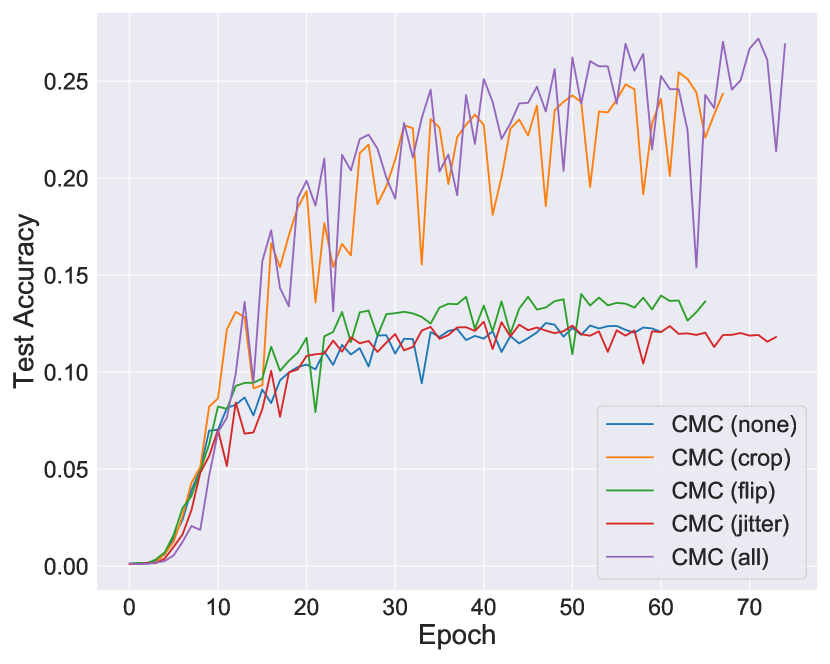
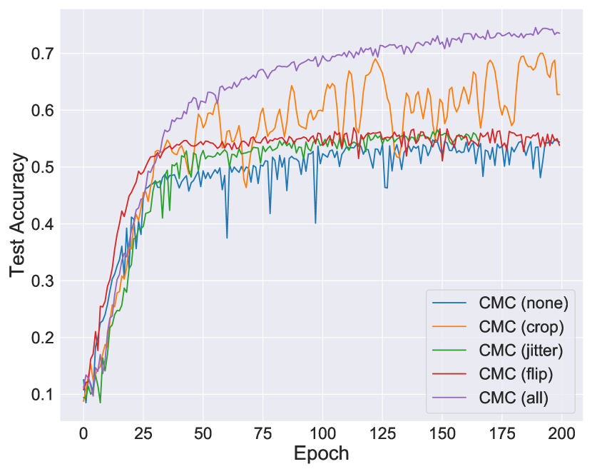
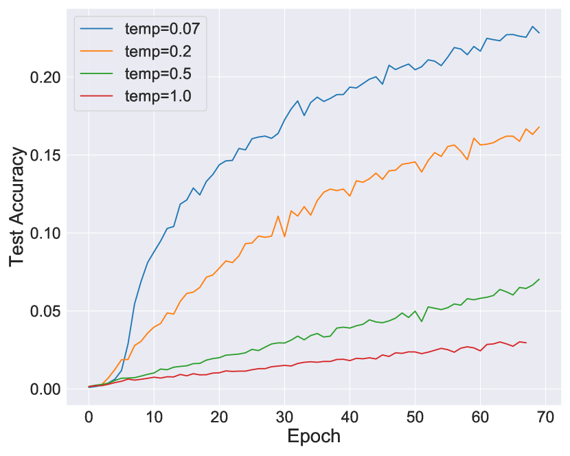
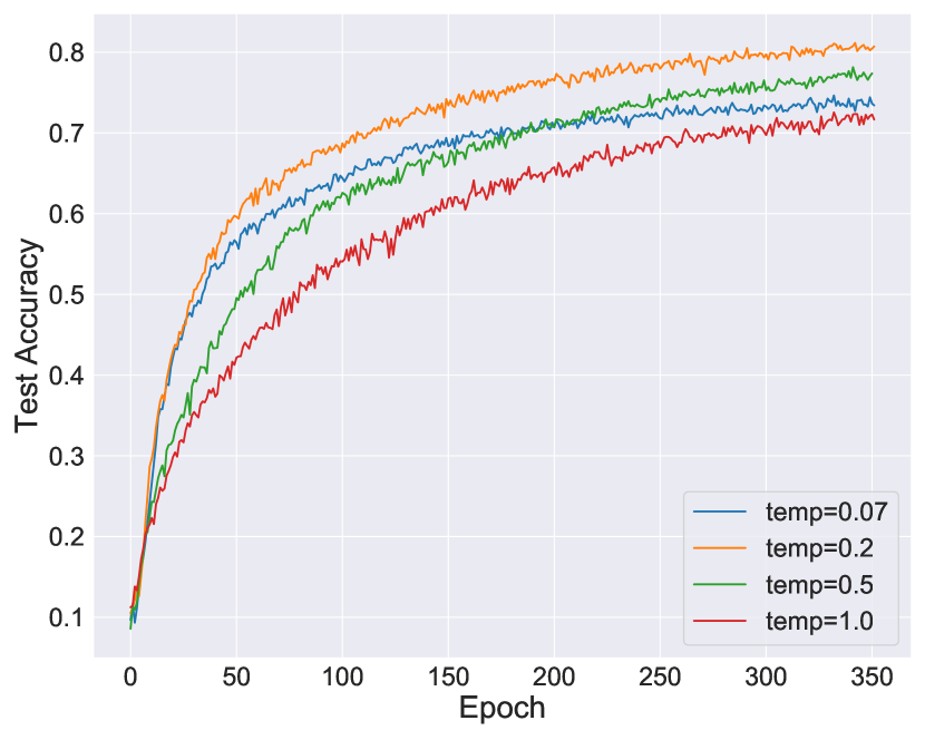
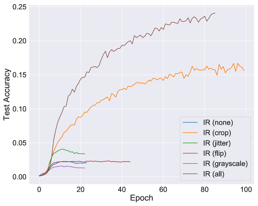
Figure 1: Effect of choice of views on representation quality for IR and CMC on ImageNet. See Fig. 5 for CIFAR10.

Now, succeeding on a transfer task requires the embeddings of data points with similar task labels to be close. While there exists a permutation such that examples of the same class are placed next to each other, there are many others where they are not. It is only with data augmentation that the invariance of Thm. 2.1 is broken: if different data points can yield the same view (a “collision”) then their embeddings cannot be arbitrarily permuted. This implies that augmentation is the crux of learning a good representation. Moreover, not all augmentations are equally good: permutation invariance will be reduced most when the graph of shared views is connected but not dense.

The discussion so far idealizes the embedding functions by ignoring their intrinsic biases: architecture and implicit regularization from SGD may favor certain optima. In the non-idealized setting, IR with no augmentations may already produce non-trivial representations. We turn to experimental evidence to determine the impact of these intrinsic biases compared to those introduce by data augmentation. We train IR and CMC on ImageNet and CIFAR10 with different subsets of augmentations. To measure the quality of the representation, for every image in the test set we predict the label of its closest image in the training set [21].

Fig. 1 clearly shows that without augmentations (the blue line), the representations learned by IR and CMC are significantly worse (though not trivial) than with all augmentations (the brown line). Further, we confirm that not all augmentations lead to good representations: collision-free transformations (e.g. flipping, grayscale) are on par with using no augmentations at all. But, cropping, which certainly introduces collisions, accounts for most of the benefit amongst the basic image augmentations.

Having highlighted the importance of data augmentations, we restate IR to explicitly include them. Define a view function, ν:X×𝒜X:𝜈𝑋𝒜𝑋\nu:X\times\mathcal{A}\rightarrow X that maps the realization of a random variable and an index to another realization. Each index a𝑎a in 𝒜𝒜\mathcal{A} is associated with a composition of augmentations (e.g. cropping plus jitter plus rotation). Assume p(a)𝑝𝑎p(a) is uniform over 𝒜𝒜\mathcal{A}. The IR objective becomes

IR(x(i),M)=𝔼p(a)[logegθ(ν(x(i),a))TM[i]/ωj=1Negθ(ν(x(i),a))TM[j]/ω],superscriptIRsuperscript𝑥𝑖𝑀subscript𝔼𝑝𝑎delimited-[]superscript𝑒subscript𝑔𝜃superscript𝜈superscript𝑥𝑖𝑎𝑇𝑀delimited-[]𝑖𝜔superscriptsubscript𝑗1𝑁superscript𝑒subscript𝑔𝜃superscript𝜈superscript𝑥𝑖𝑎𝑇𝑀delimited-[]𝑗𝜔\scriptstyle\mathcal{L}^{\text{IR}}(x^{(i)},M)=\mathbb{E}_{p(a)}\left[\log\frac{e^{g_{\theta}(\nu(x^{(i)},a))^{T}M[i]/\omega}}{\sum_{j=1}^{N}e^{g_{\theta}(\nu(x^{(i)},a))^{T}M[j]/\omega}}\right],\\ (4)

where the representation M[i]𝑀delimited-[]𝑖M[i] of the i𝑖i-th image x(i)superscript𝑥𝑖x^{(i)} is updated at the m𝑚m-th epoch by the equation M[i]=αM[i]+(1α)gθ(ν(x(i),am)) for amp(a)𝑀delimited-[]𝑖𝛼𝑀delimited-[]𝑖1𝛼subscript𝑔𝜃𝜈superscript𝑥𝑖subscript𝑎𝑚 for subscript𝑎𝑚similar-to𝑝𝑎M[i]=\alpha*M[i]+(1-\alpha)*g_{\theta}(\nu(x^{(i)},a_{m}))\text{ for }a_{m}\sim p(a). We will show that Eq. 4 is equivalent to a bound on mutual information between views, explaining the importance of data augmentations. To do so, we first rehearse a commonly used lower bound on mutual information.

3 Equivalence of Instance Discrimination and Mutual Information

Connections between mutual information and representation learning have been suggested for a family of masked language models [10]. However, the connection has not been deeply explored and a closer look in the visual domain uncovers several insights surrounding contrastive learning.

Mutual information (MI) measures the statistical dependence between two random variables, X𝑋X and Y1subscript𝑌1Y_{1}. In lieu of infeasible integrals, a popular approach is to lower bound MI with InfoNCE [13, 5, 12]:

MI(X;Y1)NCE(X;Y1)=NCE(X;Y1,Y2:K)=𝔼p(x,y1)[fθ,ϕ(x,y1)𝔼p(y2:K)[log1Kj=1Kefθ,ϕ(x,yj)]]MI𝑋subscript𝑌1superscriptNCE𝑋subscript𝑌1superscriptNCE𝑋subscript𝑌1subscript𝑌:2𝐾subscript𝔼𝑝𝑥subscript𝑦1delimited-[]subscript𝑓𝜃italic-ϕ𝑥subscript𝑦1subscript𝔼𝑝subscript𝑦:2𝐾delimited-[]1𝐾superscriptsubscript𝑗1𝐾superscript𝑒subscript𝑓𝜃italic-ϕ𝑥subscript𝑦𝑗\scriptstyle\text{MI}(X;Y_{1})\geq\mathcal{I}^{\textup{NCE}}(X;Y_{1})=\mathcal{I}^{\textup{NCE}}(X;Y_{1},Y_{2:K})=\mathbb{E}_{p(x,y_{1})}\left[f_{\theta,\phi}(x,y_{1})-\mathbb{E}_{p(y_{2:K})}\left[\log\frac{1}{K}\sum_{j=1}^{K}e^{f_{\theta,\phi}(x,y_{j})}\right]\right] (5)

where Y2:Ksubscript𝑌:2𝐾Y_{2:K} are K1𝐾1K-1 independent copies of Y1subscript𝑌1Y_{1}. The witness function fθ,ϕ(x,y)=gθ(x)Tgϕ(y)subscript𝑓𝜃italic-ϕ𝑥𝑦subscript𝑔𝜃superscript𝑥𝑇subscript𝑔italic-ϕ𝑦f_{\theta,\phi}(x,y)=g_{\theta}(x)^{T}g_{\phi}(y) measures the “compatibility” of x𝑥x and y𝑦y. We use gθsubscript𝑔𝜃g_{\theta} and gϕsubscript𝑔italic-ϕg_{\phi} to designate encoders that map realizations of X𝑋X and Yisubscript𝑌𝑖Y_{i} to vectors. The rightmost term in Eq. 5 serves to normalize fθ,ϕ(x,y)subscript𝑓𝜃italic-ϕ𝑥𝑦f_{\theta,\phi}(x,y) with respect to other realizations of Y1subscript𝑌1Y_{1}. We use y2:K={y2,,yK}subscript𝑦:2𝐾subscript𝑦2subscript𝑦𝐾y_{2:K}=\{y_{2},\ldots,y_{K}\} to denote a set of negative samples, or realizations of Y2:Ksubscript𝑌:2𝐾Y_{2:K}. The standard choice for p(y2:K)𝑝subscript𝑦:2𝐾p(y_{2:K}) is i=2Kp(yi)superscriptsubscriptproduct𝑖2𝐾𝑝subscript𝑦𝑖\prod_{i=2}^{K}p(y_{i}). Note we use subscripts i to index values of random variables whereas we used superscripts (i) in Sec. 2 to index a dataset.

In machine learning, we often treat examples from a dataset 𝒟𝒟\mathcal{D} as samples from an empirical distribution p𝒟subscript𝑝𝒟p_{\mathcal{D}}. In Eq. 5, if we replace p(x,y1)𝑝𝑥subscript𝑦1p(x,y_{1}) and p(y2:K)𝑝subscript𝑦:2𝐾p(y_{2:K}) with their empirical analogs, p𝒟(x,y1)subscript𝑝𝒟𝑥subscript𝑦1p_{\mathcal{D}}(x,y_{1}) and p𝒟(y2:K)subscript𝑝𝒟subscript𝑦:2𝐾p_{\mathcal{D}}(y_{2:K}), we call this estimator ^NCE(X;Y1)superscript^NCE𝑋subscript𝑌1\hat{\mathcal{I}}^{\text{NCE}}(X;Y_{1}), or empirical InfoNCE.

3.1 Equivalence of IR and CMC to InfoNCE

To move Eq. 5 toward Eq. 4, consider lower bounding the MI between two weighted view sets with InfoNCE. For views ν:X×2𝒜2X:superscript𝜈𝑋superscript2𝒜superscript2𝑋\nu^{*}:X\times 2^{\mathcal{A}}\rightarrow 2^{X} of index sets A𝒜𝐴𝒜A\subseteq\mathcal{A}, and a set of |A|𝐴|A| weights w𝑤w, define the extended encoder as gθ(v(x,A),w)=xmv(x,A)w[m]gθ(xm)subscriptsuperscript𝑔𝜃superscript𝑣𝑥𝐴𝑤subscriptsubscript𝑥𝑚superscript𝑣𝑥𝐴𝑤delimited-[]𝑚subscript𝑔𝜃subscript𝑥𝑚g^{*}_{\theta}(v^{*}(x,A),w)=\sum_{\begin{subarray}{c}x_{m}\in v^{*}(x,A)\end{subarray}}w[m]\cdot g_{\theta}(x_{m}) where w[m]𝑤delimited-[]𝑚w[m] fetches the m𝑚m-th weight. This encoder leads to the extended witness function fθ(ν(x,A),ν(x,A);w,w)=gθ(ν(x,A),w)Tgθ(ν(x,A),w)/ωsubscriptsuperscript𝑓𝜃superscript𝜈𝑥𝐴superscript𝜈superscript𝑥superscript𝐴𝑤superscript𝑤subscriptsuperscript𝑔𝜃superscriptsuperscript𝜈𝑥𝐴𝑤𝑇subscriptsuperscript𝑔𝜃superscript𝜈superscript𝑥superscript𝐴superscript𝑤𝜔f^{*}_{\theta}(\nu^{*}(x,A),\nu^{*}(x^{\prime},A^{\prime});w,w^{\prime})=g^{*}_{\theta}(\nu^{*}(x,A),w)^{T}g^{*}_{\theta}(\nu^{*}(x^{\prime},A^{\prime}),w^{\prime})/\omega for two realizations x𝑥x, xsuperscript𝑥x^{\prime}. Treating weighted view sets as random variables derived from X𝑋X, we express the InfoNCE bound as

NCE(X;ν)superscriptNCE𝑋superscript𝜈\displaystyle\scriptstyle\mathcal{I}^{\text{NCE}}(X;\nu^{*}) =𝔼A,Ap(A)[NCE(ν(X,A),ν(X,A))]absentsubscript𝔼similar-to𝐴superscript𝐴𝑝𝐴delimited-[]superscriptNCEsuperscript𝜈𝑋𝐴superscript𝜈𝑋superscript𝐴\displaystyle=\scriptstyle\mathbb{E}_{A,A^{\prime}\sim p(A)}\left[\mathcal{I}^{\text{NCE}}(\nu^{*}(X,A),\nu^{*}(X,A^{\prime}))\right] (6)
=𝔼p(x1:K)𝔼A1:K,B,Bp(A)[logefθ(ν(x1,B),ν(x1,B);wB,wB)1Kj=1Kefθ(ν(x1,B),ν(xj,Aj);wB,wAj)].absentsubscript𝔼𝑝subscript𝑥:1𝐾subscript𝔼similar-tosubscript𝐴:1𝐾𝐵superscript𝐵𝑝𝐴delimited-[]superscript𝑒subscriptsuperscript𝑓𝜃superscript𝜈subscript𝑥1𝐵superscript𝜈subscript𝑥1superscript𝐵subscript𝑤𝐵subscript𝑤superscript𝐵1𝐾superscriptsubscript𝑗1𝐾superscript𝑒subscriptsuperscript𝑓𝜃superscript𝜈subscript𝑥1𝐵superscript𝜈subscript𝑥𝑗subscript𝐴𝑗subscript𝑤𝐵subscript𝑤subscript𝐴𝑗\displaystyle=\scriptstyle\mathbb{E}_{p(x_{1:K})}\mathbb{E}_{A_{1:K},B,B^{\prime}\sim p(A)}\left[\log\frac{e^{f^{*}_{\theta}(\nu^{*}(x_{1},B),\nu^{*}(x_{1},B^{\prime});w_{B},w_{B^{\prime}})}}{\frac{1}{K}\sum_{j=1}^{K}e^{f^{*}_{\theta}(\nu^{*}(x_{1},B),\nu^{*}(x_{j},A_{j});w_{B},w_{A_{j}})}}\right]. (7)

Our insight is to characterize the memory bank M𝑀M as a weighted view set. Given the i𝑖i-th image x(i)superscript𝑥𝑖x^{(i)} and M𝑀M with update rate α𝛼\alpha, we estimate the i𝑖i-th entry as M[i]=n=1|𝒜|αn1gθ(ν(x(i),an))m=1nααm1gθ(ν(x(i),am))𝑀delimited-[]𝑖superscriptsubscript𝑛1𝒜superscript𝛼𝑛1subscript𝑔𝜃𝜈superscript𝑥𝑖subscript𝑎𝑛superscriptsubscript𝑚1subscript𝑛𝛼superscript𝛼𝑚1subscript𝑔𝜃𝜈superscript𝑥𝑖subscript𝑎𝑚M[i]=\sum_{n=1}^{|\mathcal{A}|}\alpha^{n-1}g_{\theta}(\nu(x^{(i)},a_{n}))\approx\sum_{m=1}^{n_{\alpha}}\alpha^{m-1}g_{\theta}(\nu(x^{(i)},a_{m})). The left expression enumerates over all elements of the index set 𝒜𝒜\mathcal{A} while the right sums over amp(a)similar-tosubscript𝑎𝑚𝑝𝑎a_{m}\sim p(a), the m𝑚m-th sampled index from 𝒜𝒜\mathcal{A}, over nαsubscript𝑛𝛼n_{\alpha} epochs of training. Because the contribution of any view to the memory bank entry exponentially decays, the first sum is tightly approximated by the second where nαsubscript𝑛𝛼n_{\alpha} is a function of α𝛼\alpha. If α=0𝛼0\alpha=0, then nα=1subscript𝑛𝛼1n_{\alpha}=1.

For each example x(i)superscript𝑥𝑖x^{(i)}, construct two index sets: {a}𝑎\{a\}, the index sampled from p(a)𝑝𝑎p(a) for the current epoch, and A(i)𝒜superscript𝐴𝑖𝒜A^{(i)}\subseteq\mathcal{A}, the indices sampled over the last nαsubscript𝑛𝛼n_{\alpha} epochs of training. Next, fix weights w1={1}subscript𝑤11w_{1}=\{1\} and w2={1,α,,αnα1}subscript𝑤21𝛼superscript𝛼subscript𝑛𝛼1w_{2}=\{1,\alpha,\ldots,\alpha^{{n_{\alpha}}-1}\}. Consider the special case of Eq. 7 where the witness function is fθ(ν(x(i),{a}),ν(x(i),A(i));w1,w2)subscriptsuperscript𝑓𝜃superscript𝜈superscript𝑥𝑖𝑎superscript𝜈superscript𝑥𝑖superscript𝐴𝑖subscript𝑤1subscript𝑤2f^{*}_{\theta}(\nu^{*}(x^{(i)},\{a\}),\nu^{*}(x^{(i)},A^{(i)});w_{1},w_{2}), the weighted dot product between the current view of x(i)superscript𝑥𝑖x^{(i)} and the stored representation from the bank. The next lemma shows that this special case of InfoNCE is equivalent to IR and CMC. The proof can be found in Sec. A.2.

Lemma 3.1.

Let p𝒟(x)subscript𝑝𝒟𝑥p_{\mathcal{D}}(x) be an empirical distribution over images x𝑥x, 𝒟𝒟\mathcal{D} a dataset whose members are sampled i.i.d. from p𝒟subscript𝑝𝒟p_{\mathcal{D}}, and M𝑀M a memory bank. Let 𝒜IRsubscript𝒜IR\mathcal{A}_{\textup{IR}} and 𝒜CMCsubscript𝒜CMC\mathcal{A}_{\textup{CMC}} be two sets of indices where each index is associated with an image augmentation in IR and an image augmentation in CMC, respectively. Now, define two extended view functions, νIR:X×2𝒜IR2X:subscriptsuperscript𝜈IR𝑋superscript2subscript𝒜IRsuperscript2𝑋\nu^{*}_{\textup{IR}}:X\times 2^{\mathcal{A}_{\textup{IR}}}\rightarrow 2^{X} and νCMC:X×2𝒜CMC2X:subscriptsuperscript𝜈CMC𝑋superscript2subscript𝒜CMCsuperscript2𝑋\nu^{*}_{\textup{CMC}}:X\times 2^{\mathcal{A}_{\textup{CMC}}}\rightarrow 2^{X}. If we use K𝐾K negative samples, then ^NCE(X;νIR)𝔼p𝒟[IR(x,M)]+logKκsuperscript^NCE𝑋subscriptsuperscript𝜈IRsubscript𝔼subscript𝑝𝒟delimited-[]superscriptIR𝑥𝑀𝐾𝜅\hat{\mathcal{I}}^{\textup{NCE}}(X;\nu^{*}_{\textup{IR}})\equiv\mathbb{E}_{p_{\mathcal{D}}}\left[\mathcal{L}^{\textup{IR}}(x,M)\right]+\log\frac{K}{\kappa}, and ^NCE(X;νCMC)𝔼p𝒟[CMC(x,M)]/2+logKκsuperscript^NCE𝑋subscriptsuperscript𝜈CMCsubscript𝔼subscript𝑝𝒟delimited-[]superscriptCMC𝑥𝑀2𝐾𝜅\hat{\mathcal{I}}^{\textup{NCE}}(X;\nu^{*}_{\textup{CMC}})\equiv\mathbb{E}_{p_{\mathcal{D}}}\left[\mathcal{L}^{\textup{CMC}}(x,M)\right]/2+\log\frac{K}{\kappa} where the symbol \equiv implies equivalence.

Lemma 3.1 provides insight into IR and CMC: the objectives both lower bound MI but using different view sets. As L and ab capture nearly disjoint information, CMC imposes a strong information bottleneck between any two views. Thus, we see why in Fig. 1, CMC maintains a higher performance without any augmentations compared to IR: the view set for CMC is always nontrivial.

3.2 Simplifying Instance Discrimination

The equivalence to mutual information can help us pick hyperparameters and simplify IR.

Refer to caption
(a) Stability (\dagger)
Refer to caption
(b) Stability (\ddagger)
Refer to caption
(c) α𝛼\alpha+IR (\dagger)
Refer to caption
(d) α𝛼\alpha+LA (\dagger)
Refer to caption
(e) α𝛼\alpha+IR (\ddagger)
Refer to caption
(f) α𝛼\alpha+CMC (\ddagger)
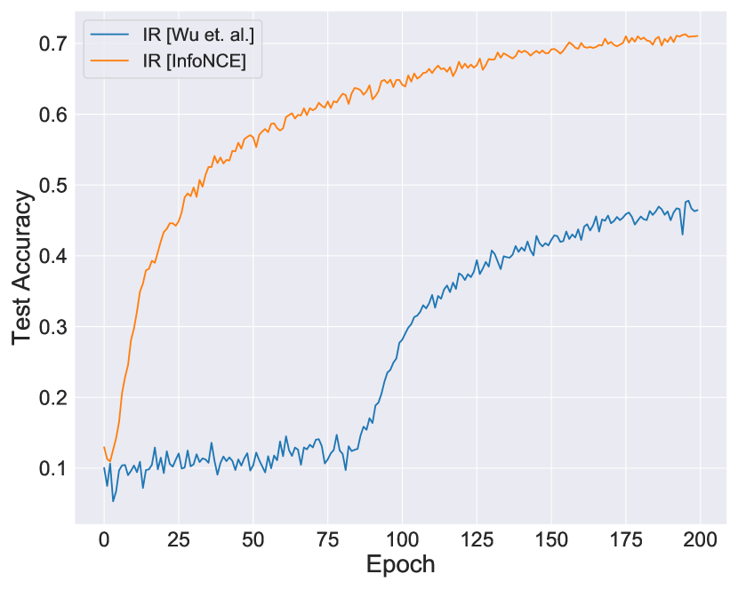
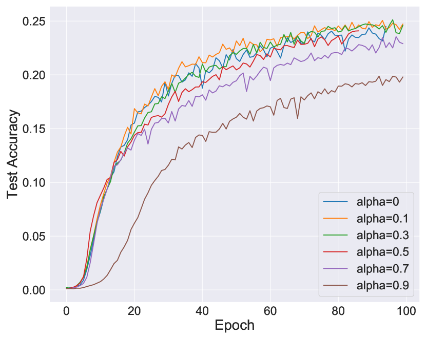
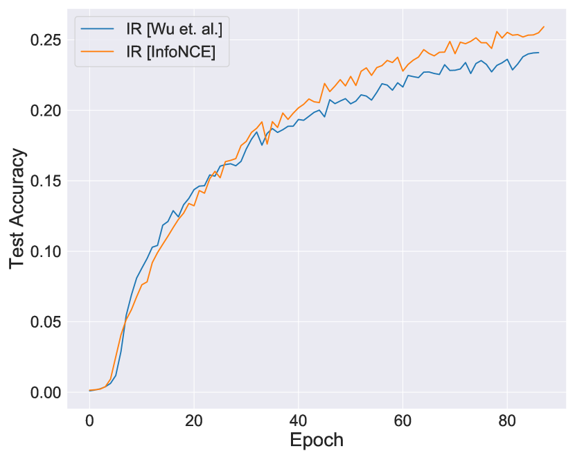
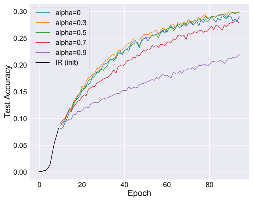
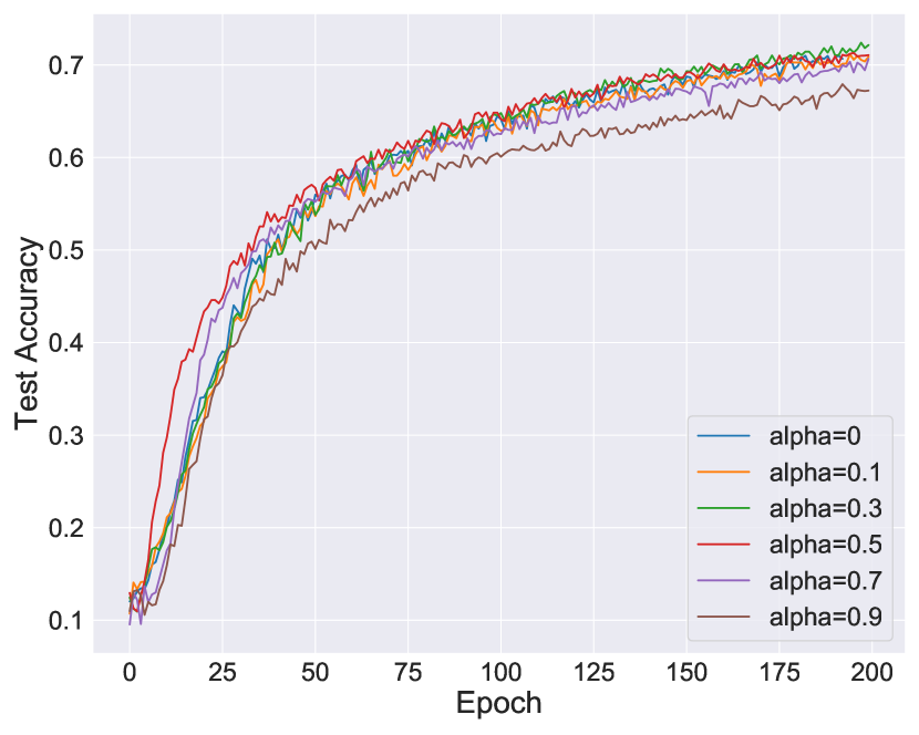
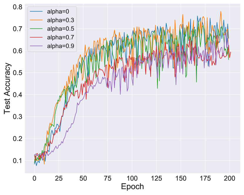
Figure 2: Nearest neighbor classification accuracy comparing IR with InfoNCE in stability (a,b), and different α𝛼\alpha for the memory bank of IR, LA (e-h) on Imagenet (\dagger) and CIFAR10 (\ddagger).

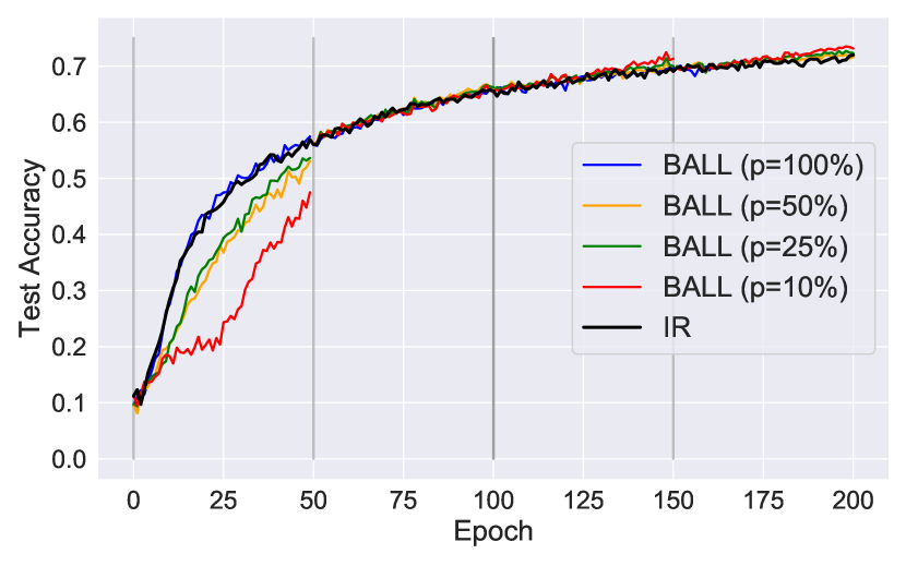
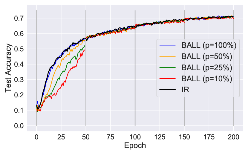
Softmax “hacks” are unnecessary.    The original IR implementation used several innovations to make a million-category classification problem tractable. For instance, IR approximates the denominator in Eq. 1 with K𝐾K samples scaled by κ=2876934.21281167𝜅2876934.21281167\kappa=\frac{2876934.2}{1281167}. Such practices were propagated to LA and CMC in their official implementations. While this works well for ImageNet, it is not clear how to set the constant for other datasets. For small datasets like CIFAR10, such large constants introduce numerical instability in themselves. However, once we draw the relation between IR and MI, we immediately see that there is no need to compute the softmax (and no need for κ𝜅\kappa); InfoNCE only requires a logsumexp over the K𝐾K samples, a much more stable operation. Fig. 2c and d show the effect of switching from the original IR code to InfoNCE. While we expected to find the large impact in CIFAR10, we also find that in ImageNet (for which the constants were tuned) our simplification improves performance. Later, we refer to this “simplified IR”, as IRncence{}^{\text{nce}}.

The memory bank is not critical.    The memory bank makes Eq. 7 quite involved. Yet the MI between weighted views should be very similar to the average MI between the underlying views. We thus consider the special case when α=0𝛼0\alpha=0. Here, the i𝑖i-th entry M[i]𝑀delimited-[]𝑖M[i] stores only the encoding of a single view chosen in the last epoch. As such, we can simplify and remove the memory bank altogether. We compare these formulations experimentally by nearest neighbor classification. Fig. 2e-g show results varying α𝛼\alpha from 0 (no memory bank) to near 1 (a very slowly updated bank). We find performance when α=0𝛼0\alpha=0 and when α=0.5𝛼0.5\alpha=0.5 (the standard approach) is equal across algorithms and datasets. This suggests that we can replace M𝑀M with two random views every iteration. SimCLR [1] has suggested a similar finding – and the MI framework makes such a simplification natural. With this formulation, we show SimCLR is equivalent to InfoNCE as well (see lemma B.1). In the experiments below we keep the memory bank to make comparison to previous work easier.

4 Equivalence of Local Aggregation and Mutual Information

Having shown an equivalence between IR, CMC, SimCLR, and InfoNCE, we might wish to do the same for LA. However, the close and background neighbor sets of LA are not obviously related to MI. To uncover the relation, we generalize InfoNCE to support sampling from a variational distribution.

4.1 A Variational Lower Bound on Mutual Information

Recall that InfoNCE draws negative samples independently from p(y)𝑝𝑦p(y). However, we may wish to choose negative samples from a different distribution over sets q(y2:K)𝑞subscript𝑦:2𝐾q(y_{2:K}) or even conditionally sample negatives, q(y2:K|y1)𝑞conditionalsubscript𝑦:2𝐾subscript𝑦1q(y_{2:K}|y_{1}) where y1p(y)similar-tosubscript𝑦1𝑝𝑦y_{1}\sim p(y). While previous literature presents InfoNCE with an arbitrary distribution [12, 10] that would justify either of these choices, we have not found a proof supporting this. One of our contributions is to formally define a class of variational distributions q(y2:K|y1)𝑞conditionalsubscript𝑦:2𝐾subscript𝑦1q(y_{2:K}|y_{1}) such that Eq. 5 remains a valid lower bound if we replace p(y2:K)𝑝subscript𝑦:2𝐾p(y_{2:K}) with q(y2:K|y1)𝑞conditionalsubscript𝑦:2𝐾subscript𝑦1q(y_{2:K}|y_{1}):

Theorem 4.1.

Fix a distribution \mathbb{P} over (d,d)superscript𝑑subscriptsuperscript𝑑(\mathbb{R}^{d},\mathcal{B}_{\mathbb{R}^{d}}). Fix any xdsuperscript𝑥superscript𝑑x^{*}\in\mathbb{R}^{d} and any f:d×d:𝑓superscript𝑑superscript𝑑f:\mathbb{R}^{d}\times\mathbb{R}^{d}\rightarrow\mathbb{R}. Define g(x)=ef(x,x)𝑔𝑥superscript𝑒𝑓superscript𝑥𝑥g(x)=e^{f(x^{*},x)} and suppose that g𝑔g is \mathbb{P}-integrable with mean c𝑐c. Pick a set T𝑇T\subset\mathbb{R} lower-bounded by some τ>logc𝜏𝑐\tau>\log c in ¯¯\overline{\mathbb{R}} and define ST={x|f(x,x)T}subscript𝑆𝑇conditional-set𝑥𝑓superscript𝑥𝑥𝑇S_{T}=\{x|f(x^{*},x)\in T\} to be the pre-image under f(x,)𝑓superscript𝑥f(x^{*},\cdot) of T𝑇T; suppose that (ST)>0subscript𝑆𝑇0\mathbb{P}(S_{T})>0. Define T(A)=(A|ST)subscript𝑇𝐴conditional𝐴subscript𝑆𝑇\mathbb{Q}_{T}(A)=\mathbb{P}(A|S_{T}) for any Borel A𝐴A. Then 𝔼[g(x)]<𝔼T[g(x)]subscript𝔼delimited-[]𝑔𝑥subscript𝔼subscript𝑇delimited-[]𝑔𝑥\mathbb{E}_{\mathbb{P}}[g(x)]<\mathbb{E}_{\mathbb{Q}_{T}}[g(x)].

Next, we define the variational InfoNCE, or VINCE, estimator and use Thm. 4.1 to show that it lower-bounds InfoNCE, and thus mutual information.

Corollary 4.1.1.

Fix X𝑋X and Y1,,YKsubscript𝑌1subscript𝑌𝐾Y_{1},...,Y_{K}, the latter i.i.d. according to a distribution p𝑝p. Suppose we sample x,y1p(x,y1)similar-to𝑥subscript𝑦1𝑝𝑥subscript𝑦1x,y_{1}\sim p(x,y_{1}). For f:(Yi,Yj):𝑓subscript𝑌𝑖subscript𝑌𝑗f:(Y_{i},Y_{j})\rightarrow\mathbb{R} define ST={y|τf(y1,y)T}subscript𝑆𝑇conditional-set𝑦𝜏𝑓subscript𝑦1𝑦𝑇S_{T}=\{y|\tau\leq f(y_{1},y)\in T\} with τ>log𝔼p(y)[ef(y1,y)]𝜏subscript𝔼𝑝𝑦delimited-[]superscript𝑒𝑓subscript𝑦1𝑦\tau>\log\mathbb{E}_{p(y)}[e^{f(y_{1},y)}] and T𝑇T lower bounded by τ𝜏\tau. For any Borel A=A2×.×AKA=A_{2}\times....\times A_{K}, define a distribution over Y2:K=(Y2,,YK)subscript𝑌:2𝐾subscript𝑌2subscript𝑌𝐾Y_{2:K}=(Y_{2},...,Y_{K}) by qT(Y2:KA)=j=2Kp(Aj|ST)subscript𝑞𝑇subscript𝑌:2𝐾𝐴superscriptsubscriptproduct𝑗2𝐾𝑝conditionalsubscript𝐴𝑗subscript𝑆𝑇q_{T}(Y_{2:K}\in A)=\prod_{j=2}^{K}p(A_{j}|S_{T}). If we let VINCE(X;Y1)=𝔼p(x,y1)𝔼y2:KqT[logef(x,y1)1Kj=1Kef(x,yj)]superscriptVINCE𝑋subscript𝑌1subscript𝔼𝑝𝑥subscript𝑦1subscript𝔼similar-tosubscript𝑦:2𝐾subscript𝑞𝑇delimited-[]superscript𝑒𝑓𝑥subscript𝑦11𝐾superscriptsubscript𝑗1𝐾superscript𝑒𝑓𝑥subscript𝑦𝑗\mathcal{I}^{\text{VINCE}}(X;Y_{1})=\mathbb{E}_{p(x,y_{1})}\mathbb{E}_{y_{2:K}\sim q_{T}}\left[\log\frac{e^{f(x,y_{1})}}{\frac{1}{K}\sum_{j=1}^{K}e^{f(x,y_{j})}}\right], then VINCENCEsuperscriptVINCEsuperscriptNCE\mathcal{I}^{\text{VINCE}}\leq\mathcal{I}^{\text{NCE}}.

With Coro. 4.1.1, we are equipped to formalize the connection between LA and information.

4.2 Equivalence of LA and VINCE

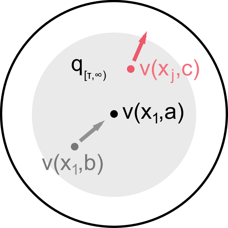
Focusing first on the background neighborhood, consider sampling from q[τ,)(x|ν(x1,a))subscript𝑞𝜏conditional𝑥𝜈subscript𝑥1𝑎q_{[\tau,\infty)}(x|\nu(x_{1},a)) as defined in Thm 4.1 with x1subscript𝑥1x_{1} being the current image and a𝑎a the current index in 𝒜𝒜\mathcal{A}. A larger threshold τ𝜏\tau chooses negatives that more closely resemble gθ(ν(x1,a))subscript𝑔𝜃𝜈subscript𝑥1𝑎g_{\theta}(\nu(x_{1},a)), the representation of the current view of x1subscript𝑥1x_{1}. This poses a more challenging problem: encoders must now distinguish between more similar objects, forcing the representation to be more semantically meaningful. Replacing p(x1)𝑝subscript𝑥1p(x_{1}) with q[τ,)(x|ν(x1,a))subscript𝑞𝜏conditional𝑥𝜈subscript𝑥1𝑎q_{[\tau,\infty)}(x|\nu(x_{1},a)) immediately suggests a new algorithm that “interpolates” between IR and LA.

Lemma 4.2.

Let X1subscript𝑋1X_{1} be a random variable and X2:Ksubscript𝑋:2𝐾X_{2:K} be i.i.d. copies. Let 𝒟𝒟\mathcal{D} be a dataset of realizations of X1subscript𝑋1X_{1} sampled from an empirical distribution p𝒟subscript𝑝𝒟p_{\mathcal{D}}. Fix a realization x1𝒟subscript𝑥1𝒟x_{1}\in\mathcal{D}, an index a𝒜𝑎𝒜a\in\mathcal{A}, and a view function ν𝜈\nu. Assuming τ>log𝔼xp(x)[efθ(ν(x1,a),x)]𝜏subscript𝔼similar-to𝑥𝑝𝑥delimited-[]superscript𝑒subscript𝑓𝜃𝜈subscript𝑥1𝑎𝑥\tau>\log\mathbb{E}_{x\sim p(x)}\left[e^{f_{\theta}(\nu(x_{1},a),x)}\right], we define qT(x2:K|ν(x1,a))=j=2KqT(xj|ν(x1,a))subscript𝑞𝑇conditionalsubscript𝑥:2𝐾𝜈subscript𝑥1𝑎superscriptsubscriptproduct𝑗2𝐾subscript𝑞𝑇conditionalsubscript𝑥𝑗𝜈subscript𝑥1𝑎q_{T}(x_{2:K}|\nu(x_{1},a))=\prod_{j=2}^{K}q_{T}(x_{j}|\nu(x_{1},a)) for any set T𝑇T lower bounded by τ𝜏\tau, from which we draw realizations of X2:Ksubscript𝑋:2𝐾X_{2:K}. Assume xj𝒟subscript𝑥𝑗𝒟x_{j}\in\mathcal{D} for j[K]𝑗delimited-[]𝐾j\in[K] and let ρ(xj)𝜌subscript𝑥𝑗\rho(x_{j}) return the index of xjsubscript𝑥𝑗x_{j} in 𝒟𝒟\mathcal{D}. For any T𝑇T, we define T(x1,M)=𝔼p(a)𝔼qT(x2:K|ν(x1,a))[logegθ(ν(x1,a))TM[ρ(x1)]/ωj=1Kegθ(ν(x1,a))TM[ρ(xj)]/ω]superscript𝑇subscript𝑥1𝑀subscript𝔼𝑝𝑎subscript𝔼subscript𝑞𝑇conditionalsubscript𝑥:2𝐾𝜈subscript𝑥1𝑎delimited-[]superscript𝑒subscript𝑔𝜃superscript𝜈subscript𝑥1𝑎𝑇𝑀delimited-[]𝜌subscript𝑥1𝜔superscriptsubscript𝑗1𝐾superscript𝑒subscript𝑔𝜃superscript𝜈subscript𝑥1𝑎𝑇𝑀delimited-[]𝜌subscript𝑥𝑗𝜔\scriptstyle\mathcal{L}^{T}(x_{1},M)=\mathbb{E}_{p(a)}\mathbb{E}_{q_{T}(x_{2:K}|\nu(x_{1},a))}\left[\log\frac{e^{g_{\theta}(\nu(x_{1},a))^{T}M[\rho(x_{1})]/\omega}}{\sum_{j=1}^{K}e^{g_{\theta}(\nu(x_{1},a))^{T}M[\rho(x_{j})]/\omega}}\right]. Then ^VINCE(X1;ν)𝔼p𝒟(x)[T(x,M)]+logKsuperscript^VINCEsubscript𝑋1superscript𝜈subscript𝔼subscript𝑝𝒟𝑥delimited-[]superscript𝑇𝑥𝑀𝐾\hat{\mathcal{I}}^{\textup{VINCE}}(X_{1};\nu^{*})\equiv\mathbb{E}_{p_{\mathcal{D}}(x)}[\mathcal{L}^{T}(x,M)]+\log K. In particular, we call BALL(x1,M)=[τ,)(x1,M)superscriptBALLsubscript𝑥1𝑀superscript𝜏subscript𝑥1𝑀\mathcal{L}^{\textup{BALL}}(x_{1},M)=\mathcal{L}^{[\tau,\infty)}(x_{1},M), Ball Discrimination (BALL).

The primary distinction of BALL from IR is that negative samples are drawn from a restricted domain. Thus, we cannot equate the BALL estimator to InfoNCE; we must rely on VINCE, which provides the machinery to use a conditional distribution with smaller support. We will use BALL to show that LA lower bounds MI between weighted view sets. To do so, consider a simplified version of LA where we assume that the close neighbor set contains only the current image. That is, C(ρ(x1))={ρ(x1)}superscript𝐶𝜌subscript𝑥1𝜌subscript𝑥1C^{(\rho(x_{1}))}=\{\rho(x_{1})\} in the notation of Sec. 2. We call this LA0. We show that LA0 is equivalent to BALL.

Lemma 4.3.

Fix xp𝒟(x)similar-to𝑥subscript𝑝𝒟𝑥x\sim p_{\mathcal{D}}(x) and C(ρ(x))={ρ(x)}superscript𝐶𝜌𝑥𝜌𝑥C^{(\rho(x))}=\{\rho(x)\}. Then LA0(x,M)=BALL(x,M)superscriptsubscriptLA0𝑥𝑀superscriptBALL𝑥𝑀\mathcal{L}^{\textup{LA}_{0}}(x,M)=\mathcal{L}^{\textup{BALL}}(x,M).

Now, the numerator of the LA0 objective contains a term egθ(ν(x(i),a))TM[i]superscript𝑒subscript𝑔𝜃superscript𝜈superscript𝑥𝑖𝑎𝑇𝑀delimited-[]𝑖e^{g_{\theta}(\nu(x^{(i)},a))^{T}M[i]} whereas the numerator of the more general LA is kC(i)egθ(ν(x(i),a))TM[k]subscript𝑘superscript𝐶𝑖superscript𝑒subscript𝑔𝜃superscript𝜈superscript𝑥𝑖𝑎𝑇𝑀delimited-[]𝑘\sum_{k\in C^{(i)}}e^{g_{\theta}(\nu(x^{(i)},a))^{T}M[k]}. Note that the dot product between embeddings of any two views of x(i)superscript𝑥𝑖x^{(i)} must be at least as large as the dot product between embeddings of a view of x(i)superscript𝑥𝑖x^{(i)} and a view of x(j)superscript𝑥𝑗x^{(j)}, with equality if and only if views collide. Since |C(i)|egθ(ν(x(i),a))TM[i]kC(i)egθ(ν(x(i),a))TM[k]superscript𝐶𝑖superscript𝑒subscript𝑔𝜃superscript𝜈superscript𝑥𝑖𝑎𝑇𝑀delimited-[]𝑖subscript𝑘superscript𝐶𝑖superscript𝑒subscript𝑔𝜃superscript𝜈superscript𝑥𝑖𝑎𝑇𝑀delimited-[]𝑘|C^{(i)}|e^{g_{\theta}(\nu(x^{(i)},a))^{T}M[i]}\geq\sum_{k\in C^{(i)}}e^{g_{\theta}(\nu(x^{(i)},a))^{T}M[k]}, we can bound LA by LA0 subject to an additive constant.

Lemma 4.4.

Fix xp𝒟(x)similar-to𝑥subscript𝑝𝒟𝑥x\sim p_{\mathcal{D}}(x) and ρ(x)C(ρ(x))𝜌𝑥superscript𝐶𝜌𝑥\rho(x)\in C^{(\rho(x))}. Then LA0(x,M)LA(x,M)log|C(ρ(x))|superscriptsubscriptLA0𝑥𝑀superscriptLA𝑥𝑀superscript𝐶𝜌𝑥\mathcal{L}^{\textup{LA}_{0}}(x,M)\geq\mathcal{L}^{\textup{LA}}(x,M)-\log|C^{(\rho(x))}|.

As LA is bounded by BALL, it is bounded by VINCE and thus MI as well.

We end with an observation about LA. The overall objective for BALL includes an expectation over view pairs. An elegant way to understand “close neighbors” in LA is as an extension to this view distribution: treat the views of all elements from C(i)superscript𝐶𝑖C^{(i)} as views of x(i)superscript𝑥𝑖x^{(i)}. The actual LA objective makes one additional change, applying Jensen’s inequality to move the sum over close neighbors inside the log, yielding a tighter bound on BALL:

𝔼p(a)𝔼q[τ,)[log1|C|lCegθ(ν(x1,a))TM[l]j=1Kegθ(ν(x1,a))TM[ρ(xj)]]𝔼p(a)𝔼q[τ,)𝔼qC[l{ρ(xl)}logegθ(ν(x1,a))TM[l]j=1Kegθ(ν(x1,a))TM[ρ(xj)]]subscript𝔼𝑝𝑎subscript𝔼subscript𝑞𝜏delimited-[]1𝐶subscript𝑙𝐶superscript𝑒subscript𝑔𝜃superscript𝜈subscript𝑥1𝑎𝑇𝑀delimited-[]𝑙superscriptsubscript𝑗1𝐾superscript𝑒subscript𝑔𝜃superscript𝜈subscript𝑥1𝑎𝑇𝑀delimited-[]𝜌subscript𝑥𝑗subscript𝔼𝑝𝑎subscript𝔼subscript𝑞𝜏subscript𝔼subscript𝑞𝐶delimited-[]subscript𝑙𝜌subscriptsuperscript𝑥𝑙superscript𝑒subscript𝑔𝜃superscript𝜈subscript𝑥1𝑎𝑇𝑀delimited-[]𝑙superscriptsubscript𝑗1𝐾superscript𝑒subscript𝑔𝜃superscript𝜈subscript𝑥1𝑎𝑇𝑀delimited-[]𝜌subscript𝑥𝑗\displaystyle\scriptstyle\mathbb{E}_{p(a)}\mathbb{E}_{q_{[\tau,\infty)}}\left[\log\frac{\frac{1}{|C|}\sum_{l\in C}e^{g_{\theta}(\nu(x_{1},a))^{T}M[l]}}{\sum_{j=1}^{K}e^{g_{\theta}(\nu(x_{1},a))^{T}M[\rho(x_{j})]}}\right]\scriptstyle\geq\mathbb{E}_{p(a)}\mathbb{E}_{q_{[\tau,\infty)}}\mathbb{E}_{q_{C}}\left[\sum_{l\in\{\rho({x^{\prime}_{l}})\}}\log\frac{e^{g_{\theta}(\nu(x_{1},a))^{T}M[l]}}{\sum_{j=1}^{K}e^{g_{\theta}(\nu(x_{1},a))^{T}M[\rho(x_{j})]}}\right]

where x2:Kq[τ,)similar-tosubscript𝑥:2𝐾subscript𝑞𝜏x_{2:K}\sim q_{[\tau,\infty)}, qCsubscript𝑞𝐶q_{C} is uniform over close neighbors (to the current view), and x2:LqCsimilar-tosubscriptsuperscript𝑥:2𝐿subscript𝑞𝐶x^{\prime}_{2:L}\sim q_{C}. The left expression is LA(x1,M)superscriptLAsubscript𝑥1𝑀\mathcal{L}^{\textup{LA}}(x_{1},M) and the right expression is the objective that extends the view set.

4.3 Simplifying and Generalizing Local Aggregation

As in Sec. 3.2, we can simplify LA after formulating it as mutual information. In particular, these insights lead to new variants of Ball Discrimination and Local Aggregation.

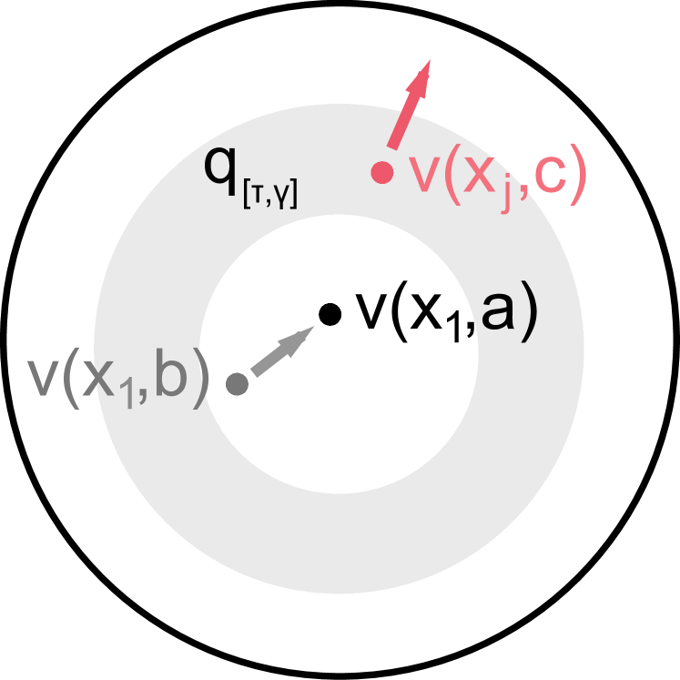
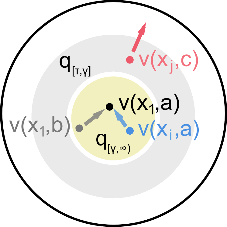
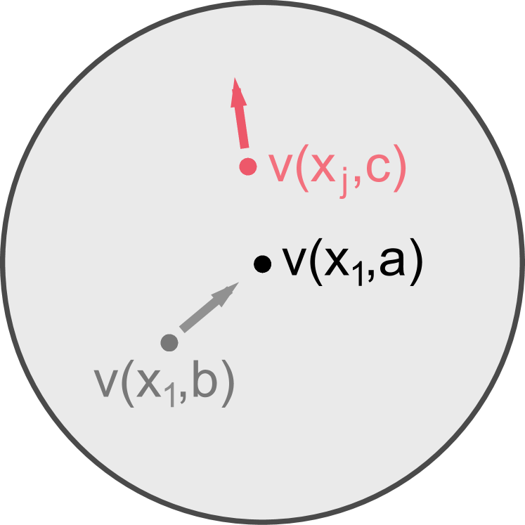
Ring and Cave Discrimination. We consider two extensions of BALL, where the negative samples are picked from a ball centered around gθ(ν(x1,a))subscript𝑔𝜃𝜈subscript𝑥1𝑎g_{\theta}(\nu(x_{1},a)) for some a𝑎a. Like LA, we might fear that the elements very close to x1subscript𝑥1x_{1} in the ball would serve as poor negative examples. However, LA treats these elements as both close neighbors and negatives, which seems contradictory. Instead, we propose two ways to cut out a region in the ball of negative samples. First, take a smaller ball with the same center. Define Ring Discrimination (RING) as RING(x1,M)=𝔼p(a)𝔼q[τ,γ](x2:K|ν(x1,a))[logegθ(ν(x1,a))TM[ρ(x1)]/ωj=1Kegθ(ν(x1,a))TM[ρ(xj)]/ω]superscriptRINGsubscript𝑥1𝑀subscript𝔼𝑝𝑎subscript𝔼subscript𝑞𝜏𝛾conditionalsubscript𝑥:2𝐾𝜈subscript𝑥1𝑎delimited-[]superscript𝑒subscript𝑔𝜃superscript𝜈subscript𝑥1𝑎𝑇𝑀delimited-[]𝜌subscript𝑥1𝜔superscriptsubscript𝑗1𝐾superscript𝑒subscript𝑔𝜃superscript𝜈subscript𝑥1𝑎𝑇𝑀delimited-[]𝜌subscript𝑥𝑗𝜔\mathcal{L}^{\textup{RING}}(x_{1},M)=\mathbb{E}_{p(a)}\mathbb{E}_{q_{[\tau,\gamma]}(x_{2:K}|\nu(x_{1},a))}\left[\log\frac{e^{g_{\theta}(\nu(x_{1},a))^{T}M[\rho(x_{1})]/\omega}}{\sum_{j=1}^{K}e^{g_{\theta}(\nu(x_{1},a))^{T}M[\rho(x_{j})]/\omega}}\right]. That is, RING samples negatives from a distribution q[τ,γ]subscript𝑞𝜏𝛾q_{[\tau,\gamma]} over a ring formed by the difference between the two balls.

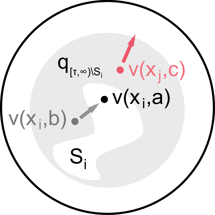
Next, like LA, consider running K-means on samples, x1p𝒟(x)similar-tosubscript𝑥1subscript𝑝𝒟𝑥x_{1}\sim p_{\mathcal{D}}(x) and x2:Kq[τ,)similar-tosubscript𝑥:2𝐾subscript𝑞𝜏x_{2:K}\sim q_{[\tau,\infty)} (the outer ball). Let S1subscript𝑆1S_{1} contain elements with the same cluster assignment as x1subscript𝑥1x_{1}. Define CAVE Discrimination (CAVE) as CAVE(x1,M)=𝔼p(a)𝔼q[τ,)S1(x2:K|ν(x1,a))[logegθ(ν(x1,a))TM[ρ(x1)]/ωj=1Kegθ(ν(x1,a))TM[ρ(xj)]/ω]superscriptCAVEsubscript𝑥1𝑀subscript𝔼𝑝𝑎subscript𝔼subscript𝑞𝜏subscript𝑆1conditionalsubscript𝑥:2𝐾𝜈subscript𝑥1𝑎delimited-[]superscript𝑒subscript𝑔𝜃superscript𝜈subscript𝑥1𝑎𝑇𝑀delimited-[]𝜌subscript𝑥1𝜔superscriptsubscript𝑗1𝐾superscript𝑒subscript𝑔𝜃superscript𝜈subscript𝑥1𝑎𝑇𝑀delimited-[]𝜌subscript𝑥𝑗𝜔\mathcal{L}^{\textup{CAVE}}(x_{1},M)=\mathbb{E}_{p(a)}\mathbb{E}_{q_{[\tau,\infty)\setminus S_{1}}(x_{2:K}|\nu(x_{1},a))}\left[\log\frac{e^{g_{\theta}(\nu(x_{1},a))^{T}M[\rho(x_{1})]/\omega}}{\sum_{j=1}^{K}e^{g_{\theta}(\nu(x_{1},a))^{T}M[\rho(x_{j})]/\omega}}\right]. That is, CAVE samples negatives from a distribution q[τ,)S1subscript𝑞𝜏subscript𝑆1q_{[\tau,\infty)\setminus S_{1}} over the outer ball subtracting a set. Lemma B.2 show RING and CAVE lower bound MI between weighted view sets.
Refer to caption
(a) IR
Refer to caption
(b) BALL
Refer to caption
(c) RING
Refer to caption
(d) CAVE
Refer to caption
(e) LA
Refer to caption
(f) RINGs-neighs-neigh{}^{\text{s-neigh}}
Refer to caption
(g) BALLannealanneal{}^{\text{anneal}}
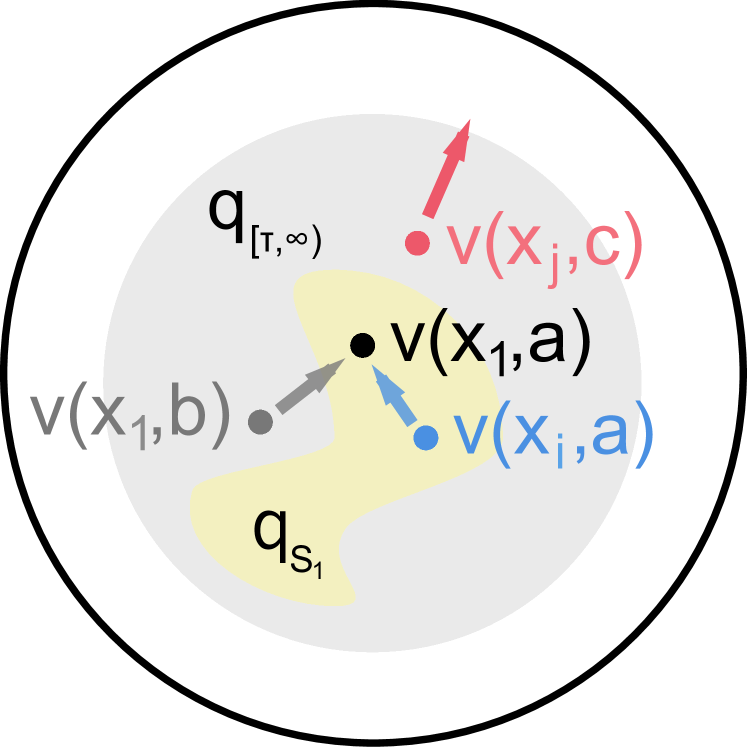
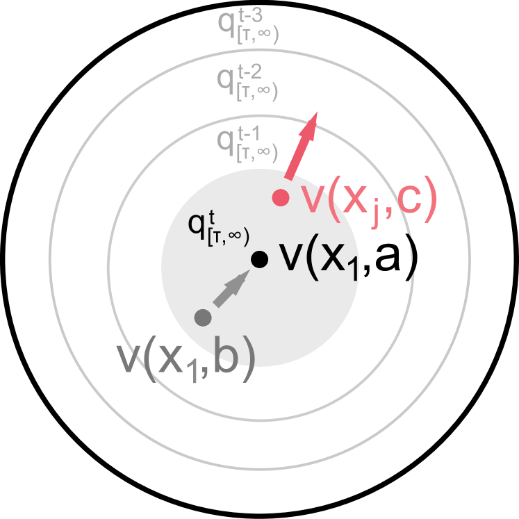
Figure 3: Various contrastive algorithms. Black: current view of image x1subscript𝑥1x_{1}; gray: other views of x1subscript𝑥1x_{1}; red: negative samples; gray: negative distribution; yellow: neighbor distribution.

K-Neighbor and S-Neighbor views. We hypothesize that one of the strengths of LA is optimizing representations to put close neighbors near each other. Naturally, we similarly extend BALL, RING, and CAVE to push close neighbors together. In addition to the VINCE distribution qTsubscript𝑞𝑇q_{T} used for negative sampling (e.g. T=[τ,γ]𝑇𝜏𝛾T=[\tau,\gamma] for RING), define a second VINCE distribution qCsubscript𝑞𝐶q_{C} with set C𝐶C lower bounded by τ𝜏\tau to sample “close neighbors”. We explore two possible choices for qCsubscript𝑞𝐶q_{C}. Fix x1subscript𝑥1x_{1} as some example from our dataset. First, by S-neighborhood, we set C=[γ,)𝐶𝛾C=[\gamma,\infty), the inner ball defined by RING. Second, by K-neighborhood, we set C=S1𝐶subscript𝑆1C=S_{1}, the set of elements with the same cluster assignment as x1subscript𝑥1x_{1} given by K-means. In our experiments, we denote each with a superscript s-neighs-neigh{}^{\text{s-neigh}} or k-neighk-neigh{}^{\text{k-neigh}} with no superscript meaning no close neighbors. As shown in Sec. 4.2, when using a neighborhood, we sum over close neighbors inside the log, via Jensen’s, to stay faithful to the design of LA. As an example, we may write RINGs-neigh(x1,M)=𝔼p(a)𝔼x2:Kq[τ,γ]𝔼x2:Lq[γ,)[logk{ρ(xl)}l=1Legθ(ν(x1,a))TM[k]/ωj=1Kegθ(ν(x1,a))TM[ρ(xj)]/ω]superscriptsuperscriptRINGs-neighsubscript𝑥1𝑀subscript𝔼𝑝𝑎subscript𝔼similar-tosubscript𝑥:2𝐾subscript𝑞𝜏𝛾subscript𝔼similar-tosubscriptsuperscript𝑥:2𝐿subscript𝑞𝛾delimited-[]subscript𝑘superscriptsubscript𝜌subscriptsuperscript𝑥𝑙𝑙1𝐿superscript𝑒subscript𝑔𝜃superscript𝜈subscript𝑥1𝑎𝑇𝑀delimited-[]𝑘𝜔superscriptsubscript𝑗1𝐾superscript𝑒subscript𝑔𝜃superscript𝜈subscript𝑥1𝑎𝑇𝑀delimited-[]𝜌subscript𝑥𝑗𝜔\scriptstyle\mathcal{L}^{\text{RING}^{\text{s-neigh}}}(x_{1},M)=\mathbb{E}_{p(a)}\mathbb{E}_{x_{2:K}\sim q_{[\tau,\gamma]}}\mathbb{E}_{x^{\prime}_{2:L}\sim q_{[\gamma,\infty)}}\left[\log\frac{\sum_{k\in\{\rho(x^{\prime}_{l})\}_{l=1}^{L}}e^{g_{\theta}(\nu(x_{1},a))^{T}M[k]/\omega}}{\sum_{j=1}^{K}e^{g_{\theta}(\nu(x_{1},a))^{T}M[\rho(x_{j})]/\omega}}\right] where x1=x1subscriptsuperscript𝑥1subscript𝑥1x^{\prime}_{1}=x_{1} and ρ𝜌\rho maps x𝑥x to its index in the dataset. Note that the negative distribution and the “neighborhood” distribution are two distinct objectives although the same sets can be used for both.

Model Top1 Model Top1
IR [20] 64.3 CMC [17] 72.1
IRncence{}^{\text{nce}} 81.2 CMCncence{}^{\text{nce}} 85.6
LA [21] 81.8 - -
LAncence{}^{\text{nce}} 82.3 - -
BALL 81.4 BALLLabLab{}^{\textup{Lab}} 85.7
BALLannealanneal{}^{\textup{anneal}} 82.1 BALLLab+annealLab+anneal{}^{\textup{Lab+anneal}} 86.8
BALLs-neighs-neigh{}^{\textup{s-neigh}} 75.1 BALLLab+s-neighLab+s-neigh{}^{\textup{Lab+s-neigh}} 63.3
BALLs-neigh+anneals-neigh+anneal{}^{\textup{s-neigh+anneal}} 84.8 BALLLab+s-neigh+annealLab+s-neigh+anneal{}^{\textup{Lab+s-neigh+anneal}} 87.0
CAVE 81.4 CAVELabLab{}^{\textup{Lab}} 86.1
CAVEannealanneal{}^{\textup{anneal}} 84.8 CAVELab+annealLab+anneal{}^{\textup{Lab+anneal}} 87.8
RING 84.7 RINGLabLab{}^{\textup{Lab}} 87.3
RINGs-neighs-neigh{}^{\textup{s-neigh}} 76.6 RINGLab+s-neighLab+s-neigh{}^{\textup{Lab+s-neigh}} 68.0
RINGannealanneal{}^{\textup{anneal}} 85.2 RINGLab+annealLab+anneal{}^{\textup{Lab+anneal}} 87.6
RINGs-neigh+anneals-neigh+anneal{}^{\textup{s-neigh+anneal}} 85.5 RINGLab+s-neigh+annealLab+s-neigh+anneal{}^{\textup{Lab+s-neigh+anneal}} 87.8
Table 1: CIFAR10 Transfer Accuracy

Estimating the partition is unnecessary. Both the numerator and denominator of the original formulation of LA (Eq. 2) require estimating the dot product of the current image against all possible negative examples with a finite approximation. Even with a large number of samples, doing so twice can introduce unnecessary variance. However, LA is equivalent to BALL with K-Neighbor views, which simplifies the computation to the difference of two logsumexp terms (see lemma B.3). We also note the equivalence to MI demands iC(i)𝑖superscript𝐶𝑖i\in C^{(i)}, which is not always true in Eq. 2. In practice, ensuring so improves performance as well. In Table 1, we refer to this simplified version as LAncence{}^{\text{nce}}.

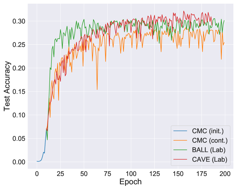
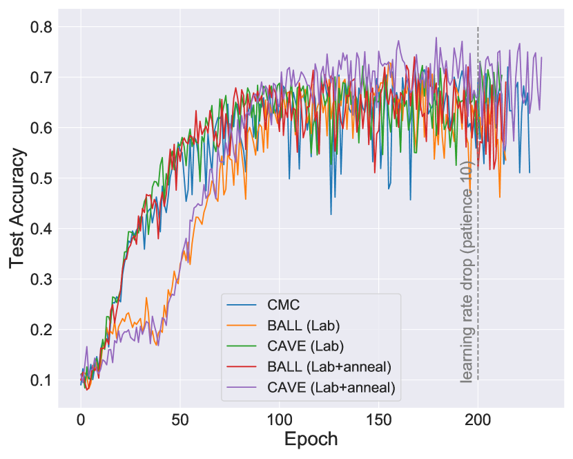
Annealing the variational distribution. Early in learning, representations may be too noisy to properly distinguish similar images when choosing negative examples (see Fig. 9). We thus consider annealing τ𝜏\tau, increasing it on each gradient step, beginning at -\infty. In the results, we use the superscript annealanneal{}^{\text{anneal}} when annealing is used. For CAVE models, annealing τ𝜏\tau will shrink the size of the set S1subscript𝑆1S_{1} defined by K-means automatically. For RING, we can choose to further anneal γ𝛾\gamma from \infty to τ𝜏\tau. That is, while we shrink the outer ball, we also enlarge the inner ball.

Model Top1 Top5 Model Top1 Top5
IR 43.2 67.0 CMC 48.2 72.4
BALL 45.3 68.6 BALLLabLab{}^{\text{Lab}} 48.9 73.1
CAVE 46.6 70.4 CAVELabLab{}^{\text{Lab}} 49.2 73.3
LA 48.0 72.4
BALLannealanneal{}_{\text{anneal}} 47.3 71.1 BALLLab+annealLab+anneal{}^{\text{Lab+anneal}} 49.7 73.6
CAVEannealanneal{}_{\text{anneal}} 48.4 72.5 CAVELab+annealLab+anneal{}^{\text{Lab+anneal}} 50.5 74.0
(a) ImageNet: Classification Accuracy
Model APbbbb{}^{\text{bb}} APbb50superscriptsubscriptabsent50bb{}_{50}^{\text{bb}} APbb75superscriptsubscriptabsent75bb{}_{75}^{\text{bb}} APmkmk{}^{\text{mk}} APmk50superscriptsubscriptabsent50mk{}_{50}^{\text{mk}} APmk75superscriptsubscriptabsent75mk{}_{75}^{\text{mk}}
IR 8.6 19.0 6.6 8.5 17.4 7.4
BALL 9.4 20.3 7.3 9.3 18.8 8.4
CAVE 9.9 21.2 7.8 9.7 19.7 8.6
LA 10.2 22.0 8.1 10.0 20.3 9.0
BALLannealanneal{}^{\text{anneal}} 9.8 21.0 7.7 9.8 19.8 8.8
CAVEannealanneal{}^{\text{anneal}} 10.7 22.8 8.5 10.7 20.9 9.4
(b) COCO: Object Detection and Inst. Segmentation
Model APkpkp{}^{\text{kp}} APkp50superscriptsubscriptabsent50kp{}_{50}^{\text{kp}} APkp75superscriptsubscriptabsent75kp{}_{75}^{\text{kp}}
IR 34.634.634.6 63.063.063.0 32.932.932.9
BALL 34.934.934.9 63.663.663.6 33.833.833.8
CAVE 35.935.935.9 64.964.964.9 34.234.234.2
LA 36.336.336.3 65.365.365.3 35.135.135.1
BALLannealanneal{}^{\text{anneal}} 36.336.336.3 65.265.265.2 35.035.035.0
CAVEannealanneal{}^{\text{anneal}} 37.037.0\mathbf{37.0} 66.166.1\mathbf{66.1} 35.635.6\mathbf{35.6}
(c) COCO: Keypoint Detection
Model APbbbb{}^{\text{bb}} APbb50superscriptsubscriptabsent50bb{}_{50}^{\text{bb}} APbb75superscriptsubscriptabsent75bb{}_{75}^{\text{bb}}
IR 5.55.55.5 14.514.514.5 3.33.33.3
BALL 6.06.06.0 15.715.715.7 3.53.53.5
CAVE 6.66.66.6 17.617.617.6 4.14.14.1
LA 7.67.6\mathbf{7.6} 20.020.020.0 4.34.3\mathbf{4.3}
BALLannealanneal{}^{\text{anneal}} 7.17.17.1 18.318.318.3 4.14.14.1
CAVEannealanneal{}^{\text{anneal}} 7.57.57.5 20.120.1\mathbf{20.1} 4.34.34.3
(d) VOC: Object Detection
Model APmkmk{}^{\text{mk}} APmk50superscriptsubscriptabsent50mk{}_{50}^{\text{mk}} APmk75superscriptsubscriptabsent75mk{}_{75}^{\text{mk}}
IR 3.03.03.0 5.95.95.9 2.82.82.8
BALL 3.43.43.4 6.56.56.5 3.33.33.3
CAVE 3.83.83.8 7.37.37.3 3.53.53.5
LA 3.83.83.8 7.27.27.2 3.53.53.5
BALLannealanneal{}^{\text{anneal}} 4.04.04.0 7.77.77.7 3.83.83.8
CAVEannealanneal{}^{\text{anneal}} 4.34.3\mathbf{4.3} 8.28.2\mathbf{8.2} 4.04.0\mathbf{4.0}
(e) LVIS: Instance Segmentation
Table 2: Evaluation of the representations using six visual transfer tasks

5 Experiments

We conduct two sets of experiments: one on CIFAR10 to compare all the objective variants, and one on ImageNet to compare select algorithms on several transfer tasks. In aggregate, we give the reader a thorough description of the algorithms uncovered by the theory and their relative performance.

Comparing negative samples and view functions. Table 1 compares 26 algorithms, of which 23 are introduced in this paper. For each algorithm, we measure its performance on classification by training a logistic regression model on the frozen representations only (see Sec. C.2).

We make a few observations: First, our simplifications to IR, CMC, and LA outperform their original implementations by up to 15%. We note that the difference between LAncence{}^{\textup{nce}} and LA is much less than the others since κ𝜅\kappa cancels from the top and bottom of the objective. Still, we see improvements due to less randomness in LAncence{}^{\textup{nce}}. Second, harder negative samples build stronger representations as BALL, RING, CAVE outperform IRncence{}^{\textup{nce}} by up to 3%. In particular, RING outperforms CAVE suggesting it as a simpler but effective alternative to K-means. Further, if we anneal in the negative distributions, we find even better performance, with gains of 3-4% over IRncence{}^{\textup{nce}}. Third, adding close neighbor views is not always beneficial: without annealing, we observe convergence to local minima as the representations cling to spurious dependencies in a noisy close neighbor set. This explains why RING even outperforms LA, which heavily relies on a well-defined neighborhood. However, with annealing, we can wait until the representation space is reasonable before adding neighbors. Together, this forms our best model, RING(Lab)+s-neigh+anneal(Lab)+s-neigh+anneal{}^{\text{(Lab)+s-neigh+anneal}}, outperforming IRncence{}^{\text{nce}} by 4%, LAncence{}^{\text{nce}} by 3%, and CMCncence{}^{\text{nce}} by 2% on CIFAR10 with gains of up to 20% without the changes to improve stability.

Comparing Transfer Tasks. Picking six algorithms, we compare their representations on five transfer tasks for a more general measure of usefulness: classification on ImageNet, object detection, instance and keypoint segmentation on COCO [11], object detection on Pascal VOC ’07 [3], and instance segmentation on LVIS [4]. Like prior work [6], we use Detectron2 [19] but with a frozen ResNet18 backbone to focus on representation quality (see Sec. C.4). From Table 2, we find more evidence of the importance of negative distributions as BALL and CAVE consistently outperform IR. Also, our best models CAVE(Lab)+annealsuperscriptCAVE(Lab)+anneal\text{CAVE}^{\text{(Lab)+anneal}} outperform IR, LA, and CMC across tasks.

6 Conclusion

We presented an interpretation of representation learning based on mutual information between image views. This formulation led to more systematic understanding of a family of existing approaches. In particular, we uncovered that the choices of views and negative sample distribution strongly influence the performance of contrastive learning. By choosing more difficult negative samples, we surpassed high-performing algorithms like LA and CMC across several visual tasks.

Several theoretical and practical questions remain. We identified the importance of views but left open questions about what makes for a “good” view. Our choice of negative examples was justified by the VINCE bound on MI. Yet VINCE is looser than InfoNCE. Future work can elucidate the relationship between learning a good representation and tightening bounds.

Broader Impact

The recent successes of machine learning may have profound societal consequences. Yet the extremely data- and compute-intensive nature of recent methods limits their availability to a small segment of society. It is urgent that we find ways to make the use of machine learning possible for a wide variety of people with a wide variety of tasks. One promising route is to solve particular tasks, with small data and little compute, by building from widely applicable and available pre-trained representations. Contrastive algorithms are becoming a popular method for unsupervised learning of representation useful for transfer tasks. This makes it important to provide a good theoretical understanding of these methods, and to make the implementations and trained representations publicly available. Our work is a step toward making these techniques clearer and better performing. We are committed to open sourcing our implementations and providing trained representations. We believe this has the potential to allow many people to solve their own tasks by building on our representations. Yet the representation learning algorithms themselves remain both data- and compute-intensive. This has the danger to provide an additional barrier to access. Future research should ameliorate this risk by committing to open access to code and trained representations, and by research ways to reduce the data or compute requirements of these methods.

References

  • [1] Ting Chen, Simon Kornblith, Mohammad Norouzi, and Geoffrey Hinton. A simple framework for contrastive learning of visual representations. arXiv preprint arXiv:2002.05709, 2020.
  • [2] Xinlei Chen, Haoqi Fan, Ross Girshick, and Kaiming He. Improved baselines with momentum contrastive learning. arXiv preprint arXiv:2003.04297, 2020.
  • [3] Mark Everingham, Luc Van Gool, Christopher KI Williams, John Winn, and Andrew Zisserman. The pascal visual object classes (voc) challenge. International journal of computer vision, 88(2):303–338, 2010.
  • [4] Agrim Gupta, Piotr Dollar, and Ross Girshick. Lvis: A dataset for large vocabulary instance segmentation. In Proceedings of the IEEE Conference on Computer Vision and Pattern Recognition, pages 5356–5364, 2019.
  • [5] Michael Gutmann and Aapo Hyvärinen. Noise-contrastive estimation: A new estimation principle for unnormalized statistical models. In Proceedings of the Thirteenth International Conference on Artificial Intelligence and Statistics, pages 297–304, 2010.
  • [6] Kaiming He, Haoqi Fan, Yuxin Wu, Saining Xie, and Ross Girshick. Momentum contrast for unsupervised visual representation learning. arXiv preprint arXiv:1911.05722, 2019.
  • [7] Kaiming He, Georgia Gkioxari, Piotr Dollár, and Ross Girshick. Mask r-cnn. In Proceedings of the IEEE international conference on computer vision, pages 2961–2969, 2017.
  • [8] Kaiming He, Xiangyu Zhang, Shaoqing Ren, and Jian Sun. Deep residual learning for image recognition. In Proceedings of the IEEE conference on computer vision and pattern recognition, pages 770–778, 2016.
  • [9] Jeff Johnson, Matthijs Douze, and Hervé Jégou. Billion-scale similarity search with gpus. IEEE Transactions on Big Data, 2019.
  • [10] Lingpeng Kong, Cyprien de Masson d’Autume, Wang Ling, Lei Yu, Zihang Dai, and Dani Yogatama. A mutual information maximization perspective of language representation learning. arXiv preprint arXiv:1910.08350, 2019.
  • [11] Tsung-Yi Lin, Michael Maire, Serge Belongie, James Hays, Pietro Perona, Deva Ramanan, Piotr Dollár, and C Lawrence Zitnick. Microsoft coco: Common objects in context. In European conference on computer vision, pages 740–755. Springer, 2014.
  • [12] Aaron van den Oord, Yazhe Li, and Oriol Vinyals. Representation learning with contrastive predictive coding. arXiv preprint arXiv:1807.03748, 2018.
  • [13] Ben Poole, Sherjil Ozair, Aaron van den Oord, Alexander A Alemi, and George Tucker. On variational bounds of mutual information. arXiv preprint arXiv:1905.06922, 2019.
  • [14] Joseph Redmon, Santosh Divvala, Ross Girshick, and Ali Farhadi. You only look once: Unified, real-time object detection. In Proceedings of the IEEE conference on computer vision and pattern recognition, pages 779–788, 2016.
  • [15] Olga Russakovsky, Jia Deng, Hao Su, Jonathan Krause, Sanjeev Satheesh, Sean Ma, Zhiheng Huang, Andrej Karpathy, Aditya Khosla, Michael Bernstein, et al. Imagenet large scale visual recognition challenge. International journal of computer vision, 115(3):211–252, 2015.
  • [16] Karen Simonyan and Andrew Zisserman. Very deep convolutional networks for large-scale image recognition. arXiv preprint arXiv:1409.1556, 2014.
  • [17] Yonglong Tian, Dilip Krishnan, and Phillip Isola. Contrastive multiview coding. arXiv preprint arXiv:1906.05849, 2019.
  • [18] Yonglong Tian, Chen Sun, Ben Poole, Dilip Krishnan, Cordelia Schmid, and Phillip Isola. What makes for good views for contrastive learning. arXiv preprint arXiv:2005.10243, 2020.
  • [19] Yuxin Wu, Alexander Kirillov, Francisco Massa, Wan-Yen Lo, and Ross Girshick. Detectron2. https://github.com/facebookresearch/detectron2, 2019.
  • [20] Zhirong Wu, Yuanjun Xiong, Stella X Yu, and Dahua Lin. Unsupervised feature learning via non-parametric instance discrimination. In Proceedings of the IEEE Conference on Computer Vision and Pattern Recognition, pages 3733–3742, 2018.
  • [21] Chengxu Zhuang, Alex Lin Zhai, and Daniel Yamins. Local aggregation for unsupervised learning of visual embeddings. In Proceedings of the IEEE International Conference on Computer Vision, pages 6002–6012, 2019.

Appendix A Proofs

A.1 Proof of Theorem 2.1

Proof.

As sums are invariant to permutation, the result is immediate. ∎

A.2 Proof of Lemma 3.1

Proof.

We focus on showing an equivalence between InfoNCE and IR, upon which its relation to CMC becomes clear. We rename X𝑋X to X1subscript𝑋1X_{1} and make K1𝐾1K-1 i.i.d. copies of X1subscript𝑋1X_{1}, named X2:Ksubscript𝑋:2𝐾X_{2:K}.

First, let the view function νIRsuperscriptsubscript𝜈IR\nu_{\textup{IR}}^{*} of index sets be defined with the standard image augmentations (cropping, flipping, color jitter, and grayscale) as used in training IR. Define an empirical estimate of (X1;νIR)subscript𝑋1superscriptsubscript𝜈IR\mathcal{I}(X_{1};\nu_{\textup{IR}}^{*}) using the dataset 𝒟𝒟\mathcal{D}. That is,

^NCE(X1;ν)=𝔼p𝒟(x1:K)𝔼A1:K,B,Bp(A)[logefθ(ν(x1,B),ν(x1,B);wB,wB)1Kj=1Kefθ(ν(x1,B}),ν(xj,Aj);wB,wAj)]{\scriptstyle\hat{\mathcal{I}}^{\text{NCE}}(X_{1};\nu^{*})=\mathbb{E}_{p_{\mathcal{D}}(x_{1:K})}\mathbb{E}_{A_{1:K},B,B^{\prime}\sim p(A)}\left[\log\frac{e^{f^{*}_{\theta}(\nu^{*}(x_{1},B),\nu^{*}(x_{1},B^{\prime});w_{B},w_{B^{\prime}})}}{\frac{1}{K}\sum_{j=1}^{K}e^{f^{*}_{\theta}(\nu^{*}(x_{1},B\}),\nu^{*}(x_{j},A_{j});w_{B},w_{A_{j}})}}\right]}

where p𝒟(x1:K)=j=1Kp𝒟(xj)subscript𝑝𝒟subscript𝑥:1𝐾superscriptsubscriptproduct𝑗1𝐾subscript𝑝𝒟subscript𝑥𝑗p_{\mathcal{D}}(x_{1:K})=\prod_{j=1}^{K}p_{\mathcal{D}}(x_{j}). In practice, we do not know p𝒟subscript𝑝𝒟p_{\mathcal{D}}, but since for all x(i)superscript𝑥𝑖x^{(i)} in 𝒟𝒟\mathcal{D}, x(i)p𝒟similar-tosuperscript𝑥𝑖subscript𝑝𝒟x^{(i)}\sim p_{\mathcal{D}}, we can sample p𝒟subscript𝑝𝒟p_{\mathcal{D}} by uniformly picking from 𝒟𝒟\mathcal{D}. So, we assume in our computation that for any xp𝒟(x)similar-to𝑥subscript𝑝𝒟𝑥x\sim p_{\mathcal{D}}(x), x𝑥x is in 𝒟𝒟\mathcal{D}. Now, define an indexing function ρ𝜌\rho that maps a sample x𝑥x from p𝒟subscript𝑝𝒟p_{\mathcal{D}} to an index in the dataset 𝒟𝒟\mathcal{D} such that xp𝒟=x(ρ(x))𝒟similar-to𝑥subscript𝑝𝒟superscript𝑥𝜌𝑥𝒟x\sim p_{\mathcal{D}}=x^{(\rho(x))}\in\mathcal{D}. This is well-formed by our assumption.

Let x1subscript𝑥1x_{1} represent the current image, a realization of X1subscript𝑋1X_{1} sampled from p𝒟(x1)subscript𝑝𝒟subscript𝑥1p_{\mathcal{D}}(x_{1}). As described in the main text, we consider a special case of ^NCE(X;ν)superscript^NCE𝑋superscript𝜈\hat{\mathcal{I}}^{\text{NCE}}(X;\nu^{*}) where the two index sets for the current image x1subscript𝑥1x_{1} are {a}𝑎\{a\}, with a𝑎a being the sampled view index in 𝒜𝒜\mathcal{A} for the current epoch of training, and A(ρ(x1))superscript𝐴𝜌subscript𝑥1A^{(\rho(x_{1}))}, the set of sampled view indices from the last nαsubscript𝑛𝛼n_{\alpha} epochs of training. Further, define weights w1={1}subscript𝑤11w_{1}=\{1\} and w2={1,α,,αnα1}subscript𝑤21𝛼superscript𝛼subscript𝑛𝛼1w_{2}=\{1,\alpha,\ldots,\alpha^{n_{\alpha}-1}\}. Then, we can rewrite the above equation as:

^NCE(X1;ν)superscript^NCEsubscript𝑋1superscript𝜈\displaystyle\scriptstyle\hat{\mathcal{I}}^{\text{NCE}}(X_{1};\nu^{*}) =𝔼p𝒟(x1:K)𝔼ap(a)[logefθ(ν(x1,{a}),ν(x1,A(ρ(x1)));w1,w2)1Kj=1Kefθ(ν(x1,{a}}),ν(xj,A(ρ(xj)));w1,w2))]\displaystyle=\scriptstyle\mathbb{E}_{p_{\mathcal{D}}(x_{1:K})}\mathbb{E}_{a\sim p(a)}\left[\log\frac{e^{f^{*}_{\theta}(\nu^{*}(x_{1},\{a\}),\nu^{*}(x_{1},A^{(\rho(x_{1}))});w_{1},w_{2})}}{\frac{1}{K}\sum_{j=1}^{K}e^{f^{*}_{\theta}(\nu^{*}(x_{1},\{a\}\}),\nu^{*}(x_{j},A^{(\rho(x_{j}))});w_{1},w_{2}))}}\right]
=𝔼p𝒟(x1:K)𝔼ap(a)[logegθ(ν(x1,a))T(k=1|Aρ(x1)|w2[k]gθ(ν(x1,A(ρ(x1))[k])))1Kj=1Kegθ(ν(x1,a))T(k=1|Aρ(x1)|w2[k]gθ(ν(x1,A(ρ(xj))[k])))]absentsubscript𝔼subscript𝑝𝒟subscript𝑥:1𝐾subscript𝔼similar-to𝑎𝑝𝑎delimited-[]superscript𝑒subscript𝑔𝜃superscript𝜈subscript𝑥1𝑎𝑇superscriptsubscript𝑘1superscript𝐴𝜌subscript𝑥1subscript𝑤2delimited-[]𝑘subscript𝑔𝜃𝜈subscript𝑥1superscript𝐴𝜌subscript𝑥1delimited-[]𝑘1𝐾superscriptsubscript𝑗1𝐾superscript𝑒subscript𝑔𝜃superscript𝜈subscript𝑥1𝑎𝑇superscriptsubscript𝑘1superscript𝐴𝜌subscript𝑥1subscript𝑤2delimited-[]𝑘subscript𝑔𝜃𝜈subscript𝑥1superscript𝐴𝜌subscript𝑥𝑗delimited-[]𝑘\displaystyle=\scriptstyle\mathbb{E}_{p_{\mathcal{D}}(x_{1:K})}\mathbb{E}_{a\sim p(a)}\left[\log\frac{e^{g_{\theta}(\nu(x_{1},a))^{T}(\sum_{k=1}^{|A^{\rho(x_{1})}|}w_{2}[k]g_{\theta}(\nu(x_{1},A^{(\rho(x_{1}))}[k])))}}{\frac{1}{K}\sum_{j=1}^{K}e^{g_{\theta}(\nu(x_{1},a))^{T}(\sum_{k=1}^{|A^{\rho(x_{1})}|}w_{2}[k]g_{\theta}(\nu(x_{1},A^{(\rho(x_{j}))}[k])))}}\right]
=𝔼p𝒟(x1:K)𝔼ap(a)[logegθ(ν(x1,a))TM[ρ(x1)]1Kj=1Kegθ(ν(x1,a))TM[ρ(xj)]]absentsubscript𝔼subscript𝑝𝒟subscript𝑥:1𝐾subscript𝔼similar-to𝑎𝑝𝑎delimited-[]superscript𝑒subscript𝑔𝜃superscript𝜈subscript𝑥1𝑎𝑇𝑀delimited-[]𝜌subscript𝑥11𝐾superscriptsubscript𝑗1𝐾superscript𝑒subscript𝑔𝜃superscript𝜈subscript𝑥1𝑎𝑇𝑀delimited-[]𝜌subscript𝑥𝑗\displaystyle=\scriptstyle\mathbb{E}_{p_{\mathcal{D}}(x_{1:K})}\mathbb{E}_{a\sim p(a)}\left[\log\frac{e^{g_{\theta}(\nu(x_{1},a))^{T}M[\rho(x_{1})]}}{\frac{1}{K}\sum_{j=1}^{K}e^{g_{\theta}(\nu(x_{1},a))^{T}M[\rho(x_{j})]}}\right]
=𝔼p𝒟(x1)[IR(x1,M)]+logKlogκabsentsubscript𝔼subscript𝑝𝒟subscript𝑥1delimited-[]superscriptIRsubscript𝑥1𝑀𝐾𝜅\displaystyle=\scriptstyle\mathbb{E}_{p_{\mathcal{D}}(x_{1})}\left[\mathcal{L}^{\textup{IR}}(x_{1},M)\right]+\log K-\log\kappa

Note that w1,w2subscript𝑤1subscript𝑤2w_{1},w_{2} are shared across the K𝐾K witness evaluations. We apply the definition of a memory bank entry in the third inequality. To see why the last equality holds, consider:

IR(x1,M)superscriptIRsubscript𝑥1𝑀\displaystyle\scriptstyle\mathcal{L}^{\textup{IR}}(x_{1},M) =𝔼p(a)[logegθ(ν(x1,a)TM[ρ(x1)]j=1Negθ(ν(x1,a)TM[ρ(xj)]]\displaystyle\scriptstyle=\mathbb{E}_{p(a)}\left[\log\frac{e^{g_{\theta}(\nu(x_{1},a)^{T}M[\rho(x_{1})]}}{\sum_{j=1}^{N}e^{g_{\theta}(\nu(x_{1},a)^{T}M[\rho(x_{j})]}}\right]
𝔼p(a)[logegθ(ν(x1,a)TM[ρ(x1)]κj=1Kegθ(ν(x1,a)TM[ρ(xj)]]\displaystyle\scriptstyle\approx\scriptstyle\mathbb{E}_{p(a)}\left[\log\frac{e^{g_{\theta}(\nu(x_{1},a)^{T}M[\rho(x_{1})]}}{\kappa\sum_{j=1}^{K}e^{g_{\theta}(\nu(x_{1},a)^{T}M[\rho(x_{j})]}}\right]
=𝔼p(a)𝔼p𝒟(x2:K)[logegθ(ν(x1,a)TM[ρ(x1)]κj=1Kegθ(ν(x1,a)TM[ρ(xj)]]\displaystyle\scriptstyle=\mathbb{E}_{p(a)}\mathbb{E}_{p_{\mathcal{D}}(x_{2:K})}\left[\log\frac{e^{g_{\theta}(\nu(x_{1},a)^{T}M[\rho(x_{1})]}}{\kappa\sum_{j=1}^{K}e^{g_{\theta}(\nu(x_{1},a)^{T}M[\rho(x_{j})]}}\right]
=𝔼p(a)𝔼p𝒟(x2:K)[logegθ(ν(x1,a)TM[ρ(x1)]1Kj=1Kegθ(ν(x1,a)TM[ρ(xj)]]logK+logκ\displaystyle\scriptstyle=\mathbb{E}_{p(a)}\mathbb{E}_{p_{\mathcal{D}}(x_{2:K})}\left[\log\frac{e^{g_{\theta}(\nu(x_{1},a)^{T}M[\rho(x_{1})]}}{\frac{1}{K}\sum_{j=1}^{K}e^{g_{\theta}(\nu(x_{1},a)^{T}M[\rho(x_{j})]}}\right]-\log K+\log\kappa

where N𝑁N is the size of the dataset 𝒟𝒟\mathcal{D}; K<N𝐾𝑁K<N is the number of samples and κ𝜅\kappa is a constant. We note that second line is an approximation already made in the original implementation of IR. Further, the third line holds since the K1𝐾1K-1 negative examples x2:Ksubscript𝑥:2𝐾x_{2:K} are sampled uniformly from the dataset 𝒟𝒟\mathcal{D}, in other words, i.i.d. from the empirical distribution, p𝒟subscript𝑝𝒟p_{\mathcal{D}}.

Having shown the equivalence between InfoNCE and IR, we move to CMC. The view set for CMC can be bisected into two: one of luminescence filters 𝒜CMC-Lsubscript𝒜CMC-L\mathcal{A}_{\textup{CMC-L}}, and one of AB-color filters 𝒜CMC-absubscript𝒜CMC-ab\mathcal{A}_{\textup{CMC-ab}}. Together, 𝒜CMC=𝒜CMC-L𝒜CMC-absubscript𝒜CMCsubscript𝒜CMC-Lsubscript𝒜CMC-ab\mathcal{A}_{\textup{CMC}}=\mathcal{A}_{\textup{CMC-L}}\cup\mathcal{A}_{\textup{CMC-ab}}. Recall that the CMC objective is a sum of two IR objectives:

CMC(x,M)=IR(xL,Mab)+IR(xab,ML)superscriptCMC𝑥𝑀superscriptIRsubscript𝑥Lsubscript𝑀absuperscriptIRsubscript𝑥absubscript𝑀L\mathcal{L}^{\textup{CMC}}(x,M)=\mathcal{L}^{\textup{IR}}(x_{\textup{L}},M_{\textup{ab}})+\mathcal{L}^{\textup{IR}}(x_{\textup{ab}},M_{\textup{L}})

So if we define two extended view functions, νCMC-L:X×2𝒜CMC-L2X:subscriptsuperscript𝜈CMC-L𝑋superscript2subscript𝒜CMC-Lsuperscript2𝑋\nu^{*}_{\text{CMC-L}}:X\times 2^{\mathcal{A}_{\textup{CMC-L}}}\rightarrow 2^{X} and νCMC-ab:X×2𝒜CMC-ab2X:subscriptsuperscript𝜈CMC-ab𝑋superscript2subscript𝒜CMC-absuperscript2𝑋\nu^{*}_{\text{CMC-ab}}:X\times 2^{\mathcal{A}_{\textup{CMC-ab}}}\rightarrow 2^{X}. Then by the above, we have ^NCE(X1;νCMC-L)𝔼p𝒟(x1)[IR(x1,L,Mab)]+logKlogκsuperscript^NCEsubscript𝑋1superscriptsubscript𝜈CMC-Lsubscript𝔼subscript𝑝𝒟subscript𝑥1delimited-[]superscriptIRsubscript𝑥1Lsubscript𝑀ab𝐾𝜅\hat{\mathcal{I}}^{\text{NCE}}(X_{1};\nu_{\text{CMC-L}}^{*})\equiv\mathbb{E}_{p_{\mathcal{D}}(x_{1})}\left[\mathcal{L}^{\textup{IR}}(x_{1,\textup{L}},M_{\textup{ab}})\right]+\log K-\log\kappa and ^NCE(X1;νCMC-ab)𝔼p𝒟(x1)[IR(x1,ab,ML)]+logKlogκsuperscript^NCEsubscript𝑋1superscriptsubscript𝜈CMC-absubscript𝔼subscript𝑝𝒟subscript𝑥1delimited-[]superscriptIRsubscript𝑥1absubscript𝑀L𝐾𝜅\hat{\mathcal{I}}^{\text{NCE}}(X_{1};\nu_{\text{CMC-ab}}^{*})\equiv\mathbb{E}_{p_{\mathcal{D}}(x_{1})}\left[\mathcal{L}^{\textup{IR}}(x_{1,\textup{ab}},M_{\textup{L}})\right]+\log K-\log\kappa. So ^NCE(X1;νCMC)𝔼p𝒟(x1)[CMC(x1,M)]/2+logKlogκsuperscript^NCEsubscript𝑋1superscriptsubscript𝜈CMCsubscript𝔼subscript𝑝𝒟subscript𝑥1delimited-[]superscriptCMCsubscript𝑥1𝑀2𝐾𝜅\hat{\mathcal{I}}^{\text{NCE}}(X_{1};\nu_{\text{CMC}}^{*})\equiv\mathbb{E}_{p_{\mathcal{D}}(x_{1})}\left[\mathcal{L}^{\textup{CMC}}(x_{1},M)\right]/2+\log K-\log\kappa where M=(ML,Mab)𝑀subscript𝑀Lsubscript𝑀abM=(M_{\textup{L}},M_{\textup{ab}}). ∎

A.3 Proof of Theorem 4.1

Proof.

It suffices to show the inequalities c<eτ𝔼T[g(x)]𝑐superscript𝑒𝜏subscript𝔼subscript𝑇delimited-[]𝑔𝑥c<e^{\tau}\leq\mathbb{E}_{\mathbb{Q}_{T}}[g(x)]. The first holds since logc<τ𝑐𝜏\log c<\tau by assumption. The second holds since 𝟏STeτ𝟏STg(x)subscript1subscript𝑆𝑇superscript𝑒𝜏subscript1subscript𝑆𝑇𝑔𝑥\mathbf{1}_{S_{T}}e^{\tau}\leq\mathbf{1}_{S_{T}}g(x), and taking the expectation 𝔼Tsubscript𝔼subscript𝑇\mathbb{E}_{\mathbb{Q}_{T}} of both sides of this inequality gives the desired result upon observing that 𝔼T[𝟏STeτ]=T(ST)eτ=eτsubscript𝔼subscript𝑇delimited-[]subscript1subscript𝑆𝑇superscript𝑒𝜏subscript𝑇subscript𝑆𝑇superscript𝑒𝜏superscript𝑒𝜏\mathbb{E}_{\mathbb{Q}_{T}}[\mathbf{1}_{S_{T}}e^{\tau}]=\mathbb{Q}_{T}(S_{T})e^{\tau}=e^{\tau} and that 𝔼T[𝟏STg(x)]=𝔼T[g(x)]subscript𝔼subscript𝑇delimited-[]subscript1subscript𝑆𝑇𝑔𝑥subscript𝔼subscript𝑇delimited-[]𝑔𝑥\mathbb{E}_{\mathbb{Q}_{T}}[\mathbf{1}_{S_{T}}g(x)]=\mathbb{E}_{\mathbb{Q}_{T}}[g(x)]. ∎

A.4 Proof of Corollary 4.1.1

Proof.

Note that each ef(x,yj)superscript𝑒𝑓𝑥subscript𝑦𝑗e^{f(x,y_{j})} for j𝑗j in [K]delimited-[]𝐾[K] satisfies the conditions on g𝑔g in Thm 4.1. So for any j𝑗j, since τ>log𝔼p(y)[ef(y1,y)]𝜏subscript𝔼𝑝𝑦delimited-[]superscript𝑒𝑓subscript𝑦1𝑦\tau>\log\mathbb{E}_{p(y)}[e^{f(y_{1},y)}], by Thm 4.1, we have that 𝔼p(yj)[ef(x,yj)]𝔼q(yj)[ef(x,yj)]subscript𝔼𝑝subscript𝑦𝑗delimited-[]superscript𝑒𝑓𝑥subscript𝑦𝑗subscript𝔼𝑞subscript𝑦𝑗delimited-[]superscript𝑒𝑓𝑥subscript𝑦𝑗\mathbb{E}_{p(y_{j})}\left[e^{f(x,y_{j})}\right]\leq\mathbb{E}_{q(y_{j})}\left[e^{f(x,y_{j})}\right]. Then by linearity of expectation, 𝔼p(x,y1)𝔼p(y2:K)[1Kj=1Kef(x,yj)]𝔼p(x,y1)𝔼q(y2:K)[1Kj=1Kef(x,yj)]subscript𝔼𝑝𝑥subscript𝑦1subscript𝔼𝑝subscript𝑦:2𝐾delimited-[]1𝐾superscriptsubscript𝑗1𝐾superscript𝑒𝑓𝑥subscript𝑦𝑗subscript𝔼𝑝𝑥subscript𝑦1subscript𝔼𝑞subscript𝑦:2𝐾delimited-[]1𝐾superscriptsubscript𝑗1𝐾superscript𝑒𝑓𝑥subscript𝑦𝑗\mathbb{E}_{p(x,y_{1})}\mathbb{E}_{p(y_{2:K})}\left[\frac{1}{K}\sum_{j=1}^{K}e^{f(x,y_{j})}\right]\leq\mathbb{E}_{p(x,y_{1})}\mathbb{E}_{q(y_{2:K})}\left[\frac{1}{K}\sum_{j=1}^{K}e^{f(x,y_{j})}\right]. Finally, let h::h:\mathbb{R}\rightarrow\mathbb{R} be any monotonic increasing function. Then, 𝔼p(x,y1)𝔼p(y2:K)[h(1Kj=1Kef(x,yj))]𝔼p(x,y1)𝔼qT(y2:K)[h(1Kj=1Kef(x,yj))]subscript𝔼𝑝𝑥subscript𝑦1subscript𝔼𝑝subscript𝑦:2𝐾delimited-[]1𝐾superscriptsubscript𝑗1𝐾superscript𝑒𝑓𝑥subscript𝑦𝑗subscript𝔼𝑝𝑥subscript𝑦1subscript𝔼subscript𝑞𝑇subscript𝑦:2𝐾delimited-[]1𝐾superscriptsubscript𝑗1𝐾superscript𝑒𝑓𝑥subscript𝑦𝑗\mathbb{E}_{p(x,y_{1})}\mathbb{E}_{p(y_{2:K})}\left[h(\frac{1}{K}\sum_{j=1}^{K}e^{f(x,y_{j})})\right]\leq\mathbb{E}_{p(x,y_{1})}\mathbb{E}_{q_{T}(y_{2:K})}\left[h(\frac{1}{K}\sum_{j=1}^{K}e^{f(x,y_{j})})\right]. But if h=logh=\log, then VINCE(X;Y1)NCE(X;Y1)superscriptVINCE𝑋subscript𝑌1superscriptNCE𝑋subscript𝑌1\mathcal{I}^{\text{VINCE}}(X;Y_{1})\leq\mathcal{I}^{\text{NCE}}(X;Y_{1}). As τ=γ𝜏𝛾-\tau\rightarrow\infty=\gamma, the bound is tight. ∎

A.5 Proof of Lemma 4.2

Proof.

We prove the more general statement for any set T𝑇T lower bounded by τ𝜏\tau, then focus on BALL as a special case. Recall that the objective we are interested in is

T(x1,M)=𝔼p(a)𝔼qT(x2:K|ν(x1,a))[logegθ(ν(x1,a))TM[ρ(x1)]/ωj=1Kegθ(ν(x1,a))TM[ρ(xj)]/ω]superscript𝑇subscript𝑥1𝑀subscript𝔼𝑝𝑎subscript𝔼subscript𝑞𝑇conditionalsubscript𝑥:2𝐾𝜈subscript𝑥1𝑎delimited-[]superscript𝑒subscript𝑔𝜃superscript𝜈subscript𝑥1𝑎𝑇𝑀delimited-[]𝜌subscript𝑥1𝜔superscriptsubscript𝑗1𝐾superscript𝑒subscript𝑔𝜃superscript𝜈subscript𝑥1𝑎𝑇𝑀delimited-[]𝜌subscript𝑥𝑗𝜔\scriptstyle\mathcal{L}^{T}(x_{1},M)=\mathbb{E}_{p(a)}\mathbb{E}_{q_{T}(x_{2:K}|\nu(x_{1},a))}\left[\log\frac{e^{g_{\theta}(\nu(x_{1},a))^{T}M[\rho(x_{1})]/\omega}}{\sum_{j=1}^{K}e^{g_{\theta}(\nu(x_{1},a))^{T}M[\rho(x_{j})]/\omega}}\right]

where x1subscript𝑥1x_{1} is a realization of random variable X1subscript𝑋1X_{1}, sampled an empirical distribution p𝒟(x1)subscript𝑝𝒟subscript𝑥1p_{\mathcal{D}}(x_{1}), and index ap(a)similar-to𝑎𝑝𝑎a\sim p(a). We call this class of objectives T𝑇T-Discrimination. By construction, T𝑇T-Discrimination uses a negative sampling distribution qTsubscript𝑞𝑇q_{T} that lies in the VINCE family of distributions. We use the notation q𝒟,Tsubscript𝑞𝒟𝑇q_{\mathcal{D},T} to refer to the empirical distribution of qTsubscript𝑞𝑇q_{T}, much like p𝒟subscript𝑝𝒟p_{\mathcal{D}} and p𝑝p. In other words, samples from q𝒟,Tsubscript𝑞𝒟𝑇q_{\mathcal{D},T} will be elements of 𝒟𝒟\mathcal{D}. Although, because q𝒟,Tsubscript𝑞𝒟𝑇q_{\mathcal{D},T} has restricted supported, not all members of 𝒟𝒟\mathcal{D}, which are sampled i.i.d. from p𝒟subscript𝑝𝒟p_{\mathcal{D}}, will be valid samples from q𝒟,Tsubscript𝑞𝒟𝑇q_{\mathcal{D},T}. By assumption, τ>log𝔼xp(x)[efθ(ν(x1,a),x)]𝜏subscript𝔼similar-to𝑥𝑝𝑥delimited-[]superscript𝑒subscript𝑓𝜃𝜈subscript𝑥1𝑎𝑥\tau>\log\mathbb{E}_{x\sim p(x)}\left[e^{f_{\theta}(\nu(x_{1},a),x)}\right], so if we can show that T𝑇T-Discrimination is equivalent to VINCE, we will get that it lower bounds mutual information between weighted view sets by Thm. 4.1.

To show the equivalence between T𝑇T-Discrimination and VINCE, we need only expand the memory bank as a weighted sum of views. Notice that gθ(ν(x1,a))=gθ(ν(x1,{a}),w1)subscript𝑔𝜃𝜈subscript𝑥1𝑎subscriptsuperscript𝑔𝜃superscript𝜈subscript𝑥1𝑎subscript𝑤1g_{\theta}(\nu(x_{1},a))=g^{*}_{\theta}(\nu^{*}(x_{1},\{a\}),w_{1}) and M[ρ(x1)]=gθ(ν(x1,A(ρ(x1))),w2)𝑀delimited-[]𝜌subscript𝑥1subscriptsuperscript𝑔𝜃superscript𝜈subscript𝑥1superscript𝐴𝜌subscript𝑥1subscript𝑤2M[\rho(x_{1})]=g^{*}_{\theta}(\nu^{*}(x_{1},A^{(\rho(x_{1}))}),w_{2}) where a𝑎a is view index at the current epoch and A(ρ(x1))superscript𝐴𝜌subscript𝑥1A^{(\rho(x_{1}))} is a set of view indices from the last nαsubscript𝑛𝛼n_{\alpha} epochs as presented in Sec. 3.1. Doing so immediately proves the statement:

𝔼p𝒟(x1)[T(x1,M)]+logKsubscript𝔼subscript𝑝𝒟subscript𝑥1delimited-[]superscript𝑇subscript𝑥1𝑀𝐾\displaystyle\scriptstyle\mathbb{E}_{p_{\mathcal{D}}(x_{1})}\left[\mathcal{L}^{T}(x_{1},M)\right]+\log K =𝔼p𝒟(x1)𝔼p(a)𝔼q𝒟,T(x2:K|ν(x1,a))[logegθ(ν(x1,a))TM[ρ(x1)]/ωj=1Kegθ(ν(x1,a))TM[ρ(xj)]/ω]+logKabsentsubscript𝔼subscript𝑝𝒟subscript𝑥1subscript𝔼𝑝𝑎subscript𝔼subscript𝑞𝒟𝑇conditionalsubscript𝑥:2𝐾𝜈subscript𝑥1𝑎delimited-[]superscript𝑒subscript𝑔𝜃superscript𝜈subscript𝑥1𝑎𝑇𝑀delimited-[]𝜌subscript𝑥1𝜔superscriptsubscript𝑗1𝐾superscript𝑒subscript𝑔𝜃superscript𝜈subscript𝑥1𝑎𝑇𝑀delimited-[]𝜌subscript𝑥𝑗𝜔𝐾\displaystyle=\scriptstyle\mathbb{E}_{p_{\mathcal{D}}(x_{1})}\mathbb{E}_{p(a)}\mathbb{E}_{q_{\mathcal{D},T}(x_{2:K}|\nu(x_{1},a))}\left[\log\frac{e^{g_{\theta}(\nu(x_{1},a))^{T}M[\rho(x_{1})]/\omega}}{\sum_{j=1}^{K}e^{g_{\theta}(\nu(x_{1},a))^{T}M[\rho(x_{j})]/\omega}}\right]+\log K
=𝔼p𝒟(x1)𝔼p(a)𝔼q𝒟,T(x2:K|ν(x1,a))[logegθ(ν(x1,{a}),w1)Tgθ(ν(x1,A(ρ(x1))),w2)/ω1Kj=1Kegθ(ν(x1,{a}),w1)Tgθ(ν(x1,A(ρ(xj))),w2)/ω]absentsubscript𝔼subscript𝑝𝒟subscript𝑥1subscript𝔼𝑝𝑎subscript𝔼subscript𝑞𝒟𝑇conditionalsubscript𝑥:2𝐾𝜈subscript𝑥1𝑎delimited-[]superscript𝑒subscriptsuperscript𝑔𝜃superscriptsuperscript𝜈subscript𝑥1𝑎subscript𝑤1𝑇subscriptsuperscript𝑔𝜃superscript𝜈subscript𝑥1superscript𝐴𝜌subscript𝑥1subscript𝑤2𝜔1𝐾superscriptsubscript𝑗1𝐾superscript𝑒subscriptsuperscript𝑔𝜃superscriptsuperscript𝜈subscript𝑥1𝑎subscript𝑤1𝑇subscriptsuperscript𝑔𝜃superscript𝜈subscript𝑥1superscript𝐴𝜌subscript𝑥𝑗subscript𝑤2𝜔\displaystyle=\scriptstyle\mathbb{E}_{p_{\mathcal{D}}(x_{1})}\mathbb{E}_{p(a)}\mathbb{E}_{q_{\mathcal{D},T}(x_{2:K}|\nu(x_{1},a))}\left[\log\frac{e^{g^{*}_{\theta}(\nu^{*}(x_{1},\{a\}),w_{1})^{T}g^{*}_{\theta}(\nu^{*}(x_{1},A^{(\rho(x_{1}))}),w_{2})/\omega}}{\frac{1}{K}\sum_{j=1}^{K}e^{g^{*}_{\theta}(\nu^{*}(x_{1},\{a\}),w_{1})^{T}g^{*}_{\theta}(\nu^{*}(x_{1},A^{(\rho(x_{j}))}),w_{2})/\omega}}\right]
=𝔼p𝒟(x1)𝔼p(a)𝔼q𝒟,T(x2:K|ν(x1,a))[logefθ(ν(x1,{a}),ν(x1,A(ρ(x1)));w1,w2)1Kj=1Kefθ(ν(x1,{a}),ν(x1,A(ρ(xj)));w1,w2)]absentsubscript𝔼subscript𝑝𝒟subscript𝑥1subscript𝔼𝑝𝑎subscript𝔼subscript𝑞𝒟𝑇conditionalsubscript𝑥:2𝐾𝜈subscript𝑥1𝑎delimited-[]superscript𝑒subscriptsuperscript𝑓𝜃superscript𝜈subscript𝑥1𝑎superscript𝜈subscript𝑥1superscript𝐴𝜌subscript𝑥1subscript𝑤1subscript𝑤21𝐾superscriptsubscript𝑗1𝐾superscript𝑒subscriptsuperscript𝑓𝜃superscript𝜈subscript𝑥1𝑎superscript𝜈subscript𝑥1superscript𝐴𝜌subscript𝑥𝑗subscript𝑤1subscript𝑤2\displaystyle=\scriptstyle\mathbb{E}_{p_{\mathcal{D}}(x_{1})}\mathbb{E}_{p(a)}\mathbb{E}_{q_{\mathcal{D},T}(x_{2:K}|\nu(x_{1},a))}\left[\log\frac{e^{f^{*}_{\theta}(\nu^{*}(x_{1},\{a\}),\nu^{*}(x_{1},A^{(\rho(x_{1}))});w_{1},w_{2})}}{\frac{1}{K}\sum_{j=1}^{K}e^{f^{*}_{\theta}(\nu^{*}(x_{1},\{a\}),\nu^{*}(x_{1},A^{(\rho(x_{j}))});w_{1},w_{2})}}\right]
=^VINCE(X1;ν)absentsuperscript^VINCEsubscript𝑋1superscript𝜈\displaystyle=\scriptstyle\hat{\mathcal{I}}^{\text{VINCE}}(X_{1};\nu^{*})

where ^VINCEsuperscript^VINCE\hat{\mathcal{I}}^{\text{VINCE}} is VINCE with respect to empirical distributions p𝒟subscript𝑝𝒟p_{\mathcal{D}}, q𝒟,Tsubscript𝑞𝒟𝑇q_{\mathcal{D},T}. In particular, since the equivalence between VINCE and T𝑇T-Discrimination holds for all T𝑇T lower bounded by τ𝜏\tau, it holds for T=[τ,)𝑇𝜏T=[\tau,\infty), which we call BALL Discrimination. ∎

A.6 Proof of Lemma 4.3

Proof.

First, we note that LA0(x(i),M)=𝔼p(a)[logp(i|x(i),M)p(B(i)|x(i),M)]superscriptLA0superscript𝑥𝑖𝑀subscript𝔼𝑝𝑎delimited-[]𝑝conditional𝑖superscript𝑥𝑖𝑀𝑝conditionalsuperscript𝐵𝑖superscript𝑥𝑖𝑀\mathcal{L}^{\text{LA${}_{0}$}}(x^{(i)},M)=\mathbb{E}_{p(a)}\left[\log\frac{p(i|x^{(i)},M)}{p(B^{(i)}|x^{(i)},M)}\right]. Say the background neighbor set B(i)superscript𝐵𝑖B^{(i)} has K𝐾K elements. By construction, we can view each element in B(i)superscript𝐵𝑖B^{(i)} as an i.i.d. sample from some VINCE distribution, q[τ,)(x|ν(x(i),a))subscript𝑞𝜏conditional𝑥𝜈superscript𝑥𝑖𝑎q_{[\tau,\infty)}(x|\nu(x^{(i)},a)) for some a𝒜𝑎𝒜a\in\mathcal{A}. This is true because we define B(i)superscript𝐵𝑖B^{(i)} programmatically by sampling uniformly from the b𝑏b closest examples (in the dataset) to the current view of the image, ν(x(i),a)𝜈superscript𝑥𝑖𝑎\nu(x^{(i)},a), where distance is measured in representation space. But because the elements from 𝒟𝒟\mathcal{D} are sampled i.i.d. from the empirical distribution p𝒟subscript𝑝𝒟p_{\mathcal{D}}, sampling uniformly from the closest b𝑏b examples is the same as sampling i.i.d. from the true marginal distribution p𝑝p but with support restricted to elements at least as close to ν(x(i),a)𝜈superscript𝑥𝑖𝑎\nu(x^{(i)},a) as the furthest element in B(i)superscript𝐵𝑖B^{(i)}. In other words, sampling from a VINCE distribution. In short, the construction of the background neighborhood is precisely equivalent to sampling from q[τ,)subscript𝑞𝜏q_{[\tau,\infty)} K𝐾K times i.i.d.

Note logp(i|x(i),M)p(B(i)|x(i),M)=log(egθ(ν(x(i)),a)TM[i]/ωjegθ(ν(x(i)),a)TM[j]/ωk=1Kegθ(ν(x(i)),a)TM[k]/ωjegθ(ν(x(i)),a)TM[j]/ω)=log(egθ(ν(x(i)),a)TM[i]/ωj=1Kegθ(ν(x(i)),a)TM[j]/ω)𝑝conditional𝑖superscript𝑥𝑖𝑀𝑝conditionalsuperscript𝐵𝑖superscript𝑥𝑖𝑀superscript𝑒subscript𝑔𝜃superscript𝜈superscript𝑥𝑖𝑎𝑇𝑀delimited-[]𝑖𝜔subscript𝑗superscript𝑒subscript𝑔𝜃superscript𝜈superscript𝑥𝑖𝑎𝑇𝑀delimited-[]𝑗𝜔superscriptsubscript𝑘1𝐾superscript𝑒subscript𝑔𝜃superscript𝜈superscript𝑥𝑖𝑎𝑇𝑀delimited-[]𝑘𝜔subscript𝑗superscript𝑒subscript𝑔𝜃superscript𝜈superscript𝑥𝑖𝑎𝑇𝑀delimited-[]𝑗𝜔superscript𝑒subscript𝑔𝜃superscript𝜈superscript𝑥𝑖𝑎𝑇𝑀delimited-[]𝑖𝜔superscriptsubscript𝑗1𝐾superscript𝑒subscript𝑔𝜃superscript𝜈superscript𝑥𝑖𝑎𝑇𝑀delimited-[]𝑗𝜔\log\frac{p(i|x^{(i)},M)}{p(B^{(i)}|x^{(i)},M)}=\log\left(\frac{\frac{e^{g_{\theta}(\nu(x^{(i)}),a)^{T}M[i]/\omega}}{\sum_{j}e^{g_{\theta}(\nu(x^{(i)}),a)^{T}M[j]/\omega}}}{\frac{\sum_{k=1}^{K}e^{g_{\theta}(\nu(x^{(i)}),a)^{T}M[k]/\omega}}{\sum_{j}e^{g_{\theta}(\nu(x^{(i)}),a)^{T}M[j]/\omega}}}\right)=\log\left(\frac{e^{g_{\theta}(\nu(x^{(i)}),a)^{T}M[i]/\omega}}{\sum_{j=1}^{K}e^{g_{\theta}(\nu(x^{(i)}),a)^{T}M[j]/\omega}}\right) . So LA0(x1,M)=𝔼p(a)𝔼q[τ,)(x2:K|ν(x1,a))[log(egθ(ν(x1),a)TM[ρ(xi)]/ωj=1Kegθ(ν(x1),a)TM[ρ(xj)]/ω)]=BALL(x1,M)superscriptLA0subscript𝑥1𝑀subscript𝔼𝑝𝑎subscript𝔼subscript𝑞𝜏conditionalsubscript𝑥:2𝐾𝜈subscript𝑥1𝑎delimited-[]superscript𝑒subscript𝑔𝜃superscript𝜈subscript𝑥1𝑎𝑇𝑀delimited-[]𝜌subscript𝑥𝑖𝜔superscriptsubscript𝑗1𝐾superscript𝑒subscript𝑔𝜃superscript𝜈subscript𝑥1𝑎𝑇𝑀delimited-[]𝜌subscript𝑥𝑗𝜔superscriptBALLsubscript𝑥1𝑀\mathcal{L}^{\text{LA${}_{0}$}}(x_{1},M)=\mathbb{E}_{p(a)}\mathbb{E}_{q_{[\tau,\infty)}(x_{2:K}|\nu(x_{1},a))}\left[\log\left(\frac{e^{g_{\theta}(\nu(x_{1}),a)^{T}M[\rho(x_{i})]/\omega}}{\sum_{j=1}^{K}e^{g_{\theta}(\nu(x_{1}),a)^{T}M[\rho(x_{j})]/\omega}}\right)\right]=\mathcal{L}^{\text{BALL}}(x_{1},M) where ρ𝜌\rho is a function realizations of X𝑋X to an index in [1,|𝒟|]1𝒟[1,|\mathcal{D}|] as defined in Sec. A.2. ∎

A.7 Proof of Lemma 4.4

Proof.

Take the i𝑖i-th from the dataset 𝒟𝒟\mathcal{D}, x(i)superscript𝑥𝑖x^{(i)}. Then let C(i)superscript𝐶𝑖C^{(i)} be the close neighbor set for x(i)superscript𝑥𝑖x^{(i)} and B(i)superscript𝐵𝑖B^{(i)} the background neighbor set for x(i)superscript𝑥𝑖x^{(i)} as defined in LA. Let N𝑁N be the number of elements in C(i)B(i)=C(i)superscript𝐶𝑖superscript𝐵𝑖superscript𝐶𝑖C^{(i)}\cap B^{(i)}=C^{(i)}. Now, we can show the following

LA(x(i),M)logNsuperscriptLAsuperscript𝑥𝑖𝑀𝑁\displaystyle\scriptstyle\mathcal{L}^{\text{LA}}(x^{(i)},M)-\log N =log(p(C(i)B(i)|x(i),M)p(B(i)|x(i),M))logNabsent𝑝superscript𝐶𝑖conditionalsuperscript𝐵𝑖superscript𝑥𝑖𝑀𝑝conditionalsuperscript𝐵𝑖superscript𝑥𝑖𝑀𝑁\displaystyle=\scriptstyle\log\left(\frac{p(C^{(i)}\cap B^{(i)}|x^{(i)},M)}{p(B^{(i)}|x^{(i)},M)}\right)-\log N
=log(𝔼p(a)[1NkC(i)B(i)e(gθ(ν(x(i),a))TM[k]/ω)/Z]p(B(i)|x(i),M))absentsubscript𝔼𝑝𝑎delimited-[]1𝑁subscript𝑘superscript𝐶𝑖superscript𝐵𝑖superscript𝑒subscript𝑔𝜃superscript𝜈superscript𝑥𝑖𝑎𝑇𝑀delimited-[]𝑘𝜔𝑍𝑝conditionalsuperscript𝐵𝑖superscript𝑥𝑖𝑀\displaystyle\scriptstyle=\log\left(\frac{\mathbb{E}_{p(a)}\left[\frac{1}{N}\sum_{k\in C^{(i)}\cap B^{(i)}}e^{(g_{\theta}(\nu(x^{(i)},a))^{T}M[k]/\omega)}/Z\right]}{p(B^{(i)}|x^{(i)},M)}\right)
log(𝔼p(a)[e(gθ(ν(x(i),a))TM[i]/ω)/Z]p(B(i)|x(i),M))absentsubscript𝔼𝑝𝑎delimited-[]superscript𝑒subscript𝑔𝜃superscript𝜈superscript𝑥𝑖𝑎𝑇𝑀delimited-[]𝑖𝜔𝑍𝑝conditionalsuperscript𝐵𝑖superscript𝑥𝑖𝑀\displaystyle\scriptstyle\leq\log\left(\frac{\mathbb{E}_{p(a)}\left[e^{(g_{\theta}(\nu(x^{(i)},a))^{T}M[i]/\omega)}/Z\right]}{p(B^{(i)}|x^{(i)},M)}\right)
=log(p(i|xi,M)p(Bi|xi,M))=LA0(x(i),M)absent𝑝conditional𝑖subscript𝑥𝑖𝑀𝑝conditionalsubscript𝐵𝑖subscript𝑥𝑖𝑀superscriptsubscriptLA0superscript𝑥𝑖𝑀\displaystyle\scriptstyle=\log\left(\frac{p(i|x_{i},M)}{p(B_{i}|x_{i},M)}\right)=\mathcal{L}^{\text{LA}_{0}}(x^{(i)},M)

where we use Z𝑍Z to abbreviate the denominator of p(i|x(i),M)𝑝conditional𝑖superscript𝑥𝑖𝑀p(i|x^{(i)},M). The inequality in the third line holds since adding noise to a vector decreases its correlation with any other vector. In other words, of all entries in the memory bank, M[i]𝑀delimited-[]𝑖M[i] is at least as close to gθ(ν(x(i),a))subscript𝑔𝜃𝜈superscript𝑥𝑖𝑎g_{\theta}(\nu(x^{(i)},a)) as any other entry M[j]𝑀delimited-[]𝑗M[j] for any a𝒜𝑎𝒜a\in\mathcal{A}. Hence, gθ(ν(x(i),a))TM[i]gθ(ν(x(i),a))TM[j]subscript𝑔𝜃superscript𝜈superscript𝑥𝑖𝑎𝑇𝑀delimited-[]𝑖subscript𝑔𝜃superscript𝜈superscript𝑥𝑖𝑎𝑇𝑀delimited-[]𝑗g_{\theta}(\nu(x^{(i)},a))^{T}M[i]\geq g_{\theta}(\nu(x^{(i)},a))^{T}M[j] for any ji𝑗𝑖j\neq i. ∎

A.8 Proof of InfoNCE

Lemmas A.1A.2 and Thm. A.3 are largely taken from [13]. We will start with a simpler estimator of mutual information, known as the Barber-Agakov estimator, and work our way to InfoNCE.

Lemma A.1.

Define the (normalized) Barber-Agakov bound as BA(X;Y)=𝔼p(x,y)[logq(x|y)logp(x)]superscriptBA𝑋𝑌subscript𝔼𝑝𝑥𝑦delimited-[]𝑞conditional𝑥𝑦𝑝𝑥\mathcal{I}^{\textup{BA}}(X;Y)=\mathbb{E}_{p(x,y)}\left[\log q(x|y)-\log p(x)\right] where q(x|y)𝑞conditional𝑥𝑦q(x|y) is a variational distribution approximating p(x|y)𝑝conditional𝑥𝑦p(x|y). Then (X;Y)BA(X;Y)𝑋𝑌superscriptBA𝑋𝑌\mathcal{I}(X;Y)\geq\mathcal{I}^{\textup{BA}}(X;Y). If we let q(x|y)=p(x)ef(x,y)Z(y)𝑞conditional𝑥𝑦𝑝𝑥superscript𝑒𝑓𝑥𝑦𝑍𝑦q(x|y)=\frac{p(x)e^{f(x,y)}}{Z(y)} where f(x,y)𝑓𝑥𝑦f(x,y) is the witness function and Z(y)=𝔼p(x)[ef(x,y)]𝑍𝑦subscript𝔼𝑝𝑥delimited-[]superscript𝑒𝑓𝑥𝑦Z(y)=\mathbb{E}_{p(x)}[e^{f(x,y)}] is the partition, define the unnormalized Barber-Agakov bound as UBA(X;Y)=𝔼p(x,y)[f(x,y)logZ(y)]superscriptUBA𝑋𝑌subscript𝔼𝑝𝑥𝑦delimited-[]𝑓𝑥𝑦𝑍𝑦\mathcal{I}^{\textup{UBA}}(X;Y)=\mathbb{E}_{p(x,y)}\left[f(x,y)-\log Z(y)\right] Then, (X;Y)UBA(X;Y)𝑋𝑌superscriptUBA𝑋𝑌\mathcal{I}(X;Y)\geq\mathcal{I}^{\textup{UBA}}(X;Y).

Proof.

We first observe that (X;Y)=𝔼p(x,y)[logp(x|y)p(x)]=𝔼p(x,y)[logq(x|y)p(x|y)p(x)q(x|y)]=𝔼p(x,y)[logq(x|y)p(x)]+𝒟KL(p(x|y)||q(x|y))𝔼p(x,y)[logq(x|y)p(x)]=BA(X;Y)\mathcal{I}(X;Y)=\mathbb{E}_{p(x,y)}\left[\log\frac{p(x|y)}{p(x)}\right]=\mathbb{E}_{p(x,y)}\left[\log\frac{q(x|y)p(x|y)}{p(x)q(x|y)}\right]=\mathbb{E}_{p(x,y)}\left[\log\frac{q(x|y)}{p(x)}\right]+\mathcal{D}_{\text{KL}}(p(x|y)||q(x|y))\geq\mathbb{E}_{p(x,y)}\left[\log\frac{q(x|y)}{p(x)}\right]=\mathcal{I}^{\textup{BA}}(X;Y). For the unnormalized bound, use the definition for q(x|y)𝑞conditional𝑥𝑦q(x|y). Lastly, (X;Y)𝔼p(x,y)[logq(x|y)p(x)]=𝔼p(x,y)[logp(x)ef(x,y)p(x)Z(y)]=𝔼p(x,y)[f(x,y)logZ(y)]=UBA(X;Y)𝑋𝑌subscript𝔼𝑝𝑥𝑦delimited-[]𝑞conditional𝑥𝑦𝑝𝑥subscript𝔼𝑝𝑥𝑦delimited-[]𝑝𝑥superscript𝑒𝑓𝑥𝑦𝑝𝑥𝑍𝑦subscript𝔼𝑝𝑥𝑦delimited-[]𝑓𝑥𝑦𝑍𝑦superscriptUBA𝑋𝑌\mathcal{I}(X;Y)\geq\mathbb{E}_{p(x,y)}\left[\log\frac{q(x|y)}{p(x)}\right]=\mathbb{E}_{p(x,y)}\left[\log\frac{p(x)e^{f(x,y)}}{p(x)Z(y)}\right]=\mathbb{E}_{p(x,y)}\left[f(x,y)-\log Z(y)\right]=\mathcal{I}^{\textup{UBA}}(X;Y). ∎

The log-partition logZ(y)𝑍𝑦\log Z(y) is difficult to evaluate. The next estimator bounds it instead.

Lemma A.2.

Define the Nguyen-Wainwright-Jordan bound as NWJ(X;Y)=𝔼p(x,y)[f(x,y)]𝔼p(y)[1eZ(y)]superscriptNWJ𝑋𝑌subscript𝔼𝑝𝑥𝑦delimited-[]𝑓𝑥𝑦subscript𝔼𝑝𝑦delimited-[]1𝑒𝑍𝑦\mathcal{I}^{\textup{NWJ}}(X;Y)=\mathbb{E}_{p(x,y)}\left[f(x,y)\right]-\mathbb{E}_{p(y)}\left[\frac{1}{e}Z(y)\right] where Z(y)𝑍𝑦Z(y) is defined as in Lemma A.1. Then (X;Y)NWJ(X;Y)𝑋𝑌superscriptNWJ𝑋𝑌\mathcal{I}(X;Y)\geq\mathcal{I}^{\textup{NWJ}}(X;Y).

Proof.

For a(y)𝑎𝑦a(y) positive we use the bound logZ(y)Z(y)a(y)+loga(y)1𝑍𝑦𝑍𝑦𝑎𝑦𝑎𝑦1\log Z(y)\leq\frac{Z(y)}{a(y)}+\log a(y)-1, tight when a(y)=Z(y)𝑎𝑦𝑍𝑦a(y)=Z(y). Use this on UBA(X;Y)superscriptUBA𝑋𝑌\mathcal{I}^{\textup{UBA}}(X;Y). (X;Y)UBA(X;Y)=𝔼p(x,y)[f(x,y)]𝔼p(y)[logZ(y)]𝔼p(x,y)[f(x,y)]𝔼p(y)[Z(y)a(y)+loga(y)1]=𝔼p(x,y)[f(x,y)]𝔼p(y)[1a(y)𝔼p(x)[ef(x,y)]+loga(y)1]𝑋𝑌superscriptUBA𝑋𝑌subscript𝔼𝑝𝑥𝑦delimited-[]𝑓𝑥𝑦subscript𝔼𝑝𝑦delimited-[]𝑍𝑦subscript𝔼𝑝𝑥𝑦delimited-[]𝑓𝑥𝑦subscript𝔼𝑝𝑦delimited-[]𝑍𝑦𝑎𝑦𝑎𝑦1subscript𝔼𝑝𝑥𝑦delimited-[]𝑓𝑥𝑦subscript𝔼𝑝𝑦delimited-[]1𝑎𝑦subscript𝔼𝑝𝑥delimited-[]superscript𝑒𝑓𝑥𝑦𝑎𝑦1\mathcal{I}(X;Y)\geq\mathcal{I}^{\textup{UBA}}(X;Y)=\mathbb{E}_{p(x,y)}\left[f(x,y)\right]-\mathbb{E}_{p(y)}\left[\log Z(y)\right]\geq\mathbb{E}_{p(x,y)}\left[f(x,y)\right]-\mathbb{E}_{p(y)}\left[\frac{Z(y)}{a(y)}+\log a(y)-1\right]=\mathbb{E}_{p(x,y)}\left[f(x,y)\right]-\mathbb{E}_{p(y)}\left[\frac{1}{a(y)}\mathbb{E}_{p(x)}[e^{f(x,y)}]+\log a(y)-1\right]. Now, choose a(y)=e𝑎𝑦𝑒a(y)=e. Then, (X;Y)𝔼p(x,y)[f(x,y)]𝔼p(y)[1e𝔼p(x)[ef(x,y)]+loge1]=𝔼p(x,y)[f(x,y)]𝔼p(y)[Z(y)e]=NWJ(X;Y)𝑋𝑌subscript𝔼𝑝𝑥𝑦delimited-[]𝑓𝑥𝑦subscript𝔼𝑝𝑦delimited-[]1𝑒subscript𝔼𝑝𝑥delimited-[]superscript𝑒𝑓𝑥𝑦𝑒1subscript𝔼𝑝𝑥𝑦delimited-[]𝑓𝑥𝑦subscript𝔼𝑝𝑦delimited-[]𝑍𝑦𝑒superscriptNWJ𝑋𝑌\mathcal{I}(X;Y)\geq\mathbb{E}_{p(x,y)}\left[f(x,y)\right]-\mathbb{E}_{p(y)}\left[\frac{1}{e}\mathbb{E}_{p(x)}[e^{f(x,y)}]+\log e-1\right]=\mathbb{E}_{p(x,y)}\left[f(x,y)\right]-\mathbb{E}_{p(y)}\left[\frac{Z(y)}{e}\right]=\mathcal{I}^{\textup{NWJ}}(X;Y)

Finally, we are ready to show that the InfoNCE estimator lower bounds mutual information. One of primary differences between the NWJ and the InfoNCE estimators is that the latter reuses the sample y𝑦y from the joint p(x,y)𝑝𝑥𝑦p(x,y) in estimating the partition.

Theorem A.3.

Let X𝑋X, Y1,,YKsubscript𝑌1subscript𝑌𝐾Y_{1},...,Y_{K} be two random variables with the Yjsubscript𝑌𝑗Y_{j} i.i.d. for j=1,,K𝑗1𝐾j=1,...,K. Let K1𝐾1K-1 be the number of negative samples. Define p(x,y1)𝑝𝑥subscript𝑦1p(x,y_{1}) as the joint distribution for X𝑋X and Y1subscript𝑌1Y_{1}. Define p(y2:K)=j=2Kp(yj)𝑝subscript𝑦:2𝐾superscriptsubscriptproduct𝑗2𝐾𝑝subscript𝑦𝑗p(y_{2:K})=\prod_{j=2}^{K}p(y_{j}) as the distribution over negative samples. Fix p(yj)=p(y1)𝑝subscript𝑦𝑗𝑝subscript𝑦1p(y_{j})=p(y_{1}), the marginal distribution for Y1subscript𝑌1Y_{1}. Recall the InfoNCE estimator

NCE(X;Y1)=𝔼p(x,y1)[fθ,ϕ(x,y1)𝔼p(y2:K)[log1Kj=1Kefθ,ϕ(x,yj)]]superscriptNCE𝑋subscript𝑌1subscript𝔼𝑝𝑥subscript𝑦1delimited-[]subscript𝑓𝜃italic-ϕ𝑥subscript𝑦1subscript𝔼𝑝subscript𝑦:2𝐾delimited-[]1𝐾superscriptsubscript𝑗1𝐾superscript𝑒subscript𝑓𝜃italic-ϕ𝑥subscript𝑦𝑗\scriptstyle\mathcal{I}^{\textup{NCE}}(X;Y_{1})=\mathbb{E}_{p(x,y_{1})}\left[f_{\theta,\phi}(x,y_{1})-\mathbb{E}_{p(y_{2:K})}\left[\log\frac{1}{K}\sum_{j=1}^{K}e^{f_{\theta,\phi}(x,y_{j})}\right]\right]

. Then, (X;Y1)NCE(X,Y1)𝑋subscript𝑌1superscriptNCE𝑋subscript𝑌1\mathcal{I}(X;Y_{1})\geq\mathcal{I}^{\textup{NCE}}(X,Y_{1}). That is, the InfoNCE objective is a lower bound for the mutual information between X𝑋X and Y1subscript𝑌1Y_{1}.

Proof.

We will show that the InfoNCE bound arises from augmenting y1subscript𝑦1y_{1} with a set of auxiliary samples y2,,yKsubscript𝑦2subscript𝑦𝐾y_{2},...,y_{K} and employ the Nguyen-Wainwright-Jordan bound.

Let Y2:Ksubscript𝑌:2𝐾Y_{2:K} be a set of random variables distributed independently according to p(y1)𝑝subscript𝑦1p(y_{1}). As Y1subscript𝑌1Y_{1} and Y2:Ksubscript𝑌:2𝐾Y_{2:K} are independent, (X;Y1)=(X;Y1,Y2:K)𝑋subscript𝑌1𝑋subscript𝑌1subscript𝑌:2𝐾\mathcal{I}(X;Y_{1})=\mathcal{I}(X;Y_{1},Y_{2:K}). Now assume a witness function: f(x,y1:K)=1+logef(x,y1)a(x,y1:K)𝑓𝑥subscript𝑦:1𝐾1superscript𝑒𝑓𝑥subscript𝑦1𝑎𝑥subscript𝑦:1𝐾f(x,y_{1:K})=1+\log\frac{e^{f(x,y_{1})}}{a(x,y_{1:K})}, where a(x,y1:K)=1Ki=1Kef(x,yi)𝑎𝑥subscript𝑦:1𝐾1𝐾superscriptsubscript𝑖1𝐾superscript𝑒𝑓𝑥subscript𝑦𝑖a(x,y_{1:K})=\frac{1}{K}\sum_{i=1}^{K}e^{f(x,y_{i})}, a Monte Carlo approximation of the partition Z(y)𝑍𝑦Z(y). Apply the Nguyen-Wainwright-Jordan bound. (X;Y1)=(X;Y1,Y2:K)𝔼p(x,y1:K)[1+logef(x,y1)a(x,y1:K)]𝔼p(x)p(y1:K)[1ee1+logef(x,y1)a(x,y1:K)]=1+𝔼p(x,y1:K)[logef(x,y1)a(x,y1:K)]𝔼p(x)p(y1:K)[ef(x,y1)a(x,y1:K)]𝑋subscript𝑌1𝑋subscript𝑌1subscript𝑌:2𝐾subscript𝔼𝑝𝑥subscript𝑦:1𝐾delimited-[]1superscript𝑒𝑓𝑥subscript𝑦1𝑎𝑥subscript𝑦:1𝐾subscript𝔼𝑝𝑥𝑝subscript𝑦:1𝐾delimited-[]1𝑒superscript𝑒1superscript𝑒𝑓𝑥subscript𝑦1𝑎𝑥subscript𝑦:1𝐾1subscript𝔼𝑝𝑥subscript𝑦:1𝐾delimited-[]superscript𝑒𝑓𝑥subscript𝑦1𝑎𝑥subscript𝑦:1𝐾subscript𝔼𝑝𝑥𝑝subscript𝑦:1𝐾delimited-[]superscript𝑒𝑓𝑥subscript𝑦1𝑎𝑥subscript𝑦:1𝐾\mathcal{I}(X;Y_{1})=\mathcal{I}(X;Y_{1},Y_{2:K})\geq\mathbb{E}_{p(x,y_{1:K})}\left[1+\log\frac{e^{f(x,y_{1})}}{a(x,y_{1:K})}\right]-\mathbb{E}_{p(x)p(y_{1:K})}\left[\frac{1}{e}\cdot e^{1+\log\frac{e^{f(x,y_{1})}}{a(x,y_{1:K})}}\right]=1+\mathbb{E}_{p(x,y_{1:K})}\left[\log\frac{e^{f(x,y_{1})}}{a(x,y_{1:K})}\right]-\mathbb{E}_{p(x)p(y_{1:K})}\left[\frac{e^{f(x,y_{1})}}{a(x,y_{1:K})}\right] Because p(y1:K)=ip(yi)𝑝subscript𝑦:1𝐾subscriptproduct𝑖𝑝subscript𝑦𝑖p(y_{1:K})=\prod_{i}p(y_{i}) is invariant under permutation of indices 1:K:1𝐾{1:K}, we have 𝔼p(x)p(y1:K)[ef(x,y1)a(x,y1:K)]=𝔼p(x)p(y1:K)[ef(x,yi)a(x,y1:K)]subscript𝔼𝑝𝑥𝑝subscript𝑦:1𝐾delimited-[]superscript𝑒𝑓𝑥subscript𝑦1𝑎𝑥subscript𝑦:1𝐾subscript𝔼𝑝𝑥𝑝subscript𝑦:1𝐾delimited-[]superscript𝑒𝑓𝑥subscript𝑦𝑖𝑎𝑥subscript𝑦:1𝐾\mathbb{E}_{p(x)p(y_{1:K})}\left[\frac{e^{f(x,y_{1})}}{a(x,y_{1:K})}\right]=\mathbb{E}_{p(x)p(y_{1:K})}\left[\frac{e^{f(x,y_{i})}}{a(x,y_{1:K})}\right] for any i𝑖i. Use this and the definition of a𝑎a: 𝔼p(x)p(y1:K)[ef(x,y1)a(x,y1:K)]=1Ki=1K𝔼p(x)p(y1:K)[ef(x,yi)a(x,y1:K)]=𝔼p(x)p(y1:K)[1Ki=1Kef(x,yi)a(x,y1:K)]=1subscript𝔼𝑝𝑥𝑝subscript𝑦:1𝐾delimited-[]superscript𝑒𝑓𝑥subscript𝑦1𝑎𝑥subscript𝑦:1𝐾1𝐾superscriptsubscript𝑖1𝐾subscript𝔼𝑝𝑥𝑝subscript𝑦:1𝐾delimited-[]superscript𝑒𝑓𝑥subscript𝑦𝑖𝑎𝑥subscript𝑦:1𝐾subscript𝔼𝑝𝑥𝑝subscript𝑦:1𝐾delimited-[]1𝐾superscriptsubscript𝑖1𝐾superscript𝑒𝑓𝑥subscript𝑦𝑖𝑎𝑥subscript𝑦:1𝐾1\mathbb{E}_{p(x)p(y_{1:K})}\left[\frac{e^{f(x,y_{1})}}{a(x,y_{1:K})}\right]=\frac{1}{K}\sum_{i=1}^{K}\mathbb{E}_{p(x)p(y_{1:K})}\left[\frac{e^{f(x,y_{i})}}{a(x,y_{1:K})}\right]=\mathbb{E}_{p(x)p(y_{1:K})}\left[\frac{\frac{1}{K}\sum_{i=1}^{K}e^{f(x,y_{i})}}{a(x,y_{1:K})}\right]=1 We now substitute this result into full equation above: (X;Y1)1+𝔼p(x,y1:K)[logef(x,y1)a(x,y1:K)]1=𝔼p(x,y1:K)[f(x,y1)log1Ki=1Kef(x,yi)]=𝔼p(x,y1)𝔼p(y2:K)[f(x,y1)log1Ki=1Kef(x,yi)]=NCE(X;Y1)𝑋subscript𝑌11subscript𝔼𝑝𝑥subscript𝑦:1𝐾delimited-[]superscript𝑒𝑓𝑥subscript𝑦1𝑎𝑥subscript𝑦:1𝐾1subscript𝔼𝑝𝑥subscript𝑦:1𝐾delimited-[]𝑓𝑥subscript𝑦11𝐾superscriptsubscript𝑖1𝐾superscript𝑒𝑓𝑥subscript𝑦𝑖subscript𝔼𝑝𝑥subscript𝑦1subscript𝔼𝑝subscript𝑦:2𝐾delimited-[]𝑓𝑥subscript𝑦11𝐾superscriptsubscript𝑖1𝐾superscript𝑒𝑓𝑥subscript𝑦𝑖superscriptNCE𝑋subscript𝑌1\mathcal{I}(X;Y_{1})\geq 1+\mathbb{E}_{p(x,y_{1:K})}\left[\log\frac{e^{f(x,y_{1})}}{a(x,y_{1:K})}\right]-1=\mathbb{E}_{p(x,y_{1:K})}\left[f(x,y_{1})-\log\frac{1}{K}\sum_{i=1}^{K}e^{f(x,y_{i})}\right]=\mathbb{E}_{p(x,y_{1})}\mathbb{E}_{p(y_{2:K})}\left[f(x,y_{1})-\log\frac{1}{K}\sum_{i=1}^{K}e^{f(x,y_{i})}\right]=\mathcal{I}^{\textup{NCE}}(X;Y_{1})

Appendix B Additional lemmas

In the main text, we owe the reader a few additional lemmas.

Lemma B.1.

Define the SimCLR objective (with explicit data augmentation) as SimCLR(x1)=𝔼a1:K,b,bp(a)[ehψ(uϕ(ν(x1,b)))Thψ(uϕ(ν(x1,b)))/ωj=1Kehψ(uϕ(ν(x1,b)))Thψ(uϕ(ν(xj,aj)))/ω]superscriptSimCLRsubscript𝑥1subscript𝔼similar-tosubscript𝑎:1𝐾𝑏superscript𝑏𝑝𝑎delimited-[]superscript𝑒subscript𝜓superscriptsubscript𝑢italic-ϕ𝜈subscript𝑥1𝑏𝑇subscript𝜓subscript𝑢italic-ϕ𝜈subscript𝑥1superscript𝑏𝜔superscriptsubscript𝑗1𝐾superscript𝑒subscript𝜓superscriptsubscript𝑢italic-ϕ𝜈subscript𝑥1𝑏𝑇subscript𝜓subscript𝑢italic-ϕ𝜈subscript𝑥𝑗subscript𝑎𝑗𝜔\mathcal{L}^{\textup{SimCLR}}(x_{1})=\mathbb{E}_{a_{1:K},b,b^{\prime}\sim p(a)}\left[\frac{e^{h_{\psi}(u_{\phi}(\nu(x_{1},b)))^{T}h_{\psi}(u_{\phi}(\nu(x_{1},b^{\prime})))/\omega}}{\sum_{j=1}^{K}e^{h_{\psi}(u_{\phi}(\nu(x_{1},b)))^{T}h_{\psi}(u_{\phi}(\nu(x_{j},a_{j})))/\omega}}\right] where hψsubscript𝜓h_{\psi} and uϕsubscript𝑢italic-ϕu_{\phi} are two encoders, usually neural networks, and ν𝜈\nu is a view function. Assume we have a dataset 𝒟𝒟\mathcal{D} sampled i.i.d. from an empirical distribution p𝒟subscript𝑝𝒟p_{\mathcal{D}}. Let K𝐾K be the size of minibatch. Then, 𝔼p𝒟(x1)[SimCLR(x1)]+logK=^NCE(X;ν)subscript𝔼subscript𝑝𝒟subscript𝑥1delimited-[]superscriptSimCLRsubscript𝑥1𝐾superscript^NCE𝑋𝜈\mathbb{E}_{p_{\mathcal{D}}(x_{1})}\left[\mathcal{L}^{\text{SimCLR}}(x_{1})\right]+\log K=\hat{\mathcal{I}}^{\text{NCE}}(X;\nu), an empirical estimate of InfoNCE between two views of X𝑋X.

Proof.

Let the empirical estimate of InfoNCE between two views be ^NCE(X;ν)=𝔼p𝒟(x1:K)𝔼a1:N,b,bp(a)[logefθ(ν(x1,b),ν(x1,b))1Kj=1Kefθ(ν(x1,b),ν(xj,aj))]superscript^NCE𝑋𝜈subscript𝔼subscript𝑝𝒟subscript𝑥:1𝐾subscript𝔼similar-tosubscript𝑎:1𝑁𝑏superscript𝑏𝑝𝑎delimited-[]superscript𝑒subscript𝑓𝜃𝜈subscript𝑥1𝑏𝜈subscript𝑥1superscript𝑏1𝐾superscriptsubscript𝑗1𝐾superscript𝑒subscript𝑓𝜃𝜈subscript𝑥1𝑏𝜈subscript𝑥𝑗subscript𝑎𝑗\hat{\mathcal{I}}^{\text{NCE}}(X;\nu)=\mathbb{E}_{p_{\mathcal{D}}(x_{1:K})}\mathbb{E}_{a_{1:N},b,b^{\prime}\sim p(a)}\left[\log\frac{e^{f_{\theta}(\nu(x_{1},b),\nu(x_{1},b^{\prime}))}}{\frac{1}{K}\sum_{j=1}^{K}e^{f_{\theta}(\nu(x_{1},b),\nu(x_{j},a_{j}))}}\right]. Now, define gθ=hψuϕsubscript𝑔𝜃subscript𝜓subscript𝑢italic-ϕg_{\theta}=h_{\psi}\circ u_{\phi} where θ=ψϕ𝜃𝜓italic-ϕ\theta=\psi\cup\phi, the composition of the two functions. Now, we see

SimCLR(x1)+logKsuperscriptSimCLRsubscript𝑥1𝐾\displaystyle\mathcal{L}^{\textup{SimCLR}}(x_{1})+\log K =𝔼a1:K,b,bp(a)[ehψ(uϕ(ν(x1,b)))Thψ(uϕ(ν(x1,b)))/ωj=1Kehψ(uϕ(ν(x1,b)))Thψ(uϕ(ν(xj,aj)))/ω]+logKabsentsubscript𝔼similar-tosubscript𝑎:1𝐾𝑏superscript𝑏𝑝𝑎delimited-[]superscript𝑒subscript𝜓superscriptsubscript𝑢italic-ϕ𝜈subscript𝑥1𝑏𝑇subscript𝜓subscript𝑢italic-ϕ𝜈subscript𝑥1superscript𝑏𝜔superscriptsubscript𝑗1𝐾superscript𝑒subscript𝜓superscriptsubscript𝑢italic-ϕ𝜈subscript𝑥1𝑏𝑇subscript𝜓subscript𝑢italic-ϕ𝜈subscript𝑥𝑗subscript𝑎𝑗𝜔𝐾\displaystyle=\mathbb{E}_{a_{1:K},b,b^{\prime}\sim p(a)}\left[\frac{e^{h_{\psi}(u_{\phi}(\nu(x_{1},b)))^{T}h_{\psi}(u_{\phi}(\nu(x_{1},b^{\prime})))/\omega}}{\sum_{j=1}^{K}e^{h_{\psi}(u_{\phi}(\nu(x_{1},b)))^{T}h_{\psi}(u_{\phi}(\nu(x_{j},a_{j})))/\omega}}\right]+\log K
=𝔼a1:K,b,bp(a)[egθ(ν(x1,b))Tgθ(ν(x1,b))1Kj=1Kegθ(ν(x1,b))Tgθ(ν(x1,aj))]absentsubscript𝔼similar-tosubscript𝑎:1𝐾𝑏superscript𝑏𝑝𝑎delimited-[]superscript𝑒subscript𝑔𝜃superscript𝜈subscript𝑥1𝑏𝑇subscript𝑔𝜃𝜈subscript𝑥1superscript𝑏1𝐾superscriptsubscript𝑗1𝐾superscript𝑒subscript𝑔𝜃superscript𝜈subscript𝑥1𝑏𝑇subscript𝑔𝜃𝜈subscript𝑥1subscript𝑎𝑗\displaystyle=\mathbb{E}_{a_{1:K},b,b^{\prime}\sim p(a)}\left[\frac{e^{g_{\theta}(\nu(x_{1},b))^{T}g_{\theta}(\nu(x_{1},b^{\prime}))}}{\frac{1}{K}\sum_{j=1}^{K}e^{g_{\theta}(\nu(x_{1},b))^{T}g_{\theta}(\nu(x_{1},a_{j}))}}\right]
=𝔼a1:K,b,bp(a)𝔼p𝒟(x2:K)[egθ(ν(x1,b))Tgθ(ν(x1,b))1Kj=1Kegθ(ν(x1,b))Tgθ(ν(xj,aj))]absentsubscript𝔼similar-tosubscript𝑎:1𝐾𝑏superscript𝑏𝑝𝑎subscript𝔼subscript𝑝𝒟subscript𝑥:2𝐾delimited-[]superscript𝑒subscript𝑔𝜃superscript𝜈subscript𝑥1𝑏𝑇subscript𝑔𝜃𝜈subscript𝑥1superscript𝑏1𝐾superscriptsubscript𝑗1𝐾superscript𝑒subscript𝑔𝜃superscript𝜈subscript𝑥1𝑏𝑇subscript𝑔𝜃𝜈subscript𝑥𝑗subscript𝑎𝑗\displaystyle=\mathbb{E}_{a_{1:K},b,b^{\prime}\sim p(a)}\mathbb{E}_{p_{\mathcal{D}}(x_{2:K})}\left[\frac{e^{g_{\theta}(\nu(x_{1},b))^{T}g_{\theta}(\nu(x_{1},b^{\prime}))}}{\frac{1}{K}\sum_{j=1}^{K}e^{g_{\theta}(\nu(x_{1},b))^{T}g_{\theta}(\nu(x_{j},a_{j}))}}\right]

where the last line holds since in SimCLR, x2,xKsubscript𝑥2subscript𝑥𝐾x_{2},\ldots x_{K} are the other samples in the same minibatch as x1subscript𝑥1x_{1}. Since elements in a minibatch are chosen uniformly from the dataset 𝒟𝒟\mathcal{D}, they are sampled independently from the empirical distribution. Then result follows if we add 𝔼p𝒟(x1)subscript𝔼subscript𝑝𝒟subscript𝑥1\mathbb{E}_{p_{\mathcal{D}}(x_{1})} to both sides. ∎

Lemma B.2.

Let T(x1,M)superscript𝑇subscript𝑥1𝑀\mathcal{L}^{T}(x_{1},M) be as in lemma 4.2 and K𝐾K be the number of negative samples. We explicitly include to qTsubscript𝑞𝑇q_{T} as argument to VINCE(X;ν,qT)superscriptVINCE𝑋superscript𝜈subscript𝑞𝑇\mathcal{I}^{\textup{VINCE}}(X;\nu^{*},q_{T}) to explicitly show the variational distribution the VINCE estimator is using. Then VINCE(X;ν,q[τ,γ])[τ,γ](x1,M)+logKsuperscriptVINCE𝑋superscript𝜈subscript𝑞𝜏𝛾superscript𝜏𝛾subscript𝑥1𝑀𝐾\mathcal{I}^{\textup{VINCE}}(X;\nu^{*},q_{[\tau,\gamma]})\equiv\mathcal{L}^{[\tau,\gamma]}(x_{1},M)+\log K and VINCE(X;ν,q[τ,)S)[τ,)S(x1,M)+logKsuperscriptVINCE𝑋superscript𝜈subscript𝑞𝜏𝑆superscript𝜏𝑆subscript𝑥1𝑀𝐾\mathcal{I}^{\textup{VINCE}}(X;\nu^{*},q_{[\tau,\infty)\setminus S})\equiv\mathcal{L}^{[\tau,\infty)\setminus S}(x_{1},M)+\log K where S𝑆S is any subset of [τ,)𝜏[\tau,\infty). As such, RING and CAVE both lower bound mutual information between weighted view sets.

Proof.

The proof in Sec. A.5 showed an equivalence between VINCE and T𝑇T-Discrimination for any set T𝑇T lower bounded by τ𝜏\tau. We note that RING is equivalent to T𝑇T-Discrimination with T=[τ,γ]𝑇𝜏𝛾T=[\tau,\gamma] and CAVE is equivalent to T=[τ,)S𝑇𝜏𝑆T=[\tau,\infty)\setminus S where S𝑆S is the set of elements in a dataset 𝒟𝒟\mathcal{D} with same cluster label as x1subscript𝑥1x_{1}, the current image as assigned by K-Means. So by lemma 4.2, RING and CAVE are equivalent to VINCE with q[τ,γ]subscript𝑞𝜏𝛾q_{[\tau,\gamma]} and q[τ,)Ssubscript𝑞𝜏𝑆q_{[\tau,\infty)\setminus S} as the variational distribution, respectively. By Thm. 4.1, we conclude that both bound the mutual information between weighted view sets. ∎

Lemma B.3.

Local Aggregation is the difference of two logsumexp terms.

Proof.
LA(x(i),M)=𝔼p(a)[log(kC(i)egθ(ν(x(i),a))TM[k]/ωj=1Negθ(ν(x(i),a))TM[j]/ωkB(i)egθ(ν(x(i),a))TM[k]/ωj=1Negθ(ν(x(i),a))TM[j]/ω)]=𝔼p(a)[logkC(i)egθ(ν(x(i),a))TM[k]/ωkB(i)egθ(ν(x(i),a))TM[k]/ω]superscriptLAsuperscript𝑥𝑖𝑀subscript𝔼𝑝𝑎delimited-[]subscript𝑘superscript𝐶𝑖superscript𝑒subscript𝑔𝜃superscript𝜈superscript𝑥𝑖𝑎𝑇𝑀delimited-[]𝑘𝜔superscriptsubscript𝑗1𝑁superscript𝑒subscript𝑔𝜃superscript𝜈superscript𝑥𝑖𝑎𝑇𝑀delimited-[]𝑗𝜔subscript𝑘superscript𝐵𝑖superscript𝑒subscript𝑔𝜃superscript𝜈superscript𝑥𝑖𝑎𝑇𝑀delimited-[]𝑘𝜔superscriptsubscript𝑗1𝑁superscript𝑒subscript𝑔𝜃superscript𝜈superscript𝑥𝑖𝑎𝑇𝑀delimited-[]𝑗𝜔subscript𝔼𝑝𝑎delimited-[]subscript𝑘superscript𝐶𝑖superscript𝑒subscript𝑔𝜃superscript𝜈superscript𝑥𝑖𝑎𝑇𝑀delimited-[]𝑘𝜔subscript𝑘superscript𝐵𝑖superscript𝑒subscript𝑔𝜃superscript𝜈superscript𝑥𝑖𝑎𝑇𝑀delimited-[]𝑘𝜔\scriptstyle\mathcal{L}^{\textup{LA}}(x^{(i)},M)=\mathbb{E}_{p(a)}\left[\log\left(\frac{\frac{\sum_{k\in C^{(i)}}e^{g_{\theta}(\nu(x^{(i)},a))^{T}M[k]/\omega}}{\sum_{j=1}^{N}e^{g_{\theta}(\nu(x^{(i)},a))^{T}M[j]/\omega}}}{\frac{\sum_{k\in B^{(i)}}e^{g_{\theta}(\nu(x^{(i)},a))^{T}M[k]/\omega}}{\sum_{j=1}^{N}e^{g_{\theta}(\nu(x^{(i)},a))^{T}M[j]/\omega}}}\right)\right]=\mathbb{E}_{p(a)}\left[\log\frac{\sum_{k\in C^{(i)}}e^{g_{\theta}(\nu(x^{(i)},a))^{T}M[k]/\omega}}{\sum_{k\in B^{(i)}}e^{g_{\theta}(\nu(x^{(i)},a))^{T}M[k]/\omega}}\right]

Appendix C Training Details

C.1 Experiment shown in Fig. 1 and Fig. 4

For each point, we train using the IR objective (t=0.5𝑡0.5t=0.5, τ=0.07𝜏0.07\tau=0.07) for 100 epochs (no finetuning) with SGD (momentum 0.90.90.9, batch size 256256256, weight decay 1e-4, and learning rate 0.030.030.03). We use 4096 negative samples train from the marginal distribution (training dataset). To estimate transfer accuracy, for each image in the test set, we embed it using our learned encoder and then find the label of the nearest neighbor in the training dataset with the memory bank. To vary the crop and color jitter hyperparameters we use the functions in torchvision.transforms.

C.2 Section  5 Experiments

For these experiments, we follow the training practices in [21, 17]. In short, we used a temperature τ=0.07𝜏0.07\tau=0.07 and memory bank update rate t=0.5𝑡0.5t=0.5. For optimization, we used SGD with momentum of 0.90.90.9, batch size 256256256, weight decay of 1e-4, learning rate 0.030.030.03. For pretraining, the learning rate was dropped twice by a factor of 101010 once learning “converged,” defined as no improvment in nearest neighbor classification accuracy (computed on validation set after every training epoch) for 101010 epochs. To define the background neighbors, we used 409640964096 of the nearest points. To define the close neighbors, we used 10 kNN with different initializations where k=30000𝑘30000k=30000 for ImageNet and k=300𝑘300k=300 for CIFAR10. To train kNNs, we use the FAISS libary [9]. For the image model architecture, we used ResNet18 [8] to prioritize efficiency; future work can investigate larger architectures. The representation dimension was fixed to 128. For image augmentations during training, we use a random resized crop to 224 by 224, random grayscale with probability 0.2, random color jitter, random horizontal flip, and normalize pixels using ImageNet statistics. When training LA on ImageNet, we initialize ResNet and the memory bank using 10 epochs of IR — we found this initialization to be crucial to finding a good optima with LA.

Once training the representation is complete, we freeze the parameters and begin the transfer phase by fitting a logistic regression on top of the learned representations to predict the labels (this is the only time the labels are required). We optimize with SGD with a learning rate of 0.01, momentum 0.9, weight decay 1e-5 and batch size of 256 for 30 epochs. Like in pretraining, we drop the learning rate twice with a patience of 10. In transfer learning, the same augmentations are used as in pretraining. The performance from fitting logistic regression is always higher than the nearest neighbor estimate, which is nonetheless still useful as a cheaper surrogate metric.

For CIFAR10, the same hyperparameters are used as above. Images in CIFAR are reshaped to be 256 by 256 pixels to use the exact same encoder architectures as with ImageNet. When fitting LA or ANN on CIFAR10, we set k=300𝑘300k=300 in clustering with KNN. In both pretraining and transfer for CIFAR10, we drop the learning rate once as we find a doing so a second time does not improve performance. For CMC experiments, the hyperparameters are again consistent above with a few exceptions. First, we exclude grayscale conversion from the data augmentation list since it does not make sense for CMC. (However, we do keep color jitter which is not done in the original paper; we chose to do so to preserve similarities to IR training setup). Second, the batch size was halved to 128 to fit two ResNet18 models in memory (one for L and one for AB). Thus, one should not compare the learning curves of IR against CMC (which is never done in the main text) but one can compare learning curves of CMC models to each other and IR models to each other. When training to completion (as in Table. 2), it is fair to compare CMC and IR as both models have converged. Implementation wise, we adapted the official PyTorch implementation on Github.

For BALL experiments on CIFAR10, we define the negative distribution q[τ,)q_{[}\tau,\infty) as i.i.d samples from the closest 10% of images in the dataset to the representation of x1subscript𝑥1x_{1}. For BALL experiments on ImageNet, we sample from the closest 0.3%. For RING experiments on CIFAR10, we define the neighbor distribution q[γ,)subscript𝑞𝛾q_{[\gamma,\infty)} as i.i.d. samples from the the closest 1% of images in the dataset to the representation of x1subscript𝑥1x_{1}. When annealing the negative distribution for BALL, we start by sampling from 100% of the dataset and linearly anneal that to 10% for CIFAR10 and 0.3% for ImageNet over 100 epochs, leaving 100 additional epochs at the final percentage. When annealing the neighbor distribution for RING, we start with an empty close neighborhood and being annealing from 0 to 1% at epoch 10 to 100, again leaving 100 additional epochs at the final percentage. When doing so, we do not need to hot-start from a trained IR model. We point out that these hyperparmeters were chosen arbitrary and we did not do a systematic search, which we think can uncover better strategies and choices.

C.3 Section 3.2: Experiments

All hyperparameters are as described in Sec. C.2 which the exception of the particular hyperparameter we are varying for the experiment. To compare InfoNCE and the original IR formulation, we adapted the public PyTorch implementation found at https://github.com/neuroailab/LocalAggregation-Pytorch.

C.4 Detectron2 Experiments

We make heavy usage of the Detectron2 code found at https://github.com/facebookresearch/detectron2. In particular, the script https://github.com/facebookresearch/detectron2/blob/master/tools/convert-torchvision-to-d2.py allows us to convert a trained ResNet18 model from torchvision to the format needed for Detectron2. The repository has default configuration files for all the experiments in this section. We change the following fields to support using a frozen ResNet18:

INPUT:
FORMAT: RGB
MODEL:
BACKBONE:
FREEZE_AT: 5
PIXEL_MEAN:
- 123.675
- 103.53
- 116.28
PIXEL_STD:
- 58.395
- 57.12
- 57.375
RESNETS:
DEPTH: 18
RES2_OUT_CHANNELS: 64
STRIDE_IN_1X1: false
WEIGHTS: <PATH_TO_CONVERTED_TORCHVISION_WEIGHTS>

We acknowledge that ResNet50 and larger are the commonly used backbones, so our results will not be state-of-the-art. However, the ordering in performance between algorithms is still meaningful and our primary interest. For COCO object detection and instance segmentation, we use Mask R-CNN, R18-FPN, 1x schedule. For COCO keypoint detection, we use R-CNN, R18-FPN. For Pascal VOC ’07, we use Faster R-CNN, R18-C4. For LVIS, we use Mask R-CNN, R18-FPN.

Appendix D More Background

A Simple Framework for Contrastive Learning (SimCLR)

SimCLR [1] performs an expansive experimental study of how data augmentation, architectures, and computational resources effect the IR objective. In particular, SimCLR finds better performance without a memory bank and by adding a nonlinear transformation on the representation before the dot product. That is,

SimCLR(x(i))=logp(i|x(i)),p(i|x(i))=ehψ(gθ(x(i)))Thψ(gθ(x(i)))/ωj=1Nehψ(gθ(x(i)))Thψ(gθ(x(j)))/ωformulae-sequencesuperscriptSimCLRsuperscript𝑥𝑖𝑝conditional𝑖superscript𝑥𝑖𝑝conditional𝑖superscript𝑥𝑖superscript𝑒subscript𝜓superscriptsubscript𝑔𝜃superscript𝑥𝑖𝑇subscript𝜓subscript𝑔𝜃superscript𝑥𝑖𝜔superscriptsubscript𝑗1𝑁superscript𝑒subscript𝜓superscriptsubscript𝑔𝜃superscript𝑥𝑖𝑇subscript𝜓subscript𝑔𝜃superscript𝑥𝑗𝜔\mathcal{L}^{\text{SimCLR}}(x^{(i)})=\log p(i|x^{(i)}),\qquad p(i|x^{(i)})=\frac{e^{h_{\psi}(g_{\theta}(x^{(i)}))^{T}h_{\psi}(g_{\theta}(x^{(i)}))/\omega}}{\sum_{j=1}^{N}e^{h_{\psi}(g_{\theta}(x^{(i)}))^{T}h_{\psi}(g_{\theta}(x^{(j)}))/\omega}} (8)

where hψ:dd:subscript𝜓superscript𝑑superscript𝑑h_{\psi}:\mathbb{R}^{d}\rightarrow\mathbb{R}^{d} is usually an MLP. Note no memory banks are used in Eq. 8. Instead, the other elements in the same minibatch are used as negative samples. Combining these insights with significantly more compute, SimCLR achieves the state-of-the-art on transfer to ImageNet classification. In this work, we find similar takaways as [1] and offer some theoretical support.

Appendix E Toy Example of VINCE

Thm. 4.1 and Coro. 4.1.1 imply an ordering to the MI bounds considered. We next explore the tightness of these bounds in a toy example with known MI. Consider two random variables Z𝑍Z and ϵitalic-ϵ\epsilon distributed such that we can pick independent samples zi𝒩(0,ΣZ)similar-tosubscript𝑧𝑖𝒩0subscriptΣ𝑍z_{i}\sim\mathcal{N}(0,\Sigma_{Z}) and ϵi𝒩(0,Σϵ)similar-tosubscriptitalic-ϵ𝑖𝒩0subscriptΣitalic-ϵ\epsilon_{i}\sim\mathcal{N}(0,\Sigma_{\epsilon}) where ΣZ=(10.50.51)subscriptΣ𝑍matrix10.50.51\Sigma_{Z}=\begin{pmatrix}1&-0.5\\ -0.5&1\end{pmatrix} and Σϵ=(10.90.91)subscriptΣitalic-ϵmatrix10.90.91\Sigma_{\epsilon}=\begin{pmatrix}1&0.9\\ 0.9&1\end{pmatrix} Then, let (X,Y)=Z+ϵ𝑋𝑌𝑍italic-ϵ(X,Y)=Z+\epsilon. That is, introduce a new random variable X𝑋X as the first dimension of the sum and Y𝑌Y as the second. The mutual information between X𝑋X and Y𝑌Y can be analytically computed as (X;Y)=12log(1Σ[1,2]Σ[2,1]Σ[1,1]Σ[2,2])𝑋𝑌121Σ12Σ21Σ11Σ22\mathcal{I}(X;Y)=-\frac{1}{2}\log(1-\frac{\Sigma[1,2]\Sigma[2,1]}{\Sigma[1,1]\Sigma[2,2]}) as (X,Y)𝑋𝑌(X,Y) is jointly Gaussian with covariance Σ=ΣZ+ΣϵΣsubscriptΣ𝑍subscriptΣitalic-ϵ\Sigma=\Sigma_{Z}+\Sigma_{\epsilon}.

We fit InfoNCE and VINCE with varying values for τ𝜏\tau and measure the estimated mutual information. Table 3 shows the results. For rows with VINCE, the percentage shown in the left column represents the percentage of training examples (sorted by L2 distance in representation space to y1subscript𝑦1y_{1}) that are “valid” negative samples. For instance, 50% would indicate that negative samples can only be drawn from the 50% of examples whose representation is closest to gθ(y1)subscript𝑔𝜃subscript𝑦1g_{\theta}(y_{1}) in distance. Therefore, a smaller percentage is a higher τ𝜏\tau. From Table 3, we find that a higher τ𝜏\tau results in a looser estimate (as expected from Coro. 4.1.1). It might strike the reader as peculiar to use VINCE for representation learning — it is a looser bound than InfoNCE, and in general we seek tightness with bounds. However, we argue that learning a good representation and tightening the bound are two subtly related but fundamentally distinct problems.

Table 3: Looseness of VINCE
Method Estimate of MI
True 0.020410.020410.02041
InfoNCE 0.01345±0.001plus-or-minus0.013450.0010.01345\pm 0.001
VINCE (90%) 0.01241±3plus-or-minus0.0124130.01241\pm 3e44-4
VINCE (75%) 0.00220±1plus-or-minus0.0022010.00220\pm 1e44-4
VINCE (50%) 7.297.297.29e5±9plus-or-minus59-5\pm 9e66-6
VINCE (25%) 1.671.671.67e5±2plus-or-minus52-5\pm 2e66-6
VINCE (10%) 5.875.875.87e6±1plus-or-minus61-6\pm 1e66-6
VINCE (5%) 1.971.971.97e6±4plus-or-minus64-6\pm 4e66-6

The encoders are 5-layer MLPs with 10 hidden dimensions and ReLU nonlinearities. To build the dataset, we sample 2000 points and optimize the InfoNCE objective with Adam with a learning rate of 0.03, batch size 128, and no weight decay for 100 epochs. Given a percentage for VINCE, we compute distances between all elements in the memory bank and the representation the current image — we only sample 100 negatives from the top p𝑝p percent. We conduct the experiment with 5 different random seeds to estimate the variance.

Appendix F Revisiting Mutual Information and Data Augmentation

In Thm. 2.1, we discussed the notion that not all the optima of IR are good for transfer learning. Having drawn connections between IR and MI, we can revisit this statement from an information-theoretic angle. Lemma 3.1 shows that contrastive learning is the same as maximizing MI for the special case where X𝑋X and Y𝑌Y are the same random variable. As (X;X)𝑋𝑋\mathcal{I}(X;X) is trivial, optimizing it should not be fruitful. But we can understand “views” as a device for information bottleneck that force the encoders to estimate MI under missing information: the stronger the bottleneck, the more robust the representation as it learns to be invariant. Critically, if the data augmentations are lossy, then the mutual information between two views of an image is not obvious, making the objective nontrivial. At the same time, if we were to train IR with lossless data augmentations, we should not expect any learning beyond inductive biases introduced by the neural network gθsubscript𝑔𝜃g_{\theta}.

Refer to caption
(a) Noise Level
Refer to caption
(b) Crop Intervals
Refer to caption
(c) Crop Min.
Refer to caption
(d) Crop Max.
Refer to caption
(e) Combined
Figure 4: Nearest neighbor classification accuracy versus MI on CIFAR10 under different view sets. View sets that hide too little (e.g. grayscale, flip) or too much information (e.g. crops that preserve too little) result in poor transfer performance. Subfigure (e) combines (a) through (d) for scale.

Fig. 4 depicts a more careful experiment studying the relationship been views and MI. Each point in Fig. 4 represents an IR model trained on CIFAR10 with different views: no augmentations (black point), grayscale images (gray point), flipped images (brown point), L-ab filters (red point), color jitter (green line) where Noise=x𝑥x means adding higher levels of noise for larger x𝑥x, and cropping (blue and purple lines) where the bounds [a,b]𝑎𝑏[a,b] represent the minimum and maximum crop sizes with 0 being no image at all and 1 retaining the full image. By Lemma 3.1, we estimate MI (x-axis of Fig. 4) using IRsuperscriptIR\mathcal{L}^{\textup{IR}} plus a logN𝑁\log N constant. We see a parabolic relationship between MI and transfer performance: views that preserve more information lead to both a higher MI (trivially) and poorer representations. Similarly, views that hide too much information lead to very low MI and again, poor representations. It is a sweet spot in between where we find good classification performance. Similar findings were reported in [18].

Learning curves of different augmentations. In the main text, we tracked the nearest neighbor classification accuracy throughout training for various augmentations using IR and CMC on ImageNet. Here, we include results on CIFAR10, which show similar patterns as discussed.

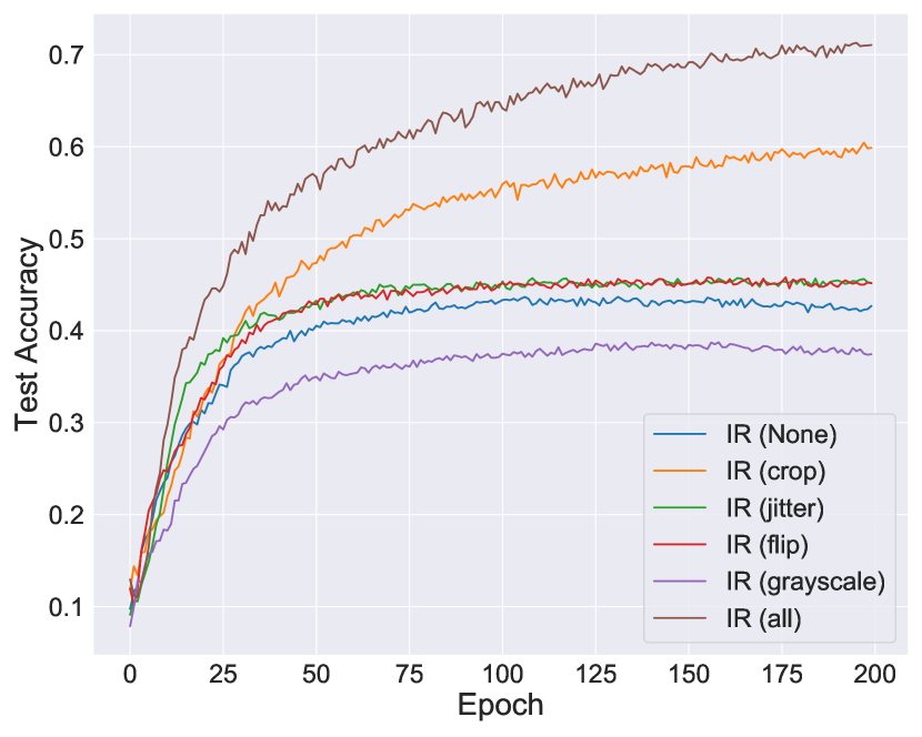
Refer to caption
(a) IR (ImageNet)
Refer to caption
(b) IR (CIFAR10)
Refer to caption
(c) CMC (ImageNet)
Refer to caption
(d) CMC (CIFAR10)
Figure 5: Effect of view set choice on representation quality for IR and CMC on ImageNet. Empty or trivial augmentations (e.g. flipping) lead to poor performance.

Appendix G Properties of a Good View Set

Recall Fig. 1, which measured the quality of different representations learned under different view sets. We continue our analysis to summarize the results with a few properties that differentiate “good” and “bad” views (data augmentation techniques). Property 1 was mentioned in the main text.

Property #1: (Lossy-ness)

We can frame views as a device for information bottleneck that force the encoders to estimate mutual information under missing information: the stronger the bottleneck, the more robust the representation. Further, if the view functions are lossy, then the mutual information (X;X)𝑋𝑋\mathcal{I}(X;X) is not obvious, making the objective nontrivial. Some evidence of this as a desirable property can be seen in Fig. 1: lossless view functions (such as horizontal flipping or none at all) result in poor representations where as more lossy view functions (such as cropping and noise addition) form much stronger representations than lossless and less lossy view functions (e.g. grayscale).

Property #2: (Completeness)

Different views should differ in the information they contain (otherwise the objective is again trivial). Consider the training paradigm for IR: every epoch, for a given x𝑥x, we must choose a random view. In the limit, this paradigm would amortize the parameters of the encoders over all views in vxsubscript𝑣𝑥v_{x}. This compounds the amount of information that must be compressed in the encoded representation, encouraging abstraction and invariance. With this interpretation, completeness is important as we want to be invariant to the full spectrum of views — otherwise, the learned representation would contain “holes” along certain transformations that may appear in unseen images. For instance, consider a view set of center crops versus a view set of all random crops.

Property #3: (Uniqueness)

Given an image, imagine we scramble all pixels to random values. This would clearly make it difficult for the witness function to properly access similarity (and be maximally lossy) but so much so that no meaningful representation can be learned. To avoid this, we demand the view set of a datum to be unique to that datum alone. In other words, the elements of view set vxsubscript𝑣𝑥v_{x} for a data point x𝑥x should not appear in the view set vysubscript𝑣𝑦v_{y} for any y𝑦y. For instance, cropping an image or adding color jitter does not fully obscur the identity of the original image.

Property #4: (Consistency)

For a datum x𝑥x, a view v(x,a)𝑣𝑥𝑎v(x,a) for any a𝒜𝑎𝒜a\in\mathcal{A} must be in the same domain as x𝑥x. For instance, the view of an image cannot be a piece of text. In this sense, we can consider x𝑥x to be a priviledged view (of itself). Because amortizing over views increases the generalization capability of our encoders to elements of vxsubscript𝑣𝑥v_{x} (and since x𝑥x has membership in vxsubscript𝑣𝑥v_{x}), we expect amortization to result in a good representation for the priviledged view x𝑥x. The same-domain assumption is worth highlighting: if we were to choose views of a different dimensionality or modality, we would not be able to encode (untransformed) images from a test set into our representation.

A Second Toy Example

To showcase these properties, consider two interweaved spirals, one spinning clockwise and one counter-clockwise, composed of 2D coordinates: (cx,cy)subscript𝑐𝑥subscript𝑐𝑦(c_{x},c_{y}). Define the elements of the view set vxsubscript𝑣𝑥v_{x} for x𝑥x as (cx+εx,cy+εy)subscript𝑐𝑥subscript𝜀𝑥subscript𝑐𝑦subscript𝜀𝑦(c_{x}+\varepsilon_{x},c_{y}+\varepsilon_{y}) where εx,εyU(0,η)similar-tosubscript𝜀𝑥subscript𝜀𝑦𝑈0𝜂\varepsilon_{x},\varepsilon_{y}\sim U(0,\eta). We vary η𝜂\eta from 0 (only the priviledged view) to 5 (every point possible in the domain).
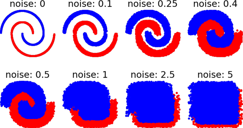
Refer to caption
(a) Sampled Views
Refer to caption
(b) 2D Repr.
Refer to caption
(c) InfoNCE Loss
Refer to caption
(d) Test Acc.
Figure 6: Consider points along two intertwined spirals. (a) We vary the amount of noise added to the points. (b) We visualize the learned 2D representation. (c) Training losses over time. With more noise, MI is lower. (d) The transfer task is to predict which spiral a point belongs to.

Consider the transfer task of predicting which spiral each point belongs to (using logistic regression on the representations). Thus, the information required to disentangle the spirals must be linearly separable in the representations. From Fig. 6, we see that with η=0𝜂0\eta=0 (lossless views), we can maximize MI (low training loss) but the transfer accuracy is near chance. As noise approaches 0.4 (lossy and unique), we find steady improvements to accuracy. From Fig. 6b, only η=0.4𝜂0.4\eta=0.4 has a (mostly) linear separation. However, as noise surpasses 0.4 (and views lose uniqueness), transfer accuracy recedes to chance. These results exemplify the importance of lossy-ness and uniqueness.

Training Details

The encoders are 5-layer MLPs with 128 hidden dimensions and map inputs x𝑥x to a 2D representation. We use 4096 negative samples drawn from the training dataset to optimize InfoNCE with SGD using momentum 0.9, weight decay 1e-5, batch size 128, and learning rate 0.03 for 10k iterations. The memory bank update parameter α𝛼\alpha is set to 0.50.50.5 with a temperature of 0.070.070.07. The double spiral dataset contains 10k points contained within a 2D box of [2,2]2superscript222[-2,2]^{2}.

Refer to caption
(a) Witness (ImageNet)
Refer to caption
(b) Witness (CIFAR)
Refer to caption
(c) Stability (ImageNet)
Refer to caption
(d) Stability (CIFAR)
Refer to caption
(e) α𝛼\alpha+IR (ImageNet)
Refer to caption
(f) α𝛼\alpha+LA (ImageNet)
Refer to caption
(g) α𝛼\alpha+IR (CIFAR)
Refer to caption
(h) α𝛼\alpha+CMC (CIFAR)
Figure 7: Nearest neighbor classification accuracy for various experiments: (a, b) compare different architectures for fθ(x,y)subscript𝑓𝜃𝑥𝑦f_{\theta}(x,y); (c, d) compare the original IR objective with InfoNCE in stability; (e-h) compare different update parameters α𝛼\alpha for the memory bank of IR, LA, and CMC.

Appendix H Additional Results

Learning curves

Fig. 8 show the learning curves comparing IR, BALL, ANN, and LA on ImageNet and CIFAR10. The y-axis plots the nearest neighbor classification accuracy.
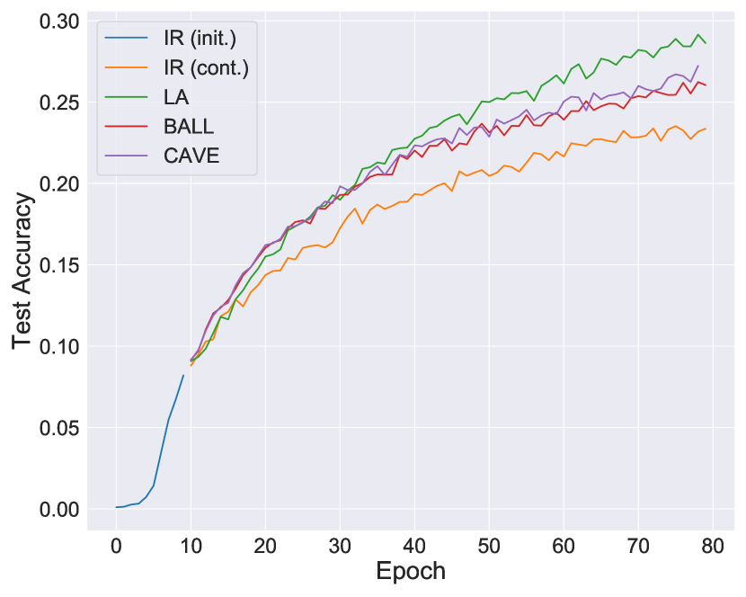
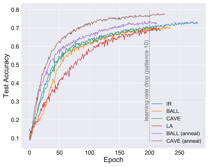
Refer to caption
(a) ImageNet (IR)
Refer to caption
(b) CIFAR10 (IR)
Refer to caption
(c) ImageNet (CMC)
Refer to caption
(d) CIFAR10 (CMC)
Figure 8: Nearest neighbor (NN) classification accuracy throughout training: (a,b) show the IR family of models on ImageNet and CIFAR10; (c,d) show similar results for the CMC family.

Additional COCO Mask R-CNN Results

In the main text, Table 2 show object detection and segmentation results on COCO using the representations learned by various contrastive algorithms. We used a fixed backbone with a feature pyramid network. Table 4 show a similar set of results without a feature pyramid (as is also done in  [6] ). We find the same patterns: that is, annealed Annulus Discrimination outperforms all other models.

Table 4: COCO: Mask R-CNN, R18-C4, 1x schedule
Model APbbbb{}^{\text{bb}} APbb50superscriptsubscriptabsent50bb{}_{50}^{\text{bb}} APbb75superscriptsubscriptabsent75bb{}_{75}^{\text{bb}} APmkmk{}^{\text{mk}} APmk50superscriptsubscriptabsent50mk{}_{50}^{\text{mk}} APmk75superscriptsubscriptabsent75mk{}_{75}^{\text{mk}}
IR 6.16.16.1 13.913.913.9 4.44.44.4 6.06.06.0 12.712.712.7 5.15.15.1
BALL 6.36.36.3 14.314.314.3 4.94.94.9 6.46.46.4 13.213.213.2 5.65.65.6
ANNkmeanskmeans{}^{\text{kmeans}} 6.76.76.7 14.814.814.8 5.35.35.3 6.76.76.7 13.913.913.9 5.95.95.9
LA 7.47.47.4 16.116.116.1 5.75.75.7 7.47.47.4 15.215.215.2 6.46.46.4
BALLannealanneal{}^{\text{anneal}} 7.27.27.2 15.515.515.5 5.65.65.6 7.37.37.3 14.414.414.4 6.26.26.2
ANN+annealkmeanssubscriptsuperscriptabsentkmeans+anneal{}^{\text{kmeans}}_{\text{+anneal}} 7.77.7\mathbf{7.7} 16.516.5\mathbf{16.5} 6.06.0\mathbf{6.0} 7.87.8\mathbf{7.8} 15.515.5\mathbf{15.5} 6.76.7\mathbf{6.7}

Additional CIFAR10 Results

Due to a lack of space, in the main text we only reported Top 1 accuracies for the CIFAR10 dataset. Here we report the full table with Top 5. See Table 5.

Model Top1 Top5 Model Top1 Top5
IR [20] 64.3 95.9 CMC [17] 72.1 97.3
IRncence{}^{\text{nce}} 81.2 98.9 CMCncence{}^{\text{nce}} 85.6 99.4
LA [21] / BALLk-neighk-neigh{}^{\text{k-neigh}} 81.8 99.1 - - -
LAncence{}^{\text{nce}} 82.3 99.1 - - -
BALL 81.4 99.0 BALLLabLab{}^{\textup{Lab}} 85.7 99.5
BALLannealanneal{}^{\textup{anneal}} 82.1 99.1 BALLLab+annealLab+anneal{}^{\textup{Lab+anneal}} 86.8 99.5
BALLs-neighs-neigh{}^{\textup{s-neigh}} 75.1 95.9 BALLLab+s-neighLab+s-neigh{}^{\textup{Lab+s-neigh}} 63.3 94.5
BALLs-neigh+anneals-neigh+anneal{}^{\textup{s-neigh+anneal}} 84.8 99.3 BALLLab+s-neigh+annealLab+s-neigh+anneal{}^{\textup{Lab+s-neigh+anneal}} 87.0 99.4
CAVE 81.4 99.0 CAVELabLab{}^{\textup{Lab}} 86.1 99.5
CAVEannealanneal{}^{\textup{anneal}} 84.8 99.3 CAVELab+annealLab+anneal{}^{\textup{Lab+anneal}} 87.8 99.5
RING 84.7 99.3 RINGLabLab{}^{\textup{Lab}} 87.3 99.4
RINGs-neighs-neigh{}^{\textup{s-neigh}} 76.6 98.6 RINGLab+s-neighLab+s-neigh{}^{\textup{Lab+s-neigh}} 68.0 95.7
RINGannealanneal{}^{\textup{anneal}} 85.2 99.3 RINGLab+annealLab+anneal{}^{\textup{Lab+anneal}} 87.6 99.5
RINGs-neigh+anneals-neigh+anneal{}^{\textup{s-neigh+anneal}} 85.5 99.4 RINGLab+s-neigh+annealLab+s-neigh+anneal{}^{\textup{Lab+s-neigh+anneal}} 87.8 99.5
Table 5: CIFAR10 Transfer Accuracy

Appendix I Additional Discussion

We discuss a few minor points regarding MI and contrastive learning not included in the main text. We also include some additional figures in Fig. 7 for memory bank experiments.
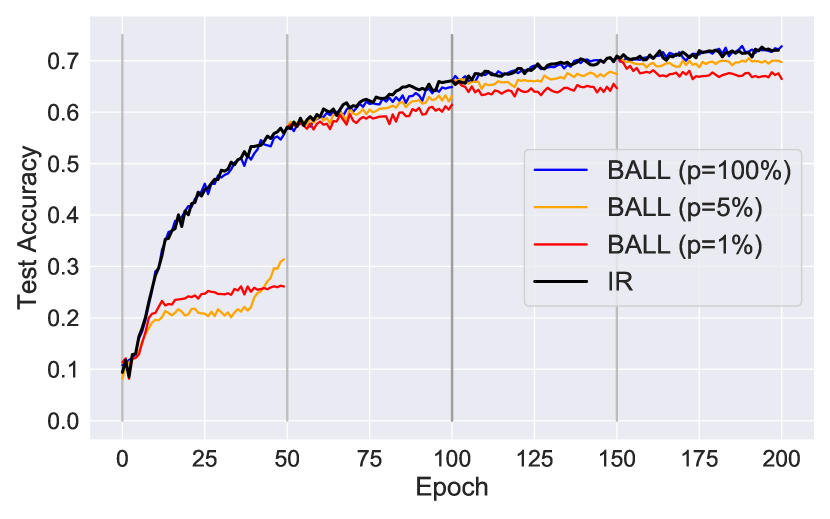
Refer to caption
(a) 100 negatives
Refer to caption
(b) 1024 negatives
Refer to caption
(c) 4096 negatives
Figure 9: Relationship between the total number of negative samples drawn and its distribution: (a,b ,c) show the nearest neighbor classification accuracy when using various values for τ𝜏\tau to define qτsubscript𝑞𝜏q_{\tau}.
Refer to caption
(a) Imagenet (IR)
Refer to caption
(b) CIFAR10 (IR)
Figure 10: Relationship between nearest neighbor classification accuracy and temperature.

The witness function should be under-parameterized.

Since fθ(x,y)subscript𝑓𝜃𝑥𝑦f_{\theta}(x,y) encodes x𝑥x and y𝑦y independently before the dot product, the encoders bear the near-full burden of estimating mutual information. However, could we parameterize fθsubscript𝑓𝜃f_{\theta} more heavily (e.g. perceptron)? Consider the alternative design: fθ,ψ(x,y)=hψ(gθ(x),gθ(y))subscript𝑓𝜃𝜓𝑥𝑦subscript𝜓subscript𝑔𝜃𝑥subscript𝑔𝜃𝑦f_{\theta,\psi}(x,y)=h_{\psi}(g_{\theta}(x),g_{\theta}(y)) where hψsubscript𝜓h_{\psi} is a neural network. At one extreme, gθsubscript𝑔𝜃g_{\theta} and gθsubscript𝑔𝜃g_{\theta} mimic identity functions whereas hψsubscript𝜓h_{\psi} assumes the burden of learning. Representations learned in this setting should prove far less useful. To test this hypothesis, we compare the following designs: (1) a dot product gθ(x)Tgθ(y)subscript𝑔𝜃superscript𝑥𝑇subscript𝑔𝜃𝑦g_{\theta}(x)^{T}g_{\theta}(y); (2) a bilinear transform gθ(x)TWgθ(y)subscript𝑔𝜃superscript𝑥𝑇𝑊subscript𝑔𝜃𝑦g_{\theta}(x)^{T}Wg_{\theta}(y); (3) concatenate gθT(x)superscriptsubscript𝑔𝜃𝑇𝑥g_{\theta}^{T}(x) and gθ(y)subscript𝑔𝜃𝑦g_{\theta}(y) and pass it into a linear layer projecting to 1 dimension; (4,5) concatenate gθT(x)superscriptsubscript𝑔𝜃𝑇𝑥g_{\theta}^{T}(x) and gθ(y)subscript𝑔𝜃𝑦g_{\theta}(y) and pass it through a series of nonlinear layers with 128 hidden nodes before projecting to 1 dimension. In order from (1) to (5), the models increase in expressivity. Fig. 7a and b show classification performance on ImageNet and CIFAR10. We find that a more expressive hψsubscript𝜓h_{\psi} results in lower accuracy, symbolizing a weaker representation. We highlight that these experiments differ from [1] where the authors found fθ,ψ(x,y)=(hψgθ)(x)T(hψgθ)(y)subscript𝑓𝜃𝜓𝑥𝑦subscript𝜓subscript𝑔𝜃superscript𝑥𝑇subscript𝜓subscript𝑔𝜃𝑦f_{\theta,\psi}(x,y)=(h_{\psi}\circ g_{\theta})(x)^{T}(h_{\psi}\circ g_{\theta})(y) to improve performance.

Harder negative samples are not always good.

In Fig. 8 and Table 2, we see that slowly increasing the threshold τ𝜏\tau significantly improves performance (see BALLannealanneal{}^{\text{anneal}}/CAVEannealanneal{}^{\text{anneal}}). This implies that using harder negative samples may not be beneficial at all points in training. Early in training, it could that difficult negatives bias towards a local optima. To test this, we can train BALL models with varied τ𝜏\tau whose parameters are initialized with a IR model at different points of training (e.g. epoch 1 versus epoch 100). Fig. 9 shows exactly this, additionally varying the number of total negatives drawn from 100 to 4096. Recall from the first toy experiment that a smaller percentage p𝑝p represents a larger τ𝜏\tau (with p=100%𝑝percent100p=100\% equaling IR). We make two observations: First, at the beginning of training, difficult negatives hurt the representation. Second, with too few samples, difficult negatives are too close to the current image, stunting training. But with too many samples, difficult negatives are “drowned out” by others. If we balance the difficulty of the negatives with the number of samples, we find improved performance with larger τ𝜏\tau (see Fig. 9b). In summary, always using harder negative samples is not a bulletproof strategy. In practice, we find slowly introducing them throughout training to work well.

The temperature parameter is important.

In simplifying contrastive learning, we might wonder if we could remove the temperature parameter ω𝜔\omega. Fig. 10 suggests that tuning ω𝜔\omega is important for at least the speed of convergence. We find the best ω𝜔\omega to be dataset dependent.