The clustering of LRGs in the DECaLS DR8 footprint: distance constraints from baryon acoustic oscillations using photometric redshifts

Abstract

A photometric redshift sample of Luminous Red Galaxies (hereafter LRGs) obtained from The DECam Legacy Survey (DECaLS) is analysed to probe cosmic distances by exploiting the wedge approach of the two-point correlation function. Although the cosmological information is highly contaminated by the uncertainties existing in the photometric redshifts from the galaxy map, an angular diameter distance can be probed at the perpendicular configuration in which the measured correlation function is minimally contaminated. An ensemble of wedged correlation functions selected up to a given threshold based on having the least contamination was studied in the previous work (Sridhar & Song, 2019) using simulations, and the extracted cosmological information was unbiased within this threshold. We apply the same methodology for analysing the LRG sample from DECaLS which will provide the optical imaging for targeting two-thirds of the DESI footprint and measure the angular diameter distances at $z=0.69$ and $z=0.87$ to be $D_{A}(0.697)=(1499\pm 77\,\mathrm{Mpc})(r_{d}/r_{d,fid})$ and $D_{A}(0.874)=(1680\pm 109\,\mathrm{Mpc})(r_{d}/r_{d,fid})$ with a fractional error of 5.14% and 6.48% respectively. We obtain a value of $H_{0}=67.59\pm 5.52$ km/s/Mpc which supports the $H_{0}$ measured by all other BAO results and is consistent with $\Lambda$CDM model.

1 Introduction

Measuring the expansion history of the Universe is of paramount importance in the field of modern cosmology. It can be revealed by diverse cosmic distance measures in tomographic redshift space, such as cosmic parallax (Benedict et al., 1999), standard candles (Fernie, 1969) or standard rulers (Eisenstein et al., 1998, 2005). To date the best constraints come from the distance-redshift relation and imply that the expansion rate has changed from a decelerating phase to an accelerated one (Riess et al., 1998; Perlmutter et al., 1999). As most ongoing observations support the $\Lambda$CDM model with the presence of the cosmological constant, but to confirm it with high precision or to possibly find any deviation from it still remains an interesting observational mission. One of the most robust methods for measuring distance-redshift relation is to use the baryon acoustic oscillation feature that is observed as a bump in the two-point correlation function or as wiggles in the power spectrum. The tension between gravitational infall and radiative pressure caused by the baryon-photon fluid in the early Universe gave rise to an acoustic peak structure which was imprinted on the last-scattering surface (hereafter BAO) (Peebles & Yu, 1970). The BAO feature has been measured through the correlation function (Eisenstein et al., 2005), and the most successful measurements in the clustering of large-scale structure at low redshifts have been obtained using data from SDSS (Eisenstein et al., 2005; Estrada et al., 2009; Padmanabhan et al., 2012; Hong et al., 2012; Veropalumbo et al., 2014, 2016; Alam et al., 2017). The Dark Energy Spectroscopic Instrument (DESI) is an upcoming survey (DESI Collaboration et al., 2016) which will be launched to probe the earlier expansion history with greater precision using spectroscopic redshifts. However, the photometric footprint for DESI has already been completed by the Legacy Imaging Surveys (Dey et al., 2018). Photometric surveys provide more observed galaxies compared to a spectroscopic survey even at deeper redshifts (Euclid Collaboration et al., 2019), but the uncertainty on the redshift obtained from photometric surveys is larger compared to the uncertainty on the redshift obtained from spectroscopic surveys. Although these photometric redshifts are measured with a much poorer resolution and an unpredictable damping of clustering at small scales and a smearing of the BAO peak is caused by the photo-z uncertainty (Estrada et al., 2009), possible BAO signatures that have not been washed-out by the redshift uncertainty might still be present.

We investigate the optimised methodology to extract the cosmic distance information from the photometric datasets and provide a precursor of cosmic distance information which will be revealed by the follow up spectroscopy experiment much later on. We apply the wedge approach (Kazin et al., 2013; Sánchez et al., 2013, 2014; Sabiu & Song, 2016; Ross et al., 2017; Sánchez et al., 2017; Sridhar & Song, 2019) to probe the uncontaminated BAO feature by binning the angular direction from the perpendicular to radial directions, and recover the residual BAO peak that has survived and get constraints on the angular diameter distance $D_{A}$ and $H^{-1}$. It has also been shown recently by Ross et al. (2017) that the statistics obtained using wedge correlation function are about 6% more accurate compared to the angular correlation function. Thus, using $\xi_{w}(s,\mu)\,$not only adds more information compared to $w(\theta)$, but also overcomes the above disadvantages.

Recently, some improved methodologies have measured the Hubble constant in great precision, which reveal a tension among measurements. This tension draws attention to the community as a possible presence of new physics or unknown systematic uncertainties that need to be fixed. The Hubble constant is indirectly measured by the highest resolution cosmic microwave background maps provided by the Planck satellite experiment (The Planck Collaboration, 2006) and they find it to be $H_{0}=67.4\pm 0.5{\rm\,km/s/Mpc}$ (Planck Collaboration et al., 2018). The Hubble constant can also be directly probed by classical distance ladder using type Ia Supernovae samples (Scolnic et al., 2019). The latest value from Riess et al. (2019) give us a constraint of $H_{0}=74.03\pm 1.42{\rm\,km/s/Mpc}$ with a few percent marginal error. Both efforts leaves a huge discrepancy in the $H_{0}$ measurement, with the values being 4$\sigma$ apart, which needs to be resolved.

While the current analyses of most cosmological observations at low redshift support the $H_{0}$ measured by Planck, next generation survey programs such as DESI will be launched in the near future. DESI will probe the earlier expansion history with greater precision using spectroscopic redshifts. However, by using the DECaLS data, which provides us constraints on the angular diameter distance and by using the information of the sound horizon from Planck, we get constraints on $H_{0}$. Our analyses uses a fiducial cosmological model with the following parameters: $\Omega_{m}=0.31$, $\Omega_{b}=0.049$, $h\equiv H_{0}/(100\,\mathrm{kms^{-1}Mpc^{-1}})=0.676$, $n_{s}=0.96$ and $\sigma_{8}=0.8$. The paper is organised as follows. In Section 2, we describe the DECaLS DR8 data data including the magnitude cuts we employ for our sample. Section 3 describes the clustering measurements and the fitting procedure used. We present our cosmic distance constraints obtained in Section 4 and discuss our overall results and conclusions in Section 5.

2 The Data

In this section, we describe the DESI Legacy Imaging Survey DR8 data used in this paper along with the Dark Sky simulation data used for testing and validating our results.

2.1 DECaLS DR8 data

The DESI Legacy Imaging Surveys will provide the target catalogue for the upcoming DESI survey. One among the 3 imaging projects conducted for the Legacy Survey is DECaLS (Dey et al., 2018) which covers the South Galactic Cap region at DEC $\leq$ 34^∘. The data makes use of three optical bands (g,r, and z) to a depth of at least $g=24.0$, $r=23.4$ and $z=22.5$, which is 1-2 magnitude deeper than SDSS. We use the DECaLS data from the Legacy Surveys eighth data release (DR8), which is the first release to include images and catalogues from all three of the Legacy Surveys in a single release. The Legacy Surveys also processed some of the imaging data from the Dark Energy Survey (DES, The Dark Energy Survey Collaboration 2005), and we include the DES imaging with DEC $\geq$ -30^∘ in our analysis. In addition to the optical imaging, 4 years of Wide-Field Infrared Survey Explorer (WISE) (Wright et al., 2010; Meisner et al., 2017) data in the W1 and W2 bands are also included, which provide additional colour information.

For the parent LRG sample in this study, we use a non-stellar cut of $(z-\mathrm{W}1)-0.8*(r-z)>-0.6$, a faint limit of $z<20.41$, a colour cut of $0.75<(r-z)<2.45$ and a sliding magnitude-color cut of $(z-17.18)/2<(r-z)$. These selection cuts are motivated by the current DESI LRG target selection cuts (DESI Collaboration et al., 2016).

We also apply masks to get the final footprint for our parent sample using the “MASKBITS” column in the DR8 catalog . Objects (and randoms) with following bits are removed: 1 (Tycho-2 and GAIA bright stars), 8 (WISE W1 bright stars), 9 (WISE W2 bright stars), 11 (fainter GAIA stars), 12 (large galaxies) and 13 (globular clusters). Imaging datasets often suffer from systematic effects, and one such major contribution towards the systematic contamination comes from correlation with stellar density (Rezaie et al., 2019). A more detailed test on this effect on the large-scale structure correlation is explained in Section A.

After applying the magnitude cuts and masking scheme, we use random forest-based (Breiman, 2001) photo-z’s from Zhou et al. (2020) to obtain the final photometric redshifts. The dispersion on the redshift is usually approximated by,

$$\sigma_{z}\equiv\sigma_{0}\times(1+z_{true}),$$ (1)

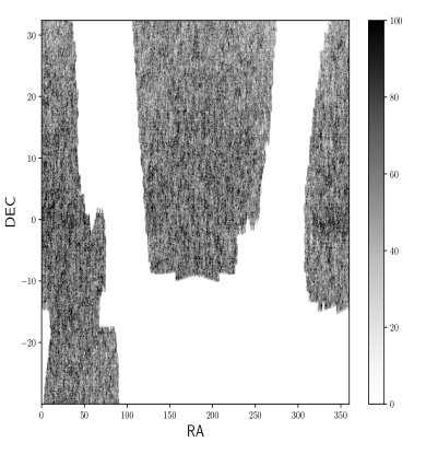
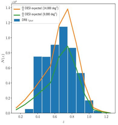
where $\sigma_{0}$ denotes the dispersion at redshift $z=0$ and $z_{true}$ is the true redshift or the spectroscopic redshift. The mean redshift uncertainty for the DECaLS DR8 sample within the range $0.3<z_{phot}<1.2$ is $\sigma_{0}=0.0264$. The angular distribution of the parent LRG sample after applying the masking and selection cuts is plotted in the left panel of Figure 1, with higher density regions denoted by a darker shade. The redshift distribution of the parent sample within the range $0.3<z_{phot}<1.2$ is plotted as blue filled histogram in the right panel of Figure 1. For comparison, we also overplot the forecasted $dN/dz$ LRG redshift distribution from DESI for a sky coverage of 9000 deg² (given by the green solid line) and 14000 deg² (given by the orange solid line). The DECaLS DR8 sample has a sky coverage of $\approx$ 9500 deg², which more than two-thirds of the 14,000 deg² DESI footprint.

2.2 Dark Sky simulation data

In order to test and validate the results we obtain, we also need to analyse the clustering from a realistic mock catalogue based on numerical simulations that calculate the non-linear evolution of structure and predict the dependence of survey observables on cosmological parameters. We use the publicly available Dark Sky simulation set as described in Skillman et al. (2014) for this purpose. The simulation has been generated using particle numbers varying from 2048³ to 10240³ and in a comoving cosmological volume varying from $100$h^-1Mpc to $8$h^-1Gpc box on a side. The objects have been placed in the simulation using a simple (time-evolving) Halo Occupation Distribution (HOD) assuming spherical, Navarro-Frenk-White (Navarro et al., 1996), halos for the satellite. To identify dark matter halos and substructures, the ROCKSTAR halo finder (Behroozi et al., 2013) has been used. The halo-finding approach is based on an adaptive hierarchical refinement of friends-of-friends groups in both position and velocity. From the set of simulations (with varying particle numbers), we make use of the ds14_a simulation which has 10240³ particles and a particle mass of $3.9\times 10^{10}h^{-1}M_{\odot}$. These specific mocks contain only RA, DEC and true redshift information for objects pre-identified to be LRGs and do not contain color or luminosity information.

Figure 1: Left panel: The angular distribution of the LRGs from the DECaLS DR8 photometric sample after applying the masking scheme and selection cuts. The density variations are shown using a normalised “grayscale” colormap, with darker regions denoting the high dense regions. Right panel: The photometric redshift distribution of the DECaLS DR8 parent sample (blue filled histogram) obtained using the random forest method. The green and orange solid lines are the forecasted $dN/dz$ for LRG galaxies achievable by DESI (DESI Collaboration et al., 2016) for a sky coverage of 9000 and 14000 deg² respectively.

To validate our results on photometric redshifts, we generate a set of photo-z’s using the true redshift information available. In reality, the statistical nature of the photo-z error is more complicated to be specified with any known distribution function, but it is assumed that the error propagation of photo-z uncertainty into cosmological information is mainly caused by the dispersion length (Arnalte-Mur et al., 2009). Thus a simple Gaussian function of statistical distribution is chosen for generating the photo-z uncertainty distribution, and we apply the photo-z error dispersion $\sigma_{z}$ as defined in Eq. 1 (a more detailed description is given in Section 3.3). In reality, the precision is dependent on many factors such as magnitude and spectral type, but here only the redshift factor is counted in Eq. 1 in which the coherent statistical property determined only by $z$ is applied for all types of galaxies in the simulation.

Table 1 summarises the number density information from both the DECaLS data and the Dark Sky data for the entire redshift range and for the two redshift cuts used in this paper. It can be seen that the number density in all the three redshift ranges for the mock is smaller than the DECaLS sample. Thus, the comparison in the clustering between the two samples should only be looked into as a consistency check rather than a precise validation of our results.

	Redshift range	$N_{gals}$	$V$ (Gpc3)	$\sigma_{0}$
	$0.3<z_{phot}<1.2$	5193078	7.64	0.0263
DECaLS	$0.6<z_{phot}<0.8$	2083394	1.74	0.0262
	$0.8<z_{phot}<1.0$	1074916	2.25	0.0352
	$0.3<z_{phot}<1.2$	2781896	6.51	0.0284
Dark Sky	$0.6<z_{phot}<0.8$	1271670	1.65	0.0282
	$0.8<z_{phot}<1.0$	560749	2.16	0.0341
EZmock	$0.6<z_{phot}<0.8$	2058906	1.65	0.0263
	$0.8<z_{phot}<1.0$	963673	2.16	0.0342

Table 1: Number of LRGs, volume for the sample within the range $0.3<z_{phot}<1.2$ (also for the two redshift cut samples used in this paper) and the mean redshift uncertainty within the redshift range ($\sigma_{0}$) for the DECaLS, Dark Sky mock and the EZmock sample (average values from the realisations). The $N_{gals}$ quoted is the total number of LRGs used in the large-scale clustering analysis.

2.3 EZmock simulation data for covariance matrix

To compute the error on $\xi_{w}(s,\mu_{i})$, we make use of 100 EZmock (Chuang et al., 2015) simulations all of which have the DESI expected sky coverage. To match the DECaLS DR8 footprint, we cut the EZmock samples within $-30^{\circ}<\mathrm{DEC}<$ 34^∘. The EZmock sample after the DEC cut has an area of $\approx$ 9300 deg², which is similar to the are of the DECaLS DR8 parent sample that we use in this paper. The mocks contain RA, DEC, $z_{cosmo}$ and $dz_{rsd}$ information. Thus, we need to generate photometric redshifts for the mocks so that they can be used to obtain the covariance matrix, and we do so using the Gaussian approximation following Eq. 1.

To generate the photo-z’s for our sample, we obtain $\sigma_{z}$’s randomly from the parent DECaLS sample, but by restricting to galaxies of similar redshifts that are within a redshift range of $\pm$0.1 $z_{phot}$ which ensures that the dependence of errors on redshift is included. For example, for $N$ number of EZmock galaxies that are within $0.6<z_{cosmo}<0.7$, $N$ $\sigma_{z}$’s from the DECaLS data within $0.6<z_{phot}<0.7$ are randomly selected. This process is repeated over the entire redshift range. Once we generate the photo-z’s, they are diluted according to the DECaLS $N(z)$ to make sure that they are consistent. The number of galaxies, volume within the redshift range and the $\sigma_{0}$ for the two redshift cuts is mentioned in Table 1. Our detailed analysis comparing the $\xi_{w}(s,\mu)\,$between the EZmock sample and the DECaLS sample are explained in Section B and shown in Figure 8.

3 Methodology

In this paper, we follow the same methodology and formulation that was applied in Sridhar & Song (2019) to simulated photometric galaxy catalogues to get cosmological distance constraints. We explain in detail the clustering measurements obtained from the wedge correlation function and the comparison between the DECaLS and Dark Sky mock data.

3.1 Clustering measurements and fitting procedure

The excess probability of finding two objects relative to a Poisson distribution at volumes $dV_{1}$ and $dV_{2}$ separated by a vector distance r is given by the two-point correlation function $\xi(r)$ (Totsuji & Kihara, 1969; Davis & Peebles, 1983). The galaxy distribution seen in redshift space exhibits an anisotropic feature distorting $\xi(r)$ into $\xi(\sigma,\pi)$ along the line-of-sight (LOS) where $\sigma$ and $\pi$ denote the transverse and radial components of the separation vector r. Acoustic fluctuations of the baryon–radiation plasma of the primordial Universe leaves the signature on the density perturbation of baryons. This standard ruler length scale, set by the acoustic wave, propagates until it is frozen at decoupling epoch to remain in the large scale structure of the Universe. The threshold length scale of the acoustic wave is called the sound horizon, which is given by,

$$r_{d}=\int_{z_{drag}}^{\infty}\frac{c_{s}(z)}{H(z)}dz$$ (2)

where $c_{s}$ is sound speed of the plasma. This scale is imprinted on the correlation function as a peak and is imprinted on the matter power spectrum as a series of waves. Assuming standard matter and radiation content in the Universe, the Planck Collaboration et al. (2018) measurements of the matter and baryon density determine the sound horizon to 0.2%. By measuring the BAO feature using an anisotropic analysis, one can separately measure $D_{A}(z)$ and $H^{-1}(z)$. But adjustments to the cosmological parameters or changes to the pre-recombination energy density can alter the value of $r_{d}$ (Alam et al., 2017). So, the BAO measurements constrain the combinations $D_{A}(z)/r_{d}$, $H^{-1}(z)r_{d}$. The sound horizon for this fiducial model is $r_{d,fid}=147.21$ Mpc as obtained from Planck Collaboration et al. (2018). The scalings of $r_{d}$ with cosmological parameters can be found in detail in Aubourg et al. (2015). The distance constraints quoted in this paper are in units of Mpc and with a scaling factor, e.g., $D_{A}(z)\times(r_{d,fid}/r_{d})$, so that the numbers provided are independent of the fiducial cosmological parameters used.

The Landy & Szalay estimator (hereafter LS) in $(s,\mu)$ coordinates is best suited to calculate the two-point correlation function (Farrow et al., 2015; Sridhar et al., 2017) and extract BAO information from photometric redshift galaxy maps (Sridhar & Song, 2019). The radius to shell $s$ and the observed cosine of the angle the galaxy pair makes with respect to the LOS $\mu$ are given by $s^{2}=\sigma^{2}+\pi^{2}$ and $\mu=\pi/s$ respectively, where $\sigma$ and $\pi$ denote the transverse and radial separation between the galaxy pairs.

It is common practice to separate the random sample distributions into the angular and redshift components separately. We make use of the random catalogue provided in the DR8 data release by the Legacy Survey, which gives us the angular component. These randoms have been downsampled to the surface density of 10000 $/$deg ² and requiring +2 exposures in $g$, $r$ and $z$ bands. The number of objects are usually twice or more than the data catalogue to avoid shot noise effects. In our case the random catalogue has 5 times more objects than the data catalogue. For the redshift component, we extract redshifts randomly from the data catalogue within the chosen redshift range (see Ross et al., 2012, 2017; Veropalumbo et al., 2016; Sridhar & Song, 2019, for more info). The same number of exposure requirements, footprint cuts, and bright star masks are applied on the randoms as used in constructing the LRG sample. We use the publicly available KSTAT (KD-tree Statistics Package) code (Sabiu, 2018) to calculate all our correlation functions.

We pay attention to the usefulness of exploiting the wedge correlation function to separate the radial contamination from the BAO signal imprinted on perpendicular configuration pairs. The wedge correlation function $\xi_{w}$ is given by,

$$\xi_{w}(s,\mu_{i})=\int^{\mu_{i}^{\rm max}}_{\mu_{i}^{\rm min}}d\mu^{\prime}W(\mu^{\prime}:\mu_{\rm cut}=\mu_{i}^{\rm max})\xi(s,\mu^{\prime}),$$ (3)

where $\mu_{i}$ is the mean $\mu$ in each bin (we will refer to the mean value of the $\mu$ bin using $\bar{\mu}$ hereafter), and $\mu_{i}^{\rm min}$ and $\mu_{i}^{\rm max}$ are the minimum and maximum values of $\mu$, and $W$ is a window function within the chosen minimum and maximum limits of $\mu$. Using too many $\mu$ bins will complicate the covariance matrix and by using very few $\mu$ bins we will not be able to separate the error propagation along the LOS clearly (Sabiu & Song, 2016). Thus, we choose 6 bins in the $\mu$ direction with $\Delta\mu=0.17$ between $\mu=0$ and 1 with $\mu\rightarrow$ 0 corresponding to the transverse plane and $\mu\rightarrow$ 1 corresponding to the LOS plane.

In the case of photometric redshift samples, the noise on the pairs increases along the radial configuration and thus causes a smearing of the BAO peak (Estrada et al., 2009). This smearing not only increases with increasing photometric uncertainty but also increases along the LOS for a given $\sigma_{0}$. These noisy pairs can be removed using a cutoff $\bar{\mu}$. It has been shown in Sridhar & Song (2019) that using a cutoff $\bar{\mu}=0.42$ for photometric redshift samples can remove most of the contaminated pairs and thus we use a cutoff $\bar{\mu}=0.42$ in this paper. The empirical model that we use to fit the correlation function and obtain the BAO peak location is similar to the one proposed by Sánchez et al. (2011, 2012) and is given by,

$$\xi_{\rm mod}(s)=B+\left(\frac{s}{s_{0}}\right)^{-\gamma}+\frac{N}{\sqrt{2\pi\sigma^{2}}}\mathrm{exp}\left(-\frac{(s-s_{m})^{2}}{2\sigma^{2}}\right),$$ (4)

where $B$ takes into account a possible negative correlation at very large scales, $s_{0}$ is the correlation length (the scale at which the correlation function $\simeq$ 1) and $\gamma$ denotes the slope. The remaining three parameters, $N$, $\sigma$ and $s_{m}$ are the parameters of the Gaussian function that model the BAO feature and, in particular, $s_{m}$ represents the estimate of the BAO peak position. This empirical model can be used to accurately extract the BAO peak position (Sánchez et al., 2011; Veropalumbo et al., 2016; Sridhar & Song, 2019) when the correlation function is provided.

The likelihood on $s_{m}$ from previous BAO studies is either obtained by using a 1d grid on $s_{m}$ where the $\chi^{2}$ is minimized at each grid point or from the marginalized posterior from a Monte Carlo Markov Chain (MCMC) analysis. In this study, the fitting is performed by applying the MCMC technique (we make use of the emcee Python package (Foreman-Mackey et al., 2013)) , using the full covariance matrix obtained using Eq.7. The fitting parameter space is given by,

$$x_{p}=(B,s_{0},\gamma,N,s_{m},\sigma)$$ (5)

and we place flat, wide priors on all the 6 parameters. For the first three parameters, the range of the priors are $0.0<B<1.0$, $0.0<s_{0}<3.0$ and $0.0<\gamma<3.0$ and for the remaining three parameters of the Gaussian function, the range of the priors are $0.0<N<1.0$, $85.0<s_{m}<130.0$ and $0.0<\sigma<35.0$. Several variations of the range of these priors were tested, especially the range of the prior on $s_{m}$ and $\sigma$. A smaller range for the $s_{m}$ affects posterior distribution and we miss most of the information at high $s(h^{-1}\mathrm{Mpc})$. A similar effect is seen when we use a smaller range for the $\sigma$ prior, which eventually amplifies the BAO peak. We have also tested several ranges within which to perform the fit and we fit the correlation function within the range $30.0<s(h^{-1}\mathrm{Mpc})<130.0$ after experimenting with other ranges. We find that there is a maximum shift of 1% in the BAO peak when we vary the range of the fit. This 1% shift is negligible compared to the error on the BAO peak point we obtain (as discussed in Section 3.3) and thus we believe it is subdominant. The constraints on the BAO peak $s_{m}$ for the wedge correlation function is obtained after fully marginalising all other parameters in $x_{p}$. We adopt a standard likelihood, $\mathscr{L}\propto\mathrm{exp}(-\chi^{2}/2)$ where the function $\chi^{2}$ is defined as,

$$\chi^{2}_{\mu_{i}}(x_{p})=\sum_{s,s^{\prime}}(\xi_{\rm mod}(s)-\xi_{w}(s,\mu_{i}))C^{-1}_{s;s^{\prime}}(\mu_{i})$$

$$(\xi_{\rm mod}(s^{\prime})-\xi_{w}(s,\mu_{i}))$$ (6)

where $\xi_{\rm mod}(s)$ is the model correlation function as given by Eq. 4, $\xi_{w}(s,\mu_{i})$ is the observed correlation function for the $i^{\rm th}$ $\bar{\mu}$ bin and $C^{-1}$ is the inverse covariance matrix.

3.2 Covariance matrix from EZmock samples

A random catalogue that is approximately 20 times the mock data is provided for the EZmock samples, but contains only the angular component (RA,DEC). Since the density of the DECaLS randoms is only 5 times the data catalogue, we dilute the EZmock randoms to the same density to ensure consistency in our results. For the redshift component, we follow the same method of randomly extracting $\sigma_{z}$ from the data catalogue.

We calculate the covariance matrix which is given by,

$$C^{ij}_{w}(\xi^{i}_{w},\xi^{j}_{w})=\frac{1}{N-1}\sum^{N}_{n=1}[\xi^{n}_{w}(\vec{x}_{i})-\overline{\xi}_{w}(\vec{x}_{i})][\xi^{n}_{w}(\vec{x}_{j})-\overline{\xi}_{w}(\vec{x}_{j})],$$ (7)

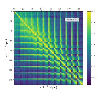
where the total number of simulations is given by $N$. The $\xi^{n}_{w}(\vec{x}_{i})$ represents the value of the wedge correlation function of $i^{th}$ bin of $\vec{x}_{i}$ in the $n^{th}$ realisation, and $\overline{\xi}_{w}(\vec{x}_{i})$ is the mean value of $\xi^{n}_{w}(\vec{x}_{i})$ over all the realisations. Due to the limited number of mock samples (100) that we have, we use 12 bins in $s$. We obtain the correlation matrix as,

$$C_{ij}=\frac{\mathrm{Cov}(\xi_{i},\xi_{j})}{\sqrt{\mathrm{Cov}(\xi_{i},\xi_{i})\mathrm{Cov}(\xi_{j},\xi_{j})}}$$ (8)

which is plotted in Figure 3.

The number of realisations exceeds the number of $(s,\mu)$ bins of 72 bins ($12(s$bins)$\times 6(\mu$bins)), and the inverse of $C_{ij}$ is well defined and thus does not require any de-noising procedures such as singular value decomposition. Additionally, we also count the offset caused by the finite number of realisation (Hartlap et al., 2007) as,

$$C^{-1}=\frac{N_{mocks}-N_{bins}-2}{N_{mocks}-1}\ \hat{C}^{-1}\ ,$$ (9)

where $N_{bins}$ denotes the total number of $i$ bins. As mentioned in Section 3.1, we fit the correlation function within the range $30.0<s(h^{-1}\mathrm{Mpc})<130.0$. Thus, the number of $s$ bins in this range is 9. As the final 3 $\mu$ bins along the LOS do not contain any BAO information, we perform the fitting by ignoring them. Thus, the shape of the matrix is 27$\times$27 and for 100 mock realisations, the factor in Eq. 9 becomes 0.71. Apart from the above correction factor, an additional correction to the inverse covariance matrix is proposed by Percival et al. (2014), which is given by,

$$m_{1}=\frac{1+B(n_{b}-n_{p})}{1+A+B(n_{p}+1)}$$ (10)

where $n_{b}$ is the number of bins used for the two-point correlation measurements, $n_{p}$ is the number of parameters measured and the $A$ and $B$ terms are given by,

$$A=\frac{2}{(n_{s}-n_{b}-1)(n_{s}-n_{b}-4)}$$ (11a)

$$B=\frac{(n_{s}-n_{b}-2)}{(n_{s}-n_{b}-1)(n_{s}-n_{b}-4)}$$ (11b)

where $n_{s}$ is the number of simulations used for the covariance matrix calculations. Applying the square root of this expression to the measured standard deviation should take care of the extra correction. For our binning scheme as mentioned above (with 100 mock realisations), we get $\sqrt{m_{1}}=0.89$ which is significantly smaller than the correction factor we already apply. The BAO peak position $s_{m}$ of the wedge correlation function is found by fitting the phenomenological model by considering full covariance using $C_{ij}$.

Figure 2: The correlation function $\xi_{w}(s,\mu)\,$(multiplied by $s^{2}$) calculated by splitting into wedges of $\mu$ for the $0.6<z_{phot}<0.8$ sample (given by blue dots) and for the $0.8<z_{phot}<1.0$ sample (given by red dots). The first, second and third columns in the figure represent $\bar{\mu}=0.08$, 0.25 and 0.42 bins respectively. The dashed black lines in each plot show the best-fit (maximum likelihood) obtained from the empirical model by applying the MCMC technique. The error bars plotted are the square root of the diagonal elements of the full covariance matrix as mentioned in Eq. 7.

Figure 3: The correlation matrix for the $0.6<z_{phot}<0.8$ sample using 12 bins in $s$ and 6 bins in $\mu$ computed using Eq. 8.

Figure 4: Left panel: The marginalised posterior distribution of the peak point $s_{m}$ obtained from the MCMC analysis using Equation 4 for all the 3 $\mu$ bins in the redshift range $0.6<z_{phot}<0.8$. The covariances between the different $s_{m}$ values is shown in the contour plots and the orange circle encompasses all points within the 1$\sigma$ region. The marginalised distribution for each $s_{m}$ independently is shown in the histograms along the diagonal. Right panel: The same for the $0.8<z_{phot}<1.0$ sample.

3.3 DECaLS and Dark Sky mock acoustic-scale measurements from wedge correlation function

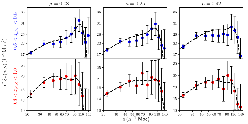
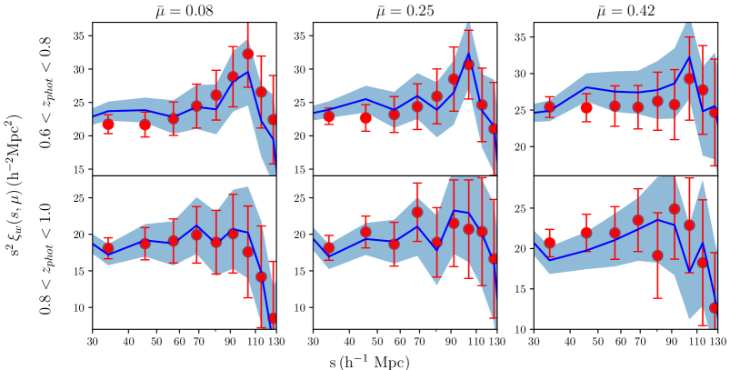
From the parent DECaLS DR8 sample within the redshift range $0.3<z_{phot}<1.2$, we choose two redshift cuts between $0.6<z_{phot}<0.8$ and $0.8<z_{phot}<1.0$ for our analysis. The reason for choosing these two redshift ranges is because the redshift distribution of the sample peaks at $z_{phot}\approx 0.7$ as it can be seen from Figure 1. Thus, we expect to have the maximum number of galaxies around this redshift range. The redshift uncertainty scales with redshift, so we quote the mean values for our two redshift cut samples in Table 1. The wedge correlation functions are calculated using Eq. 3 by using 6 $\mu$ bins of thickness $\Delta\mu=0.17$. The $\xi_{w}(s,\mu_{i})$ calculated from the first three $\mu$ bins for the two redshift samples is shown in Figure 2. We fit $\xi_{w}(s,\mu)\,$using Eq. 4 by following the MCMC procedure described in Section 3.1 and the values of the BAO peak $s_{m}$ from the fit is provided in Table 2.

One can observe that for both the redshift samples, the BAO signal is diluted as $\mu$ increases, and is also more clearly visible for the first redshift sample compared to the second redshift sample. This is due to the fact that the photometric redshift errors scale proportional to $\sigma_{0}\times(1+z)$, and thus the isotropy along the LOS is destroyed more strongly for the high redshift sample compared to the low redshift one. It can also be seen from Table 2 that for the same reason, the BAO peak appears at greater $s$ at greater $\mu$ for both the redshift samples. This trend is more strongly observed for the first redshift sample with $s_{m}$ increasing from 109.7 h^-1Mpc to 111.0 h^-1Mpc from $\bar{\mu}=0.08$ to 0.42. The errors on $s_{m}$ gradually increase with increasing $\bar{\mu}$ as expected.

For both the redshift ranges and all the 3 $\bar{\mu}$ bins used, we fit the correlation function within the range $30.0<s(h^{-1}\mathrm{Mpc})<130.0$. When using log binning instead of linear binning we note that the BAO peak results slightly shift to higher values. However, the effect is of the order of 1%, which is well below the estimated accuracy of the BAO peak position, which is between 4-10% for our samples. We use the $\chi^{2}/dof$ goodness of fit indicator to validate the performance of our empirical model to fit the correlation function. The overall fit to the $0.6<z_{phot}<0.8$ sample yields a $\chi^{2}/dof$ = 12/9 ,including all cross-covariance between $\bar{\mu}$ bins. We obtain a $\chi^{2}/dof$ = 15/9 for the $0.8<z_{phot}<1.0$ sample.

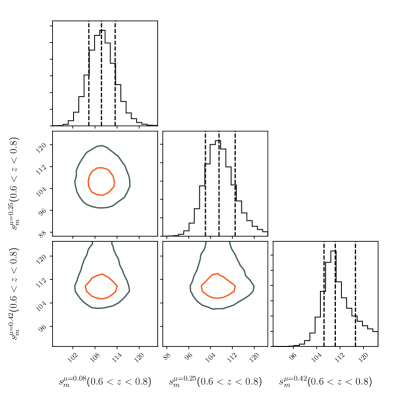
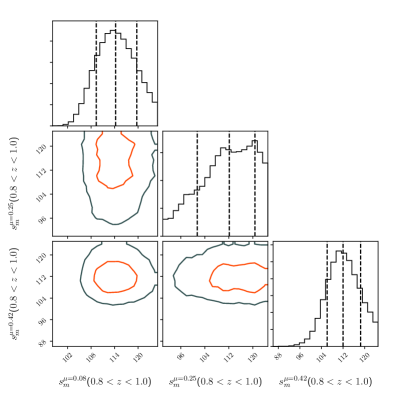
It has been shown from previous studies (Ross et al., 2012, 2017) that data from the different $\mu$ bins is expected to be correlated and that the results from splitting the clustering by $\mu$ show a slight decrease in the BAO information content with increasing $\mu$. Thus, we perform the fit using the full data vector including all the $\mu$ bins. By performing the fit using the full covariance matrix, we make sure that the correlations between the different $\mu$ bins that exist are taken into account. The one and two dimensional projections of the posterior probability distribution of the $s_{m}$ parameter from the MCMC chains for the two redshift samples is shown in Figure 4. The marginalized distribution for each $s_{m}$ value from each $\bar{\mu}$ bin is shown independently in the histograms along the diagonal and the marginalized two dimensional distributions in the other panels. We find that the correlation between the $s_{m}$ values obtained at the different $\mu$ bins for both the redshift samples to be minimal.

Redshift range	$\bar{\mu}$ bin	$s_{m}$ (h-1Mpc)
	0.08	$109.7^{+3.6}_{-3.4}$
$0.6<z_{phot}<0.8$	0.25	$107.1^{+5.8}_{-5.0}$
	0.42	$111.0^{+7.8}_{-4.3}$
	0.08	$111.2^{+5.3}_{-4.9}$
$0.8<z_{phot}<1.0$	0.25	$111.4^{+9.1}_{-9.4}$
	0.42	$112.0^{+6.4}_{-5.8}$

Table 2: Results of fitting the correlation function (plotted using the dotted lines in Figure 2) for the two redshift samples and in the 3 $\bar{\mu}$ bins using Eq. 4. The $s_{m}$ is the BAO peak point obtained from the fit and the units are in h^-1Mpc.

For validating our clustering results obtained on the DECaLS data, we use the LRGs from the Dark Sky mock catalogue. For mimicking the photometric redshifts from the DECaLS data, we use the same procedure followed for generating photo-z’s for our EZmock sample. We obtain $\sigma_{z}$’s randomly from the parent DECaLS sample, but by restricting to galaxies of similar redshifts. To compare the correlation function results obtained from the two redshift samples of the DECaLS catalogue, we compute $\xi_{w}(s,\mu)\,$from the Dark Sky photometric redshift catalogues with the same redshift cuts and use the same binning scheme. We find that by using the true values of $\xi_{w}(s,\mu)\,$for the two photometric redshift samples from the Dark Sky mocks, the amplitudes of $\xi_{w}(s,\mu)\,$do not match with the $\xi_{w}(s,\mu)\,$from the DECaLS data. However, by adding a constant value of 0.0005 and 0.0010 to the $\xi_{w}(s,\mu)\,$obtained from the Dark Sky mocks for the $0.6<z_{phot}<0.8$ and $0.8<z_{phot}<1.0$ samples, we see that the amplitudes match well. The results are presented in Figure 5.

There are two key features that we are interested in when comparing the data and the mock catalogue. One is the amplitude of $\xi_{w}(s,\mu)\,$and the other is the location of the BAO peak. We find that the amplitude of the clustering measurements from the Dark Sky mock catalogue (given by solid blue line) match with the amplitude of the clustering measurements from the DECaLS sample (given by the red scatter points) for both the redshift samples in all the 3 $\bar{\mu}$ bins after adding the constant values to our redshift samples as described above. To statistically compare the linear correlation between the two samples, we use the non-parametric two-sample Kolmogorov-Smirnov test (KS test). The null hypotheses for the KS test is that the distributions are the same and to reject the null hypotheses we require a $p$-value less than 0.05. For the $0.6<z_{phot}<0.8$ sample, in all the three $\bar{\mu}$ bins, the minimum $p$-value we obtain is 0.45. For the $0.8<z_{phot}<1.0$ sample, in all the three $\bar{\mu}$ bins, the minimum $p$-value we obtain is 0.48. These results show that the $\xi_{w}(s,\mu)\,$obtained from the Dark Sky and the DECaLS samples are similar. We repeat the MCMC procedure to obtain the BAO peak for the Dark Sky sample and find that the location of the BAO peak from the Dark Sky samples for both the redshift ranges agree with the DECaLS sample, at least within 1$\sigma$. A similar result has been obtained by Ross et al. (2017) by doing a comparison between mock samples and model curves using mock photometric data.

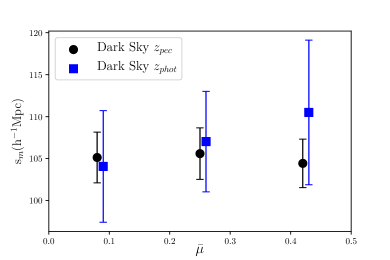
We also verify the internal consistency of the BAO peaks obtained from the Dark Sky photometric catalogue by comparing it with the BAO peaks obtained from the true redshift ($z_{pec}$, cosmological redshift with peculiar velocity added) catalogue for the same $\bar{\mu}$ bins. The wedge correlation functions from the three $\bar{\mu}$ bins are calculated using Eq. 3 and the $s_{m}$ values obtained from the two samples are plotted in Figure 6. For all the three $\bar{\mu}$ bins, it can be seen that the $s_{m}$ values from the photometric samples are within 1$\sigma$ compared to the $s_{m}$ values from the $z_{pec}$ sample, with the $1\sigma$ errors on $s_{m}$ being larger for the $z_{phot}$ sample.

Figure 5: Top panel: $\xi_{w}(s,\mu)\,$(multiplied by $s^{2}$) calculated for the DECaLS data (dotted points in red, same as in Figure 2) compared with $\xi_{w}(s,\mu)\,$calculated for the Dark Sky simulation (solid lines in blue) within the redshift range $0.6<z_{phot}<0.8$ for the three $\mu=0.08,0.25,0.42$ bins from left to right. Bottom panel: Same plot for the samples within the redshift range $0.8<z_{phot}<1.0$. A constant value of 0.0005 and 0.0010 has been added to the $\xi_{w}(s,\mu)\,$from the Dark Sky mocks for the $0.6<z_{phot}<0.8$ and $0.8<z_{phot}<1.0$ samples respectively so that the amplitudes match with the $\xi_{w}(s,\mu)\,$from the DECaLS data. The error bars are the square root of the diagonal elements of the full covariance matrix as mentioned in Eq. 7. The error bars for the Dark Sky sample are represented by the shaded blue region.

Figure 6: The x-axis denotes the 3 $\bar{\mu}$ bins we have used and the y-axis denotes the value of $s_{m}$ obtained from the empirical fit for the Dark Sky $z_{pec}$ sample (black dots) and the Dark Sky $z_{phot}$ sample (blue dots) within the redshift range $0.6<z_{phot}<0.8$. The $\bar{\mu}$ bins for the $z_{phot}$ sample have been shifted by 0.01 for better visualisation.

4 Measured cosmic distances

In the previous section, we measured the BAO peak position $s_{m}$ for our DECaLS sample at different $\bar{\mu}$ bins. In this section, we explain the theoretical model which we use to obtain the theoretical correlation function $\xi_{\rm th}(s,\mu)$. The $\xi_{\rm th}$ is a function of both $s$ and $\mu$, which can then be used to translate our measured BAO peak positions to physical distances.

The volume distance at a redshift is given by,

$$D_{V}(z)=\left[(1+z)^{2}D_{A}(z)^{2}cz/H(z)\right]^{1/3}$$ (12)

and is measured through the BAO by exploiting the monopole correlation function ($\xi_{0}$). It has been shown from previous studies (Estrada et al., 2009; Sridhar & Song, 2019) that for photometric redshift samples, the BAO peak is smeared out in $\xi_{0}$. Thus, using the wedge approach, both the transverse and radial cosmic distances can be separately measured.

4.1 Theoretical model for the correlation function

We compute the theoretical correlation function $\xi_{\rm th}(s,\mu)$ in redshift space exploiting the improved power spectrum based upon the TNS model as,

$$\xi_{\rm th}(s,\mu) = \int\frac{d^{3}k}{(2\pi)^{3}}\tilde{P}(k,\mu^{\prime})e^{i{\bf k}\cdot{\bf s}}$$ (13)

$$= \sum_{\ell:{\rm even}}\xi_{\ell}(s){\cal P}_{\ell}(\mu)\,,$$

with ${\cal P}$ being the Legendre polynomials. Here, we define $\mu=\pi/s$ and $s=(\sigma^{2}+\pi^{2})^{1/2}$. The moments of the correlation function, $\xi_{\ell}(s)$, are defined by,

$$\xi_{\ell}(s)=i^{\ell}\int\frac{k^{2}dk}{2\pi^{2}}\,\tilde{P}_{\ell}(k)\,j_{\ell}(ks)\,.$$ (14)

The multipole power spectra $\tilde{P}_{\ell}(k)$ are explicitly given by,

$$\tilde{P}_{0}(k) = p_{0}(k),$$

$$\tilde{P}_{2}(k) = \frac{5}{2}\left[3p_{1}(k)-p_{0}(k)\right],$$

$$\tilde{P}_{4}(k) = \frac{9}{8}\left[35p_{2}(k)-30p_{1}(k)+3p_{0}(k)\right],$$

where we define the function $p_{m}(k)$:

$$p_{m}(k) = \frac{1}{2}\sum_{n=0}^{4}\frac{\gamma(m+n+1/2,\kappa)}{\kappa^{m+n+1/2}}\,Q_{2n}(k)$$ (16)

with $\kappa=k^{2}\sigma_{p}^{2}$. The function $\gamma$ is the incomplete gamma function of the first kind:

$$\gamma(n,\kappa)=\int^{\kappa}_{0}dt\,t^{n-1}\,e^{-t}\,.$$ (17)

The $Q_{2n}$ is explained below.

The observed power spectrum in redshift space $\tilde{P}(k,\mu)$ is written in the following form;

$$\tilde{P}(k,\mu)=\sum_{n=0}^{8}\,Q_{2n}(k)\mu^{2n}\,G^{\rm FoG}(k\mu\sigma_{p})\,,$$ (18)

where the velocity dispersion $\sigma_{p}$ is set to be a free parameter for FoG effect, and the function $Q_{2n}$ are given by,

$$Q_{0}(k) = P_{\delta\delta}(k),$$

$$Q_{2}(k) = 2P_{\delta\Theta}(k)+C_{2}(k),$$

$$Q_{4}(k) = P_{\Theta\Theta}(k)+C_{4}(k),$$ (19)

where $C_{n}$ includes the higher order polynomials caused by the correlation between density and velocity fluctuations, and $P_{XY}(k)$ denotes the power spectrum in real space. The standard perturbation model exhibits the ill-behaved expansion leading to the bad UV behaviour. In this manuscript, we use the resummed perturbation theory RegPT which is regularised by introducing UV cut-off Taruya et al. (2012). The auto and cross spectra of $P_{XY}(k)$ are computed up to first order, and higher order polynomials are computed up to zeroth order, which are consistent in the perturbative order.

Figure 7: Left panel: The $D_{A}(z)\times(r_{d,fid}/r_{d})$ measurements obtained from the two redshift samples are plotted in red along with the values of $D_{A}(z)\times(r_{d,fid}/r_{d})$ measured by other surveys (as colour coded in the legend and mentioned in the text). The solid black line corresponds to the theoretical predictions for $D_{A}(z)$ as a function of redshift obtained using the cosmological parameters measured from Planck Collaboration et al. (2018). Units are in Mpc. The normalised likelihood $\mathscr{L}$ = exp$(-\Delta\chi^{2}/2)$ for $D_{A}(z)$ obtained for the $0.6<z_{phot}<0.8$ (solid red line) and the $0.8<z_{phot}<1.0$ sample (dotted red line) is plotted in the inset plot. Right panel: The value of $H_{0}$ obtained using the likelihoods from our $D_{A}$ measurements (on top) compared with $H_{0}$ measurements from different probes with $1\sigma$ error bars. The $1\sigma$ error from the Planck Collaboration et al. (2018) (constraints including BAO) is plotted in light green and the $1\sigma$ error from Riess et al. (2019) is plotted in light blue. From bottom to top, enumerated on the vertical axis, Tröster et al. (2020) (BOSS DR12 constraints from anisotropic clustering measurements), Colas et al. (2019) (SDSS/BOSS DR12 constraints using effective field theory), Domínguez et al. (2019) ($\gamma$-ray attenuation), Abbott et al. (2017) (LIGO binary black hole merger GW170817), Fernández Arenas et al. (2018) (HII galaxies), Yu et al. (2018) (cosmic chronometers + BAO), Yuan et al. (2019) (TRGB calibrated SNIa), Wong et al. (2019) (H0LiCOW, gravitationally lensed quasars), Abbott et al. (2018) (DES clustering + weak lensing).

Although cosmic distances are estimated using the BAO at linear regimes, there are smearing effects at small scales which need to be computed. These small scale corrections are included to make the final precise constraints on the BAO (Taruya et al., 2010). We make use of an improved model of the redshift-space power spectrum (Taruya et al., 2010), in which the coupling between the density and velocity fields associated with the Kaiser and the FoG effects is perturbatively incorporated into the power spectrum expression. The resultant includes nonlinear corrections consisting of higher-order polynomials (Taruya et al., 2010):

$$\hat{P}(k,\mu) = \big{\{}P_{\delta\delta}(k)+2\mu^{2}P_{\delta\Theta}(k)+\mu^{4}P_{\Theta\Theta}(k)$$ (20)

$$+ A(k,\mu)+B(k,\mu)\big{\}}G^{\rm FoG}$$

Here the $A(k,\mu)$ and $B(k,\mu)$ terms are the nonlinear corrections, and are expanded as power series of $\mu$. Those spectra are computed using the fiducial cosmological parameters. The FoG effect $G^{\rm FoG}$ is given by the simple Gaussian function which is written as,

$$G^{\rm FoG}\equiv\exp{\left[-(k\mu\sigma_{p})^{2}\right]}$$ (21)

where $\sigma_{p}$ denotes one dimensional velocity dispersion.

Thus the theoretical correlation function $\xi_{\rm th}(s,\mu)$ is parameterised by,

$$x_{\rm th}=(D_{A},H^{-1},G_{b},G_{\Theta},\sigma_{p})$$ (22)

wherein $G_{b}$ and $G_{\Theta}$ are the normalised density and coherent motion growth functions. When working with photo-z samples, the effect of the photo-z error on the correlation function is incoherent. Thus, an extra parameter is needed for the theoretical template to model $\xi_{\rm th}(s,\mu)$ as a function of the photo-z error, but it is not well understood. So, we use Eq. 4 instead to fit our observed $\xi_{w}(s,\mu)\,$. This functional form only assumes a power-law at small scales and a Gaussian function to fit the BAO peak at large scales and seems to model $\xi_{w}(s,\mu)\,$quite well as we can see from Fig. 2.

In our previous work (Sridhar & Song, 2019) we have verified that the BAO feature from the theoretical correlation function is weakly dependent on the growth functions and $\sigma_{p}$. We have verified that changing the value of $\sigma_{p}$ by $\pm$10% does alter the location of the BAO peak, but only by less than 0.1% for samples at $\bar{\mu}$ close to 0 and less than 1% for samples at $\bar{\mu}$ close to 1, which is negligible. Thus, when we fit the cosmic distances, we fix $\sigma_{p}$. To find the best-fit $\sigma_{p}$, we vary it within $3.0<\sigma_{p}(\mathrm{h}^{-1}\mathrm{Mpc})<6.0$ (by fixing $D_{A}$ and $H^{-1}$ to their fiducial values), compute the theoretical correlation function $\xi_{\rm th}(s,\mu)$ and use the $\sigma_{p}$ for which $\xi_{\rm th}(s,\mu)$ matches best with our measured $\xi_{w}(s,\mu)\,$. The best fit $\sigma_{p}$ used in this works is $\sigma_{p}=4.8\,\mathrm{h}^{-1}\mathrm{Mpc}$, and we fix it for both the redshift ranges.

Note that we apply the TNS model for computing the theoretical BAO peaks to fit the measured data. It has been shown in Sridhar & Song (2019) that using a simple coordinate transformation to transform the theoretical BAO peaks from one cosmology to another results in incorrect values of the BAO peak especially at high $D_{A}$ and $H^{-1}$ values. Thus, the TNS model is adopted to determine the theoretical BAO points rather than a simple coordinate transformation.

4.2 Cosmic distance measurements

In Section 3.3, we obtained the $s_{m}$ values for our two redshift samples from the DECaLS data. In this section, we explain how we use a two-step process to go from $s_{m}$ to measured cosmic distances $D_{A}$ and $H^{-1}$. As mentioned in the previous section, $\xi_{\rm th}$ is a function of $s$ and $\mu$ and depends on 5 parameters as mentioned in Eq. 22. Since $\xi_{\rm th}(s,\mu)$ is weakly dependent on the growth functions ($G_{b}$ and $G_{\Theta}$) and $\sigma_{p}$, we vary the tangential and radial distance measures from the fiducial values of $D_{A}$ and $H^{-1}$ for the two redshift samples when we fit the cosmic distances. We use a $13\times 13$ grid for varying $D_{A}$ and $H^{-1}$ and both $D_{A}$ and $H^{-1}$ are sampled within $0.6(param^{fid})<param^{fid}<1.4(param^{fid})$, where $param$ is either $D_{A}$ or $H^{-1}$. For each of these parameter set we obtain a $\xi_{\rm th}(s,\mu)$ for the given $\mu$. We then fit each of our $\xi_{\rm th}(s,\mu)$ function using Eq.4 to obtain the theoretical $s_{m}$ values. We then compare the $\xi_{\rm th}(s,\mu)$ with our measured $\xi_{w}(s,\mu)\,$and compute the $\chi^{2}$ values using the $s_{m}$ values from the DECaLS data and the theoretical templates for the first 3 $\bar{\mu}$ bins (as we find that the BAO peak is washed-out for the last three $\bar{\mu}$ bins) taking into account the covariance between the $s_{m}$ values between the different $\bar{\mu}$ bins that exist.

The uncertainty on the redshift determination prevents us from accessing the radial cosmic distance, and thus the BAO peak is not clearly visible for the $\xi(s,\bar{\mu}>0.5)$ correlation functions. Thus, we do not get tight constraints on $H^{-1}(z)$. However, even after fully marginalising over $H^{-1}(z)$, the transverse cosmic distance $D_{A}(z)\times(r_{d,fid}/r_{d})$ is measured with good precision for both the redshift samples. The fiducial values of $D_{A}^{fid}$ for our cosmology at the two mean redshifts is $D_{A}^{fid}(\bar{z}=0.697)=1514$ Mpc and $D_{A}^{fid}(\bar{z}=0.874)=1638$ Mpc and the measured values are:

$$D_{A}(0.697)=(1499\pm 77\,\mathrm{Mpc})\left(\frac{r_{d}}{r_{d,fid}}\right),$$ (23)

$$D_{A}(0.874)=(1680\pm 109\,\mathrm{Mpc})\left(\frac{r_{d}}{r_{d,fid}}\right),$$ (24)

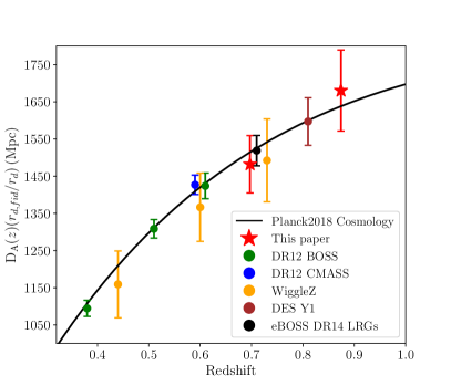
These values correspond to distance measures of 5.14% and 6.48% precision for the two redshift samples respectively. The 0.2% statistical error on $r_{d}$ based on the Planck Collaboration et al. (2018) measurements only make a negligible contribution when added in the above equations. We compare our results with previous studies in Figure 7. The constraints using four spectroscopic redshift surveys, i.e. Blake et al. (2011) (WiggleZ), Alam et al. (2017) (DR12 BOSS), Chuang et al. (2017) (DR12 CMASS) and Bautista et al. (2018) (DR14 eBOSS) are plotted in yellow, green, blue and black respectively. The constraints using the DES photometric redshift survey (The Dark Energy Survey Collaboration et al. (2017)) is plotted in brown. The solid black line corresponds to the theoretical predictions as a function of redshift obtained using the cosmological parameters from Planck Collaboration et al. (2018).

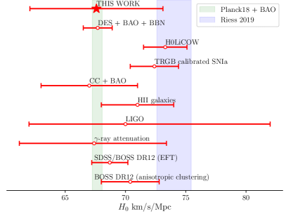
The cosmological concordance model with the cosmological constant is assumed to be a cause of cosmic acceleration, with the Hubble constant unknown. The measured angular diameter distance at the two redshifts from the DECaLS sample and the prior information of the sound horizon size and $w_{m}\equiv\Omega_{m}h^{2}=0.1430\pm 0.0011$ as determined by the Planck experiment (Planck Collaboration et al. (2018)) are used to get constraints on $H_{0}$. The $\chi^{2}$ values from $D_{A}(z)$ along with the $\chi^{2}$ values from $w_{m}$ are cumulatively summed up to get the final constraint on $H_{0}$. We fit for the three parameters ($\Omega_{m},\Omega_{m}h^{2},H_{0}$) using flat, wide priors which extend well beyond the regions of high likelihood and have no effect on the cosmological fits and obtain a value of $H_{0}=67.59\pm 5.52$ km/s/Mpc.

We also make a comparison plot with $H_{0}$ measurements obtained from recent works using different probes in the right panel of Figure 7. Our $H_{0}$ value is measured with 8.1% precision, whereas some of the estimates from other probes plotted in Figure 7 have a better precision. To quote a few, the HII galaxy data (Fernández Arenas et al., 2018) delivers a $\sigma_{H_{0}}/H_{0}$ = 4.9%, the DES + BAO + BBN data delivers a $\sigma_{H_{0}}/H_{0}$ = 1.8%. The reason for our conservative estimate is because we only use the likelihoods from our $D_{A}(z)$ measurements which have been obtained from photometric redshift samples. We have used the prior information of the sound horizon scale and $w_{m}$ from Planck like other BAO studies. We believe that the photo-z error is subdominant compared to the error that we get from cosmic variance. The DESI catalogue and the DECaLS catalogue share the same footprint and so the cosmic variance will be minimal, however, due to the photo-z uncertainty, the error on the $H_{0}$ value we obtain increases. It can be seen that our mean value of $H_{0}=67.59$ km/s/Mpc is well within $1\sigma$ of the Planck18 + BAO value.

5 Discussion and conclusions

We provide a statistical methodology to extract cosmic distance information using BAO peaks only from the DECaLS DR8 LRG photometric galaxy sample. Common practice to extract the BAO peak from photometric redshift catalogues is by measuring the incomplete angular correlation function. In this manuscript, we make use of the wedge correlation function, wherein we split the sample into small wedges and include the BAO information from all the wedges in which they are still present ($\bar{\mu}<0.5$, above which there is noticeable contamination). Transverse cosmic distance $D_{A}(z)$ is measured with good precision for both the redshift samples giving us values of $D_{A}(\bar{z}=0.69)=1499\pm 77\,\mathrm{Mpc}(r_{d}/r_{d,fid})$ and $D_{A}(\bar{z}=0.87)=1680\pm 109\,\mathrm{Mpc}(r_{d}/r_{d,fid})$ with a fractional error of 5.14% and 6.48% respectively. The values that we obtain have been compared with the theoretical prediction for $D_{A}(z)$ as a function of redshift obtained using the cosmological parameters measured from Planck Collaboration et al. (2018) and are well within the $1\sigma$ region.

We have also compared our results with the results of $D_{A}(z)$ obtained from other similar surveys (both spectroscopic and photometric) and find them to be consistent with each other. Since most radial information is contained at the $\bar{\mu}>0.5$ bins which are contaminated by the photometric redshift uncertainty, we are not able to extract information on the radial cosmic distance. This is the first time that $D_{A}(z)$ is constrained at such a high redshift ($\bar{z}=0.87$) using LRGs.

Most of the recent works (Sánchez et al., 2011; Carnero et al., 2012; Seo et al., 2012) have used the angular correlation function $w(\theta)$ to get cosmic distance measures using several narrow redshift slices. Since radial binning blends data beyond what is induced by the photometric redshift error, the full information that is present is not utilised. Another important aspect that is often ignored when calculating $w(\theta)$ is the cross correlation between the different redshift bins used along with the complications that it brings with calculating the covariance matrix, i.e. the computing time increases with the number of bins in $\theta$ and number of redshift slices used.

The full spectroscopy DESI galaxy catalogue will be available around 2025 and will cover the footprint observed by DECaLS, but with higher precision. Here we try to probe the cosmological signature imprinted in this photometric footprint map. Most BAO measurements (Anderson et al., 2012; Alam et al., 2017; Chuang et al., 2017) at low redshifts have supported the $H_{0}$ measurement by the Planck experiment, and it becomes interesting to see whether DESI will provide a similar result or not. By using the information obtained on the angular diameter distance from the DECaLS samples at the two median redshifts along with prior information of the sound horizon from Planck, we try to provide a precursor for the $H_{0}$ value expected from DESI. Although precise information of $H_{0}$ is not possible from photometric redshift catalogues, we obtain a value of $H_{0}=67.59\pm 5.52$ km/s/Mpc with a fractional error of 8.16%. Our value of $H_{0}$ supports the $H_{0}$ measured by all other BAO results and is consistent with the $\Lambda$CDM model.

Appendix A Systematic contamination from stellar density

Systematic effects are often present in an imaging dataset such as the DECaLS dataset, which can lead to spurious fluctuations in the target density and in turn to changes in the shape of the redshift distribution. One such major contribution towards systematic contamination in the data comes from correlations with stellar density (Rezaie et al., 2019). To check for this systematic effect, we compare our DECaLS LRG density and the density of the random catalogue with the density of Gaia stars. First, we convert the sky coordinates (RA and DEC) from our data and random catalogue into HEALPIX pixels using the same $nside=256$ as used for the Gaia stellar density maps. We then use the Pearson correlation coefficient (PCC) to assess the linear correlation between the two datasets. For two variables $X$ and $Y$, the PCC is defined as,

$$\rho_{X,Y}=\frac{cov(X,Y)}{\sqrt{cov(X,X)cov(Y,Y)}}$$ (A1)

where $cov(X,Y)$ is the covariance between $X$ and $Y$ across all pixels. We get a value of $\rho_{X,Y}=-0.0416$ for $X$ and $Y$ being the Gaia stellar density and DECaLS LRG density and $\rho_{X,Y}=-0.0443$ for $X$ and $Y$ being the Gaia stellar density and random catalogue density, which shows that there is almost no strong positive or negative correlation between the two datasets separately.

(a)

(b)

(c)

(d)

(e)

(f)

Figure 8: First row: Comparison of the correlation function $\xi_{w}(s,\mu)\,$(multiplied by $s^{2}$ ) for $\bar{\mu}=0.08,0.25,0.42$ (from the $0.6<z_{phot}<0.8$ sample) between the DECaLS data (given by red dots) and the mean $\xi_{w}(s,\mu)\,$of the 100 EZmock samples (given by the solid blue line) generated by the Gaussian approximation method. The photo-z’s for all the EZmock samples have been created by extracting a random $\sigma_{z}$ from the parent DECaLS sample. The $\xi_{w}(s,\mu)\,$from all the 100 samples are plotted as lighter blue lines in the background. Note: We have added a constant value of 0.0020 to the EZmock $\xi_{w}(s,\mu)\,$for the $0.6<z_{phot}<0.8$ sample for the amplitudes to match. Second row: The same as above, but for the $0.8<z_{phot}<1.0$ sample. We have added a constant value of 0.0015 to the EZmock $\xi_{w}(s,\mu)\,$for the $0.8<z_{phot}<1.0$ sample for the amplitudes to match.

Appendix B Comparison of the clustering results between DECaLS and EZmock

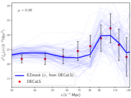
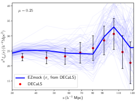
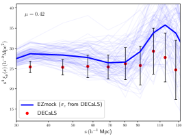
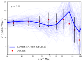
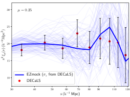
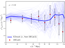
As mentioned in Section 2.3, we generate photo-z’s for the EZmock samples from random $\sigma_{z}$ values obtained from the DECaLS data by restricting to galaxies of similar redshifts. We calculate $\xi_{w}(s,\mu)\,$for the 100 EZmock samples separately using the same $s$ and $\mu$ binning scheme as mentioned in Section 3.3 and the mean $\xi_{w}(s,\mu)\,$for both the redshift samples is plotted as the solid blue line in Figure 8. We find that by using the true values of $\xi_{w}(s,\mu)\,$for the two redshift samples from the EZmock, the amplitudes of $\xi_{w}(s,\mu)\,$do not match. However, by adding adding a constant value (0.0020 for the $0.6<z_{phot}<0.8$ sample and 0.0015 for the $0.8<z_{phot}<1.0$ sample) to the $\xi_{w}(s,\mu)\,$, we see that the mean $\xi_{w}(s,\mu)\,$of the obtained from the EZmock photo-z’s created by randomly selecting $\sigma_{z}$’s from the DECaLS sample match closely to the DECaLS $\xi_{w}(s,\mu)\,$, especially at the BAO scales as shown in Figure 8. To statistically measure the significance of the similarity, we use the KS test on both the redshift samples. The null hypotheses for the KS test is that the distributions are the same and to reject the null hypotheses we require a $p$-value (significance) less than 0.05. For the $0.6<z_{phot}<0.8$ sample, we obtain a $p$-value of 0.78 and 0.18 for the $\bar{\mu}=0.08$ and 0.25 samples respectively. For the $\bar{\mu}=0.42$ sample, we however obtain a $p$-value of 0.004 which rules out the null hypotheses. We however, believe that this should not have a significant impact on the covariance matrix obtained and should be conservative. For the $0.8<z_{phot}<1.0$ sample, the minimum $p$-value we obtain from all the three $\bar{\mu}$ bins is 0.48, which does not rule out the null hypotheses. When adding the constant, we assume that there is some bias in the data, but we do not expect that it would change the covariance matrix.

As a further test, we fit the mean $\xi_{w}(s,\mu)\,$from the 100 EZmock samples for the two redshift bins using the MCMC technique with the same fitting parameter space as given by Eq.5. We apply the same priors to all our samples as mentioned in Section 3.1. The values of $s_{m}$ obtained from the MCMC fit for the two samples are given in Table 3. First we compare the $s_{m}$ value obtained from the EZmock samples with the same obtained from the DECaLS data. It can be seen that the common trend of $s_{m}$ increasing with $\bar{\mu}$ bin is also observed for the EZmock sample in both the redshift ranges considered. The errors obtained on $s_{m}$ for the EZmock samples are similar to what we have obtained for the DECaLS sample in both the redshift ranges, with the error on $s_{m}$ increasing with $\bar{\mu}$.

The obtained $s_{m}$ values from the EZmock samples are converted to physical distances using the same methodology as explained in Section 4.2. For the $0.6<z_{phot}<0.8$ and $0.8<z_{phot}<1.0$ samples we obtain values of $D_{A}(0.69)=1507\pm 58\,\mathrm{Mpc}(r_{d}/r_{d,fid})$ and $D_{A}(0.87)=1616\pm 84\,\mathrm{Mpc}(r_{d}/r_{d,fid})$. These values correspond to distance measures of 3.88% and 5.2% precision for the two redshift samples respectively. It can also be noted that the recovered values of $D_{A}$ for the EZmock samples are a good match to the expected values $D_{A}^{fid}$ from the fiducial cosmology we use. The fiducial values of $D_{A}^{fid}$ for our cosmology at the two mean redshifts is $D_{A}^{fid}(\bar{z}=0.697)=1514$ Mpc (0.4% higher than the recovered value) and $D_{A}^{fid}(\bar{z}=0.874)=1638$ Mpc (1.3% higher than the recovered value). Given the overall precision, these values are well within the expected limits.

Redshift range	$\bar{\mu}$ bin	$s_{m}$ (h-1Mpc)
	0.08	$106.7^{+3.1}_{-3.5}$
$0.6<z_{phot}<0.8$	0.25	$111.4^{+3.9}_{-4.2}$
	0.42	$114.4^{+5.9}_{-4.7}$
	0.08	$107.6^{+5.0}_{-4.8}$
$0.8<z_{phot}<1.0$	0.25	$107.9^{+5.1}_{-4.3}$
	0.42	$112.3^{+6.0}_{-5.1}$

Table 3: Results of fitting the EZmock correlation function for the two redshift samples and in the 3 $\bar{\mu}$ bins using Eq. 4. The $s_{m}$ is the BAO peak point obtained from the fit and the units are in h^-1Mpc.

References

- Abbott et al. (2017) Abbott, B. P., Abbott, R., Abbott, T. D., et al. 2017, Nature, 551, 85, doi: 10.1038/nature24471
- Abbott et al. (2018) Abbott, T. M. C., Abdalla, F. B., Annis, J., et al. 2018, MNRAS, 480, 3879, doi: 10.1093/mnras/sty1939
- Alam et al. (2017) Alam, S., Ata, M., Bailey, S., et al. 2017, MNRAS, 470, 2617, doi: 10.1093/mnras/stx721
- Anderson et al. (2012) Anderson, L., Aubourg, E., Bailey, S., et al. 2012, MNRAS, 427, 3435, doi: 10.1111/j.1365-2966.2012.22066.x
- Arnalte-Mur et al. (2009) Arnalte-Mur, P., Fernández-Soto, A., Martínez, V. J., et al. 2009, MNRAS, 394, 1631, doi: 10.1111/j.1365-2966.2009.14430.x
- Astropy Collaboration et al. (2013) Astropy Collaboration, Robitaille, T. P., Tollerud, E. J., et al. 2013, aap, 558, A33, doi: 10.1051/0004-6361/201322068
- Aubourg et al. (2015) Aubourg, E., Bailey, S., Bautista, J. E., et al. 2015, Phys. Rev. D, 92, 123516, doi: 10.1103/PhysRevD.92.123516
- Bautista et al. (2018) Bautista, J. E., Vargas-Magaña, M., Dawson, K. S., et al. 2018, ApJ, 863, 110, doi: 10.3847/1538-4357/aacea5
- Behroozi et al. (2013) Behroozi, P. S., Wechsler, R. H., & Wu, H.-Y. 2013, ApJ, 762, 109, doi: 10.1088/0004-637X/762/2/109
- Benedict et al. (1999) Benedict, G. F., McArthur, B., Chappell, D. W., et al. 1999, AJ, 118, 1086, doi: 10.1086/300975
- Blake et al. (2011) Blake, C., Davis, T., Poole, G. B., et al. 2011, MNRAS, 415, 2892, doi: 10.1111/j.1365-2966.2011.19077.x
- Breiman (2001) Breiman, L. 2001, Machine Learning, 45, 5, doi: 10.1023/A:1010933404324
- Carnero et al. (2012) Carnero, A., Sánchez, E., Crocce, M., Cabré, A., & Gaztañaga, E. 2012, MNRAS, 419, 1689, doi: 10.1111/j.1365-2966.2011.19832.x
- Chuang et al. (2015) Chuang, C.-H., Kitaura, F.-S., Prada, F., Zhao, C., & Yepes, G. 2015, MNRAS, 446, 2621, doi: 10.1093/mnras/stu2301
- Chuang et al. (2017) Chuang, C.-H., Pellejero-Ibanez, M., Rodríguez-Torres, S., et al. 2017, MNRAS, 471, 2370, doi: 10.1093/mnras/stx1641
- Colas et al. (2019) Colas, T., D’Amico, G., Senatore, L., Zhang, P., & Beutler, F. 2019, Efficient Cosmological Analysis of the SDSS/BOSS data from the Effective Field Theory of Large-Scale Structure. https://arxiv.org/abs/1909.07951
- Davis & Peebles (1983) Davis, M., & Peebles, P. J. E. 1983, ApJ, 267, 465, doi: 10.1086/160884
- DESI Collaboration et al. (2016) DESI Collaboration, Aghamousa, A., Aguilar, J., et al. 2016, arXiv e-prints, arXiv:1611.00036. https://arxiv.org/abs/1611.00036
- Dey et al. (2018) Dey, A., Schlegel, D. J., Lang, D., et al. 2018, ArXiv e-prints. https://arxiv.org/abs/1804.08657
- Domínguez et al. (2019) Domínguez, A., Wojtak, R., Finke, J., et al. 2019, ApJ, 885, 137, doi: 10.3847/1538-4357/ab4a0e
- Eisenstein et al. (1998) Eisenstein, D. J., Hu, W., & Tegmark, M. 1998, ApJ, 504, L57, doi: 10.1086/311582
- Eisenstein et al. (2005) Eisenstein, D. J., Zehavi, I., Hogg, D. W., et al. 2005, ApJ, 633, 560, doi: 10.1086/466512
- Estrada et al. (2009) Estrada, J., Sefusatti, E., & Frieman, J. A. 2009, ApJ, 692, 265, doi: 10.1088/0004-637X/692/1/265
- Euclid Collaboration et al. (2019) Euclid Collaboration, Adam, R., Vannier, M., et al. 2019, A&A, 627, A23, doi: 10.1051/0004-6361/201935088
- Farrow et al. (2015) Farrow, D. J., Cole, S., Norberg, P., et al. 2015, MNRAS, 454, 2120, doi: 10.1093/mnras/stv2075
- Fernández Arenas et al. (2018) Fernández Arenas, D., Terlevich, E., Terlevich, R., et al. 2018, MNRAS, 474, 1250, doi: 10.1093/mnras/stx2710
- Fernie (1969) Fernie, J. D. 1969, PASP, 81, 707, doi: 10.1086/128847
- Foreman-Mackey et al. (2013) Foreman-Mackey, D., Hogg, D. W., Lang, D., & Goodman, J. 2013, PASP, 125, 306, doi: 10.1086/670067
- Hartlap et al. (2007) Hartlap, J., Simon, P., & Schneider, P. 2007, A&A, 464, 399, doi: 10.1051/0004-6361:20066170
- Hong et al. (2012) Hong, T., Han, J. L., Wen, Z. L., Sun, L., & Zhan, H. 2012, ApJ, 749, 81, doi: 10.1088/0004-637X/749/1/81
- Howlett et al. (2012) Howlett, C., Lewis, A., Hall, A., & Challinor, A. 2012, JCAP, 1204, 027, doi: 10.1088/1475-7516/2012/04/027
- Kazin et al. (2013) Kazin, E. A., Sánchez, A. G., Cuesta, A. J., et al. 2013, MNRAS, 435, 64, doi: 10.1093/mnras/stt1261
- Lewis et al. (2000) Lewis, A., Challinor, A., & Lasenby, A. 2000, Astrophys. J., 538, 473, doi: 10.1086/309179
- Meisner et al. (2017) Meisner, A. M., Lang, D., & Schlegel, D. J. 2017, AJ, 153, 38, doi: 10.3847/1538-3881/153/1/38
- Navarro et al. (1996) Navarro, J. F., Frenk, C. S., & White, S. D. M. 1996, ApJ, 462, 563, doi: 10.1086/177173
- Padmanabhan et al. (2012) Padmanabhan, N., Xu, X., Eisenstein, D. J., et al. 2012, MNRAS, 427, 2132, doi: 10.1111/j.1365-2966.2012.21888.x
- Peebles & Yu (1970) Peebles, P. J. E., & Yu, J. T. 1970, ApJ, 162, 815, doi: 10.1086/150713
- Percival et al. (2014) Percival, W. J., Ross, A. J., Sánchez, A. G., et al. 2014, MNRAS, 439, 2531, doi: 10.1093/mnras/stu112
- Perlmutter et al. (1999) Perlmutter, S., Aldering, G., Goldhaber, G., et al. 1999, ApJ, 517, 565, doi: 10.1086/307221
- Planck Collaboration et al. (2018) Planck Collaboration, Aghanim, N., Akrami, Y., et al. 2018, arXiv e-prints, arXiv:1807.06209. https://arxiv.org/abs/1807.06209
- Price-Whelan et al. (2018) Price-Whelan, A. M., Sip’ocz, B. M., G”unther, H. M., et al. 2018, aj, 156, 123, doi: 10.3847/1538-3881/aabc4f
- Rezaie et al. (2019) Rezaie, M., Seo, H.-J., Ross, A. J., & Bunescu, R. C. 2019, arXiv e-prints, arXiv:1907.11355. https://arxiv.org/abs/1907.11355
- Riess et al. (2019) Riess, A. G., Casertano, S., Yuan, W., Macri, L. M., & Scolnic, D. 2019, ApJ, 876, 85, doi: 10.3847/1538-4357/ab1422
- Riess et al. (1998) Riess, A. G., Filippenko, A. V., Challis, P., et al. 1998, AJ, 116, 1009, doi: 10.1086/300499
- Ross et al. (2012) Ross, A. J., Percival, W. J., Sánchez, A. G., et al. 2012, MNRAS, 424, 564, doi: 10.1111/j.1365-2966.2012.21235.x
- Ross et al. (2017) Ross, A. J., Banik, N., Avila, S., et al. 2017, MNRAS, 472, 4456, doi: 10.1093/mnras/stx2120
- Sabiu (2018) Sabiu, C. 2018, KSTAT: KD-tree Statistics Package, Astrophysics Source Code Library. http://ascl.net/1804.026
- Sabiu & Song (2016) Sabiu, C. G., & Song, Y.-S. 2016, ArXiv e-prints. https://arxiv.org/abs/1603.02389
- Sánchez et al. (2012) Sánchez, A. G., Scóccola, C. G., Ross, A. J., et al. 2012, MNRAS, 425, 415, doi: 10.1111/j.1365-2966.2012.21502.x
- Sánchez et al. (2013) Sánchez, A. G., Kazin, E. A., Beutler, F., et al. 2013, MNRAS, 433, 1202, doi: 10.1093/mnras/stt799
- Sánchez et al. (2014) Sánchez, A. G., Montesano, F., Kazin, E. A., et al. 2014, MNRAS, 440, 2692, doi: 10.1093/mnras/stu342
- Sánchez et al. (2017) Sánchez, A. G., Scoccimarro, R., Crocce, M., et al. 2017, MNRAS, 464, 1640, doi: 10.1093/mnras/stw2443
- Sánchez et al. (2011) Sánchez, E., Carnero, A., García-Bellido, J., et al. 2011, MNRAS, 411, 277, doi: 10.1111/j.1365-2966.2010.17679.x
- Scolnic et al. (2019) Scolnic, D., Perlmutter, S., Aldering, G., et al. 2019, Astro2020: Decadal Survey on Astronomy and Astrophysics, 2020, 270. https://arxiv.org/abs/1903.05128
- Seo et al. (2012) Seo, H.-J., Ho, S., White, M., et al. 2012, ApJ, 761, 13, doi: 10.1088/0004-637X/761/1/13
- Skillman et al. (2014) Skillman, S. W., Warren, M. S., Turk, M. J., et al. 2014, arXiv e-prints, arXiv:1407.2600. https://arxiv.org/abs/1407.2600
- Sridhar et al. (2017) Sridhar, S., Maurogordato, S., Benoist, C., Cappi, A., & Marulli, F. 2017, A&A, 600, A32, doi: 10.1051/0004-6361/201629369
- Sridhar & Song (2019) Sridhar, S., & Song, Y.-S. 2019, MNRAS, 488, 295, doi: 10.1093/mnras/stz1716
- Taruya et al. (2012) Taruya, A., Bernardeau, F., Nishimichi, T., & Codis, S. 2012, Phys. Rev. D, 86, 103528, doi: 10.1103/PhysRevD.86.103528
- Taruya et al. (2010) Taruya, A., Nishimichi, T., & Saito, S. 2010, Phys. Rev. D, 82, 063522, doi: 10.1103/PhysRevD.82.063522
- Taylor (2005) Taylor, M. B. 2005, in Astronomical Society of the Pacific Conference Series, Vol. 347, Astronomical Data Analysis Software and Systems XIV, ed. P. Shopbell, M. Britton, & R. Ebert, 29
- The Dark Energy Survey Collaboration (2005) The Dark Energy Survey Collaboration. 2005, ArXiv Astrophysics e-prints
- The Dark Energy Survey Collaboration et al. (2017) The Dark Energy Survey Collaboration, Abbott, T. M. C., Abdalla, F. B., et al. 2017, arXiv e-prints, arXiv:1712.06209. https://arxiv.org/abs/1712.06209
- The Planck Collaboration (2006) The Planck Collaboration. 2006, arXiv e-prints, astro. https://arxiv.org/abs/astro-ph/0604069
- Totsuji & Kihara (1969) Totsuji, H., & Kihara, T. 1969, PASJ, 21, 221
- Tröster et al. (2020) Tröster, T., Sánchez, A. G., Asgari, M., et al. 2020, Astronomy and Astrophysics, 633, L10, doi: 10.1051/0004-6361/201936772
- Veropalumbo et al. (2014) Veropalumbo, A., Marulli, F., Moscardini, L., Moresco, M., & Cimatti, A. 2014, MNRAS, 442, 3275, doi: 10.1093/mnras/stu1050
- Veropalumbo et al. (2016) —. 2016, MNRAS, 458, 1909, doi: 10.1093/mnras/stw306
- Wong et al. (2019) Wong, K. C., Suyu, S. H., Chen, G. C. F., et al. 2019, arXiv e-prints, arXiv:1907.04869. https://arxiv.org/abs/1907.04869
- Wright et al. (2010) Wright, E. L., Eisenhardt, P. R. M., Mainzer, A. K., et al. 2010, AJ, 140, 1868, doi: 10.1088/0004-6256/140/6/1868
- Yu et al. (2018) Yu, H., Ratra, B., & Wang, F.-Y. 2018, ApJ, 856, 3, doi: 10.3847/1538-4357/aab0a2
- Yuan et al. (2019) Yuan, W., Riess, A. G., Macri, L. M., Casertano, S., & Scolnic, D. M. 2019, ApJ, 886, 61, doi: 10.3847/1538-4357/ab4bc9
- Zhou et al. (2020) Zhou, R., Newman, J. A., Mao, Y.-Y., et al. 2020, arXiv e-prints, arXiv:2001.06018. https://arxiv.org/abs/2001.06018