State Estimation-Based Robust Optimal Control of Influenza Epidemics in an Interactive Human Society
Abstract
This paper presents a state estimation-based robust optimal control strategy for influenza epidemics in an interactive human society in the presence of modeling uncertainties. Interactive society is influenced by random entrance of individuals from other human societies whose effects can be modeled as a non-Gaussian noise. Since only the number of exposed and infected humans can be measured, states of the influenza epidemics are first estimated by an extended maximum correntropy Kalman filter (EMCKF) to provide a robust state estimation in the presence of the non-Gaussian noise. An online quadratic program (QP) optimization is then synthesized subject to a robust control Lyapunov function (RCLF) to minimize susceptible and infected humans, while minimizing and bounding the rates of vaccination and antiviral treatment. The joint QP-RCLF-EMCKF meets multiple design specifications such as state estimation, tracking, pointwise control optimality, and robustness to parameter uncertainty and state estimation errors that have not been achieved simultaneously in previous studies. The uniform ultimate boundedness (UUB)/convergence of error trajectories is guaranteed using a Lyapunov stability argument. Simulation results show that the proposed approach achieves appropriate tracking and state estimation performance with good robustness on the influenza epidemics of an interactive human society with population of 16000.
keywords:
Influenza epidemics, Interactive human society, State estimation, Robust optimal control1 Introduction
Influenza viruses can cause epidemic human diseases that are currently a worldwide health concern. Proper control of influenza epidemics is a crucial task that can mitigate economic and epidemiological burdens. Recent years have witnessed numerous studies in analysis, modeling, and control of influenza epidemiological systems [3, 36, 25, 28, 17, 11]. Mathematical model of influenza epidemics can provide an opportunity to design model-based control strategies and to analyze the stability of closed-loop systems. Several mathematical models have been proposed for influenza epidemic systems [3, 26, 36]. In [3], compartmental models of the influenza were proposed while considering the vaccination and antiviral treatment as control inputs. In [26], influenza dynamics were modeled by a set of nonlinear differential equations. In [36], a nonlinear SEIAR model of the influenza with two control inputs and five states was described. In this model, the positive state variables S, E, I, A, and R are the Susceptible, Exposed, Infected, Asymptomatic, and Recovered individuals while rates of vaccination and antiviral treatment are considered positive control inputs.
To recover all individuals of a society, the best intervention strategy is desired to be designed for the influenza epidemics. Optimal control is one of the widely-used approach that has been employed to determine the treatment strategies [25, 28, 21, 40, 14]. In [25], an optimal control problem was employed to minimize the number of infected individuals at minimal efforts of the vaccination. Different optimal control strategies were suggested in [28] to minimize the impact of influenza pandemics involving antiviral treatment and/or the isolation measures. In [21], prevention of the pandemic influenza was enhanced towards evaluating time-dependent optimal prevention policies and considering its execution cost. In [40], a dynamic model of an influenza pandemic model was formulated with the existence of vaccination and treatment, and then analyzed in terms of the vaccine intake variations. In [14], a prioritization scheme for allocation of a sizeable quantity of influenza vaccine and antiviral drug was described for a stratified population.
| Abbreviations | |
| MMSE | Minimum mean square error |
| EKF | Extended Kalman filter |
| UKF | Unscented Kalman filter |
| SEIAR | Susceptible, exposed, infected, asymptomatic, and recovered |
| PWMC | Pointwise min-norm control |
| EMCKF | Extended maximum correntropy Kalman filter |
| QP | Quadratic programming |
| ES-CLF | Exponentially stabilizing control Lyanpunov function |
| RCLF | Robust control Lyapunov function |
| UUB | Uniform ultimate boundedness |
Note that the above-mentioned optimal control strategies were formulated with the assumption of fully-known dynamic terms and parameters. However, mathematical models of the influenza epidemics may contain modeling uncertainties that should be taken into account in the control design structure. In [34], a least squares method was employed to estimate unknown parameters of two influenza epidemic models. Although the estimation performance was validated, no any control strategy was designed to minimize the infected population. In [36], a robust adaptive sliding mode controller was designed for a nonlinear SEIAR model of the influenza in the presence of parametric uncertainties. In that work, convergence of susceptible and infected humans to zero was provided by tracking some descending scenarios. Two robust terms were also incorporated in their devised controller whose gains were updated using adaptation laws to compensate for the parameter uncertainties. Stability of closed-loop influenza epidemic system was then proved using a Lyapunov framework and the Barbalat’s lemma.
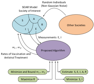
However, that recent paper [36] suffers from several drawbacks. (i) The main one is that the controller requires accurate measurement of state variables, while only the population of exposed and infected humans can be measured in practice. (ii) In that approach, studied human society was assumed to be isolated from other societies. However, a random entrance of individuals from other societies into the main society of interest results in degrading the control performance. This kind of society is called ”interactive society” and the effects from the other societies can be modelled as a non-Gaussian noise as shown in Fig. 1. (iii) In their method, although the convergence of system solutions was obtained and the robustness of closed-loop systems against parametric uncertainties was demonstrated, control optimality, as an important design specification, has not been taken into account. In other words, tracking, robustness, and minimizing the rates of vaccination and antiviral treatment should be achieved at the same time by devising an appropriate control strategy. (iv) In the normalized SEIAR model, the control signals should be always positive and less than 1. However, the approach in [36] was not able to bound the rates of vaccination and antiviral treatment in the controller implementation while facing with high parameter uncertainties and disturbances. It should also be noted that the rest of the above-mentioned papers suffer from the shortcomings mentioned in Items (i) and (iv).
The Kalman filter [22] is still the most common method for state estimation of linear systems because of its optimality and simplicity. However since the mathematical model of the influenza comprises a set of nonlinear differential equations, the extension of Kalman filters, namely the extended Kalman filter (EKF), the unscented Kalman filter (UKF), and particle filters [33, 35, 41, 38, 15, 5, 6, 20, 39], can be alternatively used for the state estimation purpose. A Kalman filter is derived based on the minimum mean square error (MMSE) criterion, which follows that it uses only second-order information of the signal and it is optimal until the gaussianity of noises is preserved. However, in this paper, the performance of the ordinary EKF may break down for the influenza epidemics of an interactive society that is disturbed by non-Gaussian noise (when the society is not isolated). To solve this issue, the maximum correntropy Kalman filter (MCKF) can be utilized to provide robustness for the Kalman filter in the presence of non-Gaussian noise or large outliers [9, 19, 30]. The MCKF uses the correntropy criterion instead of MMSE through which higher-order information of process and measurement noises is used [29, 16].
Motivated by the aforementioned shortcomings of the existing controllers, that have been already designed for the influenza epidemic systems, and the desire to develop a new multi-objective controller for such systems, this work is the first step towards designing a state estimation-based robust optimal controller for influenza epidemics in an interactive human society (demonstrated in Fig. 1) in the presence of modeling uncertainties and non-Gaussian noise. The main contributions of this paper are as follows: (i) the state estimation of the influenza epidemics in an interactive human society; (ii) the design of a robust optimal controller to minimize the population of susceptible and infected humans, while minimizing and bounding the rates of vaccination and antiviral treatment; (iii) the proof of the UUB/convergence of tracking errors; and (iv) the robustness of the proposed algorithm in the presence of parameter perturbation and random entrance of individuals from the other societies.
In this paper, we begin by formulating an extended MCKF (EMCKF) algorithm to estimate the states of an influenza dynamical system while using the number of exposed and infected humans as measurement. With the aim of achieving the boundedness/convergence of system’s errors with a minimal control effort, an online quadratic program (QP) is synthesized subject to a robust control Lyapunov function (RCLF). The joint QP-RCLF finds the optimal balance between control effort and stability of closed-loop system. The robust term is incorporated in the QP-RCLF framework to compensate for state estimation error and modeling uncertainties. The unified state estimation-based controller QP-RCLF-EMCKF provides the convergence of susceptible and infected populations to a small neighborhood around the origin, while minimizing and bounding the control effort. The UUB/convergence of tracking errors is finally proven using a Lyapunov stability argument. To assess the performance of the proposed approach QP-RCLF-EMCKF, simulation results are carried out for the influenza epidemic model. Results show that the proposed controller successfully achieves the promised design specifications such as tracking and state estimation for this epidemiological system. Tests show that the QP-RCLF-EMCKF strategy provides appropriate robustness in the presence of parametric uncertainties and random entrance of humans from other societies to the society of interest.
The paper is organized as follows. Section 2 describes an influenza epidemic model and the problem statement. Section 3 presents the state estimation framework using EMCKF algorithm. Section 4 presents our proposed control strategy QP-RCLF-EMCKF. Section 5 provides the simulation results. Section 6 presents discussion, conclusion, and future work.
2 Influenza Epidemic Model and Problem Statement
In this section, we begin by describing a dynamical model for the influenza epidemics and then present the problem statement.
2.1 Influenza epidemic model
A state space representation of the influenza epidemics can be described by the following nonlinear SEIAR model [36]:
| (1) |
where denotes the state variables of the system with positive values; represents the population that is susceptible to get infected with influenza; is the number of people who are infected with influenza but not yet infectious (exposed); stands for population that is infected and also infectious with influenza symptoms; represents the number of individuals who are influenza carriers but without any symptoms (asymptomatic); denotes the number of recovered humans; is the vector of normalized control inputs such that for ; is the rate of vaccination of the susceptible population ; and is the rate of antiviral treatment of the infected population . More details about this epidemiological model can be found in [4, 27, 36].
2.2 Problem statement
This paper aims to design a robust optimal controller to decrease the number of susceptible and infected populations while using the minimum possible rates of vaccination and antiviral treatment . More importantly, the normalized control inputs must be bounded between 0 and 1, which requires a set of control constraints to be incorporated in the controller design. For this purpose, an online QP control strategy is formulated by considering the RCLF and the above-mentioned input constraints to generate a pointwise optimal control effort, while achieving the convergence of system’s errors.
Since only and are measurable in practice, the proposed controller uses the estimate of system’s states (populations) as feedback in closed-loop system. To achieve a robust state estimation of the influenza epidemics in an interactive human society in the presence of non-Gaussian noise, an EMCKF algorithm is employed and specifically developed for this dynamical system. A robust term is also designed to robutify the system against state estimation error and parametric uncertainties. The resulting state estimation-based control strategy QP-RCLF-EMCKF meets multiple design objectives such as tracking, control optimality, state estimation, and robustness. The UUB/convergence of all system solutions is proven using a Lyapunov framework and the proposed controller is finally validated by comprehensive simulation studies.
3 State Estimation Using Extended Maximum Correntropy Kalman Filter (EMCKF)
In this section, an EMCKF algorithm is described and presented to estimate the system states. This filter only uses the number of exposed and infected humans ( and ) as possible measurements. Consider the following general form of a nonlinear stochastic continuous-time system for the influenza epidemic model (2.1)
| (2) |
where is the vector of measurable variables (populations) in the influenza epidemics; is the continuous-time process noise vector of the system with covariance matrix ; is the continuous-time measurement noise with covariance ; and is the vector of actual system parameters as
| (3) |
Assumption 1
The noises and are both uncorrelated, Gaussian, and zero-mean. However, a shot noise is enforced to the measurement noise to model the effects from the other societies on the main interactive society, which results in a non-Gaussian noise as
| (4) |
Assumption 2
The nonlinear functions and are sufficiently smooth in , such that they can be linearized using the Taylor series expansions.
The EMCKF is similar to the EKF as they are based on linearization using first-order Taylor series expansion. Therefore, the following Jacobian matrices are used to linearize the system:
| (5) |
where and are the estimations of and , respectively. The initialization of the filter is given as:
| (6) |
where stands for the expected value operation; is the covariance of the initial estimate; and and show the initial value of the states and its estimates, respectively.
The state estimate and the EMCKF gain for the continuous-time nonlinear system (2.1) are formulated as follows [37, 12]:
| (7) |
in which the time-varying gain and the estimation error covariance matrix are defined as
| (8) |
with the kernel function defined as
| (9) |
where stands for the Euclidean norm of a vector; denotes a weighted Euclidean norm of a vector (i.e., with 111It should be pointed out that in this paper, the covariance matrices and are considered to be constant and diagonal. as a positive definite matrix); and is the user-specified bandwidth (kernel size).
The EMCKF algorithm is robust against large outliers or non-Gaussian noises, because when the system is perturbed by such noises, then which prevents the divergence of the filter. It can be seen that by picking a large value of , and the EMCKF reduces to the ordinary EKF.
Assumption 3
We assume that under the EMCKF algorithm, the state estimation error is bounded.
Remark 1
The EMCKF algorithm uses the estimate of system parameters , the measurements , and the control signal .
The next section will formulate a state-estimation robust optimal control while utilizing the estimate of system’s states provided by the EMCKF algorithm.
4 Proposed Controller QP-RCLF-EMCKF
With the estimate of the system’s states from the previous section in hand, this section is devoted to formulating the proposed controller in order to minimize the susceptible and infected populations. Defining , the tracking objective reduces to the convergence of to its desired minimum value . To achieve this objective, the first and third equations of Eq. (2.1) are taken into account and can be written as follows
| (10) |
with
| (13) |
where the basis functions and , the parameter vectors and , and the control map including positive diagonal elements are defined as
| (14) |
Let us define as the tracking error vector. Defining and , the tracking error can be redefined as
| (15) |
Assumption 4
Assume that the desired value is bounded and of class (i.e., is continuously differentiable)222A function is said to be of class if its first derivatives all exist and are continuous..
Using the notion of the feedback linearization, assuming that , and picking the following feedback control law
| (17) |
the error dynamics (16) are transferred to the linear system with as the virtual input vector.
However, it should be pointed out that (i) the vector is nonzero, (ii) the actual system parameters are not perfectly known, and (iii) the accurate measurement of state variables is not available to the controller. To include the estimated state and parameters (Items ii and iii), the feedback law (17) is modified as
| (18) |
where
| (21) | ||||
| (22) |
Substituting the control law (18) into the error dynamics (16) in the presence of a nonzero (Item i), one has
| (23) |
By rewriting the control map as
| (24) |
the term can be stated as
| (25) |
where and . Then, by defining and for , the vector can be expressed as
| (28) |
in which is defined as
| (31) |
Now, substituting Eqs. (25) and (28) into Eq. (23) yields
| (32) |
for which the uncertainty term is described as
| (33) |
where is
| (34) |
In the next section, to provide the context for the uncertainty term , its properties will be studied in detail.
4.1 Properties of the uncertainty term
Throughout this section, we rely on the following property.
Property 1
Let us define the whole population of the society as whose variation can be obtained by the summation of all compartmental dynamics presented in (2.1)
| (35) |
where denotes the recovery rate for the symptomatic infected people and is the fatality rate of the influenza. In view of (35), it follows that the whole population is a decaying upper bounded time-varying function such that , where is its initial magnitude. Hence, all compartmental variables for remain bounded during the treatment time such that . Whereby, according to Assumption 3, the estimates of all system variables are also bounded.
In the following, we begin by expanding each of the components in (33) and then describe the uncertainty term as a linear function of plus a bounded term.
4.1.1 Term
Utilizing the definitions of the tracking and estimation errors from Assumption 3 and Eq. (15), the vectors , , and can be written as
| (36) |
with
| (37) |
According to Assumptions 3 and 4, and Property 1, all terms in the matrices , , and and the vectors , , and are bounded. This coupled with the boundedness of the vectors , , and for concludes that the term is bounded by a linear function of plus a bounded term such that
| (39) |
where and are positive scalars such that and .
4.1.2 Term
In Section 4.3, we will synthesize a QP optimization problem through which the control input for is enforced to always stay between 0 and 1, i.e., with a positive scalar . This bounding of the control signal along with the boundedness of and implies that
| (44) |
where with .
4.1.3 Term
In view of Eq. (3), the derivative of the estimation error for the number of susceptible and infected populations is
| (45) |
where is a matrix whose rows represent the first and third rows of the Kalman gain. Utilizing the definitions for , and and for , one has
| (48) |
with . A careful inspection of Eq. (48) reveals that the first term is equal to the term and therefore, one can write
| (49) |
in which since , , , , , and are all bounded, the bound for is obtained as
| (50) |
where is a positive scalar such that .
Using the previously computed bounds, the uncertainty term can be stated as a linear function of plus a bounded term
| (51) |
where and are two positive scalars.
Employing the proposed feedback control law (18), the error dynamics (16) are partially linearized as presented in Eq. (32). Then, the problem reduces to designing the virtual input to guarantee the UUB/convergence of error trajectory while compensating for the uncertainty . For this purpose, the next subsection will present a RCLF to ensure boundedness/convergence of the tracking error in a pointwise optimal fashion.
4.2 Robust control Lyapunov function (RCLF)
In this section, we begin by considering the special case of based on which the system (32) reduces to
| (52) |
A function is an exponentially stabilizing control Lyanpunov function (ES-CLF) for the system (52), if the following conditions are met [1]:
| (53) | ||||
| (54) |
where . A candidate ES-CLF for the system (52) is then suggested as
| (55) |
whose time derivative is
| (56) |
Now, by choosing and based on Eq. (54), is ES-CLF. As an alternative, in Eq. (56) can be expressed in terms of the main control input .
For this purpose, substituting the virtual input from Eq. (18) into yields
| (57) |
with and as
| (58) |
based on which and are defined as
| (59) |
Then, substituting Eq. (57) into Eq. (54), and using the definitions of and from Eq. (4.2), the inequality constraint (54) can be expressed as
| (60) |
which is called the CLF constraint.
Now, a family of controllers that can minimize the control input w.r.t. the inequality constraint (60) can be defined using the following pointwise min-norm control (PWMC) law [13]:
| (61) |
However, this control law can only guarantee the exponential convergence of to zero in the absence of the quantity . We now consider the general case in which for the error dynamics (32).
Theorem 1
Proof 1
In the presence of the uncertainty , in Eq. (57) converts to
| (62) |
Substitute the calculated bound for from Section 4.1 to have
| (65) |
By defining with , outside the set
| (66) |
This implies that the tracking error norm remains less than at all time when . In case that , we have for which Eq. (62) becomes
| (67) |
On the other hand, implies that
| (68) |
Using Eq. (67) and Eq. (68) and following the same steps as in Eq. (1), we conclude that is bounded in the same ball as in Eq. (66).
The analysis can be further extended to show the exponential convergence of the tracking error vector to the set . For this purpose, apply the Young’s inequality for (1) on the term to obtain
| (69) |
where with . Applying the Comparison lemma [23] (Lemma 3.4), one obtains
| (70) |
This implies that exponentially converges to a ball of size with exponential converge rate . Hence, since , the tracking error will exponentially converge to the small compact set .
Remark 2
The size of the convergence ball is determined by the parameter and the bound , where the former can be tuned by users and the latter depends on the parameter uncertainties and the state estimation error.
Remark 3
The error trajectory converges to a smaller ball for smaller state estimation error and parameter estimation error (smaller ). The effect of the uncertainty can be also mitigated by choosing a sufficiently large value of . However, this may cause higher control effort and unpleasant system solutions.
It is seen that the PWMN control law (61) with defined provides the boundedness of in a compact ball with size . With the aim of compensating the uncertainty term and reducing the size of the ultimate ball without manipulating the convergence rate, the robust term
| (71) |
is incorporated into to obtain
| (72) |
Employing Eq. (72), the inequality constraint (60) can be rewritten as
| (73) |
which is called the RCLF constraint.
So now, the modified control law based upon is suggested as
| (74) |
Theorem 2
Consider the Lyapunov function (55), the robust component (71), and the control law (74). Under the Assumptions 1, 2, 3, and 4 and Property 1, if , then remains less than at all time for all , any , and any bounded . The convergence of to the compact ball is globally exponential. However if , then asymptotically converges to zero as .
Proof 2
Once again, using the calculated bound of from Section 4.1, one has
| (77) |
Here, two cases can be considered on selecting the robust gain :
Case 1 (: uniform ultimate boundedness)
In this case, outside the set
| (78) |
which follows that the size of the new convergence ball is . This implies that employing the robust term with a positive gain that satisfies reduces the size of the ultimate bound on the tracking error . In this case, the size of is determined by the parameter and the discrepancy between the gain and the bound .
Once again, to ensure that the convergence of to the set is exponential, we apply the Young’s inequality for (77) on the term to have
| (79) |
for which applying the Comparison lemma yields
| (80) |
This concludes exponential convergence of to a small neighborhood around the origin for which the size of the neighborhood is and the exponential convergence rate is . This coupled with the the radial unboundedness of the Lyapunov function follows that the convergence of to the set is globally exponential.
| Parameter | Description | Values |
|---|---|---|
| Transition rate for the exposed | 0.526 | |
| Recovery rate for the infected | 0.244 | |
| Recovery rate for the asymptomatic | 0.244 | |
| p | Fraction of developing symptoms | 0.667 |
| Fatality rate | 0.98 | |
| Infectivity reduction factor for the exposed | 0 | |
| Infectivity reduction factor for the asymptomatic | 1 | |
| q | Contact reduction by isolation | 0.5 |
Case 2 (: asymptotic convergence)
In this case, picking a sufficiently large robust gain in such a way that with results in
| (81) |
This concludes that becomes negative definite, which implies that asymptotically converges to zero as .
Remark 4
Although the larger robust gain provides better tracking performance, it results in a higher control signal ( directly contributes to the control law ). On the other hand, the smaller provides a better control optimality, while the tracking error possesses a larger ultimate bound. Thus, a trade off should be made between control optimality and tracking performance when choosing the robust gain .
Remark 5
The proposed control strategy with the RCLF structure renders stronger conclusion for the stability of closed-loop system in the presence of uncertainty .
| Parameter | Value | Location | |
|---|---|---|---|
| Filter | P(0) | 1 | Eq. (3) |
| R | 0.01 | Eq. (3) | |
| Q | 1 | Eq. (3) | |
| 0.01 | Eq. (9) | ||
| Controller | 1 | Eq. (72) | |
| 2 | Eq. (72) | ||
| 10 | Eq. (92) | ||
| , | 1 | Eq. (94) | |
| , | 0 | Eq. (94) |
With the formulation of the RCLF in hand, the next subsection will unify the EMCKF and the RCLF through synthesizing a QP optimization framework.
4.3 Unified controller QP-RCLF-EMCKF
The quadratic program-based CLF (QP-CLF) technique is a contemporary control approach that guarantees stability of closed-loop systems while minimizing and bounding the control inputs [1, 2]. However, modeling uncertainties and state estimation errors, i.e., , degrade the performance of such controllers [8, 7]. To mitigate this issue, in this section, we aim to design a robust optimal controller by the unification of the EMCKF algorithm (Section 3) and the RCLF (Section 4.2) while utilizing the estimate of the system states. For this purpose, a QP optimization problem is employed to generate the same PWMC signal , which enables the incorporation of the RCLF constraint (73) as well as the required control bounds while using the estimates of the states and the system parameters.
We begin by recovering the virtual input from the main control signal (18) as
| (82) |
To formulate the QP-RCLF-EMCKF controller while minimizing the virtual input , the following cost function should be minimized:
| (83) |
The control input has to be also restricted between its prescribed minimum and maximum values such that , for with and . Therefore, a QP optimization problem with the aforementioned tracking and control objectives can be formulated as:
| s.t. | ||||
| (84) |
where is a relaxation coefficient for the RCLF constraint (73) when the control bound is enforced. Formally defining a QP problem, the above optimization can be presented in the following form
| s.t. | ||||
| (85) |
with
| (92) |
and
| (94) | ||||
| (103) |
(a)
(b)
| (a) | (b) |
Equations (4.3), (92), and (94) show that the proposed controller uses the estimated states (by using EMCKF algorithm in Section 3), the estimated parameters (best guess), tracking error, and the first derivative of the desired trajectory as a four-tuple . The general structure of the proposed QP-RCLF-EMCKF for the influenza epidemics in an interactive human society is illustrated in Fig. 1.
5 Simulation Results
In this section, the proposed control methodology QP-RCLF-EMCKF is implemented on the influenza epidemic model (2.1) whose parameters are shown in Table 1. We aim to minimize the susceptible and infected individuals in an interactive human society with population of 16000. The initial value of the state variables is considered
that is assumed to be different from the initial value of the filter states
Note that the summation of initial state variables is equal to the population of the main society. The simulation runs for 40 days. Table 2 provides the design parameters of the proposed approach for the state estimation algorithm explained in Section 3 and the controller formulated in Section 4. The design parameters are tuned to provide a good performance of the proposed approach.
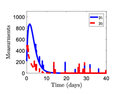
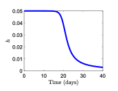
The effects from the other human societies on the main interactive society is modeled by a shot noise. Thus, the measurement noise is regarded as a non-Gaussian noise, which is a Gaussian noise that is affected by a shot noise as described in Eq. (3). In the simulation, the shot noise is seen as 20 impulses with magnitude of 200, which is randomly enforced to the measurement noise. This shot noise models the random entrance of 200 exposed and infected individuals from the other human societies into the human society of population 16000. Thus, the measurements (,) are affected by these 200 individuals during the simulation as shown in Fig. 2.
5.1 State estimation, tracking performance, and control effort
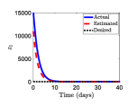
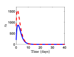
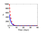
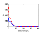
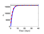
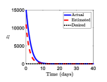
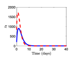
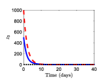
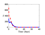
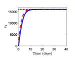
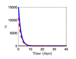
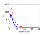
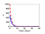
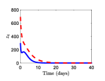
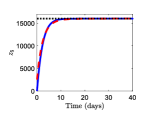
Figure 3 shows the state estimation performance for the influenza epidemics along with the convergence of populations and . It is seen that the proposed EMCKF algorithm is able to accurately estimate the state variables while only measuring the populations and . This accurate estimation is achieved when the shot noise is enforced to the measurement noise, which represents an impulsive random entrance of the exposed and infected populations to the main human society of 16000. This implies that the proposed estimation algorithm has a strong robustness when the system is perturbed by non-Gaussian noises.
Figure 3 also shows that the susceptible and infected individuals of the interactive human society are minimized in 14 days under the proposed control strategy. The convergence of variables and results in the convergence of populations and , and in turn the entire population is recovered. This implies that the proposed controller is able to recover all individuals of the human society with the population of 16000, even when the external infected individuals from other societies randomly invade the main society during a treatment time of 40 days. These results are in agreement with our main results presented in Section 4.2 and Theorem 2 based on which UUB/convergence of system’s errors is guaranteed.
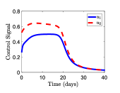
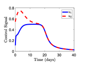
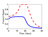
Figure 4 illustrates the rate of vaccination for susceptible individuals and the rate of antiviral treatment for the infected individuals . It is seen that the control signals generated by the proposed control technique fairly decreases to zero at the end of the treatment time. It can be also noted that none of the control signals hit the maximum control bound as the peak controls are and . Figure 4 also demonstrates the RCLF constraint violation during the simulation. It is seen that the RCLF violation is bounded by 0.05 when the relaxation coefficient is tuned as . A smaller value of relaxes the RCLF constraint and decreases the possibility of its conflict with the control bound constraint; however, smaller increases and in turn deteriorates the tracking performance. For higher relaxation coefficient , is relatively zero and the RCLF constraint is never violated, but the QP may be infeasible due to the conflict of the RCLF constraint with the control bounds. Thus, the penalty coefficient should be carefully selected to make a trade off between the tracking performance and the control constraints.
5.2 Robustness to parameter uncertainty
Different societies and populations can result in the influenza model (2.1) with different values of the system parameters . To evaluate the robustness of the proposed control scheme against the parameter perturbation, the system parameters are deviated by from their nominal values. Figure 5 illustrates the state estimation and tracking performance of the influenza epidemics when the system parameters are perturbed by . It is seen that the proposed EMCKF algorithm can still provide an accurate state estimation under either case. Under parameter perturbation, the number of susceptible and infected populations converges to a small ultimate ball around zero in 14 days using the proposed controller. In case that , although the estimated states and have a sluggish convergence to the actual states, the EMCKF algorithm can render a general convenient estimation performance. In this case, the convergence of and is also achieved in the same days as of and . This demonstrates that the proposed approach achieves good robustness against the parameter perturbation. These findings support the claim of our main results presented in Theorem 2 in which UUB/convergence of the tracking errors is ensured even in the presence of parameter uncertainties and state estimation error.
Figure 6 shows the control signals under parameter uncertainty. It is observed that the rate of vaccination for () under both cases and has relatively similar magnitude and behavior compared to in no perturbation case. Under both and , the maximum value of is . However, the rate of antiviral treatment for () under meets a higher magnitude in the first 10 days (), which is higher than in the case of no perturbation. Under , although hits the control bound during , convergence of is maintained. This implies that there is no conflict between the control bounds and the RCLF constraint such that they can be achieved at the same time. This demonstrates that the proposed approach is able to achieve convergence of system solutions and to satisfy the constraints in the presence of parameter perturbation and state estimation errors.
5.3 Superiority of the EMCKF algorithm over the ordinary EKF for the influenza epidemics

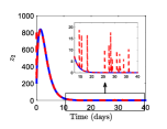
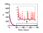
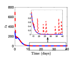
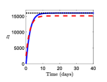
In this section, we highlight superiority of the EMCKF algorithm over the ordinary EKF when the system is affected by the shot noise introducing the random entrance of exposed and infected individuals from other societies to the society of interest. Figure 7 illustrates the state estimation and tracking performance of the influenza epidemic system under the proposed controller but when an ordinary EKF is employed. It is seen that the estimated states , , and contain unpleasant impulses stemming from the shot noise and in turn do not converge to their actual states. This results in a steady state estimation error for the state . Thus, it is seen that the estimation performance deteriorates when the system is disturbed by the shot noise and the EKF is employed.
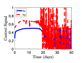
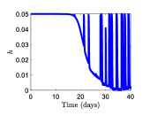
Since the proposed controller uses the estimated states, inconvenient state estimation of the EKF negatively impacts the generated control signals as shown in Fig. 8. Both the rate of vaccination for and the rate of antiviral treatment for intensively chatter after day 20 and even hits the control bound . This shows that improper estimation performance of the EKF in the presence of shot noise causes the control signal chattering, resulting in higher control cost. Figure 8 also shows that the RCLF constraint violation is not smooth and chatters after day 20. This demonstrates that the proposed controller can not preserve its robustness for an interactive human society (when the main human society is not isolated from the other societies i.e., existing of non-Gaussian noise) when the ordinary EKF is employed instead of the proposed EMCKF algorithm.
6 Discussion, Conclusions, and Future Work
6.1 Discussion
Control of influenza epidemics in a human society is an important global health concern that imposes economic and epidemiological burdens. The optimal control strategy is one of the most popular design approaches that has been employed to control the influenza epidemics. However, previous optimal control approaches have been designed with the assumptions of fully-known dynamics and fully-measurable states in addition to considering an isolated human society. The adaptive control strategy is an efficient design method for controlling the influenza epidemics in the presence of dynamic uncertainties. To cope with the modeling inaccuracies, an adaptive control method has been recently designed in [36] while still assuming that the system’s states are measurable and the human society is isolated. In addition, that controller did not take the optimality of the vaccination and antiviral treatment rates into account.
Since the influenza dynamic models are a set of nonlinear differential equations, the EKF is a convenient algorithm for the state estimation of such systems. However, since the human society of interest is not isolated from the other societies (it is an interactive society that is impacted by non-Gaussian noise), performance of the ordinary EKF deteriorates in the presence of other societies’ interactions.
6.2 Conclusions
Motivated by the aforementioned shortcomings of the existing works applied for the influenza epidemics and the aim of devising a new multi-objective controller for such systems, this paper presented a state estimation-based robust optimal control strategy for the influenza epidemics in an interactive human society in the presence of modeling uncertainties. An EMCKF algorithm was presented for state estimation purpose and a QP optimization problem was formulated w.r.t. a RCLF to recover the entire population of an interactive human society while compensating the state estimation error and the modeling error in an optimal fashion. The proposed QP-RCLF-EMCKF controller achieved multiple design specifications such as state estimation, tracking, control optimality, and robustness against the modeling error and the non-Gaussian noise stemming from the other societies’ effects. A Lyapunov stability argument was used to prove the boundedness of the susceptible and infected populations to a small neighborhood around the origin. The convergence of the error solutions was also discussed under a proper selection of the robust gain. This boundedness/convergence was achieved at minimal rates of the vaccination and antiviral treatment. Simulation results illustrated that the proposed approach is able to provide accurate state estimation, tracking performance, and robustness to the modeling inaccuracies and the non-Gaussian noise associated with the nature of the interactive human societies. This was achieved in an optimal control fashion.
6.3 Future works
The control strategy developed in this study can be modified to be employed for a wide range of epidemiological diseases such as tuberculosis [31], malaria [32], Hepatitis C virus (HCV) [24], HIV/AIDS [10], and COVID-19 [18]. In terms of future studies, the following items will be considered:
-
1.
In this paper, the system parameters have to be guessed for use in the controller. However, to relieve the engineer of the need for such guess, future work is planned to design an adaptation mechanism to estimate these unknown parameters.
-
2.
As illustrated in Figs. 3, 5, and 7, the exposed population peaks at the beginning of the simulation. It implies that the number of people who are infected with influenza but not yet infectious initially increases and then vanishes as time goes on. Future work is planned to design a controller such that the exposed population is maintained below a number during the treatment period.
These items naturally encourage us to extend the presented approach by estimating the system parameters and creating a safe control structure in which the exposed population is kept below a specified level.
References
References
- Ames et al. [2014] Ames, A. D., Galloway, K., Sreenath, K., & Grizzle, J. W. (2014). Rapidly exponentially stabilizing control lyapunov functions and hybrid zero dynamics. IEEE Transactions on Automatic Control, 59, 876–891.
- Ames et al. [2017] Ames, A. D., Xu, X., Grizzle, J. W., & Tabuada, P. (2017). Control barrier function based quadratic programs for safety critical systems. IEEE Transactions on Automatic Control, 62, 3861–3876.
- Arino et al. [2008a] Arino, J., Brauer, F., van den Driessche, P., Watmough, J., & Wu, J. (2008a). A model for influenza with vaccination and antiviral treatment. Journal of Theoretical Biology, 253, 118 – 130.
- Arino et al. [2008b] Arino, J., Brauer, F., van den Driessche, P., Watmough, J., & Wu, J. (2008b). A model for influenza with vaccination and antiviral treatment. Journal of Theoretical Biology, 253, 118 – 130.
- Azimi et al. [2017] Azimi, V., Munther, D., Fakoorian, S. A., Nguyen, T. T., & Simon, D. (2017). Hybrid extended kalman filtering and noise statistics optimization for produce wash state estimation. Journal of Food Engineering, 212, 136 – 145.
- Azimi et al. [2020] Azimi, V., Munther, D., Sharifi, M., & Vela, P. A. (2020). Enhancing produce safety: State estimation-based robust adaptive control of a produce wash system. Journal of Process Control, 86, 1 – 15.
- Azimi & Vela [2018a] Azimi, V., & Vela, P. A. (2018a). Performance reference adaptive control: A joint quadratic programming and adaptive control framework. In 2018 Annual American Control Conference (ACC) (pp. 1827–1834).
- Azimi & Vela [2018b] Azimi, V., & Vela, P. A. (2018b). Robust adaptive quadratic programming and safety performance of nonlinear systems with unstructured uncertainties. In 2018 IEEE Conference on Decision and Control (CDC) (pp. 5536–5543).
- Cinar & Principe [2012] Cinar, G. T., & Principe, J. C. (2012). Hidden state estimation using the correntropy filter with fixed point update and adaptive kernel size. In International Joint Conference on Neural Networks (pp. 1–6).
- Di Giamberardino et al. [2019] Di Giamberardino, P., Compagnucci, L., De Giorgi, C., & Iacoviello, D. (2019). Modeling the effects of prevention and early diagnosis on hiv/aids infection diffusion. IEEE Transactions on Systems, Man, and Cybernetics: Systems, 49, 2119–2130.
- Duan et al. [2013] Duan, W., Cao, Z., Wang, Y., Zhu, B., Zeng, D., Wang, F., Qiu, X., Song, H., & Wang, Y. (2013). An acp approach to public health emergency management: Using a campus outbreak of h1n1 influenza as a case study. IEEE Transactions on Systems, Man, and Cybernetics: Systems, 43, 1028–1041.
- Fakoorian [2016] Fakoorian, S. A. (2016). Ground reaction force estimation in prosthestic legs with an extended Kalman filter. Ph.D. thesis Cleveland State University.
- Freeman & Kokotovic [1996] Freeman, R., & Kokotovic, P. (1996). Robust Nonlinear Control Design. Birkhauser.
- Goldstein et al. [2009] Goldstein, E., Apolloni, A., Lewis, B., Miller, J. C., Macauley, M., Eubank, S., Lipsitch, M., & Wallinga, J. (2009). Distribution of vaccine/antivirals and the ‘least spread line’ in a stratified population. Journal of The Royal Society Interface, . URL: http://rsif.royalsocietypublishing.org/content/early/2009/10/09/rsif.2009.0393.
- Hao et al. [2015] Hao, G., li Sun, S., & Li, Y. (2015). Nonlinear weighted measurement fusion unscented Kalman filter with asymptotic optimality. Information Sciences, 299, 85 – 98.
- He et al. [2011] He, R., Zheng, W.-S., & Hu, B.-G. (2011). Maximum correntropy criterion for robust face recognition. IEEE Transactions on Pattern Analysis and Machine Intelligence, 33, 1561–1576.
- Hertzberg et al. [2018] Hertzberg, V. S., Weiss, H., Elon, L., Si, W., Norris, S. L., & Team, T. F. R. (2018). Behaviors, movements, and transmission of droplet-mediated respiratory diseases during transcontinental airline flights. Proceedings of the National Academy of Sciences, 115, 3623–3627.
- Ivorra et al. [2020] Ivorra, B., Ferrández, M., Vela-Pérez, M., & Ramos, A. (2020). Mathematical modeling of the spread of the coronavirus disease 2019 (covid-19) taking into account the undetected infections. the case of china. Communications in Nonlinear Science and Numerical Simulation, 88, 105303.
- Izanloo et al. [2016] Izanloo, R., Fakoorian, S. A., Sadoghi, H., & Simon, D. (2016). Kalman filtering based on the maximum correntropy criterion in the presence of non-Gaussian noise. In Annual Conference on Information Science and Systems (pp. 530–535). Princeton, New Jersey.
- Jiang et al. [2020] Jiang, K., Zhang, H., Karimi, H. R., Lin, J., & Song, L. (2020). Simultaneous input and state estimation for integrated motor-transmission systems in a controller area network environment via an adaptive unscented kalman filter. IEEE Transactions on Systems, Man, and Cybernetics: Systems, 50, 1570–1579.
- Jung et al. [2009] Jung, E., Iwami, S., Takeuchi, Y., & Jo, T.-C. (2009). Optimal control strategy for prevention of avian influenza pandemic. Journal of Theoretical Biology, 260, 220 – 229.
- Kalman [1960] Kalman, R. E. (1960). A new approach to linear filtering and prediction problems. ASME. J. Basic Eng., 82, 35–45.
- Khalil [2002] Khalil, H. K. (2002). Nonlinear Systems (3rd ed.). Upper Saddle River: Prentice Hall.
- Khodaei-Mehr et al. [2018] Khodaei-Mehr, J., Tangestanizadeh, S., Vatankhah, R., & Sharifi, M. (2018). Optimal neuro-fuzzy control of hepatitis c virus integrated by genetic algorithm. IET Systems Biology, 12, 154–161.
- Kim et al. [2016] Kim, J., Kwon, H.-D., & Lee, J. (2016). Constrained optimal control applied to vaccination for influenza. Computers & Mathematics with Applications, 71, 2313 – 2329.
- Lee et al. [2013a] Lee, J., Kim, J., & Kwon, H.-D. (2013a). Optimal control of an influenza model with seasonal forcing and age-dependent transmission rates. Journal of Theoretical Biology, 317, 310 – 320.
- Lee et al. [2013b] Lee, J., Kim, J., & Kwon, H.-D. (2013b). Optimal control of an influenza model with seasonal forcing and age-dependent transmission rates. Journal of Theoretical Biology, 317, 310 – 320.
- Lee et al. [2010] Lee, S., Chowell, G., & Castillo-Chávez, C. (2010). Optimal control for pandemic influenza: The role of limited antiviral treatment and isolation. Journal of Theoretical Biology, 265, 136 – 150.
- Liu et al. [2007] Liu, W., Pokharel, P. P., & Príncipe, J. C. (2007). Correntropy: Properties and applications in non-Gaussian signal processing. IEEE Transactions on Signal Processing, 55, 5286–5298.
- Liu et al. [2019] Liu, X., Ren, Z., Lyu, H., Jiang, Z., Ren, P., & Chen, B. (2019). Linear and nonlinear regression-based maximum correntropy extended kalman filtering. IEEE Transactions on Systems, Man, and Cybernetics: Systems, (pp. 1–10).
- Nematollahi et al. [2020] Nematollahi, M. H., Vatankhah, R., & Sharifi, M. (2020). Nonlinear adaptive control of tuberculosis with consideration of the risk of endogenous reactivation and exogenous reinfection. Journal of Theoretical Biology, 486, 110081.
- Rajaei et al. [2019] Rajaei, A., Vahidi-Moghaddam, A., Chizfahm, A., & Sharifi, M. (2019). Control of malaria outbreak using a non-linear robust strategy with adaptive gains. IET Control Theory & Applications, 13, 2308–2317.
- Reif et al. [2000] Reif, K., Gunther, S., E.Yaz, & Unbehauen, R. (2000). Stochastic stability of the continuous-time extended Kalman filter. IEE Proc. Control Theory Application, 147, 45––72.
- Samsuzzoha et al. [2013] Samsuzzoha, M., Singh, M., & Lucy, D. (2013). Parameter estimation of influenza epidemic model. Applied Mathematics and Computation, 220, 616 – 629.
- Sarkka [2007] Sarkka, S. (2007). On unscented Kalman filtering for state estimation of continuous-time nonlinear systems. IEEE Transactions on Automatic Control, 52, 1631–1641.
- Sharifi & Moradi [2017] Sharifi, M., & Moradi, H. (2017). Nonlinear robust adaptive sliding mode control of influenza epidemic in the presence of uncertainty. Journal of Process Control, 56, 48 – 57.
- Simon [2006] Simon, D. (2006). Optimal State Estimation: Kalman, H-infinity, and Nonlinear Approaches. John Wiley & Sons.
- Simon [2010] Simon, D. (2010). Kalman filtering with state constraints: a survey of linear and nonlinear algorithms. IET Control Theory & Applications, 4, 1303–1318(15).
- Song et al. [2021] Song, W., Wang, Z., Wang, J., & Shan, J. (2021). Particle filtering for a class of cyber-physical systems under round-robin protocol subject to randomly occurring deception attacks. Information Sciences, 544, 298 – 307.
- Tchuenche et al. [2011] Tchuenche, J. M., Khamis, S. A., Agusto, F. B., & Mpeshe, S. C. (2011). Optimal control and sensitivity analysis of an influenza model with treatment and vaccination. Acta Biotheoretica, 59, 1–28.
- Zhang et al. [2019] Zhang, Q., Shi, B., & Zhang, Y. (2019). Conditional importance sampling for particle filters. Information Sciences, 501, 388 – 396.