Dynamical evolution of cosmic supermassive binary black holes and their gravitational wave radiation
Abstract
We investigate the evolution of supermassive binary black holes (BBHs) in galaxies with realistic property distributions and the gravitational-wave (GW) radiation from the cosmic population of these BBHs. We incorporate a comprehensive treatment of the dynamical interactions of the BBHs with their environments by including the effects of galaxy triaxial shapes and inner stellar distributions, and generate a large number of BBH evolution tracks. By combining these BBH evolution tracks, galaxy mass functions, galaxy merger rates, and supermassive black hole–host galaxy relations into our model, we obtain the statistical distributions of surviving BBHs, BBH coalescence rates, the strength of their GW radiation, and the stochastic GW background (GWB) contributed by the cosmic BBH population. About 1%–3% (or ) of supermassive BHs at nearby galactic centers are expected to be binaries with mass ratio (or ). The characteristic strain amplitude of the GWB at frequency is estimated to be , and the upper bound of its results obtained with the different BH–host galaxy relations can be up to , which await testing by future experiments (e.g., the Square Kilometer Array, FAST, Next-Generation Very Large Array). The turnover frequency of the GWB spectrum is at . The uncertainties on the above estimates and prospects for detecting individual sources are also discussed. The application of the cosmic BBH population to the Laser Interferometer Space Antenna (LISA) band provides a lower limit to the detection rate of BBHs by LISA, .
Subject headings:
Astrodynamics (76); Gravitational waves (678); Cosmological evolution (336); Galaxy dynamics (591); Galaxy mergers (608); Galaxy nuclei (609); Gravitational wave astronomy (675); Supermassive black holes (1663)1. Introduction
In the modern paradigm of hierarchical galaxy formation and evolution, a natural consequence of mergers of galaxies with central supermassive black holes (SMBHs, hereafter BHs) is the formation of supermassive binary black holes (SMBBHs, hereafter BBHs) at galactic centers (e.g., Begelman et al. 1980; Yu 2002; Benson et al. 2010). The formed binaries interact with surrounding stars and gas, which may distinguish the systems with some unique astronomical phenomena different from those with only one BH. If the separation of the two BHs can decay to be sufficiently close through the interactions, significant gravitational waves (GWs) will be radiated, taking away energy and angular momentum, leading to mergers of the BBHs, and contributing to the GW background (GWB) at the relatively low-frequency band [e.g., the detection frequency bands of the Pulsar Timing Array (PTA) experiments (Hobbs, 2013; McLaughlin, 2013; Desvignes et al., 2016; Verbiest et al., 2016), Laser Interferometer Space Antenna (LISA; https://www.lisamission.org), and Taiji/Tianqin (Ruan et al., 2019; Wang et al., 2019)]. Studies of the strength of the GW radiation caused by BBH mergers, the characteristics of BBH systems and their statistical properties, would provide an important probe to the hierarchical structure formation and evolution model, BH physics, and the gravitation theory.
In this work, we investigate the expected statistical distributions of BBHs surviving in the nearby universe and the strength of the GWs radiated by merging BBHs. To determine how many BBHs can survive or coalesce, the dynamical evolution timescales of BBHs play a vital role. For example, Yu (2002) shows that the evolution of BBHs in a gas-poor system depends on BH mass ratio and host galaxy type. BBHs with very low mass ratios (say, ) are hardly formed by mergers of galaxies, because the dynamical friction timescale is too long for the smaller BH to sink into the galactic center within a Hubble time. For BBHs with moderate mass ratios, one essential factor to determine their evolution timescales is how many stars can pass by the vicinity of the BBH to interact strongly with the BBH and make it lose energy, and it has been shown that BBHs in low-dispersion galaxies or in highly flattened or triaxial galaxies have relatively low evolution timescales (Yu, 2002). Over-simplified treatments on the interaction of a BBH with its environments may lead to some uncertainty in the current estimation of the strength of the GW radiation emitted by the BBHs, as the interactions affect how many BBHs are surviving at a given separation, and when and where gravitational radiation becomes dominant in making a BBH lose energy; and a realistic treatment of the BBH interaction with their environments is necessary for the BBH dynamical evolution models and the GW radiation estimation (Shannon et al., 2015; Arzoumanian et al., 2016; Lentati et al., 2015). To obtain the coalescence rate of merging BBHs in the realistic universe and the realistic statistical distribution of surviving BBHs, in this work we model the dependence of the BBH dynamical evolution on stellar distributions and galaxy shapes, and we incorporate the BBH dynamical evolution model with the realistic distributions of galaxy properties (e.g., stellar distributions, galaxy shapes, galaxy merger rates).
This paper is organized as follows. In Section 2, we review the dynamical processes and the model for the evolution of a BBH in gas-poor systems. The detailed model is mainly adopted from Yu (2002). In Section 3, we describe the modeling of the distribution of surviving BBHs, BBH coalescence rates, and the strength of stochastic GWB. In Section 4, we describe the galaxy samples, the realistic galaxy distributions and the galaxy merger rates used in the model. In Section 5, we present our results for the distribution of surviving BBHs and the GW strength radiated by merging BBHs. Discussion is given in Section 6 and conclusions are given in Section 7.
2. Orbital evolution of BBHs
In a gas-poor galaxy merger, the formation and evolution of a BBH can be divided into the following stages, according to the dominant physical mechanisms that act to drain the energy of the orbit of two BHs (Begelman et al., 1980; Yu, 2002). The relative importance of each mechanism is determined by the spatial scale of the separation between the two BHs. (1) Dynamical friction stage: after two galaxies merge, each BH in its progenitor galaxy will sink into the center of the common potential well of the merging galaxy, due to dynamical friction, from a separation of several tens of to . (2) Non-hard binary stage: the two BHs with masses and () form a bound system with semi-major axis
| (1) | |||||
where , is the one-dimensional velocity dispersion of the merged galaxy core. The dynamical friction continues to make the BBH lose energy but becomes less and less effective as the binary orbital velocity increases and its orbital period decreases. Meanwhile, from time to time a star walks to the vicinity of the BBH and the three-body interactions between the BBH and the stars gradually become the dominant mechanism to make the BBH lose energy. This stage is an intermediate stage between the previous dynamical friction stage and the next hard binary stage. (3) Hard binary stage: the BBH becomes hard when its semi-major axis
| (2) | |||||
A hard binary loses energy mainly by interacting with stars passing in their vicinity, most of which will be expelled from the BBH with an energy gain after one or more encounters with it. In such expulsions, the relative change in the BBH orbital energy is independent of the energy (Heggie, 1975), which can simplify the analysis of the BBH evolution timescale at this stage. (4) Gravitational radiation stage: when the semimajor axis of the BBH is small enough (e.g., ), gravitational radiation becomes the dominant effect to drive the BBH orbital decay. This stage is likely to occur before the BBH becomes hard if .
In this paper, we obtain the orbital evolution of a BBH by following the model presented in Yu (2002), supplemented with a numerical method to calculate the stellar orbital motion and obtain the stars that can move to the vicinity the BBH in triaxial gravitational potentials. We summarize the model of the evolution timescales of the BBH at the four stages in Section 2.1-2.4, respectively. Note that the evolution of the BBHs at the non-hard and the hard stages is critical to determine how the BBHs are distributed at pc and sub-pc scales, and when and where the gravitational stages start. One essential factor to determine the BBH evolution timescales in those stages is how many stars on low-angular momentum orbits, which can pass through the vicinity of the BBH, are available to interact strongly with the BBH. Even if the low-angular momentum stars initially in the stellar system are expelled away by interactions with the BBH, the stars on high-angular momentum orbits can still move onto low-angular momentum orbits by the two-body relaxation or by orbital precession in non-spherical (e.g., flattened or triaxial) gravitational potentials (Magorrian & Tremaine, 1999; Yu, 2002; Berczik et al., 2006; Khan et al., 2011; Preto et al., 2011; Khan et al., 2013; Vasiliev et al., 2015). In this work, we include the effect of the non-spherical potentials, as well as that of the two-body relaxation. We define a “loss region” by the (specific energy, specific angular momentum) phase space of the stars that can precess onto low-angular momentum orbits with pericenter distances . The stars in the loss region can pass by the BBH vicinity and then escape from the BBH after strong interactions with it. We obtain the loss region by numerical simulations, and the method is described in Section 2.5.
In the model, we assume that the BHs are on nearly circular orbits and ignore their eccentricity evolution at the least for the following reasons. (1) At the dynamical friction stage, the orbital decay of a star cluster or a secondary BH generally does not result in a highly eccentric orbit when the two BHs become bound (Polnarev & Rees, 1994). (2) If the BBH eccentricity when the two BHs become bound is small (e.g., ), Quinlan (1996) shows that the BBH eccentricity hardly grows as the BBH hardens. (3) The BBH eccentricity decays quickly at the gravitational radiation stage (Peters & Mathews, 1963; Baker, 2006). (4) In kinematically anisotropic spherical systems with stars mostly counter-rotating with the BBH orbit, some simulations show that the BBH eccentricity could increase significantly (Amaro-Seoane et al., 2010; Sesana et al., 2011; Holley-Bockelmann & Khan, 2015), however it is expected that the significant increase in BBH eccentricity can be decreased or erased if the systems are triaxial, by applying the same reasoning as for the alignment-erasing effect obtained in Cui & Yu (2014). (5) Evolution of triple or multiple BHs can result in BBHs with extreme eccentricity; however, the contribution of those cases to the stochastic GWB at the PTA bands is shown to be insignificant (see the left panel of Fig. 4 in Bonetti et al. 2018). (6) It was suggested that a significant fraction of BBHs should have extreme eccentricities close to 1 so that the strength of gravitational waves radiated by mergers of those BBHs can be relatively low (e.g., see Fig. 1 in Chen et al. 2016), in order to relieve the tension between the non-detection of the stochastic GWBs and the model expectation. According to the results of this work below, the assumption of BBHs with extreme eccentricities are not necessarily required. In addition, exploration on detection prospects for individual BBH sources specifically with extreme eccentricities formed in special conditions are beyond the scope of this work.
In the model, the evolution of the BBH orbital semimajor axis is described by or , where is the orbital semimajor axis of the BBH or the separation of the two BHs (if they are not bound, yet), is the cosmic time, and is the period since an event at cosmic time (e.g, galaxy merger). The BBH evolution timescale at a given is defined by
| (3) |
where .
At the dynamical friction stage, comes mainly from the contribution of dynamical friction, and we denote the corresponding evolution timescale by the dynamical friction timescale . After the BBH becomes bound, if we only include the contribution of gravitation radiation to , the corresponding evolution timescale is denoted by (see Eq. 11 below); and if we only include the contribution of the BBH interaction with stars to , the corresponding evolution timescale is denoted by the BBH hardening timescale . We obtain the BBH evolution timescale after the BBH becomes bound by
| (4) |
We have at the non-hard and the hard stages and at the gravitational radiation stage.
2.1. Dynamical friction stage
In the dynamical friction stage, each of the BHs sinks into the common center of the merger remnant independently. We carry out a simple analysis of the evolution timescale at the dynamical friction stage. Assume that a BH of mass is located at the center of a spherical galaxy with stellar mass density and one-dimensional velocity dispersion . Suppose that a BH with mass that used to be at the center of a galaxy is orbiting with a velocity and spiraling into the center of the parent galaxy by dynamical friction. Because the in-spiraling BH is accompanied by the stars bound to it with total mass , dynamical friction brings the two BHs together much more rapidly than if is naked (Milosavljević & Merritt, 2001; Yu, 2002). The dynamical friction exerts on and its accompanying stars and decelerate them at a rate given by
| (5) | |||||
where , , erf is the error function, and the logarithm of the ratio of the maximum and the minimum impact parameter is set to unity.
The mass of the stars bound to the secondary BH can be estimated as follows. In the potential of the spherical galaxy with central BH , the stars around the BH is tidally truncated at the radius
| (6) | |||||
where and are the circular frequency and epicycle frequency in the parent galaxy. If the stars surrounding each of the BHs follow a singular isothermal distribution, and their one-dimensional velocity dispersions and , respectively, we have , and . By applying them into Equation (6), we have , and the total mass of the stars bound to the BH is given by
| (7) |
We follow equations (40)-(42) in Yu (2002) to obtain the BBH evolution timescale at the dynamical friction stage .
2.2. Non-hard binary stage
The BBH orbital decay in the non-hard binary stage comes from both dynamical friction from distant stars and three-body interactions between the BBH and the stars passing the BBH vicinity. As done in Yu (2002), we apply the dynamical friction timescale to estimate the BBH hardening timescales at the non-hard binary stage, because scattering experiments with the restricted three-body approximation basically give a hardening timescale similar to the application of the dynamical friction timescale (Quinlan, 1996).
Stars may gain energy and be removed from the galactic core by interactions with the BBH. Before the BBH becomes bound, the stellar mass removed from the galactic core due to the BH orbit decay can be ignored. During the non-hard binary stage, the depletion of the stars can be significant in some galaxies. Before the BBH becomes hard, if the mass of the initial stellar population in the loss region is not sufficient, the BBH would lose energy mainly by dynamical friction with distant stars (which becomes more and more inefficient as the BBH hardens) and by three-body interactions with the low-angular-momentum stars diffused from high-angular-momentum orbits by two-body relaxation (which will dominate the BBH hardening timescales in the hard binary stage). Thus the BBH hardening timescale should be higher than those estimated from and smoothly increase to connect the hardening timescale in the hard binary stage. We use the linear approximation to obtain the BBH hardening timescale at :
| (8) |
where is the semimajor axis where the initial population of stars in the loss region are all removed from the loss region, is obtained from Section 2.1, and is obtained from Section 2.3.
2.3. Hard binary stage
In the hard binary stage, the orbital decay of a BBH is mainly driven by three-body interactions with low-angular-momentum stars passing its vicinity. The BBH orbital decay timescale is mainly determined by how many stars are available to move onto low-angular-momentum orbits and how fast they can move onto the orbits to strongly interact with the BBH. After such strong interactions, the stars escape with energy gain and are considered to be cleared from the loss region. We denote the orbital binding energy of a star per unit mass by . Assuming that is the number clearing rate from the loss region for stars with energy and is the corresponding average change of the specific energy of the stars escaping from the BBH during an interaction with the BBH, the orbital energy loss rate of the BBH is given by
| (9) |
where is the orbital energy of the BBH, is the reduced mass of the BBH, is the mass of a single star, and all stars are assumed to have the same mass. The quantity is only weakly dependent on for hard binaries. Hence we assume where is a constant which is determined from the numerical experiment of Quinlan (1996). Therefore, after the BBH becomes hard, its hardening timescale due to stellar interaction is given by
| (10) |
where is the mass of a star and is assumed to be a solar mass in this work. We obtain the clearing rate by following the analysis in section 3.2 in Yu (2002), which is affected by the size of the loss region and the two-body relaxation processes.
2.4. Gravitational radiation stage
In the gravitational radiation stage, the evolution timescale of the BBH is described by
| (11) |
where is the orbital eccentricity of the binary (Peters, 1964) is set to zero in this work as argued above. The transition from the evolution stages of the BBH interacting with its surrounding environments (the hard binary and non-hard binary stages) to the gravitational radiation stage can be marked by . At , the BBH GW frequency and the orbital period are labeled by and , respectively.
Note that a large eccentricity can not only make the BBH enter the gravitational radiation earlier, but also accelerate the orbital decay, and the gravitational radiation energy spectrum can be correspondingly changed.
2.5. Loss region
The size of the loss region in the phase space depends on galaxy shapes. The loss region in a spherical stellar system is a ‘loss cone’ given by
| (12) |
( is a dimensionless factor ). In an axisymmetric or triaxial system, there exist centrophilic orbits such as box orbits, which pass arbitrarily close to the center and have low angular momentum, as well as centrophobic orbits such as loop or tube orbits, which avoid the center and have high angular momentum. We use a characteristic specific angular momentum to mark the transition from centrophilic () to centrophobic () orbits. The loss region in an axisymmetric system can be approximated as a ‘loss wedge’ where stars on centrophilic orbits with can precess into the loss cone, while those on centrophobic orbits with cannot. In a triaxial system, the loss region can be approximated by in which most of the stars can precess into the loss cone.
In this work, we obtain by numerically simulating the motion of a star under the combined gravitational potential of a central point mass and the galactic stars (see eq. 7 in Cui & Yu 2014). The galactic potential is spherical if it can be described in the form and triaxial if it can be described in the form . If the shape distribution of host galaxies is described in mass density, we use the following equation (which is derived for logarithmic potentials) to approximately convert it into the shape distribution in gravitational potentials:
| (13) |
where represents the medium-to-major or the minor-to-major axis ratio in the density shape, and represents the corresponding ratio in the potential shape (see Eq. 2.72b in Binney & Tremaine 2008). If , we have .
Noting that it is time-consuming to obtain in a large number of galaxies by numerically tracing the motion of each star in a galaxy for a sufficiently long time to judge whether it can move to the center on a centrophilic orbit, we improve the judging efficiency for a centrophilic orbit and describe the method to obtain below.
In a general triaxial system, for a centrophilic orbit, the motion of the stars can pass arbitrarily close to the center, and the stellar orbital angular momentum will flip its direction during the orbital motion. Numerically we count a star as one in the loss region, if all the three , , and components of its orbital angular momentum flipped their directions. This criterion is effective and efficient enough in practice, although in principle the stars that change the signs of their orbital angular momentum components are not exactly the same population of the stars that can move to the center (on centrophilic orbits). Given the potential of a merger remnant, we obtain the characteristic angular momentum as a function of the binding energy . In practice, only stars in a certain range of have considerable importance to the three-body interactions with a BBH. We set the boundaries of as , where and . For each system, we obtain for values of equally spaced within the given range. For each , we use the Monte Carlo method to generate test particles whose squared angular momenta are uniformly distributed in with isotropic velocity distributions, where is the specific angular momentum of a circular orbit at . We follow the evolution of these test particles within the potential of the host merger remnant, which is composed of two parts, i.e., the potential from the BBH and the galactic potential from the host galaxy, where the potential of the BBH is simplified as a Keplerian potential around a point mass and the galactic potential is assumed to be triaxial. We calculate the fraction of the test particles that flipped the signs of all the , , and components of the orbital angular momentum during an evolution time of , where is the period of a circular orbit at energy . The characteristic angular momentum is then obtained by . The above method to obtain is efficient enough.
We have done some tests to show that the above method is effective, although the stars that change the signs of their orbital angular momentum components are not exactly the same population stars that can move to the center and the evolution of the orbital angular momentum of a star is traced with an evolution time of only . The tests are done for the galaxies (with a limited number ) randomly selected from the mock galaxy sample (with the shape distribution in Padilla & Strauss 2008) presented in Section 4.2. In each galaxy, the motions of 500 stars at a given are traced for a sufficiently long time (), where the two values of and are tested. Our tests show that the number ratios of the stars that change the signs of their orbital angular momentum components to the stars that can move the center is close to and the extension of the evolution time of a star does not affect our results significantly.
As mentioned above, in a configuration close to being axisymmetric, the loss region is approximated as a loss wedge, and the obtained by the above method may be too low and is not appropriate to be taken as the defined in the loss wedge, as a star is recognized as being in the loss region only if all the three , , and components of its angular momentum flipped their directions during the orbital evolution. We estimate the size of the loss wedge by the following criterion: a star is recognized as being in the loss wedge if at the least one (but not all) of the three , , and components of its angular momentum flipped their directions and the remaining components possess a combined specific angular momentum smaller than (where is set to in Eq. 12, i.e., the values of with . We calculate the fraction of the stars satisfying the above conditions, and the characteristic angular momentum in the loss wedge is then obtained by .
Given a shape configuration of a system, we use the above methods to numerically estimate both the size of the loss region by applying the criterion for a general triaxial system and the size of the loss wedge by applying the criterion for an axisymmetric system, and the stars in the loss wedge and in the loss region both contribute to the stellar reservoir to have strong interactions with the BBH.
In the model, for simplicity, we do not consider the time evolution of galaxy shapes (e.g., rotation of a triaxial system or changes in axis ratios) 111Some possible effects of the changes in axis ratios can be partly inferred from this work done by adopting three different sets of the galaxy triaxial shape distributions and comparing their results. Regarding the rotation of a triaxial system, the characteristic rotating pattern timescale is generally much longer than one orbital period of a star with the relevant energy, but it can be shorter than the timescale of the star on a centrophilic orbit to precess into the loss cone. The assumption of ignoring the shape rotation is plausible and does not affect the above estimate of much if the stellar centrophilic orbits in the triaxial system are mostly stochastic (which generally have relatively large apocenter distances and low ; cf. the right panel in Figure 4 of Magorrian & Tremaine 1999). The shape rotation may affect the above estimate of if the precessions of the stellar orbits into the loss cone are regular, which needs a further detailed complement for its statistical effect; nevertheless, an extreme case of fast rotation of a triaxial system would result in the dynamical effects partly close to those in axisymmetric systems, and the effects in axisymmetric systems can be partly seen from the results obtained from one of the three observational galaxy shape distribution adopted in this work (i.e., Weijmans et al. 2014, which prefers the axisymmetric shape configurations). and the difference of galaxy shapes at different galactic radii.
3. Modeling of the distributions of merging BBHs and surviving BBHs
3.1. Distributions of surviving BBHs
We define the distribution of surviving BBHs by () so that is the comoving number density of BBHs at redshift with total mass in the range , mass ratio in the range , and semimajor axis (or separation) in the range .
We define the galaxy stellar mass function (GSMF) by so that is the comoving number density of galaxies with mass in the range at redshift . We describe the galaxy merger rate per galaxy at redshift by () so that represents the average number of galaxy mergers with mass ratio in the range within time for a descendant galaxy with mass , where is the corresponding cosmic time at redshift . Similarly as the above definition for galaxies, we also define the corresponding variables for the spheroidal components of merging remnants. (which are also called “bulge” for simplicity and denoted by the subscript ∗ below), i.e, the stellar mass function , the merger rate per spheroidal component , and the mass ratio . For major mergers, we assume that galaxy mergers form spheroids characterized by mass and merger mass ratio . For minor mergers, the secondary galaxy is assumed to be accreted onto the spheroidal component of the primary galaxy, and the mass of the spheroidal component of the merging remnant is assumed to be the sum of the stellar masses in the secondary galaxy and in the spheroidal component of the primary galaxy, and the merger mass ratio is their mass ratio.
We connect the BBH distribution function with the galaxy merger rate by the following equations:
| (14) |
and
| (15) |
where is a probability function defined so that represents the probability that a galaxy merger characterized by the bulge mass of the merging remnant and mass ratio at redshift leads to a BBH with total mass in the range and mass ratio in the range , is a probability function defined so that represents the probability that the galaxy merger leads to a BBH with semimajor axis in the range at a time after the galaxy merger, is the probability that a galaxy merger with total mass and mass ratio at redshift results in the merging remnants characterized by and , and , , and . The distributions of and depend on BH demography and galaxy demography, and the distribution of depends on the distribution of the intrinsic structure of galaxies. As to be seen below, the BBH mergers contributing to the GWB comes mainly from redshift . The distribution of the intrinsic structure of galaxies and BH demography used in this work are mainly based on observations in the nearby universe, and we assume that they are independent of redshift at low redshift and then distributions of and are independent of redshift in this work. The function is obtained by assuming that the BBH evolves independently inside the merging galaxy remnant and that no other later galaxy mergers affect the BBH evolution. However, before the BBH reaches the gravitational radiation stage, it is possible that the host merger remnant undergoes a big impact, that is, a major merger with another galaxy or being accreted by another bigger galaxy to become a satellite galaxy in this work; in these cases the interactions of triple or multiple BHs may lead to quick BBH coalescence or BH kicks out of the host merger remnant. The function () is introduced in Equation (14) to represent the probability that the host merger remnant does not experience such big impacts from redshift to . The detailed method to obtain is described in Section 3.4. In this work, the effects of the big impacts (e.g., on the surviving BBH distributions, BBH coalescence rates, GWBs; see also Eqs. 21 and 31 below) are included by removing a corresponding BBH system from consideration if it experiences a big impact during its evolution, and we neglect the contribution from possibly newly formed BBHs caused by triple or multiple BH interactions.
As to be shown below, we use Monte-Carlo simulations to generate galaxy mergers and calculate the BBH evolution in the galaxy mergers. Suppose that we have galaxy mergers with parameters leading to the formation of BBHs with parameters () and semimajor axis () at a time after the galaxy mergers. The probability function can be obtained by
| (16) |
By applying Equation (16) into Equation (14), we have
| (17) |
where
| (18) |
is the BBH evolution timescale at (see Eq. 3), is the solution of equation , is a step function defined by if and if , and is the corresponding redshift of cosmic time .
In a simplified or extreme case, if with being a constant, and the BBH evolution () is the same for the same (), Equation (17) is simplified as
| (19) |
3.2. BBH coalescence rates
We define the BBH coalescence rate so that represents the comoving number density of the BBH coalescence events occurring during cosmic time and with the total mass of the two coalescing BHs in the range and their mass ratio in the range . The BBH coalescence rate can be obtained by
| (20) |
where represents the fraction of the BBHs that can coalesce before cosmic time among those BBHs with parameters caused by galaxy mergers with parameters occurring at redshift . The fraction of can be obtained by
| (21) |
where the term removes the contribution of a BBH system if it experiences a big impact before its expected coalescence time obtained by assuming it evolves independently.
In the extreme case used for Equation (19), if , Equation (22) is simplified as
| (23) |
The above equation can be further simplified in the following two cases.
- •
-
•
If the BBH coalescence occurs immediately after a galaxy merger (i.e., ), Equation (23) is simplified as
(25) and the BBH coalescence rate can be approximately obtained from the galaxy merger rate at the same redshift.
3.3. Stochastic gravitational-wave background
We denote the total present-day energy density in gravitational radiation by , which can be expressed by
| (26) |
where is the speed of light, is the gravitational constant, is the frequency of gravitational waves observed today on earth, and is the characteristic strain amplitude of the GW spectrum over a logarithmic frequency interval (Phinney, 2001).
The present-day GW energy density can be obtained by an integration over the contribution from the GW radiation sources (BBHs in this work) in the cosmic history as follows,
| (27) |
where is the frequency of the GW signal in the source’s cosmic rest frame and is related with through , is the GW energy per unit time radiated by an in-spiraling BBH with parameters (see the definition of in Eq. 11), and the term accounts for the redshift of the GWs since emission.
During the in-spiral, the frequency of the GW signal is twice the Keplerian orbital frequency of the BBH and increases monotonically till the final coalescence and can be estimated by
| (28) |
The upper limit of when the circular in-spiral assumption in Equation (32) is valid can be roughly estimated by twice of the Keplerian orbital frequency at the innermost stable circular orbit (ISCO) for a Schwarzschild BH with mass the same as the total mass of the BBH, that is,
| (29) |
The above upper limit for BBHs is safely outside the frequency band probed by PTAs.
3.4. Multiple galaxy mergers during the evolution of a BBH
In this subsection, we present a rough way on how to obtain the function shown in Equation (14), the probability that the host merger remnant does not experience big impacts (including major mergers with other galaxies and mergers with bigger galaxies) from redshift to .
We define the progenitor galaxy merger rate per galaxy at redshift by so that represents the average number of mergers of a galaxy with mass undergoing with a second galaxy with mass within during time . We define , and thus . The function can be obtained from the GSMF and the descendant galaxy merger rate (see their definitions in Section 3.1) through the following equation on the number of the galaxy merger events per unit comoving volume:
| (35) |
where , and the factor of accounts for the symmetry between and in the definition of the progenitor merger rate; and thus we have
where . The average number of big impacts that a host merger remnant with mass is expected to go through between redshifts and ()is given by
| (37) | |||||
where is the lower limit of the mass ratios for major mergers, and . The probability that the host merger remnant keeps intact between redshifts and , can be given by
| (38) | |||||
which is reduced to 1 if and 0 if .
For major mergers of galaxies, whose merging remnants are spheroids, the term in Equation (14) can be obtained by replacing directly with in the function obtained in Equation (14). For minor mergers of galaxies, we also do this replacement, which is a rough approximation and deserves further improvements.
4. Galaxy distributions, SMBH demography, and galaxy merger rates
In this section, we present the galaxy samples, the realistic galaxy distributions, the galaxy merger rates, and the BH-host galaxy relations used in the model. We also describe the BBH evolution tracks obtained with those distributions.
We generally use a cosmology model with parameters , , , , and (Planck Collaboration et al., 2016). The results of some previous works adopted by our model may have some differences in their used cosmological models. For example, the GSMF adopted from Behroozi et al. (2019) is obtained with a cosmology model with parameters as mentioned above, and the galaxy merger rates adopted from Rodriguez-Gomez et al. (2015) is obtained with a cosmology model with parameters , , , , and (Hinshaw et al., 2013). In this work, it is plausible to assume the differences in our conclusions caused by the different versions of the cosmological models are negligible. We use the results from the previous works directly without doing conversion between the different cosmological models, except that they are converted to the values with .
4.1. Observational galaxy surface brightness and triaxial shape distributions
To model the dynamics of BBHs inside galaxy merger remnants, the stellar density distributions of the host remnants are needed. To construct a sample of host galaxy merger remnants with a realistic stellar distribution, we use the early-type galaxies obtained in the survey (Cappellari et al., 2011) and in Lauer et al. (2007a), both of which have high spatial resolution (Hubble Space Telescope) imaging to detect the inner part of the stellar surface brightness distributions, as described in Section 4.1.1. Regarding the intrinsic triaxial shape distributions of galaxies, we use the observational results summarized from the survey and the Sloan Digital Sky Survey (SDSS), as described in Section 4.1.2.
4.1.1 Observational galaxy surface brightness distributions
The survey is based on a volume-limited sample of nearby () early-type galaxies, with multi-band imaging as well as two-dimensional bulk kinematic information as derived from the optical integral-field spectroscopy. Among these early-type galaxies, were found to have archive data (Krajnović et al., 2013). In the compilation of Krajnović et al. (2013), galaxies show strong dust features in the nuclei and are thus excluded from the analysis. The surface brightness of the remaining galaxies, which are observed by surveys are all converted to the band (broad-band ), in order to make comparison with previous studies. The “Nuker law” profile (Lauer et al., 1995) is used to fit the surface brightness of these galaxies, i.e.,
| (39) |
where is the surface brightness at the break radius , and are the asymptotic inner and outer slopes of the surface brightness profile, respectively, and parameterizes the sharpness of the break. Cappellari et al. (2013) provides the mass-to-light ratio in the band for the galaxies. which is obtained by the best-fitting self-consistent Jeans Anisotropic Multi-Gaussian Expansion model. Note that the five Nuker-law parameters are obtained in the band, whereas the above mass-to-light ratios are obtained in the SDSS band. We convert the from the band to the band as follows, based on the magnitude differences in the two bands. Cappellari et al. (2013) provides the total SDSS -band luminosities for these galaxies. Among the 122 galaxies adopted in our study, 53 have the -band apparent magnitudes and all of them have the -band apparent magnitudes. For the 66 galaxies without the -band magnitudes but with the SDSS ones, we convert their -band apparent magnitudes to the -band ones, based on one empirical equation, listed in http://www.sdss3.org/dr8/algorithms/sdssUBVRITransform.php (see also Jester et al. 2005). For the remaining 3 galaxies without the -band and the SDSS - and -band magnitudes, we do the conversion by (e.g., Lauer et al. 2007a). The absolute magnitudes can be converted from their apparent magnitudes, given the distances and the extinctions of these galaxies (listed in Table 3 of Cappellari et al. 2011), by assuming the extinction ratio (Table 3.21 in Binney & Merrifield 1998).
Lauer et al. (2007a) provide the “Nuker law” parameters , , , , and together with some other parameters for a sample of galaxies, which are compiled from several investigations of the central structure of early-type galaxies. The mass-to-light ratio of these galaxies can be estimated according to the following empirical galaxy scaling relation in the V-band (Magorrian et al., 1998):
| (40) |
where is the galaxy luminosity in the V-band.
In Figure 1, we show the galaxy sample (blue) and the Lauer et al. (2007a) sample (red) in the six-dimensional parameter space composed of the five “Nuker law” parameters (i.e., break radius , surface brightness at break radius , , , ) and the mass-to-light ratio in the band. In the figure, the mass-to-light ratios of the Lauer et al. (2007a) sample are estimated by Equation (40). There are 61 common galaxies in the two samples, and the fit parameters of the same galaxies may be different in the two samples, which are all shown in Figure 1.
4.1.2 Observational galaxy triaxial shape distributions
The triaxial shape of a galaxy can be characterized by the two parameters, i.e., the medium-to-major axis ratio and the minor-to-major axis ratio , where , , and represent the major, the medium, and the minor axis of an iso-density layer of the galaxy, respectively. The triaxial shape can also be described by an equivalent set of parameters i.e., the triaxiality and the minor-to-major axis ratio . The general triaxial description can be reduced to the following special cases: spherical shape with , oblate spheroid with , and prolate spheroid with .
In the left panel of Figure 2, we show the shape distributions of early-type galaxies obtained from observations. The results obtained from the photometric study in the SDSS indicate that early-type galaxies are better described by triaxial shapes than by purely spheroidal shapes. As shown in the figure, the green plus symbol marks the possible range of the mean medium-to-major and minor-to-major axis ratios of the early-type galaxies in the SDSS DR3 data set (Vincent & Ryden, 2005). The blue and red contours indicate the two-dimensional axis ratio distribution of early-type galaxies in the SDSS DR6 data set (Padilla & Strauss, 2008) and the SDSS DR8 data set (Rodríguez & Padilla, 2013), respectively. The results obtained from the galaxy sample, where both the photometric and the bulk kinematic information are used, show that early-type galaxies can be classified by fast- and slow-rotators (Emsellem et al., 2007; Krajnović et al., 2011). The magenta color-bar marks the mean and the standard deviation of the minor-to-major axis ratios for a nearly oblate fast-rotator galaxy sample from the galaxy survey, obtained through a triaxial configuration fitting (Weijmans et al., 2014) (where the mean values of and are and , respectively, and their standard deviations are and , respectively). The shape parameters cannot be well constrained for the slow-rotator galaxies, due to the limited sample size and the lack of a clearly defined projected rotation axis in many of the systems.
We will apply the different shape distributions to our study and see how different the results are affected by them.
4.2. Mock galaxy sample
As the observational sample size shown in Figure 1 is small, we construct a mock galaxy sample with a larger size for the statistical study of the BBH evolution in galaxies with realistic property distributions. The mock galaxy sample is generated based on all the galaxies shown in Figure 1 and follow the statistical distributions of their properties. For each galaxy in the mock galaxy sample, we first select a galaxy, e.g., galaxy with parameters , randomly from Figure 1, then add small scatters to the corresponding parameters and assign the new parameter set to the galaxy. All of the scatters are assumed to follow Gaussian distributions with zero means, and their standard deviations are assumed to be , , , , , and . None of those assumed standard deviations are larger than the standard deviations of the corresponding parameters of all the observational points shown in Figure 1. We delete those systems generated with unphysical or . It is likely that some generated parameters lead to extreme systems, but they are rare and do not affect our results statistically.
Our calculations show that the detailed results are not sensitive to the exact values of the boundaries. Thus, a mock sample with a size of galaxies is generated in our study (see details in Section 4.5).
The generation of the scatters in observational parameters and the large number of the mock galaxy sample will make the statistical results obtained from our Monte Carlo study appear smooth. If the standard deviations assigned to the parameter set are too small, the parameters of the mock galaxy sample will cluster around the points shown in Figure 1 and the application of the mock sample will result in significant discreteness or discontinuity in the statistical results (e.g., the curves of the surviving BBH distributions shown below). If the standard deviations are too large, some intrinsic cross correlations among the parameters of the observational galaxies shown in Figure 1 will be lost significantly in the mock sample. The values of the standard deviations in our mock sample are roughly chosen to be as small as possible to make our statistical results smooth and keep the correlations originally existing in the observational sample as much as possible.
Given a galaxy in the Mock galaxy sample with parameters , the stellar density distribution within the galaxy can be determined as done by Equations (48)-(49) in Section 5.1 in Yu (2002).
The triaxial shape of a galaxy in the mock sample is generated randomly from the observational galaxy triaxial shape distribution described in Section 4.1.2, without considering the possible dependence of the galaxy shapes on galaxy properties, such as galaxy masses. In this work, we explore three sets of galaxy shape distributions presented in Padilla & Strauss (2008), Rodríguez & Padilla (2013), and Weijmans et al. (2014), respectively.
4.3. GSMFs and galaxy merger rates
As shown by Equation (14) in Section 3, the GSMFs, and the galaxy merger rates are needed to model the BBH populations. We present the GSMFs and the galaxy merger rates in Section 4.3.1 and 4.3.2, respectively.
4.3.1 Galaxy stellar mass functions
The GSMFs can be obtained from either observations (e.g., see Bernardi et al. 2013; Muzzin et al. 2013; Ilbert et al. 2013; Tomczak et al. 2014; Kelvin et al. 2014) or hydrodynamical simulations (e.g., see Torrey et al. 2015; Lim et al. 2017).
In the left panel of Figure 3, we show the observational GSMFs obtained at several discrete redshifts. In the right panel of Figure 3, we show the GSMF used in this work, which is obtained from Behroozi et al. (2019) and derived by matching their model to a compilation of different observational results and constraining the galaxy growth history inside DM haloes. The GSMF in Behroozi et al. (2019) extends from to high redshifts up to in sufficiently dense redshift space, and we illustrate them only at several redshifts in the figure. The observational results obtained from Ilbert et al. (2013) are also shown in this panel for comparison. We also illustrate the GSMF evaluated from the Illustris simulation (Vogelsberger et al., 2014), by adopting the fitting formula and the best-fitting parameters from Torrey et al. (2015), which appears to be relatively higher at both the low-mass (i.e., ) and the high-mass (i.e., ) ends than the observational ones. The differences in the results caused by the difference in the GSMFs will be discussed in Section 6.
4.3.2 Galaxy merger rates
The galaxy merger rates can be evaluated from different ways including observations, numerical simulations, semi-analytical models, and semi-empirical methods (Hopkins et al., 2010a).
Observationally, it is usually determined by dividing the fraction of merging galaxies by a characteristic merger timescale, i.e., the fractional merger rate. The fraction of merging galaxies is usually determined through either close-pair counts or galaxy morphological disturbance. The characteristic merger timescale, which is usually called merger-averaged observability time, can be calibrated by hydrodynamic simulations of galaxy mergers (Lotz et al., 2008, 2010, 2011; Snyder et al., 2017) or cosmological dark matter halo -body simulations (Kitzbichler & White, 2008). For example, the fractional major merger rate of galaxies with total mass greater than at redshift can be defined by
| (41) |
Here major mergers mean that the mass ratio of the two galaxies is greater than a value , such as or . In Equation (41), represents the fraction of galaxies undergoing merging processes, which is the fraction of galaxies in close pairs multiplied by a factor describing the probability of an observed close pair that will merge within a given time, e.g., in Lotz et al. (2011), and is the merger-averaged observability time.
Alternatively, given the GSMF and the galaxy merger rate per galaxy as defined in Section 3.1, the fractional major merger rate can be obtained by
| (42) |
where . In this work, we adopt the galaxy merger rate from the Illustris simulation (Rodriguez-Gomez et al., 2015) (see Table 1 therein), where a simple formula is provided to describe the merger rate as a function of progenitor stellar mass ratio, descendant total stellar mass, and redshift.
We illustrate the fractional galaxy merger rates obtained from both the Illustris simulation and observations in Figure 4. To obtain galaxy merger rate from observations, the merger timescale used in Equation (41) is obtained from numerical simulations. Below we list several examples.
-
•
Based on virtual galaxy catalogues derived from the Millennium Simulation (Springel, 2005), Kitzbichler & White (2008) calibrate the average observability timescale for galaxies in close pairs within a projected separation of as
(43) where this timescale is for close pairs with relative radial velocity . For those close pairs without the radial velocity difference constraint, the normalization of the observability timescale is increased by a factor of . In Equation (43), the dependences of on the total mass and redshift are both relatively weak.
-
•
Lotz et al. (2008) and Lotz et al. (2010) conduct a series of hydrodynamic simulations of galaxy mergers with different mass ratios and orbital parameters to determine their average observability timescale. Based on these results, in Lotz et al. (2011), the distributions of baryonic gas fraction and mass ratio, as well as their redshift evolutions from cosmological-scale galaxy evolution models are adopted to obtain the average observability timescale for candidate galaxy mergers identified based on either close-pair counts or morphology disturbance. By fitting the results of Lotz et al. (2011), is estimated to be for a projected separation of ; given that the candidates are selected by their masses (, according to Xu et al. 2012), and thus we have
(44) where the dependences on the total mass and redshift are adopted as those in Kitzbichler & White (2008) because the study in Lotz et al. (2011) does not provide the dependence. The timescale shown in Equation (44) is a factor of smaller than that of Equation (43).
-
•
By comparing the synthetic close-pair catalogue with the intrinsic galaxy merger rate in the Illustris Simulations (up to redshift ), Snyder et al. (2017) conclude that the averaged observability time incorporating (i.e., ) is a strong function of redshift, that is
(45)
In the upper panel of Figure 4, we show the observational close-pair fractions at different redshifts and different galaxy mass ranges. In the lower panel of Figure 4, we show the fractional galaxy merger rates obtained from the numerical simulations in Rodriguez-Gomez et al. (2015), and the observational ones converted by using Equation (41) and Equation (45). We also convert the fractional galaxy merger rates obtained from the numerical simulations in Rodriguez-Gomez et al. (2015) to the close-pair fractions by using Equation (41) and Equation (45) and show them in the upper panel. As seen from the figure, the fractional galaxy merger rates obtained from the Illustris simulation in Rodriguez-Gomez et al. (2015) is close to the observational one converted by using Equation (45) (which evolves with redshift strongly). However, if the merger timescale depends weakly on redshifts as shown in Equation (44) or (43), the galaxy merger rates of Rodriguez-Gomez et al. (2015) will be much higher than those converted from observations at high redshifts .
4.4. BH–host galaxy relations
As shown by the modeling of the BBH population in Equation (14) in Section 3, besides the GSMFs and the galaxy merger rates, the BH–host galaxy relation is also needed to determine the probability function and .
The determination of the BH–host galaxy relation is composed of the two parts: the relation between the MBH mass and the physical property of the hot component of a galaxy (i.e., either an elliptical galaxy or the bulge of a spiral or S0 galaxy), and the relation (e.g., mass ratio) between the physical properties of the hot component and the total component of a galaxy. Here the two parts are simply called as the BH–bulge relation and the bulge–galaxy relation.
In Figure 5, we show the BH–bulge relations obtained from different works in the literature (many of which can also be seen in Sesana 2013). The BH–bulge relations are parameterized in the equation below and the related parameters are listed in Table 1.
| (46) |
where , , and correspond to the MBH mass in units of , the one-dimensional velocity dispersion in units of , and the bulge mass in units of , respectively. The intrinsic scatters of the different BH–bulge relations are quantified by in the table. We call the relation as the - relation if , the – relation if , and the -- relation if none of and is zero. For those relations and -- relations with , we apply the relation between the velocity dispersion and the bulge mass from Gallazzi et al. (2006), (with an intrinsic scatter of ) and convert them to the ones to be shown in Figure 5, and the corresponding scatters in the converted relations are set to be .
The bulge–galaxy relation is often characterized by the bulge-to-total stellar mass ratio . The bulge-to-total ratio depends on the properties of the host galaxies, such as the morphology or the galaxy mass. In this work, we follow the prescription used by Ravi et al. (2015), where early-type galaxies are divided into ellipticals and S0s. The fractions of S0s and ellipticals are and , respectively, for , and and , respectively, for more massive galaxies. For ellipticals, the bulge-to-total mass ratio is ; whereas for S0s, . For late-type galaxies, of them have the bulge-to-total ratio , and the remaining have no bulge component, i.e., . The scatter in is assumed to be for both early- and late-type galaxies. The fraction of early-type galaxies as a function of redshift and galaxy mass are approximated by the fraction of quenched galaxies presented in Behroozi et al. (2019).
4.5. Mock BBH evolution track library
In this subsection, we describe the construction of the mock BBH evolution library, based on the mock host galaxy sample described in Section 4.2, which will be used to determine the statistical distributions of surviving BBHs, BBH coalescence rates, and GWB etc. in Section 5.
The BBH evolution track library contains the BBH evolution tracks, with different parameters . The parameter grids are set in the following way. We set the BBH properties so that is in the range from 5 to 10 with an interval of 0.1 and is in the range from -3 to 0 with an interval of 0.1. Given each , we select 25,000 galaxies randomly from the mock galaxy sample constructed in Section 4.2. The mass of the spheroidal component of each galaxy can be evaluated based on its associated Nuker-law parameters and mass-to-light ratio. We use the method presented in Section 2 to calculate the BBH evolution track in each (triaxial) galaxy. For each host galaxy, the pre-merger mass ratio is set so that is in the range from -3 to 0 with an interval of 0.1. In the BBH evolution library, the BBH evolution tracks do not depend on . The number of the parameter grids is . Note that the different systems in the mock library do not appear in the universe with the same probability, their existence probabilities in the universe are modulated by galaxy merger rates and the correlations between the MBHs and their host galaxies etc. (see more in Section 4.5.1 below).
We have tested that the above grids are sufficient for obtaining the GWB results, but more are needed to obtain the statistical distributions of surviving BBHs. For the systems with being in the range from 5 to 10 with an interval of 1.0 and being in the range from -2 to 0 with an interval of 0.5 (see the illustrated example systems in Figs. 8–15), we increase the selected galaxy number from 25,000 to 100,000 for each (), which adds another evolution tracks to the library.
The mock BBH evolution track library is applied in the following way. Given a system with parameters , its BBH evolution track is obtained by matching to the appropriate BBH track in the BBH evolution library. The match is done by finding out the one in the BBH evolution library, e.g., system , which has the minimum value of (), where .
4.5.1 Monte Carlo integrations: application of the BBH evolution library
Below we describe how to obtain the distributions of the surviving BBHs (see Eq. 17) by applying the above BBH evolution library in a Monte-Carlo method. The similar method is also applied to obtain the coalescence rate and the stochastic GWB etc. in this work.
We evaluate the distribution function of at the mesh points of the BBH evolution track library, with being in the range from -6 to 1 with an interval of 0.1 and being in the range of 0–3 with an interval of 0.1. As seen from Equation (17), given each point of , the integration of Equation (17) is done over the space. We set the integration range of to be within and that of to be within . We divide the space of into 1500 small grids with intervals and , do a Monte Carlo integration within each small grid, and then add the integration results of all the grids up.
The part of the function contributed by the integrand within each small grid (see Eq. 17) can be obtained by
| (47) |
where we set the number of the randomly generated galaxy merger events within a grid , and the function can be obtained by the sum over all the grids. The value of in Equation (47) can be obtained (from some analytical formula) as described in Section 4.3. The function can also be described in an analytical way (see Section 4.4). The variables of and in the integrand of Equation (47) represent the BBH evolution in each generated galaxy merger event, which are evaluated by matching to the appropriate BBH track in the BBH evolution library as described in Section 4.5.
Note that the integration is dependent on the following physical ingredients, including the GSMF (), the galaxy merger rate per galaxy, the BH-host galaxy relation (), as well as the shape distribution of the host galaxies. In this paper, we consider how the results are affected with different inputs of those ingredients in our results.
5. Results
In this section, we present the main results of this study. In Section 5.1, we illustrate some examples of BBH evolution tracks and the dependence of BBH evolution timescales on host galaxy triaxial shapes. In Section 5.2, we present the statistical properties of BBH evolution tracks expected in the realistic universe, e.g., the distribution of their bottleneck evolution timescales and the distribution of the slopes in their evolution timescale curves during the hard binary stages. In Section 5.3, we present statistical distributions of surviving BBHs, which are the very target of many observational surveys. In Section 5.4, we present the BBH coalescence rates. In Section 5.5, we present the strain amplitude of the stochastic GWB produced by the cosmic population of BBHs. In Section 5.6, we discuss some prospects for detecting individual sources at the PTA bands. In Section 5.7, we extend the study to investigate the contribution of the BBH mergers to the LISA detection bands.
5.1. BBH evolution tracks and timescales
In this subsection, we illustrate the examples for the BBH evolution tracks and the dependence of the BBH evolution timescales on galaxy triaxial shapes.
Figure 6 shows an example for the evolution tracks of a BBH inside a galaxy merger remnant. The example host galaxy (i.e., the merger remnant containing the BBH) has the typical properties, with surface brightness following a Nuker-law profile characterized by parameters , , , and . The system has a total stellar mass of and contains a BBH at the center with total mass satisfying . Two sets of BH mass ratios are assumed, i.e., and , as shown by solid and dashed curves in the figure. Given a BBH mass ratio, the five sets of intrinsic triaxial shapes are assumed for the host merger remnant, i.e., (red), (green), (blue), (cyan) and (magenta).
As described in Section 2, the evolution of a BBH goes through several stages driven by different physical mechanisms. In Figure 6, we mark the boundaries between these different stages, according to the definitions in Section 2. Along the direction of decreasing , the black arrow labeled with “bound” marks the formation of a bound BBH, the black arrow labeled with “hard” marks the formation of a hard BBH, and the color arrows mark the transition to the gravitational radiation stage for the BBH evolution curves with the corresponding colors and line styles. We use the horizontal arrows labeled with to mark the maximum BBH evolution timescales after the BBHs become bound. As seen from the figure, the galaxy triaxiality can decrease the maximum BBH evolution timescale significantly, as shown by Figures 7-9 in Yu (2002).
For the example BBH system with shown in Figure 6, we also calculate their evolution with other galaxy host galaxy shapes, and show the dependence of their maximum evolution timescales on the shapes in Figures 2–7.
The right panel of Figure 2 shows the contours of , as a function of the two axis ratios of the mass density distribution (i.e., the medium-to-major axis ratio and the minor-to-major axis ratio ). As seen from the figure, the contours of are quite dense at the boundaries of and , which implies that even a minor triaxiality can decrease significantly. As shown by the label on the contours, the values of decrease to significantly short timescales (shorter than the Hubble timescale) in a wide parameter space of triaxiality.
As an alternative way to illustrate the results in Figure 2, Figure 7 shows of the example BBH system as a function of the triaxiality parameter for the five sets of different minor-to-major axis ratios . Except for the curves in nearly spherical system ( or 0.95), decreases sharply when the triaxiality deviates from () and (), which is consistent with the result shown in Figure 2.
5.2. Statistical properties of BBH evolution tracks
In this section, the statistical distributions of some properties describing the BBH dynamical evolution tracks are investigated, including the coalescence timescale (e.g., see Eq. 21) defined by the total time to be taken by a BBH to the final coalescence from the mergers of their host galaxies, the maximum timescale defined by the maximum evolution timescale of a BBH after the formation of the binary, the slope of the evolution curve of a BBH in the – space before its gravitational radiation stage, and some other orbital properties of a BBH when it enters the gravitational radiation stage.
Consider that a population of galaxy mergers occur at redshift . Below we describe the statistical distributions of the evolution tracks of the BBHs formed by those galaxy mergers (note that these distributions are different from the statistical distributions of the surviving BBHs at a given redshift to be described in Section 5.3). Given a physical property describing the BBH evolution tracks, we define its probability distribution function by
| (48) |
where
| (49) |
and
| (50) |
In Equation (50), is the probability function defined so that represents the probability that the evolution tracks of the BBHs characterized by parameters has the corresponding physical property in the range , where the BH mass growth is ignored before the BBH coalescence. We have . The probability function can be obtained by using Monte-Carlo simulations to generate galaxy mergers with the grid of the parameters at leading to the formation of BBHs with parameters () and calculating the physical property () of the corresponding BBH evolution tracks. Thus, we have
| (51) |
In a similar way to obtain as described in Section 4.5.1, the part of the function contributed by the integrand within each small grid of (see Eq. 50) can be obtained by
| (52) |
and can be obtained by the sum over all the grids.
In Figures 8–11, we show the statistical results for the evolution tracks of BBHs caused by galaxy mergers occurring at , by using Equation (48) and the method of the Monte Carlo integration as described above, where the galaxy merger rate is determined by the GSMF of Behroozi et al. (2019) and the galaxy merger rate per galaxy of Rodriguez-Gomez et al. (2015). The BH mass is set, according to the relation of Kormendy & Ho (2013) (KH13b in Table 1). The mock BBH evolution tracks obtained with the different intrinsic shape distributions of the early-type galaxies (see Figure 2) are adopted, and their results are compared.
Figure 8 shows the probability distribution of the logarithm of the BBH coalescence timescale, . The left panels show the results for different , and the right panels show the results for different . From top to bottom panels, the results are obtained by choosing the different sets of the shape distribution of the host galaxy merger remnants presented in Weijmans et al. (2014), Rodríguez & Padilla (2013), and Padilla & Strauss (2008), respectively. As seen from the figure, we find the following points.
-
•
The distribution of the coalescence timescale spreads widely, from to .
-
•
The left panels of the figure show that the distribution depends on the BBH total mass. The BBHs with high total masses (e.g., -) have a relatively large fraction of long (e.g., longer than the Hubble timescale ), as shown by that their distribution peaks shift rightwards, and those with low total masses have lower probabilities to have longer than the Hubble timescale.
-
•
The right panels of the figure show that the distribution depends on the BH mass ratios. The BBHs with smaller BH mass ratios (e.g., ) have a relatively larger fraction of long , as shown by that the left sides of the distribution curves shift rightwards, which is mainly caused by the increasing dynamical friction timescales with smaller mass ratios, in consistency with the conclusions in Yu (2002). As shown in Yu (2002), for BBHs with mass ratio , the dynamical friction timescale is generally so long that they are hardly able to finish the in-spiral within a Hubble timescale.
-
•
As seen from the different rows of the figure, the different choice of the shape distributions does not affect the above summary qualitatively. Quantitatively, the coalescence timescale distributions in the bottom panels, obtained by a nearly oblate spheroidal shape distribution of Weijmans et al. (2014) are relatively broadened towards longer ,, compared with those in the top and the middle panels. The coalescence timescale distributions in the top and the middle panels obtained from the triaxial shape distributions of Rodríguez & Padilla (2013) and Padilla & Strauss (2008), are close to each other.
Figure 9 shows the probability distribution of the logarithm of the maximum BBH evolution timescale after the BBHs become bound. As done in Figure 8, the results for the different shape distributions of the host merger remnants are adopted, the different BBH total masses, the different BBH mass ratios are shown in this figure. As seen from the left panels in Figures 8 and 9, the distributions of the peak evolution timescales are quite similar to those of the coalescence timescales, which suggests that the coalescence timescales of BBHs with large mass ratios are dominated by their peak evolution timescale after the BBH becomes bound. However, different from the distributions shown in the right panels of Figure 8, the distributions of the peak evolution timescale after the BBH becomes bound is less sensitive to the BBH mass ratios.
Figure 10 shows the probability distribution of the slopes of the BBH evolution curves in the – space, during the hard binary stage, defined by . The slope is an indicator of whether the loss cone is full or not. If the loss cone remains full at the hard binary stage, the slope is expected to be . However, as the stars in the loss cone can be gradually removed due to the interaction with the BBH, the slope can deviate from and be steeper significantly, if the stellar refilling rates into the loss cone are not high enough. The upper panels show the results obtained by using the intrinsic shape distribution of early-type galaxies from Padilla & Strauss (2008), and the lower panels show the results obtained by using the shape distribution from Weijmans et al. (2014). The results obtained by using the shape distribution from Rodríguez & Padilla (2013) are not shown here, as they are quite similar to those in the upper panels. As seen from the figure, the distribution of the slopes tends to shift leftwards (with decreasing or steeper values), as the BBH total mass becomes larger in the left panels or the BBH mass ratio becomes smaller in the right panels. Those trends are relatively stronger in the lower panels. Overall, the slopes are in the range from -4 to -1 for BBH systems with mass ratio greater than 0.1, not deviating from the value by orders of magnitude, which indicates that in most of those cases the stellar refilling rates to the loss cone are not low, compared to the rates in the full loss cone case.
Figure 11 shows the probability distributions of the physical properties marking the transition to the gravitational radiation stage, i.e., the semimajor axis , the GW frequency , and the orbital period in the top, middle, and bottom panels, respectively. As expected, the figure shows that larger BBHs tend to evolve into the gravitational radiation stage with larger semi-major axes and orbital periods and with smaller GW frequencies. The typical ranges of these properties shown in the figure can help to determine the chance of a given BBH system being at the gravitational radiation stage. In addition, the transitional orbital frequency is closely related with the bending frequency of the strain spectrum of the GWB from the cosmic population of BBHs, as will be seen in Section 5.5.
5.3. Distributions of the surviving BBHs
In this subsection, we present the results on the distributions of the surviving BBHs (e.g., see in Equation 14), by using the Monte Carlo integration described in Section 4.5.1. We show the distributions for the following physical variables: the BBH semi-major axis , the orbital period , the frequency of their emitted GWs, and the relative circular velocity of the BBHs. Given the total BBH mass, those variables are mutually convertible after the binary becomes bound (i.e., ), since the gravitational force between the binary dominates the orbital motion of the BBH at such scales. For example, the orbital period distribution can be expressed through the semi-major axis distribution, i.e., . The distributions of these variables may provide clues to discover surviving BBHs.
Figures 12–15 present the distributions of the BBH semi-major axis , the orbital period , the GW frequency , and the relative circular orbital velocity of the surviving BBHs, respectively. In each of these figures, the upper left panel shows the dependence of the distribution functions on the total mass of the BBHs at with and , , , , and ; the upper right panel shows the dependence on the BBH mass ratio for BBHs at with and , , , , and . Most of those surviving BBHs with properties significantly deviated from the corresponding peak locations have the evolution timescales significantly shorter than the Hubble timescale. The lower panels show the cumulative distributions of the corresponding upper panels. The figures show the medians of the results obtained by the different BH–host galaxy relations (similarly for Figs. 16 and 17 below). Regarding the orbital period distribution shown in the top left panel of Figure 13, we note that the observationally constrained orbital periods of some individual BBH candidates, e.g., for OJ 287 with and (Valtonen et al., 2008), for PG 1302 with – (Graham et al., 2015), or for Mrk 231 with and (Yan et al., 2015), are not located at the peak locations of the distributions corresponding to their BBH masses, which would imply a relatively higher probability that more surviving BBH candidates are likely to be detected in future. In these figures, we also show the distributions contributed only by those BBHs with coalescence timescale shorter than the Hubble timescale (by the dot-dashed curves). The differences between the solid and the dot-dashed curves in the figure indicate that the distributions of the surviving BBHs with large semimajor axes/long orbital periods/low GW frequency/low relative velocities (at the binary stages) are mainly contributed by those not being able to finish their final coalescences within the Hubble timescale, while the distributions of the BBHs with low semimajor axes (at the gravitational radiation stage) are those that can coalesce within the Hubble timescale.
Figure 16 plots the fraction of MBHs in galaxies that host surviving BBHs, as a function of redshift. In the top left panel, only the BBHs with separation and mass ratio are included in estimating the BBH fraction, i.e., , where is defined so that represents the comoving number density of MBHs with mass within the range at redshift . As seen from the top left panel, the surviving BBH fractions are around 1%–3% (solid curves) for different BH masses at , and the BBH surviving fractions increase with increasing BH masses for and decrease with increasing BH masses for . The surviving fractions change mildly with redshifts for BBHs mass in the range of . Among the surviving BBHs, more than about a half have total evolution timescales shorter than the Hubble timescale, according to the comparison between the dot-dashed curves and the solid curves. The surviving BBH fractions with increase to as shown in the bottom left panel. In the right panels, only the BBHs with orbital periods or are included in estimating the BBH fraction. As seen from the top right panel, at , the fractions of surviving BBHs with and orbital periods are expected to be 0.5%–1% in MBHs with -, the fractions of those with are expected to be 2% in MBHs with -, and the fractions decrease in MBHs with other masses, down to for . The fractions are not sensitive to redshifts at . The fractions of surviving BBHs with and increase to for - and for , as shown in the bottom right panel.
5.4. BBH coalescence rates
In this subsection, we present the results on the BBH coalescence rates (see Eq. 20), by using the Monte Carlo method described in Sections 3-4. The BBH coalescence rate traces the merger rate of their host galaxies, but with a BBH evolution time delay. This time delay is obtained based on the BBH dynamical evolution model as described in Section 2.
Figure 17 shows the BBH coalescence rates (; see Eq. 20) as a function of redshift (thick solid curves), and their dependence on BBH total masses (left panels) and mass ratios (right panels). In Equation (20), the BBH coalescence rates are obtained with including the BBH dynamical evolution after their host galaxy mergers, where we adopt the galaxy shape distribution of Padilla & Strauss (2008), the galaxy merger rate based on the galaxy stellar mass function of Behroozi et al. (2019), the merger rate per galaxy of Rodriguez-Gomez et al. (2015), and all the different BH–host galaxy relations shown in Table 1. We show the median values of the results obtained with the different BH–host galaxy relations as the thick solid curves in the figure. In the lower panels, we show the corresponding volume-integrated BBH coalescence rates as a function of redshift. If the BBH evolution is ignored and the BBH coalescence is assumed to occur immediately after the host galaxy merger, we use Equation (25) to obtain the BBH coalescence rates and show them as dashed lines as a reference. As seen from the figure, for those BBHs with smaller mass ratios which have relatively larger coalescence timescales, the results obtained with the inclusion of the BBH evolution time delay (solid curves) have relatively lower rates at high redshifts for low , compared to the results obtained without including the BBH evolution time delay (dashed curves). The total BBH coalescence rate at can be up to .
To illustrate the uncertainty in the BBH coalescence rate estimation, we use Figure 18 to show the BBH coalescence rates obtained by the different sets of the BH–host galaxy relations in Table 1. The left panels show the coalescence rates of BBHs with total mass and mass ratio , and the right panels show the coalescence rates of BBHs with total mass and mass ratio . The figure shows that the BBH coalescence rates estimated with the different choices of the BH–host galaxy relations can differ by two orders of magnitude.
5.5. Stochastic GWB at the PTA bands
In this subsection, we obtain the stochastic GWB spectra radiated from the cosmic population of BBHs, by using Equation (31) and the Monte Carlo integration method described in Section 4.5.1, where the characteristic strain amplitude of the background is determined by several astrophysical ingredients, including the GSMF, the merger rate per galaxy, the BH–host galaxy relation, and the BBH evolution timescale after the host galaxy mergers. We try the different sets of BH–host galaxy relations in the estimation; with the results being treated with equal weight. their median and the standard deviation are then used to characterize the expectation and uncertainty of the stochastic GWB.
We show the obtained characteristic strain spectra of the stochastic GWB across the PTA bands, produced by the modeled cosmic population of BBHs, in Figure 19. In the estimation, we adopt the GSMF of Behroozi et al. (2019) and the galaxy merger rate given by Rodriguez-Gomez et al. (2015), and we use the different color curves to show the results obtained by the different BH–host galaxy relations listed in Table 1. By treating all the results with equal weight, we show their median as the black solid curve and their standard deviation around the median as the shaded region in the lower panel of Figure 19. In Figure 19, at the relatively high-frequency bands (), the black dashed line represents the median strain spectrum obtained by assuming that the BBH coalescence occurs immediately after the galaxy merger (i.e., applying Eq. 25 and setting in Eq. 33), which follows the power law as a function of the observational frequency. The bending of the strain spectrum shown at the low-frequency end () is caused by that a significant part of the BBH energy loss is driven by three-body interactions with surrounding stars, and the spectrum corresponds to the BBH evolution tracks at . As seen from Figure 19, the largest strain amplitude at , denoted by , is , obtained by adopting the relation of Kormendy & Ho (2013); whereas the lowest strain amplitude is , obtained by adopting the relation of Shankar et al. (2016). The difference in the GWB estimates can be as large as due to different choices of the BH–host galaxy relationships. As seen from Figure 19, the median value (black solid curve) at is , which is lower than that of the black dashed line by a factor of , with a standard deviation of around the median. As shown by the red and the yellow points in the figure, the current 95% upper limits on the stochastic GWB from the NANOGrav and the IPTA at are (Arzoumanian et al., 2018) and (Verbiest et al., 2016), respectively. The 95% upper limits from the PPTA at is (Shannon et al., 2015). The largest strain amplitude at shown in Figure 19 is below those currently constrained upper limit by a factor of , while the median of the predicted values is smaller than the current limit by a factor of . As shown in the figure, the expected strain amplitudes at a little lower frequency Hz are well within the expected detection ability of the on-going PTA experiments in the future [cyan curve estimated for the Square Kilometer Array (SKA) PTA formed by monitoring 50 pulsars at 100ns precision for 15 years (Bonetti et al., 2018)], except for the lowest strain amplitudes estimated by using the BH-host relation provided by Shankar et al. (2016).
To quantify the bending trends of the strain spectrum, we fit each estimated strain spectrum shown in Figure 19, by using the following equation:
| (53) |
where the parameters , , and encode the information about the physical processes driving the evolution of the BBHs before they enter the gravitational radiation stage and the distributions of the BBHs. Equation (53) is reduced to Equation (24) of Arzoumanian et al. (2016) if . The is the low-frequency spectral index of the broken power-law GWB strain spectrum, related to the slope of the BBH evolution track during the hard binary stage, i.e., . The turnover frequency , defined by the frequency at which the strain spectrum reaches its maximum, is a function of , , and as follows (see Equation 30 in Arzoumanian et al. 2016).
| (54) |
In Table 1, we list the estimated GWB strain amplitudes at the observational GW frequency , , and the fitting parameters and for each BH–host galaxy relation used in this study. As shown in Figure 19, the assumption of instantaneous BBH mergers leads to an overestimate of the GWB strain amplitudes, compared to the case with considering the BBH evolution processes. Our calculations show that the overestimates are in the range of 0.10–0.20 dex for those corresponding cases listed in Table 1 (see the “Drop” column). In the model, we use the shape distribution of Padilla & Strauss (2008) for the BBH evolution. We have checked that the adoption of galaxy shape distribution of Rodríguez & Padilla (2013) gives similar strain amplitudes, and the adoption of galaxy shape distribution of Weijmans et al. (2014) leads to a further decrease by dex.
In Table 1, the turnover frequencies are all within the range , with a median of , which is beyond but close to the lower boundary of current PTA frequency band. If the evolution of the in-spiraling BBHs during the hard binary stage is always in the full loss-cone regime, we have and . In realistic cases, however, the evolution of the BBHs gradually departs from the full loss-cone regime and correspondingly (in the range of 3.3–4.6) increases a little compared to the full loss-cone case.
At the high-frequency end of the PTA band, the integrated number of BBHs emitting GWs at these frequencies is too small for Equation (31) to act as a good approximation (Roebber et al., 2016; Kelley et al., 2017). In addition to showing the results of the Monte Carlo integration, we evaluate the strain spectrum from a realization of the cosmic population of BBHs and show the results in Figure 20. The realization of the cosmic BBH population is based on the number distribution function of these objects in the parameter space (in a rejection method; e.g., see Bevington & Robinson 2003) and the total number of the sources is the integration of the number distribution over the 4-dimensional parameter space. We obtain ten realizations of the cosmic BBH population by using the method. With the realizations, we can also select out the individual sources loud enough to stand out of the average background, which will be presented in the next subsection.
Figure 20 shows that the GWB strain spectrum obtained from the ten realizations of the cosmic BBH populations (grey curves) which deviates from the power law (purple curve) and fluctuates due to the small number of BBH sources at the high-frequency end. Here the strain spectrum is obtained by adopting the relation of Kormendy & Ho (2013), which gives the largest estimate of the GWB amplitude in Figure 19 (see the purple curve). In Figure 20, each grey jagged curve show the strain spectrum estimated from one Monte Carlo realizations of the cosmic BBH sources. We present the details on how to divide frequency bins and obtain this curve in Section 5.6 below. Note that in each frequency bin, the source with the strongest strain (; see Eq. 58) in each realization is excluded to obtain the grey curve, and it is counted as an individual source with its characteristic strain (cf. Eq. 55) being larger than the background, and the grey curve (background) is contributed by the remaining sources in the same frequency bin. As seen from the figure, the strain spectra based on Equation (55) below for the Monte Carlo realizations of the cosmic BBH sources are well described by the power law at . At higher frequencies, the strain spectra based on the Monte Carlo realizations tend to fall below the power-law expectation, but with some spikes being above the power law expectation (see also Roebber et al. 2016). This is the frequency range where individual sources emerge from the background, and the detection of the individual sources will be discussed in the next subsection.
To study which parts of galaxy merger populations contribute significantly to the stochastic GWB, in Figure 21 we show the fractions of the total GW energy density (blue dashed) and the total characteristic strain amplitude (blue solid) contributed by galaxy mergers with merger redshift (left), total galaxy mass (middle), and galaxy mass ratio (right), at the observational frequency . Similarly, to tell the contribution of different parts of BBH populations to the stochastic GWB, in Figure 21 we also show the fractions of the total GW energy density (red dashed) and the total characteristic strain amplitude (red solid) contributed by BBHs with coalescence redshift (left), total BBH mass (middle), and BBH mass ratio (right), at the observational frequency . As seen from Figure 21, most of the GWB energy density is contributed by galaxy or BBH mergers within redshift lower than 2, with total galaxy mass within – or BBH mass within –, and with merging galaxy or BH mass ratio greater than .
5.6. Individual sources
Detection of signals from individual BBH systems, though beyond the current capability of PTAs (Lee et al., 2011; Arzoumanian et al., 2014; Zhu et al., 2014; Babak et al., 2016), would be also of great interest and provide insights into the BBH population in a different way from the global constraint from the stochastic GWB. Individual BBH systems can be possible targets of telescopes detecting electromagnetic signals so that the physical properties of some sources can be further investigated individually. Detection of a large number of individual BBHs systems will also enable a statistical study of the formation and evolution of the BBH population (Rosado et al., 2015; Kelley et al., 2018).
The prospects of detecting GW signals from individual BBHs by current and future PTAs have been investigated in the previous works (e.g., see Sesana et al. 2009; Ravi et al. 2015; Rosado et al. 2015; Kelley et al. 2018). For example, based on the halo merger rate from the Millennium simulation, together with different BH–host halo relations, Sesana et al. (2009) assemble a cosmic BBH sample and estimate that at least one resolvable source might be detected by future PTAs involving with SKA observations. Ravi et al. (2015) find that though beyond the capability of current PTAs, signals from up to BBHs could be detected by a PTA consisting of pulsars with timing precision for an observation period of with a cadence of two months (Ellis et al., 2012), which might be achievable with the SKA. Despite this, bursts from coalescing BBHs are still not likely to be detectable. On the other hand, Rosado et al. (2015) try to answer if the detection of signals from individual sources comes before that from the stochastic background. A broad set of simulations covering a large parameter space of the BBH populations are employed. And appropriate detection statistics are used to evaluate the detection probability for both kinds of signals. They find that though the stochastic GWB is more likely to be detected first, the detection probability for individual sources is not negligible. Recently, based on mock PTAs, Kelley et al. (2018) estimate that the individual sources are likely to be detected with total observing baselines of PTAs. However, this detection time may double if several red noises hide in the PTA data.
As mentioned in Section 5.5, we use the Monte Carlo method to generate the cosmic BBH sources; and then we obtain their GW strain spectrum in the following way. As done in Roebber et al. (2016), we assume a PTA program, with an observational cadence of 6 weeks. The width of each frequency bin is . And the GWs at the frequencies between a minimum value and a maximum value is assumed to be explored by the PTA program. Within each frequency bin (), the characteristic strain amplitude is the incoherent sum of the GW signal of each BBH with GW frequency and given by
| (55) |
where is the sky- and polarization-averaged strain amplitude of GW produced by the BBH system at the source-rest GW frequency and given by the following formula (Thorne 1987)
| (56) |
is the comoving distance of the GW source at redshift and lower than its luminosity distance by a factor of , , and
| (57) |
Within the given frequency bin, there are two types of sources, i.e., those continuous sources satisfying and those in-spiraling sources satisfying , and is roughly the number of cycles that a binary spends within the given frequency bin during the observational time .
In Figure 20 we show the characteristic strain amplitude of the individual sources of the ten realizations of the cosmic BBH populations. Note that in our model, given one realization of the cosmic BBH population, only the loudest source in each frequency bin is picked out as a candidate of an individual source and shown as a color circle in Figure 20, where different colors represent different BBH masses. Those individual sources are excluded when estimating the backgrounds whose strain spectra are shown by the grey curves in the figure. However, in principle, multiple loud sources from the same frequency bin could be extracted simultaneously, since signals may come from different directions of the sky and could be resolved by PTAs spatially, as well as chromatically (Ravi et al., 2012; Babak & Sesana, 2012; Boyle & Pen, 2012). In this work, we do not consider this situation, since its probability is small when the detector sensitivity is not high enough; (e.g., see also Kelley et al. 2018). As seen from Figure 20, the majority of the sources are located at frequencies , and some of the loudest individual sources have the characteristic strain larger than that given by the purple curve following the power law. The strongest individual sources are below the current upper limits from the PTA analysis (see red, green, and blue curves) by one order of magnitude.
In Figure 20, for reference, we also illustrate the characteristic strain amplitudes as a function of frequency of BBHs at redshift , 0.2, and 1.0, with BH mass ratio , and with total masses , , and , respectively, which is given by
| (58) |
(see the black lines).
Figure 20 can provide some prospects for detecting individual BBH systems in the GW domain, though a quantitative investigation on the detection time estimation for these sources is beyond the scope of this work, which involves signal searching strategies, noise models and detector conditions. Firstly, the best constraints of current PTAs on continuous individual sources are at frequencies –. However, the majority of the high-signal sources located above the stochastic background are at larger frequencies. Secondly, at frequencies , some of the loudest individual sources have characteristic strain larger than that given by the power law. In contrast, the stochastic background from realizations of the cosmic BBH population has rms characteristic strain below the power law. Thirdly, those individual BBHs that have the highest signals generally have total masses and low redshift , which should be among the first detection of the individual sources. The average numbers of the individual sources with signals higher than the background (grey curve) for one realization of the BBH population shown in the figure are at and at , potentially achievable by the PTA experiments involving next-generation radio telescopes, such as SKA and ngVLA.
5.7. Contribution to the LISA detection bands
In the above subsection, we investigate the GW radiation from the cosmic population of the BBHs at the frequency band of PTAs, and in this subsection we extend the investigation to higher GW frequencies (–; LISA/Taiji/Tianqin detection bands) and study the prospects of detecting GW signals from less massive BHs.
By using one Monte Carlo realization of the BBH populations generated in Section 5.5 and assuming a three-year or ten-year observational time of the LISA mission, we plot the characteristic strain of the BBH systems covering the whole mission period in Figure 22 (shown as the color lines, with different colors representing different total BBH masses, mass ratios, and redshifts in the top, middle, and bottom panels, respectively), and their starting values at the beginning of the observation are shown as the points. As seen from the figure, some of the sources have significant frequency shifts during the observation periods.
At frequencies , the number of the sources is not significant to form a background. However, as a reference, in Figure 22 we also plot the strain spectrum of the possible stochastic background estimated from the integration of Equation (31) as the red dashed line, with the integration limits , .
For each generated source within the LISA band, we can calculate the signal-to-noise ratio (SNR) of the source for a given observational duration by using Equation (19) of Moore et al. (2015), i.e.,
| (59) |
where corresponds to the LISA sensitivity curve shown in Figure 22. By simulating ten Monte Carlo realizations of the BBH samples within the LISA band, the average total number of the events with SNR above 8 is 2.8 for a 3-year mission and 9.1 for a 10-year mission, and thus the detection rate for LISA is estimated to be (obtained by using the relation of Kormendy & Ho 2013).
The above detection rate of BBHs by LISA is consistent with our previous results shown in Section 5.4. For the BBH coalescence rates shown in Figure 17, the integrated coalescence rate of the BBHs over the same ranges of total masses and mass ratios is , which is the median value of the results obtained by adopting all the BH–host galaxy relations listed in Table 1. If we adopt the relation of Kormendy & Ho (2013) (see the bottom left panel of Figure 18), the integrated coalescence rate over the above same integration limits is , which is close to the median value. The BBH coalescence rate is consistent with the estimated LISA detection rate, since most of these sources have signals at their final chirping stages well above the LISA detection threshold. As seen from Figure 18, the possible range of the BBH coalescence rate can span two orders of magnitude, due to the use of the different BH–host galaxy relations (for example, at redshift , the standard deviation of the logarithms of the cumulative BBH coalescence rates around the median shown in Figure 18 is dex for the case of and and dex for the case of and .). If taking into account this scatter, the possible range of the LISA detection rate should be , with a median close to .
The events contributing to the LISA detection in Figure 22 are mainly from those sources with –, , and . The modeling of the low-mass BBH population here only represents an extrapolation of the BBH population obtained partly based on the BH–host galaxy relations determined from the high-mass BH sample, and MBHs with smaller masses, e.g., , is not considered here. The low-mass BBH population from the MBH seeds formed at high redshifts might provide an additional contribution to the detection. For example, based on the cosmological hydrodynamical simulations from the EAGLE project (Schaye et al., 2015), Salcido et al. (2016) predict a detection rate of per year for the eLISA, and Figures 7-8 in Salcido et al. (2016) find two peaks of the distribution of sources in the strain-merging frequency space, one of which has a location consistent with ours, while the other of which is caused by BBHs with smaller masses. A comparison of the previous results obtained from semi-analytical models (which predict higher rates by about one order of magnitude) and those from hydrodynamical simulations can also be found in Katz et al. (2019) (see Table 2 therein).
6. Discussion
Below we discuss and summarize the effects on the estimation of the stochastic GWB caused by the different factors.
-
•
GSMFs: we also calculate the strain amplitudes by adopting the GSMFs of Torrey et al. (2015), Tomczak et al. (2014), Ilbert et al. (2013), and Muzzin et al. (2013), and find that the ratios of these results to the result obtained by adopting the GSMF of Behroozi et al. (2019) are , , , and , respectively. The difference in the estimated strain amplitude caused by the difference in the GSMFs, except for that from Torrey et al. (2015), is negligible.
-
•
Galaxy merger rates: the uncertainties in the logarithm of the GW strain can be contributed roughly by half of the uncertainties in the logarithm of galaxy merger timescales and in the logarithm of close-pair fractions given by observations. The difference in the galaxy merger timescales of Kitzbichler & White (2008) and Lotz et al. (2011) is a factor of (see Eqs. 43 and 44), and the logarithm of the strain amplitude estimated by adopting those of Kitzbichler & White (2008) can be 0.24 dex lower than that obtained by adopting those of Lotz et al. (2011). Observational uncertainty in the close-pair fractions give an additional scatter of dex in the logarithm of the strain.
-
•
The different choices of BH–host galaxy relations contribute to a difference as large as 1 dex in the logarithm of the estimated strain amplitude, as shown in Figure 20.
- •
-
•
In this work, the effect of the gas is not considered in the BBH evolution. The gas effect (e.g., Haiman et al. 2009; Mayer et al. 2007) is negligible in the estimate of the GWB strain at the PTA band, as the GWB at the PTA band is mainly contributed by BBH mergers at and in high-mass galaxies, which is generally gas-poor. In addition, the triaxiality of galaxy shapes has been shown to be effective enough to decrease the BBH coalescence timescales significantly. For smaller BBHs (e.g., ), they have relatively high probabilities to be hosted in gas-rich mergers. However, more than half of those BBHs have peak evolution timescales shorter than a few Gyrs, even without considering an acceleration of the merger processes caused by gas (see Figure 9). It is not clear, yet, on how much gas can sink into the vicinity of BBHs in reality and how significant the gas effect can be on the merger timescales. If a significant amount of gas can sink into the BBH vicinity and accelerate its merging process significantly, the estimation of the surviving fractions and the coalescence rates of those small BBHs deserve further improvements in the future.
There are some other estimates of the stochastic GWB from the cosmic population of BBHs in the literature (e.g., Kelley et al. 2017; Roebber et al. 2016; Sesana et al. 2016; Ravi et al. 2015; Kulier et al. 2015; McWilliams et al. 2014; Ravi et al. 2014). Below we list some recent estimates of the strain amplitude in the literature, together with some brief descriptions of the astrophysical ingredients implemented in each of those models. The differences in those estimates come from the different uses of the ingredients (such as GSMFs, galaxy merger rates, BBH populations, BBH evolution models, and different numerical simulation results) in the model.
-
•
Kelley et al. (2017) obtain the BBH population based on the Illustris Simulation and implement different binary hardening mechanisms at different BBH separation scales, including dynamical friction on galaxy scales, loss-cone stellar scatterings within parsec scales, viscous drag from a circumbinary disk, and GW emission at smaller scales. In the loss-cone stellar scattering stage, a “refilling fraction” coefficient describing the loss-cone refilling rate compared to the case of full loss-cone refilling is introduced. Within their model implementation, the BBH lifetimes are generally multiple . As a consequence, only a limited fraction of BBHs could finish final coalescence by , e.g., for BBHs with total masses above and mass ratios above . (Our detailed considerations of the dynamical evolution of BBHs in this work find that according to Fig. 8, for galaxy mergers occurring at and their BBHs with and , the fraction of the BBHs with coalescence timescales shorter than the Hubble timescale is if the shape distribution from Padilla & Strauss (2008) is adopted, and if the shape distribution from Weijmans et al. (2014) is adopted, according to Fig. 8. For galaxy mergers at and their corresponding BBHs, the fraction is if the shape distribution from Padilla & Strauss (2008) is adopted, and if the shape distribution from Weijmans et al. (2014) is adopted.) Their model taking into account the above hardening mechanisms predicts a strain amplitude of .
-
•
Roebber et al. (2016) also studies the GWB produced by the cosmic population of BBHs, especially on the high-frequency end strain spectral features contributed by a limited number of massive BBHs systems. Their halo merger sample is based on two recent dark matter simulations, i.e., the Dark Sky simulation (Warren, 2013) and the MultiDark simulation (Riebe et al., 2011; Prada et al., 2012). The halos are then filled with galaxies whose masses are determined based on the galaxy mass–halo mass relation of Behroozi et al. (2013). The GSMFs for galaxies in the two dark matter simulations are consistent with our model within the mass range , beyond which their GSMFs tend to be lower than the one that we adopt. The MBHs are then assigned to galaxies according to the relation of Kormendy & Ho (2013). The BBH coalescence is assumed to occur instantaneously after halo mergers. Their estimated strain amplitude is 6–7.
-
•
In the estimate of Sesana et al. (2016), four sets of different GSMFs are adopted with equal weights, including those of Bernardi et al. (2013), Ilbert et al. (2013), Muzzin et al. (2013), and Tomczak et al. (2014); and four different sets of close-pair fractions are used, including those of Bundy et al. (2009), de Ravel et al. (2009), López-Sanjuan et al. (2012), and Xu et al. (2012). To convert the close pair fractions into fractional merger rates of galaxies, two sets of observability timescale of galaxy mergers are adopted, including those of Kitzbichler & White (2008) and Lotz et al. (2011). Three sets of the BH–host galaxy relations are used in their model, including the relation and the relation of Kormendy & Ho (2013), and the relation of Shankar et al. (2016). The BBH coalescence is assumed to occur instantaneously after galaxy mergers. With the and relations of Kormendy & Ho (2013), their estimated median strain amplitude is , and with the BH–host galaxy relation of Shankar et al. (2016), the median value drops by a factor of , decreasing to . Our results obtained by adopting the same relation of Kormendy & Ho (2013) is (see Table 1) and lower than the above estimated by Sesana et al. (2016); the difference may be partly from the difference in the used galaxy merger rates and partly from the delayed BBH coalescence after galaxy merger.
-
•
Ravi et al. (2015) adopts the GSMF of Muzzin et al. (2013) in their fiducial model. The galaxy merger rate in their model is also based on the observational galaxy close-pair counts, i.e., those of Conselice et al. (2009), Xu et al. (2012), and Robotham et al. (2014). Regarding the observability timescale of galaxy mergers, Ravi et al. (2015) adopt the normalization of Lotz et al. (2011) plus the redshift dependence of Kitzbichler & White (2008). The resulting 3 sets of galaxy fractional merger rates adopted by Ravi et al. (2015) are a factor of above that in our model. To convert the bulge masses to the MBH masses, the relations of Kormendy & Ho (2013) and Scott et al. (2013) are adopted by Ravi et al. (2015). The BBH coalescence is assumed to occur instantaneously after galaxy mergers. Their estimated strain amplitude is for their fiducial model in which the relation of Kormendy & Ho (2013) is chosen. The estimated strain amplitude is already quite close to the current upper limits on the stochastic GWB from the NANOGrav and the IPTA.
7. Conclusions
We have investigated the evolution of supermassive BBHs in galaxies with realistic property distributions, their statistical distributions, and the GW radiation emitted by their coalescence. In the model, by adopting the observational high-resolution surface brightness profiles of some galaxy samples and the observational galaxy shape distributions, we study the dynamical interactions of the BBHs with their environments and construct the BBH evolution tracks in the realistic galaxy distributions. By incorporating the BBH evolution tracks with the GSMF, galaxy merger rates, the BH–host galaxy relations, effects of multiple galaxy mergers during the evolution of a BBH, we obtain the following main results on the evolution of BBHs, their statistical distributions, and their GW radiation at the PTA and LISA bands.
-
•
Triaxial galaxy shapes, even with a mild triaxiality, can significantly decrease the BBH peak evolution timescale () after the BBH becomes bound, compared to a nearly spherical, or nearly prolate, or nearly oblate shape (see Figs 2 and 7), which is consistent with the results in Yu (2002). If the galaxy shape is triaxial and not close to nearly spherical/prolate/oblate, the peak timescale is not sensitive to the value of the triaxiality. The statistical distribution of the BBH coalescence timescales shifts towards longer timescales if the galaxy shape distribution is close to being axisymmetric, compared to the case in triaxial shape distributions (see Fig. 8), and thus the fractions of the BBHs that can evolve into the PTA band becomes smaller, leading to a lower stochastic GWB amplitude.
-
•
The BBHs formed by local galaxy mergers () have their coalescence timescales distributing widely from to (see Fig. 8). High-mass BBHs tend to have a relatively larger fraction with longer than low-mass BBHs. Compared BBHs with large mass ratios, BBHs with smaller mass ratios tend to have a larger fraction with longer , mainly due to the increased dynamical friction timescales, which is consistent with the study in Yu (2002). Compared with the distribution of , the distribution of the BBH peak timescale after the dynamical friction stage, , is less sensitive to the BBH mass ratios (see Fig. 9). For low-mass BBHs, their coalescence timescales are relatively longer than their peak timescales after they become bound, which is also mainly due to the significant contribution of the dynamical friction timescale to the coalescence timescales. Overall, the slopes of the BBH evolution curves during the hard binary stage are in the range from -4 to -1 for systems with mass ratio greater than 0.1, not deviating from the value -1 by orders of magnitude, indicating that in most of those cases the stellar refilling rates to the loss cone are not low compared to the rates in the full loss cone case.
-
•
Given the BBH total mass and its mass ratio, the surviving BBHs with large semimajor axes are mainly contributed by those systems which have coalescence timescales longer than the Hubble time and have not reached the gravitational radiation stage, and the surviving BBHs at the low-semimajor axis end are those being at the gravitational radiation stage and having coalescence timescales shorter than the Hubble time (see Figs. 12). The semimajor axis distribution of the surviving BBHs peaks around the transition to the gravitational radiation stage, where the evolution of most of the BBHs are located at their “bottlenecks”. Below the peak semimajor axis, the distribution decreases with decreasing semimajor axes sharply, following a power law. Above the peak semimajor axis, the distribution decreases with increasing semimajor axes mildly. With increasing the total BBH mass or the BBH mass ratio, the peak of the distribution of surviving BBHs shifts to larger semimajor axes, longer orbital periods, and lower GW frequencies. The semimajor axes of some observational BBH candidates do not locate at the peak locations, which would imply a promising prospect for discovering more BBH candidates. The distributions of surviving BBHs can serve as a guide for searching BBH systems at parsec or sub-parsec separation scales.
-
•
Among the MBHs at galactic centers in the local universe (), the fractions of surviving BBHs with and are expected to 1%-3%. At , the fractions of surviving BBHs with and orbital periods are expected to be 0.5%–1% in MBHs with –. The fractions of those with are expected to be 2% in MBHs with –, and the fractions decrease in MBHs with other masses, down to for . The fractions are not sensitive to redshifts at . The fractions of surviving BBHs can increase to for .
-
•
The time delays between host galaxy mergers and embedded BBH coalescences decrease the BBH coalescence rates at high redshifts while increase them at low redshifts, compared to the results obtained by assuming instantaneous BBH coalescences (see Fig. 17). This effect is significant especially for BBHs with smaller mass ratios, as BBHs with smaller mass ratios tend to have relatively longer coalescence timescales. The BBH coalescence rates obtained by using different sets of the BH–host galaxy relations differ a lot, up to orders of magnitude (see Fig. 18).
-
•
The stochastic GWB strain spectrum around the PTA band contributed by the cosmic population of BBHs is estimated, and the effects of the physical ingredients involved in the estimation are discussed. The strain spectrum has a peak or turnover at the frequency . The spectrum follows a power law at frequencies higher than the turnover frequency, unless the frequencies are high enough so that the number of contributing sources is too small to have a significantly statistical estimate. And the spectrum declines with decreasing frequencies with an exponent of at frequencies lower than the turnover frequency.
-
•
Using different BH-host galaxy relations in the model can lead to the difference in the GWB strain amplitude by one order of magnitude (see Fig. 19). At frequency , the median value of the characteristic strain amplitudes obtained with the different BH–host galaxy relations is , the maximum value is obtained with the relation of Kormendy & Ho (2013), and the minimum one is obtained with the relation of Shankar et al. (2016). The maximum and the median values are below the current upper limit set by the PTA experiments by a factor of and , respectively. Our estimate is lower than previous estimates by a factor of –3, partly due to the different choices of galaxy merger rates, and partly due to the inclusion of the time delay between BBH coalescences and galaxy mergers. The GWB strain amplitudes at a little lower frequency nHz are expected to be within the detection ability of future experiments (e.g., SKA, ngVLA).
-
•
The above estimates obtained with including the BBH orbital evolution and the time delays between host galaxy mergers and BBH coalescence has decreased the estimated strain amplitude by 0.1–0.2 dex, compared to the estimates obtained with an instantaneous BBH coalescence assumption. The above estimates are obtained by adopting the galaxy shape distributions in Padilla & Strauss (2008) or Rodríguez & Padilla (2013) is adopted, which prefers triaxial configurations. If the galaxy shape distribution of Weijmans et al. (2014) is adopted, which prefers axisymmetric configurations, the estimated strain amplitudes will decrease by another dex.
-
•
At frequencies , the GWB strain spectrum deviates to below the power law and fluctuates due to the small number of BBH sources at the high-frequency end. The prospect of detecting GW signals from individual BBH systems around the PTA band is studied, through simulating the cosmic BBH populations in our model (see Fig. 20). According to the simulated realizations, it is found that the majority of individual sources with signals higher than the stochastic backgrounds are located at frequencies . The loudest signals located at – Hz have BBH masses higher than , and redshifts , and their strain amplitudes are lower than the best constraints of current PTAs on continuous individual sources by about one order of magnitude.
-
•
Finally, we extend the investigation of GW radiation from the cosmic population of BBHs to the LISA detection bands. Based on our realizations of the BBH populations, the detection rate of this population is predicted to be , which sets the lower limit for the LISA detection rates.
We thank Scott Tremaine for helpful discussions. This work was supported in part by the National Natural Science Foundation of China under Nos. 11673001, 11273004, 10973001, 11690024, 11873056, 11721303, the National Key R&D Program of China (Grant Nos. 2016YFA0400703, 2016YFA0400704), the Strategic Priority Program of the Chinese Academy of Sciences (Grant No. XDB 23040100), and National Supercomputer Center in Guangzhou, China.
References
- Aggarwal et al. (2018) Aggarwal, K., Arzoumanian, Z., Baker, P. T., et al. 2018, arXiv e-prints , arXiv:1812.11585.
- Amaro-Seoane et al. (2010) Amaro-Seoane, P., Eichhorn, C., Porter, E. K., & Spurzem, R. 2010, MNRAS, 401, 2268
- Amaro-Seoane et al. (2017) Amaro-Seoane, P., Audley, H., Babak, S., et al. 2017, arXiv e-prints , arXiv:1702.00786.
- Arzoumanian et al. (2014) Arzoumanian, Z., Brazier, A., Burke-Spolaor, S., et al. 2014, ApJ, 794, 141
- Arzoumanian et al. (2016) Arzoumanian, Z., Brazier, A., Burke-Spolaor, S., et al. 2016, ApJ, 821, 13
- Arzoumanian et al. (2018) Arzoumanian, Z., Baker, P. T., Brazier, A., et al. 2018, ApJ, 859, 47.
- Babak & Sesana (2012) Babak, S., & Sesana, A. 2012, Phys. Rev. D, 85, 044034
- Babak et al. (2016) Babak, S., Petiteau, A., Sesana, A., et al. 2016, MNRAS, 455, 1665
- Baker (2006) Baker, R. M. L., Jr. 2006, Astronomische Nachrichten, 327, 710
- Begelman et al. (1980) Begelman, M. C., Blandford, R. D., & Rees, M. J. 1980, Nature, 287, 307
- Behroozi et al. (2013) Behroozi, P. S., Wechsler, R. H., & Conroy, C. 2013, ApJ, 770, 57
- Behroozi et al. (2019) Behroozi, P., Wechsler, R. H., Hearin, A. P., et al. 2019, MNRAS, 488, 3143
- Beifiori et al. (2012) Beifiori, A., Courteau, S., Corsini, E. M., & Zhu, Y. 2012, MNRAS, 419, 2497
- Benson et al. (2010) Benson, A., Holley-Bockelmann, K., & Gultekin, K. 2010, Bulletin of the American Astronomical Society, 42, 404.16
- Berczik et al. (2006) Berczik, P., Merritt, D., Spurzem, R., & Bischof, H.-P. 2006, ApJ, 642, L21
- Bernardi et al. (2013) Bernardi, M., Meert, A., Sheth, R. K., et al. 2013, MNRAS, 436, 697
- Bevington & Robinson (2003) Bevington, P. R., & Robinson, D. K. 2003, Data reduction and error analysis for the physical sciences, 3rd ed., by Philip R. Bevington, and Keith D. Robinson. Boston, MA: McGraw-Hill, ISBN 0-07-247227-8, 2003
- Binney & Merrifield (1998) Binney, J., & Merrifield, M. 1998, Galactic astronomy / James Binney and Michael Merrifield. Princeton
- Binney & Tremaine (2008) Binney, J., & Tremaine, S. 2008, Galactic Dynamics: Second Edition, by James Binney and Scott Tremaine. ISBN 978-0-691-13026-2 (HB). Published by Princeton University Press, Princeton, NJ USA, 2008.
- Bonetti et al. (2018) Bonetti, M., Sesana, A., Barausse, E., et al. 2018, MNRAS, 477, 2599.
- Boyle & Pen (2012) Boyle, L., & Pen, U.-L. 2012, Phys. Rev. D, 86, 124028
- Bundy et al. (2009) Bundy, K., Fukugita, M., Ellis, R. S., et al. 2009, ApJ, 697, 1369
- Cappellari et al. (2011) Cappellari, M., Emsellem, E., Krajnović, D., et al. 2011, MNRAS, 413, 813
- Cappellari et al. (2013) Cappellari, M., Scott, N., Alatalo, K., et al. 2013, MNRAS, 432, 1709
- Chen et al. (2016) Chen, S., Sesana, A., & Del Pozzo, W. 2016, arXiv:1612.00455
- Conselice et al. (2009) Conselice, C. J., Yang, C., & Bluck, A. F. L. 2009, MNRAS, 394, 1956
- Conselice et al. (2014) Conselice, C. J., Bluck, A. F. L., Mortlock, A., Palamara, D., & Benson, A. J. 2014, MNRAS, 444, 1125
- Cui & Yu (2014) Cui, X., & Yu, Q. 2014, MNRAS, 437, 777
- de Ravel et al. (2009) de Ravel, L., Le Fèvre, O., Tresse, L., et al. 2009, A&A, 498, 379
- Desvignes et al. (2016) Desvignes, G., Caballero, R. N., Lentati, L., et al. 2016, MNRAS, 458, 3341
- Ellis et al. (2012) Ellis, J. A., Siemens, X., & Creighton, J. D. E. 2012, ApJ, 756, 175
- Emsellem et al. (2007) Emsellem, E., Cappellari, M., Krajnović, D., et al. 2007, MNRAS, 379, 401
- Ferrarese & Merritt (2000) Ferrarese, L., & Merritt, D. 2000, ApJ, 539, L9
- Gallazzi et al. (2006) Gallazzi, A., Charlot, S., Brinchmann, J., & White, S. D. M. 2006, MNRAS, 370, 1106
- Gebhardt et al. (2000) Gebhardt, K., Bender, R., Bower, G., et al. 2000, ApJ, 539, L13
- Graham et al. (2011) Graham, A. W., Onken, C. A., Athanassoula, E., & Combes, F. 2011, MNRAS, 412, 2211
- Graham & Scott (2013) Graham, A. W., & Scott, N. 2013, ApJ, 764, 151
- Graham et al. (2015) Graham, M. J., Djorgovski, S. G., Stern, D., et al. 2015, Nature, 518, 74
- Gültekin et al. (2009) Gültekin, K., Richstone, D. O., Gebhardt, K., et al. 2009, ApJ, 698, 198
- Guo et al. (2011) Guo, Q., White, S., Boylan-Kolchin, M., et al. 2011, MNRAS, 413, 101
- Haiman et al. (2009) Haiman, Z., Kocsis, B., & Menou, K. 2009, ApJ, 700, 1952
- Häring & Rix (2004) Häring, N., & Rix, H.-W. 2004, ApJ, 604, L89
- Heggie (1975) Heggie, D. C. 1975, MNRAS, 173, 729
- Hinshaw et al. (2013) Hinshaw G. et al., 2013, ApJS, 208, 19
- Hobbs (2013) Hobbs, G. 2013, Classical and Quantum Gravity, 30, 224007
- Holley-Bockelmann & Khan (2015) Holley-Bockelmann, K., & Khan, F. M. 2015, ApJ, 810, 139
- Hopkins et al. (2010a) Hopkins, P. F., Bundy, K., Croton, D., et al. 2010, ApJ, 715, 202
- Hopkins et al. (2010b) Hopkins, P. F., Croton, D., Bundy, K., et al. 2010, ApJ, 724, 915
- Ilbert et al. (2013) Ilbert, O., McCracken, H. J., Le Fèvre, O., et al. 2013, A&A, 556, A55
- Katz et al. (2019) Katz, M. L., Kelley, L. Z., Dosopoulou, F., et al. 2019, MNRAS, 2700
- Kelley et al. (2017) Kelley, L. Z., Blecha, L., Hernquist, L., Sesana, A., & Taylor, S. R. 2017, MNRAS, 471, 4508
- Kelley et al. (2018) Kelley, L. Z., Blecha, L., Hernquist, L., Sesana, A., & Taylor, S. R. 2018, MNRAS, 477, 964
- Kelvin et al. (2014) Kelvin, L. S., Driver, S. P., Robotham, A. S. G., et al. 2014, MNRAS, 444, 1647
- Khan et al. (2011) Khan, F. M., Just, A., & Merritt, D. 2011, ApJ, 732, 89
- Khan et al. (2013) Khan, F. M., Holley-Bockelmann, K., Berczik, P., & Just, A. 2013, ApJ, 773, 100
- Kitzbichler & White (2008) Kitzbichler, M. G., & White, S. D. M. 2008, MNRAS, 391, 1489
- Kormendy & Ho (2013) Kormendy, J., & Ho, L. C. 2013, ARA&A, 51, 511
- Krajnović et al. (2011) Krajnović, D., Emsellem, E., Cappellari, M., et al. 2011, MNRAS, 414, 2923
- Krajnović et al. (2013) Krajnović, D., Karick, A. M., Davies, R. L., et al. 2013, MNRAS, 433, 2812
- Kulier et al. (2015) Kulier, A., Ostriker, J. P., Natarajan, P., et al. 2015, ApJ, 799, 178
- Lackner et al. (2012) Lackner, C. N., Cen, R., Ostriker, J. P., et al. 2012, MNRAS, 425, 641
- Lauer et al. (1995) Lauer, T. R., Ajhar, E. A., Byun, Y.-I., et al. 1995, AJ, 110, 2622
- Lauer et al. (2007a) Lauer, T. R., Gebhardt, K., Faber, S. M., et al. 2007, ApJ, 664, 226
- Lauer et al. (2007b) Lauer, T. R., Faber, S. M., Richstone, D., et al. 2007, ApJ, 662, 808
- Lee et al. (2011) Lee, K. J., Wex, N., Kramer, M., et al. 2011, MNRAS, 414, 3251
- Lentati et al. (2015) Lentati, L., Taylor, S. R., Mingarelli, C. M. F., et al. 2015, MNRAS, 453, 2576
- Lim et al. (2017) Lim, S. H., Mo, H. J., Lan, T.-W., & Ménard, B. 2017, MNRAS, 464, 3256
- López-Sanjuan et al. (2012) López-Sanjuan, C., Le Fèvre, O., Ilbert, O., et al. 2012, A&A, 548, A7
- Lotz et al. (2008) Lotz, J. M., Jonsson, P., Cox, T. J., et al. 2008, MNRAS, 391, 1137
- Lotz et al. (2010) Lotz, J. M., Jonsson, P., Cox, T. J., & Primack, J. R. 2010, MNRAS, 404, 575
- Lotz et al. (2011) Lotz, J. M., Jonsson, P., Cox, T. J., et al. 2011, ApJ, 742, 103
- Magorrian et al. (1998) Magorrian, J., Tremaine, S., Richstone, D., et al. 1998, AJ, 115, 2285
- Magorrian & Tremaine (1999) Magorrian, J., & Tremaine, S. 1999, MNRAS, 309, 447
- Mayer et al. (2007) Mayer, L., Kazantzidis, S., Madau, P., et al. 2007, Science, 316, 1874
- McConnell & Ma (2013) McConnell, N. J., & Ma, C.-P. 2013, ApJ, 764, 184
- McLaughlin (2013) McLaughlin, M. A. 2013, Classical and Quantum Gravity, 30, 224008
- McWilliams et al. (2014) McWilliams, S. T., Ostriker, J. P., & Pretorius, F. 2014, ApJ, 789, 156
- Milosavljević & Merritt (2001) Milosavljević, M., & Merritt, D. 2001, ApJ, 563, 34
- Mingarelli et al. (2017) Mingarelli, C. M. F., Lazio, T. J. W., Sesana, A., et al. 2017, Nature Astronomy, 1, 886.
- Moore et al. (2015) Moore, C. J., Cole, R. H., & Berry, C. P. L. 2015, Classical and Quantum Gravity, 32, 015014
- Muzzin et al. (2013) Muzzin, A., Marchesini, D., Stefanon, M., et al. 2013, ApJ, 777, 18
- NANOGrav Collaboration (2018) NANOGrav Collaboration 2018, ArXiv e-prints , arXiv:1810.06594.
- Padilla & Strauss (2008) Padilla, N. D., & Strauss, M. A. 2008, MNRAS, 388, 1321
- Peters & Mathews (1963) Peters, P. C., & Mathews, J. 1963, Physical Review, 131, 435
- Peters (1964) Peters, P. C. 1964, Physical Review, 136, 1224
- Phinney (2001) Phinney, E. S. 2001, arXiv:astro-ph/0108028
- Planck Collaboration et al. (2016) Planck CollaborationXIII,2016, A&A, 594, A13
- Polnarev & Rees (1994) Polnarev, S., & Rees, M. J. 1994, A&A, 283, 301
- Prada et al. (2012) Prada, F., Klypin, A. A., Cuesta, A. J., et al. 2012, MNRAS, 423, 3018
- Preto et al. (2011) Preto, M., Berentzen, I., Berczik, P., & Spurzem, R. 2011, ApJ, 732, L2
- Qu et al. (2017) Qu, Y., Helly, J. C., Bower, R. G., et al. 2017, MNRAS, 464, 1659
- Quinlan (1996) Quinlan, G. D. 1996, New A, 1, 35
- Quinlan & Hernquist (1997) Quinlan, G. D., & Hernquist, L. 1997, New A, 2, 533
- Ravi et al. (2012) Ravi, V., Wyithe, J. S. B., Hobbs, G., et al. 2012, ApJ, 761, 84
- Ravi et al. (2014) Ravi, V., Wyithe, J. S. B., Shannon, R. M., et al. 2014, MNRAS, 442, 56
- Ravi et al. (2015) Ravi, V., Wyithe, J. S. B., Shannon, R. M., & Hobbs, G. 2015, MNRAS, 447, 2772
- Riebe et al. (2011) Riebe, K., Partl, A. M., Enke, H., et al. 2011, arXiv e-prints, arXiv:1109.0003
- Robotham et al. (2014) Robotham, A. S. G., Driver, S. P., Davies, L. J. M., et al. 2014, MNRAS, 444, 3986
- Rodríguez & Padilla (2013) Rodríguez, S., & Padilla, N. D. 2013, MNRAS, 434, 2153
- Rodriguez-Gomez et al. (2015) Rodriguez-Gomez, V., Genel, S., Vogelsberger, M., et al. 2015, MNRAS, 449, 49
- Roebber et al. (2016) Roebber, E., Holder, G., Holz, D. E., & Warren, M. 2016, ApJ, 819, 163
- Rosado et al. (2015) Rosado, P. A., Sesana, A., & Gair, J. 2015, MNRAS, 451, 2417
- Ruan et al. (2018) Ruan, W.-H., Guo, Z.-K., Cai, R.-G., et al. 2018, arXiv e-prints, arXiv:1807.09495
- Ruan et al. (2019) Ruan, W.-H., Liu, C., Guo, Z.-K., et al. 2019, arXiv e-prints, arXiv:1909.07104
- Salcido et al. (2016) Salcido, J., Bower, R. G., Theuns, T., et al. 2016, MNRAS, 463, 870.
- Sani et al. (2011) Sani, E., Marconi, A., Hunt, L. K., & Risaliti, G. 2011, MNRAS, 413, 1479
- Schaye et al. (2015) Schaye, J., Crain, R. A., Bower, R. G., et al. 2015, MNRAS, 446, 521
- Schutz (2011) Schutz, B. F. 2011, Classical and Quantum Gravity, 28, 125023
- Scott et al. (2013) Scott, N., Graham, A. W., & Schombert, J. 2013, ApJ, 768, 76
- Sesana et al. (2007) Sesana, A., Volonteri, M., & Haardt, F. 2007, MNRAS, 377, 1711
- Sesana et al. (2009) Sesana, A., Vecchio, A., & Volonteri, M. 2009, MNRAS, 394, 2255
- Sesana et al. (2011) Sesana, A., Gualandris, A., & Dotti, M. 2011, MNRAS, 415, L35
- Sesana (2013) Sesana, A. 2013, MNRAS, 433, L1
- Sesana et al. (2016) Sesana, A., Shankar, F., Bernardi, M., & Sheth, R. K. 2016, arXiv:1603.09348
- Shankar et al. (2016) Shankar, F., Bernardi, M., Sheth, R. K., et al. 2016, MNRAS, 460, 3119
- Shannon et al. (2015) Shannon, R. M., Ravi, V., Lentati, L. T., et al. 2015, Science, 349, 1522
- Sijacki et al. (2015) Sijacki, D., Vogelsberger, M., Genel, S., et al. 2015, MNRAS, 452, 575
- Snyder et al. (2017) Snyder, G. F., Lotz, J. M., Rodriguez-Gomez, V., et al. 2017, MNRAS, 468, 207
- Somerville et al. (2008) Somerville, R. S., Hopkins, P. F., Cox, T. J., Robertson, B. E., & Hernquist, L. 2008, MNRAS, 391, 481
- Springel (2005) Springel, V. 2005, MNRAS, 364, 1105
- Stone & Metzger (2016) Stone, N. C., & Metzger, B. D. 2016, MNRAS, 455, 859
- Tomczak et al. (2014) Tomczak, A. R., Quadri, R. F., Tran, K.-V. H., et al. 2014, ApJ, 783, 85
- Torrey et al. (2015) Torrey, P., Wellons, S., Machado, F., et al. 2015, MNRAS, 454, 2770
- Tremaine et al. (2002) Tremaine, S., Gebhardt, K., Bender, R., et al. 2002, ApJ, 574, 740
- Valtonen et al. (2008) Valtonen, M. J., Lehto, H. J., Nilsson, K., et al. 2008, Nature, 452, 851
- van den Bosch (2016) van den Bosch, R. C. E. 2016, ApJ, 831, 134
- Vasiliev et al. (2015) Vasiliev, E., Antonini, F., & Merritt, D. 2015, ApJ, 810, 49
- Verbiest et al. (2016) Verbiest, J. P. W., Lentati, L., Hobbs, G., et al. 2016, MNRAS, 458, 1267
- Vincent & Ryden (2005) Vincent, R. A., & Ryden, B. S. 2005, ApJ, 623, 137
- Vogelsberger et al. (2014) Vogelsberger, M., Genel, S., Springel, V., et al. 2014, MNRAS, 444, 1518
- Wang et al. (2019) Wang, H.-T., Jiang, Z., Sesana, A., et al. 2019, Phys. Rev. D, 100, 043003
- Warren (2013) Warren, M. S. 2013, arXiv e-prints,arXiv:1310.4502
- Weijmans et al. (2014) Weijmans, A.-M., de Zeeuw, P. T., Emsellem, E., et al. 2014, MNRAS, 444, 3340
- Wyithe & Loeb (2003) Wyithe, J. S. B., & Loeb, A. 2003, ApJ, 590, 691
- Xu et al. (2012) Xu, C. K., Zhao, Y., Scoville, N., et al. 2012, ApJ, 747, 85
- Yan et al. (2015) Yan, C.-S., Lu, Y., Dai, X., & Yu, Q. 2015, ApJ, 809, 117
- Yu (2002) Yu, Q. 2002, MNRAS, 331, 935
- Zhu et al. (2014) Zhu, X.-J., Hobbs, G., Wen, L., et al. 2014, MNRAS, 444, 3709
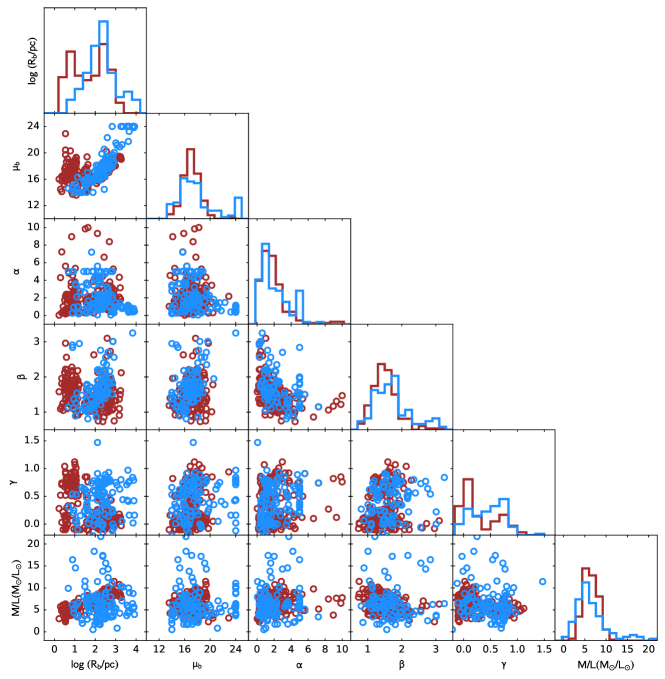
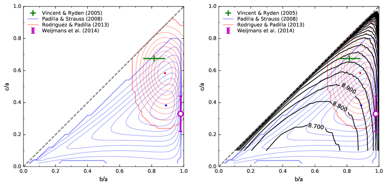
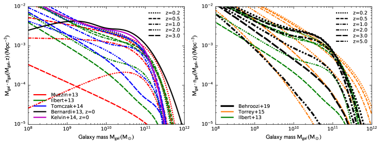
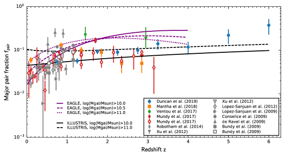
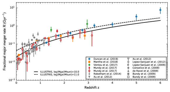
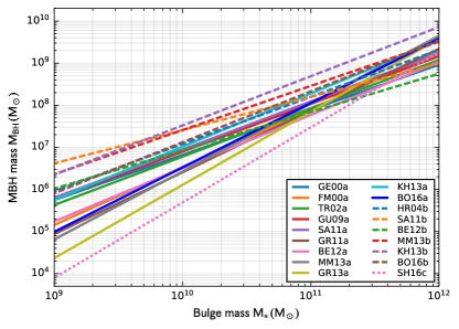
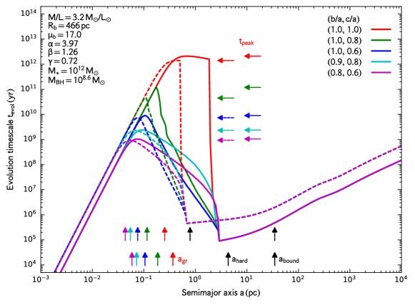
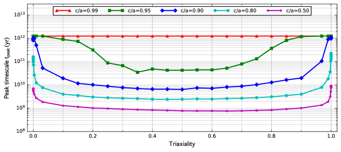

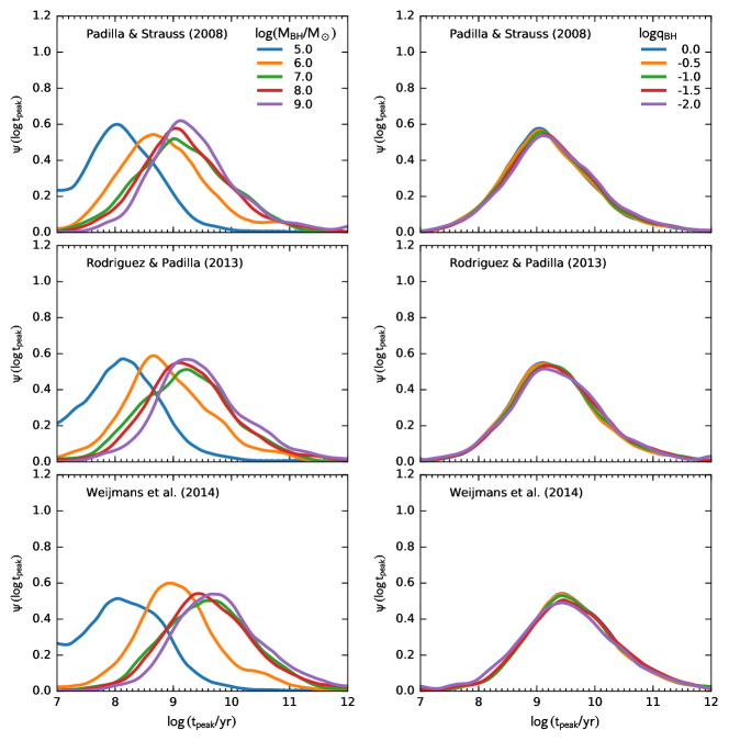
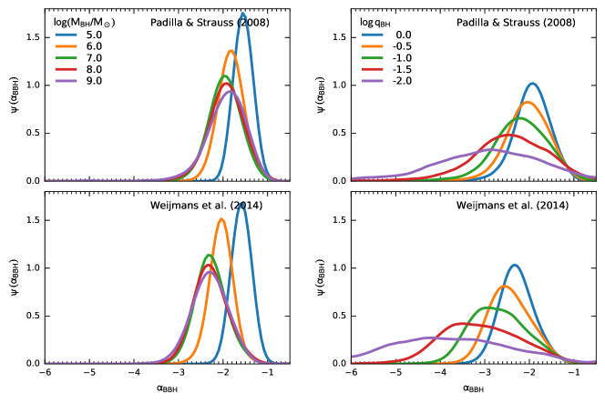
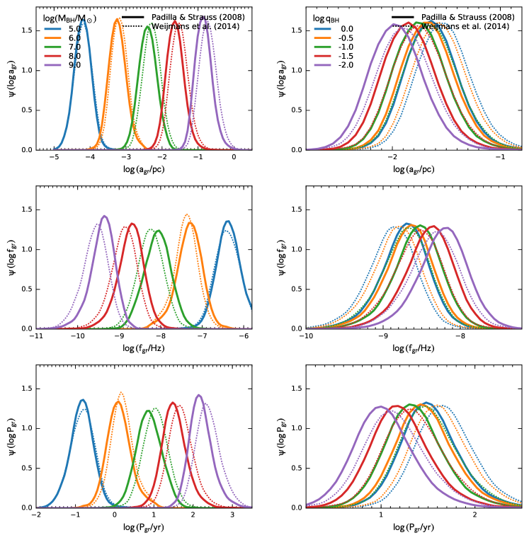
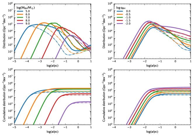
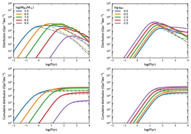
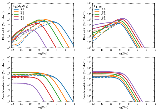
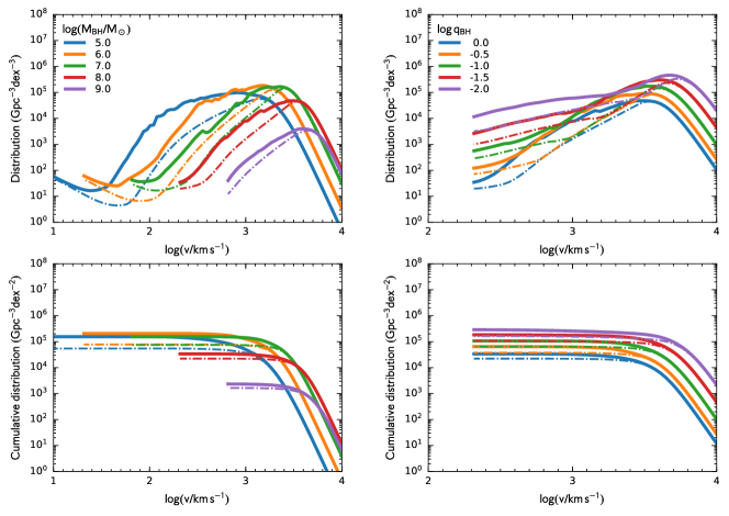
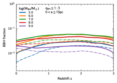
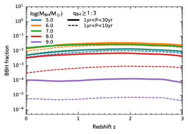
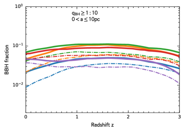

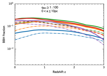
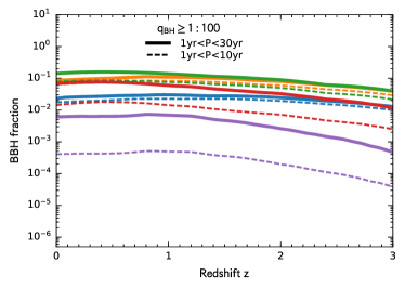
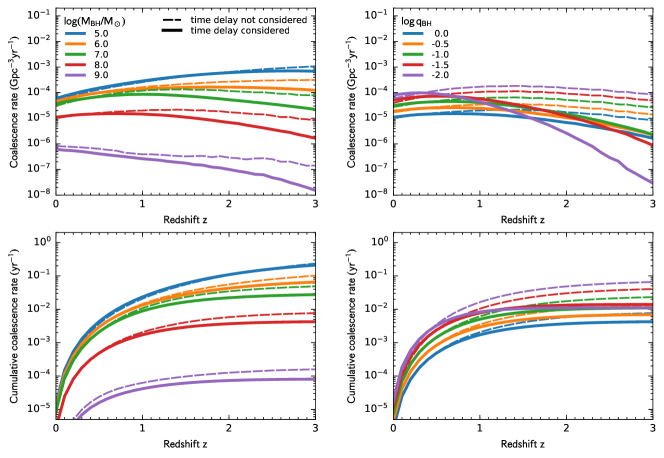
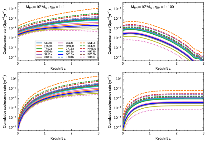
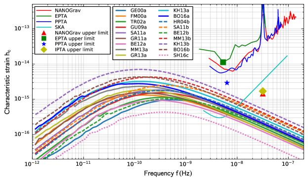
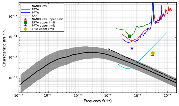
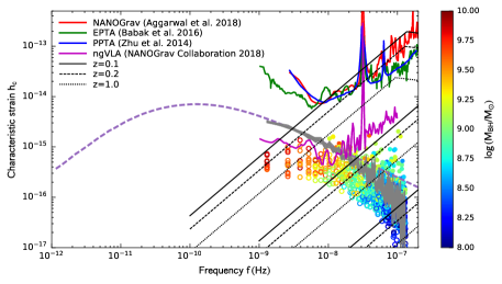
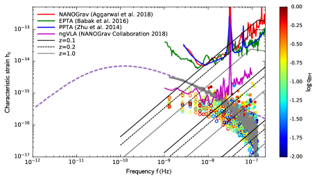


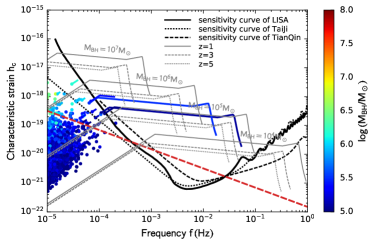

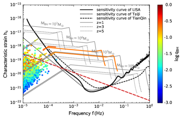
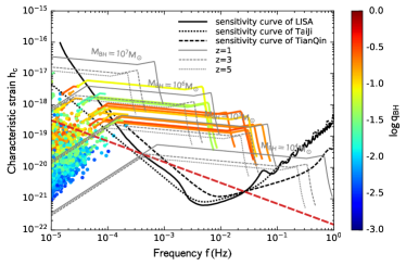
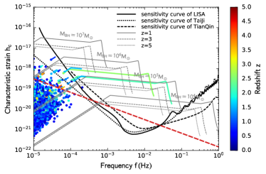
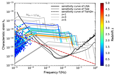
| Abbr | Drop | Reference | |||||||||
|---|---|---|---|---|---|---|---|---|---|---|---|
| dex | |||||||||||
| GE00a | – | 3.75 | 8.08 | 0.30 | -15.69 | -15.80 | 0.11 | -9.28 | 3.27 | 0.27 | Gebhardt et al. (2000) |
| FM00a | – | 4.80 | 8.14 | 0.30 | -15.71 | -15.85 | 0.14 | -9.87 | 4.57 | 0.12 | Ferrarese & Merritt (2000) |
| TR02a | – | 4.02 | 8.13 | 0.30 | -15.67 | -15.79 | 0.12 | -9.48 | 3.65 | 0.20 | Tremaine et al. (2002) |
| GU09a | – | 3.96 | 8.23 | 0.31 | -15.58 | -15.70 | 0.13 | -9.54 | 3.63 | 0.21 | Gültekin et al. (2009) |
| SA11a | – | 4.00 | 8.29 | 0.33 | -15.52 | -15.65 | 0.13 | -9.60 | 3.78 | 0.19 | Sani et al. (2011) |
| GR11a | – | 5.13 | 8.13 | 0.34 | -15.71 | -15.85 | 0.14 | -9.84 | 3.94 | 0.17 | Graham et al. (2011) |
| BE12a | – | 4.42 | 7.99 | 0.36 | -15.79 | -15.91 | 0.12 | -9.61 | 4.18 | 0.15 | Beifiori et al. (2012) |
| MM13a | – | 5.64 | 8.32 | 0.38 | -15.56 | -15.73 | 0.17 | -9.93 | 3.96 | 0.17 | McConnell & Ma (2013) |
| GR13a | – | 6.08 | 8.15 | 0.41 | -15.68 | -15.86 | 0.18 | -9.84 | 3.38 | 0.25 | Graham & Scott (2013) |
| KH13a | – | 4.42 | 8.50 | 0.29 | -15.40 | -15.55 | 0.15 | -9.90 | 4.25 | 0.15 | Kormendy & Ho (2013) |
| BO16a | – | 5.35 | 8.32 | 0.49 | -15.51 | -15.69 | 0.18 | -9.98 | 3.99 | 0.17 | van den Bosch (2016) |
| HR04b | 1.12 | – | 8.20 | 0.30 | -15.50 | -15.62 | 0.12 | -9.50 | 3.72 | 0.20 | Häring & Rix (2004) |
| SA11b | 0.79 | – | 8.20 | 0.37 | -15.30 | -15.42 | 0.12 | -9.41 | 3.59 | 0.21 | Sani et al. (2011) |
| BE12b | 0.91 | – | 7.84 | 0.46 | -15.62 | -15.73 | 0.11 | -9.36 | 3.64 | 0.19 | Beifiori et al. (2012) |
| MM13b | 1.05 | – | 8.46 | 0.34 | -15.24 | -15.38 | 0.14 | -9.72 | 3.74 | 0.20 | McConnell & Ma (2013) |
| KH13b | 1.17 | – | 8.69 | 0.29 | -15.11 | -15.28 | 0.17 | -9.94 | 3.70 | 0.19 | Kormendy & Ho (2013) |
| BO16b | 1.21 | – | 8.33 | 0.49 | -15.31 | -15.47 | 0.16 | -9.89 | 3.74 | 0.19 | van den Bosch (2016) |
| SH16c | 0.50 | 4.50 | 7.70 | 0.25 | -16.09 | -16.22 | 0.14 | -9.48 | 3.38 | 0.24 | Shankar et al. (2016) |
Note. — The BH–host galaxy relations in different works and the characteristic strain amplitudes of the stochastic GWBs obtained with the relations. The BH–host galaxy relations are described by the parameters , , (see Eq. 46), and the intrinsic scatter of the relation (see Section 4.4), and the references to the relations are listed in the last column of the table. Regarding the relation in Ferrarese & Merritt (2000) (FM00a), an intrinsic scatter is not provided in the original work; and here a scatter of is assumed, as listed in the table. The and represent the strain amplitudes at , obtained with and without including the time delays between galaxy mergers and BBH coalescences in our model, respectively. The column of “Drop” gives the values of . The parameter is the turnover frequency of the obtained GWB spectrum, is the power describing the spectrum at the low-frequency end of the spectrum, and is a parameter to describe the shape transition of the GWB spectrum around the turnover frequency (see Eqs. 53 and 54). The numbers in bold are about the medians of and , respectively.