subsecref subsecname = thmref thmname = theorem  lemref lemname = lemma 

Inference, prediction and optimization of non-pharmaceutical interventions using compartment models: the PyRoss library

PyRoss is an open-source Python library that offers an integrated platform for inference, prediction and optimisation of non-pharmaceutical interventions in age- and contact-structured epidemiological compartment models. This report outlines the rationale and functionality of the PyRoss library, with various illustrations and examples focusing on well-mixed, age-structured populations. The PyRoss library supports arbitrary age-structured compartment models formulated stochastically (in terms of master equations) or deterministically (as systems of differential equations) and allows mid-run transitioning from one to the other. By supporting additional compartmental subdivision ad libitum, PyRoss can emulate time-since-infection models and allows medical stages such as hospitalization or quarantine to be modelled and forecast. The PyRoss library enables fitting to epidemiological data, as available, using Bayesian parameter inference, so that competing models can be weighed by their evidence. PyRoss allows fully Bayesian forecasts of the impact of idealized non-pharmaceutical interventions (NPIs) by convolving uncertainties arising from epidemiological data, model choice, parameters, and intrinsic stochasticity. Algorithms to optimize time-dependent NPI scenarios against user-defined cost functions are included. PyRoss’s current age-structured compartment framework for well-mixed populations will in future reports be extended to include compartments structured by location, occupation, use of travel networks and other attributes relevant to assessing disease spread and the impact of NPIs. We argue that such compartment models, by allowing social data of arbitrary granularity to be combined with Bayesian parameter estimation for poorly-known disease variables, could enable more powerful and robust prediction than other approaches to detailed epidemic modelling. We invite others to use the PyRoss library for research to address today’s COVID-19 crisis, and to plan for future pandemics.

Chapter 0 Introduction

This report introduces PyRoss, a Python library for inference, forecasting and optimisation of non-pharmaceutical interventions (NPIs), using compartment models of epidemics. These models are very widely used in epidemiology [1, 2, 3], including simple examples such as SIR, but also more complicated variants [4, 5, 6, 7], some of which are discussed further below. The central modelling philosophy is to group individuals into compartments, which correspond to disease states (such as susceptible / infectious) and may be further divided by age, and by objective medical states (for example, seropositive, hospitalized, in ICU, on ventilator). This leads to a broad class of models that are intermediate in detail between simple compartment models (such as SIR [1]) and agent-based or similar models where the population is disaggregated into synthetic individuals [8].

The functionality of PyRoss not only includes simulation of such compartment models, but also automates inference of their parameters from data, and construction of Bayesian forecasts. In addition, it offers framework for modelling NPIs, and optimisation of their parameters (for example, the length of a lockdown) against user-defined cost functions. While the simulation aspects of PyRoss may be comparable to those available elsewhere (such as epiModel [9]), its integration of inference and optimisation engines create enhanced functionality within a unified and relatively transparent open-source coding environment.

1 Rationale for compartment models

PyRoss is built around Markovian compartment models, in which a system’s future evolution depends only on the current occupancies of the compartments. This leads to several useful simplifications – the average dynamics of a large population can be obtained by solving a system of ordinary differential equations, and the stochastic dynamics of a finite population can be simulated by a simple (Markovian) stochastic process. On the other hand, such models are sometimes criticised [2] because they result in exponential distributions of residence times in each compartment, which is often inconsistent with realistic disease progression. To address this, time-since-infection (TSI) models may be used [10, 11, 12, 13, 14, 15, 2].

Nevertheless, the behaviour of TSI models can be captured by compartment models, at the modest cost of introducing additional compartments. This is called the method of stages [4, 5, 6, 7]. In stochastic modelling, it amounts to replacing a non-Markovian model by a Markovian one on a larger space (which here is a model with extra compartments). PyRoss supports an unlimited number of compartments, which achieves high generality while retaining the conceptual and computational advantages of compartment models. Subdivision of a compartment into $k$ stages, even for modest values such as $k=5,$ already allow considerable flexibility in capturing non-Markovian distributions of residence times within different disease states. Larger values of $k$ can of course be used, if required.

Lifting any restriction on the number of compartments has advantages beyond the TSI issue just described. For example, the medical data used to infer parameters is often provided in the form of compartment populations, such as ICU occupancy or serological test data (perhaps segregated by age). The observed population of these added compartments can then inform the parameters of the model, improving predictions of the future prevalence of these (and other) outcomes. This is valuable when, as with COVID-19, avoiding saturation of ICU or ventilator provision is a policy objective.

One standard use of compartment models is to address age-structured populations. Crucially, this resolves the assortative character of social contacts through which disease transmission occurs. By compartmenting into age bands, representing the contact rates between each pair of bands in terms of a contact matrix, and partitioning this matrix further into home- based, school-based, workplace-based and ‘other’ components (on which NPIs have separately estimable effects) one can, within a well-mixed population model, prediction epidemic evolution and NPIs outcomes in countries with different demographic and societal structures. Indeed the first use of PyRoss was to make such predictions for COVID-19 in India [16] where three-generation households are widespread. More generally, resolving the age structure of an epidemic is clearly essential in modelling diseases whose transmission and/or morbidity shows a strong age-dependence.

2 NPIs and compartment structure

NPIs are modelled in PyRoss using either user-specified or inference-based modifications to the contact matrices. For instance the closure of schools reduces the matrix elements between school-going age groups by the school-based contact contribution. It is clear in this context that subdivision to resolve the contact matrix more finely (for instance, splitting work environments by occupation or sector, and adding retail, catering and entertainment contributions) would improve predictive power. Such models could address the fact that NPIs such as social distancing will have different efficacies (and also different costs, see below) in each context. Although PyRoss currently implements only home, school and work compartments, finer subdivision requires no fundamental change to its structure.

A further extension of PyRoss adds a compartment-based treatment of spatial structure whereby locally well-mixed populations in different neighbourhoods exchange individuals by means of additional, reversibly populated compartments describing a “commuterverse”. The resulting codebase, PyRossGeo , which has been implemented for a model of Greater London, will be the subject of a separate report. As described there, this approach to spatial modelling could offer advantages over agent-based and other approaches, particularly in mid-epidemic where disease dynamics may become effectively deterministic even at local scale (at least in a city as densely populated as London).

3 Limitations

Of course, compartment models are not universally applicable. One drawback emerges on considering strong lockdown scenarios in which transmission between households becomes extremely low. This violates the concept of a well-mixed population; disease cannot spread no matter how high the intra-household contact rate. However, it seems plausible that by transferring attention from individuals to households (each described as a set of several individuals that becomes exposed when any one of them is infected) a compartment model for this situation could also be developed. Challenges also arise in modeling track-and-test, quarantine and other individually resolved NPIs, but we suspect some of these challenges can also be overcome by careful compartment design.

We surmise that the full potential of compartment models in epidemic modelling remains unrealized. To help achieve this potential, the PyRoss library currently supports general age-structured compartment models formulated stochastically (in terms of so-called ‘chemical master equations’ or CMEs) or deterministically (as systems of differential equations). The library can automatically switch between stochastic and deterministic descriptions such that the more expensive stochastic sampling is used when compartment numbers are small, as they are in the early and late stages of an epidemic, while the less expensive deterministic sampling is used when compartment numbers are large, as they are near the peak of the epidemic, at least within well-mixed models. This allows for accurate and efficient sampling of entire epidemiological trajectories taking into account the intrinsic stochasticity of the transmission process.

Perhaps the greatest limitation of compartment models is the tendency toward proliferation within such models of large numbers of parameters to describe the transition rates between compartments, many of which cannot be directly measured. A disciplined methodology for parameter estimation is then essential.

4 Bayesian parameter inference and forecasting

Accordingly, PyRoss supports fitting to epidemiological (and other) data using Bayesian parameter inference and model selection. We use the Gauss-Markov limit of the discrete-state continuous-time Markov process described by the relevant chemical master equation for this purpose. Then, the standard machinery of Gaussian process regression can be used to infer parameters. The kernels of the Gaussian process are adapted, via the Gauss-Markov limit, to the models being fitted and these adapted kernels are obtained from the solution of systems of ordinary differential equations. The numerous advantages of Gaussian process regression, in particular tractable inference and the ability to admit latent variables, accrue automatically. The Bayesian model evidence, necessary for model comparison, model selection and model averaging, alongside the Fisher information matrix, necessary for assessing parameter sensitivities, are thereby obtained in PyRoss without the need for computationally expensive sampling methods such as Markov Chain Monte Carlo.

Within PyRoss the future course of an epidemic can be predicted, with Bayesian confidence estimation, from models fitted to data gathered up to the present. These forecasts take into the account uncertainties in data, the epidemiological parameters, choice of models, and the intrinsic stochasticity of the transmission. The Bayesian methodology is known to provide a principled way of managing uncertainty [17, 18], which is inherent in epidemic modelling and prediction.

Bayesian methods also defend against over-fitting, which is a risk in all models with large numbers of parameters. For instance, the CovidSim model of [19] has, we estimate, over 600 parameters, many of which are not readily accounted for even after geographical, social and other data inputs are identified. Over-fitted models, containing parameters unconstrained by data, are liable to be precise but inaccurate forecasters, particularly under data-poor conditions as is currently the case for COVID-19. In contrast, relatively simple compartment models can be adequate forecasters under these same conditions. An appendix to this report gives a tutorial discussion of the Bayesian approach to this topic for the benefit of those unfamiliar with it.

5 Optimising the outcomes of NPIs

NPIs such as lockdown or social distancing each carry a cost (including, but not limited to, economic, medical, social and ethical costs). This can differ substantially between interventions. For measures that treat different age groups differently, age-structured models can be used to assess the their differential impact. Similar remarks apply to other types of compartmenting in more general models, for instance by geographic, social or industrial sector, as we plan to consider in subsequent reports.

By representing NPIs through their effects on contact matrices, PyRoss can provide Bayesian forecasts of the impact of specific interventions (albeit limited in the currently implemented examples to the age-structured case). Intervention strategies that extremise imputed costs can then be found without leaving the platform.

The optimisation methodology provided within PyRoss a principled way of minimising harm in sustained application of NPIs. The exact definition of ‘harm’ is of course controversial and subjective. To create a well posed optimization problem, the first step is formulation of a cost function which encodes mathematically how one type of harm (such as fatalities) is weighed against another (such as unemployment). For obvious reasons, PyRoss leaves the choice of cost function to the user, although a schematic example of the approach is described later in this report.

6 Provenance

PyRoss is named after Sir Ronald Ross, doctor, mathematician and poet. In 1898 he made "the great discovery" in his laboratory in Calcutta "that malaria is conveyed by the bite of a mosquito". Ross won the Nobel Prize for Physiology or Medicine in 1902 and helped lay the foundations of the mathematical modelling of infectious diseases.

As previously mentioned, PyRoss was initially developed to study the age-structured impact of social distancing on the COVID-19 epidemic in India [16]. Currently it is being developed by the authors of this report who form a task team of the RAMP initiative (Rapid Assistance in Modelling the Pandemic) coordinated by the Royal Society. The library can be used directly to study the transmission, and mitigation through NPIs, of infectious diseases for any well mixed demographic where age and social contact structures are available. As described already, extensions to more general compartment models are either nearing completion (PyRossGeo), or readily envisaged within the same coding structure. More will be added as resources allow.

Compartment models in epidemiology have a long history and while a number of references are cited below, we have not had time to survey the literature as thoroughly as we would like in preparing this report. Some parts may therefore cover territory familiar to experts, but our aim here is to present PyRoss to a wider scientific community as an open-source, well coded Python library that combines the flexibility and generality of age-stratified (and prospectively more general) compartment models with appropriate inference and optimization tools. We hope this resource might prove equally valuable to seasoned epidemic modellers and to the many now entering the field for the first time.

7 Remaining chapters

The remainder of this report is structured as follows. In Chapter 2 we provide an overview of metapopulation models of infectious diseases, focussing on age and contact structures. We then sketch a pipeline where models and epidemiological data can be combined, forecasts can be made, and the impact of interventions can be studied in a fully Bayesian manner. In Chapter 3 we outline the theory of inference, prediction, and optimal control of the abstract Markovian epidemic where the pipeline of the preceding chapter can be feasibly realised. In Chapter 4 we provide a bestiary of epidemiological compartment models that illustrate but by no means exhaust PyRoss’s capabilities for model construction. We discuss compartment subdivision to allow non-exponentially distributed infectious periods and also to uncouple combinations of rate parameters that would otherwise not be independent. Although the specific examples we discuss have been hard-optimized for the PyRoss library, we also describe how user-defined models can be implemented with only mildly reduced efficiency while retaining full use of the surrounding inference and optimisation tools. In Chapter 5 we present several fully coded worked examples in PyRoss, touching upon sampling, inference, prediction, control and optimal control. As in the preceding chapter, our purpose is illustrative and focuses on simple rather than fully realistic cases. We conclude in Chapter 6 with a brief summary.

Chapter 1 Inference, Prediction and Optimized Intervention for Compartment Models

Figure 1: Inference, prediction and intervention framework in PyRoss. For explanations of mathematical symbols see Chapter 2.

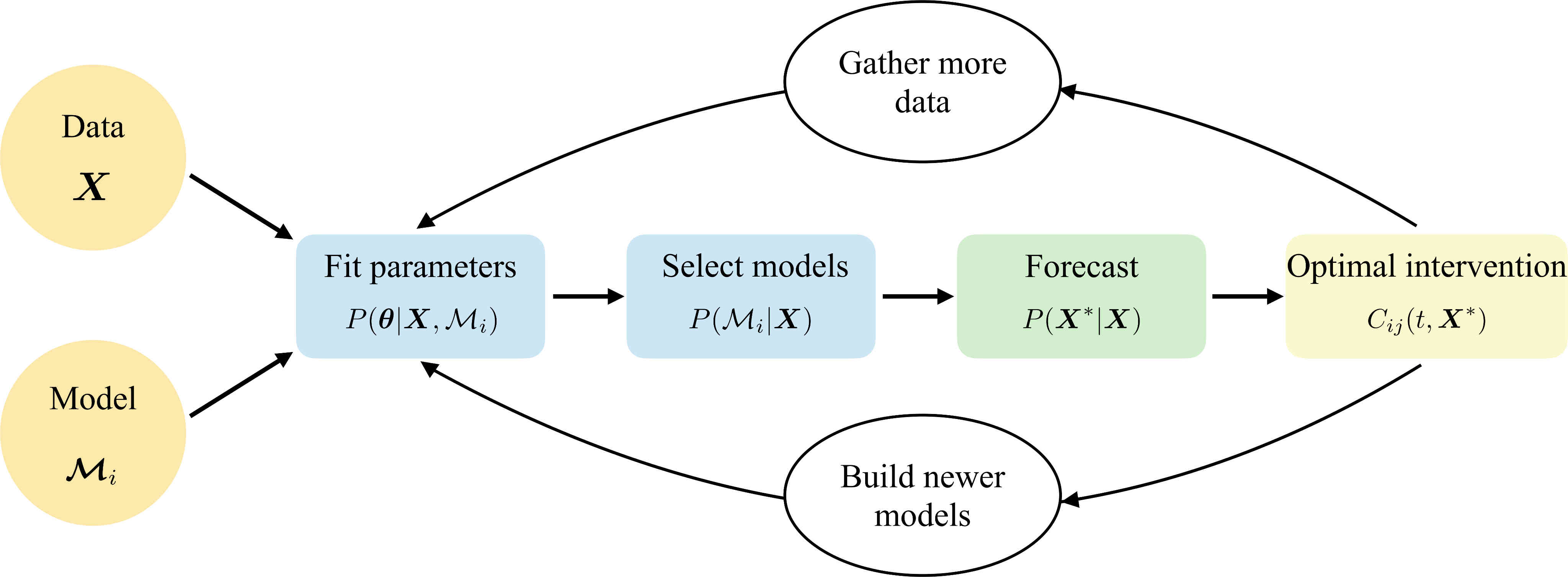
We now specify in more detail the types of model PyRoss currently implements and outline how these form part of an integrated inference, prediction and optimization pipeline, shown schematically in Fig. 1.

1 Compartment models

PyRoss is designed to simulate structured epidemiological compartment models. The basic variable in this class of models is a metapopulation labeled by its epidemiological state (susceptible, infectious, recovered/removed, etc.,) and additional attributes like age, gender, geographic location and so on [1, 2, 20, 21, 22]. These additional attributes define the structure of the model. The user can specify more disease-state compartments than is traditional, and examples described later in this report include not only susceptible ($S$), infectious ($I$), exposed ($E$), quarantined ($Q$) and recovered/removed ($R$) states but also, for example, subdivisions of I into asymptomatic and symptomatic, with the latter further divided into hospitalized and in intensive care. Additionally, the infectious class or classes can be subdivided into $k$ time stages [4, 5, 6, 7] to approximate fixed overall residence times as described in Chapter Inference, prediction and optimization of non-pharmaceutical interventions using compartment models: the PyRoss library. Similar latent compartments can also be used to overcome other constraints on the disease dynamics that arise from a few-compartment approach.

The compartment subdivision scheme exploits PyRoss’s efficient representation of transitions between compartments as Markovian jump processes of given rate. This means that the residence time in any (sub-)compartment is exponentially distributed unless the jump rates themselves vary in time (as they do if an NPI regime is changed). The time evolution of the compartment occupancy variables are accordingly described by chemical master equations with time-dependent rates and, when compartmental fluctuations are small so that deterministic dynamics arises, by ordinary differential equations.

2 Age structure and contact matrices

An infectious disease is spread by social contacts which are typically assortative in age [1, 23]. Therefore, it is important to account for the country-specific age and social contact structures when modelling the spread of infection. Also, in diseases where morbidity and mortality are strongly age-dependent, as with COVID-19, it is important not only to know how many people are likely to be infected but also how they are distributed in age. For example, India is one of the few countries in the world with a high prevalence of three-generation households. This poses a large risk to the elderly, as they are more likely to catch the disease from second- and third-generation members of the household with greater social contacts. PyRoss has already provided the first age-structured forecasts of morbidity and mortality of the COVID-19 epidemic in India [16] and can do so for any community in which the appropriate age stratified contact structure is available, including the 152 countries reported in [24]; see Fig. 1 for examples.

Figure 1: Age and contact structures of the populations of UK (top), Italy and India (bottom). The first column shows population pyramids by age and gender. The second third and fourth columns show the contact structures in households, workplaces and schools respectively. The darker colours represent greater contacts. Taken from [24].

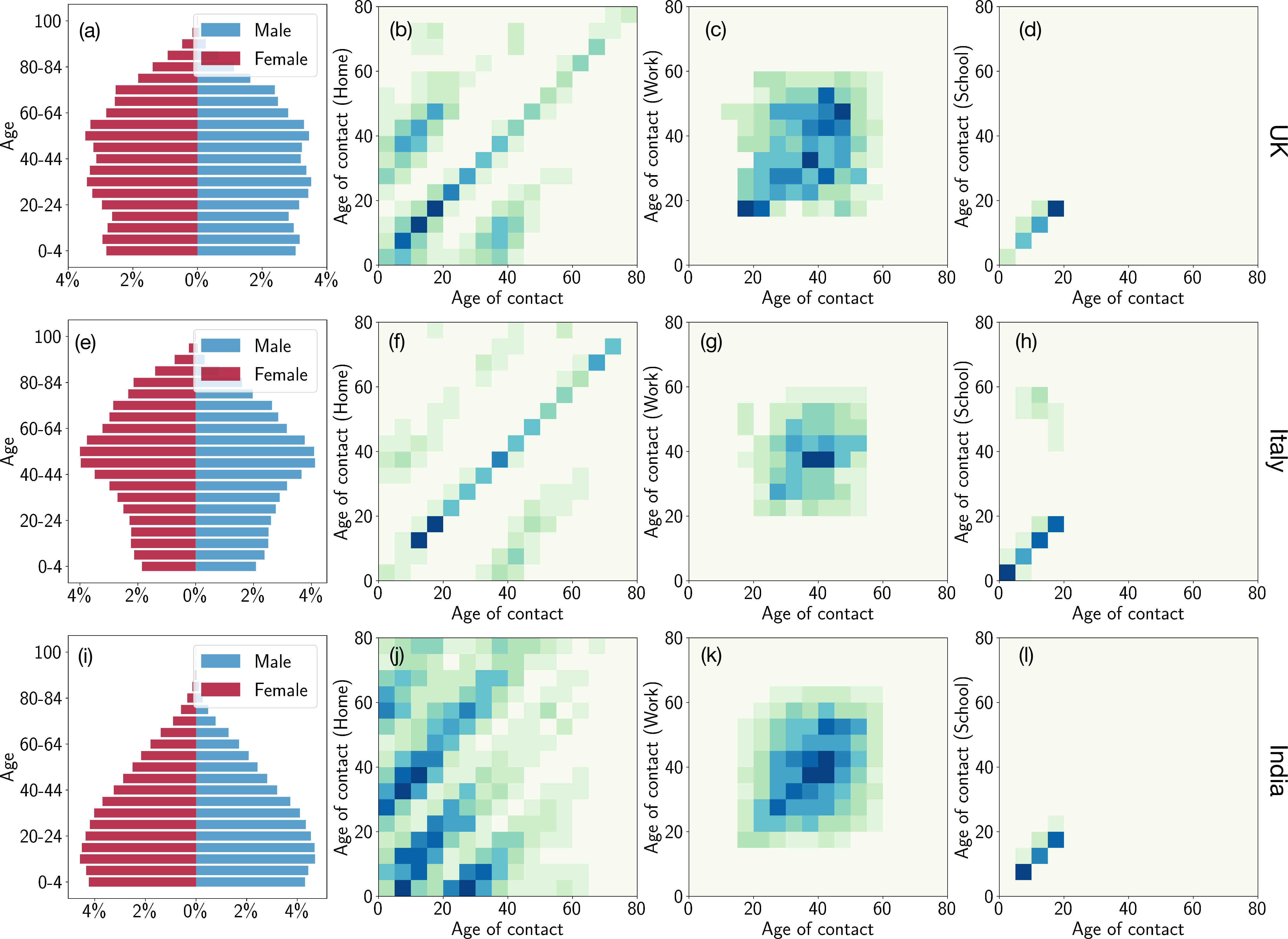
The resulting differences between countries can be substantial. For instance, with a simple SIR model [25, 2, 1, 3], the difference between age and contact structures in UK and India leads to a basic reproduction ratio $\mathcal{R}_{0}$ that is more than 50 percent higher in the latter case; see Table 1. This of course means that identical NPIs could suppress the epidemic in one country and fail completely to do so in another. (For similar reasons it could fail in cities but succeed in the countryside, for example.)

Country	Basic reproductive ratio
UK	$\mathcal{R}_{0}=82\beta$
Italy	$\mathcal{R}_{0}=119\beta$
India	$\mathcal{R}_{0}=136\beta$

Table 1: Country-specific basic reproductive ratio of the age-structured SIR model for fixed probability of infection on contact $\beta$ and recovery rate $\gamma=1/7$.

3 Modelling and optimizing NPIs

The purpose of many NPIs, such as lockdown and social distancing, is to reduce either the frequency of social contacts or the transmission rates at each contact. Absorbing the latter into the former, such NPIs simply alter the contact matrix. Age-structured models can therefore address age-structured NPIs; the examples in this report are limited to such cases, retaining for simplicity the simplest three-way breakdown of contact spaces (Fig. 1). As mentioned in Chapter Inference, prediction and optimization of non-pharmaceutical interventions using compartment models: the PyRoss library, further compartmenting in principle allows resolution of NPIs that affect specific subsets of social contacts, such as closing restaurants or public transport systems, without raising major issues of principle.

An obvious example is schools closure, an NPI for which the schools channel of the contact matrix is set to zero – or perhaps some nonzero multiplier of its normal value to describe partial opening. Another simple case is a phased unlock stratified by age-bands. A model with additional structure, such as workplaces stratified by occupation or sector, should allow the outcome of more nuanced NPIs to be predicted in the same way.

In PyRoss, we partition contacts into spheres of home, workplace, school and all other categories, such that the contact matrix can be written as

$$C_{ij}(t) =a^{H}(t)C_{ij}^{H}+a^{W}(t)C_{ij}^{W}+a^{S}(t)C_{ij}^{S}+a^{O}(t)C_{ij}^{O}.$$ (1)

The social contact matrix $C_{ij}$ denotes the average number of contacts made per day by an individual in class $i$ with an individual in class $j$. Clearly, the total number of contacts between group $i$ to group $j$ must equal the total number of contacts from group $j$ to group $i$, and thus, for populations of fixed size the contact matrices obey the reciprocity relation $N_{i}C_{ij}=N_{j}C_{ji}$ [26, 27], where $N_{i}$ is the population in age-group $i$.

In general, PyRoss expects NPIs to be represented by time-dependent contact matrices. Its inference platform for learning from data is structured accordingly to infer time dependent parameters where appropriate. For example, sufficient age-stratified disease data spanning an initially unlocked and subsequently locked-down state, should allow Bayesian prediction of the effects not just of full unlock but of a partial unlock comprising school closure plus home sequestration of people over 70 (say). There are clearly limitations to this, in that the effect of a completely novel intervention cannot be predicted without prior knowledge of its likely effects on contact matrices. However such priors might be provided by expert judgement. Then, upon actually starting the intervention, incoming data can refine and update model parameters to give increasingly confident prediction of its future effects.

For policy purposes it is obviously desirable to allow objective comparison of alternative NPIs. PyRoss supports user-defined cost functions to allow this. Intervention strategies that extremise the chosen cost function can then be found using optimization tools which are built into PyRoss as detailed in Chapter 2.

Chapter 2 Techniques

In this chapter, we describe age-structured epidemiological compartment models formulated as discrete-state continuous-time Markov processes. We present the chemical master equation (CME) that describes such processes and then provide the diffusion and Gauss-Markov approximations of the process. The Gauss-Markov approximation is used for Bayesian parameter inference and to compute the model evidence. Bayesian posterior predictive distributions are used to provide forecasts given epidemiological data. Such forecasts convolve uncertainties arising from epidemiological data, parameters, models, and intrinsic stochasticity. Non-pharmaceutical interventions (NPI) are imposed by altering the contact structures of the models. Incorporating uncertainties, a Bayesian forecast of the effect of such interventions can be obtained. The protocol of the NPI - defined for instance by points of triggering and its duration - can be optimized by extremizing a supplied cost function. This sequence of inference, prediction and intervention can be applied iteratively with the arrival of newer data, as shown pictorially in Fig.(1), leading to improved epidemiological compartment models.

1 Discrete-state continuous-time Markov process

We consider a structured metapopulation

$$\boldsymbol{n}=(n_{1},\ldots n_{L\times M})$$ (1)

consisting of $L$ classes of epidemiological states and $M$ age-compartments. The $\xi$-th transition between compartments can be written down in its most general form as

$$\xi\text{-th transition step:}\quad\boldsymbol{n}\xrightarrow{w_{\xi}}\boldsymbol{n}+\boldsymbol{r}_{\xi}$$ (2)

where $\boldsymbol{r}_{\xi}$ is the vector of change and $w_{\xi}$ is the rate for the transition $\xi$. This gives the chemical master equation (CME) for the evolution of joint distribution over states $P(\boldsymbol{n},t)$ :

$$\partial_{t}P(\boldsymbol{n},t)=\sum_{\xi}\left[w_{\xi}(t,\boldsymbol{\theta},\boldsymbol{n}-\boldsymbol{r}_{\xi})P(\boldsymbol{n}-\boldsymbol{r}_{\xi},t)-w_{\xi}(t,\boldsymbol{\theta},\boldsymbol{n})P(\boldsymbol{n},t)\right].$$ (3)

Here $\boldsymbol{\theta}=(\theta_{1},\ldots,\theta_{k})$ is the set of parameters for transitions between the states. The CME describes a discrete-state continuous-time Markov process on the positive integers. The CME resists solution for all but the simplest form of the transition rates, which can be at most linear. Since the transmission of contagion necessarily involves the contact of, at least, pairs the rates in epidemiological models cannot be linear. Numerical sampling, or, analytical approximations become necessary to extract model behavior from the CME. We describe the analytical approximations in the next section and numerical sampling in Section (7).

2 Approximations

The family of approximations we consider here replaces the discrete-state continuous-time Markov process by a continuous-time continuous-state Markov process. In this diffusion limit, the transitions $\boldsymbol{n}\xrightarrow{}\boldsymbol{n}+\boldsymbol{r}_{\xi}$ in the discrete state space $\boldsymbol{n}$ are replaced by transitions $\boldsymbol{x}\xrightarrow{}\boldsymbol{x}+d\boldsymbol{r}$, in a continuous state space $\boldsymbol{x}$ with continuous increments $d\boldsymbol{r}$ and appropriately chosen rates. The continuous state $x$ is usually the discrete state rescaled by the size of the population, $\boldsymbol{x}=\boldsymbol{n}/N$. This makes it apparent that the diffusion approximation is appropriate when the population size $N$ is large. Here $N=\sum_{i=1}^{M}N_{i}$ and $N_{i}$ is total population in the age-group $i=1,2,\dots M$.

1 Diffusion limit and the $\Omega$-expansion

Formally, the diffusion limit is obtained by truncating the Kramers-Moyal expansion of the CME to second order. The theorem due to Pawula [28] constrains this truncation to be the only one that yields positive-definite probability distributions. The result is the so-called chemical Fokker-Planck equation (CFPE) with drift and diffusion coefficients that are jump moments of the transition rates of the CME [29, 30]:

$$\partial_{t}P(\boldsymbol{x},t)=L(t\boldsymbol{,\theta,x})P(\boldsymbol{x},t),\quad L=-\frac{\partial}{\partial x_{i}}A_{i}(t,\boldsymbol{\theta},\boldsymbol{x})+\tfrac{1}{2}\frac{\partial^{2}}{\partial x_{i}\partial x_{j}}B_{ij}(t,\boldsymbol{\theta},\boldsymbol{x}),$$ (1)

where

$$\boldsymbol{A}(t,\boldsymbol{\theta},\boldsymbol{x}) =\sum_{\xi}\boldsymbol{r}_{\xi}w_{\xi}(t,\boldsymbol{\theta},\boldsymbol{x}),$$ (2)

$$\boldsymbol{B}(t,\boldsymbol{\theta},\boldsymbol{x}) =\sum_{\xi}\boldsymbol{r}_{\xi}\boldsymbol{r}_{\xi}w_{\xi}(t,\boldsymbol{\theta},\boldsymbol{x}).$$ (3)

The equivalent Itô stochastic differential equation (SDE) is,

$$d\boldsymbol{x}=\boldsymbol{A}(t,\boldsymbol{\theta},\boldsymbol{x})dt+\boldsymbol{\sigma}(t,\boldsymbol{\theta},\boldsymbol{x})\cdot d\boldsymbol{W}$$

where $\boldsymbol{\sigma}$ is such that $\boldsymbol{\sigma}\boldsymbol{\sigma}^{T}=\boldsymbol{B}$ and $\boldsymbol{W}$ is a $L\times M$ dimensional Wiener process with zero mean and unit variance.

The diffusion approximation yields an Ito process with configuration-dependent noise. A further approximation due to Van Kampen decomposes the diffusion process into a mean process without noise and a fluctuation which is described by a time-dependent Ornstein-Uhlenbeck process. The resulting process is both Markovian and Gaussian. In this linear noise approximation (LNA), the state is expressed as,

$$\boldsymbol{x}(t)=\boldsymbol{x}^{0}(t)+\frac{1}{\sqrt{\Omega}}\boldsymbol{x}^{1}(t)$$ (4)

where $\Omega=N$ is the system size. The two components satisfy

$$d\boldsymbol{x}^{0}(t)=\boldsymbol{A}(t,\boldsymbol{\theta},\boldsymbol{x}^{0})dt,$$ (5)

$$d\boldsymbol{x^{1}}=\boldsymbol{J}(t,\boldsymbol{\theta},\boldsymbol{x}^{0})\cdot\boldsymbol{x^{1}}dt+\boldsymbol{\sigma}(t,\boldsymbol{\theta},\boldsymbol{x}^{0})\cdot d\boldsymbol{W},$$ (6)

where

$$J_{ij}(t,\boldsymbol{\theta},\boldsymbol{x}^{0})=\partial_{j}A_{i}(t,\boldsymbol{\theta},\boldsymbol{x})\Big{|}{}_{\boldsymbol{x}=\boldsymbol{x}^{0}}$$

is the time-dependent Jacobian evaluated at $\boldsymbol{x}^{0}(t)$. The lowest order term $\boldsymbol{x}^{0}$ describes the mean evolution whereas the next order term $\boldsymbol{x}^{1}$ characterises the Gaussian fluctuation around the deterministic trajectory. The fluctuation $\boldsymbol{x}^{1}$ is a non-stationary Ornstein Uhlenbeck process whose mean and variance can be obtained for any point on the mean trajectory.

As a note of caution, there are some subtleties associated with whether the high order terms can grow significantly over time. This is particularly relevant to us as the growth is exponential at the early stage of an epidemic, where the approximation is not likely to be good.

2 Deterministic limit

From the $\Omega$-expansion, we obtain the deterministic limit for free as the evolution of the mean $\bar{\boldsymbol{x}}=\boldsymbol{x}^{0}+\expectationvalue{\boldsymbol{x}^{1}}$. It is simple to show that the mean obeys the same equation as $\boldsymbol{x}^{0}$,

$$\frac{d\bar{\boldsymbol{x}}}{dt}=\boldsymbol{A}(t,\boldsymbol{\theta},\boldsymbol{\bar{x}})$$

In pyross.deterministic, the rescaling of $\beta$ is built in to suit simulations with both intensive and extensive variables.

3 Inference

In this section, we describe inference of parameters $\boldsymbol{\theta}=(\theta_{1},\ldots,\theta_{k})$ performed by the pyross.inference module. The data consists of the time series

$$\boldsymbol{X} =\{x_{i}(t_{\nu})\,\,|\,\,i=1,\ldots M\times L;\nu=1,\ldots N_{t}\}$$ (1)

of the values of the components $x_{i}(t_{\nu})$ at the times $t_{\nu}$. The module is capable of inferring the parameters with full and partial information; in the latter case, the latent variables are also inferred. The module determines Bayesian credible intervals for the inferred parameters, which can be supplied to pyross.forecast to perform Bayesian forecasting with both parameter uncertainty and inherent stochasticity. In the future, mode selection will be added to pyross.inference to measure how well the various epidemiological models fit the data.

1 Non-stationary Gauss-Markov process

Consider the time interval $(t_{\nu},t_{\mu}$) with initial condition $\boldsymbol{x}(t_{\nu})=\boldsymbol{x^{\prime}}$. The outcome of the $\Omega$-expansion is a Gauss-Markov process, implying that the conditional probability $P_{1|1}(\boldsymbol{x},t_{\mu}|\boldsymbol{x}^{\prime},t_{\nu})$ follows a Gaussian distribution determined uniquely by its conditional mean $\bar{\boldsymbol{x}}(t_{\mu})=\expectationvalue{\boldsymbol{x}(t_{\mu})|\boldsymbol{x}^{\prime}}$ and conditional variance, denoted as $\boldsymbol{\Sigma}$ [31].

$$\boldsymbol{x},t_{\mu}|\boldsymbol{x}^{\prime},t_{\nu}\>\sim\mathcal{N}(\bar{\boldsymbol{x}}(t_{\mu}),\boldsymbol{\Sigma}(t_{\mu}))$$

Recall from section 2 that the mean obeys the deterministic equation,

$$\frac{d\bar{\boldsymbol{x}}}{dt}=\boldsymbol{A}(t,\boldsymbol{\theta},\boldsymbol{\bar{x}})$$

with the initial condition $\bar{\boldsymbol{x}}(t_{\nu})=\boldsymbol{x}^{\prime}$, which can be solved numerically with pyross.deterministic. The conditional variance, defined as,

$$\boldsymbol{\Sigma}(t)=\expectationvalue{\boldsymbol{x}(t)\boldsymbol{x}^{T}(t)|\boldsymbol{x}^{\prime},t_{\nu}}-\bar{\boldsymbol{x}}(t)\bar{\boldsymbol{x}}(t)^{T}$$

only has contributions from the fluctuating term $\boldsymbol{x}^{1}$ since $\boldsymbol{x}^{0}$ evolves deterministically,

$$\boldsymbol{\Sigma}(t)=\frac{1}{\Omega}\left[\expectationvalue{\boldsymbol{x}^{1}(t)(\boldsymbol{x}^{1})^{T}(t)|0,t_{\nu}}\right]$$

where we note that the mean of $\boldsymbol{x}^{1}$ remains zero as long as we choose $\boldsymbol{x}^{1}(t_{\nu})=0$ (which can always be done as the splitting of the initial condition $\boldsymbol{x}$’ into $\boldsymbol{x}^{0}$ and $\boldsymbol{x}^{1}$ is arbitrary). It is a well established result that the covariance of an Ornstein-Uhlenbeck process evolves according to the time-dependent differential Lyapunov equation [30, 29],

$$\dot{\boldsymbol{\Sigma}}(t)=\boldsymbol{J}(\bar{\boldsymbol{x}}(t),t)\boldsymbol{\Sigma}(t)+\boldsymbol{\Sigma}(t)\boldsymbol{J}^{T}(\bar{\boldsymbol{x}}(t),t)+\boldsymbol{B}(\bar{\boldsymbol{x}}(t),t)/\Omega$$ (2)

For our models of interest, the Lyapunov equation cannot be solved analytically and is computed numerically in pyross.inference. For improved accuracy, $\boldsymbol{J}$ and $\boldsymbol{B}$, both of which are functions of $\bar{\boldsymbol{x}}(t)$, are computed by interpolating the numerical solution of the deterministic equation using Chebyshev polynomials. Once both the mean and the variance are computed, the conditional probability $P_{1|1}(\boldsymbol{x},t_{\nu+1}|\boldsymbol{x}(t_{\nu}),t_{\nu})$ is given by

$$\ln P_{1|1}(\boldsymbol{x},t_{\mu}|\boldsymbol{x}^{\prime},t_{\nu})=-\left(\frac{1}{2}\boldsymbol{\Delta}_{\mu}^{T}\boldsymbol{\Sigma}_{\mu}^{-1}\boldsymbol{\Delta}_{\mu}+\frac{1}{2}\ln\det 2\pi\boldsymbol{\Sigma}_{\mu}\right)$$

where $\Delta_{\mu}=\boldsymbol{x}-\bar{\boldsymbol{x}}(t_{\mu})$ is the deviation of the endpoint $\boldsymbol{x}$ from the deterministic trajectory.

2 Parameter inference

The conditional probability can be computed as above for each time step, the posterior, using flat priors enforcing positive parameters, is given as the sum of the conditional probabilities,

$$\ln P(\boldsymbol{\theta}|\boldsymbol{X})=-\sum_{\mu=1}^{N_{t}}\left(\frac{1}{2}\boldsymbol{\Delta}_{\mu}^{T}\boldsymbol{\Sigma}_{\mu}^{-1}\boldsymbol{\Delta}_{\mu}+\frac{1}{2}\ln\det 2\pi\boldsymbol{\Sigma}_{\mu}\right).$$ (3)

Here $\boldsymbol{\Delta}_{\mu}=\boldsymbol{x}(t_{\mu})-\bar{\boldsymbol{x}}(t_{\mu})$. This is then used to numerically obtain the MAP estimates for the parameters. Near the onset of an epidemic, the higher order fluctuations can grow exponentially and significantly deviate from the mean trajectory, to resolve this issue, one needs to sample more frequently where the growth rate (effectively $R_{0}$) is large.

3 Latent variables

With limited information, we may only be able to observe a few components $\boldsymbol{X}_{\mathrm{Reduced}}=\{x_{i}(t_{\nu})\,\,|\,\,i=1,...M_{\mathrm{Reduced}}\times L_{\mathrm{Reduced}};\nu=1,\ldots N_{t}\}$, e.g. the number of confirmed cases and deaths.

The first step towards inference for latent variables is to express the probability of an full time series for a given set of parameters. One would then need to trace out unobserved degrees of freedom. However, this is hard to do in practice, because the joint distribution may be highly non-Gaussian. This is the case even though the propagator itself is Gaussian, because $\boldsymbol{\varSigma}$ and $\bar{\boldsymbol{x}}$ may depend on $\boldsymbol{x}$. Nonetheless, Gaussian inference is possible for latent variables if the system-size expansion remains approximately valid for time intervals as long as the whole observed time series. Then, all typical trajectories remain close to the mean of the time series, evolving according to the ODE

$$\partial_{t}\boldsymbol{\bar{\boldsymbol{x}}}=\boldsymbol{A}(\bar{\boldsymbol{x}}),$$ (4)

with the drift vector $\boldsymbol{A}$. One has to be careful, though, because the Jacobian of $\boldsymbol{A}$ typically has positive eigenvalues which results in exponential growth of any deviation from the mean. We need a sufficiently large system size $N$.

We now write $\boldsymbol{x}(t)=\bar{\boldsymbol{x}}(t)+\boldsymbol{\Delta}(t)$. The variable $\boldsymbol{\Delta}=\boldsymbol{x}^{1}/\sqrt{\Omega}$ and therefore also evolves according to an Ornstein Uhlenbeck process. The conditional probability distribution for $\boldsymbol{\Delta}$ at time $t_{\mu}$ given its value at time $t_{\nu}$ is

$$\boldsymbol{\Delta}_{\mu},t_{\mu}|\boldsymbol{\Delta}_{\nu},t_{\nu}\sim\mathcal{N}(\boldsymbol{U}_{\mu}\boldsymbol{\Delta}_{\nu},\boldsymbol{\Sigma}_{\mu})$$ (5)

where the matrix $\boldsymbol{U}_{\mu}=\boldsymbol{U}(t_{\mu})$ is the time evolution operator, defined by the equation $\partial_{t}\boldsymbol{U}(t)=\boldsymbol{J}(\bar{\boldsymbol{x}}(t))\boldsymbol{U}(t)$. It yields the mean of $\boldsymbol{\Delta}(t_{\mu})$ for given $\boldsymbol{\Delta}(t_{\nu})$. $\boldsymbol{\Sigma}_{\mu}$ is calculated from Eq.2, but $\bar{x}$ is different, since we couldn’t update it with a recent initial condition. For a Gaussian initial distribution with covariance $\boldsymbol{\Sigma}_{0}$, the conditional probabilities are concatenated to yield the joint distribution. The overall covariance matrix for the vectors $(\boldsymbol{\Delta}(t_{1}),\ldots,\boldsymbol{\Delta}(t_{N_{t}}))^{T}$ is given by the inverse of the following tridiagonal block matrix:

$$\boldsymbol{\varSigma}^{-1}=\left(\begin{matrix}\\ \boldsymbol{\Sigma}_{1}^{-1}+\boldsymbol{U}_{2}^{T}\boldsymbol{\Sigma}_{2}^{-1}\boldsymbol{U}_{2}&-{\normalcolor\boldsymbol{U}}_{2}^{T}\boldsymbol{\Sigma}_{2}^{-1}&0&\dots\\ \\ -\boldsymbol{\Sigma}_{2}^{-1}\boldsymbol{U}_{2}&\boldsymbol{\Sigma}_{2}^{-1}+\boldsymbol{U}_{3}^{T}\boldsymbol{\Sigma}_{3}^{-1}\boldsymbol{U}_{3}&-\boldsymbol{U}_{2}^{T}\boldsymbol{\Sigma}_{2}^{-1}&0&\dots\\ \\ 0&-\boldsymbol{\Sigma}_{3}^{-1}\boldsymbol{U}_{3}&\ddots&\ddots\\ \\ \vdots&0&\ddots&\ddots\end{matrix}\right).$$ (6)

Note that after the inversion $\boldsymbol{\varSigma}$ typically has nonzero entries everywhere. With latent observable, we simply eliminate all rows and columns associated with (sub-)indices other than those known. The joint distribution of the remaining then follows as a multivariate Gaussian with the reduced covariance and the mean for the observed variables. In the pyross.inference module, the initial conditions for $\boldsymbol{x}$ are also treated as parameters to be inferred, as they are unknown for the unobserved variables.

4 Model evidence

Bayesian credible intervals (BCI), or standard deviation of the maximum a posteriori (MAP) estimates, can be understood by writing $\boldsymbol{H}=-\boldsymbol{\nabla\nabla}\ln P(\boldsymbol{\theta}|\boldsymbol{X},\mathcal{M}_{i})|_{\boldsymbol{\theta}^{*}}$ for the Hessian, and Taylor expanding the log posterior of the parameters $\boldsymbol{\theta}$, given the data $\boldsymbol{X}$ and the model $\mathcal{M}_{i}$ with $\Delta\boldsymbol{\theta}=\boldsymbol{\theta}-\boldsymbol{\theta}^{*}$, where $\boldsymbol{\theta}^{*}$ are the MAPs [17, 32],

$$P(\boldsymbol{\theta}|\boldsymbol{X},\mathcal{M}_{i})\approx P(\boldsymbol{\theta}^{*}|\boldsymbol{X},\mathcal{M}_{i})\exp\left(-\frac{1}{2}\Delta\boldsymbol{\theta}^{T}\boldsymbol{H}\Delta\boldsymbol{\theta}\right).$$ (7)

This is a local Gaussian approximation to the posterior around its mode with covariance matrix $\boldsymbol{H}^{-1}$. The square root of the diagonal elements of this covariance matrix gives the BCIs.

In case the functional form of the posterior distribution is known, numerical errors associated with finite differences methods can be circumvent by using automatic differentiation (eg ’autograd [33]’). This allows for exact and rapid computation of the Hessian matrix, neither over- nor underestimating the uncertainty of our estimates.

Mostly branded ’the second level of inference’ after the first level of obtaining the MAP estimates, the arguably most important feature of Bayesian inference is model selection. The posterior probability for each model is by Bayes’ theorem

$$P(\mathcal{M}_{i}|\boldsymbol{X})\propto P(\boldsymbol{X}|\mathcal{M}_{i})P(\mathcal{M}_{i}).$$ (8)

In the following we assume a flat model prior $P(M_{i})$, ie we a priori have no reason to prefer one model over an other. This leaves us with the model evidence $P(\boldsymbol{X}|M_{i})$, which at the same time is the normalization constant in Bayes’ theorem for the posterior of the parameters $\boldsymbol{\theta}$ given the data

$$P(\boldsymbol{\theta}|\boldsymbol{X},\mathcal{M}_{i})=\frac{P(\boldsymbol{X}|\boldsymbol{\theta},\mathcal{M}_{i})P(\boldsymbol{\theta}|\mathcal{M}_{i})}{P(\boldsymbol{X}|\mathcal{M}_{i})}.$$ (9)

In order to evaluate the evidence, we have to marginalize the likelihood function over the often high-dimensional parameter space

$$P(\boldsymbol{X}|\mathcal{M}_{i})=\int P(\boldsymbol{X}|\boldsymbol{\theta},\mathcal{M}_{i})P(\boldsymbol{\theta}|\mathcal{M}_{i})d\boldsymbol{\theta}.$$ (10)

However, if the posterior in (LABEL:ParamPost) is reasonably well approximated by a Gaussian, which is expected to be increasingly accurate the more data we use, we can use Laplace’s method to approximate the evidence by

$$P(\boldsymbol{X}|\mathcal{M}_{i})\approx\underbrace{P(\boldsymbol{X}|\boldsymbol{\theta}^{*},\mathcal{M}_{i})}_{Best\,fit\,likelihood}\underbrace{P(\boldsymbol{\theta}^{*}|\mathcal{M}_{i})(2\pi)^{k/2}\det\{\boldsymbol{H}\}^{-1/2}}_{Occam\,factor},$$ (11)

the height of the peak of the integrand in (LABEL:Evd) times its width. The Occam factor automatically penalizes over-fitting [17]. By comparing the contributions of best fit likelihood and Occam factor one can at least qualitatively decide whether this approximation is expected to be sufficient. The evaluation is of course orders of magnitude faster than computing the integral in (LABEL:Evd).

5 Nested sampling

Nested sampling (eg via ’nestle’ package [34]) is an algorithm invented by John Skilling [35], dealing with those high-dimensional integrals in the evidence calculation (LABEL:Evd) by reducing them to one-dimensional integrals over unit range. We have found this to be rather slow for most of our models, but since the evidence has to be calculated only once per model, it might still be feasible to use nested sampling. Especially, when not enough data is available and the Gaussian approximation (LABEL:Gevd) fails to be sufficient, this should be used. The method is slow when running on a single core for the inference on the manifold as described in sec 3. However, we have found that for the tangent space inference described in section 4, nestle is actually reasonably fas. This is simply because of the much faster log-posterior evaluations. With parallel processing of the nested sampling, log-posterior evaluation takes few seconds on a 8 core machine for $M=2$ and $N=5\times 10^{4}$.

4 Tangent space inference

As mentioned before, a self-consistent method of taking the diffusion limit of equation (LABEL:Master) is van Kampen’s system size expansion [30]. With the population densities $\boldsymbol{x}\equiv\boldsymbol{n}/\Omega$, where $\Omega$ is the system size - the total population size, the a posteriori justified ansatz of the $\Omega$-expansion is where $\boldsymbol{x}_{\nu}=\boldsymbol{x}(t_{\nu})$. The mean in 4 evolves according to the macroscopic rate equations (MRE)

$$\dot{\bar{\boldsymbol{x}}}_{\nu}=\boldsymbol{A}(t_{\nu},\bar{\boldsymbol{x}}_{\nu},\boldsymbol{\theta}),$$ (1)

and can thus be found by solving this system of ODEs. The CFPE is equivalent to the Ito stochastic differential equation describing the dynamics of $\boldsymbol{u}$, the so called chemical Langevin equation (CLE),

$$d\boldsymbol{u}_{\nu}=\boldsymbol{J}(t_{\nu},\bar{\boldsymbol{x}}_{\nu},\boldsymbol{\theta})\cdot\boldsymbol{u}_{\nu}dt+\boldsymbol{\sigma}(t_{\nu},\bar{\boldsymbol{x}}_{\nu},\boldsymbol{\theta})\cdot d\boldsymbol{W},\quad\boldsymbol{\sigma}\boldsymbol{\sigma}^{T}=\boldsymbol{B}(t_{\nu},\bar{\boldsymbol{x}}_{\nu},\boldsymbol{\theta}),$$ (2)

with $J_{ab}=\partial_{b}A_{a}$, and $\boldsymbol{W}$ being a multi-dimensional Wiener process. Thus, in this approximation the population density evolves according to the stochastic process

$$d\boldsymbol{x}_{\nu}=\boldsymbol{A}(t_{\nu},\bar{\boldsymbol{x}}_{\nu},\boldsymbol{\theta})dt+\Omega^{-\frac{1}{2}}d\boldsymbol{u}_{\nu},$$ (3)

driven by a small (suppressed by a factor of $\Omega^{-\frac{1}{2}}$) Ornstein-Uhlenbeck noise. Formally re-writing equation (LABEL:SDE) we get

$$\dot{\boldsymbol{x}}_{\nu} =\dot{\bar{\boldsymbol{x}}}_{\nu}+\Omega^{-\frac{1}{2}}\dot{\boldsymbol{u}}_{\nu}$$

$$=\boldsymbol{A}(t_{\nu},\bar{\boldsymbol{x}}_{\nu},\boldsymbol{\theta})+\Omega^{-\frac{1}{2}}\left(\boldsymbol{J}(t_{\nu},\bar{\boldsymbol{x}}_{\nu},\boldsymbol{\theta})\cdot\boldsymbol{u}_{\nu}+\boldsymbol{\epsilon}_{\nu}\right)$$

$$=\boldsymbol{A}(t_{\nu},\bar{\boldsymbol{x}}_{\nu},\boldsymbol{\theta})+\boldsymbol{J}(t_{\nu},\bar{\boldsymbol{x}}_{\nu},\boldsymbol{\theta})\cdot\left(\boldsymbol{x}_{\nu}-\bar{\boldsymbol{x}}_{\nu}\right)+\boldsymbol{\eta}_{\nu},$$ (4)

with the Gaussian white noises $\boldsymbol{\epsilon}_{\nu}\sim\mathcal{N}\left(\boldsymbol{0},\boldsymbol{B}(t_{\nu},\bar{\boldsymbol{x}}_{\nu},\boldsymbol{\theta})\right)$ and $\boldsymbol{\eta}_{\nu}\sim\mathcal{N}\left(\boldsymbol{0},\frac{1}{\Omega}\boldsymbol{B}(t_{\nu},\bar{\boldsymbol{x}}_{\nu},\boldsymbol{\theta})\right)$. Thus, with the change of measure

$$P(\dot{\boldsymbol{x}}_{\nu})d\dot{\boldsymbol{x}}=P(\boldsymbol{\eta}_{\nu})d\boldsymbol{\eta}_{\nu}$$ (5)

and the Jacobian $\partial\eta_{\nu}^{i}/\partial x_{\nu}^{j}=\delta^{ij}$ we obtain a multivariate normal distribution for the likelihood of $\dot{\boldsymbol{x}}$, given the parameters $\boldsymbol{\theta}$

$$P(\dot{\boldsymbol{x}}|\boldsymbol{\theta})=\prod_{\nu=1}^{T}\mathcal{N}\left(\langle\dot{\boldsymbol{x}}_{\nu}\rangle,\frac{1}{\Omega}\boldsymbol{B}(t_{\nu},\bar{\boldsymbol{x}}_{\nu},\boldsymbol{\theta})\right),$$ (6)

with the mean velocity defined by

$$\langle\dot{\boldsymbol{x}}_{\nu}\rangle\equiv\boldsymbol{A}(t_{\nu},\bar{\boldsymbol{x}}_{\nu},\boldsymbol{\theta})+\boldsymbol{J}(t_{\nu},\bar{\boldsymbol{x}}_{\nu},\boldsymbol{\theta})\cdot\left(\boldsymbol{x}_{\nu}-\bar{\boldsymbol{x}}_{\nu}\right).$$ (7)

Assuming improper informative priors, i.e,, flat priors enforcing positive parameters, the log-posterior distribution is

$$\ln P(\boldsymbol{\theta}|\dot{\boldsymbol{x}})=-\sum_{\nu=1}^{T}\left[\frac{\Omega}{2}\left(\dot{\boldsymbol{x}}_{\nu}-\langle\dot{\boldsymbol{x}}_{\nu}\rangle\right)^{T}\cdot\boldsymbol{B}^{-1}\cdot\left(\dot{\boldsymbol{x}}_{\nu}-\langle\dot{\boldsymbol{x}}_{\nu}\rangle\right)+\frac{1}{2}\ln\det\frac{2\pi}{\Omega}\boldsymbol{B}\right].$$ (8)

This posterior distribution, albeit complicated, is analytical up to integration of equation (LABEL:MRE) and thus, can be easily traced by automatic differentiation.

Having obtained the maximum a posteriori (MAP) estimates $\boldsymbol{\theta}^{*}$ one can therefore easily obtain the Hessian $\boldsymbol{H}\equiv-\boldsymbol{\nabla\nabla}\ln P(\boldsymbol{\theta}|\dot{\boldsymbol{x}})|_{\boldsymbol{\theta}^{*}}$ of the posterior distribution and thus, calculate the Laplacian approximation to the evidence for the model $\mathcal{M}_{i}$ [17]

$$P(\dot{\boldsymbol{x}}|\mathcal{M}_{i})\approx\underbrace{P(\dot{\boldsymbol{x}}|\boldsymbol{\theta}^{*},\mathcal{M}_{i})}_{Best\,fit\,likelihood}\underbrace{P(\boldsymbol{\theta}^{*}|\mathcal{M}_{i})(2\pi)^{k/2}\det{}^{-\frac{1}{2}}\boldsymbol{H}}_{Occam\,factor},$$ (9)

and most importantly the Bayesian credible intervals, or error bars of the MAP estimates. Not relying on finite differences-methods enables us to quantify the uncertainties of our predictions in a much more reliable manner.

Due to the just-in-time (JIT) compilation of ‘JAX’ [36], a python machine learning library, it is even possible to compute the multi-dimensional integral for the model evidence

$$P(\dot{\boldsymbol{x}}|\mathcal{M}_{i})=\int P(\dot{\boldsymbol{x}}|\boldsymbol{\theta},\mathcal{M}_{i})P(\boldsymbol{\theta}|\mathcal{M}_{i})d\boldsymbol{\theta}$$

exactly within seconds (nestle). With this, we can pursue the task of Bayesian model averaging for epidemiological models.

Operationally , the stochastic population density vector $\boldsymbol{x}$ is given by the data itself. Its derivative $\dot{\boldsymbol{x}}$ is simply obtained by finite differences (jax.numpy.gradient) [36], no fitting is applied. The mean $\bar{\boldsymbol{x}}$ satisfying the MREs (LABEL:MRE) can be found by solving this system of ODEs for a given set of parameters $\boldsymbol{\theta}$ (jax.experimental.ode.odeint), and therefore, is part of the optimization process of finding the MAPs $\boldsymbol{\theta}^{*}$. The coefficients of the system size expansion $\boldsymbol{A},\,\boldsymbol{J}$ and $\boldsymbol{B}$ depend on the mean.

5 Prediction

In the previous section, we described the inference of model parameters $\boldsymbol{\theta}=(\theta_{1},\ldots,\theta_{k})$ given data $\boldsymbol{X}$ in the form of a time series, c.f. equation (1). We now discuss how the results of this inference are used for prediction in the pyross.forecast module. An example where the forecasting module is used is given in section 5.

1 Posterior predictive distributions

Once given data $\boldsymbol{X}$ has been used to infer parameters $\boldsymbol{\theta}$ of a model $\mathcal{M}_{i}$, the probability to make an observation $\boldsymbol{Y}$ is given by

$$P(\boldsymbol{Y}|\boldsymbol{X},\mathcal{M}_{i})=\int P(\boldsymbol{Y}|\boldsymbol{X},\boldsymbol{\theta},\mathcal{M}_{i})P(\boldsymbol{\theta}|\boldsymbol{X},\mathcal{M}_{i})d\boldsymbol{\theta},$$ (1)

where $\boldsymbol{Y}$ is the observation whose probability one wants to predict. The first term in the integral, called model uncertainty, is the probability that, for given data $\boldsymbol{X}$ and parameters $\boldsymbol{\theta}$, one observes $\boldsymbol{Y}$. The second term, called parameter uncertainty, represents the probability of the parameters $\boldsymbol{\theta}$ itself given the data $\boldsymbol{X}$. As indicated in the notation, all three probabilities are conditional on $\mathcal{M}_{i}$. In the present context, $\boldsymbol{X}$ is typically a fully or partially observed time series up to the present, and $\boldsymbol{Y}$ denotes future values of the time series, or more generally any function of the time series. To use the right-hand side of equation (1) for calculating predictions, explicit expressions for both factors need to be obtained. We first approximate the equation as

$$P(\boldsymbol{Y}|\boldsymbol{X},\mathcal{M}_{i})\approx\frac{1}{N}\sum_{j=1}^{N}P(\boldsymbol{Y}|\boldsymbol{X},\boldsymbol{\theta}_{j},\mathcal{M}_{i}),$$ (2)

where $\boldsymbol{\theta}_{j}$ are $N$ independent samples drawn from the distribution $P(\boldsymbol{\theta}|\boldsymbol{X},\mathcal{M}_{i})$. In the following sections, we describe both this sampling process, and how the corresponding terms in equation (2) are evaluated in pyross.forecast.

2 Data uncertainty

Uncertainty in the available data needs to be considered when fitting model parameters. Sources of uncertainty are twofold. On the one hand, authorities may be not able to report all the infected cases or deads. On the other hand, uncertainty arises from the fact that tests can never be perfect. The consequence of this uncertainty is that the reported numbers of infectives do not match the actual numbers considered in our models.

One way to reduce data uncertainty is to focus on refined models that attribute specific compartments to the data available with the least uncertainty. These compartments can be (see the bestiary 3) compartments for hospitalised individual, people in ICU, deads, etc. Our inference methods in principle allow one to extract model parameters from such incomplete information. However, as it can be expected that these three classes cover only a small fraction of the overall infected population (in particular older age groups), the suitability of these data for extensive model fitting is questionable.

It would therefore be desirable to also use data from more universal testing campaigns. The only way to handle uncertainty in these numbers is to model the testing process explicitly. Such testing models typically need to be informed by the number of tests being performed per day and a guess for the specificity of the tests.

To do so, all individuals who are positively tested are moved in a new class $T_{+}$ (confirmed cases). Note that people in $T_{+}$ are not isolated by default and can still infect others if they are not quarantined.

For the same reasons as every compartment models considered in PyRoss, the testing process is intrinsically stochastic (although it becomes deterministic in the law of large numbers limit). It is generically defined by:

1. the probability to actually report a confirmed case when a test is conducted,

2. the distribution of tests in time.

Random testing in the population

When a test is conducted, it can be performed completely at random by selecting one individual in the whole population or it can be restricted to some subpopulation.

By noting $I(t)$ the number of infected — yet not tested — individuals, and $T_{+}(t)$ the number of positively tested individuals, the simplest model is to consider a perfectly random testing procedure among the $N_{\mathrm{testpop}}(t)=N-T_{+}(t)$ individuals in the population who have not been tested positive yet. The probability to detect one infected individual at time $t$ thus reads as

$$p_{+}(t)=\frac{I(t)}{N_{\mathrm{testpop}}(t)}\,.$$ (3)

Possible refinements of the testing process include more selective processes like symptomatic testing, contact tracing, etc.

Markovian testing process

To go further, one needs to make some assumption about the distribution of tests in time. The simplest assumption is to assume that the tests are also performed randomly in time, without any memory of the tests conducted earlier (Markov assumption). If one denotes by $\tau(t)$ the rate at which tests are performed, the number of tests conducted between $t$ and $t+\Delta t$ is drawn from a Poisson distribution of parameter $\int_{t}^{t+\Delta t}\tau(u)\mathrm{d}u$.

The rates at which infected people are tested positive thus reads

$$w_{\mathrm{test}}(t)=\tau(t)p_{+}(t)\,.$$ (4)

We recall that when a positive case is detected, the global state of the system $(I(t),T_{+},\dots)$ is updated as $(I(t)-1,T_{+}(t)+1,\dots)$.

In practice, one typically knows from data the average number of tests per day. If one assumes $\tau(t)$ to be constant over one day, the average number of tests conducted in one day is $\tau\times 1\,\text{day}$.

At the expense of introducing non-Markovian features into the dynamics, the distribution of tests in time is not limited to be Poissonian, and one can imagine to conduct a strictly fixed number of tests per day, or even more complex time distributions.

3 Parameter uncertainty

With equation (7) we have a Gaussian approximation for the distribution of the parameters $\boldsymbol{\theta}$, which, for data $\boldsymbol{X}$ and model $\mathcal{M}_{i}$ , is given by

$$P(\boldsymbol{\theta}|\boldsymbol{X},\mathcal{M}_{i})\approx\mathcal{{N}}\exp\left(-\frac{1}{2}\Delta\boldsymbol{\theta}^{T}\boldsymbol{H}\Delta\boldsymbol{\theta}\right),$$ (5)

where $\mathcal{{N}}$ is a normalisation constant, $\Delta\boldsymbol{\theta}=\boldsymbol{\theta}-\boldsymbol{\theta}^{*}$ with $\boldsymbol{\theta}^{*}$ the MAPs, and $\boldsymbol{H}$ the Hessian of the log-likelihood function. To generate numerical samples $\boldsymbol{\theta}_{j}$ for system parameters, we draw from this Gaussian distribution. While in the parameter inference for compartment models, the components of the parameters $\boldsymbol{\theta}$ typically represent rates between compartments, which are positive, the Gaussian distribution equation (5) in principle allows for arbitrary real values. To avoid unphysical values for system parameters, we redraw a sample $\boldsymbol{\theta_{j}}$ if any of its vector component is negative, meaning we use a truncated version of the Gaussian distribution.

4 Model uncertainty

For a deterministic model and a definite initial condition we have

$$P(\boldsymbol{Y}|\boldsymbol{X},\boldsymbol{\theta},\mathcal{M}_{i})=\delta(\boldsymbol{Y}-\boldsymbol{Y}(\boldsymbol{X},\boldsymbol{\theta},\mathcal{M}_{i}))$$ (6)

where $\boldsymbol{Y}(\boldsymbol{X},\boldsymbol{\theta},\mathcal{M}_{i})$ is the deterministic value for $\boldsymbol{Y}$, calculated from model $\mathcal{{M}}_{i}$ using the parameters $\boldsymbol{\theta}$ and the initial condition determined by the data $\boldsymbol{X}$. For a deterministic model, the approximate posterior predictive distribution equation (2) is thus given by

$$P(\boldsymbol{Y}|\boldsymbol{X},\mathcal{M}_{i})\approx\frac{1}{N}\sum_{j=1}^{N}\delta(\boldsymbol{Y}-\boldsymbol{Y}(\boldsymbol{X},\boldsymbol{\theta_{j}},\mathcal{M}_{i})).$$ (7)

Obtaining $\boldsymbol{Y}(\boldsymbol{X},\boldsymbol{\theta},\mathcal{M}_{i})$ in practice means one has to integrate the model equations, which for the nonlinear ODEs corresponding to the compartment models is achieved by numerical integration using pyross.deterministic. To estimate (2) for a stochastic model, we also use (7), but now $\boldsymbol{Y}(\boldsymbol{X},\boldsymbol{\theta}_{j},\mathcal{M}_{i})$ represents a realisation of the stochastic dynamics, generated using pyross.stochastic.

5 Model averaging

In section 1 we discussed predicting the outcome of an observation $\boldsymbol{Y}$, assuming a given observation $\boldsymbol{X}$ and a model $\mathcal{M}_{i}$. However, typically there are multiple models that are, in principle, compatible with the observation $\boldsymbol{X}$. A more refined forecast is thus obtained by not only averaging over parameter uncertainties and model uncertainties, but also over models, i.e. by considering

$$P(\boldsymbol{Y}|\boldsymbol{X})=\sum_{i}P(\boldsymbol{Y}|\boldsymbol{X},\mathcal{M}_{i})\,P(\mathcal{M}_{i}|\boldsymbol{X}),$$ (8)

where the summation is over the models $\mathcal{M}_{i}$ considered, the first term in the sum was discussed in section 1, and the second term in the sum is the probability that, of all the models considered, $\mathcal{M}_{i}$ is the correct model, was discussed in section 4. In practice, incorporating a model-average in the prediction formula 2, we thus obtain

$$P(\boldsymbol{Y}|\boldsymbol{X})\approx\frac{1}{N}\sum_{j=1}^{N}P(\boldsymbol{Y}|\boldsymbol{X},\boldsymbol{\theta}_{j},\mathcal{M}_{j}),$$ (9)

where now for the $j$-th trajectory, first a model $\mathcal{M}_{j}$ is randomly drawn with probability given by equation (11) (properly normalised so that the sum over all models considered is unity), and then a random sample $\boldsymbol{\theta}_{j}$ for the parameters of that model is drawn from the distribution $P(\boldsymbol{\theta}|\boldsymbol{X},\mathcal{M}_{j})$, as discussed in section (3). Finally, the probability appearing in the $j$-th term is obtained as described in section (4).

6 Interventions

To achieve a desired goal, such as reducing the number of infectives, one would like to understand how a given intervention influences the time evolution of a model. As will be discussed in this chapter, pyross offers several ways of implementing and optimising intervention parameters. See examples 6 and 6 for examples involving prescribed- and optimised intervention parameters.

1 Non-pharmaceutical interventions (NPI)

Non-pharmaceutical interventions (NPIs) are strategies that mitigate the spread of a disease by suppressing its normal pathways for transmission. These include social distancing, wearing masks, working from home, and isolation of vulnerable populations. In contrast to pharmaceutical interventions, which are slow to develop but effective in the long term, NPIs can be rapidly implemented but are generally too costly to maintain indefinitely. In the modelling framework of pyross, we represent NPIs as modifications to the contact matrix $\boldsymbol{C}$, the elements $C_{ij}$ of which describe the number of contacts between age groups $i$ and $j$ (see Eq.1). Without any NPI, we typically consider the contact matrix as a sum

$$C_{ij}(t)=C_{ij}^{H}+C_{ij}^{W}+C_{ij}^{S}+C_{ij}^{O}.$$ (1)

where the four terms denote the number of contact at home, at work, at school, and the other remaining contacts. We have written the above by setting the constants $a^{H}=a^{S}=a^{W}=a^{0}=1$ in Eq.1. The class pyross.contactMatrix provides an interface to retrieve the individual contact matrices $\boldsymbol{C}_{H},\boldsymbol{C}_{W},\boldsymbol{C}_{S},\boldsymbol{C}_{O}$, for several countries, obtained from Ref. [24]. In the presence of a NPI, typically in at least one of these spheres contacts are reduced, and the corresponding contact matrix is to be replaced by

$$\boldsymbol{C}_{ij}^{X}\rightarrow u_{i}\boldsymbol{C}_{ij}^{X}v_{j},$$ (2)

where $X\in\{H,W,S,O\}$ labels the sphere, $u_{i}$ is the fraction by which susceptible members of age group i reduce their contacts and $v_{j}$ is the corresponding fraction for infective members.

2 Intervention protocols

An intervention typically consists of a time- and state-dependent protocol for the contact matrix. The pyross module currently allows for two kinds of intervention strategies. Purely time-dependent interventions, meaning a given time-dependent contact matrix $\mathbf{C}(t)$, are available directly in the main simulation modules pyross.deterministic and pyross.stochastic. An example for purely time-dependent interventions is a full lockdown starting at time $t_{0}$ and released at time $t_{1}$, for which the time-dependent contact matrix is

$$C_{ij}(t)=\begin{cases}C_{ij}^{H}+C_{ij}^{W}+C_{ij}^{S}+C_{ij}^{O}&t<t_{0}\mathrm{\,\,or\,\,t}>t_{1}\\ C_{ij}^{H}&t_{0}<t<t_{1}.\end{cases}$$ (3)

If one considers a system with uncertainty, either intrinsic from the model or because of imperfect knowledge of system parameters, then a purely time-dependent protocol could be insufficient. For example, if at time $t_{1}$ in the protocol given by equation (3), the number of infectives has not decreased below some threshold, one might not want to release the lockdown yet before that threshold is met. To allow for interventions that dependent on time and state, the submodule pyross.control allows to consider event-driven protocols. An event $E_{i}$ is a function, $E_{i}\equiv E_{i}(\mathbf{\boldsymbol{y}}(t),t)$, where $\boldsymbol{y}(t)$ is the state of the dynamics, and it occurs at a time $t^{*}$ if $E_{i}(\boldsymbol{\mathbf{\boldsymbol{y}}}(t^{*}),t^{*})=0$, possibly with the additional requirement that the total derivative $\mathrm{d/dt\,}E_{i}(\mathbf{\boldsymbol{y}}(t^{*}),t^{*})$ be either positive or negative. In pyross.control, the user provides the program with a list of events $(E_{1},E_{2},...,E_{M})$, and for each event supplies a contact matrix $\mathbf{C}_{i}$ which is used in the further time evolution of the model once the event $E_{i}$ has occurred. An example for a protocol defined by events is given by the two functions $E_{1}(y,t)=y_{i}-c_{1},E_{2}(y,t)=y_{i}-c_{2}$, where $c_{1}>c_{2}$ and we require that the total derivative of $E_{1}$ be positive for an event, while the total derivative of $E_{2}$ be negative for an event. For the contact matrix, we consider

$$C_{ij}(t)=\begin{cases}C_{ij}^{H}+C_{ij}^{W}+C_{ij}^{S}+C_{ij}^{O}&\mathrm{{initially},}\\ C_{ij}^{H}&\mathrm{{if\,}\mathit{E}_{1}\,\mathrm{{occurs},}}\\ C_{ij}^{H}+C_{ij}^{W}+C_{ij}^{S}+C_{ij}^{O}&\mathrm{{if\,}\mathit{E}_{2}\,\mathrm{{occurs}.}}\end{cases}$$ (4)

This protocol puts a lockdown into place once the population $\boldsymbol{\mathbf{y}}_{i}$ of compartment $i$ exceeds a threshold $c_{1}$, and releases this lockdown once the population drops below $c_{2}$. In pyross.control, the user can define whether each event can only occur once or repeatedly; if each event can only occur once, the user can furthermore set whether the events can occur in arbitrary order, or only in the order they are given.

For quarantine and contact tracing (Testing, contact-Tracing and Isolation procedures), one can also imagine to model such interventions by adding new compartments explicitly in the model (see for instance SEAIIRQ in Sec. 10). For instance, when quarantine is decided after a test has been performed, the rate at which the quarantine compartment is filled is directly proportional to the average number of tests currently conducted, which can be a priori controlled. This other kind of intervention is currently being implemented within PyRoss.

3 Bayesian forecast of NPI

Simulations can be used to determine whether a given control strategy achieves a desired goal. If all system parameters are known exactly, and if the dynamics of the model is deterministic, then a single simulation using pyross.control is sufficient to explore the consequences of a given intervention strategy. For the case of uncertain parameters, or a stochastic model, pyross.forecast can be used to generate an ensemble-forecasting for both purely time-dependent and event-driven intervention strategies.

4 Optimised intervention parameters

Intervention protocols are typically considered to achieve a desired goal, such as reducing the number of infectives. To frame this in the language of an optimisation problem, we consider events $(E_{1},E_{2},...,E_{M})$ which depend on a parameter $\mathbf{\boldsymbol{c}}\in\mathbb{R}^{m}$. An example for this are the two thresholds $\boldsymbol{\mathbf{c}}\equiv(c_{1},c_{2})\in\mathbb{R}^{2}$ from the protocol considered in section 2. We furthermore consider a cost functional $\mathcal{C}_{c}[\boldsymbol{y_{c}}]$, which quantifies the cost of a given realisation $\boldsymbol{y_{c}}(t)$ of the dynamics. With the index $c$ we emphasise that the functional can depend on $c$ both explicitly, and implicitly because the model dynamics depends on the protocol. Taking into account both model- and parameter uncertainty, the average cost is given by

$$\langle\mathcal{C}_{c}\rangle=\int\int\mathcal{C}_{c}[\boldsymbol{y}_{c}]P_{\boldsymbol{\theta}}[\boldsymbol{y}_{c}]\mathcal{D}[\boldsymbol{y}_{c}]P(\boldsymbol{\theta})d\boldsymbol{\theta},$$ (5)

where $P_{\boldsymbol{\theta}}[\boldsymbol{y}_{c}]\mathcal{D}[\boldsymbol{y}_{c}]$ denotes the path-integral density of the trajectory $\boldsymbol{y}_{c}$ for given system parameters $\boldsymbol{\theta}$. The optimal protocol $\boldsymbol{c}^{*}$ is defined as the protocol which minimises the average cost,

$$c^{*}=\mathrm{{argmin}}_{c}\langle\mathcal{C}_{c}\rangle,$$ (6)

and to determine it numerically, a practical means of evaluating the average cost of a protocol needs to be established. For deterministic dynamics, there is only one path which occurs with probability one, and the mean cost of a protocol is given by

$$\langle\mathcal{C}_{c}\rangle=\int\mathcal{C}_{c}[\boldsymbol{y}_{c}]P(\boldsymbol{\theta})d\boldsymbol{\theta},$$ (7)

where $\boldsymbol{y}_{c}$ denotes the deterministic solution corresponding to the parameters $\boldsymbol{\theta}$ and a given initial conditions. An estimate for this average cost can be obtained numerically by approximating $P(\boldsymbol{\theta})$ by a Gaussian, drawing $N$ samples $\boldsymbol{\theta}_{j}$ for this Gaussian, and averaging over the resulting cost, i.e.

$$\langle\mathcal{C}_{c}\rangle\approx\frac{1}{N}\sum_{j=1}^{N}\mathcal{C}_{c}[\boldsymbol{y}_{c}^{j}],$$ (8)

where $\boldsymbol{y}_{c}^{j}$ is the deterministic solution of the model dynamics subject to the protocol with parameters $\boldsymbol{c}$ and model parameters $\boldsymbol{\theta}_{j}$. If the model dynamics is furthermore stochastic, we approximate the path-integral in equation (5) by additionally averaging over realisations of the model dynamics; then, equation (8) is still valid and $\boldsymbol{y}_{c}^{j}$ simply denotes a stochastic realisation subject to the protocol with parameters $\boldsymbol{c}$ and model parameters $\boldsymbol{\theta}_{j}$. Equation (8) constitutes a numerically accessible means of evaluating the average cost of a protocol, which can be used for numerical solution of the minimisation problem (6). While an optimisation framework within pyross is in the works, pyross.control can be conveniently used to generate the sample trajectories $\boldsymbol{y}_{c}^{j}$ which appear in equation (8). For an example of a problem with optimised intervention parameters, see example 7.

7 Numerical methods

1 Exact sampling

The generate a realization of a discrete-state continuous time model as described in section 1, pyross.stochastic by default uses the Gillespie SSA algorithm [37]. In this algorithm, an integration step

$$(t,\boldsymbol{n}(t))\longmapsto(t+\Delta t,\boldsymbol{n}(t+\Delta t))$$ (1)

consists of two parts, each of which involves a random choice:

1. Determine a waiting time $\Delta t$ until any population in the compartment model changes (a “reaction” takes place).

2. Decide which population changes.

For step 1, first the total reaction rate is calculated as $W=\sum_{\alpha}w_{\alpha}$, and then an exponentially distributed random variable $\Delta t$ with mean $1/W$ is generated to determine the time at which the next reaction occurs. For step 2, a random reaction $\alpha$ is then chosen with probability $p_{\alpha}=w_{\alpha}/W$. The population vector $\boldsymbol{n}$ is finally updated by adding the vector $\boldsymbol{r}_{\alpha}$, as described in equation (2), i.e.

$$\boldsymbol{n}(t+\Delta t)=\boldsymbol{n}(t)+\boldsymbol{r}_{\alpha}.$$ (2)

2 Acceleration by $\tau$-leaping

For large populations the Gillespie algorithm described in section 1, which simulates every event individually, can be very slow. To accelerate stochastic simulations of large populations, pyross.stochastic also supports an integration method called tau-leaping [38]. Here, an integration step (1) consists of the following two parts:

1. A time interval $\tau$ is chosen deterministically, as discussed further below.

2. For each possible reaction $\alpha$, a random sample $q_{\alpha}$ for the number of occurring reactions in the time interval $\tau$ is drawn from a Poisson distribution with mean $w_{\alpha}\cdot\tau$.

The population vector $\boldsymbol{n}$ is then updated by adding up all the population changes, i.e.

$$\boldsymbol{n}(t+\tau)=\boldsymbol{n}(t)+\sum_{\alpha}q_{\alpha}\boldsymbol{r}_{\alpha},$$ (3)

where the vector $\boldsymbol{r}_{\alpha}$ was introduced in equation (2).

The time interval $\tau$ needs to be so small that the rates, which depends on the current state, $w_{\alpha}\equiv w_{\alpha}(\boldsymbol{n})$, does not change appreciably during all the reactions that take place during $\tau$. To select $\tau$, pyross.stochastic uses the algorithm by Cao, Gillespie, and Petzold [39]. To avoid unphysical negative populations, which can be the consequence of a tau-leaping step (3), pyross.stochastic switches to the Gillespie SSA algorithm if any population is below a threshold; identifying critical reaction channels and only propagating those via the Gillespie SSA algorithm, as described in Ref. [39], will be added soon.

3 Integration in the deterministic limit

The deterministic dynamic of the models given in 3 is obtained by numerical integration in pyross.deterministic. By default PyRoss uses scipy.integrate.odeint for numerical integrations. This is an adaptive time step integrator, which switches between the backward differentiation formula for stiff problems [40] and Adams method for non-stiff problems [41]. Alternatively, we also allow to use integration methods from the package Odespy [42] and other integrators from Scipy [43] such as scipy.integrate.solve_ivp. See chapter 3, for deterministic dynamical systems.

Chapter 3 Bestiary

In this chapter, we describe the implementations of age-structured epidemiological compartment models in PyRoss. The basic variable in this class of models is a metapopulation labeled by its epidemiological state (susceptible, infectious, removed, etc) and additional attributes like age, gender, geographic location and so on. The additional attributes are what comprise the "structure" of the model. Currently, PyRoss supports the models with susceptible ($S$), infected ($I$), exposed ($E$), activated ($A$), quarantined ($Q$) and removed ($R$) epidemiological states. Additionally, the infectious class can be subdivided into $k$-stages. The progress of these variables in time are described by chemical master equations and, when compartmental fluctuations (CME) are small, by ordinary differential equations (ODE). A hybrid method is also possible which switches from CME to ODE when the population reaches a user defined threshold, at which point it is assumed that random fluctuations are a negligible percentage of the total population. These integration methods build the foundation of PyRoss, upon which investigation into the effects of control such as self-isolation or forecasting made from real world data can be performed.

PyRoss takes the inputs - age, contact structure and an epidemiological compartment model - to simulate the deterministic and stochastic trajectories. The age [44] and contact structures [24] can be obtained from published data. The demographic parameters which determine contact matrices, together with their uncertainties, will be discussed elsewhere. In this work, we assumed they are user-supplied. In what follows, 1-1, we describe various models available in PyRoss with increasing complexity. We also provide a class to implement a generic user-defined compartment model in 12.

1 SIR

We first present the well studied SIR model, where population within age group $i$, is partitioned into susceptibles $S_{i}$, infectives $I_{i}$, and removed individuals $R_{i}$. The sum of these is the size of the population in age group $i$, $N_{i}=S_{i}+I_{i}+R_{i}$ [1, 2, 20, 21, 22]. For this model, vital dynamics and the change in age structure on the time scale of the epidemic in this model is ignored. Therefore each $N_{i}$ and, consequently, the total population size

$$N=\sum_{i=1}^{M}N_{i}$$ (1)

remain constant in time. With these assumptions the progress of the epidemic is governed by the age-structured SIR model. Figure 1 shows the schematic. The deterministic limit of the SIR model is given by the ODE:

$$\dot{S_{i}} =-\lambda_{i}(t)S_{i},$$

$$\dot{I}_{i} =\lambda_{i}(t)S_{i}-\gamma_{I}I_{i},$$

$$\dot{R}_{i} =\gamma_{I}I_{i}.$$

The rate of infection of a susceptible individual in age group $i$ is

$$\lambda_{i}(t)=\beta\sum_{j=1}^{M}\left(C_{ij}(t)\frac{I_{j}}{N_{j}}\right),\quad i,j=1,\ldots M$$ (2)

where $\beta$ is the probability of infection on contact (assumed intrinsic to the pathogen) . We take the age-independent removal rate $\gamma$ to be identical for both asymptomatic and symptomatic individuals whose fractions are, respectively, $\alpha_{i}$ and $\bar{\alpha_{i}}=1-\alpha_{i}$. The social contact matrix $C_{ij}$ denotes the average number of contacts made per day by an individual in class $i$ with an individual in class $j$. Clearly, the total number of contacts between group $i$ to group $j$ must equal the total number of contacts from group $j$ to group $i$, and thus, $N_{i}C_{ij}=N_{j}C_{ji}$.

Figure 1: Schematic of the SIR model. The parameters for this model are: $\boldsymbol{\theta}=(\beta,\gamma_{I})$. The class SIR can be instantiated in PyRoss using pyross.deterministic.SIR.

Figure 2: Schematic of the SIR with stages (SIkR) model. The parameters for this model are: $\boldsymbol{\theta}=(k_{I},\beta,\gamma_{I})$. The class SIkR can be instantiated in PyRoss using pyross.deterministic.SIkR.

The SIR model can be improved by adding more epidemiological states as we describe below. Addition epidemiological states, like exposed (E), where the individual has contracted the diseases but is not infectious, or quarantined (Q), where the individual has contracted the disease, is infectious, but cannot spread contagion because of confinement, may be necessary for a better-resolved description. Despite these limitations, the SIR model and its age-structured variant provide the most parsimonious description of infectious disease and provide a null model against which all others must be compared.

2 SIR with stages (SIkR)

The SIR model considers only three mutually exclusive epidemiological states: $S,I,R$. This leads to an exponentially distributed residence time in the infectious state. Within the compartment framework, the simplest way to make infectious period distributions more realistic is to use stages ($k$ stages of infectious) [7]. The model SIR with stages (SIkR) is obtained by allowing $I$ class is the SIR to have $k$-stages [7]. The SIkR model then has an infectious period with Erlang, Gamma distributions with integer shape parameter, distribution [4, 5, 6]. The number of states $k$ can be adjusted to match empirically observed infectious periods. Figure 2 shows the schematic. The deterministic limit of the SIkR model is given as

$$\dot{S_{i}} =-\lambda_{i}(t)S_{i},$$

$$\dot{I}_{i}^{1} =\lambda_{i}(t)S_{i}-k_{I}\gamma_{I}I_{i}^{1},$$ (1)

$$\vdots$$

$$\dot{I}_{i}^{k} =k_{I}\gamma_{I}I_{i}^{k-1}-k_{I}\gamma_{I}I_{i}^{k},$$

$$\dot{R}_{i} =k_{I}\gamma_{I}I_{i}^{k}.$$

The rate of infection of a susceptible individual in age group $i$ is

$$\lambda_{i}(t)=\beta\sum_{j=1}^{M}\sum_{n=1}^{k}C_{ij}(t)\frac{I_{j}^{n}}{N_{j}},$$ (2)

3 SIIR

Figure 1: Schematic of the SIIR model. The parameters for this model are: $\boldsymbol{\theta}=(\alpha_{i},\beta,\gamma_{I^{a}},\gamma_{I^{s}})$. The class SIIR can be instantiated in PyRoss using pyross.deterministic.SIR. Please note that both SIIR and SIR have been implemented as pyross.deterministic.SIR in PyRoss, as it possible to go from one to another by correct choice of parameters.

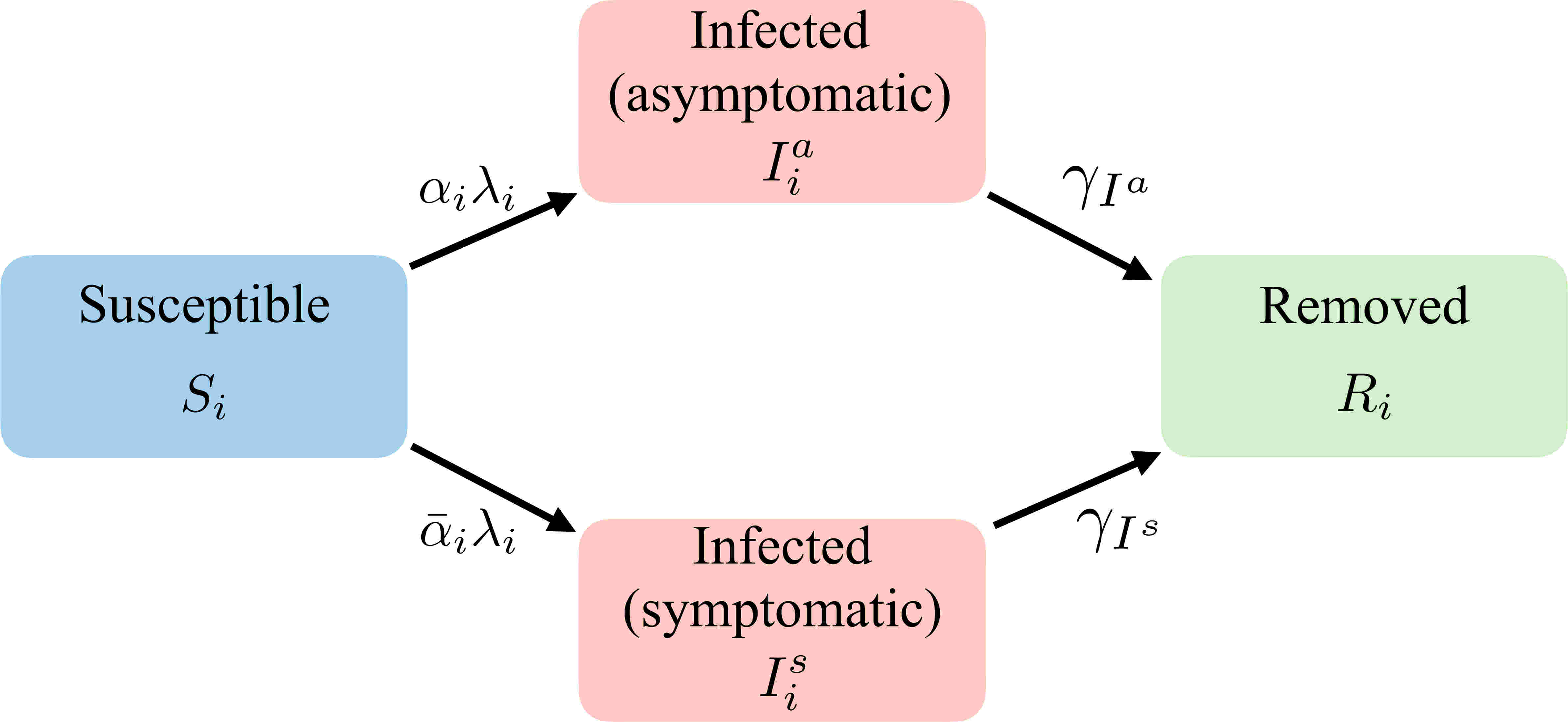
We now extend the classic SIR model to an SIIR model, where the infective class has been divided in asymptomatic $I_{i}^{a}$ and symptomatic $I_{i}^{s}$. We assume that the rate of infection of a susceptible individual in age group $i$ is

$$\lambda_{i}(t)=\beta\sum_{j=1}^{M}\left(C_{ij}^{a}(t)\frac{I_{j}^{a}}{N_{j}}+C_{ij}^{s}(t)\frac{I_{j}^{s}}{N_{j}}\right),\quad i,j=1,\ldots M$$ (1)

where $\beta$ is the probability of infection on contact (assumed intrinsic to the pathogen) and $C_{ij}^{a}$ and $C_{ij}^{s}$ are, respectively, the number of contacts between asymptomatic and symptomatic infectives in age-group $j$ with susceptibles in age-group $i$ (reflecting the structure of social contacts). We assume that symptomatic infectives reduce their contacts compared to asymptomatic infectives and set $C_{ij}^{s}=f^{s}C_{ij}^{a}\equiv f^{s}C_{ij}$, where $0\leq f^{s}\leq 1$ is the proportion of contacts that are now avoided by these self-isolating individuals (allowing also for compliance rates)

With these assumptions the progress of the epidemic is governed by the age-structured SIIR model. Figure 1 shows the schematic. The deterministic limit is given as,

$$\dot{S_{i}} =-\lambda_{i}(t)S_{i},$$

$$\dot{I}_{i}^{a} =\alpha_{i}\lambda_{i}(t)S_{i}-\gamma_{I^{a}}I_{i}^{a},$$ (2)

$$\dot{I}_{i}^{s} =\bar{\alpha_{i}}\lambda_{i}(t)S_{i}-\gamma_{I^{s}}I_{i}^{s},$$

$$\dot{R}_{i} =\gamma_{I^{a}}I_{i}^{a}+\gamma_{I^{s}}I_{i}^{s}.$$

Here $\gamma_{I^{a}}$ is the removal rate for asymptomatic infectives, $\gamma_{I^{s}}$ is the removal rate for symptomatic infectives, $\alpha_{i}$ is the fraction of asymptomatic infectives.

4 SEIR

Figure 1: Schematic of the SEIR model. The parameters for this model are: $\boldsymbol{\theta}=(\beta,\gamma_{I},\gamma_{E})$. The class SEIR can be instantiated in PyRoss using pyross.deterministic.SEIR.

The SIR model does not model the incubation period of a virus. This can be included by adding to the SIR model an exposed E compartment (to give an age-structured SEIR model) [45, 3, 46, 47]. Figure 1 shows the schematic of the SEIR model. The deterministic ODE giving its time-evolution is

$$\dot{S_{i}} =-\lambda_{i}(t)S_{i},$$

$$\dot{E}_{i} =\lambda_{i}(t)S_{i}-\gamma_{E}E_{i}$$

$$\dot{I}_{i} =\gamma_{E}E_{i}-\gamma_{I}I_{i},$$ (1)

$$\dot{R}_{i} =\gamma_{I}I_{i}.$$

The rate of infection of a susceptible individual in age group $i$ is

$$\lambda_{i}(t)=\beta\sum_{j=1}^{M}\left(C_{ij}(t)\frac{I_{j}}{N_{j}}\right),\quad i,j=1,\ldots M$$ (2)

5 SEIR with stages (SEkIkR)

Figure 1: Schematic of the SEIR with stages (SEkIkR) model. The parameters for this model are: $\boldsymbol{\theta}=(k_{I},k_{E},\beta,\gamma_{I},\gamma_{E})$. The class SEkIkR can be instantiated in PyRoss using pyross.deterministic.SEkIkR.

The SEIR model considers only four mutually exclusive epidemiological states: $S,E,I,R$. This leads to an exponentially distributed residence time in the incubating and infectious state. We use the same resolution as in SIkR model, see 2, to obtain a more realistic distribution of incubation and infectious times. The SEIR model can be extended to an age-structured $k-$staged SEkIkR model. Figure 1 shows the schematic. The ODE describing SEIR is:

$$\dot{S_{i}} =-\lambda_{i}(t)S_{i},$$

$$\dot{E}_{i}^{1} =\lambda_{i}(t)S_{i}-k_{E}\gamma_{E}E_{i}^{1}$$

$$\vdots$$

$$\dot{E}_{i}^{k} =k_{E}\gamma_{E}E_{i}^{k-1}-k_{E}\gamma_{E}E_{i}^{k}$$ (1)

$$\dot{I}_{i}^{1} =k_{E}\gamma_{E}E_{i}^{k}-k_{I}\gamma_{I}I_{i}^{1},$$

$$\vdots$$

$$\dot{I}_{i}^{k} =k_{I}\gamma_{I}I_{i}^{(k-1)}-k_{I}\gamma_{I}I_{i}^{k},$$

$$\dot{R}_{i} =k_{I}\gamma_{I}I_{i}^{k}.$$

The rate of infection of a susceptible individual in age group $i$ is

$$\lambda_{i}(t)=\beta\sum_{j=1}^{M}\sum_{n=1}^{k}C_{ij}(t)\frac{I_{j}^{n}}{N_{j}},$$ (2)

6 SEIIR

Figure 1: Schematic of the SEIIR model. The parameters for this model are: $\boldsymbol{\theta}=(\alpha_{i},\beta,\gamma_{E},\gamma_{I^{a}},\gamma_{I^{s}})$. The class SEIIR can be instantiated in PyRoss using pyross.deterministic.SEIR. Please note that both SEIIR and SEIR have been implemented as pyross.deterministic.SEIR in PyRoss as it possible to go from one to another by correct choice of parameters.

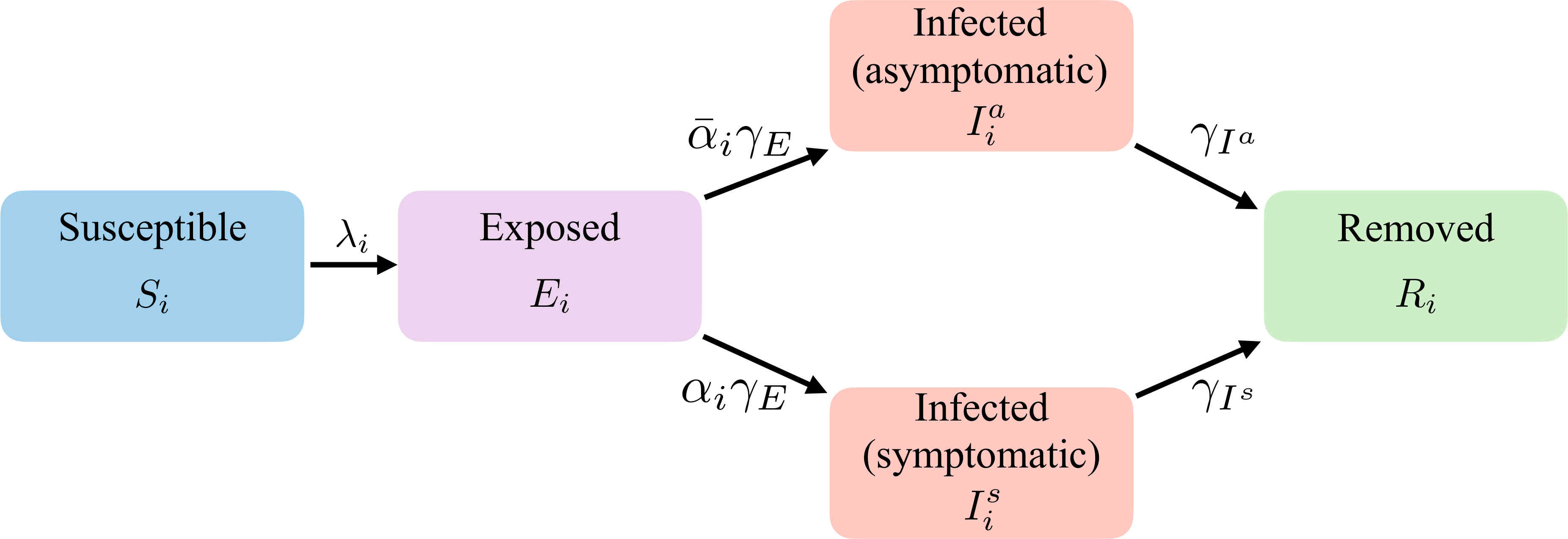
We now extend the classic SIR model to an SIIR model, where the infective class has been divided in asymptomatic $I_{i}^{a}$ and symptomatic $I_{i}^{s}$. We assume that the rate of infection of a susceptible individual in age group $i$ is

$$\lambda_{i}(t)=\beta\sum_{j=1}^{M}\left(C_{ij}^{a}\frac{I_{j}^{a}}{N_{j}}+C_{ij}^{s}\frac{I_{j}^{s}}{N_{j}}\right),$$ (1)

The deterministic dynamics is given by the following ODE:

$$\dot{S_{i}} =-\lambda_{i}(t)S_{i},$$

$$\dot{E}_{i} =\lambda_{i}(t)S_{i}-\gamma_{E}E_{i}$$

$$\dot{I}_{i}^{a} =\alpha_{i}\gamma_{E}E_{i}-\gamma_{I^{a}}I_{i}^{a},$$ (2)

$$\dot{I}_{i}^{s} =\bar{\alpha_{i}}\gamma_{E}E_{i}-\gamma_{I^{a}}I_{i}^{s},$$

$$\dot{R}_{i} =\gamma_{I^{a}}I_{i}^{a}+\gamma_{I^{s}}I_{i}^{s}.$$

7 SEIIR with stages (SEkIkIkR)

Figure 1: Schematic of the SEIIR with stages (SEkIkIkR) model. The parameters for this model are: $\boldsymbol{\theta}=(k_{I},k_{E},\alpha_{i},\beta,\gamma_{I^{a}},\gamma_{I^{s}},\gamma_{E})$. The class SEkIkIkR can be instantiated in PyRoss using pyross.deterministic.SEkIkIkR.

We now extend the SEIIR model to have stages in exposed, asymptomatic infectives, and symptomatic infectives classes. This is the the same resolution as in SIkR model, see 2, to obtain a more realistic distribution of incubation and infectious times. Figure 1 shows the schematic. The deterministic dynamics is given as

$$\dot{S_{i}} =-\lambda_{i}(t)S_{i},$$

$$\dot{E}_{i}^{1} =\lambda_{i}(t)S_{i}-k_{E}\gamma_{E}E_{i}^{1}$$

$$\vdots$$

$$\dot{E}_{i}^{k_{E}} =k_{E}\gamma_{E}E_{i}^{k_{E}-1}-k_{E}\gamma_{E}E_{i}^{k_{E}}$$ (1)

$$\dot{I}_{i}^{a1} =\alpha_{i}k_{E}\gamma_{E}E_{i}^{k}-k_{I}\gamma_{I^{a}}I_{i}^{a1},$$

$$\vdots$$

$$\dot{I}_{i}^{ak_{I}} =k_{I^{a}}\gamma_{I^{a}}I_{i}^{a(k_{I}-1)}-k_{I}\gamma_{I^{a}}I_{i}^{ak_{I}},$$

$$\dot{I}_{i}^{s1} =\bar{\alpha_{i}}k_{E}\gamma_{E}E_{i}^{k_{E}}-k_{I}\gamma_{I^{s}}I_{i}^{a1},$$ (2)

$$\vdots$$ (3)

$$\dot{I}_{i}^{sk_{I}} =k_{I}\gamma_{I^{s}}I_{i}^{s(k_{I}-1)}-k_{I}\gamma_{I^{s}}I_{i}^{sk_{I}},$$ (4)

$$\dot{R}_{i} =k_{I}\gamma_{I^{a}}I_{i}^{ak_{I}}+k_{I}\gamma_{I^{s}}I_{i}^{sk_{I}}.$$

We assume that the rate of infection of a susceptible individual in age group $i$ is

$$\lambda_{i}(t)=\beta\sum_{j=1}^{M}\sum_{n=1}^{k_{I}}\left(C_{ij}^{a}\frac{I_{j}^{an}}{N_{j}}+C_{ij}^{s}\frac{I_{j}^{sn}}{N_{j}}\right),$$ (5)

8 SEAIIR

Figure 1: Schematic of the SEAIIR model. The parameters for this model are: $\boldsymbol{\theta}=(\alpha_{i},\beta,\gamma_{E},\gamma_{A},\gamma_{I^{a}},\gamma_{I^{s}})$. The class SEAIIR can be instantiated in PyRoss using pyross.deterministic.SEAIR.

This model is an extension of the SEIR model, introducing the additional class $A$, which is both asymptomatic and infectious. In other words, this models shows what ensues if everyone who gets infected, undergoes a latency period where they are both asymptomatic and infectious. This class is potentially quite important, as there is some evidence that people are infectious before they start showing symptoms. The deterministic limit of this case

$$\dot{S}_{i} =-\lambda_{i}(t)S_{i}$$ (1)

$$\dot{E}_{i} =\lambda_{i}(t)S_{i}-\gamma_{E}E_{i}$$

$$\dot{A}_{i} =\gamma_{E}E_{i}-\gamma_{A}A_{i}$$

$$\dot{I}_{i}^{a} =\alpha_{i}\gamma_{A}A_{i}-\gamma_{I^{a}}I_{i}^{a}$$

$$\dot{I}_{i}^{s} =\bar{\alpha_{i}}\gamma_{A}A_{i}-\gamma_{I^{s}}I_{i}^{s}$$

$$\dot{R}_{i} =\gamma_{I^{a}}I_{i}^{a}+\gamma_{I^{s}}I_{i}^{s}$$

The rate of infection of a susceptible individual in age group $i$ is

$$\lambda_{i}(t)=\beta\sum_{j=1}^{M}\left(C_{ij}^{a}\frac{I_{j}^{a}}{N_{j}}+C_{ij}^{a}\frac{A_{j}}{N_{j}}+C_{ij}^{s}\frac{I_{j}^{s}}{N_{j}}\right),$$ (2)

The $A$ and $I^{a}$ classes should behave virtually the same (so their contact matrices should be equal). The two are kept distinct to keep track of the fact that some people remain asymptomatic even in the $I$ stage. Since it’s difficult to find data on the ratio of $I^{s}$ to $I^{a}$, it is possible to disregard the distinction and simply use $I$ instead.

9 SEAI8R

Figure 1: Schematic of the SEAI8R model. The class SEAI8R can be instantiated in PyRoss using pyross.deterministic.SEAI8R.

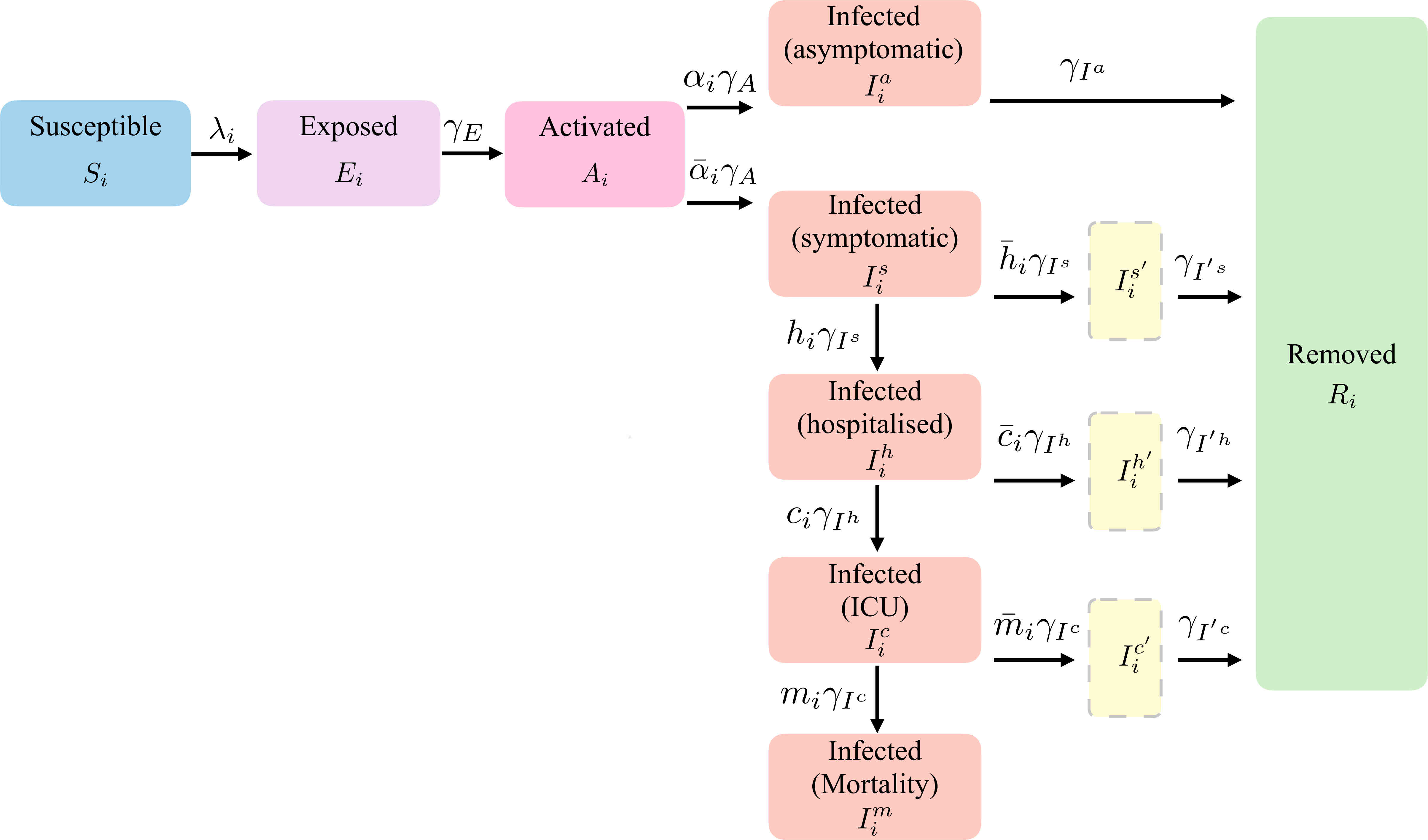
This model is an extension of the SEAIIR model. There are now six more types of infectives ($I_{i}^{h}$: infectives who are hospitalized, $I_{i}^{c}$: infectives who are in ICU, $I_{i}^{m}$: mortality due to the infection from ICU, $I_{i}^{s^{\prime}}:$ intermediate stage between symptomatic and removed, $I_{i}^{c^{\prime}}:$ intermediate stage between hospitalized and removed, and $I_{i}^{c^{\prime}}:$ intermediate stage between ICU and removed). The intermediate stages are needed to allow for a fast progression of the disease while retaining the longer recovery time and the ratios of people experiencing different levels of severity of the disease. Figure 1 shows the schematic. The deterministic dynamics if given by the following ODE:

$$\dot{S_{i}}=-\lambda_{i}(t)S_{i}+\sigma_{i},\qquad\dot{E}_{i}=\lambda_{i}(t)S_{i}-\gamma_{E}E_{i},\qquad\dot{A}_{i}=\gamma_{E}E_{i}-\gamma_{A}A_{i}$$

$$\dot{I}_{i}^{a}=\alpha_{i}\gamma_{A}A_{i}-\gamma_{I^{a}}I_{i}^{a},\qquad\dot{I}_{i}^{s}=\bar{\alpha_{i}}\gamma_{A}A_{i}-\gamma_{I^{s}}I_{i}^{s},\qquad\dot{I}_{i}^{s^{\prime}}=\bar{h}_{i}\gamma_{I^{s}}I_{i}^{s}-\gamma_{I^{s^{\prime}}}I_{i}^{s^{\prime}}$$

$$\dot{I}_{i}^{h}=h_{i}\gamma_{I^{s}}I_{i}^{s}-\gamma_{I^{h}}I_{i}^{h},\qquad\dot{I}_{i}^{h^{\prime}}=\bar{c}_{i}\gamma_{I^{h}}I_{i}^{h}-\gamma_{I^{h^{\prime}}}I_{i}^{h^{\prime}},\qquad\dot{I}_{i}^{c}=c_{i}\gamma_{I^{h}}I_{i}^{h}-\gamma_{I^{c}}I_{i}^{c},$$

$$\dot{I}_{i}^{c^{\prime}}=\bar{m}_{i}\gamma_{I^{c}}I_{i}^{c}-\gamma_{I^{c^{\prime}}}I_{i}^{c^{\prime}},\qquad\dot{I}_{i}^{m}=m_{i}\gamma_{I^{c}}I_{i}^{c},\qquad\dot{N}_{i}=\sigma_{i}-m_{i}\gamma_{I^{c}}I_{i}^{c}$$ (1)

$$\dot{R}_{i}=\gamma_{I^{a}}I_{i}^{a}+\gamma_{I^{s^{\prime}}}I_{i}^{s^{\prime}}+\gamma_{I^{h^{\prime}}}I_{i}^{h^{\prime}}+\gamma_{I^{c^{\prime}}}I_{i}^{c^{\prime}}.$$

The rate of infection of a susceptible individual in age group $i$ is

$$\lambda_{i}(t)=\beta\sum_{j=1}^{M}\left(C_{ij}^{a}\frac{I_{j}^{a}}{N_{j}}+C_{ij}^{a}\frac{A_{j}}{N_{j}}+C_{ij}^{s}\frac{I_{j}^{s}}{N_{j}}+C_{ij}^{h}\frac{I_{j}^{h}}{N_{j}}\right),$$ (2)

Here $\bar{h}_{i}=1-h_{i}$, $\bar{m}_{i}=1-m_{i}$, $C_{ij}^{s}=f^{s}C_{ij}^{a}\equiv f^{s}C_{ij}$ and $C_{ij}^{s}=f^{h}C_{ij}^{a}\equiv f^{h}C_{ij}$. We note the individuals can be removed at any stage from either of the eight infection classes.

10 SEAIIRQ

Figure 1: Schematic of the SEAIIRQ model. The parameters for this model are: $\boldsymbol{\theta}=(\alpha_{i},\beta,\gamma_{E},\gamma_{A},\gamma_{I^{a}},\gamma_{I^{s}},\tau_{E},\tau_{A},\tau_{I^{a}},\tau_{I^{s}})$. The class SEAIIRQ can be instantiated in PyRoss using pyross.deterministic.SEAIRQ.

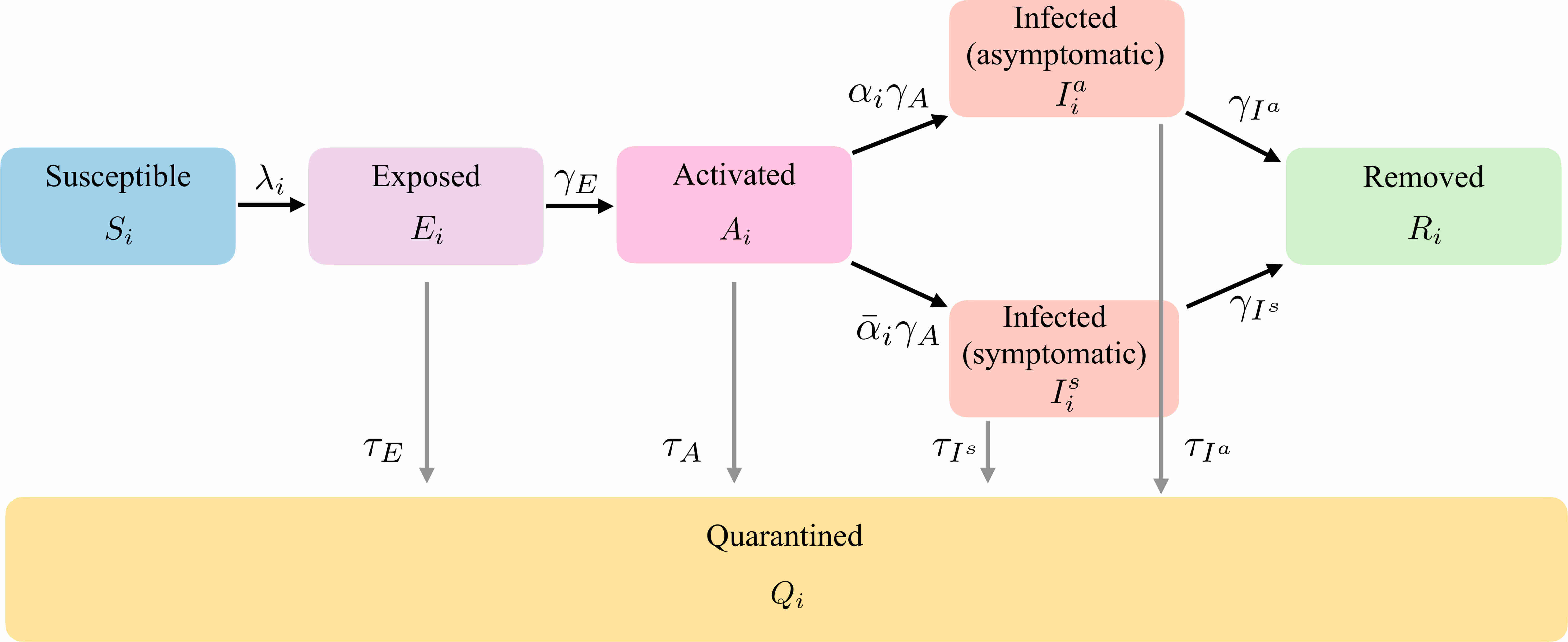
This model is an extension of the SEAIIR model. We introduce the $Q_{i}$ class, which may model individuals who have been tested and put into quarantine (and can therefore not infect anyone else). This point of $Q_{i}$ class is to model a possible an implementation of contact tracing in PyRoss. Figure 1 shows the schematic. The deterministic dynamics of the SEAIRQ model is given as:

$$\dot{S}_{i} =-\lambda_{i}(t)S_{i}$$ (1)

$$\dot{E}_{i} =\lambda_{i}(t)S_{i}-(\gamma_{E}+\tau_{E})E_{i}$$

$$\dot{A}_{i} =\gamma_{E}E_{i}-(\gamma_{A}+\tau_{A})A_{i}$$

$$\dot{I}_{i}^{a} =\alpha_{i}\gamma_{A}A_{i}-(\gamma_{I^{a}}+\tau_{I^{a}})I_{i}^{a}$$

$$\dot{I}_{i}^{s} =\bar{\alpha_{i}}\gamma_{A}A_{i}-(\gamma_{I^{s}}+\tau_{I^{s}})I_{i}^{s}$$

$$\dot{R}_{i} =\gamma_{I^{a}}I_{i}^{a}+\gamma_{I^{s}}I_{i}^{s}$$

$$\dot{Q}_{i} =\tau_{S}S_{i}+\tau_{E}E_{i}+\tau_{A}A_{i}+\tau_{I^{s}}I_{i}^{s}+\tau_{I^{a}}I_{i}^{a}$$

The rate of infection of a susceptible individual in age group $i$ is

$$\lambda_{i}(t)=\beta\sum_{j=1}^{M}\left(C_{ij}^{a}\frac{I_{j}^{a}}{N_{j}}+C_{ij}^{a}\frac{A_{j}}{N_{j}}+C_{ij}^{s}\frac{I_{j}^{s}}{N_{j}}\right),$$ (2)

Here $\tau_{E,A,I^{s},I^{a}}$ is the testing rate in the population, these are in general different for different classes. We have presumed that people in the incubation stage $E$ can also be tested.

11 SIIRS

Figure 1: Schematic of the SIIRS model. The parameters for this model are: $\boldsymbol{\theta}=(\alpha_{i},\beta,\gamma_{I^{a}},\gamma_{I^{s}},\epsilon)$. The class SIIRS can be instantiated in PyRoss using pyross.deterministic.SIRS.

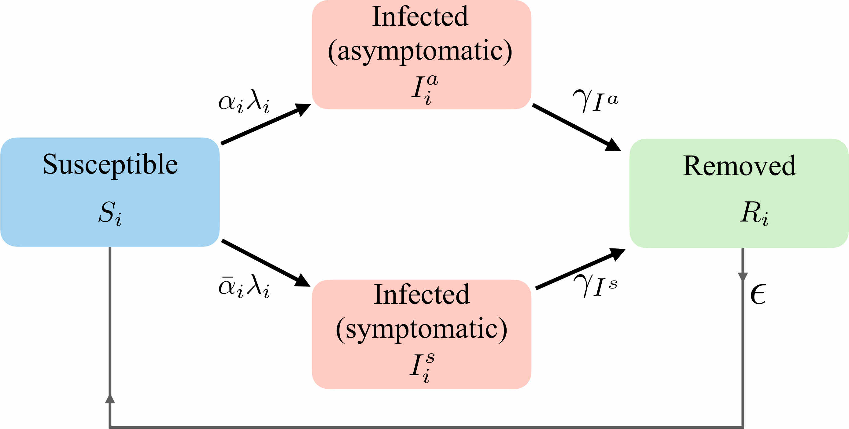
We now extend the age-structured SIR model to allow for removed persons to be susceptible and for change in the population of each age group. Figure 1 shows the schematic. The deterministic dynamics of the resulting SIRS model is:

$$\begin{aligned} \dot{S}_{i}&=-\lambda_{i}(t)S_{i}+\sigma_{i}+\epsilon(\gamma_{I^{a}}I_{i}^{a}+\gamma_{I^{s}}I_{i}^{s})\\ \dot{I}_{i}^{a}&=\alpha_{i}\lambda_{i}(t)S_{i}-\gamma_{I^{a}}I_{i}^{a}+l_{i}\\ \dot{I}_{i}^{s}&=\bar{\alpha_{i}}\lambda_{i}(t)S_{i}-\gamma_{I^{a}}I_{i}^{s}\\ \dot{R}_{i}&=\gamma_{I^{a}}I_{i}^{a}+\gamma_{I^{s}}I_{i}^{s}.\\ \dot{N}_{i}&=\sigma_{i}+l_{i}\end{aligned}$$ (1)

Here $\epsilon$ is fraction of removed who is susceptible. $\sigma_{i}$ denotes of the arrival of new susceptibles, while $l_{i}$ are new asymptomatic infectives. This means that $N_{i}$ is now dynamical. The rate of infection of a susceptible individual in age group $i$ is same as in the SIIR model.

12 Generic user-defined model

If the plethora of models described in the preceding sections are not enough, then PyRoss provides the additional class pyross.deterministic.Spp (pronounced “S plus plus”), which has the ability to simulate any generic compartmental model. The model is specified by providing a Python dictionary, and supports age-differentiated parameters. As an example, the SIR model, defined in the Spp class, is given in Fig.1.

⬇

model_spec = {

"classes" : ["S", "I", "R"],

"S" : {

"linear" : [],

"infection" : [ ["I", "-beta"] ]

},

"I" : {

"linear" : [ ["I", "-gamma"] ],

"infection" : [ ["I", "beta"] ]

},

"R" : {

"linear" : [ ["I", "gamma"] ],

"infection" : []

}

}

Figure 1: Definition of the Spp class. The Spp class can be instantiated in PyRoss using pyross.deterministic.Spp.

Currently, the Spp class supports the two types of terms which all the compartmental models above share: linear terms and infection terms. The class could be used to simulate any generic age-structured epidemiological compartment model, where the rates could be both time and state dependent.

Note that pyross.deterministic.Spp is designed with generality rather than optimality in mind. A model implemented using pyross.deterministic.Spp will in general perform worse than any of the corresponding hard-coded classes above.

Chapter 4 Applications

In this chapter, we provide illustrative examples of usage of the PyRoss library.

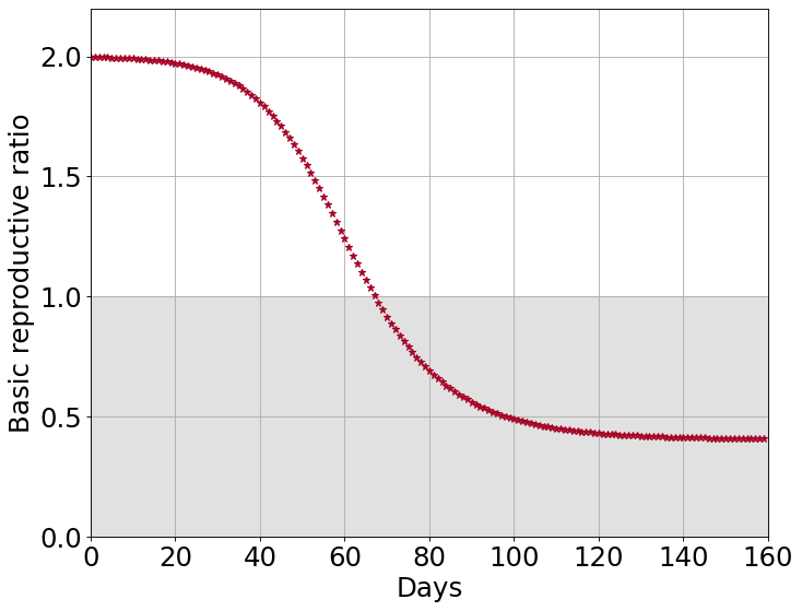
1 Basic reproductive ratio $\mathcal{R}_{0}$ from local rate of growth

Our first example is on computing the basic reproductive ratio $\mathcal{R}_{0}$ as a function of intervention measures. In a population of susceptibles $S_{i}$, the expected number of secondary infections arising from a single individual during the entire infectious period is defined as $\mathcal{R}_{0}$ [14, 48]. We obtain the basic reproductive ratio of the SIR model, defined in section 1, by linearising the dynamics about the disease-free fixed point, where $S_{i}=N_{i}$. The time evolution of infectives is governed by

$$\boldsymbol{J}=\gamma(\boldsymbol{L}-\boldsymbol{1}).$$ (1)

Here $\boldsymbol{1}$ is the identity matrix and

$$\boldsymbol{L}=\frac{\alpha\beta}{\gamma}C_{ij}\frac{N_{i}}{N_{j}}.$$

It is sufficient for the spectral radius of $\boldsymbol{L}$ to be greater than unity for the epidemic to grow. The $\mathcal{R}_{0}$ is then obtained as the spectral radius of $\boldsymbol{L}$ [14, 48]:

$$\mathcal{R}_{0}\equiv\rho(\boldsymbol{L})=\text{max}\{|\Lambda_{1}|,\ldots,|\Lambda_{M}|\}.$$ (2)

We can now extend the linearisation at any point in time $t$ by making the replacements $N_{i}$ $\longrightarrow$ $S_{i}(t)$ and $C_{ij}\longrightarrow C_{ij}(t)$ in the expression for $\boldsymbol{L}$, giving the time-dependent stability matrix $\boldsymbol{L}^{(t)}$ [16], and thus, define effective time-dependent basic reproductive ratio

$$\mathcal{R}_{\text{0}}^{\text{eff}}(t)\equiv\rho(\boldsymbol{L}^{(t)})=\text{max}\{|\Lambda_{1}^{(t)}|,\ldots,|\Lambda_{M}^{(t)}|\}$$ (3)

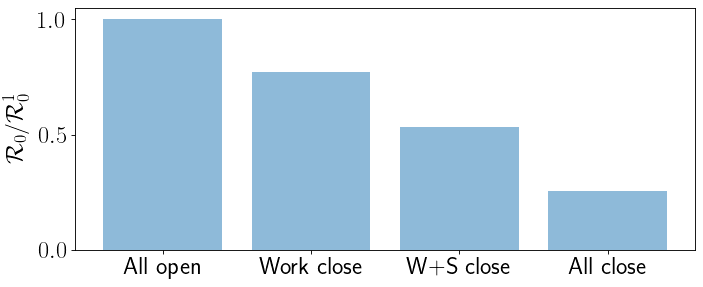
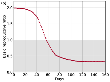
We now provide illustrative examples of measuring $\mathcal{R}_{0}$ and $\mathcal{R^{\text{eff}}}_{0}(t)$. In Fig.(1), we obtain the basic reproductive ration as intervention measures are changed.

⬇

import pyross

import matplotlib.pyplot as plt, numpy as np

M=16 ## number of age classes

my_data = np.genfromtxt(’UK.csv’, delimiter=’,’, skip_header=1)

Ni = (my_data[:,1]+my_data[:,2])[0:M]

# contact structure of the UK

ukCH, ukCW, ukCS, ukCO = pyross.contactMatrix.UK()

aH, aW, aS, aO = 1, 1, 1, 1

CH, CW, CS, CO = aH*ukCH, aW*ukCW, aS*ukCS, aO*ukCO

beta = 1 # the probability of infection on contact

gIa = 1./7 # removal rate of asymptomatic infectives

gIs = 1./7 # removal rate of symptomatic infectives

alpha = 0. # asymptomatic fraction

fsa = 1 # suppresion of contact by symptomatics

parameters = {’alpha’:alpha,’beta’:beta, ’gIa’:gIa,’gIs’:gIs,’fsa’:fsa, ’M’:M, ’Ni’:Ni}

contactMatrix = pyross.contactMatrix.SIR(CH, CW, CS, CO)

r0UK1 = contactMatrix.basicReproductiveRatio(parameters)

#switch off contacts at work

aH, aW, aS, aO = 1, 0, 1, 1

CH, CW, CS, CO = aH*ukCH, aW*ukCW, aS*ukCS, aO*ukCO

contactMatrix = pyross.contactMatrix.SIR(CH, CW, CS, CO)

r0UK2 = contactMatrix.basicReproductiveRatio(parameters)

#switch off contacts at work and school

aH, aW, aS, aO = 1, 0, 0, 1

CH, CW, CS, CO = aH*ukCH, aW*ukCW, aS*ukCS, aO*ukCO

contactMatrix = pyross.contactMatrix.SIR(CH, CW, CS, CO)

r0UK3 = contactMatrix.basicReproductiveRatio(parameters)

#switch off all contacts but at home

aH, aW, aS, aO = 1, 0, 0, 0

CH, CW, CS, CO = aH*ukCH, aW*ukCW, aS*ukCS, aO*ukCO

contactMatrix = pyross.contactMatrix.SIR(CH, CW, CS, CO)

r0UK4 = contactMatrix.basicReproductiveRatio(parameters)

r0 = np.array([r0UK1, r0UK2, r0UK3, r0UK4])/r0UK1

plt.bar(range(r0.size), r0, align=’center’, alpha=0.5);

plt.ylabel(r’$\mathcal R_0/\mathcal R^{{1}}_0$’)

labelY= (’All open’, ’Work close’, ’School close’, ’All close’ );

plt.xticks(range(r0.size),labelY);

Figure 1: The basic reproductive ratio as a function of intervention measures. The y-axis is normalized by the case without no intervention measures. Here ‘W+S close’ means both work and school are closed and $\mathcal{R}_{0}^{1}$ is the basic reproductive ration without any intervention measure.

2 Beyond $\mathcal{R}_{0}$: Kreiss constant $\mathcal{K}(\boldsymbol{J})$

In the previous section, we used linearisation to study growth of epidemic. The prediction made by linearised theory is based on the fact that the growth rate of a linear system is exponential in the largest eigenvalue. This is well known in the epidemiology community, where the value of $\mathcal{R}_{0}$ is used as a measure of how dangerous an epidemic will become and on what timescale. On the other hand, far less well known is the transient effect due to non-normality of $\boldsymbol{J}$ on the initial dynamics. There have been some papers [49, 50] in the ecology community on this effect in the context of population dynamics. The best way to understand why non-normality can be important is through an instructive example. Let $\boldsymbol{x}=\bar{\boldsymbol{x}}+\boldsymbol{u}$,

$$\frac{d\boldsymbol{u}}{dt}=\boldsymbol{J}(t,\boldsymbol{\theta},\bar{\boldsymbol{x}})\cdot\boldsymbol{u}$$

Consider,

$$\boldsymbol{J}=\begin{pmatrix}-1&500\\ 0&-2\end{pmatrix}$$

⬇

import pyross

import numpy as np, matplotlib.pyplot as plt

import scipy.linalg as spl

from scipy.integrate import solve_ivp

from pyross.contactMatrix import characterise_transient

M = 2 # the SIR model has no age structure

N = 100000 # the total population

Ni = np.zeros((M)) # population in each group

fi = np.zeros((M)) # fraction of population in age age group

fi = np.array((0.25, 0.75))

for i in range(M):

Ni[i] = fi[i]*N

beta = 0.02 # infection rate

gamma = 0.007

gIa = gamma # removal rate of asymptomatic infectives

gIs = gamma # removal rate of symptomatic infectives

alpha = 0 # fraction of asymptomatic infectives

fsa = 1 # the self-isolation parameter

Ia0 = np.array([0,0]) # the SIR model has only one kind of infective

Is0 = np.array([1,.1]) # we take these to be symptomatic

R0 = np.array([0,0]) # and assume there are no removed individuals initially

S0 = Ni-Ia0-Is0-R0

# set the contact structure

C11, C22, C12 = 1,1,4

C = np.array(([C11, C12], [C12*fi[1]/fi[0], C22]))

def contactMatrix(t):

return C

# duration of simulation and data file

Tf = 160; Nt=160;

# instantiate model

parameters = {’alpha’:alpha, ’beta’:beta, ’gIa’:gIa, ’gIs’:gIs,’fsa’:fsa}

model = pyross.deterministic.SIR(parameters, M, Ni)

# simulate model

data = model.simulate(S0, Ia0, Is0, contactMatrix, Tf, Nt)

# matrix for linearised dynamics

C=contactMatrix(0)

A=((beta*C-gamma*np.identity(len(C))).T*fi).T/fi

mcA=pyross.contactMatrix.characterise_transient(A, ord=1)

AP = A-np.max(np.linalg.eigvals(A))*np.identity(len(A))

mcAA = pyross.contactMatrix.characterise_transient(AP,ord=1)

# plot the data and obtain the epidemic curve

Sa =data[’X’][:,:1].flatten(); Sk=data[’X’][:,1:M].flatten()

Isa =data[’X’][:,2*M:2*M+1].flatten(); Isk=data[’X’][:,2*M+1:3*M].flatten()

St=Sa+Sk; It=Isa+Isk

# It = np.sqrt(Isa**2 + Isk**2)

t = data[’t’]

fig = plt.figure(num=None, figsize=(10, 8), dpi=80, facecolor=’w’, edgecolor=’k’)

plt.fill_between(t, 0, St/N, color="#348ABD", alpha=0.3)

plt.plot(t, St/N, ’-’, color="#348ABD", label=’$S$’, lw=4)

plt.fill_between(t, 0, It/N, color=’#A60628’, alpha=0.3)

plt.plot(t, It/N, ’-’, color=’#A60628’, label=’$I$’, lw=4)

Rt=N-St-It; plt.fill_between(t, 0, Rt/N, color="dimgrey", alpha=0.3)

plt.plot(t, Rt/N, ’-’, color="dimgrey", label=’$R$’, lw=4)

plt.autoscale(enable=True, axis=’x’, tight=True)

###Estimate from Kreiss constant

plt.plot(t,mcAA[2]*It[0]*np.exp(mcA[0]*t)/N,’-’, color="green",

label=’$Estimate$’, lw=4)

plt.yscale(’log’); plt.xlabel("time"); plt.ylabel("% of population");

plt.legend(fontsize=26); plt.grid(); plt.show()

def linear_system(t, x, A): return A@x

A2 = np.array([[3,2],[9,4]])

x0, tf = [1,1], 1

ivp_exp = solve_ivp(linear_system, (0,tf), x0, args=[A2], t_eval=np.arange(0,tf,.1))

t=ivp_exp.t

Gamma = A2 - np.max(spl.eigvals(A2))*np.identity(len(A2))

mcA2 = characterise_transient(Gamma)

ivp_exp2 = solve_ivp(linear_system, (0,tf), x0, args=[Gamma], t_eval=np.arange(0,tf,.01))

f, ax = plt.subplots()

plt.plot(ivp_exp2.t,spl.norm(ivp_exp2.y.T, axis=1)/spl.norm(x0))

ax.set_xlabel("time"); ax.set_ylabel(r’$|u|/|u_0|$’)

ax.plot(t, np.exp(mcA2[0]*t),"--",color="darkgreen")

ax.set_ylim((-.1,np.max(spl.norm(ivp_exp2.y.T, axis=1)/spl.norm(x0))*1.1))

t_trunc = t[np.where(t<mcA2[3])]

ax.plot(t_trunc,np.exp(mcA2[1]*t_trunc),"--",color="orange")

plt.axhline(y=mcA2[2],linestyle="dotted",color="black")

plt.ylim([.98,1.4]); plt.annotate(r’Long time behaviour $\alpha (\Gamma)$’, [.2,1.01])

plt.annotate(r’Initial growth rate $\omega (\Gamma)$’,[.0,1.05], rotation=68)

plt.annotate(r’Kreiss constant $\mathcal{K} (\Gamma)$’, [.4,1.3]); plt.show()

(a)	(b)

Figure 1: Effect of non-normality on the dynamics. (a) The evolution of the associated : (a) The evolution of the associated . The non-normality of $\boldsymbol{C}$ results in a greater total number of infected, plotted in green. . The system quickly saturates the Kreiss bound and asymptotically tends towards normal evolution along it. (b) the 2-age structured SIR model with contact matrix

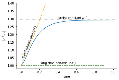
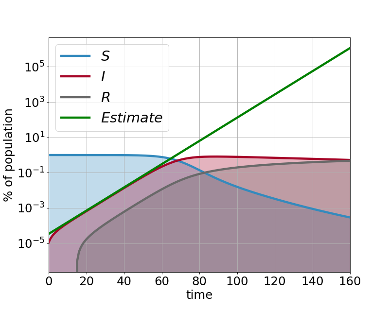
Obviously the eigenvalues are $-1,-2$ so a simple eigenvalue criterion would expect an exponential decay of any initial perturbations. However, let $\boldsymbol{u}_{0}=\left(0,1\right)$ and it is obvious that $|\boldsymbol{u}|$ is dramatically magnified in value. After a long enough time, the system will obviously decay to $0$ but in a non-linear system, transient amplification may have a dramatic effect on the long term dynamics if a system is only locally stable around some fixed point [51, 52]. The behaviour results from the non-normality of $\boldsymbol{J}$. Normal matrices are defined as $\boldsymbol{J}\boldsymbol{J}^{T}=\boldsymbol{J}^{T}\boldsymbol{J}$, which, by the spectral theorem, is the criterion for diagonalisability. Obviously eigenvalues alone cannot hope to encapsulate the full picture here. Here we show these effects can be encapsulated by the introduction of a single new multiplicative parameter and can be used to better understand the initial growth dynamics.

The transient is best characterized by the Kreiss constant $\mathcal{K}(\boldsymbol{J})$ which provides a lower bound to the maximum amplitude of a system evolving under $\boldsymbol{J}$ [53, 51, 49]. For a system that grows with time, the “extra increase” can be estimated by

$$\mathcal{K}(\boldsymbol{J}-\lambda_{\text{Max}}\left(\boldsymbol{J}\right)),$$

The associated system $\dot{\boldsymbol{u}}=\left(\boldsymbol{J}-\lambda_{Max}\boldsymbol{I}\right)\boldsymbol{u}=\boldsymbol{\Gamma}\boldsymbol{u}$ has the solution

$$u(t)=\frac{e^{\boldsymbol{J}t}}{e^{\lambda_{\text{Max}}t}}u(0)\underset{t\rightarrow\infty}{\rightarrow}\mathcal{K}(\boldsymbol{\Gamma})u(0).$$

In practice, the bound is well saturated over the time scale of the transient $\tau$ which is usually much faster than any other dynamics of the system (and can be estimated from pseudospectral methods [53] )

$$u(t)\underset{t\rightarrow\tau}{\rightarrow}\mathcal{K}(\boldsymbol{\Gamma})u(0)$$

Thus, the solution to our initial equation $\dot{u}=\boldsymbol{J}u$ can be estimated as

$$u(t)=e^{\lambda_{\text{Max}}t}\mathcal{K}(\boldsymbol{\Gamma})u(0).$$ (1)

In summary, the maximum eigenvalue and the Kreiss constant of the associated system together characterise the initial growth of non-normal evolution as seen in Eq.(1) and 1. This new parameter acts as an amplification of the initial conditions based on the degree of non-normality of our network and is general for any type of network, for example age structure or geographical information.

3 Stochastic sampling

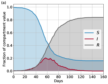
We now illustrate the usage of PyRoss for stochastic sampling of epidemics.

⬇

import numpy as np

import pyross

import matplotlib.pyplot as plt

M = 1 # the SIR model has no age structure

Ni = 1000*np.ones(M) # so there is only one age group

N = np.sum(Ni) # and the total population is the size of this age group

beta = 0.2 # infection rate

gIa = 0.1 # removal rate of asymptomatic infectives

gIs = 0.1 # removal rate of symptomatic infectives

alpha = 0 # fraction of asymptomatic infectives

fsa = 1 # self-isolation of symtomatic infectives

Ia0 = np.array([0]) # the SIR model has only one kind of infective

Is0 = np.array([5]) # we take these to be symptomatic

R0 = np.array([0]) # and assume there are no removed individuals initially

S0 = N-(Ia0+Is0+R0) # so that the initial susceptibles are obtained from S + Ia + Is + R = N

# there is no contact structure

def contactMatrix(t):

return np.identity(M)

# duration of simulation and data file

Tf = 160; Nt=160;

# instantiate model

parameters = {’alpha’:alpha, ’beta’:beta, ’gIa’:gIa, ’gIs’:gIs,’fsa’:fsa}

model = pyross.stochastic.SIR(parameters, M, Ni)

# simulate model

data = model.simulate(S0, Ia0, Is0, contactMatrix, Tf, Nt)

# plot the compartments

pyross.utils.plotSIR(data)

# plot the basic reproductive ratio as a function of time

C=np.identity(M)

contactMatrix = pyross.contactMatrix.SIR(0.25*C, 0.25*C, 0.25*C, 0.25*C)

r0de = contactMatrix.basicReproductiveRatio(data, state=’dynamic’)

t = data[’t’]

plt.fill_between(t, 0, t*0+1, color="dimgrey", alpha=0.2)

plt.plot(r0de, ’*’, color=’#A60628’)

plt.xlabel(’Days’); plt.grid()

plt.ylabel(’Basic reproductive ratio’)

plt.autoscale(enable=True, axis=’x’, tight=True);

plt.yticks(np.arange(0, 3, step=0.5)); plt.ylim(0,2.2);

plt.show()

Figure 1: A stochastic realisation of the SIR model, c.f. example 3. Subplot (a) shows a resulting epidemic curve, i.e. a plot of the number of susceptibles, infectives and removed as a function of time. Subplot (b) depicts the corresponding basic reproductive ratio.

4 Deterministic integration

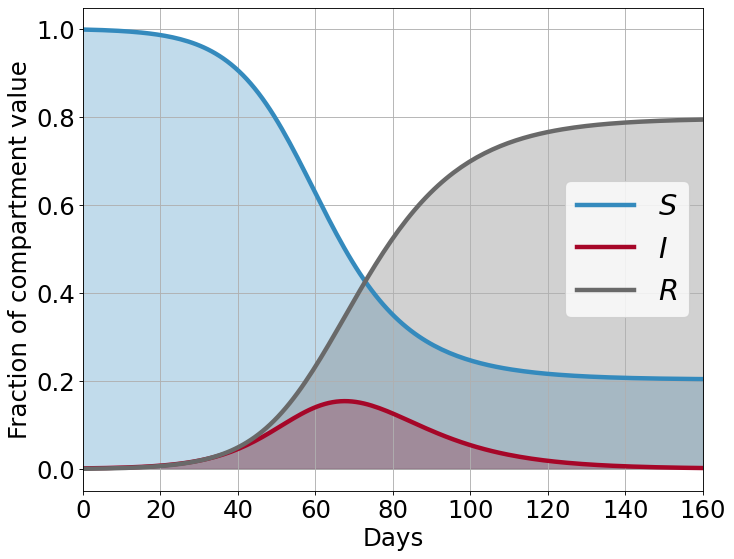
We now illustrate the usage of PyRoss for deterministic sampling of epidemics.

⬇

import numpy as np

import pyross

import matplotlib.pyplot as plt

M = 1 # the SIR model has no age structure

Ni = 1000*np.ones(M) # so there is only one age group

N = np.sum(Ni) # and the total population is the size of this age group

beta = 0.2 # infection rate

gIa = 0.1 # recovery rate of asymptomatic infectives

gIs = 0.1 # recovery rate of symptomatic infectives

alpha = 0 # fraction of asymptomatic infectives

fsa = 1 # self-isolation of symtomatic infectives

Ia0 = np.array([0]) # the SIR model has only one kind of infective

Is0 = np.array([1]) # we take these to be symptomatic

R0 = np.array([0]) # and assume there are no removed individuals initially

S0 = N-(Ia0+Is0+R0) # so that the initial susceptibles are obtained from S + Ia + Is + R = N

# there is no contact structure

def contactMatrix(t):

return np.identity(M)

# duration of simulation and data file

Tf = 160; Nt=160;

# instantiate model

parameters = {’alpha’:alpha, ’beta’:beta, ’gIa’:gIa, ’gIs’:gIs,’fsa’:fsa}

model = pyross.deterministic.SIR(parameters, M, Ni)

# simulate model

data = model.simulate(S0, Ia0, Is0, contactMatrix, Tf, Nt)

# plot the compartments

pyross.utils.plotSIR(data)

# plot the basic reproductive ratio as a function of time

C=np.identity(M); contactMatrix = pyross.contactMatrix.SIR(0.25*C, 0.25*C, 0.25*C, 0.25*C)

r0de = contactMatrix.basicReproductiveRatio(data, state=’dynamic’)

plt.plot(r0de, ’*’, color=’#A60628’)

Figure 1: A deterministic realisation of the SIR model, c.f. example 4. The left panel shows a resulting epidemic curve, i.e. a plot of the number of susceptibles, infectives and removed as a function of time. The right panel depicts the corresponding basic reproductive ratio.

5 Bayesian inference and forecasting

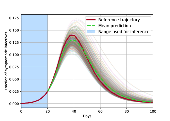
In this example, a trajectory of an SIIR model with two age groups is generated using pyross.stochastic. Based on the first 20 datapoints of the trajectory, pyross.inference is then used to infer the parameters of the time series. Finally, using pyross.forecast, predictions based the inferred parameters are made and compared to the original SIIR trajectory.

⬇

import numpy as np

import matplotlib.pyplot as plt

import pyross

# 1. Define model

# number of age groups and total population

M = 2 # the population has two age groups

N = 5e4 # and this is the total population

# exact parameters of reference trajectory

beta = 0.02 # infection rate

gIa = 1./7 # removal rate of asymptomatic infectives

gIs = 1./7 # removal rate of asymptomatic infectives

alpha = 0.2 # fraction of asymptomatic infectives

fsa = 0.8 # self-isolation of symtomatic infectives

# set the age structure

fi = np.array([0.25, 0.75]) # fraction of population in age age group

Ni = N*fi

# set up initial condition

Ia0 = np.array([10, 10]) # each age group has asymptomatic infectives

Is0 = np.array([10, 10]) # and also symptomatic infectives

R0 = np.array([0, 0]) # there are no removed individuals initially

S0 = Ni - (Ia0 + Is0 + R0) # initial number of susceptibles

# set the contact matrix

C = np.array([[18., 9.], [3., 12.]])

contactMatrix = lambda t: C

# 2. Use pyross stochastic to generate reference trajectory

Tf = 100; Nf = Tf+1 # reference trajectory is 100 days long

parameters = {’alpha’:alpha, ’beta’:beta, ’gIa’:gIa, ’gIs’:gIs,’fsa’:fsa}

sto_model = pyross.stochastic.SIR(parameters, M, Ni)

data = sto_model.simulate(S0, Ia0, Is0, contactMatrix, Tf, Nf)

data_array = data[’X’]

# 3. Run inference on the first 20 days

# create array with first 20 days of data

Tf_inf = 20; Nf_inf = Tf_inf + 1

data_inf = (data_array/N)[:Nf_inf]

# parameters for inference

ftol = 1e-6

steps = 101

estimator = pyross.inference.SIR(parameters, M, fi, int(N), steps)

# initial guesses, bounds, and initial standard deviation for solver

alpha_g = 0.15

alpha_std = 0.2

alpha_bounds = (1e-3, 0.5)

beta_g = 0.05

beta_std = 0.1

beta_bounds = (1e-3, 1)

gIa_g = 0.13

gIa_std = 0.1

gIa_bounds = (1e-3, 1)

gIs_g = 0.15

gIs_std = 0.1

gIs_bounds = (1e-3, 1)

guess = np.array([alpha_g, beta_g, gIa_g, gIs_g])

stds = np.array([alpha_std, beta_std, gIa_std, gIs_std])

bounds = np.array([alpha_bounds, beta_bounds, gIa_bounds, gIs_bounds])

keys = [’alpha’, ’beta’, ’gIa’, ’gIs’]

params = estimator.infer_parameters(keys, guess, stds, bounds, data_inf, Tf_inf, Nf_inf, contactMatrix,

global_max_iter=20, global_ftol_factor=10,

verbose=True)

print(params)

# for forecasting we also need the covariance matrix

hess = estimator.compute_hessian(keys, params, guess, stds,

data_inf, Tf_inf, Nf_inf, contactMatrix)

cov = np.linalg.inv(hess)

# 4. Run forecast using inferred parameters and their covariance

# instantiate model

parameters = {’alpha’: params[0], ’beta’: params[1],

’gIa’: params[2], ’gIs’: params[3],’fsa’:fsa,’cov’:cov}

model_forecast = pyross.forecast.SIR(parameters, M, Ni)

# initial condition for forecast is final state from inference

S0_fc = data_inf[-1,:M]*N

Ia0_fc = data_inf[-1,M:2*M]*N

Is0_fc = data_inf[-1,2*M:]*N

# run forecast

Tf_fc = Tf - Tf_inf; Nf_fc = Tf_fc+1 # simulation time for forecast

Ns = 500 # number of forecasting samples

result_fc = model_forecast.simulate(S0_fc, Ia0_fc, Is0_fc,

contactMatrix, Tf_fc, Nf_fc,Ns=Ns)

trajectories_fc = result_fc[’X’]

t_fc = result_fc[’t’] + Tf_inf

# 5. Visualise result: plot fraction of symptomatic infectives

traj_ref = np.sum(data_array[:,2*M:],axis=-1) # reference trajectory

trajs_fc = np.sum(trajectories_fc[:,2*M:],axis=1) # predictions

mean_fc = np.mean( trajs_fc, axis=0) # mean prediction

fig, ax = plt.subplots(1,1,figsize=(7,5))

ax.axvspan(0, Tf_inf,label=’Range used for inference’,

alpha=0.3,color=’dodgerblue’)

for i,e in enumerate(trajs_fc): # plot all forecasting trajectories

ax.plot(t_fc,e/N,alpha=0.1)

ax.plot(traj_ref/N,lw=3,color=’#A60628’,label=’Reference trajectory’)

ax.plot(t_fc,mean_fc/N,

ls=’--’,color=’limegreen’,label=’Mean prediction’,lw=3)

ax.set_xlim(0,np.max(t_fc))

ax.set_xlabel(r’Days’)

ax.set_ylabel(’Fraction of symptomatic infectives’)

ax.legend(loc=’upper right’,fontsize=12)

plt.grid(); plt.show()

plt.close(fig)

Figure 1: Bayesian inference and forecasting. Example 5 creates a trajectory (solid red line), estimates the model parameters based on the beginning of the trajectory (blue shaded region), and uses the estimated parameters to make predictions for the future time evolution (thin colored lines, with mean given by a thick dashed line).

6 Effect of event-driven NPI

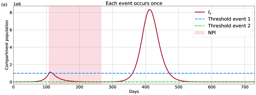
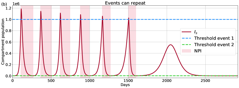
In this example, an event-driven protocol is defined: Once the number of symptomatic infectives exceeds a threshold, the contact matrix is reduced to the home contact; then, once the number of infectives falls below another threshold, the original contact matrix is restored. For an SEkIkIkR model with 16 age groups based on the UK age structure, and UK contact matrices, we run this protocol in two variations: First, we allow every event to happen at most one time; in the second run, we allow events to repeat. Note that while this example employs UK age groups and contact structure, the model parameters are not fitted to real epidemiological data.

⬇

import numpy as np

import matplotlib.pyplot as plt

import pyross

# 1. Load age structure and contact matrices of the UK

M=16 # number of age classes

# load age structure

my_data = np.genfromtxt(’../data/age_structures/UK.csv’,

delimiter=’,’, skip_header=1)

aM, aF = my_data[:, 1], my_data[:, 2]

Ni0=aM+aF

Ni = Ni0[:M] # consider first M age groups in data

N=np.sum(Ni) # total population is sum over all age groups

# get individual contact matrices

CH, CW, CS, CO = pyross.contactMatrix.UK()

# without interventions, the contact matrix is the sum of those

C = CH + CW + CS + CO

# 2. Define model

# parameters

alpha= 0.3 # fraction of symptomatics who self-isolate

beta = 0.0165 # probability of infection on contact

gE = 1/2.72 # recovery rate of exposeds

kI = 4; # # of stages of I class

kE = 4; # # of stages of E class

gIa = 1./7 # recovery rate of asymptomatic infectives

gIs = 1./17.76 # recovery rate of symptomatic infectives

fsa = 0.8 # the self-isolation parameter

# set up initial condition

S0 = np.zeros(M)

I0 = np.zeros((kI,M));

E0 = np.zeros((kE,M));

for i in range(kI):

I0[i, 6:13]=14; I0[i, 2:6]=13

for i in range(kE):

E0[i, 0:16]=14

for i in range(M) :

S0[i] = Ni[i] - np.sum(I0[:,i]) - np.sum(E0[:,i])

I0 = np.reshape(I0, kI*M)/kI;

E0 = np.reshape(E0, kE*M)/kE;

# 3. Define events and corresponding contact matrices

lockdown_threshold_1 = 1e6

lockdown_threshold_2 = 2000

#

events = []

contactMatrices = []

# Note that the event functions take a vector argument

# "xt" instead of a tuple (S, E0, Ia, Is).

# When defining the event functions for the SEkIkIkR

# model, the following correspondence has to be used:

# S == xt[ : M]

# E == xt[1*M :(1+kE)*M]

# Ia == xt[(1+kE)*M :(1+kE+kI)*M]

# Is == xt[(1+kE+kI)*M:(1+kE+kI+kI)*M]

# (For any model, the order for the event functions is

# exactly the same as in the arguments of model.simulation)

# This is a dummy event which will never occur;

# it is used to set the initial contact matrix

def event0(t,xt):

return t + 1

event0.direction = +1

events.append(event0)

contactMatrices.append( C )

# Lockdown on

def event1(t,xt):

return np.sum(xt[(1+kE+kI)*M:(1+kE+2*kI)*M]) - lockdown_threshold_1

event1.direction = +1 # need to pass threshold from below for event

events.append(event1)

contactMatrices.append( CH ) # only home contact matrix

# Lockdown off

def event2(t,xt):

return np.sum(xt[(1+kE+kI)*M:(1+kE+2*kI)*M]) - lockdown_threshold_2

event2.direction = -1 # need to pass threshold from above for event

events.append(event2)

contactMatrices.append( C )

# 4. Run pyross.control simulation twice: Once with events only

# occuring once, and once with events possibly several times

# instantiate model

parameters = {’beta’:beta, ’gE’:gE, ’gIa’:gIa, ’gIs’:gIs,

’kI’:kI, ’kE’ : kE, ’fsa’:fsa, ’alpha’:alpha}

model = pyross.control.SEkIkIkR(parameters, M, Ni)

# Run 1: each event only occurs once

Tf = 2*365 # 2 years

Nt = (Tf +1)*10 # return 10 datapoints per day

result_1 = model.simulate(S0, E0, 0*I0, I0,

events=events,contactMatrices=contactMatrices,

Tf=Tf, Nf=Nt,events_repeat=False)

# Run 2: events can repeat

Tf = 8*365 # 8 years

Nt = (Tf +1)*10 # return 10 datapoints per day

result_2 = model.simulate(S0, E0, 0*I0, I0,

events=events,contactMatrices=contactMatrices,

Tf=Tf, Nf=Nt,events_repeat=True)

# 5. Visualise results

def plot_result(result,title=None):

t_arr = result[’t’]

traj = result[’X’]

Is = model.Is(result)

Is = np.sum(Is,axis=-1)

events_occured = result[’events_occured’]

#

fig, ax = plt.subplots(1,1)

if title != None:

ax.set_title(title)

ax.axhline(lockdown_threshold_1,label=’Threshold event 1’,

ls=’--’,color=’dodgerblue’)

ax.axhline(lockdown_threshold_2,label=’Threshold event 2’,

ls=’--’,color=’limegreen’)

for i,e in enumerate(events_occured[::2]):

if 2*i + 1 < len(events_occured):

if i == 0:

label= ’NPI’

else:

label= ’’

ax.axvspan(e[0],events_occured[2*i+1][0],

label=label,

alpha=0.15,color=’crimson’)

ax.plot(t_arr,Is,color=’#A60628’,label=r’$I_s$’)

ax.set_xlim(np.min(t_arr),np.max(t_arr))

ax.set_ylabel(’Compartment population’); ax.set_xlabel(r’Days’)

ax.legend(loc=’upper right’,fontsize=12)

plt.grid(); plt.show(); plt.close(fig)

plot_result(result_1,title=’Each event occurs once’)

plot_result(result_2,title=’Events can repeat’)

Figure 1: Effect of event-driven NPI on model dynamics. In example 6, an event-driven protocol is defined. Once the number of symptomatic infectives exceeds a threshold, the contact matrix is reduced to the home contacts; once the number of infectives falls below another threshold, the original contact matrix is restored. Subfigures (a) and (b) use the same events, but while in (a) each event can only occur once, in (b) events can occur several times.

7 Optimising parameters of NPI

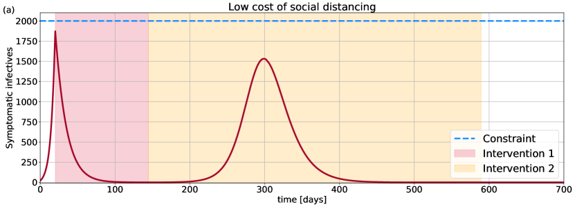
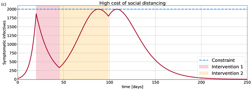
In the present example, an intervention protocol is optimised. We consider the SIIR model with two age groups, with fictitious parameters and a fictitious contact matrix. The protocol consists of two durations, namely

• the duration $T_{1}$ of a full lockdown (implemented in this toy model by reducing the initial contact matrix via a prefactor $1/4$), and

• the duration $T_{2}$ a subsequent partial lockdown (implemented in this toy model by reducing the initial contact matrix via a prefactor $3/4$).

For illustrative purposes we choose the cost function

$$\mathcal{C}=\exp\left[\kappa\left(T_{1}+\frac{T_{2}}{5}\right)\right]+\frac{1}{\tau}\int_{0}^{t_{f}}\mathrm{d}t\,I_{s}(t),$$ (1)

where $t_{f}=1000$ days is the final time of the simulation, and $I_{s}(t)$ is the total number of symptomatic infectives at time $t$. The first term in equation (1) can be thought of as a cost for social distancing, while the second terms models a cost of infection. The time scale $\tau$ determines the relative importance of the two terms, and in our example we use $\tau=1$. We additionally set $\mathcal{C}=\infty$ if at any time $I_{s}(t)>2000$, which serves as a hard constraint that every protocol must keep the number of infectives below a threshold. The rate $\kappa$ in the first term of equation (1) determines the exponential increase in cost per time during lockdown, and in the present example we minimise the total cost as a function of $(T_{1},T_{2})$, considering three distinct scenarios: i) low cost of social distancing ($\kappa=0.01/$day), ii) intermediate cost of social distancing ($\kappa=0.1/$day), and iii) high cost of social distancing ($\kappa=1/$day). Finally, we compare the time series corresponding to these optimal protocols.

⬇

import numpy as np

import matplotlib.pyplot as plt

import pyross

from multiprocessing import Pool

import cma

import time

from functools import partial

# 1. Define model

# number of age groups and total population

M = 2 # the population has two age groups

N = 5e4 # and this is the total population

# model parameters

beta = 0.02 # infection rate

gIa = 1./7 # removal rate of asymptomatic infectives

gIs = 1./7 # removal rate of asymptomatic infectives

alpha = 0.2 # fraction of asymptomatic infectives

fsa = 0.8 # the self-isolation parameter

# set the age structure

fi = np.array([0.25, 0.75]) # fraction of population in age age group

Ni = N*fi

# set up initial condition

Ia0 = np.array([10, 10]) # each age group has asymptomatic infectives

Is0 = np.array([10, 10]) # and also symptomatic infectives

R0 = np.array([0, 0]) # there are no removed individuals initially

S0 = Ni - (Ia0 + Is0 + R0) # initial number of susceptibles

# 2. Define function that generates two-step release protocol

def get_events(protocol= [50,100]):

end_phase_1, end_phase_2 = protocol

C = np.array([[18., 9.], [3., 12.]])

events = []; contactMatrices = []

# Note that the event functions take a vector argument

# "xt" instead of a tuple (S, Ia, Is).

# When defining the event functions for the SIR

# model, the following correspondence has to be used:

# S == xt[ :M]

# Ia == xt[1*M:2*M]

# Is == xt[2*M:3*M]

# (For any model, the order for the event functions is

# exactly the same as in the arguments of model.simulation)

#

# This is a dummy event which will never occur;

# it is used to set the initial contact matrix

events.append( lambda t, xt: 1. )

contactMatrices.append( C )

# Event 1: contact matrix reduced by a factor of 4 once

# number of symptomatic infectives exceeds a threshold

# ("start of full lockdown")

lockdown_threshold_on = 1900

def event1(t,xt):

return np.sum(xt[2*M:3*M]) - lockdown_threshold_on

event1.direction = +1 # need to pass threshold from below for event

events.append(event1); contactMatrices.append( 0.25*C )

# Event 2: contact matrix at 75% of original contact matrix after

# a given time ("start of partial lockdown").

def event2(t,xt):

return t - end_phase_1

events.append(event2); contactMatrices.append( 0.75*C )

# Event 3: original contact matrix is restored after a given time

# ("end of partial lockdown").

def event3(t,xt):

return t - end_phase_2

events.append(event3); contactMatrices.append( C )

return events, contactMatrices

# 3. Define cost function

maximal_value_for_Is = 2000

def evaluate_cost_function(t_arr,traj,protocol,events_occured,

sdc_prefactor=1.,

sdc_rate=1/7.):

infinity = 1e300 # using np.inf would be more proper, but will

# result in warnings throughout the minimization once a protocol

# is probed that violates one of the hard constraints.

#

# hard constraints:

# - times of protocol need to be non-negative

if (np.array(protocol) < 0).any(): return infinity

# - second stage of intervention needs to end after first stage ends

if protocol[0] > protocol[1]: return infinity

# - second stage of intervention needs to end before 700 days

if protocol[1] > 700: return infinity

# - number of symptomatic infectives should

# never exceed a given maximal value

if np.max( np.sum( traj[2*M:3*M],axis=0 ) ) > maximal_value_for_Is:

return infinity

# Evaluate results of protocol.

# Which phases have occured in the simulation?

have_lockdown_start = False

have_lockdown_end_0 = False

have_lockdown_end_1 = False

for i,e in enumerate(events_occured):

if e[1] == 1:

lockdown_start = e[0]

have_lockdown_start = True

elif e[1] == 2:

lockdown_end_0 = e[0]

have_lockdown_end_0 = True

elif e[1] == 3:

lockdown_end_1 = e[0]

have_lockdown_end_1 = True

# calculate cost function

cost = 0.

# cost of social distancing

if have_lockdown_start:

if have_lockdown_end_0:

cost += sdc_prefactor* np.exp(sdc_rate* \

(lockdown_end_0-lockdown_start))

else:

cost += infinity

#

if have_lockdown_end_0 and have_lockdown_end_1:

cost *= np.exp(0.2*sdc_rate*(lockdown_end_1-lockdown_end_0))

# cost of infection

cost += np.trapz( np.sum( traj[2*M:3*M],axis= 0 ),t_arr)

return cost

# 4. Define function that evaluates the cost of a given protocol

def evaluate_cost_of_protocol(model,protocol,

verbose=False,return_trajectory=False,

sdc_prefactor=10.,

sdc_rate=1/7.):

# define events corresponding to given protocol

events, contactMatrices = get_events(protocol)

# run simulation

Tf = 1000; Nt = (Tf +1)*10

result = model.simulate(S0, Ia0, Is0,

events=events,contactMatrices=contactMatrices,

Tf=Tf, Nf=Nt)

# evaluate cost

cost = evaluate_cost_function(t_arr=result[’t’],

traj=result[’X’].T,

protocol=protocol,

events_occured=result[’events_occured’],

sdc_prefactor=sdc_prefactor,

sdc_rate=sdc_rate)

if return_trajectory:

return cost, result[’t’], result[’X’], result[’events_occured’]

else:

return cost

# 5. Define minimiser

def minimizing_function(sdc_prefactor,sdc_rate,

protocol):

#This is the function that will be minimised by the cma-es algorithm

costs = evaluate_cost_of_protocol(model=model,

protocol=protocol,

sdc_prefactor=sdc_prefactor,

sdc_rate=sdc_rate,

return_trajectory=False)

return costs

def find_optimal_protocol(initial_guess,sdc_prefactor,sdc_rate,

model,

verbose=True,initial_variance=5.):

func = partial(minimizing_function, sdc_prefactor, sdc_rate)

# set parameters for minimisation based on cma-es algorithm

number_of_threads = 4

number_iterations = 1000

p = Pool(number_of_threads)

options = cma.CMAOptions()

options[’popsize’] = 12

# run minimisation

start_time = time.time()

optim = cma.CMAEvolutionStrategy(initial_guess, initial_variance,

options)

iteration = 0

while not optim.stop() and iteration < number_iterations:

positions = optim.ask()

values = p.map(func, positions)

optim.tell(positions, values)

optim.disp()

iteration += 1

end_time = time.time()

if verbose:

print("Time: ", end_time - start_time)

print("Value: ", optim.best.f)

print("Parameters: ",optim.best.x)

return optim.best.x

# 6. Find optimal protocol for three different scenarios

# Initialise model

parameters = {’alpha’:alpha,’beta’:beta, ’gIa’:gIa,’gIs’:gIs,’fsa’:fsa}

model = pyross.control.SIR(parameters, M, Ni)

initial_guess=[70,200] # use same initial guess for all minimisations

sdc_prefactor = 1. # means that social distancing cost and

# cost of infection have the same weight in our model

# Low, intermediate, and high cost rate for social distancing:

sdc_rates = [1e-2,1e-1,1.]

optimal_protocols = []

for i,sdc_rate in enumerate(sdc_rates):

optimal_protocol = find_optimal_protocol(initial_guess=initial_guess,

sdc_prefactor=sdc_prefactor,

sdc_rate=sdc_rate,

model=model)

optimal_protocols.append(optimal_protocol)

# 7. Visualise results

def plot_result(protocol,model,

title=’Optimised intervention parameters’,

t_max=None):

#

cost, t_arr, traj, events_occured = evaluate_cost_of_protocol(

model=model,

protocol=protocol,

return_trajectory=True)

Is = np.sum(traj[:,2*M:],axis=-1)

fig, ax = plt.subplots(1,1,figsize=(7,5))

ax.set_title(title)

ax.axhline(maximal_value_for_Is,color=’red’,ls=’--’,

label=r’Constraint’)

ax.axvspan(events_occured[0][0],events_occured[1][0],

color=’crimson’,label=’Intervention 1’,alpha=0.2)

ax.axvspan(events_occured[1][0],events_occured[2][0],

color=’orange’,label=’Intervention 2’,alpha=0.2)

ax.plot(t_arr,Is)

if t_max == None:

ax.set_xlim(np.min(t_arr),np.max(t_arr))

else:

ax.set_xlim(np.min(t_arr),t_max)

ax.set_ylabel(’Symptomatic infectives’)

ax.set_xlabel(r’time [days]’)

ax.legend(loc=’upper right’,fontsize=12,framealpha=1.)

plt.show(); plt.close(fig)

optimal_protocol_labels = [’Low cost of social distancing’,

’Intermediate cost of social distancing’,

’High cost of social distancing’]

t_max = [700,250,250]

for i,optimal_protocol in enumerate(optimal_protocols):

plot_result(protocol=optimal_protocol,model=model,t_max=t_max[i],

title=optimal_protocol_labels[i])

Figure 1: Optimisation of NPI protocol parameters, c.f. example 7. The protocol consists of two durations, namely the time of a full lockdown (initial contact matrix reduced via a prefactor 1/4), and a subsequent partial lockdown (initial contact matrix reduced via a prefactor 3/4). The cost of a protocol is comprised of a i) cost for social distancing (= reducing the entries of the contact matrix), and ii) a cost of infection. As a hard constraint, the protocol must keep the number of infectives below a defined threshold, shown as horizontal dashed line. The optimal protocol minimises the total cost. Subplots (a), (b), (c), show three results of optimisation for the same system, depending on the cost of social distancing.

8 Model sensitivity

Here we illustrate the usage of PyRoss to study model sensitivity. We use four different models, SIR, SEIR, SIR with stages, and SEIR with stages. The models predict similar epidemic curve before the lockdown, while the they show distinct behavior after lockdown. We show that the addition of an exposed $E_{i}$ compartment (to give an age-structured SEIR model) makes the infectious number grows beyond the lockdown for the time scale of the incubation. Note that while this example employs UK age groups and contact structure, the model parameters are not fitted to real epidemiological data.

⬇

import numpy as np

import pyross

import matplotlib.pyplot as plt

## population and age classes

M=16 ## number of age classes

my_data = np.genfromtxt(’India-2019.csv’, delimiter=’,’, skip_header=1)

Ni = (my_data[:, 1]+ my_data[:, 2])[0:M]

# Get individual contact matrices

CH, CW, CS, CO = pyross.contactMatrix.India()

# Generate contact matrix

generator = pyross.contactMatrix.ContactMatrixFunction(CH, CW, CS, CO)

Tf=42; Nf=600

times= [21, Tf] # temporal boundaries between different contact-behaviour

aW, aS, aO = 0.0, 0.0, 0.0

# prefactors for CW, CS, CO:

interventions = [[1.0,1.0,1.0], # before first time

[aW, aS, aO], # between first and second time

]

# generate corresponding contact matrix function

contactMatrix = generator.interventions_temporal(times=times,interventions=interventions)

# ## SIR

beta = 0.01646692 # probability of infection on contact

gIa = 1./7 # removal rate of asymptomatic infectives

gIs = 1./7 # removal rate of symptomatic infectives

alpha = 0. # asymptomatic fraction

fsa = 1 # suppresion of contact by symptomatics

# initial conditions

Is_0 = np.zeros((M)); Is_0[6:13]=14; Is_0[2:6]=13

Ia_0 = np.zeros((M))

R_0 = np.zeros((M))

S_0 = Ni - (Ia_0 + Is_0 + R_0)

parameters = {’alpha’:alpha,’beta’:beta, ’gIa’:gIa,’gIs’:gIs,’fsa’:fsa}

model = pyross.deterministic.SIR(parameters, M, Ni)

dataSIR =model.simulate(S_0, Ia_0, Is_0, contactMatrix, Tf, Nf)

I1 = model.Is(dataSIR)

# ## SEIR

beta = 0.027 # probability of infection on contact

gIa = 1./7 # removal rate of asymptomatic infectives

gE = 1/2.72 # removal rate of exposeds

gIs = 1./7 # removal rate of symptomatic infectives

alpha = 0. # asymptomatic fraction

fsa = 1 # suppresion of contact by symptomatics

Is_0 = np.zeros((M)); Is_0[6:13]=14; Is_0[2:6]=13

Ia_0 = np.zeros((M))

E_0 = np.zeros((M));

R_0 = np.zeros((M))

S_0 = Ni - (Ia_0 + Is_0 + R_0)

param={’alpha’:alpha,’beta’:beta,’gIa’:gIa,’gIs’:gIs,’gE’:gE,’fsa’:fsa}

model = pyross.deterministic.SEIR(param, M, Ni)

dataSEIR =model.simulate(S_0, E_0, Ia_0, Is_0, contactMatrix, Tf, Nf)

I2 = model.Is(dataSEIR)

# SIR with stages (SIkR)

beta = 0.01324 # probability of infection on contact

gI = 1./7 # removal rate of infectives

gE = 1/2.72 # removal rate of exposeds

kI = 32; # # of stages of I class

I0 = np.zeros((kI,M));

for i in range(kI):

I0[i, 6:13]=14; I0[i, 2:6]=13

S0 = np.zeros(M)

for i in range(M) :

S0[i] = Ni[i] - np.sum(I0[:,i])

I0 = np.reshape(I0, kI*M)/kI

parameters = {’beta’:beta, ’gI’:gI, ’kI’:kI}

model = pyross.deterministic.SIkR(parameters, M, Ni)

dataSIkR=model.simulate(S0, I0, contactMatrix, Tf, Nf)

I3 = model.I(dataSIkR)

# SEIR with stages (SEkIkR)

beta = 0.0188 # probability of infection on contact

gI = 1./7 # removal rate of infectives

gE = 1/2.72 # removal rate of exposeds

kI = 32; # # of stages of I class

kE = 2; # # of stages of E class

S0 = np.zeros(M)

I0 = np.zeros((kI,M));

E0 = np.zeros((kE,M));

for i in range(kI):

I0[i, 6:13]=14; I0[i, 2:6]=13

for i in range(kE):

E0[i, 0:16]=14

for i in range(M) :

S0[i] = Ni[i] - np.sum(I0[:,i]) - np.sum(E0[:,i])

I0 = np.reshape(I0, kI*M)/kI;

E0 = np.reshape(E0, kE*M)/kE;

parameters = {’beta’:beta, ’gE’:gE, ’gI’:gI, ’kI’:kI, ’kE’ : kE}

model = pyross.deterministic.SEkIkR(parameters, M, Ni)

data=model.simulate(S0,E0,I0,contactMatrix,Tf,Nf); I4 = model.I(data)

asI1,asI2,asI3,asI4 = I1.sum(axis=1),I2.sum(axis=1),I3.sum(axis=1),I4.sum(axis=1) #sum over all ages

plt.plot(t, asI1, ’-’, lw=lwd, color=’#A60628’, label=’SIR’)

plt.plot(t, asI3, ’-’, lw=lwd, color=’#348ABD’, label=’SIkR’)

plt.plot(t, asI2, ’-’, lw=lwd, color=’goldenrod’, label=’SEIR’)

plt.plot(t, asI4, ’-’, lw=lwd, color=’forestgreen’, label=’SEkIkR’)

plt.xlabel(’Days’); plt.ylabel(’Infected individuals’);

Figure 1: Model-dependence of dynamics after lockdown. In example 8, the models SIR, SEIR, SIR with stages, and SEIR with stages, are considered. Parameters are chosen such that the initial grow rates are comparable. Initially, all models use the full contact matrix, which is the sum of home, work, school, and other contacts. At a fixed time, a lockdown is modeled by retaining only the home contacts. This plot illustrates the resulting different model dynamics at the initial phase of the lockdown.

Chapter 5 Conclusion

This report has presented an overview of PyRoss, a Python library that integrates compartment models of epidemics with Bayesian inference and optimization tools.

The current focus of PyRoss, and hence of this report, is on well-mixed, age-structured models with a modest number of contact channels (home, school, workplace, other). However, PyRoss allows these channels to be expanded indefinitely in principle, so that more complex contact information relating to particular working or social environments can be incorporated as available.

Likewise PyRoss allows the disease stages themselves to be subdivided at will. This enables the statistics of objective medical states, such as hospitalization and intensive care or ventilator use, to be modelled. By also allowing an indefinitely expandable number of compartments per disease stage, the residence time distribution in such stages can be varied from the exponential decay of simple compartment models to the sharply-peaked distribution that underlies time-since-infection models [10, 11, 12, 13, 14, 15]. Certain other mathematical limitations can be overcome similarly.

NPIs are viewed within PyRoss as strategies to influence contact matrices, generally in a time-dependent fashion, through variations in contact rate, or transmission rate at contact, or both. These interventions can be represented in as much social detail as is resolved by the contact matrices themselves.

A Bayesian system of inference for model parameters, and for forecasting with error estimation, is fully integrated into PyRoss. The former is a crucial feature which allows comparison between models based on evidence. This can guide a principled expansion in the number of compartments up to a level of granularity justified by the data, and can warn when this has gone too far. The approach guards against over-fitting of historic data, leading to precise but inaccurate forecasting – a risk faced by parameter-rich, data-poor models in any field of science.

One can expect robust inference from historic data to prove crucial for forecasting the future course of an epidemic, particularly where sequenced or nuanced NPIs are involved. Accordingly, PyRoss’s Bayesian parameter estimation tools allow the fitting of time-dependent contact-matrix parameters representing NPIs. Prior estimates (supplied perhaps by expert judgement) of the effect of an NPI on contact statistics can therefore be continuously improved, after the NPI is implemented, by feeding the observed results back into the system (Fig. 1). Observed outcomes for one NPI (such as sudden lockdown) can inform the prediction of others (such as a sequential, age-stratified unlock).

Within PyRoss, given a user-defined cost function that encodes their harm, NPIs can be optimized and ranked by minimization of the chosen cost function. The actual choice of cost functions is, of course, morally and politically problematic. However, there are many other areas of planning where saving life is weighed against economic cost, including decisions about where and whether to build a new hospital, or indeed a new road.

The principles of compartment modelling embraced by PyRoss, when constrained by a disciplined approach to parameter and uncertainty estimation, are, we believe, more powerful than is widely assumed, but of course not all-powerful. Known challenges include situations in which the well-mixed approximation does not hold at small scales, such as the fact that isolation by household can allow rapid disease spread within each household while preventing it at societal level. Redesign of the compartment structure to reflect a different ‘unit of infection’, such as a household, may help in some such cases.

In contrast, there is no problem of principle in extending compartment models to societies that are locally well mixed but heterogeneous at larger scales. Different contact matrices can be assigned at regional level and/or to micro-locations such as specific workplaces or social venues. Once such geo-social compartments are resolved, the transition rates between them are controlled by human mobility which can itself be modelled by jumps into and out of compartments representing journeys (within which infection can of course occur). NPIs can then separately target either the locationally specific contact matrices, or the transfer of people between locations. In a forthcoming report we will describe PyRossGeo, an extension of PyRoss along these lines.

This report has focussed on the design principles and capabilities of PyRoss, illustrated by very simple examples of its use. We have not deployed it directly here to address aspects of the current COVID-19 crisis, but for an example of its use in doing so, see [16]. (Note that since that paper was written, the capabilities of PyRoss have advanced dramatically.)

The PyRoss library is open-source. We positively encourage its use by other scientists, whether seasoned epidemic modellers or those new to the field. We hope it can contribute to a stronger scientific platform for evidence-based decision making as the current pandemic continues, and also before the next one.

Acknowledgement

The work described in this report was completed in the six weeks spanning April to mid-May 2020 as a contribution to the Rapid Assistance in Modelling the Pandemic (RAMP) initiative, coordinated by the Royal Society. The GitLab platform enabled seamless collaboration under lockdown conditions. We are grateful to the numerous developers who contribute to the open-source platform on which PyRoss is built and without which it would not exist. We acknowledge advice from Graeme Ackland, Daan Frenkel, Julia Gog, Chris Rogers, and Richard Wilkinson. We thank the code review team of RAMP’s Rapid Review Group at Oxford for their scrutiny of the PyRoss library and for their suggestions for improvement; RAMP’s Red Team at Edinburgh further code review and stress testing; and those who opened issues and offered suggestions on GitHub. Remaining defects in the PyRoss library and in this report are the responsibility of the authors. This work was funded in part by the European Research Council under the EU’s Horizon 2020 Program, Grant No. 740269; by the Royal Society through a Research Professorship held by MEC, and by an Early Career Grant to RA from the Isaac Newton Trust.

Appendix: Simple versus Complicated Models

Figure 1: Predictions from an unstructured SI5R model in Simulana. Simulana is an imagined country where epidemics are correctly described by the Covid-Sim algorithm of [19] with some particular parameter set.

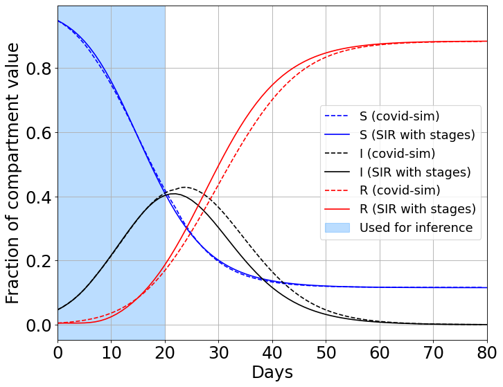
Let us imagine an alternative universe which contains a country resembling the UK, called Simulana, for which the CovidSim model, with a specific parameter set as selected in [19], describes the disease dynamics as well as one could wish. The government of Simulana allow the epidemic to run its course without NPIs. Suppose that the only data available to modellers in Simulana are time-resolved national aggregate statistics $(S(t),I(t),R(t))$ for the number of susceptibles, infecteds, and removeds. To forecast the epidemic, the modellers adopt an age-unstructured SIkR model, with $k$, the number of infected sub-compartments discussed above, set to $k=5$. We emphasise that this is an utterly basic model. Nonetheless, by fitting to the available data up to (say) the point where $S=I$, Simulana’s modellers are able to predict its remaining course reasonably well, as shown in Figure 1. Note that only the maximum a posteriori (MAP) prediction is shown although PyRoss can deliver the full posterior distribution if required.

These predictions raise the following question: Unless the specific CovidSim parameters that correctly describe epidemics in Simulana are disclosed upfront by revelation, is CovidSim in general much better at predicting epidemics there than, say, SI5R?

Interpreting this question in a strictly Bayesian sense of ‘which model has more evidence’, we suspect the answer is ‘no’ – although to confirm this quantitatively would require a more precise delineation of CovidSim’s free parameters than we currently have. This is because the Bayesian ‘Occam factors’ penalize models with parameters that are unconstrained by the data available: the evidence for these models is small, whereas parsimonious models always have larger evidence if equally capable of fitting the data.

But even if the question is interpreted less formally, we might also suspect a negative answer. Given the limited medical data available in Simulana, it is not clear that this can constrain CovidSim’s parameters sufficiently to give forecasts that are any more reliable than those of much simpler models. This is despite the fact that using CovidSim the epidemic in Simulana’s could be forecast perfectly in principle if the correct parameters were known.

In the above example, the modellers of Simulana received only aggregate patient data; alternatively they might receive data stratified by age, geography etc.. In this case the shortcomings of SI5R for Simulana would soon be revealed by the Bayesian approach. However, a generalized compartment model might well still beat CovidSim at ‘predicting its own future’. Of particular promise are models whose compartments broadly aligned with the granularity of the data available, creating inbuilt parsimony.

It is very important to recognize that the above paragraphs contain no specific criticism of CovidSim itself, or any other particular model. Instead they express a more general concern about basing predictions on any model whose parameters have proliferated beyond the ability of data to estimate them. Such concerns apply not only for epidemics but across many other disciplines. They are one of the reasons so many scientists today prefer a Bayesian approach to model and parameter selection, as offered by PyRoss for compartment models.

References

- [1] R. M. Anderson, B. Anderson, and R. M. May. Infectious diseases of humans: dynamics and control. Oxford university press, 1992.
- [2] M. J. Keeling and P. Rohani. Modeling infectious diseases in humans and animals. Princeton University Press, 2011.
- [3] N. T. J. Bailey. The mathematical theory of infectious diseases and its applications. Charles Griffin & Company Ltd, 5a Crendon Street, High Wycombe, Bucks HP13 6LE., 1975.
- [4] D. Anderson and R. Watson. On the spread of a disease with gamma distributed latent and infectious periods. Biometrika, 67(1):191–198, 1980.
- [5] H. J. Wearing, P. Rohani, and M. J. Keeling. Appropriate models for the management of infectious diseases. PLoS medicine, 2(7), 2005.
- [6] O. Krylova and D. J. D. Earn. Effects of the infectious period distribution on predicted transitions in childhood disease dynamics. Journal of The Royal Society Interface, 10(84):20130098, 2013.
- [7] A. L. Lloyd. Realistic distributions of infectious periods in epidemic models: changing patterns of persistence and dynamics. Theoretical population biology, 60(1):59–71, 2001.
- [8] H. Barbosa, M. Barthelemy, G. Ghoshal, et al. Human mobility: Models and applications. Physics Reports, 734:1–74, 2018.
- [9] S. M. Jenness, S. M. Goodreau, and M. Morris. Epimodel: an r package for mathematical modeling of infectious disease over networks. Journal of statistical software, 84, 2018.
- [10] W. O. Kermack and A. G. McKendrick. A contribution to the mathematical theory of epidemics. Proceedings of the royal society of london. Series A, Containing papers of a mathematical and physical character, 115(772):700–721, 1927.
- [11] J. Reddingius. Notes on the mathematical theory of epidemics. Acta biotheoretica, 20(3-4):125–157, 1971.
- [12] L. Sattenspiel, K. Dietz, et al. A structured epidemic model incorporating geographic mobility among regions. Mathematical biosciences, 128(1):71–92, 1995.
- [13] F. Hoppensteadt. An age dependent epidemic model. Journal of the Franklin Institute, 297(5):325–333, 1974.
- [14] O. Diekmann, J. A. P. Heesterbeek, and M. G. Roberts. The construction of next-generation matrices for compartmental epidemic models. J. Royal Soc. Int., 7(47):873–885, 2010.
- [15] H. R. Thieme and C. Castillo-Chavez. How may infection-age-dependent infectivity affect the dynamics of HIV/AIDS? SIAM Journal on Applied Mathematics, 53(5):1447–1479, 1993.
- [16] Rajesh Singh and R Adhikari. Age-structured impact of social distancing on the covid-19 epidemic in india. arXiv preprint arXiv:2003.12055, 2020.
- [17] D. J. C. MacKay. Information theory, inference and learning algorithms. Cambridge University Press, 2003.
- [18] D. J. C. MacKay. Bayesian interpolation. Neural computation, 4(3):415–447, 1992.
- [19] N. M. Ferguson et al. Impact of non-pharmaceutical interventions (npis) to reduce covid-19 mortality and healthcare demand. London: Imperial College COVID-19 Response Team, March, 16, 2020.
- [20] S. Towers and Z. Feng. Social contact patterns and control strategies for influenza in the elderly. Math. Biosci., 240(2):241–249, 2012.
- [21] N. M. Ferguson et al. Strategies for mitigating an influenza pandemic. Nature, 442(7101):448–452, 2006.
- [22] H. W. Hethcote. The mathematics of infectious diseases. SIAM review, 42(4):599–653, 2000.
- [23] J. Glasser, Z. Feng, A. Moylan, S. Del Valle, and C. Castillo-Chavez. Mixing in age-structured population models of infectious diseases. Mathematical Biosciences, 235(1):1–7, 2012.
- [24] K. Prem, A. R. Cook, and M. Jit. Projecting social contact matrices in 152 countries using contact surveys and demographic data. PLoS Comp. Bio, 13(9):e1005697, 2017.
- [25] R. Ross. An application of the theory of probabilities to the study of a priori pathometry. Proceedings of the Royal Society of London, 92(638):204–230, 1916.
- [26] S. Busenberg and C. Castillo-Chavez. A general solution of the problem of mixing of subpopulations and its application to risk-and age-structured epidemic models for the spread of aids. Mathematical Medicine and Biology: A Journal of the IMA, 8(1):1–29, 1991.
- [27] J. Wallinga, Peter T., and M. Kretzschmar. Using data on social contacts to estimate age-specific transmission parameters for respiratory-spread infectious agents. American journal of epidemiology, 164(10):936–944, 2006.
- [28] R. F. Pawula. Approximation of the linear boltzmann equation by the fokker-planck equation. Phys. Rev., 162:186–188, Oct 1967.
- [29] C. W. Gardiner. Handbook of stochastic methods. Springer Berlin, 1985.
- [30] N. G. Van Kampen. Stochastic processes in physics and chemistry, volume 1. Elsevier, 1992.
- [31] M. Komorowski, B. Finkenstaedt, C. V Harper, and D. A Rand. Bayesian inference of biochemical kinetic parameters using the linear noise expansion. BMC Bioinformatics, 10(343), 2009.
- [32] R. Singh, D. Ghosh, and R. Adhikari. Fast bayesian inference of the multivariate ornstein-uhlenbeck process. Phys. Rev. E, 98:012136, Jul 2018.
- [33] D. Maclaurin, D. Duvenaud, and R. P. Adams. Autograd: Effortless gradients in numpy. In ICML 2015 AutoML Workshop, volume 238, 2015.
- [34] https://github.com/kbarbary/nestle.
- [35] J. Skilling. Nested sampling for general bayesian computation. Bayesian analysis, 1(4):833–859, 2006.
- [36] James Bradbury, Roy Frostig, Peter Hawkins, Matthew James Johnson, Chris Leary, Dougal Maclaurin, and Skye Wanderman-Milne. JAX: composable transformations of Python+NumPy programs, 2018.
- [37] D. T. Gillespie. Exact stochastic simulation of coupled chemical reactions. The Journal of Physical Chemistry, 81(25):2340–2361, December 1977.
- [38] D. T. Gillespie. Approximate accelerated stochastic simulation of chemically reacting systems. The Journal of Chemical Physics, 115(4):1716–1733, July 2001.
- [39] Y. Cao, D. T. Gillespie, and L. R. Petzold. Efficient step size selection for the tau-leaping simulation method. The Journal of Chemical Physics, 124(4):044109, January 2006.
- [40] G. Wanner and E. Hairer. Solving ordinary differential equations II: Stiff and differential-algebraic problems. Springer Berlin Heidelberg, 1996.
- [41] E. Hairer, S. P Nørsett, and G. Wanner. Solving ordinary differential equations I: Nonstiff problems, 1993.
- [42] H. P. Langtangen and L. Wang. Odespy. https://github.com/hplgit/odespy, 2014.
- [43] P. Virtanen, R. Gommers, T. E. Oliphant, et al. Scipy 1.0: fundamental algorithms for scientific computing in python. Nature methods, 17(3):261–272, 2020.
- [44] https://www.populationpyramid.net/.
- [45] Z. Feng and H. R. Thieme. Endemic models with arbitrarily distributed periods of infection i: Fundamental properties of the model. SIAM Journal on Applied Mathematics, 61(3):803–833, 2000.
- [46] R. Pastor-Satorras, C. Castellano, P. Van Mieghem, and A. Vespignani. Epidemic processes in complex networks. Reviews of modern physics, 87(3):925, 2015.
- [47] M. Y. Li and J. S Muldowney. Global stability for the seir model in epidemiology. Mathematical biosciences, 125(2):155–164, 1995.
- [48] J. A. P. Heesterbeek. A brief history of and a recipe for its calculation. Acta biotheoretica, 50(3):189–204, 2002.
- [49] S. Townley, D. Carslake, O. Kellie-Smith, D. Mccarthy, and D. Hodgson. Predicting transient amplification in perturbed ecological systems. Journal of Applied Ecology, 44(6):1243–1251, 2007.
- [50] I. Stott, D. J. Hodgson, and S. Townley. Beyond sensitivity: Nonlinear perturbation analysis of transient dynamics. Methods in Ecology and Evolution, 3(4):673–684, 2012.
- [51] M. Asllani, R. Lambiotte, and T. Carletti. Structure and dynamical behavior of non-normal networks. Science Advances, 4(12):1–9, 2018.
- [52] M. Asllani and T. Carletti. Topological resilience in non-normal networked systems. Physical Review E, 97(4):1–12, 2018.
- [53] L. N. Trefethen and M. Embree. Spectra and pseudospectra: the behavior of nonnormal matrices and operators. Princeton University Press, 2005.