∎
Learning Equations from Biological Data with Limited Time Samples††thanks: This material was based upon work partially supported by the National Science Foundation under Grant DMS-1638521 to the Statistical and Applied Mathematical Sciences Institute and IOS-1838314 to KBF, and in part by National Institute of Aging grant R21AG059099 to KBF. Any opinions, findings, and conclusions or recommendations expressed in this material are those of the authors and do not necessarily reflect the views of the National Science Foundation. BM gratefully acknowledges PhD studentship funding from the UK EPSRC (reference EP/N50970X/1). AHD, LC, and KRS gratefully acknowledge funding through the NIH U01CA220378 and the James S. McDonnell Foundation 220020264.
Abstract
Equation learning methods present a promising tool to aid scientists in the modeling process for biological data. Previous equation learning studies have demonstrated that these methods can infer models from rich datasets, however, the performance of these methods in the presence of common challenges from biological data has not been thoroughly explored. We present an equation learning methodology comprised of data denoising, equation learning, model selection and post-processing steps that infers a dynamical systems model from noisy spatiotemporal data. The performance of this methodology is thoroughly investigated in the face of several common challenges presented by biological data, namely, sparse data sampling, large noise levels, and heterogeneity between datasets. We find that this methodology can accurately infer the correct underlying equation and predict unobserved system dynamics from a small number of time samples when the data is sampled over a time interval exhibiting both linear and nonlinear dynamics. Our findings suggest that equation learning methods can be used for model discovery and selection in many areas of biology when an informative dataset is used. We focus on glioblastoma multiforme modeling as a case study in this work to highlight how these results are informative for data-driven modeling-based tumor invasion predictions.
Keywords:
Equation learning numerical differentiation sparse regression model selection partial differential equations parameter estimation population dynamics glioblastoma multiforme1 Introduction
Mathematical models are a crucial tool for inferring the mechanics underlying a scientific system of study nardini_modeling_2016 or predicting future outcomes ferguson_NPIs_2020 . The task of interpreting biological data in particular benefits from mathematical modeling, as models allow biologists to test multiple hypotheses in silico ozik_high-throughput_2018 , optimally design experiments walter_qualitative_1990 , or create personalized medical treatment plans for patients baldock_patient-specific_2014 . A common question for mathematicians and biologists alike is: which model(s) sufficiently describe a given data set warne_using_2019 ? This is a challenging question to resolve, as there may be several candidate models that can describe the data comparably well, or the underlying mechanics may be poorly understood. This challenge of inferring a data-driven mathematical model is further complicated by common issues with biological data that inhibit our understanding of the underlying dynamics. Such challenges include large amounts of noise francis_quantifying_2003 ; perretti_model-free_2013 , sparse time sampling baldock_patient-specific_2014 ; massey_image-based_2020 ; hawkins-daarud_quantifying_2019 , inter-population heterogeneity wang_prognostic_2009 , and complex forms of observation noise banks2014modeling ; lagergren_learning_2020
Partial differential equations (PDEs) are used to model many spatiotemporal phenomena, ranging from the signaling proteins inside of cells mori_wave-pinning_2008 to the migration patterns of animal populations garcia-ramos_evolutionary_2002 . Reaction-diffusion-advection equations in particular are suited to describe biological processes that involve the simultaneous transport and growth or decay of a substance over time. Such equations may be written as
| (1) |
with system-specific initial and boundary conditions for some quantity of interest that spreads with diffusion rate , migrates with advection rate , and grows or decays with reaction rate . One common example used for modeling biological phenomena is the Fisher-Kolmogorov-Petrovsky-Piskunov (Fisher-KPP) equation fisher_wave_1937 :
| (2) |
This equation assumes has a constant rate of diffusion , grows logistically with intrinsic growth rate until it reaches the population carrying capacity , and does not advect (). Given an initial condition with compact support, solutions to the Fisher-KPP equation converge to traveling wave solutions that spread with constant speed kolmogoroff_etude_1937 . One can also show that the steepness of the propagating front depends on the ratio ; the front becomes more steep as decreases and becomes more spread out as increases, see murray_mathematical_2002 for details.
The Fisher-KPP Equation was initially proposed to model the spread of an advantageous gene fisher_wave_1937 , but has since been used to model many biological phenomena including wound healing experiments jin_reproducibility_2016 ; nardini_investigation_2018 ; warne_using_2019 and the spread of invasive species urban_toad_2008 . In particular, it has been shown to be an informative model for glioblastoma multiforme (GBM), an aggressive brain tumor known for its heterogeneous behavior between patients baldock_patient-specific_2014 ; massey_image-based_2020 ; rockne_patient-specific_2015 . Using two time samples of standard clinical imaging in conjunction with key assumptions about how the imaging relates to cell density, the parameters and can be estimated for patients based on the wave front velocity and steepness hawkins-daarud_quantifying_2019 . Inferring these two parameters from patient data aids in characterizing the inter-patient heterogeneity common to this disease, thereby enabling data-driven modeling-based prognosis. For example, Baldock et al. baldock_patient-specific_2014 found that a patient-specific metric of invasiveness, given by , predicts the survival benefit of gross total resection for GBM patients and, more recently, Massey et al. massey_image-based_2020 correlated this metric with temozolomide efficacy, a chemotherapy drug currently used in the standard of care to treat GBM. The accurate selection of a mathematical model to aid in interpreting patient GBM data is a vital tool in informing our understanding of the efficacy of potential treatment plans for this disease.
The Fisher-KPP Equation thus serves as a useful model that provides insight into patient GBM dynamics through model prognosis and prediction of outcomes from therapeutic interventions massey_image-based_2020 . For any scientific process (GBM progression, population growth, species migration, etc.), determining which model accurately describes the underlying dynamics can be a challenging process. Common methods to choose such a model include deriving a multi-scale model from assumptions on individual interactions nardini_modeling_2016 , theorizing a heuristic model from expert knowledge, or utilizing model selection techniques bortz_model_2006 ; ulmer_topological_2019 ; warne_using_2019 . Model selection studies often consider several plausible hypotheses to describe a given process akaike_information_1998 ; bortz_model_2006 . Whichever of these prescribed models most parsimoniously describes the data is ultimately classified as the final selected model burnham_model_2002 . Common criteria to select models include the Akaike Information Criterion (AIC) or the Bayesian Information Criterion akaike_new_1974 ; schwarz_estimating_1978 . If one has little understanding of the underlying dynamics, however, then performing a thorough model selection study may be challenging. For example, determining the form of Equation (1) that best describes a given data set can become a computationally infeasible problem due to the many possible combinations of , and that one may need to consider. Furthermore, separate numerical methods may be needed for the accurate simulation of these different term combinations, and determining the effects of numerical error on statistical inference is an ongoing area of research nardini_influence_2019 . A robust methodology to directly infer one or a few candidate models for a given biological data set will be a valuable tool for mathematical modelers.
Equation learning is a recent area of research utilizing methods from machine learning to infer the mathematical model underlying a given data set brunton_discovering_2016 ; kaiser2018sparse ; lagergren_learning_2020 ; mangan2017model ; rudy_data-driven_2017 ; zhang2018robust ; zhang_robust_2019 . Brunton et al. introduced the Sparse Identification of Nonlinear Dynamics (SINDy) algorithm, which is able to discover the governing equations underlying the chaotic Lorenz system and other systems that can be described with ordinary differential equation models brunton_discovering_2016 . This method was extended for application to PDEs in an algorithm called PDE Functional Identification of Nonlinear Dynamics (PDE-FIND) rudy_data-driven_2017 . These studies have motivated many more investigations into how modelers can infer the governing equations for experimental data, such as how methods from Bayesian inference can be used for uncertainty quantification zhang2018robust . Lagergren et al. recently demonstrated that a neural network can be used to reduce noise in data, which in turn improves the performance of the PDE-FIND algorithm in identifying biological transport models lagergren_learning_2020 . For example, the Lagergren et al. study found that the Fisher-KPP equation can be correctly inferred from spatiotemporal data that has been corrupted with proportional error with noise levels as high as 25%.
Biological data presents many challenges for equation learning methods. Equation learning studies have not been thoroughly tested in settings where data observation is limited to a small number of time samples. As many as time samples of a spatial process were observed in inferring PDE models in lagergren_learning_2020 , and the authors of rudy_data-driven_2017 considered spatiotenporal data sets with as many as 501 time samples. Rudy et al. rudy_data-driven_2017 demonstrated that the PDE-FIND algorithm can reliably infer model equations when only a small number of randomly-chosen spatial values are used for equation inference, but a dense number of spatiotemporal time samples were used prior to this inference step to estimate derivatives from the data. As the sampling of biological data is often sparse, equation learning methods must be robust in inferring equations with only limited time samples before they can be widely adopted for biological data. Furthermore, many biological phenomena exhibit wide variation between realizations. To the best of our knowledge, all previous equation learning studies infer the underlying model for only a single parameter realization without considering how the final inferred equation results change over a realistic range of parameter values. Determining how equation learning methods perform in the presence of each of these data challenges is critical if equation learning methods are to become widely adopted in the biological sciences. Such an investigation is particularly relevant for biomedical applications, including GBM growth, as clinicians may only measure the tumor volume with MR images once or twice baldock_patient-specific_2014 , and the estimated parameters for the same reaction diffusion model can vary widely between patients wang_prognostic_2009 .
We investigate two biological questions in this work: (i) how many time samples are sufficient to learn the governing equation underlying a set of data and (ii) how do these results depend on the underlying parameter values and noise levels? Such questions are of direct interest to the biological community, as data may be expensive to collect, or model parameters may not be identifiable with the available data rutter2017mathematical . Obtaining MR images in oncology, for example, can be expensive, leading to only a small number of images for each patient. This challenge leaves GBM modelers with only one or two MR images from which they can estimate patient-specific values, including the metric of invasiveness () or individual diffusion and growth parameters ( and ) baldock_patient-specific_2014 ; hawkins-daarud_quantifying_2019 . Similar challenges are present in ecology where an invading species’ range and population size must be estimated from partial data and may only be measured annually or at a small number of locations dwyer_spatial_1998 ; lubina_spread_1988 . Developing methods to determine which datasets can reliably be used for equation learning is a crucial step before the broad adoption of such methods for mathematical modeling of experimental, clinical, or field data.
The goal of this work is to examine the success of equation learning methodologies in the presence of limited time sampling, large noise levels, and different parameter combinations. We focus on the Fisher-KPP Equation in this study due to its wide use in the mathematical biology literature, but the results presented in this work will extend to many common models of biological phenomena. We begin by discussing data generation and introducing our equation learning methodology in Section 2. We present our results on equation learning, fit and predicted system dynamics, parameter estimation, and uncertainty quantification in Section 3. We further discuss these results in Section 4 and give final conclusions on this work and its applicability to biological studies in Section 5.
2 Methods
In this section we describe the data sets used throughout this study and detail the implementation of our data denoising, equation learning, and model selection methods. We discuss data generation in Section 2.1, data denoising in Section 2.2, equation learning and model selection in Section 2.3, and methods for parameter estimation and uncertainty quantification from the inferred model in Section 2.4. The equation learning methodology we adopt is summarized in Figure 1. The code used for this methodology is available online at https://github.com/biomathlab/PDE-Learning-few-time-samples.

2.1 Data generation
We assume data is generated from one-dimensional spatial simulations of Equation (2) with an initial condition given by
| (3) |
We assume data is sampled over spatiotemporal grids of the form
| (4) | |||
| (5) |
The spatial grid used for all simulations here is specified by cm, cm, . We will consider two time scales in this study by fixing years and letting either years (denoted as a short simulation) or years (denoted as a long simulation) and discuss values of below.
We assume the data arise from the observation model
| (6) |
In Equation (6), the data points, , are assumed to be observations of Equation (2) that have been corrupted by noise from errors in the data collection process. Any negative values of are manually set to zero. The entire spatiotemporal dataset may be written as , and will denote all spatial data points at the time . To match a previous study lagergren_learning_2020 , we assume the error takes the form of a statistical model with weights given by
| (7) |
In these weights, the terms are independent and identically distributed (i.i.d.) realizations of a standard normal random variable with mean 0 and variance 1, and we will set or 0.05. We set in this work, in which Equations (6) and (7) form a proportional error statistical model, meaning that the variance of the data point is proportional to banks2014modeling . We note that although we assume the constant is known a priori in this work, there exist methods for determining the value of when it is unknown banks_difference-based_2016 . To further aid in the denoising and equation learning methods presented later on, we manually remove spatial data points from each dataset for which the value of never exceeds for any time points .
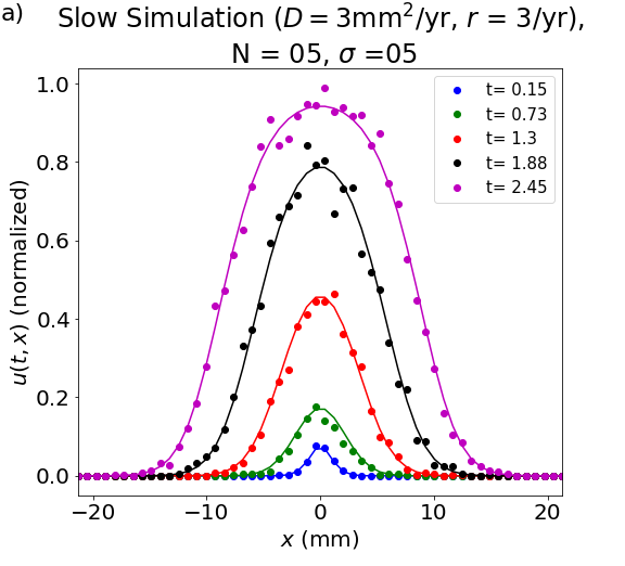
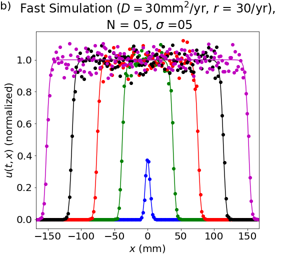
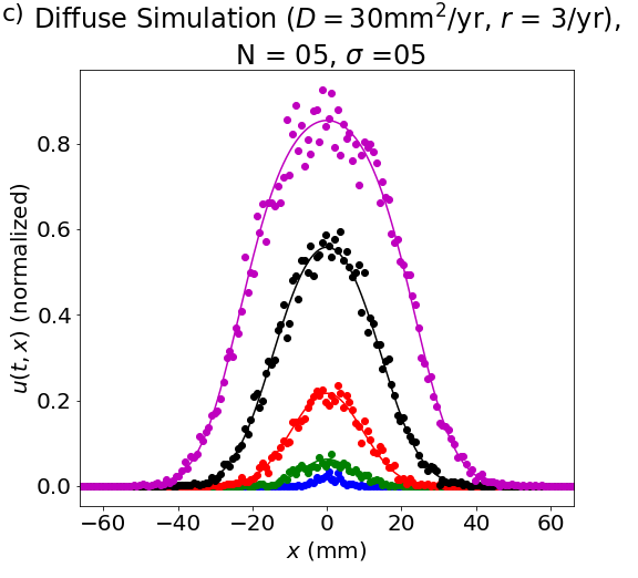
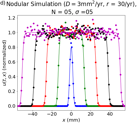
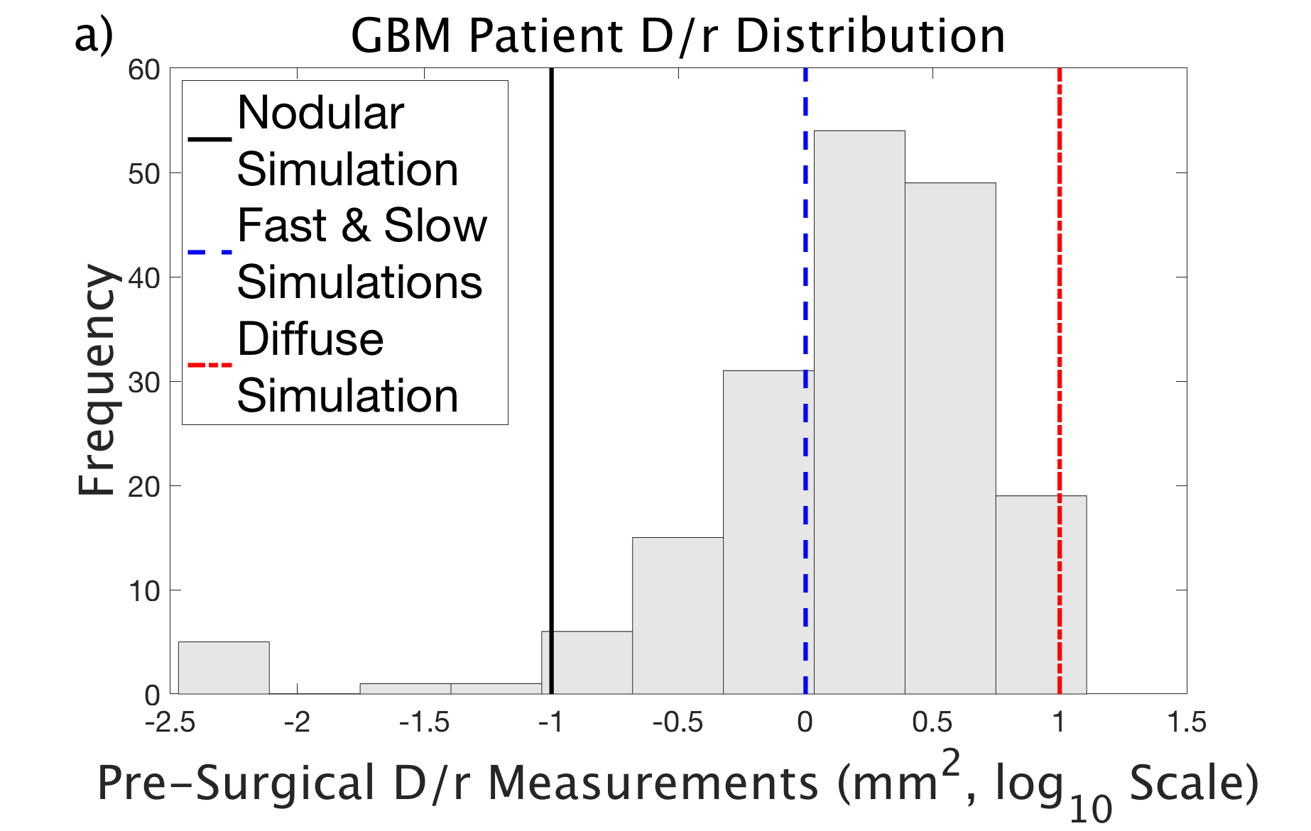
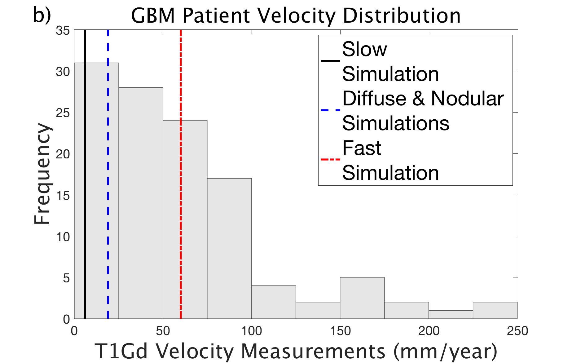
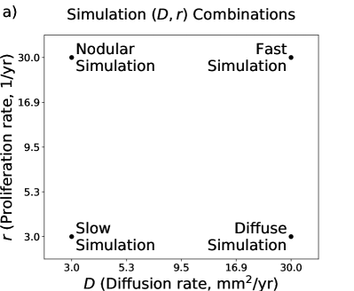
We are concerned with several data aspects in this study to investigate the performance of our methodology in the presence of biological data challenges. Namely, we vary the number of time samples , the parameter values parameterizing , whether data is sampled over the long or short time interval, as well as the noise level in the data. We will vary each of these values over the following domains: , , and . The units for ,, and are , , and year, respectively. We will refer to each of these combinations as slow, fast, diffuse, and nodular simulations, respectively. Figure 2 depicts resulting datasets from these four simulations over the long time interval. These simulation names and parameters are borrowed from a previous GBM modeling study hawkins-daarud_quantifying_2019 to cover the ranges of and that have been inferred for GBM patients. Figure 3 presents histograms of measured metrics of invasiveness () and velocities from 200 GBM patients as well as where the four simulations from this study fall in these distributions baldock_patient-specific_2014 ; neal2013_cancerresearch ; neal2013_plosone . Table 1 summarizes the range of parameters used in this study, as well as their labels used throughout.
| Variable | Realized Values | Labels |
|---|---|---|
| N | 3,5,10 | 3,5,10 |
| slow, fast, diffuse, nodular | ||
| 0.5,3 | short, long | |
| 0.01,0.05 | 1%,5% |
2.2 Data denoising
The first step in the equation learning process is data denoising and differentiation. Data denoising for equation learning refers to the process of approximating the solution and derivatives of an underlying dynamical system from a set of observed data. Previous methods relied on the use of finite differences for numerical differentiation in the case of noiseless data and polynomial splines in the presence of noise boninsegna2018sparse ; rudy_data-driven_2017 ; zhang2018robust . Lagergren et al. recently introduced a method that leverages artificial neural networks (ANNs) to be used for robust data smoothing and numerical differentiation in the presence of large amounts of noise and heteroscedastic data lagergren_learning_2020 .
A data denoising ANN, denoted by , is a differentiable function with inputs consisting of spatiotemporal points, , and outputs consisting of approximations for . The ANN is parameterized by the set consisting of weight matrices and bias vectors for where indicates the number of hidden layers or “depth” of the ANN. The size of each weight matrix and bias vector is determined by the number of neurons or “width” of the corresponding layer and its preceding layer. In particular, for the weight matrix and bias vector in the layer, the width of the layer determines the number of rows of the weight matrix while the width of the layer gives the number of columns and length of the weight matrix and bias vector, respectively. “Activation functions” (e.g. the sigmoid function ) are applied element-wise in between layers to introduce nonlinearity to the ANN.
With appropriately chosen activation functions, ANNs are in the class of functions known as universal function approximators hornik_1991 . In practice, this means that given large enough width and depth, ANNs can approximate any continuous function on a compact domain arbitrarily well. Therefore, following lagergren_learning_2020 , we use ANNs as surrogate models for the quantity of interest, . Back propagation of a trained ANN can be used for numerical differentiation, which is used to construct candidate terms for the equation learning task. See Figure 4 for a diagram of the data denoising procedure.
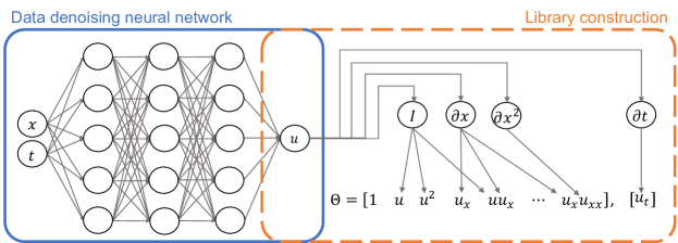
The ANN in this work is chosen to have three hidden layers with 256 neurons in each layer. This choice is large enough to give the ANN sufficient capacity to approximate the solution . Concretely, this ANN can be written as
| (8) |
where the weight matrices are denoted by , , and , bias vectors are denoted by , and , and activation functions are denoted by and . Note that (also called the “softplus” function) is specifically chosen to constrain neural network outputs to since we assume values of are non-negative.
The ANN parameters are optimized using the first-order gradient-based Adam optimizer kingma_adam_2017 with default parameters and batch-optimization. The ANN is trained by minimizing the objective function given by:
| (9) |
over the set of ANN parameters . The first term of Equation (9) corresponds to the generalized least squares error between the ANN and the observed noisy data . The second term acts as a regularization penalty to ensure ANN values stay between the minimum and maximum observed values of . We assume that is normalized so that . Note that in the small-time-sample limit (e.g. three time samples), the ANN can output unrealistic values between time samples. Therefore, for a given batch of data, the first term of Equation (9) is evaluated on the corresponding batch of observed data values while the second term is evaluated on a fixed grid spanning the input domain.
To prevent the ANN from overfitting to the data, the following measures are taken. The training data are randomly partitioned into 80%/20% training and validation sets. The network parameters are iteratively updated to minimize the error in Equation (9) on the training set. The network that results in the best error on the validation set is saved. Note that data from the validation set are never used to update network parameters. We use a small batch size of 10 to train each ANN. A small batch size acts as an additional form of regularization that (i) helps the ANN escape local minima during training and (ii) allows for better generalization keskar_large-batch_2017 . We employ early stopping of 1,000 (i.e. training ends if the validation error does not decrease for 1,000 consecutive epochs) to ensure convergence of each ANN independently.
The trained ANN is then used in the following Equation Learning step to build a library of candidate equation terms consisting of denoised values of and the approximated partial derivatives of . All network training and evaluation is implemented in Python 3.6.8 using the PyTorch deep learning library.
2.3 Equation learning, model selection, and equation post-processing
The second step of our equation learning methodology is to infer several candidate models to describe the data’s dynamics. From the approximations of and its partial derivatives from the ANN, we use the PDE-FIND algorithm rudy_data-driven_2017 to infer data-driven governing equations. This algorithm consists of first building a large library of candidate terms for the inferred model and then selecting which of these terms to include in the final model.
The PDE-FIND algorithm builds a library of potential right hand side terms in the matrix, . The columns of are comprised of candidate terms for the final inferred models. We use a library consisting of ten terms given by
From the PDE-FIND algorithm then recovers which terms should be included in the final inferred model by solving the linear system
| (10) |
where is a sparse vector parameterizing the final inferred differential equation model. Nonzero elements of correspond to relevant right hand side terms of the inferred model. Sparse linear regression methods are used to solve Equation (10) sparsely to ensure that the final recovered model is simple and contains a small number of terms. Following our previous study lagergren_learning_2020 , we use the adaptive forward-backward Greedy algorithm to estimate zhang2009adaptive . This algorithm requires estimation of the optimal tolerance with which to solve Equation (10); to estimate this hyperparameter, we randomly split the spatiotemporal domain into 50%/50% training and validation sets. Our previous study showed that small but systematic biases from the ANN can lead to incorrect terms being inferred, so we incorporate a round of “pruning” after solving Equation (10). During this round of pruning, we check the sensitivity of the mean-squared error to each nonzero entry in . The term of is included in the final inferred equation if increases by 5%, where is a copy of that is missing the term and is the estimated parameter vector in the absence of this term. The PDE-FIND algorithm is sensitive to the training-validation split of the spatiotemporal domain, so we infer 100 equations from 100 random training-validation domains and choose the three most common forms as the final inferred equations.
The third step of our equation learning methodology is model selection and post-processing of these inferred equations. To select which of the three top models best describes a given dataset, we implement the following model selection procedure. We perform forward simulations of these three top models starting with initial conditions from the first time sample, . Numerical implementation of the inferred equations is discussed in Appendix A. From these three models, we select the model with the lowest AIC score when compared to data at the final time sample as our selected model. The AIC here is advantageous because when two models lead to similar outputs, it will select the simpler model and avoid complex models. We include some post-processing of this model to ensure that the final model is interpretable. In particular, we ensure that the transport terms in the final recovered model can be written in a flux formulation and in turn conserve mass. For example, the diffusion term by itself can be re-written as and is thus in conservation form. The term by itself cannot be re-written in conservation form so it would be manually removed. If the two terms and are simultaneously recovered, then we keep both terms because .
2.4 Parameter Estimation and Uncertainty Quantification
We will consider the performance of the PDE-FIND algorithm in parameter estimation for a given data set by solving Equation (10) where is composed of the terms in Fisher-KPP Equation. We build the two column library of terms given by and solve the linear system using the linalg.lstsq function in the Python Numpy subpackage. We perform this computation for 100 separate training sets comprised of 50% of the spatiotemporal domain to determine how much these parameter estimates vary. This method of randomly selecting several subsambles of the domain for uncertainty quantification is known as subagging (a sobriquet for subsample aggregrating) buhlmann_bagging_2012 . We set our parameter estimate to be the median of these 100 estimates, and we set its normalized standard error to be the standard error of these estimates divided by the median value.
3 Results
We investigate the performance of our equation learning methodology in the presence of sparse time sampling over both the short and long timescales. We exhibit these results using artificial data sets simulated from the four simulations described in Table 1. Equation inference is discussed in Section 3.1, and parameter estimation and uncertainty quantification when the underlying equation is known are discussed in Section 3.2.
3.1 Equation Discovery
We test the performance of our equation learning method on artificial data that has been generated from all four simulations for N = 3, 5, or 10 time samples over both the short (0-0.5 years) and long (0-3 years) timescales with 1% noise (Table 2) and 5% noise levels (Table 5 in Appendix B). We investigate whether our equation learning methodology is able to infer the Fisher-KPP data from noisy data and how well the final inferred equations describe the true underlying dynamics. We test the model’s predicted dynamics by investigating both how the inferred models match the dynamics they were trained on and how the models predict system dynamics that they were not trained on. We further consider our methodology’s ability to infer the correct underlying equation form over a finer range of values in Section 3.1.3.
| Slow Simulation | |||
|---|---|---|---|
| Learned Equation (0-0.5 years) | Learned Equation (0-3 years) | ||
| 01 | 03 | ||
| 01 | 05 | ||
| 01 | 10 | ||
| Diffuse Simulation | |||
| Learned Equation (0-0.5 years) | Learned Equation (0-3 years) | ||
| 01 | 03 | ||
| 01 | 05 | ||
| 01 | 10 | ||
| Fast Simulation | |||
| Learned Equation (0-0.5 years) | Learned Equation (0-3 years) | ||
| 01 | 03 | ||
| 01 | 05 | ||
| 01 | 10 | ||
| Nodular Simulation | |||
| Learned Equation (0-0.5 years) | Learned Equation (0-3 years) | ||
| 01 | 03 | ||
| 01 | 05 | ||
| 01 | 10 | ||
3.1.1 Learning equations from data with 1% noise
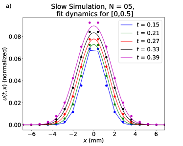
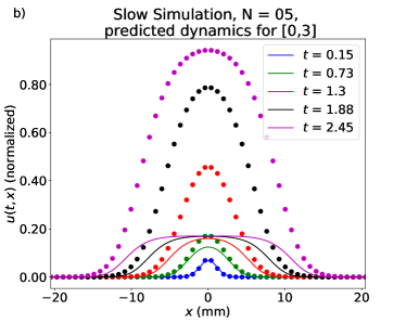
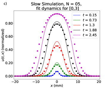
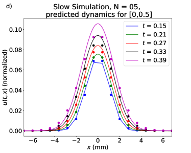
All final inferred equations for 1% noisy data are presented in Table 2. Table cells are highlighted in green when the correct underlying equation form (i.e., the Fisher-KPP Equation) is inferred. We also tested the ability of the inferred equations with time samples to match the dynamics they were trained on and predict dynamics on a separate time interval (Figures 5 and 8-10 in Appendix C).
The slow simulation on the short time scale.
For noisy data sampled over the short time interval for the slow simulation, our equation learning methodology infers the Fisher-KPP Equation with and time samples. With points, the Fisher-KPP Equation is not inferred. In Figure 5a, we simulated the inferred equation for time samples over the short time scale and observe that this equation accurately matches the true underlying dynamics. When this same equation is simulated over the long time scale, it does not accurately describe the true underlying dynamics (Figure 5b).
The slow simulation on the long time scale.
For noisy data sampled over the long time interval for the slow simulation, our equation learning methodology infers the Fisher-KPP Equation for all values of considered. In Figure 5c we simulate the inferred equation for time samples over the long time scale. The simulation matches the true dynamics well in many areas, although there is some disparity at and years for . When this same equation is simulated over the short time scale it accurately matches the true underlying dynamics (Figure 5d).
The diffuse simulation on the short time scale.
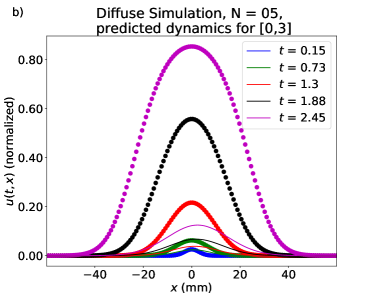
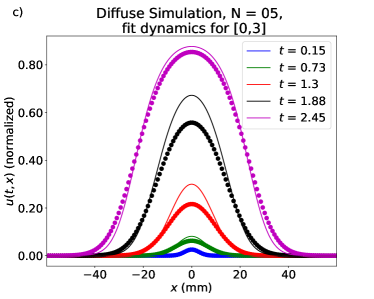
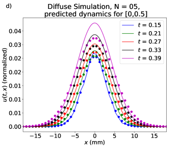
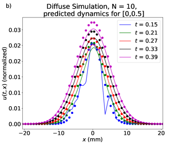
For noisy data sampled over the short time interval for the diffuse simulation, our equation learning methodology does not infer the correct underlying equation for any of the chosen values of . In Figure 8 in Appendix C, we simulated the inferred equation for time samples over the short time scale and observe that this equation does not match the true underlying dynamics. When this same equation is simulated over the long time scale, it does not accurately describe the true underlying dynamics.
The diffuse simulation on the long time scale.
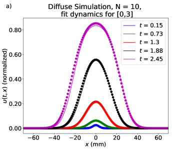
For noisy data sampled over the long time interval for the diffuse simulation, our equation learning methodology infers the Fisher-KPP Equation for all values of considered. In Figure 8, we simulate the inferred equation for time samples over the long time scale. The simulation matches the true dynamics qualitatively well in many areas. When this same equation is simulated over the short time scale, it accurately matches the true underlying dynamics.
The fast simulation on the short time scale.
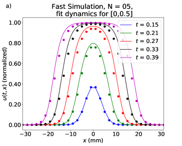
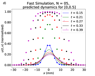
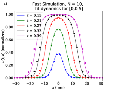
For noisy data sampled over the short time interval for the fast simulation, our equation learning methodology infers the Fisher-KPP Equation for and and does not infer the Fisher-KPP Equation for . In Figure 9 in Appendix C, we simulated the inferred equation for time samples over the short time scale and observe that the inferred equation accurately describes the true underlying dynamics. When this same equation is simulated over the long time scale, it accurately matches the true underlying dynamics.
The fast simulation on the long time scale.
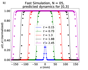
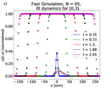
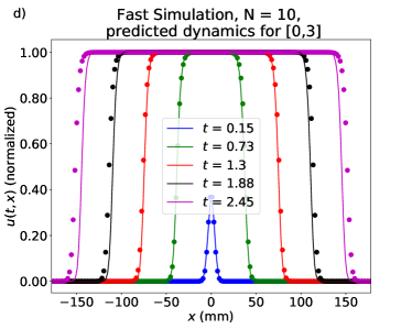
For noisy data sampled over the long time interval for the fast simulation, our equation learning methodology does not infer the correct underlying equation for any of the chosen values of . In Figure 9 in Appendix C, we simulated the inferred equation for time samples over the long time scale and observe that this equation does not accurately describe the true underlying dynamics. When this same equation is simulated over the short time scale, it does not accurately describe the true underlying dynamics.
The nodular simulation on the short time scale.
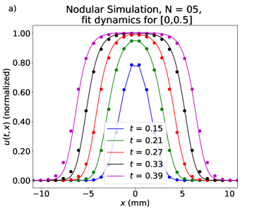
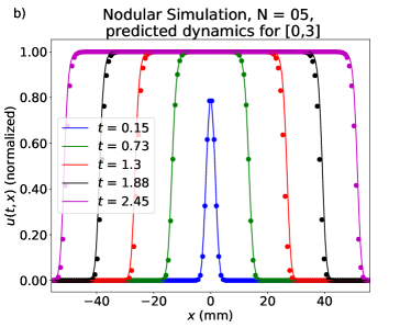
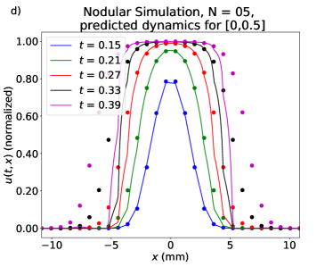
For noisy data sampled over the short time interval for the nodular simulation, our equation learning methodology infers the Fisher-KPP Equation for all values of considered. In Figure 10 in Appendix C, we simulated the inferred equation for time samples over the short time scale and observe that the inferred equation accurately describes the true underlying dynamics. When this same equation is simulated over the long time scale, it accurately matches the true underlying dynamics.
The nodular simulation on the long time scale.
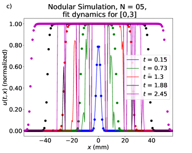
For noisy data sampled over the long time interval for the nodular simulation, our equation learning methodology does not infer the correct underlying equation for any of the chosen values of . In Figure 10 in Appendix C, we simulated the inferred equation for time samples over the long time scale and observe that this equation does not accurately describe the true underlying dynamics. When this same equation is simulated over the short time scale, it does not accurately describe the true underlying dynamics.
3.1.2 Learning equations from data with 5% noise
All final inferred equations for 5% noisy data are presented in Table 5 in Appendix B. Table cells are highlighted in green when the correct underlying equation form (i.e., the Fisher-KPP Equation) is inferred. We will also test the ability of the inferred equations with time samples to match the dynamics they were trained on and predict dynamics on a separate time interval (Figure 11 in Appendix C).
The slow simulation on the short time interval.
For noisy data sampled over the short time interval for the slow simulation, our equation learning methodology does not infer the correct underlying equation for any values of considered. Simulating the inferred equation for time samples over the short time scale does not lead to an accurate description of the true underlying dynamics on the short time interval or prediction of the true dynamics on the long time interval.
The slow simulation on the long time interval.
Over the long time interval, our equation learning methodology does infer the Fisher-KPP Equation with time samples. Simulating the inferred equation for time samples over the long time scale accurately matches the true underlying dynamics on the long time interval and accurately predicts the true dynamics on the short time interval.
The diffuse simulation on the short time interval.
For noisy data sampled over the short time interval for the diffuse simulation, our equation learning methodology does not infer the correct underlying equation for any values of considered. Simulating the inferred equation for time samples over the short time scale does not lead to an accurate description of the true underlying dynamics on the short time interval or prediction of the true dynamics on the long time interval.
The diffuse simulation on the long time interval.
Over the long time interval, our equation learning methodology does infer the Fisher-KPP Equation with time samples. Simulating the inferred equation for time samples over the long time scale accurately matches the true underlying dynamics on the long time interval and accurately predicts the true dynamics on the short time interval (Figure 11 in Appendix C).
The fast simulation on the short time interval.
For noisy data sampled over the short time interval for the fast simulation, our equation learning methodology infers the Fisher-KPP Equation with time samples. Simulating the inferred equation for time samples over the short time scale accurately matches the true underlying dynamics on the short time interval and accurately predicts the true dynamics on the long time interval (Figure 11 in Appendix C).
The fast simulation on the long time interval.
Over the long time interval, our equation learning methodology does not infer the correct underlying equation for any values of considered. Simulating the inferred equation for time samples over the short long scale does lead to an accurate description of the true underlying dynamics on the long time interval or prediction of the true dynamics on the short time interval.
The nodular simulation on the short time interval.
For noisy data sampled over the short time interval for the nodular simulation, our equation learning methodology infers the Fisher-KPP Equation with time samples. Simulating the inferred equation for time samples over the short time scale does not lead to an accurate description of the true underlying dynamics on the short time interval or prediction of the true dynamics on the long time interval.
The nodular simulation on the long time interval.
Over the long time interval, our equation learning methodology infers the Fisher-KPP Equation with time samples. Simulating the inferred equation for time samples over the long time scale accurately matches the true underlying dynamics on the long time interval and accurately predicts the true dynamics on the short time interval.
3.1.3 Learning equations for intermediate values
Recall that the four considered simulations in this study correspond to values representing somewhat extreme examples of estimated values from a cohort of GBM patients wang_prognostic_2009 . In this section, we investigate the performance of our equation learning methodology for intermediate values of and from 1% noisy data with time samples. Here we are interested in if we can infer the correct equation form, and score the accuracy of an inferred model form using the True Positive Ratio (TPR) given by:
| (11) |
where “TP” stands for true positives (nonzero terms in the final inferred equation that are nonzero), “FP” stands for false positives (nonzero terms in the final inferred equation that are zero), and “FN” stands for false negatives (zero terms in the final inferred equation that are nonzero). Note that a score of TPR = 1 indicates that the correct underlying equation form has been recovered and a TPR score less than 1 indicates that the incorrect underlying equation form has been recovered.
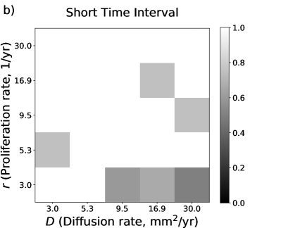
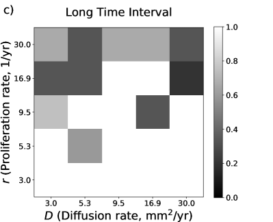
We inferred the equations underlying such data over 25 different combinations (Figure 6). We let both and vary over five values from a log-scale between their lower and upper values from Table 1. Over the short time interval, the correct underlying form is often inferred for larger values of ( /year), but is not usually inferred for /year. Over the long time interval, the correct underlying form is often inferred for smaller values of ( /year), but is not usually inferred for or 30.0 /year.
3.2 Parameter Estimation and Uncertainty Quantification
We investigated parameter estimation accuracy and uncertainty quantification using the PDE-FIND algorithm when we know that the underlying form is the Fisher-KPP Equation. Results using data from the short time interval are presented in Section 3.2.1 and the long time interval in Section 3.2.2.
3.2.1 Parameter Estimation and Uncertainty Quantification over the short time interval
We investigated the performance of the PDE-FIND algorithm for parameter estimation and uncertainty quantification with 5% noise and time samples on the short time interval (Table 3) for the parameters and . The fast simulation has the most accurate parameter estimation results on this time interval with error rates for and of 4.7% and 0.5%, respectively. The nodular simulation has error rates for and of 19.8% and 4.7%, respectively. The error rates for from the slow and diffuse simulations have error rates of 30.4% and 21.8%, respectively. PDE-FIND estimates with an error rate of 69.1% for the slow simulation and 25.1% for the diffuse simulation. The normalized standard errors, defined as the standard error of the parameter estimates divided by their median value, for fall between 0.012-0.062 for all four simulations, and the more inaccurate estimates tend to exhibit higher normalized standard errors here. The normalized standard errors for are higher, as they fall between 0.084-.25 for all four simulations, demonstrating that this method exhibits higher variation in estimating than in estimating . The fast simulation yields the smallest normalized standard error of 0.084 while the slow simulation yields the highest normalized standard error of 0.25.
| Parameter | True | Median | % Error | Normalized SE | |
|---|---|---|---|---|---|
| Slow Simulation | 3 | 0.928 | 69.1% | 0.25 | |
| 3 | 2.089 | 30.4% | 0.059 | ||
| Fast Simulation | 30 | 31.422 | 4.7% | 0.084 | |
| 30 | 29.84 | 0.5% | 0.012 | ||
| Diffuse Simulation | 30 | 22.462 | 25.1% | 0.132 | |
| 3 | 2.345 | 21.8% | 0.062 | ||
| Nodular Simulation | 3 | 3.595 | 19.8% | 0.227 | |
| 30 | 28.588 | 4.7% | 0.027 |
3.2.2 Parameter Estimation and Uncertainty Quantification over the long time interval
We investigated the performance of the PDE-FIND algorithm for parameter estimation and uncertainty quantification with 5% noise and time samples on the long time interval (Table 4) for the parameters and . The smallest parameter estimate error rates are found for the diffuse simulation with error rates of 4.4 and 11.8% for and , respectively. PDE-FIND estimates with small error rates between 6.0-9.4% error for the remaining simulations. The error rates for the remaining simulations for fall between 25.4-32.7%. The diffuse simulation yields the lowest normalized standard error for of 0.012, while the fast simulation yields the highest normalized standard error of 0.047. The diffuse simulation yields the smallest normalized standard error for of 0.101 while the fast and nodular simulations yield the highest normalized standard errors for of 0.248.
| Parameter | True | Median | % Error | Normalized SE | |
|---|---|---|---|---|---|
| Slow Simulation | 3 | 2.063 | 31.2% | 0.168 | |
| 3 | 2.786 | 7.1% | 0.02 | ||
| Fast Simulation | 30 | 37.624 | 25.4% | 0.248 | |
| 30 | 28.189 | 6.0% | 0.047 | ||
| Diffuse Simulation | 30 | 28.681 | 4.4% | 0.101 | |
| 3 | 2.646 | 11.8% | 0.012 | ||
| Nodular Simulation | 3 | 2.02 | 32.7% | 0.248 | |
| 30 | 27.166 | 9.4% | 0.023 |
4 Discussion
We investigated the performance of our equation learning methodology in equation inference, dynamics prediction, and parameter estimation from noisy data over a range of common challenges presented by biological data. These challenges include a wide variation in parameter values, sparse data sampling, and large amounts of noise. We used artificial data that has been generated from the Fisher-KPP Equation throughout this study due to the broad applicability of this model for many biological phenomena, including tumor progression and species invasion. The diffusion and proliferation values considered in this work correspond to the ranges of measured values from GBM patients wang_prognostic_2009 .
We observe in Table 2 that this methodology successfully recovers the correct underlying equation for the slow and diffuse simulations when data is observed on a long time interval of 0-3 years. The correct underlying form can be recovered with as few as three time samples on this time interval. Over the shorter time interval of 0-0.5 years, however, this methodology often either infers an incorrect equation form or infers the correct equation form with poor parameter estimates for these two simulations. With ten time samples from the slow simulation, for example, this methodology infers an equation with a carrying capacity that is ten times smaller than the true carrying capacity. Similarly, the inferred equation for the diffuse simulation will grow unbounded. These two simulations share a low proliferation rate of 3/year, suggesting that these simulations only exhibit their linear dynamics on the short interval and thus require the longer time interval for equation learning methods to accurately infer their nonlinear dynamics. These conclusions are supported by observing that the inferred equations from data that is sampled over the longer time interval can still accurately predict the system dynamics on the shorter time interval.
Alternatively, our equation learning methodology successfully recovers the correct underlying equations for the fast and nodular simulations over the shorter time interval of 0-0.5 years. These two simulations share a high growth rate (30/year), suggesting that the systems’ nonlinear dynamics are sufficiently sampled over the shorter time interval for successful equation recovery from equation learning methods. The inferred equations on this shorter time interval generalize well to predict the true underlying dynamics on the long time interval of 0-3 years. Our equation learning methodology does not infer the correct underlying equation for these two simulations when data is sampled over the long time interval. We observe in Figure 2 that these simulations appear to have converged to their traveling wave profiles between the first and second time samples of the long time interval. Traveling waves are a known problem for the PDE-FIND algorithm because multiple reaction-diffusion-advection equations will lead to traveling wave solutions. A previous study proposed simulating bimodal data to distinguish between the advection equation and the Korteweg-de Vries Equation rudy_data-driven_2017 . Here, we propose that sampling the dynamics before a traveling wave profile has been attained can lead to accurate equation inference for the Fisher-KPP Equation.
For low noise () data, the final inferred equation form appears robust to the number of time samples. When data is observed over the correct time interval, then the final equation form typically does not change between three and ten time samples (Table 2). An exception is the fast simulation, which needed five or ten time samples to recover the correct underlying equation. With a larger amount of noise (), the final inferred equation appears more sensitive to the the number of observed time samples. For example, the slow simulation required five or ten time samples to infer the correct underlying equation and the fast simulation required ten time samples to infer the correct underlying equation. Interestingly, our equation learning methodology inferred the correct equation for the diffuse and nodular simulations with three time samples with 5% noise but inferred incorrect equation forms for these two simulations with five or ten time samples. We note, however, that the extra terms for the diffuse simulation here correspond to backwards negative nonlinear diffusion and advection which a user may manually neglect if found in practice. Furthermore, we could have had more success recovering the correct equation form by tuning hyperparameters (such as the pruning percentage) here, but we instead focus on a flexible technique that provides users with interpretable equations for users to then alter if needed.
The four simulations considered throughout this work correspond to the outer ranges of diffusion and proliferation observed in GBM patients. We further demonstrated in Figure 6 that our equation learning methodology is successful in recovering the correct equation learning methodology for many intermediate values. Typically, our methodology has more success in accurate equation inference for larger values of (/year) on the short time interval and for smaller values of (/year) on the longer time interval for 1% noisy data.
Equation learning is promising technique for parameter estimation and uncertainty quantification due to having a low computational expense. For example, solving Equation (10) for does not require solving a differential equation, whereas typical parameter estimation routines require numerous differential equation model simulations banks2014modeling . We observe that parameter estimation appears more accurate for the slow and diffuse simulations over the long time interval than for the short time interval. Similarly, parameters are more accurate for the fast and nodular simulations over the short time interval than the long time interval. Such methods could be used to obtain computationally inexpensive initial parameter estimates for frequentist parameter estimation approaches approaches or for prior distribution specification for Bayesian inference routines hawkins-daarud_quantifying_2019 . Parameter uncertainty has been proposed previously as a measure to infer the top equation form from several plausible candidates zhang2018robust . In support of this proposal, we observe in our work that smaller amounts of parameter uncertainty result when data is sampled over an appropriate time interval.
5 Conclusion
Methods from equation learning have the potential to become invaluable tools for researchers in developing data-driven models, and in turn understanding the mechanics underlying a biological process, estimating parameters, and predicting previously-unknown system dynamics. Before such methods become commonplace in the mathematical biology field, however, it is crucial to thoroughly investigate the performance of such methods in the presence of common challenges that biological data presents. We have scrutinized the performance of a state-of-the-art equation learning methodology in the presence of such challenges in this work. This equation learning methodology is composed of a data denoising step with an ANN, equation learning through the PDE-FIND algorithm lagergren_learning_2020 ; rudy_data-driven_2017 , and a final step comprised of model selection and post-processing to ensure the inferred equation is simple and biologically interpretable.
The biological data challenges considered in this work include sparse sampling of data, a small number of time samples, parameter heterogeneity, and large noise levels. Our equation learning method can recover the correct equation from data with a small number of time samples when the data is sampled over an appropriate time interval. Our methodology can also reliably predict previously-unobserved dynamics when trained over an appropriate time interval. When this methodology is not trained over an appropriate time interval, however, the inferred equation and predicted dynamics are not reliable. Determining when to sample the data for accurate inference in this work crucially depends on the intrinsic growth rate of populations: fast-growing populations require data sampling on a short time interval and slow-growing populations require sampling on a long time interval for accurate inference. When sampled over the correct time interval, datasets exhibited a combination of both initial linear model dynamics and long-term nonlinear model dynamics. Such results suggest that an informative time interval for equation learning methods should include both of these phases for accurate inference. Noisier data requires more time samples for accurate recovery: we observed in this work that three time samples were often sufficient for accurate inference of 1% noisy data, but ten time samples were required for such inference on 5% noisy data. Deciphering when equation learning methodologies are reliable in the presence of practical data challenges is important for biological research to ensure these methods are not used to make incorrect inference for a system under study. The challenges addressed in this study are prevalent in biological research, where expensive or challenging data collection may limit us to sparse datasets baldock_patient-specific_2014 or measurement is often corrupted by noise perretti_model-free_2013 .
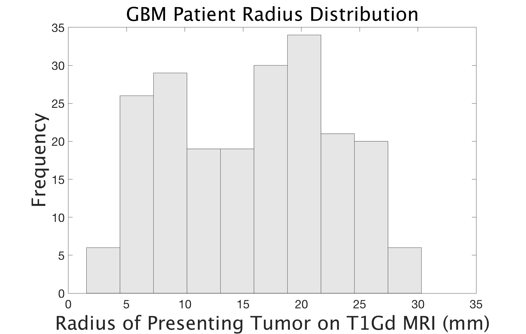
The values of diffusion and intrinsic growth considered in this work correspond to the ranges of these values that have been measured from GBM patients’ MR images wang_prognostic_2009 . In Figures 3 and 7, we depict histograms of measured ratios, T1Gd velocities, and tumor radii from GBM patients before surgery. If one is interested in inferring the dynamics from patient data to inform treatment decisions for improved prognosis or predicted dynamics, then patient-estimated tumor velocity measurements can be combined with the results from this study to determine how reliable the inferred equation may be. A patient’s tumor could be matched to one of the four simulations considered in this work based on their measured and velocity estimates (for example, if the tumor has a high value and low velocity, then this tumor may correspond to the slow simulation). If patient data has been observed on an appropriate time interval for inference (a longer time interval for slow and diffuse simulations, a shorter time interval for fast and nodular simulations), then one may have a high degree of confidence in the inferred equation and dynamics. If patient data has not been observed on an appropriate time interval for inference, then the inferred equation and dynamics might not be sufficiently supported by the data. We also observed in this work that if the population dynamics are primarily observed after the population has reached confluence, then the inferred dynamics may not be reliable. The tumor radius histogram in Figure 7 can be used to further determine whether or not observed patient data has already reached its carrying capacity and is suitable for inference from equation learning methods.
We focused on inference of the Fisher-KPP Equation in this work due to its wide use in the biological literature hastings_spatial_2005 ; hawkins-daarud_quantifying_2019 ; nardini_investigation_2018 . Previous equation learning studies have also successfully inferred other common models in biology, including transport equations lagergren_learning_2020 , pattern-forming reaction-diffusion equations rudy_data-driven_2017 , and compartmental epidemiological models mangan2017model . We expect that the results, methodology, and open-source code presented in this work will enable other researchers to assess whether equation learning methods can be applied to a wide array biological data.
This work proposes many areas for future research for mathematicians and data scientists working on computational methods and modeling for biological data. We observed that changing the parameters of a mathematical model influences the spatiotemporal domain over which the PDE-FIND algorithm can successfully recover the correct underlying equation. Future research should aim to infer what an informative domain may be for general ODE and PDE systems as well as methods to determine if datasets contain high or low information content for equation learning. As an example, only sampling near an equilibrium solution will likely lead to a learned model of , whereas only sampling far away from stable equilibria may neglect nonlinear dynamics in the final learned model. It will be interesting to further investigate what combinations of transient and long-term dynamics are sufficient for accurate inference from biological systems data, which may be difficult or expensive to collect. Improvements in data denoising and equation learning methods will further inform this work. A recent neural network architecture, termed a “Physics-informed neural network”, simultaneously denoises data and estimates the parameters under the assumption that the model is known raissi_hidden_2018 . The simultaneous denoising of data and equation inference will likely improve both methods and is thus an important area for future research.
Appendix A Simulating a learned Equation
To simulate the inferred equation represented by the sparse vector , we begin by removing all zero terms from as well as the corresponding terms from . We can now define our inferred dynamical systems model as
| (12) |
We use the method of lines approach to simulate this equation, in which we discretize the right hand side in space and then integrate along the dimension. The Scipy integration subpackage (version 1.4.1) is used to integrate this equation over time using an explicit fourth order Runge-Kutte Method. We ensure that the simulation is stable by enforcing the CFL Condition for an advection equation with speed is satisfied, e.g., . Some inferred equations may not be well-posed, e.g., . If the time integration fails at any point, we manually set the model output to everywhere to ensure this model is not selected as a final inferred model.
For the final inferred columns of , we define nonlinear stencils, such that . As an example, we an upwind stencil leveque_finite_2007 for first order derivative terms, such as , so that . We use a central difference stencil for . For multiplicative terms, we define the stencil for as where denotes element-wise multiplication so that . Similarly, we set , etc.
Appendix B Learning the 1d Fisher-KPP Equation with 5% noisy data
In Table 5, we present the inferred equations for all 1d data sets considered with .
| Slow Simulation | |||
| Learned Equation (0-0.5 years) | Learned Equation (0-3 years) | ||
| 05 | 03 | ||
| 05 | 05 | ||
| 05 | 10 | ||
| Diffuse Simulation | |||
| Learned Equation (0-0.5 years) | Learned Equation (0-3 years) | ||
| 05 | 03 | ||
| 05 | 05 | ||
| 05 | 10 | ||
| Fast Simulation | |||
| Learned Equation (0-0.5 years) | Learned Equation (0-3 years) | ||
| 05 | 03 | ||
| 05 | 05 | ||
| 05 | 10 | ||
| Nodular Simulation | |||
| Learned Equation (0-0.5 years) | Learned Equation (0-3 years) | ||
| 05 | 03 | ||
| 05 | 05 | ||
| 05 | 10 | ||
Appendix C Fit and Predicted Dynamics
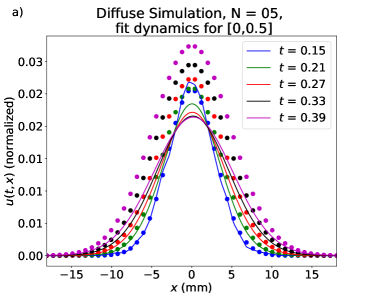
The fit and predicted system dynamics for the diffuse, fast, and nodular s with 1% noise and time samples are depicted in Figures 8-10, respectively. The fit and predicted dynamics for the Diffuse and fast s with 5% noise and time samples are depicted in Figures 11.
References
- (1) Akaike, H.: A new look at the statistical model identification. IEEE Transactions on Automatic Control 19(6), 716–723 (1974). DOI 10.1109/TAC.1974.1100705. Conference Name: IEEE Transactions on Automatic Control
- (2) Akaike, H.: Information theory and an extension of the maximum likelihood principle. In: E. Parzen, K. Tanabe, G. Kitagawa (eds.) Selected papers of Hirotugu Akaike, Springer Series in Statistics, pp. 199–213. Springer New York, New York, NY (1998). DOI 10.1007/978-1-4612-1694-0˙15
- (3) Baldock, A.L., Ahn, S., Rockne, R., Johnston, S., Neal, M., Corwin, D., Clark-Swanson, K., Sterin, G., Trister, A.D., Malone, H., Ebiana, V., Sonabend, A.M., Mrugala, M., Rockhill, J.K., Silbergeld, D.L., Lai, A., Cloughesy, T., Ii, G.M.M., Bruce, J.N., Rostomily, R.C., Canoll, P., Swanson, K.R.: Patient-specific metrics of invasiveness reveal significant prognostic benefit of resection in a predictable subset of gliomas. PLoS ONE 9(10), e99057 (2014). DOI 10.1371/journal.pone.0099057
- (4) Banks, H.T., Catenacci, J., Hu, S.: Use of difference-based methods to explore statistical and mathematical model discrepancy in inverse problems. J Inverse Ill Posed Probl 24(4), 413–433 (2016)
- (5) Banks, H.T., Hu, S., Thompson, W.C.: Modeling and inverse problems in the presence of uncertainty. Chapman and Hall/CRC (2014)
- (6) Boninsegna, L., Nüske, F., Clementi, C.: Sparse learning of stochastic dynamical equations. J Chem Phys 148(24), 241723 (2018)
- (7) Bortz, D.M., Nelson, P.W.: Model selection and mixed-effects modeling of HIV infection dynamics. Bull. Math. Biol. 68(8), 2005–2025 (2006). DOI 10.1007/s11538-006-9084-x
- (8) Brunton, S.L., Proctor, J.L., Kutz, J.N.: Discovering governing equations from data by sparse identification of nonlinear dynamical systems. PNAS 113(15), 3932–3937 (2016). DOI 10.1073/pnas.1517384113
- (9) Buhlmann, P.: Bagging, boosting and ensemble methods. In: J.E. Gentle, W.K. Härdle, Y. Mori (eds.) Handbook of computational statistics: concepts and methods, Springer handbooks of computational statistics, pp. 985–1022. Springer, Berlin, Heidelberg (2012). DOI 10.1007/978-3-642-21551-3˙33
- (10) Burnham, K.P., Anderson, D.R., Burnham, K.P.: Model selection and multimodel inference: a practical information-theoretic approach, 2nd ed edn. Springer, New York (2002)
- (11) Dwyer, G., Elkinton, J.S., Hajek, A.E.: Spatial scale and the spread of a fungal pathogen of gypsy moth. Am Nat 152(3), 485–494 (1998). DOI 10.1086/286185
- (12) Ferguson, N.M., Laydon, D., Nedjati-Gilani et al., G.: Impact of non-pharmaceutical interventions NPIs to reduce COVID-19 mortality and healthcare demand. pre-print (2020). DOI 10.25561/77482
- (13) Fisher, R.A.: The wave of advance of advantageous genes. Ann of Eugen 7, 353–369 (1937)
- (14) Francis, C.R.I.C., Hurst, R.J., Renwick, J.A.: Quantifying annual variation in catchability for commercial and research fishing. Fish Bull 101(2), 293–304 (2003)
- (15) Garcia-Ramos, G., Rodriguez, D.: Evolutionary speed of species invasions. Evolution 56(4), 661–668 (2002). DOI 10.1554/0014-3820(2002)056[0661:ESOSI]2.0.CO;2
- (16) Hastings, A., Cuddington, K., Davies, K.F., Dugaw, C.J., Elmendorf, S., Freestone, A., Harrison, S., Holland, M., Lambrinos, J., Malvadkar, U., Melbourne, B.A., Moore, K., Taylor, C., Thomson, D.: The spatial spread of invasions: new developments in theory and evidence. Ecol Lett 8(1), 91–101 (2005). DOI 10.1111/j.1461-0248.2004.00687.x
- (17) Hawkins-Daarud, A., Johnston, S.K., Swanson, K.R.: Quantifying uncertainty and robustness in a biomathematical model–based patient-specific response metric for glioblastoma. JCO Clin Cancer Inform 3, 1–8 (2019). DOI 10.1200/CCI.18.00066
- (18) Hornik, K.: Approximation capabilities of multilayer feedforward networks. Neural Netw 4(2), 251 – 257 (1991). DOI 10.1016/0893-6080(91)90009-T
- (19) Jin, W., Shah, E.T., Penington, C.J., McCue, S.W., Chopin, L.K., Simpson, M.J.: Reproducibility of scratch assays is affected by the initial degree of confluence: Experiments, modelling and model selection. J Theor Biol 390, 136–145 (2016). DOI 10.1016/j.jtbi.2015.10.040
- (20) Kaiser, E., Kutz, J.N., Brunton, S.L.: Sparse identification of nonlinear dynamics for model predictive control in the low-data limit. Proc R Soc A 474(2219), 20180335 (2018)
- (21) Keskar, N.S., Mudigere, D., Nocedal, J., Smelyanskiy, M., Tang, P.T.P.: On large-batch training for deep learning: Generalization gap and sharp minima. arXiv:1609.04836 [cs, math] (2017). URL http://arxiv.org/abs/1609.04836. ArXiv: 1609.04836
- (22) Kingma, D.P., Ba, J.: Adam: A method for stochastic optimization. arXiv:1412.6980 [cs] (2017). URL http://arxiv.org/abs/1412.6980. ArXiv: 1412.6980
- (23) Kolmogoroff, A., Petrovsky, I., Piscounoff, N.: Etude de l’equation de la diffusion avec croissance de la quantite de matiere et son application a un probleme biologique. Moscow Univ. Bull. Math 1, 1–25 (1937)
- (24) Lagergren, J.H., Nardini, J.T., Michael Lavigne, G., Rutter, E.M., Flores, K.B.: Learning partial differential equations for biological transport models from noisy spatio-temporal data. Proc R Soc A 476(2234), 20190800 (2020). DOI 10.1098/rspa.2019.0800
- (25) LeVeque, R.J.: Finite difference methods for ordinary and partial differential equations: steady-state and time-dependent problems. Society for Industrial and Applied Mathematics, Philadelphia, PA (2007)
- (26) Lubina, J.A., Levin, S.A.: The spread of a reinvading species: Range expansion in the California sea otter. Am Nat 131(4), 526–543 (1988)
- (27) Mangan, N.M., Kutz, J.N., Brunton, S.L., Proctor, J.L.: Model selection for dynamical systems via sparse regression and information criteria. Proc R Soc A 473(2204), 20170009 (2017)
- (28) Massey, S.C., White, H., Whitmire, P., Doyle, T., Johnston, S.K., Singleton, K.W., Jackson, P.R., Hawkins-Daarud, A., Bendok, B.R., Porter, A.B., Vora, S., Sarkaria, J.N., Hu, L.S., Mrugala, M.M., Swanson, K.R.: Image-based metric of invasiveness predicts response to adjuvant temozolomide for primary glioblastoma. PLoS ONE 15(3), e0230492 (2020). DOI 10.1371/journal.pone.0230492
- (29) Mori, Y., Jilkine, A., Edelstein-Keshet, L.: Wave-pinning and cell polarity from a bistable reaction-diffusion system. Biophys J 94(9), 3684–3697 (2008). DOI 10.1529/biophysj.107.120824
- (30) Murray, J.D.: Mathematical biology I. An introduction, 3rd edn. Springer New York, New York, NY (2002)
- (31) Nardini, J., Bortz, D.: Investigation of a structured Fisher’s equation with applications in biochemistry. SIAM J Appl Math 78(3), 1712–1736 (2018). DOI 10.1137/16M1108546
- (32) Nardini, J.T., Bortz, D.M.: The influence of numerical error on parameter estimation and uncertainty quantification for advective PDE models. Inverse Problems 35(6), 065003 (2019). DOI 10.1088/1361-6420/ab10bb
- (33) Nardini, J.T., Chapnick, D.A., Liu, X., Bortz, D.M.: Modeling keratinocyte wound healing: cell-cell adhesions promote sustained migration. J Theor Biol 400, 103–117 (2016). DOI 10.1016/j.jtbi.2016.04.015
- (34) Neal, M.L., Trister, A.D., Ahn, S., Baldock, A., Bridge, C.A., Guyman, L., Lange, J., Sodt, R., Cloke, T., Lai, A., Cloughesy, T.F., Mrugala, M.M., Rockhill, J.K., Rockne, R.C., Swanson, K.R.: Response classification based on a minimal model of glioblastoma growth is prognostic for clinical outcomes and distinguishes progression from pseudoprogression. Cancer Res 73(10), 2976–2986 (2013). DOI 10.1158/0008-5472.CAN-12-3588
- (35) Neal, M.L., Trister, A.D., Cloke, T., Sodt, R., Ahn, S., Baldock, A.L., Bridge, C.A., Lai, A., Cloughesy, T.F., Mrugala, M.M., Rockhill, J.K., Rockne, R.C., Swanson, K.R.: Discriminating survival outcomes in patients with glioblastoma using a simulation-based, patient-specific response metric. PLoS ONE 8(1), 1–7 (2013). DOI 10.1371/journal.pone.0051951
- (36) Ozik, J., Collier, N., Wozniak, J.M., Macal, C., Cockrell, C., Friedman, S.H., Ghaffarizadeh, A., Heiland, R., An, G., Macklin, P.: High-throughput cancer hypothesis testing with an integrated PhysiCell-EMEWS workflow. BMC Bioinform 19(18), 483 (2018). DOI 10.1186/s12859-018-2510-x
- (37) Perretti, C., Munch, S., Sugihara, G.: Model-free forecasting outperforms the correct mechanistic model for simulated and experimental data. PNAS 110, 5253–5257 (2013)
- (38) Raissi, M., Karniadakis, G.E.: Hidden physics models: Machine learning of nonlinear partial differential equations. J Comput Phys 357, 125–141 (2018). DOI 10.1016/j.jcp.2017.11.039
- (39) Rockne, R.C., Trister, A.D., Jacobs, J., Hawkins-Daarud, A.J., Neal, M.L., Hendrickson, K., Mrugala, M.M., Rockhill, J.K., Kinahan, P., Krohn, K.A., Swanson, K.R.: A patient-specific computational model of hypoxia-modulated radiation resistance in glioblastoma using 18f-FMISO-PET. J R Soc Interface 12(103), 20141174 (2015). DOI 10.1098/rsif.2014.1174
- (40) Rudy, S.H., Brunton, S.L., Proctor, J.L., Kutz, J.N.: Data-driven discovery of partial differential equations. Sci Adv 3(4), e1602614 (2017). DOI 10.1126/sciadv.1602614
- (41) Rutter, E.M., Stepien, T.L., Anderies, B.J., Plasencia, J.D., Woolf, E.C., Scheck, A.C., Turner, G.H., Liu, Q., Frakes, D., Kodibagkar, V., et al.: Mathematical analysis of glioma growth in a murine model. Sci Rep 7(2508) (2017)
- (42) Schwarz, G.: Estimating the dimension of a model. Ann Stat 6(2), 461–464 (1978). DOI 10.1214/aos/1176344136. Publisher: Institute of Mathematical Statistics
- (43) Ulmer, M., Ziegelmeier, L., Topaz, C.M.: A topological approach to selecting models of biological experiments. PLoS ONE 14(3), e0213679 (2019). DOI 10.1371/journal.pone.0213679
- (44) Urban, M.C., Phillips, B.L., Skelly, D.K., Shine, R., Wiens, A.E.J.J., DeAngelis, E.D.L.: A toad more traveled: The heterogeneous invasion dynamics of cane toads in Australia. Am Nat 171(3), E134–E148 (2008). DOI 10.1086/527494
- (45) Walter, E., Pronzato, L.: Qualitative and quantitative experiment design for phenomenological models—A survey. Automatica 26(2), 195–213 (1990). DOI 10.1016/0005-1098(90)90116-Y
- (46) Wang, C.H., Rockhill, J.K., Mrugala, M., Peacock, D.L., Lai, A., Jusenius, K., Wardlaw, J.M., Cloughesy, T., Spence, A.M., Rockne, R., Alvord, E.C., Swanson, K.R.: Prognostic significance of growth kinetics in newly diagnosed glioblastomas revealed by combining serial imaging with a novel biomathematical model. Cancer Res 69(23), 9133–9140 (2009). DOI 10.1158/0008-5472.CAN-08-3863
- (47) Warne, D.J., Baker, R.E., Simpson, M.J.: Using experimental data and information criteria to guide model selection for reaction–diffusion problems in mathematical biology. Bull Math Biol 81(6), 1760–1804 (2019). DOI 10.1007/s11538-019-00589-x
- (48) Zhang, S., Lin, G.: Robust data-driven discovery of governing physical laws with error bars. Proc R Soc A 474(2217), 20180305 (2018)
- (49) Zhang, S., Lin, G.: Robust subsampling-based sparse Bayesian inference to tackle four challenges (large noise, outliers, data integration, and extrapolation) in the discovery of physical laws from data. arXiv:1907.07788 [cs, stat] (2019). URL http://arxiv.org/abs/1907.07788. ArXiv: 1907.07788
- (50) Zhang, T.: Adaptive forward-backward greedy algorithm for sparse learning with linear models. In: Advances in Neural Information Processing Systems, pp. 1921–1928 (2009)