Bridging the Gap Between Training and Inference for Spatio-Temporal Forecasting

Abstract

Spatio-temporal sequence forecasting is one of the fundamental tasks in spatio-temporal data mining. It facilitates many real world applications such as precipitation nowcasting, citywide crowd flow prediction and air pollution forecasting. Recently, a few Seq2Seq based approaches have been proposed, but one of the drawbacks of Seq2Seq models is that, small errors can accumulate quickly along the generated sequence at the inference stage due to the different distributions of training and inference phase. That is because Seq2Seq models minimise single step errors only during training, however the entire sequence has to be generated during the inference phase which generates a discrepancy between training and inference. In this work, we propose a novel curriculum learning based strategy named Temporal Progressive Growing Sampling to effectively bridge the gap between training and inference for spatio-temporal sequence forecasting, by transforming the training process from a fully-supervised manner which utilises all available previous ground-truth values to a less-supervised manner which replaces some of the ground-truth context with generated predictions. To do that we sample the target sequence from midway outputs from intermediate models trained with bigger timescales through a carefully designed decaying strategy. Experimental results demonstrate that our proposed method better models long term dependencies and outperforms baseline approaches on two competitive datasets.

1 Introduction

Spatio-Temporal Sequence Forecasting (STSF) is one of the fundamental tasks in spatio-temporal data mining [19]. It facilitates many real world applications such as precipitation nowcasting [17], citywide crowd flow prediction [29, 4] and air pollution forecasting [27]. It is to predict future values based on a series of past observations. STSF is formally defined as below:

Definition 1.

Given a length-$T$ matrix sequence $\mathcal{S}=\left[\mathcal{X}_{1},\mathcal{X}_{2},\ldots,\mathcal{X}_{T}\right]$. Each matrix $\mathcal{X}_{t}\in\mathcal{S}$ consists of measurements of coordinates at time-step $t$. STSF is to predict a sequence of corresponding measurements of following $k$ time-steps based on the past observations of $\mathcal{S}$, denoted as $\hat{\mathcal{P}}=\left[\hat{\mathcal{X}}_{T+1},\hat{\mathcal{X}}_{T+2},\ldots,\hat{\mathcal{X}}_{T+k}\right]$.

With the recent advances of Seq2Seq model [21] in sequence modelling such as Neural Machine Translation (NMT) and speech recognition, researchers adapt Seq2Seq to model STSF as sequence modelling. In particular, both DCRNN [11] and PredRNN [25] utilised an RNN-based encoder to encode a source sequence $\mathcal{S}$ into a feature matrix, such feature matrix will then be decoded recursively conditioned on previous contexts into the target sequence $\hat{\mathcal{P}}$ with a separated RNN-based decoder. During the training phase, the previous contexts become ground-truth observations. However, during the inference phase, the previous contexts are drawn from the model itself as no ground-truth observations are available for the decoder. The cause of the discrepancy between the training and inference stages is so called exposure bias [14]. Resulting small errors caused by the bias are quickly accumulated to become a large error along the generated sequence at the inference stage. One intuitive solution is to unify the training and inference phases by using previously generated contexts instead of ground-truth values during training. However, this causes the model more difficult or even unable to converge [1, 22]. Bengio et al. introduced Scheduled Sampling [1] to overcome such problem by gradually transform between these two strategies which shows significant improvements and has been widely used in NMT systems. DCRNN and PredRNN adapt Scheduled Sampling into STSF which shows some improvements. However, we argue that simply adopting Scheduled Sampling from NMT to STSF is not ideal even though they both are for sequence modelling due to two clear distinctions. First, NMT system is basically for the word level classification problem that optimises the cross entropy loss conditioned on the source sequence and previous contexts, whereas STSF is for the regression problem that optimises a regression loss such as Mean Square Error (MSE) and Mean Absolute Error (MAE). Second, two consecutive words in NMT systems are semantically close to each other, and small errors caused by the training bias could result in a completely different translation. However, two measurements in two consecutive time steps in STSF are geographically close and contiguous to each other, errors make by previous steps could result a confusion to the local trend of prediction that leads to bigger gap to the long term predictions.

Motivated by the above observations, we bridge the gap between training and inference for spatio-temporal forecasting by introducing a novel coarse-to-fine hierarchical sampling method named Temporal Progressive Growing Sampling, in short TPG. The idea is to transform the training process from a fully-supervised manner which utilises all available previous ground-truth to a less-supervised manner which replaces some of the ground-truth contexts with generated predictions. To do that we also sample the target sequence from midway outputs from intermediate models trained with bigger timescales through a carefully designed decaying strategy. By doing so, the model explores the differences between the training and inference phases as well as the intermediate model in order to correct its exposure bias. Experimental results demonstrate our model achieves superior performance as well as faster convergence time on two spatio-temporal sequence forecasting datasets. Experiments also show that our proposed method is better at modelling long term dependencies hence our method produces better long term prediction accuracies.

Main contributions of this paper are summarised as follows:

• We propose a novel temporal progressive growing sampling method to effectively bridging the gap between training and inference for spatio-temporal forecasting. Model is trained with bigger time gap initially and gradually transform into smaller time gap.

• We carefully design a decay strategy that take account of current index of the sequence, the latter sequence with larger probability to be replaced by the generated predictions during training, which helps the convergence of the training and yield better performance.

• We conduct extensive experiments on two real-world spatio-temporal datasets to evaluate the performance of our proposed method. Experimental results reveal that our approach achieves superior performance on sequence forecasting tasks, and experimental results also show our approach achieve better long term prediction accuracies.

The rest of paper is organised as follows. Section 2 introduces our proposed TPG and discusses the details of our model. Section 3 and Section 4 present the experimental results of weather prediction, and with Moving MNIST dataset [20]. Then Section 5 draws links to some related studies. Lastly, Section 6 presents concluding remarks and lists several directions for future work.

2 Temporal Progressive Growing Sampling

2.1 Seq2Seq and Scheduled Sampling

Sequence to Sequence model (Seq2Seq) [21] was first introduced to solve complex sequential problems that traditional RNN approaches cannot model diverse input and output lengths. Seq2Seq is also known as an encoder-decoder where the encoder encodes the original sequence into a feature vector, then the decoder outputs a target sequence based on the feature vector and previous contexts. Typically, both encoder and decoder are RNN, and Seq2Seq has been used for sequence modeling tasks like NMT, speech recognition and recently for STSF tasks [11, 15, 28].

One of the main drawbacks of Seq2Seq models is that, small errors can accumulate quickly along the generated sequence at the inference stage due to the different distributions of training and inference phases. That is because RNN models minimise single step errors only during training when all previous ground-truth contexts are available. However, the entire sequence has to be generated during the inference phase which causes a discrepancy between training and inference. Bengio et al. proposed a sampling strategy called Scheduled Sampling to close the gap between training and inference for NMT, which is explained as below:

$$\begin{array}[]{l}{\forall~{}k,1\leq k\leq K,}\\ {\hat{\mathcal{X}}_{t+k}\sim\mathcal{M}\left(\mathrm{Encoder}(\mathcal{S}),\tilde{\mathcal{X}}_{t+1:t+k};\theta\right),}\\ {\tau_{t+k+1}\sim\mathrm{Bernoulli}\left(1,\epsilon_{i}\right)},\\ {\tilde{\mathcal{X}}_{t+k+1}=\left(1-\tau_{t+k+1}\right)\hat{\mathcal{X}}_{t+k}+\tau_{t+k+1}\mathcal{X}_{t+k}.\par}\end{array}$$ (1)

Here, $\mathcal{M}\left(\mathrm{Encoder}(\mathcal{S}),\tilde{\mathcal{X}}_{t+1:t+k};\theta\right)$ denotes one step prediction based on the encoder and the previous inputs $\tilde{\mathcal{X}}_{t+1:t+k}$. $\tau_{t+k+1}$ is a random variable generated by a coin flip following the Bernoulli distribution where $\epsilon_{i}$ is the probability of $\tilde{\mathcal{X}}_{t+k+1}$ sampling from the ground-truth $\mathcal{X}_{t+k}$, i.e., $1-\epsilon_{i}$ is the probability of sampling from the previous prediction $\hat{\mathcal{X}}_{t+k}$. When $\epsilon_{i}=1$, $\tilde{\mathcal{X}}_{t+k+1}$ is always sampling from the ground-truth $\mathcal{X}_{t+k}$. When $\epsilon_{i}=0$, $\tilde{\mathcal{X}}_{t+k+1}$ is always sampling from the previous output $\hat{\mathcal{X}}_{t+k}$. During training, the probability $\epsilon_{i}$ is decreased from 1 to 0.

2.2 Bridging the Gap with TPG Sampling

While adopting Seq2Seq from NMT to STSF brings significant benefits, it also creates some drawbacks. The discrepancy between training and inference also creates a gap in STSF systems. However, unlike NMT systems that the gap might result in a complete different translation, errors at previous steps in STSF could generate confusion to the local trends. Therefore, an unchanged adoption of Scheduled Sampling to STSF is not an ideal solution. Furthermore, spatio-temporal dynamics can be modeled by different sampling rates. For instance, if we assume that we sample data every 1 hour, then we can train a model to estimate the prediction of every 2 hours by feeding the odd index sequence and the even index sequence separately. Current Scheduled Sampling method does not consider such unique characteristic of STSF.

Figure 1: Illustration of our proposed TPG sampling. Green circles represent odd index inputs $\mathcal{X}_{\mathrm{odd}}$ and outputs $\hat{\mathcal{X}}_{\mathrm{odd}}$, orange circles represent even index inputs $\mathcal{X}_{\mathrm{even}}$ and outputs $\hat{\mathcal{X}}_{\mathrm{even}}$. When start training $\mathcal{M}_{1}$ (a) model initially, each sequence is fed with a subsequence of green and orange. During the transition to model $\mathcal{M}_{2}$ (b), the decoder input $\tilde{\mathcal{X}}_{t+\frac{k}{2}::2}$ of model $\mathcal{M}_{1}$ is used as a source for sampling.

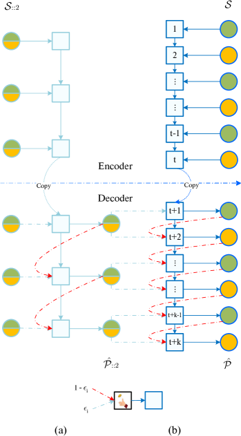
Motivated by this, we propose a TPG sampling strategy to close the gap between training and inference. First, we subsample the sequence into two subsequences by separating the odd and even indexes (see Fig. 1, green colour represents the odd index inputs and orange represents the even). The idea is to start training a simple model $\mathcal{M}_{1}(\mathrm{Encoder}(\mathcal{S}_{::2}),\theta)$ that takes the odd or even index sequence denoted as $\mathcal{S}_{::2}$. The benefit of this approach is that the sequence length is cut to half to the original length, which is much easier for both the encoder and decoder to learn. Moreover, model $\mathcal{M}_{1}$ is trained with Scheduled Sampling as in Equation 1, then the decoder input of model $\mathcal{M}_{1}$ is used as a sampling source for model $\mathcal{M}_{2}$ during the transition phase. This brings another advantage that the model is not only able to explore the differences between training and inference from itself but also the intermediate model trained with larger time scales. The detailed transition process is described as follows:

$$\begin{array}[]{l}{\forall~{}k,1\leq k\leq K,}\\ {\hat{\mathcal{X}}_{t+\frac{k}{2}::2}\sim\mathcal{M}_{1}\left(\mathrm{Encoder}_{1}(\mathcal{S}_{::2}),\tilde{\mathcal{X}}_{t+1:t+\frac{k}{2}::2};\theta_{1}\right),}\\ {\hat{\mathcal{X}}_{t+k}\sim\mathcal{M}_{2}\left(\mathrm{Encoder}_{2}(\mathcal{S}),\tilde{\mathcal{X}}_{t+1:t+k};\theta_{2}\right),}\\ {\tau_{t+k+1}\sim\mathrm{Bernoulli}\left(1,\epsilon_{i}\right)},\\ {\tilde{\mathcal{X}}_{t+k+1}=\left(1-\tau_{t+k+1}\right)\hat{\mathcal{X}}_{t+k}+\tau_{t+k+1}\tilde{\mathcal{X}}_{t+\frac{k}{2}::2}.\par}\end{array}$$ (2)

Here, $\mathcal{X}_{{t}+\frac{k}{2}::2}$ denotes decoder inputs from model $\mathcal{M}_{1}$ of the corresponding index of model $\mathcal{M}_{2}$. Similar to Scheduled Sampling, $\epsilon_{i}$ is the probability that follows the Bernoulli distribution that controls whether $\tilde{\mathcal{X}}_{t+k+1}$ samples are from the previous output $\hat{\mathcal{X}}_{t+k}$ or $\tilde{\mathcal{X}}_{{t}+\frac{k}{2}::2}$ of $\mathcal{M}_{1}$. When $\epsilon_{i}=1$, $\tilde{\mathcal{X}}_{t+k+1}=\hat{\mathcal{X}}_{t+k}$. During the transition from $\mathcal{M}_{1}$ to $\mathcal{M}_{2}$, we decrease $\epsilon_{i}$ from 1 to 0. When $\epsilon_{i}=0$, then model $\mathcal{M}_{2}$ gets solely trained conditioned on its previous output.

Although our proposed TPG Sampling share some similarities to Scheduled Sampling, there are two key differences. First, TPG closes the gap between training and inference not only from exploring the bias but also corrects the errors caused by the bias by learning the intermediate model of large time scale. Second, we careful design a decaying strategy to work with TPG which is introduced in the next section, our experiments show significant improvements.

2.3 Decay Strategy

Scheduled Sampling decreases $\epsilon_{i}$ during the transition period by the inverse sigmoid function as follows:

$$\epsilon_{i}=\frac{\lambda}{\lambda+\exp(i/\lambda)}$$ (3)

where $i$ is the current global batch number, $\lambda$ is the parameter setting to control the deceasing speed of $\epsilon_{i}$ and therefore the convergence speed. Here, the whole sequence shares the same probability to replace ground-truth with output generated by model itself, noted $\epsilon_{i}$ towards 0 the greater probability is. However, during our experiment we observed that STSF model converges from the begin of the sequence. Replacing ground-truth with system generated output for the begin of the sequence increases the convergence difficulty of the whole training process. Therefore, we propose a decay strategy that takes the current index of the sequence into account when calculating the probability as described as follows:

$$\epsilon_{i}^{v}=\frac{\lambda}{\lambda+\exp(i\times\log(\upsilon)/\lambda)}$$ (4)

where $\upsilon$ is the current index of the sequence starting from 2. Therefore, later index input has a bigger probability where ground-truth values are replaced than the earlier input at the beginning of the training process. This helps the convergence of training by keeping previous input as ground truth. However, $\epsilon_{i}^{v}$ from different indexes will become smaller and eventually to zero due to the exponential grow as towards to the end of the training, which is desire because we want all ground truth to be replaced by model generated outputs when the training is finished.

3 Weather Forecasting Experiments

To evaluate advances of our TPG sampling, we first conducted experiments on a weather forecasting task. Weather forecasting is a typical STSF task that brings many benefits to people’s everyday life as well as agriculture and many more. Experimental results show our method outperforms several baseline methods as well as the basic Seq2Seq with Scheduled Sampling.

3.1 Dataset

	t2m		rh2m		w10m
	RMSE	MAE	RMSE	MAE	RMSE	MAE
NWP	2.939	2.249	18.322	13.211	1.813	1.327
ARIMA	3.453	2.564	18.887	14.163	2.436	1.675
Seq2Seq ${}_{\scaleto{180}{2pt}}$ without sampling	3.149	2.393	16.230	11.712	1.437	1.032
Seq2Seq ${}_{\scaleto{90}{2pt}}$ + Scheduled Sampling	2.828	2.173	16.023	11.428	1.380	0.962
Seq2Seq ${}_{\scaleto{180}{2pt}}$ + Scheduled Sampling	3.080	2.334	14.180	10.254	1.417	1.035
TPG ${}_{\scaleto{\mathcal{M}_{1}}{2.5pt}}$	3.006	2.379	16.639	12.197	2.211	1.360
TPG	2.611	1.984	14.994	10.623	1.328	0.914

Table 1: Experimental results based on the test set from 01-06-2018 to 28-08-2018. Smaller number indicates smaller prediction errors.

Figure 2: Test set loss comparison during training.

AI Challenger weather forecasting is an online competition , and the goal is to predict air temperature at 2 meter (t2m), relative humidity at 2 meter (rh2m) and wind speed at 10 meter (w10m) across 10 weather stations in Beijing city. This dataset contains historic observations from 01-03-2015 to 30-10-2018. We use 01-03-2015 to 31-05-2018 for our training set, 01-06-2018 to 28-08-2018 for the test set, and 29-08-2018 to 30-10-2018 for validation purpose. Each node contains 9 measurements including t2m, rh2m, w10m and 6 others, as well as 37 other predictions which are generated by the Numerical Weather Prediction (NWP).

3.2 Implementation

3.2.1 Seq2Seq

As mentioned previously, we have 10 weather stations, each station contains observations of 9 different measurements. It is the challenge to model correlations between stations as well as correlations between different measurements. For example, wind speed and air temperature have strong correlations. In fact. every measurement could have impact on each other, however it is non-obvious but highly dynamic. As stated in the previous section, our approach is based on Seq2Seq which is capable of modeling such correlations with its encoder and decoder architecture. First, we use a LSTM encoder taking an input $\mathcal{S}\in\mathbb{R}^{T\times 10\times 9}$ which produces a feature vector $\mathbf{h}\in\mathbb{R}^{C}$. Here, $T$ is a hyper-parameter to specify the sequence length we use for feature encoding, 10 is the total number of stations, and 9 means we use all 9 measurements for feature learning. This process is called feature extraction or feature learning. During the computation of LSTM encoder for each time step, the linear transformation operation takes account of 9 measurements of 10 stations. The overall feature of all time steps will then be encoded into one vector space $\mathbf{h}$. Then such feature vector $\mathbf{h}$ will be decoded by a LSTM decoder to produce an output $\hat{\mathcal{S}}\in\mathbb{R}^{37\times 10\times 9}$ which is the following 37 hours prediction of 9 measurements. Note that, we are only predicting t2m, rh2m and w10m. Therefore, we follow a fully-connected layer to output the final prediction $\hat{\mathcal{P}}\in\mathbb{R}^{37\times 10\times 3}=\hat{\mathcal{S}}\mathbf{W}_{s}+\mathbf{b}_{s}$.

3.2.2 TPG

We extend the base Seq2Seq model with our proposed TPG sampling. To be more specific, the source sequence of length 37 is separated half into odd index and even index sequences of length 19 and 18, respectively. Such sequences are then used for the initial training of model $\mathcal{M}_{1}$. We turn the network with different settings of $\lambda_{1}$ and $\lambda_{2}$ and report comparative results to see the impact of different settings in Section 3.3.

3.2.3 Loss Function

We divide the loss function into three parts:

$$\mathcal{L}=\mathrm{MSE}_{t2m}+\mathrm{MSE}_{rh2m}+\mathrm{MSE}_{w10m},$$ (5)

where MSE denotes mean squared error: $\mathrm{MSE}=\frac{1}{n}\sum_{i=1}^{n}\left(\mathbf{X}_{i}-\hat{\mathbf{X}}_{i}\right)^{2}$. During training, $\mathcal{L}$ is optimised jointly by BPTT [26] with Adam optimiser [10].

3.2.4 Parameter Settings

For encoder and decoder, we choose a dimension $C=90$ for LSTM whilst for encoder, $T$ is set to 96 which means we use 4 days make up of 96 hours historic observations to predict the next 37 hours. For TPG, $\lambda=3000$ for weather forecasting and $\lambda=1000$ for Moving MNIST++. Learning rate for Adam is set to $1e^{-2}$.

3.2.5 Experiment Environment

We implement our model using Tensorflow 1.12, a well known deep learning library developed by Google. Our model is trained and evaluated on a server with Nvidia V100 GPU and Intel(R) Xeon(R) Gold 5118 CPU @ 2.30GHz (24 cores).

3.3 Overall Evaluation

3.3.1 Evaluation Matrix

We report experimental results on each measurement for the test set using Root Mean Squared Error (RMSE) and Mean Absolute Error (MAE):

$$\mathrm{RMSE}=\sqrt{\frac{1}{n}\sum_{i=1}^{n}\left(\mathbf{X}_{i}-\hat{\mathbf{X}}_{i}\right)^{2}}.$$ (6)

$$\mathrm{MAE}=\frac{1}{n}{\sum_{i=1}^{n}\left|\mathbf{X}_{i}-\hat{\mathbf{X}}_{i}\right|}.$$ (7)

Here, $n$ is the number of prediction time steps times the number of locations.

(a) t2m predictions

(b) rh2m predictions

(c) w10m predictions

Figure 3: Prediction visualisations (based on 30-08-2018) of air temperature (t2m), relative humidity (rh2m) and wind speed (w10m). TPG predictions have less outliers and have more accurate long term predictions.

(a) Test set loss during training

(b) Moving MNIST prediction visualisations during training.

Figure 4: A visualisation of training progress: (4(a)) shows our proposed TPG converges faster during training; (4(b)) shows our proposed TPG trains long range predictions faster and have more accurate long range predictions.

3.3.2 Baselines

NWP: Numerical Weather Prediction [13] uses mathematical models of the atmosphere and oceans to predict the weather based on current weather conditions.

ARIMA: Auto-Regressive Integrated Moving Average is the most common baseline method for time series predictions [3]. Model is trained individually by each station.

Seq2Seq ₁₈₀ without sampling: Basic Seq2Seq model with the LSTM dimension is set to 180. Other parameters are set the same as TPG model.

Seq2Seq ₉₀ + Scheduled Sampling: Basic Seq2Seq model with Scheduled Sampling of the LSTM dimension is set to 90. Other parameters are set the same as TPG model.

Seq2Seq ₁₈₀ + Scheduled Sampling: Basic Seq2Seq model with Scheduled Sampling of the LSTM dimension is set to 180. Other parameters are set the same as TPG model.

TPG ${}_{\mathcal{M}_{1}}$: Proposed TPG model with $\lambda$ is set to 500, results reported based on the intermediate model $\mathcal{M}_{1}$.

TPG: Proposed TPG model with $\lambda$ is set to 500, results reported based on the final model $\mathcal{M}_{2}$.

Note that all deep learning based models are trained with the same parameter settings otherwise stated above. Models are trained with training set, the best models are chosen which demonstrate the best performance based on the validation set, and experimental results are reported based on the test set.

3.3.3 Performance Evaluation

We compare our TPG to the baselines listed above including the tradition mathematical model NWP, and machine learning based approaches. Table 1 shows a summary of experimental results based on two evaluation matrices. It clearly demonstrates that our TPG outperforms all baselines for three measurements under study.

First, Seq2Seq based models outperform traditional approaches including NWP and ARIMA. Seq2Seq based models utilise the LSTM encoders and decoder which effectively model the spatio-temporal dynamics. To be more specific, Seq2Seq ₉₀ performs better than Seq2Seq ₁₈₀ in overall, but in particular for t2m and w10m.

Second, Table 1 also shows the Seq2Seq model trained with Scheduled Sampling performs better than Seq2Seq without sampling which shows Scheduled Sampling improves STSF. Our proposed TPG sampling continue to improve the effectiveness of bridging the gap between training and inference.

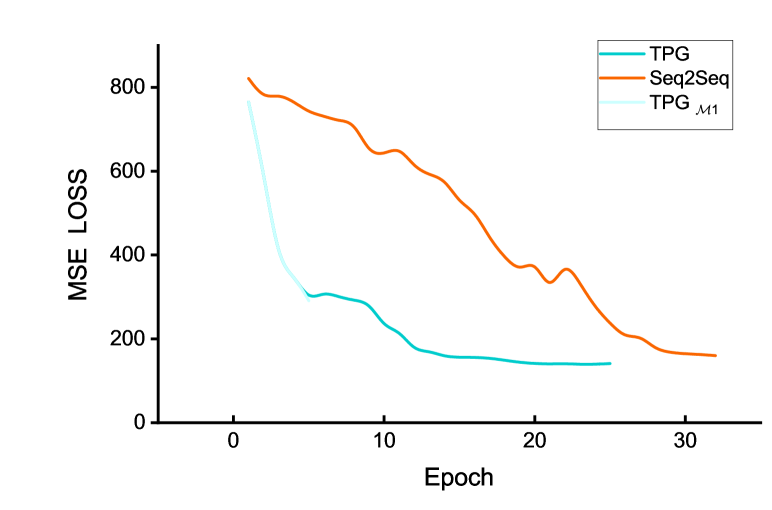
Third, our proposed TPG model outperforms base Seq2Seq models. The test of significance in terms of both accuracy measures shows that TPG significantly improves Seq2Seq ₉₀. As shown in Fig. 2, our proposed TPG model converges significantly faster than basic Seq2Seq models. The red line represents the test loss of Seq2Seq model, whilst the light blue line represents the test loss of model $\mathcal{M}_{1}$, and the dark blue line represents the test loss of model $\mathcal{M}_{2}$. Benefits from shorter sequence length, model $\mathcal{M}_{1}$ quickly converges compared to original Seq2Seq. Resulting in the second stage of training model $\mathcal{M}_{2}$, $\mathcal{M}_{2}$ shows faster convergence as well as better final performance.

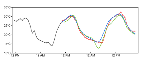
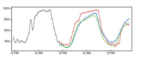
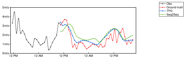
To sum up, our proposed TPG archives the best overall performance. To be specific, TPG converges much faster during training due to the progressive growing training mechanism. Prediction examples also show that TPG predictions are more reliable on the outlier predictions and the long range predictions than baseline approaches and Scheduled Sampling.

4 Moving MNIST Experiments

The weather forecasting dataset shows the outperforming performance of our proposed TPG model on a vector like dataset. In order to further evaluate the usability and applicability of our proposed method on image-like spatio-temporal sequential datasets, we further conduct experiments on the Moving MNIST dataset [20].

4.1 Dataset

The Moving MNIST dataset is originally for evaluating video (a series of sequential images) prediction performance, since then it becomes one of the most common spatio-temporal sequence prediction benchmarks [17, 25, 24]. We generate a series of image sequences containing two moving handwritten digits with different moving speed and velocity. In addition to the typical setup, we extend the sequence length to 60: 30 for the input sequence and another 30 for prediction. We generate 10,000 sequences for training, 3,000 for validation and 5,000 for testing. Experimental results are reported based on the test dataset.

4.2 Implementation

4.2.1 Seq2Seq

We use open source code provided by PredRNN++ [24] for our base Seq2Seq model for images. PredRNN++ is a strong baseline for video frame prediction which is based on Seq2Seq with a custom RNN cell, called Casual LSTM and a GHU unit.

4.2.2 TPG

Then we extend the baseline Seq2Seq model with our proposed TPG. We choose $\lambda=3000$ and we train the model for 50000 iterations.

4.3 Overall Evaluation

4.3.1 Evaluation Matrix

We report results based on two matrices: per-frame Structural Similarity Index Measure (SSIM) [30] and MSE. Larger SSIM scores indicate greater similarities between the ground-truth and prediction whilst smaller MSE values indicate smaller prediction errors.

4.3.2 Baselines

We compare the performance of our approach against several baseline methods as in PredRNN++ [24] including ConvLSTM [17], TrajGRU [18], CDNA [6], DFN [5], VPN [9] and PredRNN [25].

	SSIM $\uparrow$	MSE $\downarrow$
ConvLSTM [17]	0.597	156.2
TrajGRU [18]	0.588	163.0
CDNA [6]	0.609	142.3
DFN [5]	0.601	149.5
VPN [9]	0.620	129.6
PredRNN [25]	0.645	112.2
PredRNN++ without sampling	0.733	91.10
PredRNN++ with SS [24]	0.769	87.74
TPG	0.811	85.41

Table 2: Experimental results of 30 time steps prediction: results reported for per frame. Baselines reported as in PredRNN++ [24].

4.3.3 Performance Evaluation

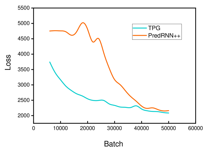
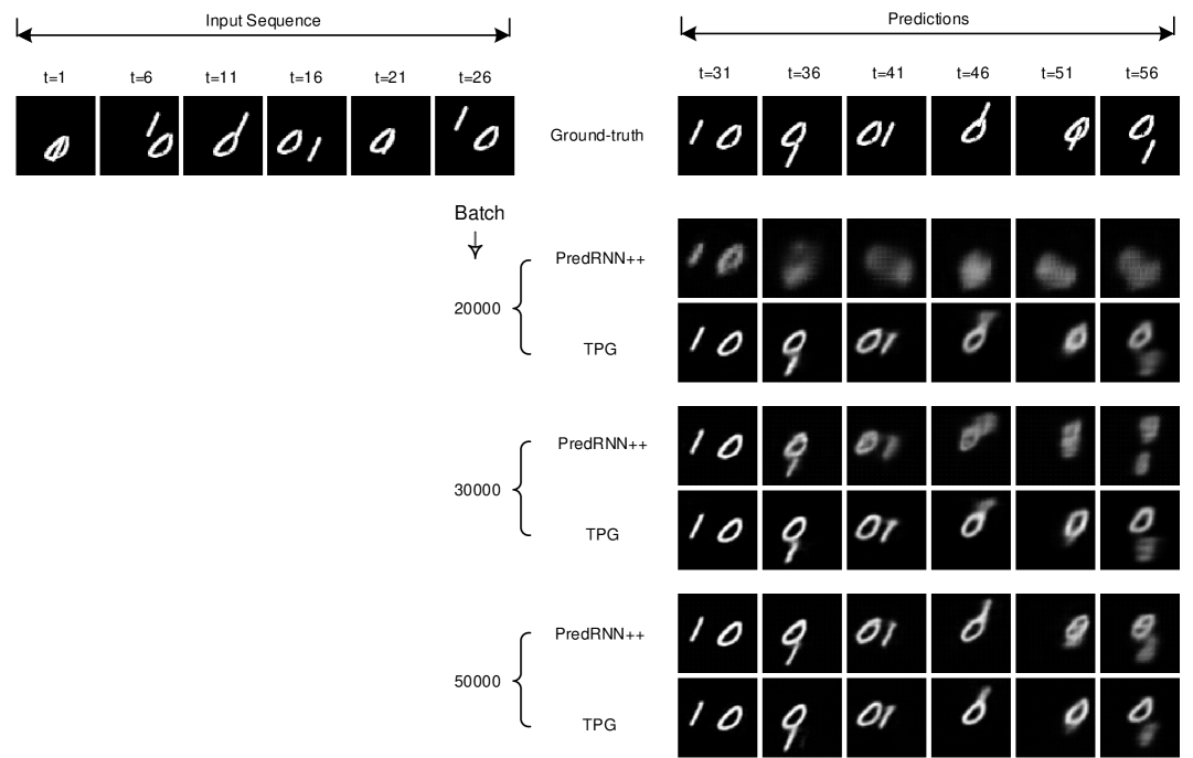
Table 2 shows a summary of experimental results with regard to the two evaluation matrices. It clearly demonstrates that our TPG outperforms all baselines reported in PredRNN++ [24]. Specifically, TPG achieves the best SSIM of 0.811 and MSE of 85.41 per frame. Moreover, Fig. 4 shows the training progress. From Fig. 4(a), we can see our proposed TPG converges much faster and smoother than other baselines. Also from prediction visualisations of Fig. 4(b) we can see our proposed TPG has more accurate long term predictions. Specifically, at batch 20000, moving hand-written digits start to be recognisable at time step 41, whereas predictions of PredRNN++ are still blurry. This could be because with the curriculum of model $\mathcal{M}_{1}$, $\mathcal{M}_{2}$ can learn longer ranges as well as higher order dynamics, whereas in regular Seq2Seq, a later time step has to wait for the earlier time step to converge first due to the nature of RNN.

5 Related Work

5.1 STSF with RNN

Spatio-temporal sequence forecasting is a well studied research topic, and it is a part of time series prediction topic. In the literature, traditional machine learning based methods including Support Vector Machine (SVM) [16], Gaussian Process (GP)[7] and Auto-Regressive Integrated Moving Average (ARIMA) [3] have been proposed to deal with this problem.

With recent advances in deep learning models in various domains, the research focus of spatio-temporal sequence forecasting has been redirected to deep models. For example, Shi et al. [19] proposed a Convolutional LSTM Recurrent Neural Network (RNN) for precipitation nowcasting. The main contribution of their work is that it models spatial correlations between two neighbouring time steps by replacing the linear transformation of LSTM with 2D-CNN, which results in more compact spatial modelling and better performance. Zhang et al. [29] proposed deep spatio-temporal residual networks to handle the citywide crowd flow prediction problem. In their work, temporal closeness, period and trends properties of crowded traffic, as well as external factors such as weather and events are considered and modelled by a fusion network. Similarly, Chen et al. [4] employed a 3D-CNN network to approach the problem. All these studies model the spatio-temporal data at a certain timestamp as an image-like format, each measurement at a location is treated as a pixel of an image. Therefore, modeling series of spatio-temporal data is the same as modeling videos (a series of images with a regular time interval). Forecasting a spatio-temporal sequence is highly relevant to the problem of video frame prediction. Wang et al. proposed PredRNN [25] and its following work PredRNN++ [24] to solve the video frame prediction problem. Their work is based on Seq2Seq with a custom RNN cell called Casual LSTM and a GHU unit.

Modeling a spatio-temporal sequence as a video-like format requires a rich collection of data in a variety of coordinate locations, also coordinate locations have to be a grid like format to be compatible as in the city crowd flow prediction. However, not all datasets satisfy these constraints. Another approach is to model spatio-temporal data as a vector, where each measurement of a location is a scalar of a row or column. For example, Ghaderi et al. [8] proposed a LSTM-based model to predict wind speed across 57 measurement locations. Wang et al. [23] proposed a deep uncertainty Seq2Seq model to predict weather for 10 weather stations across Beijing City. Yi et al. [27] proposed a DeepAir model which consists of a spatial transformation component and a deep distributed fusion network to predict air quality. In another work, Liang et al. [12] proposed a multi-level attention Seq2Seq model called GeoMAN to model dynamics of spatio-temporal dependencies. All these studies above reveal spatio-temporal correlations are difficult to model, but are crucial for spatial-temporal predictions.

5.2 Curriculum Learning Strategy

Venktrman et al. [22] proposed a Data As Demonstrator (DAD) model to improve multi-step prediction by feeding paired ground-truth and predicted word to the next step. The gap between single step prediction error and multi-step error in their work is similar to the gap between training and inference in our work. Bendigo et al. [1] further improve the idea by a Curriculum Learning [2] based approach to close the gap between training and inference by sampling previous ground-truth and previously predicted context by a changing probability.

6 Conclusions and Future Work

In this paper, we propose TPG Sampling to bridge the gap between training and inference for Seq2Seq based STSF systems. By transforming the training process from a fully-supervised manner which utilises all available previous ground-truth to a less-supervised manner which replaces the ground-truth contexts with generated predictions. We also sample the target sequence from midway outputs from the intermediate model trained with bigger timescales with a carefully designed decaying strategy. Experiments on two datasets demonstrate that our proposed method achieves superior performance compared to all baseline methods, and show fast convergence speed as well as better long term accuracies. Two different types of datasets used in experiments prove the novelty and applicability of our proposed method.

Future studies are in two folds. First, an extensive ablation study along with a hyperparameter optimization study is required to further validate the applicability and utility of Temporal Progressive Growing Sampling. Second, we can extend the progressive idea to spatial and temporal dimensions simultaneously for spatio-temporal sequence predictive learning.

References

- [1] Samy Bengio, Oriol Vinyals, Navdeep Jaitly, and Noam Shazeer, ‘Scheduled sampling for sequence prediction with recurrent neural networks’, in Proceedings of the 28th International Conference on Neural Information Processing Systems - Volume 1, NIPS’15, pp. 1171–1179, Cambridge, MA, USA, (2015). MIT Press.
- [2] Yoshua Bengio, Jérôme Louradour, Ronan Collobert, and Jason Weston, ‘Curriculum learning’, in Proceedings of the 26th Annual International Conference on Machine Learning, ICML ’09, p. 41–48, New York, NY, USA, (2009). Association for Computing Machinery.
- [3] George Edward Pelham Box and Gwilym Jenkins, Time Series Analysis, Forecasting and Control, Holden-Day, Inc., San Francisco, CA, USA, 1990.
- [4] C. Chen, K. Li, S. G. Teo, G. Chen, X. Zou, X. Yang, R. C. Vijay, J. Feng, and Z. Zeng, ‘Exploiting spatio-temporal correlations with multiple 3d convolutional neural networks for citywide vehicle flow prediction’, in 2018 IEEE International Conference on Data Mining (ICDM), pp. 893–898, (Nov 2018).
- [5] Bert De Brabandere, Xu Jia, Tinne Tuytelaars, and Luc Van Gool, ‘Dynamic filter networks’, in Proceedings of the 30th International Conference on Neural Information Processing Systems, NIPS’16, pp. 667–675, USA, (2016). Curran Associates Inc.
- [6] Chelsea Finn, Ian Goodfellow, and Sergey Levine, ‘Unsupervised learning for physical interaction through video prediction’, in Proceedings of the 30th International Conference on Neural Information Processing Systems, NIPS’16, pp. 64–72, USA, (2016). Curran Associates Inc.
- [7] Seth R. Flaxman, Machine learning in space and time, Ph.D. dissertation, 2015.
- [8] Amir Ghaderi, Borhan M Sanandaji, and Faezeh Ghaderi, ‘Deep forecast: Deep learning-based spatio-temporal forecasting’, in The 34th International Conference on Machine Learning (ICML), Time series Workshop, (2017).
- [9] Nal Kalchbrenner, Aäron van den Oord, Karen Simonyan, Ivo Danihelka, Oriol Vinyals, Alex Graves, and Koray Kavukcuoglu, ‘Video pixel networks’, in Proceedings of the 34th International Conference on Machine Learning - Volume 70, ICML’17, pp. 1771–1779. JMLR.org, (2017).
- [10] Diederik P. Kingma and Jimmy Ba, ‘Adam: A Method for Stochastic Optimization’, arXiv e-prints, arXiv:1412.6980, (Dec 2014).
- [11] Yaguang Li, Rose Yu, Cyrus Shahabi, and Yan Liu, ‘Diffusion convolutional recurrent neural network: Data-driven traffic forecasting’, in International Conference on Learning Representations, (2018).
- [12] Yuxuan Liang, Songyu Ke, Junbo Zhang, Xiuwen Yi, and Yu Zheng, ‘Geoman: Multi-level attention networks for geo-sensory time series prediction’, in Proceedings of the Twenty-Seventh International Joint Conference on Artificial Intelligence, IJCAI-18, pp. 3428–3434. International Joint Conferences on Artificial Intelligence Organization, (7 2018).
- [13] Peter Lynch, ‘The origins of computer weather prediction and climate modeling’, J. Comput. Phys., 227(7), 3431–3444, (March 2008).
- [14] Marc’Aurelio Ranzato, Sumit Chopra, Michael Auli, and Wojciech Zaremba, ‘Sequence level training with recurrent neural networks’, in 4th International Conference on Learning Representations, ICLR 2016, San Juan, Puerto Rico, May 2-4, 2016, Conference Track Proceedings, (2016).
- [15] D. Salinas, V. Flunkert, and J. Gasthaus, ‘DeepAR: Probabilistic Forecasting with Autoregressive Recurrent Networks’, arXiv e-prints, (April 2017).
- [16] N. I. Sapankevych and R. Sankar, ‘Time series prediction using support vector machines: A survey’, IEEE Computational Intelligence Magazine, 4(2), 24–38, (May 2009).
- [17] Xingjian Shi, Zhourong Chen, Hao Wang, Dit-Yan Yeung, Wai-kin Wong, and Wang-chun Woo, ‘Convolutional lstm network: A machine learning approach for precipitation nowcasting’, in Proceedings of the 28th International Conference on Neural Information Processing Systems - Volume 1, NIPS’15, pp. 802–810, Cambridge, MA, USA, (2015). MIT Press.
- [18] Xingjian Shi, Zhihan Gao, Leonard Lausen, Hao Wang, Dit-Yan Yeung, Wai-kin Wong, and Wang-chun Woo, ‘Deep learning for precipitation nowcasting: a benchmark and a new model’, in Advances in Neural Information Processing Systems, (2017).
- [19] Xingjian Shi and Dit-Yan Yeung, ‘Machine Learning for Spatiotemporal Sequence Forecasting: A Survey’, arXiv e-prints, arXiv:1808.06865, (Aug 2018).
- [20] Nitish Srivastava, Elman Mansimov, and Ruslan Salakhutdinov, ‘Unsupervised learning of video representations using lstms’, in Proceedings of the 32Nd International Conference on International Conference on Machine Learning - Volume 37, ICML’15, pp. 843–852. JMLR.org, (2015).
- [21] Ilya Sutskever, Oriol Vinyals, and Quoc V Le, ‘Sequence to sequence learning with neural networks’, in Advances in Neural Information Processing Systems 27, eds., Z. Ghahramani, M. Welling, C. Cortes, N. D. Lawrence, and K. Q. Weinberger, 3104–3112, Curran Associates, Inc., (2014).
- [22] Arun Venkatraman, Martial Hebert, and J. Andrew Bagnell, ‘Improving multi-step prediction of learned time series models’, in Proceedings of the Twenty-Ninth AAAI Conference on Artificial Intelligence, AAAI’15, pp. 3024–3030. AAAI Press, (2015).
- [23] Bin Wang, Zheng Yan, Huaishao Luo, Tianrui Li, Jie Lu, and Guangquan Zhang, ‘Deep uncertainty learning: A machine learning approach for weather forecasting’, CoRR, abs/1812.09467, (2018).
- [24] Yunbo Wang, Zhifeng Gao, Mingsheng Long, Jianmin Wang, and Philip S Yu, ‘PredRNN++: Towards a resolution of the deep-in-time dilemma in spatiotemporal predictive learning’, in Proceedings of the 35th International Conference on Machine Learning, eds., Jennifer Dy and Andreas Krause, volume 80 of Proceedings of Machine Learning Research, pp. 5123–5132, Stockholmsmässan, Stockholm Sweden, (10–15 Jul 2018). PMLR.
- [25] Yunbo Wang, Mingsheng Long, Jianmin Wang, Zhifeng Gao, and Philip S Yu, ‘Predrnn: Recurrent neural networks for predictive learning using spatiotemporal lstms’, in Advances in Neural Information Processing Systems 30, eds., I. Guyon, U. V. Luxburg, S. Bengio, H. Wallach, R. Fergus, S. Vishwanathan, and R. Garnett, 879–888, Curran Associates, Inc., (2017).
- [26] P. J. Werbos, ‘Backpropagation through time: what it does and how to do it’, Proceedings of the IEEE, 78(10), 1550–1560, (Oct 1990).
- [27] Xiuwen Yi, Junbo Zhang, Zhaoyuan Wang, Tianrui Li, and Yu Zheng, ‘Deep distributed fusion network for air quality prediction’, in Proceedings of the 24th ACM SIGKDD International Conference on Knowledge Discovery & Data Mining, KDD ’18, pp. 965–973, New York, NY, USA, (2018). ACM.
- [28] Rose Yu, Stephan Zheng, Anima Anandkumar, and Yisong Yue, ‘Long-term Forecasting using Tensor-Train RNNs’, arXiv e-prints, arXiv:1711.00073, (Oct 2017).
- [29] Junbo Zhang, Yu Zheng, Dekang Qi, Ruiyuan Li, Xiuwen Yi, and Tianrui Li, ‘Predicting citywide crowd flows using deep spatio-temporal residual networks’, Artificial Intelligence, 259, 147 – 166, (2018).
- [30] Zhou Wang, A. C. Bovik, H. R. Sheikh, and E. P. Simoncelli, ‘Image quality assessment: from error visibility to structural similarity’, IEEE Transactions on Image Processing, 13(4), 600–612, (April 2004).