TAIP: an anytime algorithm for allocating student teams to internship programs

Abstract.

In scenarios that require teamwork, we usually have at hand a variety of specific tasks, for which we need to form a team in order to carry out each one. Here we target the problem of matching teams with tasks within the context of education, and specifically in the context of forming teams of students and allocating them to internship programs. First we provide a formalization of the Team Allocation for Internship Programs Problem, and show the computational hardness of solving it optimally. Thereafter, we propose TAIP, a heuristic algorithm that generates an initial team allocation which later on attempts to improve in an iterative process. Moreover, we conduct a systematic evaluation to show that TAIP reaches optimality, and outperforms CPLEX in terms of time.

1. Introduction

In the context of education, it is increasingly common that students spend some time doing practical work in a company as part of their curriculum. This work is sometimes remunerated: companies benefit from this program as they get motivated students that will work for reduced wages, and students benefit from a first contact with the labour market. It has been found that the employability of students at the end of their studies increases thanks to these internships. Nowadays, education authorities match students with companies mostly by hand. This paper formalises this matching process as a combinatorial optimization problem, proposes some heuristic algorithms and studies their computational complexity.

Team formation with respect to skills/expertise is a well studied topic of interest within the AI and MAS community Andrejczuk et al. (2018).  Anagnostopoulos et al. (2012) tackle the problem of team formation considering skills, communication costs, and tasks that progressively arrive in time. In the same direction, Kargar et al. (2012) propose a heuristic algorithm for forming one team of experts for a specific task.  Crawford et al. (2016) propose several heuristic algorithms for forming a single robust team in order to compete a given set of tasks. The authors in Andrejczuk et al. (2019) target the problem of partitioning a group of individuals into equal-sized teams so that each one will resolve the same task. Here we consider the problem of allocating individuals into teams of different sizes in order to resolve different tasks. In fact, our problem can be viewed as a generalization of Andrejczuk et al. (2019).

In this work, we present and formalise an actual-world problem, the so-called Team Allocation for Internship Programs (TAIPP). We characterise the complexity of the TAIPP and the search space that an algorithm that solves it must cope with. We propose how to encode the TAIPP as a linear program so that it can be solved by a general purpose LP solver. Furthermore, we propose a novel, anytime heuristic algorithm that exploits the structure of the TAIPP. As we will show, our proposed algorithm outperforms the general purpose optimizer IBM CPLEX in terms of time: it always reaches the optimal solution at least 55% faster than CPLEX, and reaches a quality of 80% in less than 20% of the time we need to construct the input for CPLEX.

As such, in what follows, in Sec 2 we formally describe the TAIPP, provide formal definitions of the problem’s components, and study the complexity of the problem. In Sec 3 we provide the encoding for a linear program solver. In Sec 4 we propose our heuristic algorithm; while in Sec 5 we conduct a systematic evaluation and show the effectiveness of our algorithm.

2. Problem Formalization

In this section we present the individual components of the problem, discuss their intuition, and provide formal definitions. We begin with the formalization of internship programs and students, along with a thorough discussion on the essential notion of competencies. Then we proceed on presenting our notion of competence coverage, and show how to compute it.

2.1. Basic elements of the allocation problem

An internship program is characterised by a set of requirements on student competencies and team size constraints. For instance, think of an internship program in a computer tech company: there are 4 competence requirements (a) machine learning principles, (b) coding in python, (c) web development, and (d) fluency in Spanish language, while the required team size is 3 members; as such, for this program we need a team of three students that as a team possesses the four required competencies.

In general we can have a large variety of other constraints, such as temporal or spatial constraints, i.e., when and where the internship can be realised. However, within the scope of this paper, we only focus on team size constraints. The required competencies are often accompanied by their level and importance. Formally, an internship program $p$ is a tuple $\langle C,l,w,m\rangle$, where $C$ is the set of required competencies, $l:C\to\mathbb{R}^{+}\cup\{0\}$ is a required competence level function, $w:C\to(0,1]$ is a function that weighs the importance of competences, and $m\in\mathbb{N}_{+}$ is the team size required. The set of all internship programs is denoted with $P$, with $|P|=M$.

A student is characterised by their competencies, and their competence levels. Formally, a student $s$ is represented as a tuple $\langle C,l\rangle$, where $C$ is the set of already acquired competencies, and $l:C\to\mathbb{R}_{+}\cup\{0\}$ is a competence level function, and hence $l(c)$ is the student’s competence level for competence $c$. The set of all students is denoted with $S$, with $|S|=N$. Given $p\in P$, we denote the set of all size-compliant teams for $p$ as $\mathcal{K}_{p}=\{K\subseteq S:|K|=m_{p}\}$.

But size is not enough, we need that the members of a team are suitable for the competencies requested by a company. We assume that there is a predefined ontology that provides a fixed and finite set of competencies $C$ along with relations among them. We further assume that the ontology is a tree graph, where children denote more specific competencies than those of their parents. Formally, an ontology is a tuple $o=\langle C,E\rangle$ with $C$ being the competencies-nodes and $E$ the edges. The metric over ontologies that we will use next is the semantic similarity. The semantic similarity is given by

$$\mathrm{sim}(c_{1},c_{2})=\begin{cases}1,&\text{if }l=0\\ e^{-\lambda l}\frac{e^{\kappa h}-e^{-\kappa h}}{e^{\kappa h}+e^{-\kappa h}},&\text{otherwise}\end{cases}$$ (1)

where $l$ is the shortest path in the tree between $c_{1}$ and $c_{2}$, $h$ is the depth of the deepest competence subsuming both $c_{1}$ and $c_{2}$, and $\kappa,\lambda\in[1,2]$ are parameters regulating the influence of $l$ and $h$ to the similarity metric. This is a variation of the metric introduced in Li et al. (2003), which guarantees the reflexive property of similarity, that is, a node is maximally similar to itself, independently of its depth. In other words, nodes at zero distance ($l=0$) have maximum similarity. Similarly to Osman et al. (2014), the semantic similarity between two competence lies in $[0,1]$.

2.2. Computing competence coverage for students and teams

In order to evaluate how well a student fits with an internship we need some notion of coverage for each competence required by an internship by the actual competencies of a student. Thus, we define the student coverage of competence $c$ by a set of competencies $A\subseteq C$ as $\mathrm{cvg}(c,A)=\max_{c^{\prime}\in A}\{\mathrm{sim}(c,c^{\prime})\}$.

And then, naturally, given a program $p$ with required competencies $C_{p}$ and a student $s$ with acquired competencies $C_{s}$ the competence coverage of program $p$ by student $s$ is:

$$\mathrm{cvg}(s,C_{p})=\prod_{c\in C_{p}}\mathrm{cvg}(c,C_{s})=\prod_{c\in C_{p}}\max_{c^{\prime}\in C_{s}}\{\mathrm{sim}(c,c^{\prime})\}$$ (2)

Moving now from a single student $s\in S$ to a team of students $K\subseteq S$, we need first to solve a competence assignment problem. That is, we need to assign to each student $s\in K$ a subset of competencies of $C_{p}$, and assume that student $s$ is responsible for (in charge of) their assigned competencies. According to Andrejczuk et al. (2019) we have that:

Definition (Competence Assignment Function (CAF)).

Given a program $p\in P$, and a team of students $K\subseteq S$, a competence assignment $\eta_{p}^{K}$ is a function $\eta_{p}^{K}:K\to 2^{C_{p}}$, satisfying $C_{p}=\bigcup_{s\in K}\eta_{p}^{K}(s)$.

The set of competence assignments functions for program $p$ and team $K$ is noted by $\Theta_{p}^{K}$. The inverse function $\eta_{p}^{K\ -1}:C_{p}\to 2^{K}$ provides us with the set of students in $K$ that are assigned to competence $c\in C_{p}$.

However, not all competence assignments are equally accepted. For example, consider a program $p$ (with $C_{p}=\{c_{1},c_{2},c_{3},c_{4},c_{5}\}$), and a team $K=\{s_{1},s_{2},s_{3}\}$. An assignment $\eta_{p}^{K}$ such that $\eta_{p}^{K}(s_{1})=C_{p}$ and $\eta_{p}^{K}(s_{2})=\eta_{p}^{K}(s_{3})=\emptyset$ seems to be unfair—assigning all competencies as student $s_{1}$’s responsibility—,while assignment $\tilde{\eta}_{p}^{K}$ such that $\tilde{\eta}_{p}^{K}(s_{1})=\{c_{1},c_{3}\}$, $\tilde{\eta}_{p}^{K}(s_{2})=\{c_{2},c_{5}\}$ and $\tilde{\eta}_{p}^{K}(s_{3})=\{c_{4}\}$ is more fair, in terms of allocating responsibilities. In the setting of internship programs, we prefer assignments such that all students are actively participating, i.e., assignments such that $\eta_{p}^{K}(s)\neq\emptyset$ for each student $s$ (the so-called inclusive assignments in  Andrejczuk (2018)). At the same time, we would prefer not to ‘overload’ a few students with excessive responsibilities, but selecting fair competence assignments. This is captured by the following definition:

Definition (Fair Competence Assignment Function (FCAF)).

Given a program $p$, and a team of students $K\subseteq S$, a fair competence assignment $\eta_{p}^{K}$ is a function $\eta_{p}^{K}:K\to 2^{C_{p}}$, satisfying $C_{p}=\bigcup_{s\in K}\eta_{p}^{K}(s)$, $1\leq|\eta_{p}^{K}(s)|\leq\lceil\frac{|C_{p}|}{|K|}\rceil\ \forall s\in K$, and $1\leq|\eta_{p}^{K\ -1}(c)|\leq\lfloor\frac{|K|}{|C_{p}|}\rfloor+1$.

Now, given a competence assignment $\eta_{p}^{K}$, we define the competence proximity of a student $s$ wrt a program $p$. To do so we take into consideration the importance of each competence and the students coverage of the assigned competencies. In the competence proximity we want to encode the following scenarios:

• the competence proximity should be as high as possible when the coverage of a competence by a student is maximum;

• the competence proximity should be as high as possible when the competence is not important;

• the competence proximity should be as low as possible when the coverage of a competence by all students is minimum.

For a competence $c\in C_{p}$ and a student $s$, we can visualise the above properties in the truth table in Table 1.

$\mathrm{cvg}(\downarrow)\setminus w(\to)$	$0$	$(0,1)$	$1$
$0$	$1$	$1$	$1$
$(0,1)$	$1$		$\sim\mathrm{cvg}$
$1$	$1$	$\sim(1-w)$	$0$

Table 1. Competence proximity truth table; $\mathrm{cvg}$ stands for $\mathrm{cvg}(c,C_{s})$, and $w$ for $w_{p}(c)$.

If we think $\mathrm{cvg}(c,C_{s})$ and $w_{p}(c)$, the importance of competence c in program p, as Boolean variables, we can interpret this table as a logical formula

$$w_{p}(c)\Rightarrow\mathrm{cvg}(c,C_{s})\equiv\big{(}1-w_{p}(c)\big{)}\vee\mathrm{cvg}(c,C_{s})$$

However, $\mathrm{cvg}(c,C_{s})$ and $w_{p}(c)$ are continuous variables in $[0,1]$, so we model the ‘or’ condition of the above logical formula as the ‘maximum’ between the two variables. As such, we define the competence proximity of a student for an internship program as:

Definition (Student’s Competence Proximity).

Given a student $s\in S$, an internship program $p\in P$, and a competence assignment $\eta_{p}$, the competence proximity of $s$ for $p$ with respect to $\eta_{p}$ is:

$$\mathrm{cp}(s,p,\eta_{p})=\prod_{c\in\eta_{p}(s)}\max\big{\{}\big{(}1-w_{p}(c)\big{)},\mathrm{cvg}(c,C_{s})\big{\}}.$$ (3)

Moving to the competence proximity of a team of students $K\subseteq S$ for program $p$, we use the Nash product of the competence proximity of the individuals in $K$ for $p$, with respect to some FCAF $\eta_{p}$. The Nash product assigns a larger value to teams where all students equally contribute to their program, rather than to teams where some students have a small contribution.

Definition (Team’s Competence Proximity).

Give a team $K$ a program $p\in P$, and a competence assignment $\eta_{p}$, the competence proximity of team $K$ for program $p$ is:

$$\mathrm{cp}(K,p,\eta_{p}^{K})=\prod_{s\in K}\mathrm{cp(s,p,\eta_{p}^{K})}.$$ (4)

For a team $K$ and a program $p$ its competence proximity varies depending on the competence assignment at hand. We define the best competence assignment as the fair one (Definition 2.2) that maximizes the competence proximity:

$$\eta_{p}^{K\ *} =\operatorname*{arg\,max}_{\eta_{p}^{K}\in\Theta_{p}^{K}}\{\mathrm{cp}\big{(}K,p,\eta_{p}^{K}\big{)}\}$$

$$=\operatorname*{arg\,max}_{\eta_{p}^{K}\in\Theta_{p}^{K}}\prod_{s\in K}\mathrm{cp(s,p,\eta_{p}^{K})}$$

$$=\operatorname*{arg\,max}_{\eta_{p}^{K}\in\Theta_{p}^{K}}\prod_{c\in\eta_{p}(s)}\max\big{\{}\big{(}1-w_{p}(c)\big{)},\mathrm{cvg}(c,C_{s})\big{\}}$$

Finding the best competence assignment is optimization problem itself. Even though the above is not a linear optimization problem, it can be easily linearized by considering the logarithm of $\mathrm{cp}\big{(}\cdot\big{)}$:

$$\eta_{p}^{K\ *} =\operatorname*{arg\,max}_{\eta_{p}^{K}\in\Theta_{p}^{K}}\{\mathrm{cp}\big{(}K,p,\eta_{p}^{K}\big{)}\}\equiv\operatorname*{arg\,max}_{\eta_{p}^{K}\in\Theta_{p}^{K}}\{\log\{\mathrm{cp}\big{(}K,p,\eta_{p}^{K}\big{)}\}\}$$

$$=\operatorname*{arg\,max}_{\eta_{p}^{K}\in\Theta_{p}^{K}}\log\Big{\{}\prod_{s\in K}\mathrm{cp(s,p,\eta_{p}^{K})}\Big{\}}=\operatorname*{arg\,max}_{\eta_{p}^{K}\in\Theta_{p}^{K}}\sum_{s\in K}\log\big{\{}\mathrm{cp(s,p,\eta_{p}^{K})}\big{\}}$$

2.3. The team allocation problem as an optimisation problem

Finding a good allocation of students to a collection of internship programs is yet another optimization problem that tries to maximize the overall competence proximity of all teams for their assigned internship program. That is, for a single program $p$, the best candidate team is the one that maximizes the competence proximity: $K^{*}=\operatorname*{arg\,max}_{K\in\mathcal{K}_{p}}\ \mathrm{cp}(K,p)$. $K^{*}$ is the best candidate when a single program is at hand. For a set of programs $P$, with $|P|>1$, we need to maximize the competence proximity of all candidate teams with their corresponding programs. Suppose we have a team assignment function $g:P\to 2^{S}$, which maps each $p\in P$ with a team of students $K\in\mathcal{K}_{p}$. We assume that for two programs $p_{1}$ and $p_{2}$ it holds that $p_{1}=p_{2}\Leftrightarrow g(p_{1})=g(p_{2})$. In the setting of matching internship programs with teams of students we should consider only team assignment functions $g$ such that $g$ assigns each student to at most one program. As such, we can define feasible team assignment functions:

Definition (Feasible Team Assignment Functions (FTAF)).

Given a set of programs $P$ and a set of students $S$, a feasible team assignment function $g\in G$ is such that for each pair of programs $p_{1},p_{2}\in P$ with $p_{1}\neq p_{2}$, it holds that $g(p_{1})\cap g(p_{2})=\emptyset$; and for all $p\in P$ it holds that $|g(p)|=m_{p}$.

The family of all feasible team assignments is denoted with $G_{\mathrm{feasible}}$. Now we are ready to formalise our team allocation problem as follows:

Definition (Team Allocation for Internship Programs Problem (TAIPP)).

Give a set of internship programs $P$, and a set of students $S$, the team allocation for internship programs problem is to select the team assignment function $g^{*}\in G$ that maximizes the overall competence proximity:

$$g^{*}=\operatorname*{arg\,max}_{g\in G_{feasible}}\ \prod_{p\in P}\mathrm{cp}\big{(}g(p),p,\eta_{p}^{g(p)\ *}\big{)}$$ (7)

The following result establishes that the TAIPP is $\mathcal{NP}-complete$ by reduction to a well-known problem in the MAS literature.

The TAIPP, with more than one program at hand, is $\mathcal{NP}-complete$.

Proof.

The problem is in $\mathcal{NP}$ since we can decide whether a given solution is feasible in polynomial time ($\mathcal{O}(\sum_{p\in P}m_{p})$). We show that the problem is $\mathcal{NP}-complete$ by using a reduction from Single Unit Auctions with XOR Constraints and Free Disposals (referred to as BCAWDP with XOR Constraints) which is shown to be $\mathcal{NP}-complete$ Sandholm et al. (2002). In the BCAWDP with XOR Constraints, the auctioneer has $N$ items to sell, the bidders place their bids $B_{i}=\langle\mathbf{b}_{i},b_{i}\rangle$ with $\mathbf{b}_{i}$ be a subset of items and $b_{i}$ the price. Between two bids can exist an XOR constraint–not necessarily to every pair of bids. The auctioneer allows free disposals, i.e., items can remain unsold. Given an instance of BCAWDP with XOR Constraints, we construct an instance of student-teams allocation to internship programs problem as follows: “For each item $i$ we create a student $s_{i}$. For each program $p_{j}$ of size $m_{p_{j}}$ we create $\binom{|S|}{m_{p_{j}}}$ different bids $B_{jk}=\langle\mathbf{b}_{jk},b_{jk}\rangle$, where $|S|$ is the number of items, $|\mathbf{b}_{jk}|=m_{p_{i}}$, and $b_{jk}=\mathrm{cp}\big{(}\mathbf{b}_{jk},p_{j},\eta_{p_{j}}^{\mathbf{b}_{jk}\ *}\big{)}$. All bids created for program $p_{j}$ are XOR-constrained bids. Moreover, each pair of bids $B_{j,k},B_{q,l}$ such that $\mathbf{b}_{jk}\cap\mathbf{b}_{ql}\neq\emptyset$ are also XOR-constrained.” Now the team allocation for internship programs problem has a feasible solution if and only if BCAWDP with XOR constraints has a solution. ∎

Typically, the winner determination problem for combinatorial auctions can be cast and solved as a linear program. Along the same lines, we propose how to solve the TAIPP by meas of LP in Sec 3. Before that, the following section characterises the search space with which an algorithm solving the TAIPP must cope.

2.4. Characterising the search space

The purpose of this section is to characterise the search space defined by the TAIPP. This amounts to quantifying the number of feasible team assignment functions in $G_{\mathrm{feasible}}$. For that, we start by splitting the programs in $P$ into $k$ buckets of programs, where the programs in the same bucket require teams of the same size. That is, we have $b_{1},\cdots,b_{k}\subseteq P$ buckets where $b_{i}\cap b_{j}=\emptyset,\ \forall i,j=1,\cdots,k$ and $\bigcup_{i=1}^{k}b_{i}=P$. For each bucket $b_{i}$ with $|b_{i}|=n_{i}$, it holds that $m_{p_{1}}=m_{p_{2}}=\cdots=m_{p_{n_{i}}}=m_{i}$ for all $p_{1},p_{2},\cdots,p_{n_{i}}\in b_{i}$; and $m_{i}\neq m_{j}$, that characterise $b_{i}$ and $b_{j}$ respectively, for any $i\neq j=1,\cdots,k$. Next, we will distinguish three cases when counting the number of feasible teams in $G_{\mathrm{feasible}}$:

• Case I : $\sum_{p\in P}m_{p}=\sum_{i=1}^{k}m_{i}\cdot|b_{i}|=N$, we have exactly as many students as required by all programs in $P$. In this case, we seek for partition functions over $P$. The space of $G_{\text{feasible}}$ is $\frac{N!}{\prod_{i=1}^{k}(m_{i}!)^{b_{i}}}$ according to Theorem 3.4.19 in Maddox (2002).

• Case II : $\sum_{p\in P}m_{p}=\sum_{i=1}^{k}m_{i}\cdot|b_{i}|<N$, we have more students than the required ones by all programs in $P$. Following the Example 3.4.20 in Maddox (2002), we assume one more bucket $b_{k+1}$ containing exactly one auxiliary program, which requires a team of size $m_{k+1}=\sum_{i=1}^{k}m_{i}\cdot|b_{i}|-N$. Now there are $|G_{\mathrm{feasible}}|=\frac{N!}{\prod_{i=1}^{k}(m_{i}!)^{b_{i}}\cdot\big{(}N-\sum_{i=1}^{k}|b_{i}|\cdot m_{i}\big{)}!}$ different feasible team assignment functions.

• Case III: $\sum_{p\in P}m_{p}=\sum_{i=1}^{k}m_{i}\cdot|b_{i}|>N$, we have less students than the required ones by all programs in $P$. In this case, first we need to introduce $cover(P,S)=\{P^{\prime}\subset P:\sum_{p\in P^{\prime}}m_{p}\leq N\wedge\not\exists\ p^{\prime}\in P-P^{\prime}:m_{p^{\prime}}\leq N-\sum_{p\in P^{\prime}}m_{p}\}$ as the set that contains all the subsets of programs $P^{\prime}\subset P$ such that $S,P^{\prime}$ leads to Case I or Case II, and by adding any $p\not\in P^{\prime}$ in $p^{\prime}$ it will lead to Case III. The number of feasible team assignment functions is:

  $$|G_{\mathrm{feasible}}|=\sum_{P^{\prime}\in cover(P,S)}\frac{N!}{\prod_{i=1}^{k}(m_{i}!)^{b_{i}}\cdot\big{(}N-\sum_{i=1}^{k}|b_{i}|\cdot m_{i}\big{)}!}$$

  where variables $k,b_{1},\cdots,b_{k}$ and $m_{1},\cdots,m_{k}$ changes according to $P^{\prime}$. The size of set $cover(P,S)$ depends on the total number of students, and the team sizes required by the programs in $P$.

Note that the number of feasible team assignment functions quickly grows with the number of programs and students, hence leading to very large search spaces.

3. Solving The TAIPP as a linear program

In what follows we show how to solve the TAIPP in Definition 2.3 as an LP. First, for each time $K\subseteq S$ and program $p\in P$, we will consider a binary decision variable $x_{K}^{p}$. The value of $x_{K}^{p}$ indicates whether team $K$ is assigned to program $p$ or not as part of the optimal solution of the TAIPP. Then, solving the TAIPP amounts to solving the following non-linear program:

$$\max\prod_{p\in P}\prod_{k\in\mathcal{K}_{p}}\Big{(}\mathrm{cp}\big{(}K,p,\eta_{p}^{K\ *}\big{)}\Big{)}^{x_{K}^{p}}$$ (8)

subject to:

$$\sum_{K\subseteq S}x_{K}^{p}\cdot\mathbbm{1}_{K\in\mathcal{K}_{p}}\leq 1 \forall p\in P$$ (9a)

$$\sum_{p\in P}\sum_{K\subseteq S}x_{K}^{p}\cdot\mathbbm{1}_{s\in K}\cdot\mathbbm{1}_{K\in\mathcal{K}_{p}}\leq 1 \forall s\in S$$ (9b)

$$x_{K}^{p}\in\{0,1\} \forall K\subseteq S,p\in P$$ (9c)

Constraint 9a ensures that a program is allocated a single team. Constraint 9b ensures that any two teams sharing some student cannot be assigned to programs at the same time. Notice that the objective function (see Eq 8) is non-linear. Nevertheless, it is easy to linearise it by maximising the logarithm of $\prod_{p\in P}\prod_{k\in\mathcal{K}_{p}}\Big{(}\mathrm{cp}\big{(}K,p,\eta_{p}^{K\ *}\big{)}\Big{)}^{x_{K}^{p}}$. Thus, solving the non-linear program above is equivalent to solving the following binary linear program:

$$\operatorname{max}\sum_{p\in P}\sum_{K\in\mathcal{K}_{p}}{x_{K}^{p}}\cdot\log\Big{(}1+\mathrm{cp}\big{(}K,p,\eta_{p}^{K\ *}\big{)}\Big{)}$$ (10)

subject to: equations 9a, 9b, and 9c. Therefore, we can solve this LP and solve with the aid of an off-the-shelf LP solver such as, for example, CPLEX, Gurobi, or GLPK. If given sufficient time, an LP solver will return an optimal solution to the TAIPP.

At this point, it is worth mentioning that computing the objective function in 10 to build the LP requires the pre-computation of the values of $\mathrm{cp}\big{(}K,p,\eta_{p}^{K\ *}\big{)}$, which amounts to solving an optimisation problem per each pair of team and program. This is bound to lead to large linear programs as the number of students and programs grow. Furthermore, an LP solver is a general-purpose solver that does not exploit the structure of the problem. Thus, in the next section we introduce the TAIP algorithm, an anytime algorithm based on local search that yields approximate solutions to the TAIPP. Unlike an LP solver, TAIPP is a specialised algorithm does exploit the structure of TAIPP instances. Section 5 will show that TAIPP manages to outperform a general-purpose LP solver.

4. A heuristic algorithm for TAIPP

The TAIP algorithm consists of two stages: (a) finding an initial feasible allocation of students to programs, and (b) continuously improving the best allocation at hand by means of swaps between team members.

4.1. Initial team allocation

During this stage the algorithm finds an initial feasible team allocation. The algorithm sequentially picks a team for each program, starting from the ‘hardest’ program to the ‘simplest’ one. Intuitively, ‘hard’ programs are more selective, i.e., there are a few students that can cover it; as such, picking teams for the harder programs first is easier as we have more options (students) available. In order to evaluate the hardness of a program we will be using the notion of fuzzy entropy.

To begin with, we first evaluate the required competences from all programs, as to how hard is for the students to cover them. Looking at the competence coverage metric, we can view it as a membership function Zadeh (1965), i.e., a function that indicates in what degree a competence lies in a set of competences. Thus, fuzzy entropy Luca and Termini (1974); Al-sharhan et al. (2001) indicates the difficulty of finding students to cover a competence. However we need to discern two extreme cases:

• all students possess competence $c$, i.e. $\mathrm{cvg}(c,C_{s})=1\ \forall s\in S$;

• no student can cover competence $c$, i.e. $\mathrm{cvg}(c,C_{s})=0\ \forall s\in S$.

Although, the above two cases result with the same fuzzy entropy ($0$), their intuitive interpretation is exactly the opposite. In the former case, finding a student for covering this competence within a team it is trivial since everyone can cover it. In the latter case, finding a student for covering this competence within a team it is trivial since no-one can cover it. Thus, in our definition of competence hardness we exploit the notion of fuzzy entropy, but we also embrace the intuitive interpretations above. Formally:

Definition (Competence Hardness).

Given a set of students $S$, the hardness of a competence $c$ is defined as

$$h(c,S)=-K\sum_{s\in S}\mathcal{H}\big{(}\mathrm{cvg}(c,C_{s})\big{)}$$ (11)

where $K=1/|S|$ is a normalization factor,
$\mathcal{H}(x)=\begin{cases}H(x)+H(1-x)&\text{if }x\geq 0.5\\ 4\cdot H(0.5)-H(x)-H(1-x)&\text{otherwise }\end{cases}$,
and $H(x)=x\cdot\log(x)$.

The hardness of a competence $c$ coincides with its fuzzy entropy when for all students the competence coverage is greater than $0.5$. If for all students the competence coverage is less than $0.5$ the competence hardness is the constant $4\cdot 0.5\cdot\log(0.5)$ minus the fuzzy entropy. The constant $4\cdot 0.5\cdot\log(0.5)$ derives from the fuzzy entropy of point $0.5$: coverage $0.5$ indicates that all students are neither good nor bad for this competence, as such hardness in point $0.5$ shall be the median, thus the maximum of the competence hardness is $2\cdot\big{(}0.5\log(0.5)+(1-0.5)\log(1-0.5)\big{)}=2\cdot 2\cdot 0.5\log(0.5)$. Graphically, the competence hardness is shown in Fig 1.

Figure 1. Competence hardness.

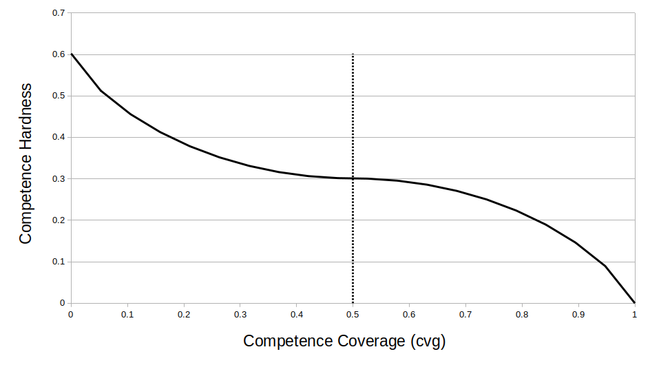
The degree of hardness of a program is determined by the available set of students’ difficulty for covering the program’s competencies. We remind the reader that each required competence is accompanied by an importance weight (Sec 2.1). Thus, consider a program where its most important competence $c_{important}$ (i.e., the competence with the highest $w_{p}(c)$) is very difficult to be covered $h(c_{important},S)\simeq 4\cdot H(0.5)$, then this program is extremely hard. On the other hand, if a specific competence $c$ is somewhat difficult to be covered ($h(c_{important},S)\to 4\cdot H(0.5)$), but it is not very important ($w_{p}(c)\to 0$), then the program is not that hard.

Definition (Program Hardness).

Given a set of students, the hardness of a program $p$ is defined as the aggregation of the hardness for the competences in the program weighted by the importance of each competence: $h(p,S)=W\cdot\sum_{c\in C_{p}}\frac{1}{h(c,S)+\epsilon}\cdot{w_{p}(c)}$, where $W=\frac{1}{\sum_{c\in C_{p}}w_{p}(c)}$ is a normalization factor, and $\epsilon$ is a small positive constant.

In words, the more important and the more difficult a competence is to be covered, the more difficult is to find students with high competence proximity for the program, consequently the harder the program is considered to be. Note that both $w_{p}(c)$ and $h(c)$ are non-negative, so the hardness of one competence cannot be counteracted by the non-hardness of another within the same program.

input : Students $S$, programs $P$, (optionally) sorting order $order$ for $P$

output : team assignment function $g$

1 $V_{p}\leftarrow\bigcup_{p\in P}C_{p}$;

2 for $c\in V_{p}$ do $\mathrm{hc}[c]\leftarrow h(c,S)$;

3 for $p\in P$ do $\mathrm{hp}[p]\leftarrow h(p,S)$;

4 sort $P$ in descending order wrt $\mathrm{hp}$;

5 while $P\neq\emptyset$ do

6       $p\leftarrow$ pop first from $P$;

7       if $|S|\geq m_{p}$ and $\mathrm{hp}[p]<1$ :

8             sort $S$ maximizing coverage in benches of $|C_{p}|$;

             /* assign team to program */

9             $g(p)\leftarrow m_{p}$ fist students in $S$;

10             $S\leftarrow S\setminus g(p)$;

11             update values in $\mathrm{hc}$;

12             if $|S|<1$ : break;

13            

14      

15      

16

17return $g$;

Algorithm 1 Initial Team Allocation

4.2. Improving team allocation

In the second stage we perform a number of random ‘movements’, until convergence to a local or global maximum. The second stage starts with the team assignment produced in the first stage. Thereafter, we iteratively improve the current team assignment either (i) by employing crossovers of students between two programs, and/or (ii) by swapping assigned students with available ones if they exist. Specifically, following Algorithm 2 within an iteration we randomly pick two programs (line 2) and attempt to improve the competence proximity of the pair by exhaustively searching of all possible crossovers of the students assigned to these programs (line 2). However, in order not to computationally overload our algorithm with repetitive exhaustive searches, we perform it only if the following two conditions hold:

1. the two programs share similar competencies; and

2. sine student in one of the teams improves the coverage of some competence of the other team.

In order to evaluate if two programs share similar competencies we exploit the Hausdorff distance Conci and Kubrusly (2018). The Hausdorff distance between the required competencies of two programs $p_{k}$ and $p_{l}$ is defined as:

$$\mathrm{dist}(C_{p_{1}},C_{p_{2}})=\max\big{\{}\min_{c\in C_{p_{1}}}\{\mathrm{cvg}(c,C_{p_{2}})\},\min_{c\in C_{p_{2}}}\{\mathrm{cvg}(c,C_{p_{1}})\}\big{\}}.$$

The above two conditions encode the potentiality of finding an improvement for these two programs, and whether it is worth performimg an exhaustive search. In the exhaustive search, given the students $g(p_{k})\cup g(p_{l})$ we produce all possible partitions that contain two teams of sizes $m_{p_{k}}$ and $m_{p_{l}}$. For each of these partitions we compute the competence proximity of the pair of programs, and yield with the optimum one, i.e., with the partition that achieves the greater competence proximity.

In case we did not achieved any improvements from the previous step and there are available students, i.e. student that have not been assigned to any program, we attempt to swap assigned students with available ones (line  2). That is, we randomly pick a student from either of the two programs, and try to randomly swap them with a student in $S_{available}$. If we achieve an improvement we keep this alteration, otherwise we repeat this process for a fixed number of attempts. In case we succeeded to imporove the competence proximity of the pair, we update the team assignement $g$, the set of availble students $S_{available}$, and the current overall competence proximity (lines 2-2).

In order to overcome the possibility of a series of unsuccessful attempts between random programs, we force a more ‘systematic’ search, which we call local search, on the programs. This local search is performed after a constant number of iterations (line 2). In the local search (line 2) we go through all programs in $P$, swap all members, and check whether some swap improves the overall competence proximity–in the swaps we consider all students: both assigned and available.

Note that Algorithm 2 is anytime algorithm that can yield a result after any number of iterations indicated by the user. However, in its generality, we adopt a notion of convergence in order to terminate the algorithm. That is, we terminate the algorithm (line 2):

• after a number of iterations without no improvements; or

• if we reach an overall competence proximity close to $1$.

Note that we added the latter termination condition in order to avoid unnecessary iterations until convergence, due to the fact that the maximum value the overall competence proximity can reach is $1$. We remind the reader that the competence proximity is the Nash product of the individual competence proximity of the teams to their assigned program (Eq 8), and each individual competence proximity lies in $[0,1]$ (Def 2.2). However, we should make clear that the overall competence proximity does not always reach $1$, but that it can never exceed $1$.

input : Students $S$, programs $P$, team assignment $g$

output : improved team assignment $g$

1 $S_{\mathrm{available}}=S\setminus\bigcup_{p\in P}g(p)$;

2 $\mathrm{current\_cp}=\prod_{p\in P}\mathrm{cp}\big{(}g(p),p\big{)}$;

3 while non_improved and $1-\mathrm{current\_cp}>\varepsilon$ do

4       $p_{k},p_{l}\leftarrow$ randomly select two programs from P;

5      

6      $\mathrm{pair\_cp}=\mathrm{cp}\big{(}g(p_{k}),p_{k}\big{)}\cdot\mathrm{cp}\big{(}g(p_{l}),p_{l}\big{)}$ ;

7       if potentiality($p_{1},p_{2},g$) :

8             $\mathrm{new\_cp},K_{k},K_{l}\leftarrow$ exhaustiveSearch($p_{1},p_{2},g$);

9            

10      

11      else :

12             $\mathrm{new\_cp},K_{k},K_{l}\leftarrow$ localSwaps($p_{1},p_{2},g,S_{\mathrm{available}}$);

13            

14      

15       if $\mathrm{new\_cp}>\mathrm{pair\_cp}$ :

16             $g(p_{k})\leftarrow K_{k}$;

17             $g(p_{l})\leftarrow K_{l}$;

18             $S_{\mathrm{available}}\leftarrow S\setminus\bigcup_{p\in P}g(p)$;

19             $\mathrm{current\_cp}\leftarrow\mathrm{current\_cp}\cdot\frac{\mathrm{new\_cp}}{\mathrm{pair\_cp}}$;

20             $\mathrm{pair\_cp}\leftarrow\mathrm{new\_cp}$;

21            

22      

23       if time for local search :

24             $g,S_{\mathrm{available}},\mathrm{current\_cp}\leftarrow$ localSearch($P,g,S_{\mathrm{available}}$);

25            

26      

27      

28

29 return $g$;

Algorithm 2 Improve Team Allocation

5. Empirical analysis

The purpose of this section is to empirically evaluate the TAIP algorithm along four directions:

• the quality of the solutions that it produces in terms of optimality;

• the quality of the solutions produced by the initial stage;

• the time required by TAIP to produce optimal solutions with respect to CPLEX, an off-the-shelf linear programming solver; and

• the time required by TAIP to yield optimal solutions as the number of students and programs grow.

Overall, our results indicate that TAIP significantly outperforms CPLEX, and hence it is the algorithm of choice to solve the Team Allocation for Internship Programs Problem introduced in this paper. Next, in Sec 5.1 we describe the settings employed in our experiments, whereas Sec 5.2 dissects our results.

5.1. Empirical settings

For our experimental evaluation we used an existing competence ontology provided by Fondazione Bruno Kessler (https://www.fbk.eu/en/); and generated synthetic data in the following way:

Internship program generation

For each program $p$

1. select the required team size $m_{p}\sim\mathcal{U}\{1,3\}$

2. select the number of required competences $|C_{p}|\sim\mathcal{U}\{2,5\}$

3. randomly choose $|C_{p}|$ competences from the ontology

4. the required level function is set to $l_{p}(c)=1,\ \forall\ c\in C_{p}$

5. the weight function is $w_{p}(c)=\mathcal{N}\big{(}\mu=\mathcal{U}(0,1),\sigma=\mathcal{U}(0.01,0.1)\big{)}$ bounded in $(0,1]$ for all $c\in C_{p}$.

Student generation

For each program $p$

1. generate $m_{p}$ new students such that for each student $s$: there are competences $c\in C_{p}$ and $c^{\prime}\in C_{s}$ such that $c^{\prime}$ is (i) identical to $c$; or (ii) a child-node of $c$ in the ontology; uniformly selected among the options.

With these generators we constructed 60 different TAIPP instances, which are shown in Table 2. We solve each problem instance with both TAIP and the IBM CPlex linear programming (LP) solver. The experiments were performed on a PC with Intel Core i7 (8th Gen) CPU, 8 cores, and 8Gib RAM. Moreover, we employed IBM ILOG CPLEX V12.10.0. For all implementations we used Python3.7.

5.2. Results

Quality analysis. Using the optimal solutions yielded by CPLEX as an anchor, we can evaluate the quality of the solutions computed by the TAIP algorithm. Notice that for all problem instances, TAIP reaches the optimal solution. More precisely, for every problem instance, TAIP achieved a solution whose value, in terms of competence proximity, is the same as the value of the optimal solution computed by CPLEX. Fig 2 shows the average quality ratio of TAIPP with respect to CPLEX along time for the problem instances in Table 2. We calculate the quality ratio by dividing the competence proximity computed by TAIP by the optimal value computed by CPLEX, and it is depicted as a percentage (%).

Figure 2. Solution quality achieved by TAIP along time.

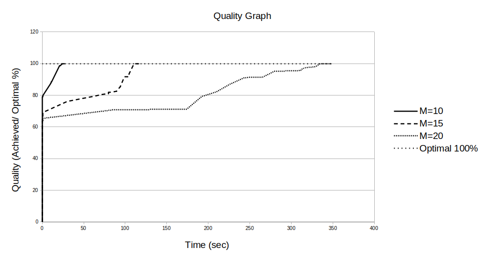
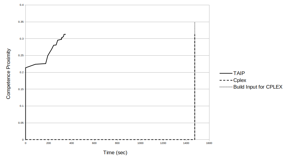
Runtime analysis. The greatest advantage of TAIP is that it is way much faster than CPLEX. As shown in Fig 3 TAIP reaches optimality in less than half of the time required by CPLEX. Specifically, for problem instances with 10 programs, TAIP requires on average $\sim 40\%$ of the time CPLEX needs, i.e., is $\sim 60\%$ faster. As to problem instances with 15 programs, TAIP requires on average $\sim 45\%$ of the time employed by CPLEX ($\sim 55\%$ faster). Finally, for problem instances with 20 programs, TAIP requires on average $\sim 29\%$ of the time spent by CPLEX ($\sim 71\%$ faster). Therefore, the larger the size of the problem instances, the larger the benefits for TAIP with respect to CPLEX. Here we should note that the time consuming task for CPLEX is the building of the LP encoding the problem, while solving the actual problem is done in seconds. This indicates that the problem instances under investigation are rather large than hard: as the number of programs increases, so does the number of students, resulting in large linear programs.

(a) 10 programs

(b) 15 programs

(c) 20 programs

Figure 3. Average Competence Proximity vs Time

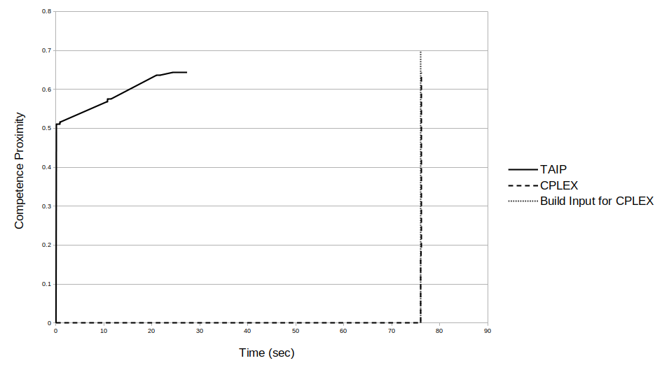
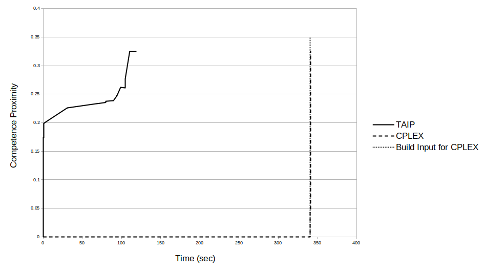
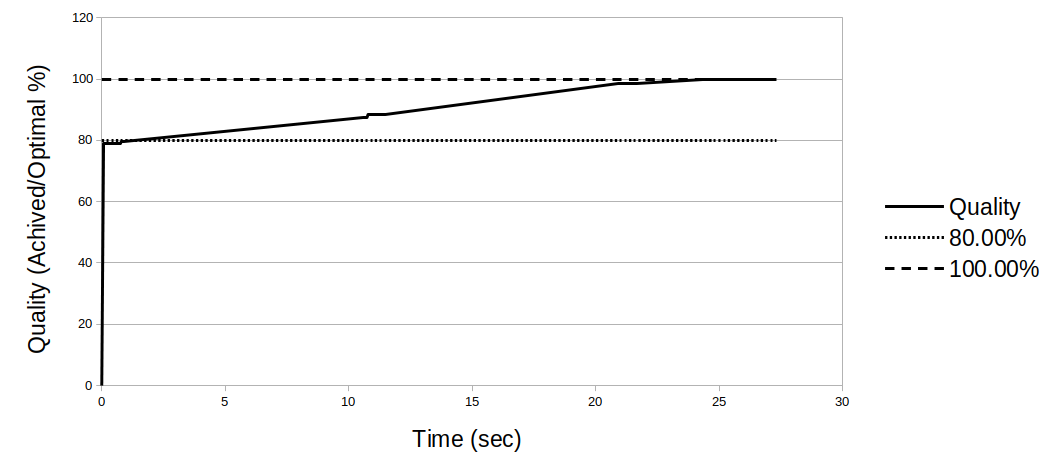
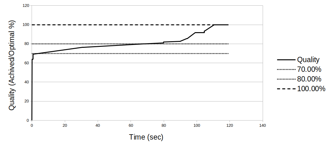
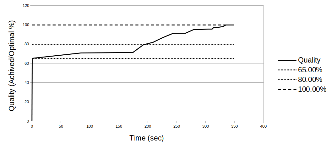
Anytime analysis. Last but not least we present our results on the anytime behavior of TAIP, as shown in Fig 4. We observe that after completing the initial stage described in Sec 4.1, the solution quality produced by TAIP reaches 80%, 70%, and 65% of the optimal solution, for problem instances with 10,15 and 20 programs respectively. Furthermore, TAIP reaches quality 80% in $0.001\times t_{CPLEX}$ for 10 programs, 70% in $0.025\times t_{CPLEX}$ for 15 programs, and 65% in $0.0002\times t_{CPLEX}$ for 20 programs, where $t_{CPLEX}$ is the time CPLEX needs to compute the optimal solution. Moreover, in all investigated settings we reached 80% quality in less than 20% of the time CPLEX needs: 0.1%, 20%, and 13.5% of CPLEX time for 10,15, and 20 programs.

(a) 10 programs

(b) 15 programs

(c) 20 programs

Figure 4. Anytime Behavior

6. Conclusions and future work

Here we formally defined the problem of Team Allocation for Internship Programs Problem. We first studied the problem’s complexity and characterised its search space.Thereafter, we provided an encoding to otimally solve the TAIPP by means of linear programming. Then, we proposed a novel, heuristic anytime algorithm, TAIP. Finally, we conducted a systematic comparison of TAIP versus the CPLEX LP solver when solving TAIPP problem instances. Our experimental evaluation showed that TAIP outperforms CPLEX in time, mainly because of the extremely large input that the latter requires. Moreover, TAIP always managed to reach the optimal solution for the problem instances under investigation. Specifically TAIP converged to the optimal in less than 40% of the time required by CPLEX, and achieved a quality of 80% in less than 20% of the time required by CPLEX. As future work, we itend to device more intelligent strategies during the second state of TAIPP, instead of our current randomized strategy. Furthermore, in the future we will study the performance of TAIP on actual-world data.

Dataset	1	2	3	4	5	6	7	8	9	10	11	12	13	14	15	16	17	18	19	20	Average
N=#Students	18	20	21	19	22	19	24	18	19	20	23	20	18	19	25	21	25	20	17	13	20.5

(a) Family of datasets with 10 programs

Dataset	21	22	23	24	25	26	27	28	29	30	31	32	33	34	35	36	37	38	39	40	Average
N=#Students	23	33	32	29	33	40	31	32	28	25	27	31	29	28	32	29	29	32	34	29	30.6

(b) Family of datasets with 15 programs

Dataset	41	42	43	44	45	46	47	48	49	50	51	52	53	54	55	56	57	58	59	60	Average
N=#Students	44	45	44	45	38	42	42	47	41	44	37	36	42	37	47	32	40	37	44	43	41.35

(c) Family of datasets with 20 programs

Table 2. Synthetic problem instances.

References

- (1)
- Al-sharhan et al. (2001) S. Al-sharhan, F. Karray, W. Gueaieb, and O. Basir. 2001. Fuzzy entropy: a brief survey. In 10th IEEE International Conference on Fuzzy Systems. (Cat. No.01CH37297), Vol. 3. 1135–1139 vol.2. https://doi.org/10.1109/FUZZ.2001.1008855
- Anagnostopoulos et al. (2012) Aris Anagnostopoulos, Luca Becchetti, Carlos Castillo, Aristides Gionis, and Stefano Leonardi. 2012. Online Team Formation in Social Networks. WWW’12 - Proceedings of the 21st Annual Conference on World Wide Web, 839–848. https://doi.org/10.1145/2187836.2187950
- Andrejczuk (2018) Ewa Andrejczuk. 2018. Artificial intelligence methods to support people management in organisations. Doctoral.
- Andrejczuk et al. (2018) Ewa Andrejczuk, Rita Berger, Juan A. Rodríguez-Aguilar, Carles Sierra, and Víctor Marín-Puchades. 2018. The composition and formation of effective teams: computer science meets organizational psychology. Knowledge Eng. Review 33 (2018), e17. https://doi.org/10.1017/S026988891800019X
- Andrejczuk et al. (2019) Ewa Andrejczuk, Filippo Bistaffa, Christian Blum, Juan A. Rodríguez-Aguilar, and Carles Sierra. 2019. Synergistic team composition: A computational approach to foster diversity in teams. Knowledge-Based Systems 182, 104799 (10/2019 2019). https://doi.org/10.1016/j.knosys.2019.06.007
- Conci and Kubrusly (2018) AURA Conci and CS Kubrusly. 2018. Distance Between Sets-A survey. arXiv preprint arXiv:1808.02574 (2018).
- Crawford et al. (2016) Chad Crawford, Zenefa Rahaman, and Sandip Sen. 2016. Evaluating the Efficiency of Robust Team Formation Algorithms. In Autonomous Agents and Multiagent Systems, Nardine Osman and Carles Sierra (Eds.). Springer International Publishing, Cham, 14–29.
- Kargar et al. (2012) Mehdi Kargar, Aijun An, and Morteza Zihayat. 2012. Efficient Bi-objective Team Formation in Social Networks. In Machine Learning and Knowledge Discovery in Databases, Peter A. Flach, Tijl De Bie, and Nello Cristianini (Eds.). Springer Berlin Heidelberg, Berlin, Heidelberg, 483–498.
- Li et al. (2003) Y. Li, Z. A. Bandar, and D. Mclean. 2003. An approach for measuring semantic similarity between words using multiple information sources. IEEE Transactions on Knowledge and Data Engineering 15, 4 (July 2003), 871–882. https://doi.org/10.1109/TKDE.2003.1209005
- Luca and Termini (1974) Aldo De Luca and Settimo Termini. 1974. Entropy of L-fuzzy sets. Information and Control 24, 1 (1974), 55 – 73. https://doi.org/10.1016/S0019-9958(74)80023-9
- Maddox (2002) R. B. Maddox. 2002. Mathematical Thinking and Writing: A transition to abstract mathematics (1st ed.). Academic Pr, San Diego.
- Osman et al. (2014) N. Osman, C. Sierra, F. Mcneill, J. Pane, and J. Debenham. 2014. Trust and Matching Algorithms for Selecting Suitable Agents. ACM Trans. Intell. Syst. Technol. 5, 1, Article 16 (Jan. 2014), 39 pages. https://doi.org/10.1145/2542182.2542198
- Sandholm et al. (2002) Tuomas Sandholm, Subhash Suri, Andrew Gilpin, and David Levine. 2002. Winner Determination in Combinatorial Auction Generalizations. In Proceedings of the First International Joint Conference on Autonomous Agents and Multiagent Systems: Part 1 (AAMAS ’02). Association for Computing Machinery, New York, NY, USA, 69–76. https://doi.org/10.1145/544741.544760
- Zadeh (1965) L.A. Zadeh. 1965. Fuzzy sets. Information and Control 8, 3 (1965), 338 – 353. https://doi.org/10.1016/S0019-9958(65)90241-X