$\mathrm{C}^{18}\mathrm{O}$, ${}^{13}\mathrm{CO}$, and ${}^{12}\mathrm{CO}$ abundances
and excitation temperatures in the Orion B molecular cloud

Abstract

Context. CO isotopologue transitions are routinely observed in molecular clouds to probe the column density of the gas, the elemental ratios of carbon and oxygen, and to trace the kinematics of the environment.

Aims. We aim at estimating the abundances, excitation temperatures, velocity field and velocity dispersions of the three main CO isotopologues towards a subset of the Orion B molecular cloud, which includes IC 434, NGC 2023, and the Horsehead pillar.

Methods. We use the Cramer Rao Bound (CRB) technique to analyze and estimate the precision of the physical parameters in the framework of local-thermodynamic-equilibrium (LTE) excitation and radiative transfer with an additive white Gaussian noise. We propose a maximum likelihood estimator to infer the physical conditions from the 1$-$0 and 2$-$1 transitions of CO isotopologues. Simulations show that this estimator is unbiased and efficient for a common range of excitation temperatures and column densities ($T_{\mathrm{ex}}>6\mathrm{\,K}$, $N>10^{14}\,-\,10^{15}\leavevmode\nobreak\ \mathrm{\,cm^{-2}}$).

Results. Contrary to the general assumptions, the different CO isotopologues have distinct excitation temperatures, and the line intensity ratios between different isotopologues do not accurately reflect the column density ratios. We find mean fractional abundances that are consistent with previous determinations towards other molecular clouds. However, significant local deviations are inferred, not only in regions exposed to UV radiation field but also in shielded regions. These deviations result from the competition between selective photodissociation, chemical fractionation, and depletion on grain surfaces. We observe that the velocity dispersion of the C¹⁸O emission is 10% smaller than that of ¹³CO. The substantial gain resulting from the simultaneous analysis of two different rotational transitions of the same species is rigorously quantified.

Conclusions. The CRB technique is a promising avenue for analyzing the estimation of physical parameters from the fit of spectral lines. Future work will generalize its application to non-LTE excitation and radiative transfer methods.

1 Introduction

Spectroscopic measurements are commonly used to probe astrophysical objects. In the interstellar medium, the moderate temperatures and densities of diffuse and molecular clouds ($T_{\mathrm{kin}}\sim 10-100\mathrm{\,K}$, and $n\sim 10^{2}-10^{5}\mathrm{cm}^{-3}$, Draine 2011) are well suited for the emission in the low energy rotational lines of molecules such as carbon monoxide, which are accessible at millimeter wavelengths. The advent of sensitive broadband heterodyne receivers provides homogeneous data sets of various CO isotopologues and other species with high signal-to-noise ratios over large fields of view. The ORION-B IRAM-30m large program (Outstanding Radio-Imaging of OrioN B, co-PIs: J. Pety and M. Gerin) aims at imaging 5 square degrees towards the southern part of the Orion B molecular cloud over most of the 3 mm atmospheric window. Carbon monoxide is especially interesting because it is one of the most abundant molecules after molecular hydrogen. Using the unsupervised meanshift clustering method on the intensities of the CO isotopologues, Bron et al. (2018) show that it is possible to cluster the emission line data across the analyzed field of view into a few classes of increasing (column) densities. In two empirical studies, Gratier et al. (2017) and Gratier et al. (submitted as a companion paper) show qualitatively and quantitatively that the ${}^{12}\mathrm{CO}$(1$-$0), ${}^{13}\mathrm{CO}$(1$-$0), and $\mathrm{C}^{18}\mathrm{O}$(1$-$0) lines are indeed tracing the molecular gas well. Their quantitative comparisons show that the $\mathrm{H_{2}}$ column density deduced from the dust emission can be accurately estimated from the ${}^{12}\mathrm{CO}$(1$-$0), ${}^{13}\mathrm{CO}$(1$-$0), and $\mathrm{C}^{18}\mathrm{O}$(1$-$0) lines in the column density range from $10^{21}$ to $\gtrsim 10^{22}\mathrm{\,cm^{-2}}$.

Assuming identical excitation temperatures, the opacity of the ground state transitions is expected to be smaller for ${}^{13}\mathrm{CO}$ than for ${}^{12}\mathrm{CO}$, and even smaller for $\mathrm{C}^{18}\mathrm{O}$ because of the difference in elemental abundances, $\mathrm{{}^{12}C/^{13}C\sim 60}$ and $\mathrm{{}^{16}O/^{18}O\sim 500}$ (Langer & Penzias, 1990; Wilson & Rood, 1994). These three lines can thus be used to probe progressively higher gas column densities, provided the relative elemental abundances are constant and the CO isotopologue abundances track the elemental abundances. However chemical models and observations show that selective photodissociation and carbon isotopic fractionation can significantly modify the relative abundances of carbon monoxide isotopologues, as compared to elemental abundances (Visser et al., 2009; Liszt, 2017; Roueff et al., 2015). Fractionation via the exchange reaction between ¹³C⁺ and ¹²CO leads to an enhancement of the ¹³CO abundance in the diffuse/translucent regions where CO and C⁺ coexist and the kinetic temperature remains moderate ($\lesssim 50\mathrm{\,K}$, Liszt & Pety 2012). This mechanism widens the ${}^{13}\mathrm{CO}$ emitting region and brings it closer to that of ${}^{12}\mathrm{CO}$, which favors the simultaneous detection of both isotopologues on wide fields of view. However the ratio of isotopologue abundances can be significantly different from the ratio of elemental abundances, which complicates the determination of the $\mathrm{{}^{13}C}$ elemental abundance from CO observations only. Up to now, the most reliable determinations of the $\mathrm{{}^{12}C/^{13}C}$ elemental abundance ratio have been obtained using $\mathrm{C^{+}}$ or C observations in regions without significant fractionation (e.g. Keene et al., 1998; Ossenkopf et al., 2013), or involve $\mathrm{C}^{18}\mathrm{O}$ and the doubly isotopic species ¹³C¹⁸O (Langer & Penzias, 1990).

No such fractionation reaction exists for oxygen. However, the more abundant CO isotopologues shield themselves from the destructive effect of UV photons more efficiently than less abundant isotopologues because the photodissociation of carbon monoxide is governed by line absorption. This effect called selective photodissociation is important. It has been studied in detail through laboratory experiments (e.g. Stark et al., 2014) and in models of photo-dissociation regions (e.g. Visser et al., 2009). In observations, it is clearly seen as an offset between the threshold for the apparition of ${}^{12}\mathrm{CO}$ (near $A_{\mathrm{V}}=0.5\,\mathrm{mag}$) and $\mathrm{C}^{18}\mathrm{O}$ $(1.5\,\mathrm{mag})$ in the Taurus molecular cloud, and this offset is not due to a difference in the detection sensitivity (Frerking et al., 1989; Cernicharo & Guelin, 1987). Typically, the ¹³CO abundance is enhanced through fractionation in the same regions where the C¹⁸O abundance decreases due to selective photodissociation. This leads to a broad range of the ¹³CO/C¹⁸O abundance ratio for a given set of elemental abundances.

Determining the ratio of elemental abundances of the C and O isotopes is interesting because it provides information on the stellar populations which have produced these elements. Some external galaxies exhibit CO isotopologue ratios that significantly differ from the expected value based on the mean elemental abundances in the solar neighborhood. Such differences can trace differences in elemental abundances, hence in stellar populations and IMF shape (Sliwa et al., 2017; Martín et al., 2019). However, a proper account of isotopic chemistry described above must be performed in order to use the information on the relative abundances of the CO isotopologues.

Finally, Orkisz et al. (2019) show, in an analysis of the filamentary structure of the Orion B molecular cloud, that the gas velocity dispersion determined from $\mathrm{C}^{18}\mathrm{O}$ reaches a minimum value in the filament ridges, that it is always lower than the velocity dispersion determined by ${}^{13}\mathrm{CO}$. This suggests that this variation of velocity dispersion between CO isotopologue traces the dissipation of turbulence when entering the dense filaments inside molecular clouds.

Constraining all these astrophysical effects relies on a precise derivation of physical conditions and chemical composition from spectroscopic observations. This in turn relies on the resolution of the radiative transfer equation because the line intensities and profiles bear information on the line emission mechanisms. The large data volumes provided by observational programs like ORION-B require new statistical analysis methods using the information in an optimal way, and a derivation of the physical parameters and their associated errors with a rigorous methodology. For instance, the emission of the lowest rotational transitions of the three major isotopologues of carbon monoxide, ¹²CO, ¹³CO, and C¹⁸O is commonly used to determine the molecular gas column density and evaluate the mass of molecular gas. Because these lines can now be observed simultaneously, leading to an homogeneous flux calibration and therefore precise relative calibration, it is essential to have a good estimation of the precision on the mass estimate.

In estimation theory, the Cramer Rao bound (CRB) provides a precision of reference that does not depend on a specific estimator of the searched quantity, but only on the physical model and the statistical properties of the noise (see, e.g., Bonaca & Hogg, 2018; Espinosa et al., 2018). The CRB further allows the quantification of the loss of precision due to degeneracies between the estimated parameters (for instance column density and excitation temperature). Hence, a large value of this bound indicates insufficient data or knowledge with respect to a given physical model. We will here apply this technique in the simplest possible model framework, i.e., the emission of lines in Local Thermodynamic Equilibrium (LTE), which can be fully expressed with analytical equations.

The level populations of interstellar molecules result from the balance of collisional (and possibly radiative) excitation and radiative & collisional de-excitation. Therefore the level populations often deviate from LTE conditions because the collisions are not efficient enough to populate all energy levels according to a Boltzmann distribution. With its low dipole moment (0.1 Debye) and high abundance relative to H₂, the low energy rotational lines of carbon monoxide are bright and easily thermalized in collisions with H₂, H and He. This means that the LTE model is still a good approximation for this molecule, i.e., the rotational level populations can be described by a Boltzman distribution at a single excitation temperature (Liszt, 2006; Leung & Liszt, 1976; Goldsmith & Langer, 1999; Goldreich & Kwan, 1974). Deviations from the LTE model have been theoretically studied. For instance, using non local, non LTE radiative transfer models of a uniform (constant density and temperature) spherical cloud, Bernes (1979) shows that the excitation temperatures of the ${}^{12}\mathrm{CO}$(1$-$0) and ${}^{12}\mathrm{CO}$(2$-$1) lines exhibit moderate spatial variations from edge to center. It is concluded that the LTE model is mostly valid for the ground state transition and deviations from this approximation increase with the quantum number of the upper level (van der Tak et al., 2007).

With a wide range of physical conditions, from bright far-UV illuminated regions to cold and shielded regions through diffuse and translucent gas irradiated by a moderate radiation field, the Orion B molecular cloud is an ideal place to probe to which extent fractionation and selective photodissociation can modify the elemental abundance ratio. It is also a good region to probe the differences in excitation between isotopologues as the simple hypothesis of equal excitation temperatures for ${}^{12}\mathrm{CO}$, ${}^{13}\mathrm{CO}$ and $\mathrm{C}^{18}\mathrm{O}$ may not be valid, as discussed in Bron et al. (2018).

The article is organized as follows. Section 2 presents the data used in this paper. Section 3 summarizes the mathematical formulation of the LTE radiative transfer. Section 4 computes and analyzes the precision achievable for this theoretical framework. Section 5 illustrates the proposed methodology on actual data sets. Section 6 focuses on the astrophysical interpretations of these results. Appendix A details the calculation of some gradients necessary to compute the Fisher matrix. Appendix B describes our implementation of the maximum likelihood estimator, and appendix C discusses the performance of this estimator.

Figure 1: Spatial distributions of the integrated intensity (in $\mathrm{\,K\,km\,s^{-1}}$) of the considered lines. The maps have been rotated counterclockwise by 14 degrees from the RA/DEC J2000 reference frame. The spatial offsets are given in arcsecond from the projection center located at $\mathrm{05^{h}40^{m}54.270^{s},-02^{\circ}28^{{}^{\prime}}00.00^{{}^{\prime\prime}}}$. Red crosses stand for two particular lines of sight which are analyzed in Figure 10.

Table 1: Properties of observed lines.

Species	Line	$\nu$	$dV$	Beam	Noise
		MHz	$\mathrm{\,km\,s^{-1}}$	′′	mK
C18O	1$-$0	109782.173	0.5	23.5	116
C18O	2$-$1	219560.319	0.5	23.5	96
13CO	1$-$0	110201.354	0.5	23.5	116
13CO	2$-$1	220398.686	0.5	23.5	134
12CO	1$-$0	115271.202	0.5	23.5	278

2 Description of the data

We will try to estimate the velocity field, the column density, and the excitation temperature of the CO isotopologues from the analysis of the ${}^{13}\mathrm{CO}$(1$-$0), ${}^{13}\mathrm{CO}$(2$-$1), $\mathrm{C}^{18}\mathrm{O}$(1$-$0), $\mathrm{C}^{18}\mathrm{O}$(2$-$1) and ${}^{12}\mathrm{CO}$(1$-$0) lines towards parts of the Orion B molecular cloud. We will compare our results with the dust-traced H₂ column density and dust temperature. This section describes the associated data sets.

2.1 IRAM-30m observations

2.1.1 3 mm CO lines from the ORION-B large program

The 3 mm data were obtained with the IRAM-30m as part of the ORION-B large program. Pety et al. (2017) present in detail the acquisition and reduction of the dataset used in this study. In short, the used data were acquired at the IRAM-30m telescope using the EMIR receiver and Fourier transform spectrometer from August 2013 to November 2014. The frequency range from 84 to 116 GHz was completely sampled at 200 kHz spectral resolution. The $J=1-0$ lines of the CO isotopologues analyzed here are observed in a single receiver tuning. These lines are thus well inter-calibrated. The absolute flux calibration at 3 mm for the IRAM-30m telescope is estimated to be better than 5%.

2.1.2 1 mm CO lines

The ${}^{13}\mathrm{CO}$(2$-$1) and $\mathrm{C}^{18}\mathrm{O}$(2$-$1) were also observed at the IRAM-30m in 2006 (PI: N. Peretto) using the ABCD generation of receivers and the VESPA auto-correlator. The two lines were observed simultaneously ensuring an excellent inter-calibration.

Data reduction was carried out using the GILDAS/CLASS software. The contribution of the atmosphere was first removed (ON-OFF procedure) and the data were calibrated to the $T_{A}^{\star}$ scale using the standard chopper-wheel method (Penzias & Burrus, 1973). The data were then converted to main-beam temperatures using the standard forward (0.94) and main-beam (0.62) efficiencies for the ABCD receiver around 220 GHz. The resulting absolute flux calibration is estimated to be better than 10%. We subtracted a first order baseline from every spectrum, excluding the velocity range from 5 to 15$\mathrm{\,km\,s^{-1}}$ in the Local Standard of Rest (LST) frame. The spectra were finally gridded into a data cube through a convolution with a Gaussian kernel of full width at half maximum $\sim 1/3$ of the IRAM-30m telescope beamwidth at the line rest frequency.

2.2 Herschel observations

In order to get independent constraints on the physical conditions in the Orion B cloud, we use the dust continuum observations from the Herschel Gould Belt Survey (André et al., 2010; Schneider et al., 2013) and from the Planck satellite (Planck Collaboration I, 2011). The fit of the spectral energy distribution by Lombardi et al. (2014) gives us access to the spatial distributions of the dust opacity at $850\mathrm{\,\mu m}$ and of the dust temperature. As in Pety et al. (2017), we converted $\tau_{850\mathrm{\,\mu m}}$ to visual extinctions using $A_{\mathrm{V}}=2.7\times 10^{4}\,\tau_{850}\,\mathrm{mag}$, and the visual extinction into H₂ column density using $N(\mathrm{H_{2}})/A_{\mathrm{V}}=0.9\times 10^{21}\,\mathrm{H\,cm^{-2}\,mag^{-1}}$.

2.3 Field of view

We will jointly analyze the $J=1-0$ and $J=2-1$ lines of the CO isotopologues. We thus restrict the field of view to the region that was observed at 3 and 1 mm. This covers $19^{\prime}\times 26^{\prime}$ towards the Orion B molecular cloud part that contains the Horsehead nebula, and the Hii regions NGC 2023 and IC 434. The cubes used here are rotated counterclockwise by $14\degr$ around the projection center ($\mathrm{05^{h}40^{m}54.270^{s},-02^{\circ}28^{{}^{\prime}}00.00^{{}^{\prime\prime}}}$) in the RA/DEC J2000 reference frame (see Fig. 1). The coordinates are given in offsets $(\delta x,\delta y)$ in arcseconds from this projection center. The IRAM-30m angular resolution ranges from $11.5^{\prime\prime}$ at 220 GHz to $23.5^{\prime\prime}$ at 110 GHz. The position-position-velocity cubes of each line were smoothed to a common angular resolution of $23.5^{\prime\prime}$ to avoid resolution effects during the comparison. At a distance of 400 pc (Menten et al., 2007), the sampled linear scales range from $\sim 0.045\mathrm{\,pc}$ to $\sim 3\mathrm{\,pc}$.

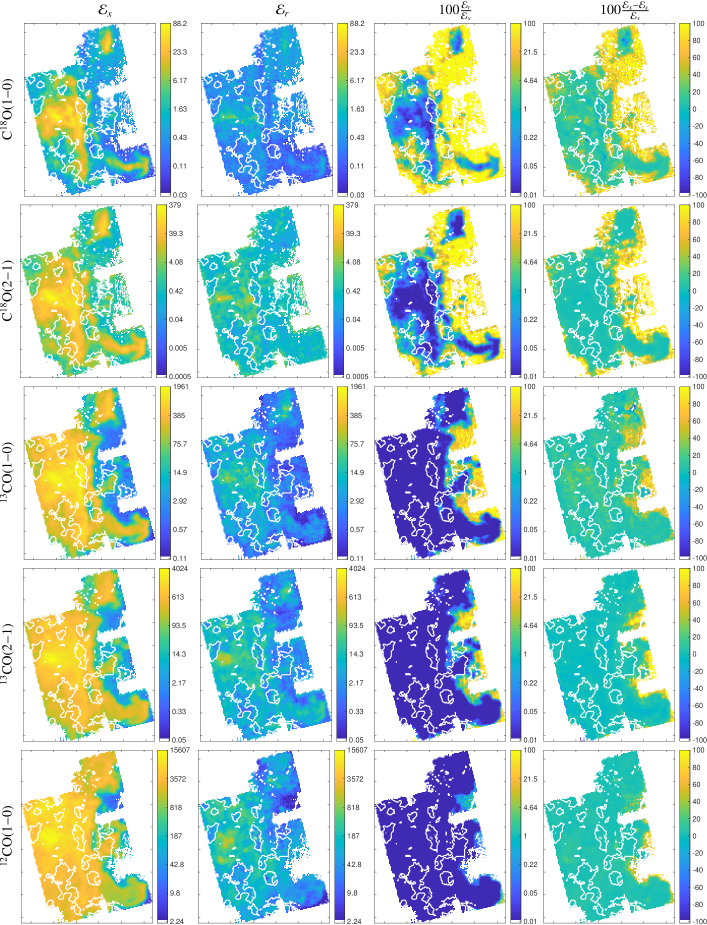
The spectral and spatial axes were resampled in order to share the same spatial grid and velocity axis for all lines. The spectroscopic observations thus provide position-position-velocity cubes of $129\times 170\times 80$ pixels, each pixel covering $9^{\prime\prime}\times 9^{\prime\prime}\times 0.5\mathrm{\,km\,s^{-1}}$ (Nyquist sampling at 3 mm). Figure 1 shows the maps of the intensity integrated between 0 and $20\mathrm{\,km\,s^{-1}}$ for the five lines of interest.

2.4 Noise

In this paper, the standard deviation of the noise $\sigma_{b}$ is estimated only on negative values of each spectrum through

$$\sigma_{b}=\left(\frac{1}{K_{\mathrm{neg}}}\sum_{k\in\{T_{k}\leq 0\}}T_{k}^{2}\right)^{1/2},$$ (1)

where $T$ is the intensity in Kelvin, and $K_{\mathrm{neg}}$ the number of channels that have a negative value of the intensity. This allows us to compute it without a priori information on the velocity range where the line appears, but it assumes that the baselining removed any intensity offset. Table 1 lists the median noise estimated after spectral resampling and angular smoothing.

2.5 Line profiles

A fraction of the studied field of view shows spectra that can only be modeled with more than one velocity component along the line of sight. While we will adapt our formalism to handle such cases, it is not obvious to devise a robust statistical test to deduce the best number of components that must be used. This is particularly true at transitions between regions where the number of required velocity components changes to get a good fit. To address this issue, we used the ROHSA (Marchal et al., 2019) algorithm that makes a Gaussian decomposition based on a multi-resolution process from coarse to fine grid. We only used here the spectra denoised by ROHSA to provide a spatially coherent estimation of the number of components and some initial estimation of their associated central velocities for each pixel.

3 Radiative Transfer in Local Thermodynamic Equilibrium

Molecular line emission and absorption in the case of Local Thermodynamic Equilibrium (LTE) are well known (see, e.g., Mangum & Shirley, 2015). In this Section, we just summarize the associated notations and equations so that we can easily explain the precision analysis framework on this case in the next section. For the sake of simplicity, we focus on a single chemical species and a single velocity component along one line of sight. The observed spectrum as a function of frequency $\nu$ is defined as

$$x(\nu)=s(\nu)+b(\nu),$$ (2)

where $b$ is a (thermal) Gaussian noise, and $s$ is the spectrum associated to the species of interest. The specific intensity $s$ and the associated measurement noise $b$ are expressed in Kelvins following the standard use in radioastronomy. The data reduction (atmospheric ON-OFF calibration and spectrum baselining to subtract the slowly-varying continuum residual from the receiver and the atmosphere) delivers a noise $b$ that is centered (i.e., with zero-mean), and whose variance can be considered constant over each line profile.

We assume that two lines $(l\in\{1,2\})$ from the same species are observed. The photons of each line are emitted at the rest frequency of the line, $\nu_{l}$, and redshifted in frequency because of the Doppler shift due to the motion of the gas along the line of sight in the observation frame, typically the Local Standard of Rest (LSR). The photon is thus received at the redshifted frequency $\nu^{\mathrm{red}}_{l}=\nu_{l}\left(1-\frac{V}{c}\right)$, where $V$ is the velocity of the emitting cell of gas in the LSR frame and $c$ is the speed of light. This equation is the radio low-velocity approximation of the Doppler effect. The Doppler effect due to the motion of the observer relative to the LSR is automatically taken into account in the data acquisition process. Therefore, each line of the dataset is analyzed in the LSR frame. In this frame each line is centered around a typical velocity, noted $\Delta_{V}$. This velocity is related to the redshifted centroid frequency of the line, $\nu^{\mathrm{cent}}_{l}$, through a particular case of the previous equation

$$\nu^{\mathrm{cent}}_{l}=\nu_{l}\left(1-\frac{\Delta_{V}}{c}\right).$$ (3)

We assume that the only background source of emission is the Cosmic Microwave Background (CMB). In this case, the intensity $s$ at observed frequency $\nu$ around $\nu^{\mathrm{red}}_{l}$ can be written as

$$s(\nu)=\left\{J(T_{\mathrm{ex}},\nu_{l})-J(T_{\mathrm{CMB}},\nu)\right\}\left[1-\exp(-\Psi(\nu))\right]$$ (4)

where $T_{\mathrm{CMB}}$ is the known CMB temperature ($T_{\mathrm{CMB}}=2.73\mathrm{\,K}$, Mather et al. 1994), $T_{\mathrm{ex}}$ is the unknown excitation temperature along the line of sight, and $J$ is a measure of intensity at a given temperature

$$J(T,\nu)=\frac{c^{2}}{2k\nu^{2}}B(T,\nu)=\frac{h\nu}{k}\frac{1}{\exp{\frac{h\nu}{kT}}-1},$$ (5)

where $B(T,\nu)$ is the spectral distribution of the radiation of a black body at temperature $T$. The term $\left[1-\exp(-\Psi(\nu))\right]$ in Eq. (4) represents the emission/absorption by the emitting/absorbing medium along the line of sight, considered as a uniform slab. The function $\Psi$ is the profile that corresponds to the integrated opacity through the whole slab. For each line $l$, it can be written as

$$\Psi_{l}(\nu)=\alpha_{l}\,\phi\left(\nu;\nu^{\mathrm{cent}}_{l},\nu_{l}\frac{\sigma_{V}}{c}\right).$$ (6)

In this equation, $\sigma_{V}$ is the velocity dispersion of the source along the line of sight. It varies as a function of the local physical conditions (higher temperatures and higher turbulence will lead to larger values). The function $\phi$ is a Gaussian profile

$$\phi(\nu;\nu_{o},\sigma_{\nu})=\frac{1}{\sqrt{2\pi}\sigma_{\nu}}\exp\left(-\frac{(\nu-\nu_{o})^{2}}{2\sigma_{\nu}^{2}}\right),$$ (7)

where $\sigma_{\nu}$ is the frequency dispersion in the source rest frame. It is related to $\sigma_{V}$ by $\sigma_{\nu}=\nu_{l}\,\sigma_{V}/c$, because of the Doppler effect. Finally, the amplitude $\alpha_{l}$ associated to the Gaussian profile $\phi$ and line $l$ is

$$\alpha_{l}=\frac{c^{2}}{8\pi}\frac{N}{Q(T_{\mathrm{ex}})}\frac{A_{l}\,g_{\mathrm{up}}}{\nu_{l}^{2}}\exp\left[-\frac{E_{\mathrm{up}}}{T_{\mathrm{ex}}}\right]\left(\exp\left[\frac{h\,\nu_{l}}{k\,T_{\mathrm{ex}}}\right]-1\right)$$ (8)

where $A_{l}$ is the Einstein spontaneous emission rate for line $l$, $g_{\mathrm{up}}$ is the degeneracy of the upper level of the line, $E_{\mathrm{up}}$ its energy (in units of Kelvin), and $N$ the column density of the species along the line of sight. The partition function $Q(T_{\mathrm{ex}})$ is tabulated in molecular databases (e.g., CDMS, Müller et al. 2001, or JPL, Pickett et al. 1998), and its temperature dependence can be interpolated for each species. The partition function is computed as the sum of the populations of all energy levels $E_{k}$. If the energy levels are expressed in Kelvin, $Q(T_{\mathrm{ex}})$ can be written as

$$Q(T_{\mathrm{ex}})=\sum_{k=1}^{+\infty}g_{k}\exp\left[-\frac{E_{k}}{T_{\mathrm{ex}}}\right].$$ (9)

The parameter $\alpha_{l}$ is related to the line opacity $\tau_{l}$

$$\tau_{l}=\frac{\alpha_{l}\,c}{\sqrt{2\pi}\nu_{l}\sigma_{V}},$$ (10)

which is dimensionless. The excitation temperature is defined from the ratio of the population in the upper ($n_{\mathrm{up}}$) and lower ($n_{\mathrm{low}}$) levels of the studied line

$$\frac{n_{\mathrm{up}}}{n_{\mathrm{low}}}=\frac{g_{\mathrm{up}}}{g_{\mathrm{low}}}\exp\left[-\frac{h\nu_{l}}{kT_{\mathrm{ex}}}\right].$$ (11)

When the molecules are in thermal equilibrium with their environment, the temperature $T_{\mathrm{ex}}$ is equal to the gas kinetic temperature. The kinetic temperature is not known and must be estimated.

In the previous equations, the physical characteristics of the gas ($N$, $T_{\mathrm{ex}}$, $\sigma_{V}$, and $\Delta_{V}$) depend on the specific line of sight on the sky. Moreover, while observers try to get a uniform noise when observing the source, this is never perfect and it is important to assume that the noise standard deviation $\sigma_{b}$ also depends on the specific line of sight on the sky. These considerations imply that $\alpha_{l}$, $\tau_{l}$, $\nu^{\mathrm{cent}}_{l}$, $\Psi_{l}$, $s$, and $x$ will also depend on the sky position.

4 Cramer-Rao Bound analysis

Figure 2: Variations of the square root of the Cramer-Rao Bound (CRB) of the centroid velocity ($\Delta_{V}$, left panel) and velocity dispersion ($\sigma_{V}$, middle panel) in $\mathrm{\,km\,s^{-1}}$ as a function of the column density and the excitation temperature. The right panel shows the variations of a function of the product of the number of channels $(K)$ and the signal-to-noise ratio $({\cal R})$. In all three cases, data are simulated assuming that ${}^{13}\mathrm{CO}$(1$-$0) and ${}^{13}\mathrm{CO}$(2$-$1) are measured and the unit of the image contours are $\mathrm{\,km\,s^{-1}}$. In this simulation, $\sigma_{b}=100\mathrm{\,mK}$, $\Delta_{V}=1.1\mathrm{\,km\,s^{-1}}$ and $\sigma_{V}=0.61\mathrm{\,km\,s^{-1}}$.

In this article, we aim at estimating the physical parameters of the LTE model presented in section 3 on the ORION-B data (see section 2). Even when the LTE model is perfectly verified, the presence of an additive Gaussian noise induces some uncertainty on the estimation. For each physical parameter $\theta$ estimated as $\widehat{\theta}$, the estimation error $(\widehat{\theta}-\theta)$ can be quantified with the mean square error (MSE) $\langle(\widehat{\theta}-\theta)^{2}\rangle$, where $\langle.\rangle$ represents the statistical mean over the different realizations of the noise $b$. MSE can be estimated with Monte Carlo simulations, but the result then depends on the choice of the implemented estimator. For example, when MSE is large, one does not know whether it is due to the choice of the estimator or to a lack of information in the data. In estimation theory, the Fisher matrix allows to quantify the amount of information in the considered problem. It provides a reference precision, named Cramer-Rao Bound (CRB), which does not depend on the choice of a specific estimator of the searched quantity, but only on the physical model and the statistical properties of the noise (see, e.g., Bonaca & Hogg, 2018; Espinosa et al., 2018).

Mathematically speaking, the CRB noted ${\cal B}(\theta)$ is simply a lower bound on the MSE of unbiased estimators (see Eq. (15)). Indeed, the MSE is equal to the estimation variance $\langle(\widehat{\theta}-\langle\widehat{\theta}\rangle)^{2}\rangle$ for an unbiased estimator because the estimation MSE is in general equal to the sum of its variance and its bias $(\langle\widehat{\theta}\rangle-\theta)$ squared, i.e.,

$$\langle(\widehat{\theta}-\theta)^{2}\rangle=\langle(\widehat{\theta}-\langle\widehat{\theta}\rangle)^{2}\rangle+(\langle\widehat{\theta}\rangle-\theta)^{2}$$ (12)

Therefore, a high CRB value implies that any unbiased estimator $\widehat{\theta}$ will necessarily have a high dispersion around the true value $\theta$. A high CRB can be understood as a lack of information in the underlying model with respect to the considered level of noise. When it occurs, one solution can be to introduce additional a priori knowledge or to make another measurement with a better signal-to-noise ratio. In contrast, a low CRB value does not necessarily imply that there exists an unbiased estimator $\widehat{\theta}$ with a low dispersion around the true value $\theta$. CRB is only a lower bound and it can be overly optimistic. It is thus necessary to build an estimator, which can be tested by comparing its variance with the CRB. If the estimator is unbiased and its variance is equal to the CRB, then one knows that there does not exist any better unbiased estimator. In this section, we analyze the CRB (i.e. a bound on the variance of all unbiased estimators), and in section 5.1 we check with Monte Carlo simulations that an efficient estimator (i.e., whose variance reaches the CRB) exists.

We here compute the Fisher matrix and the associated CRB precisions for the LTE radiative transfer. We then study the variations of these reference precisions for the different unknown physical parameters ($\Delta_{V}$, $\sigma_{V}$, $T_{\mathrm{ex}}$, and $N$) as a function of the excitation temperature and column density. We finally use the CRB precision to answer two questions. First, what is the maximum noise tolerable to get a given relative precision on these parameters? We here compare the cases where only one (${}^{13}\mathrm{CO}$(1$-$0)) or two (${}^{13}\mathrm{CO}$(1$-$0) and ${}^{13}\mathrm{CO}$(2$-$1)) lines are available. Second, which ¹²CO line should be observed to improve the precision achieved when only ${}^{12}\mathrm{CO}$(1$-$0) observations are available?

4.1 Computing the CRB from the Fisher matrix for a single line and a single velocity component

For a given line $l$, a sampled version of Eq. (2) can be written over $K$ discrete frequency channels as

$$\forall n\in\{1,...,K\}\quad x_{n,l}=s_{n,l}+b_{n,l}.$$ (13)

When $b$ is a centered white Gaussian noise of standard deviation $\sigma_{b,l}$, and the physical model $s$ is expressed as a function of a set of unknown parameters $(\theta_{i})$, the Fisher matrix $\boldsymbol{I}_{F}$, which represents the amount of information provided by line $l$, can simply be computed as (Stoica & Moses, 2005)

$$\forall(i,j)\quad\left[\boldsymbol{I}_{F}\right]_{ij}=\frac{1}{\sigma_{b,l}^{2}}\sum_{n=1}^{K}\frac{\partial s_{n,l}}{\partial\theta_{i}}\frac{\partial s_{n,l}}{\partial\theta_{j}},$$ (14)

where $[\boldsymbol{A}]_{ij}$ stands for the term $(i,j)$ of the matrix $\boldsymbol{A}$.

In our case, the physical model for $s$ will be the LTE radiative transfer introduced in Sect. 3 and the vector of unknown parameters is $\boldsymbol{\theta}=[T_{\mathrm{ex}},\,\log N,\,\Delta_{V},\,\sigma_{V}]^{T}$, which we also write $\boldsymbol{\theta}=[\theta_{1},\,\theta_{2},\,\theta_{3},\,\theta_{4}]^{T}$ to simplify the expression of the Fisher matrix in Eq. 14. In this vector of parameters, we chose to analyze the precision of the logarithm of the column density $N$ instead of directly analyzing the precision of $N$, because the column density can vary over orders of magnitudes in Giant Molecular Clouds.

It can be shown (Garthwaite et al., 1995) that the variance of any unbiased estimator $\widehat{\theta}_{i}$ (here $\widehat{T}_{\mathrm{ex}}$, $\log\widehat{N}$, $\widehat{\Delta}_{V}$ or $\widehat{\sigma}_{V}$) is bounded by

$$\mathrm{var}(\widehat{\theta}_{i})\geq{\cal B}(\theta_{i})=[\boldsymbol{I}_{F}^{-1}]_{ii}.$$ (15)

Each diagonal term of the inverse of the Fisher matrix ${\cal B}(\theta_{i})=[\boldsymbol{I}_{F}^{-1}]_{ii}$ is called the Cramer Rao bound of the corresponding parameter. We will note them ${\cal{B}}(T_{\mathrm{ex}})$, ${\cal{B}}(\log N)$, ${\cal{B}}(\Delta_{V})$ and ${\cal{B}}(\sigma_{V})$. These CRBs do not depend on the choice of the estimation algorithm $\widehat{}\boldsymbol{\theta}$ and are usually asymptotically reached by the maximum likelihood estimator (Garthwaite et al., 1995). The CRB can thus be considered as a reference precision of the estimation problem.

The calculation of the gradients $\left(\frac{\partial s_{n,l}}{\partial\theta_{i}}\right)_{i=1,2,3,4}$ is detailed in appendix A.

4.2 Generalization to two lines and two velocity components

Figure 3: Top: Variations of the square root of the CRB of $T_{\mathrm{ex}}$ in Kelvin as a function of the column density and the excitation temperature. Bottom: Functions of the line opacities. Left: Only ${}^{13}\mathrm{CO}$(1$-$0) is analyzed. Middle: Only ${}^{13}\mathrm{CO}$(2$-$1) is analyzed. Right: Both ${}^{13}\mathrm{CO}$(1$-$0) and ${}^{13}\mathrm{CO}$(2$-$1) are analyzed simultaneously. In (a) and (b) pixels in grey correspond to $T_{\mathrm{ex}}$ and $N$ values which lead to singular Fisher matrices. For this analysis, $\sigma_{b}=100\mathrm{\,mK}$, $\Delta_{V}=1.1\mathrm{\,km\,s^{-1}}$ and $\sigma_{V}=0.61\mathrm{\,km\,s^{-1}}$. The constant $\sigma_{V,0}=1\mathrm{\,km\,s^{-1}}$ is introduced to have expressions in (d-f) that depend on $\sigma_{V}$, but remain homogeneous to a temperature.

Figure 4: Top row: Variations of the square root of the CRB of $\log N$ as a function of the column density and the excitation temperature. Second and third row: Correlation coefficients between efficient estimators of $(T_{\mathrm{ex}},\log N)$, and $(\log N,\sigma_{V})$ in the second and third rows. respectively (defined in Eqs. (23) and (24)). Bottom row: Variations of functions of the opacities. Left: Only ${}^{13}\mathrm{CO}$(1$-$0) is analyzed. Middle: Only ${}^{13}\mathrm{CO}$(2$-$1) is analyzed. Right: Both ${}^{13}\mathrm{CO}$(1$-$0) and ${}^{13}\mathrm{CO}$(2$-$1) are analyzed simultaneously. In (a) and (b) pixels in grey correspond to $T_{\mathrm{ex}}$ and $N$ values which lead to singular Fisher matrices. For this analysis, $\sigma_{b}=100\mathrm{\,mK}$, $\Delta_{V}=1.1\mathrm{\,km\,s^{-1}}$ and $\sigma_{V}=0.61\mathrm{\,km\,s^{-1}}$.

We will use the CRB analysis on the case where we observe two different lines $(l\in\{1,\,2\})$ of the same species. We will assume that these lines are well separated in frequency so that their frequency supports are disjoint

$$x_{n,l}=s_{n,l}+b_{n,l}\quad\forall n\in\{1,...,K\}\quad\forall l\in\{1,\,2\}.$$ (16)

The Fisher matrix of the set $\left(x_{n,l}\right)$ is simply the sum of the Fisher matrices of each transition because we assume that the unknown parameters $\boldsymbol{\theta}$ are identical for the two lines.

We will also use the CRB framework in the case where each observed line is emitted from two independent velocity components, i.e., from two gas components characterized by different values of the unknown parameters ($\boldsymbol{\theta}_{m}$ with $m\in\{1,2\})$. Equation 16 that encodes the spectrum for line $l$ can then be written as

$$x_{n,l}=S_{n,l}+b_{n,l}\quad\forall n\in\{1,...,K\}\quad\forall l\in\{1,\,2\},$$ (17)

$$\mbox{where}\quad S_{n,l}=s_{n,l}(\boldsymbol{\theta}_{1})+s_{n,l}(\boldsymbol{\theta}_{2}).$$ (18)

This means that the composite line profile is considered as the simple sum of two velocity components that do not radiatively interact. This assumption is only correct if the two velocity components are sufficiently separated in velocity. This case with two components is the most complex model we will study in this paper. In this case, the number of unknown parameters is 8 (instead of 4) and thus the size of the Fisher Matrix is $8\times 8$ (instead of $4\times 4$).

4.3 CRB variations as a function of $T_{\mathrm{ex}}$ and $N$

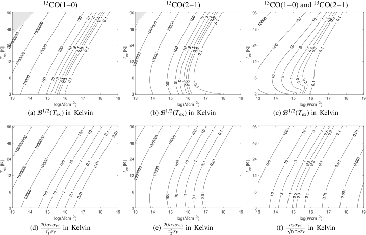
As the inversion of the Fisher matrix is done numerically, we do not have a simple explicit expression of the CRBs. In this section, we thus empirically analyze their evolution as a function of the physical properties of the analyzed medium in a particular case taken from the ORION-B project. To generate figures 2, 3, and 4, we assume that the two measured lines are ${}^{13}\mathrm{CO}$(1$-$0) and ${}^{13}\mathrm{CO}$(2$-$1). The two corresponding opacities are noted $\tau_{1}$ and $\tau_{2}$. The number of samples is $K=80$ for each line at a spectral resolution of $0.5\mathrm{\,km\,s^{-1}}$. Only one velocity component is assumed in the remainder of this section. The amount of noise is fixed and identical for both lines at $\sigma_{b,1}=\sigma_{b,2}=100\mathrm{\,mK}$.

The values of the Cramer-Rao Bounds of the unknown parameters (i.e., $T_{\mathrm{ex}}$, $\log N$, $\Delta_{V}$ and $\sigma_{V}$) are then computed as a function of the values of $T_{\mathrm{ex}}$ and $N$. The Fisher matrices are computed following Eq. (14), and then numerically inverted to obtain ${\cal B}(\theta_{i})=[\boldsymbol{I}_{F}^{-1}]_{ii}$. The excitation temperature $T_{\mathrm{ex}}$ is sampled logarithmically between $3\mathrm{\,K}$ and $99\mathrm{\,K}$, the column density $N$ is sampled logarithmically between $10^{13}\mathrm{\,cm^{-2}}$ and $10^{19}\mathrm{\,cm^{-2}}$, and the other two parameters are kept constant at $\Delta_{V}=1.1\mathrm{\,km\,s^{-1}}$ and $\sigma_{V}=0.61\mathrm{\,km\,s^{-1}}$ (arbitrarily chosen). This leads to figures 2, 3, and 4, where $N$ and $T_{\mathrm{ex}}$ varies horizontally, and vertically, respectively. In these figures, the variations of ${\cal B}^{1/2}(\theta_{i})$ are shown instead of the variations of ${\cal B}(\theta_{i})$ because the square root of the CRB is homogeneous to the estimation standard deviation. It can thus be interpreted as errorbars on the estimated parameter $\theta_{i}$. Varying $T_{\mathrm{ex}}$ and $N$ changes not only the signal-to-noise ratio, but also the amount of information measured by the Fisher matrix because of the non linearity in the radiative transfer equation.

4.4 Precision of the estimation of the centroid velocity $\Delta_{V}$ and the associated velocity dispersion $\sigma_{V}$

Figure 2(a-b) shows variations of ${\cal{B}}^{1/2}(\Delta_{V})$ and ${\cal{B}}^{1/2}(\sigma_{V})$. For $N\geq 10^{16}\mathrm{\,cm^{-2}}$ and $T_{\mathrm{ex}}\geq 12\mathrm{\,K}$, the square root of both CRBs are smaller than $0.01\mathrm{\,km\,s^{-1}}$. This means that any efficient unbiased estimator will have a small dispersion around the actual values. This can be written $\widehat{\Delta}_{V}=1.10\pm 0.01\mathrm{\,km\,s^{-1}}$ and $\widehat{\sigma}_{V}=0.61\pm 0.01\mathrm{\,km\,s^{-1}}$.

Figure 2(c) shows a function of $K{\cal R}$, where ${\cal R}$ is the signal-to-noise ratio defined by

$${\cal R}=\frac{\sum_{n=1}^{K}(s_{n,1}^{2}+s_{n,2}^{2})}{K(\sigma_{b,1}^{2}+\sigma_{b,2}^{2})}.$$ (19)

This expression is used in signal processing to quantify the signal-to-noise ratio on the “energy” of the signal. In our case, we empirically find that, as a rule of thumb

$${\cal{B}}^{1/2}(\Delta_{V})\simeq{\cal{B}}^{1/2}(\sigma_{V})\simeq\frac{1.5\sigma_{V}}{\sqrt{2K{\cal R}}}.$$ (20)

While the dependency on $\sigma_{V}$ is not presented in Fig. 2, we checked that Eq. (20) remains valid when $\sigma_{V}=0.3$, $1.31$, and $2\mathrm{\,km\,s^{-1}}$. The estimation precision on $\Delta_{V}$ and $\sigma_{V}$ depends on the signal-to-noise ratio and on $\sigma_{V}$. This is expected because of the similarity with the problem of delay estimation in radar for which le Chevalier (1989) obtained an analytic formulation similar to Eq. (20).

4.5 Precision of the estimation of the excitation temperature $T_{\mathrm{ex}}$

In this section, we start to quantitatively evaluate the gain in precision when two lines are observed instead of a single one. Figure 3 compares the variations of ${\cal{B}}^{1/2}(T_{\mathrm{ex}})$ when only ${}^{13}\mathrm{CO}$(1$-$0) or ${}^{13}\mathrm{CO}$(2$-$1) is available to constrain the excitation temperature, and when both lines are available. To interpret this figure, we first mention that, for low column densities, the uncertainty quickly increases leading to large values of the CRB, especially for $N<10^{16}$ cm^-2. While the variation of the CRB as a function of the excitation temperature for a given column density is monotonous in the considered range for the ${}^{13}\mathrm{CO}$(1$-$0) line, it shows a different behaviour for the ${}^{13}\mathrm{CO}$(2$-$1) line, with a minimum near 6 K, and an increase of the CRB for lower values of the excitation temperature. This different behaviour is related to higher energy of the upper state of the $2-1$ transition. The emerging ${}^{13}\mathrm{CO}$(2$-$1) signal, which is proportional to the population of the upper level of the transition, approaches zero and becomes close to the noise level.

For the considered example, the analysis of a single line (see Fig. 3 (a-b)) will give a reference precision on $T_{\mathrm{ex}}$ of $0.1\mathrm{\,K}\leq{\cal{B}}^{1/2}(T_{\mathrm{ex}})<10\mathrm{\,K}$ for typically $N>[10^{16}\,-\,10^{17.5}]\mathrm{\,cm^{-2}}$. The dependence on $T_{\mathrm{ex}}$ is such that the same CRB is also reached at higher column densities for higher values of $T_{\mathrm{ex}}$. This behavior of the CRB can be qualitatively understood as resulting from the increase of the line opacity. When the opacity becomes larger than about 3, the peak temperature only depends on $T_{\mathrm{ex}}$ as the factor $[1-\exp(-\Psi(\nu_{l}^{cent}))]$ in Eq (4) approaches unity. The CRB almost linearly depends on $\log T_{\mathrm{ex}}$ above $6\mathrm{\,K}$. The analysis of two lines (see Figure 3c) greatly improves the situation. One reaches the same precision on $T_{\mathrm{ex}}$ for column densities that are between one and two orders of magnitude lower, i.e., $0.1\mathrm{\,K}\leq{\cal{B}}^{1/2}(T_{\mathrm{ex}})<10\mathrm{\,K}$ for typically $N>[10^{14}\,-\,10^{16.5}]\mathrm{\,cm^{-2}}$. Here again the precision almost linearly depends on $\log T_{\mathrm{ex}}$ above $6\mathrm{\,K}$.

The second row of Figure 3 shows functions of the opacities. Trying for several values of $\sigma_{V}$, we empirically obtain

$${\cal{B}}^{1/2}(T_{\mathrm{ex}})\simeq\frac{20\,\sigma_{b}\,\sigma_{V,0}}{\tau_{l}^{2}\,\sigma_{V}},$$ (21)

when a single line is available, either ${}^{13}\mathrm{CO}$(1$-$0) or ${}^{13}\mathrm{CO}$(2$-$1). In this equation, $\sigma_{V,0}=1\mathrm{\,km\,s^{-1}}$ is a constant fixed so that the expression depends on $\sigma_{V}$, but remains homogeneous to a temperature. When these two lines are available, we obtain

$${\cal{B}}^{1/2}(T_{\mathrm{ex}})\simeq\frac{\sigma_{b}\,\sigma_{V,0}}{\sqrt{\tau_{1}\tau_{2}}\,\sigma_{V}}.$$ (22)

Hence, according to Eq. (21) and Eq. (22), when opacities are close to one, the gain in precision (in standard deviation) is around 20 when one observes two lines of the same species instead of a single one. These relations suggest that the parameters that control the difficulty of the estimation problem are the amount of noise $\sigma_{b}$, the velocity dispersions $\sigma_{V}$, and the opacities.

Figure 5: Illustration of the correlation between $N$ and $\sigma_{V}$ estimations when a single line (${}^{13}\mathrm{CO}$(1$-$0)) is available. The blue points in the scatter plots show the estimations of $N$ and $\sigma_{V}$ obtained with a Monte Carlo simulation of individual spectra that share the same physical parameters and different realizations of a white Gaussian noise with standard deviation $\sigma_{b}=100\mathrm{\,mK}$. The parameters are $T_{\mathrm{ex}}=18\mathrm{\,K}$, $N=10^{17.5}\mathrm{\,cm^{-2}}$, $\Delta_{V}=1.1\mathrm{\,km\,s^{-1}}$, and $\sigma_{V}=0.61\mathrm{\,km\,s^{-1}}$.

Figure 6: Noise standard deviation $\sigma_{b,\rho}$ in $\mathrm{\,mK}$ which ensures that relative precisions are better than $\rho\%$ (for details see Eq. (25)). Top: A single line is analyzed. Bottom: Two lines ${}^{13}\mathrm{CO}$(1$-$0) and ${}^{13}\mathrm{CO}$(2$-$1) are analyzed. The contours for 10 and 100$\mathrm{\,mK}$ are highlighted because these $\sigma_{b}$ values bracket the values reached during typical observations at the IRAM-30m. For this analysis, $\Delta_{V}$ is fixed at 1.1$\mathrm{\,km\,s^{-1}}$, but the computations are done for four different values of $\sigma_{V}$ (0.3, 0.6, 1.3, and 2.0$\mathrm{\,km\,s^{-1}}$) and then projected on the $(N,T_{\mathrm{ex}})$ plane (see text for details).

Figure 7: Same as Figure 6, except that the contours show the variations of the peak-signal-to-noise ratio, ${\cal P}_{\rho}$, required to reach a given relative accuracy $(\rho\%)$.

4.6 Precision of the estimation of the column density $N$

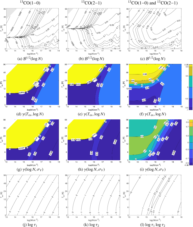
The top row of Fig. 4 shows that the precision on the estimation of $N$ has a complex behavior when only one line is available. To interpret this, we note that even efficient estimators of $\boldsymbol{\theta}$ have correlated components described by the correlation coefficients of the Fisher matrix. The correlation coefficient between $T_{\mathrm{ex}}$ estimations and $\log N$ estimations is given by

$$\gamma(T_{\mathrm{ex}},\log N)=\frac{{\cal{B}}(T_{\mathrm{ex}},\log N)}{{\cal{B}}^{1/2}(T_{\mathrm{ex}}){\cal{B}}^{1/2}(\log N)},$$ (23)

where ${\cal{B}}(T_{\mathrm{ex}},\log N)=[\boldsymbol{I}_{F}^{-1}]_{12}$ is the non-diagonal element of the inverse Fisher matrix, see Eq. (14). We also introduce the correlation coefficient between $\log N$ estimations and $\sigma_{V}$ estimations

$$\gamma(\log N,\sigma_{V})=\frac{{\cal{B}}(\log N,\sigma_{V})}{{\cal{B}}^{1/2}(\log N){\cal{B}}^{1/2}(\sigma_{V})}$$ (24)

where ${\cal{B}}(\log N,\sigma_{V})=[\boldsymbol{I}_{F}^{-1}]_{24}$, see Eq. (14).

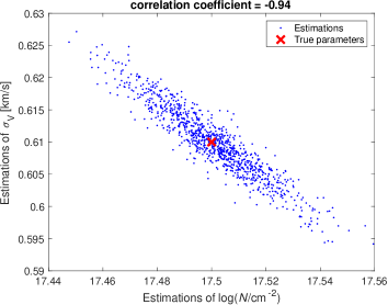
Correlation coefficients are built such that their value ranges from -1 to 1. As long as $|\gamma|<1$, CRBs remain finite and thus estimating parameters usually remains possible. There is a complete ambiguity between estimations of the pairs ($T_{\mathrm{ex}}$ and $\log N$) or ($\log N$ and $\sigma_{V}$), only when values of $|\gamma|=1$. In this case, the variance of these estimations becomes infinite. Figure 5 shows a simulated example where $\log(N)$ and $\sigma_{V}$ can be accurately estimated even though they are highly (but not completely) anti-correlated. Starting from a modeled spectrum with $\log(N/\mathrm{\,cm^{-2}})=17.5$, $\sigma_{V}=0.61$$\mathrm{\,km\,s^{-1}}$, and $T_{\mathrm{ex}}=18\mathrm{\,K}$, we built one thousand realizations of the observed spectrum with a Monte Carlo simulation, and we fitted the LTE model using the estimator proposed in Sect. 5.1. This Monte Carlo simulation allows us to numerically estimate the standard deviation on the estimated parameters and the correlation coefficient between $\log(N)$ and $\sigma_{V}$. This coefficient is -0.94, implying that the parameters are highly anti-correlated. However, the standard deviation on the $\log(N/\mathrm{\,cm^{-2}}$ and $\sigma_{V}$ estimations are 0.017 and $0.005\mathrm{\,km\,s^{-1}}$, respectively. This corresponds to typical relative errors of 4.0 and 0.8%, respectively. Hence some high (anti-)correlation does not necessarily imply that the model parameters can not be estimated, in contrast with a widespread intuition. While we illustrated this property with a given estimator, this statement is true for the CRB analysis. This emphasizes another of its interests. It provides standard deviations and coefficient of correlations without requiring to implement any Monte Carlo simulation.

The second and third row of Fig. 4 show important ambiguities (i.e., correlation coefficients close to one or minus one) between estimations of $\log N$ and $T_{\mathrm{ex}}$ and even more ambiguities between estimations of $\log N$ and $\sigma_{V}$ (in particular for large values of $N$). When a single line is observed (Fig. 4 d e, g, h), $|\gamma(T_{\mathrm{ex}},\log N)|$ and $|\gamma(\log N,\sigma_{V})|$ are mostly larger than 0.9 for small $N$ (in Fig. 4 d-e yellow pixels correspond to $\gamma>0.99$ and in g-h to $\gamma>0.9$). For high $N$, the ambiguity with $T_{\mathrm{ex}}$ decreases, but not the one with $\sigma_{V}$ (in Fig. 4 d-e light blue values are $-0.5<\gamma<0$ while in Fig. 4 g-h dark blue values correspond to $\gamma<-0.9$ and $\gamma<-0.99$). The horizontal asymptote on the left of the CRB maps corresponds to a very sharp change of sign of correlation coefficients $\gamma$. Figure 4 f and i show that, although some ambiguities remain between $\log N$ and $\sigma_{V}$ for high $N$ and small $T_{\mathrm{ex}}$, having two lines mitigates these ambiguities in most cases.

As a rule of thumb, with a single line (see Fig. 4 a-b), ${\cal{B}}^{1/2}(\log N)<0.1$ for $N>[10^{16}\,-\,10^{17}]\mathrm{\,cm^{-2}}$ (depending on $T_{\mathrm{ex}}$), and $T_{\mathrm{ex}}\geq[6-12]\mathrm{\,K}$ (depending on $N$). With two lines (Fig. 4 c), the situation greatly improves: ${\cal{B}}^{1/2}(\log N)<0.1$ for $N>[10^{15}\,-\,10^{17}]\mathrm{\,cm^{-2}}$ (depending on $T_{\mathrm{ex}}$) and $T_{\mathrm{ex}}\geq 6\mathrm{\,K}$. Figures 4 a, b, c also show local minima of the ${\cal{B}}^{1/2}(\log N)$ when $T_{\mathrm{ex}}$ increases and $N\geq 10^{17}\mathrm{\,cm^{-2}}$, and when $N$ increases and $T_{\mathrm{ex}}\geq 6\mathrm{\,K}$. To interpret these, the last row of Fig. 4 shows functions of the opacities. Comparing these with the variations of ${\cal{B}}^{1/2}(\log N)$ shows that the smallest values of ${\cal{B}}^{1/2}(\log N)$ (i.e., the best achievable precision) are mainly located at the area where $\tau_{1}$ and $\tau_{2}$ are close to 1. With two lines (see Fig. 4l), the best precision is when $\tau_{1}<1$ and $\tau_{2}>1$.

4.7 Maximum noise tolerable to get a given relative precision on the different parameters

In the previous section, the standard deviation of the noise $\sigma_{b}$ was fixed to $100\mathrm{\,mK}$. Conversely, we now derive the amount of noise that guarantees a given relative CRB precision for $T_{\mathrm{ex}}$, $\log N$, $\sigma_{V}$ and $\Delta_{V}$. We compute $\sigma_{b,\rho}$ the maximal value of $\sigma_{b}$ that satisfies the following inequalities

$$\begin{array}[]{cc}{\cal{B}}^{1/2}(T_{\mathrm{ex}})/T_{\mathrm{ex}}\leq\rho,&{\cal{B}}^{1/2}(\log N)\leq\rho,\\ {\cal{B}}^{1/2}(\sigma_{V})/\sigma_{V}\leq\rho,&{\cal{B}}^{1/2}(\Delta_{V})/\sigma_{V}\leq\rho,\end{array}$$ (25)

where $\rho$ is a fixed threshold. In other words, instead of analyzing the precision for a given amount of noise, one can also analyze the tolerable level of noise to ensure an intended precision (herein described by $\rho$). Such an analysis will be useful to design an observation program and optimize the telescope time needed to reach the scientific goal.

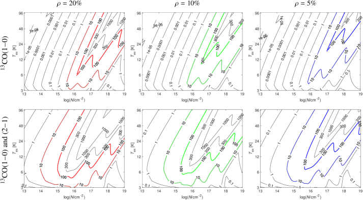
Up to this point of the paper, we checked the variations of the quantities as a function of $T_{\mathrm{ex}}$ and $N$ with fixed values of $\Delta_{V}$ and $\sigma_{V}$. Figure 6 shows the variations of $\sigma_{b,\rho}$ as a function of $T_{\mathrm{ex}}$ and $N$. As the computation of $\sigma_{b,\rho}$ includes the computation of maximum values, it is possible to make the computations in three dimensions (with varying values of $T_{\mathrm{ex}}$, $N$, and $\sigma_{V}$), and to project these on the $(T_{\mathrm{ex}},N)$ plane. That is what is shown in Fig. 6 for different values of the relative precision $\rho$ (5, 10, and 20%).

The IRAM-30m time estimator for the EMIR receivers indicates that we can achieve a sensitivity of 100 mK in $30$ to $120\mathrm{\,s}$ at 110 and 220 GHz for a spectral resolution of 0.5$\mathrm{\,km\,s^{-1}}$. Similarly, we can achieve a sensitivity of 10 mK in 1 to 3 hours depending on the frequency and the observing mode (frequency or position switching). The colored contours thus correspond to the “fast/slow” acquisition mode at the IRAM-30m. The comparison between the top and bottom lines allows us to see the gain in precision when analyzing the two lowest $J$ lines of ¹³CO instead of a single one. In particular, the surface of reachable combinations of column density and excitation temperature more than doubles when analyzing two lines.

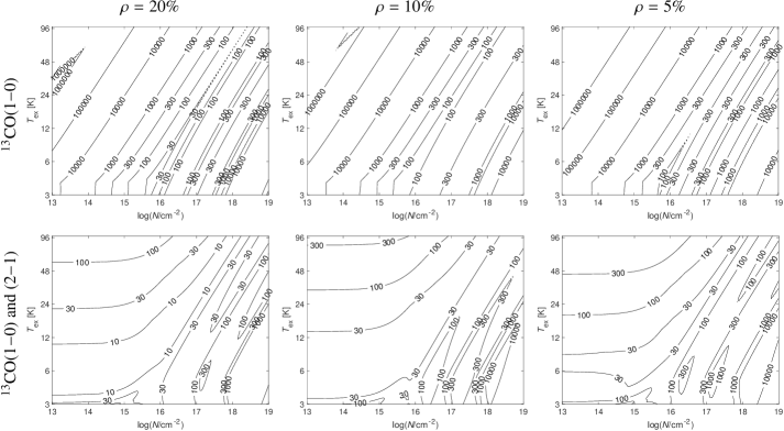
Instead of analyzing the level of noise, one can also analyze the peak-signal-to-noise ratio defined for one transition $l$ by

$${\cal P}_{l}=\frac{\max_{n}s_{n,l}}{\sigma_{b,l}}$$ (26)

and for two transitions by ${\cal P}=\max_{l=1,2}{\cal P}_{l}$. Figure 7 shows the variations of minimum peak-signal-to-noise ratio ${\cal P}_{\rho}$ for similar conditions as in Fig. 6. Analyzing only the ${}^{13}\mathrm{CO}$(1$-$0) line requires at least a signal-to-noise ratio of 100 to get a relative precision of 20%. Adding the ${}^{13}\mathrm{CO}$(2$-$1) line in the analysis reduces the minimum signal-to-noise ratio by a factor up to 10 to reach the same relative precision. The required signal-to-noise ratio increases at high column densities because the lines become optically thick, and at a combination of low column density and high excitation.

4.8 How to complement ${}^{12}\mathrm{CO}$(1$-$0) observations?

All the previous analyses were done for the ¹³CO isotopologue because it enabled us to study the case of low $J$ lines that experience the transition from optically thin to thick regime over the range of column densities and excitation temperatures that are found in molecular clouds. However, the targeted transition when observing the molecular gas of a new astronomical source is usually ${}^{12}\mathrm{CO}$(1$-$0) because it is the strongest line in the easily observable 3mm atmospheric window (Wilson et al., 1970; Pety et al., 2017).

Figure 8: Noise standard deviation $\sigma_{b,\rho}$ in $\mathrm{\,mK}$ which ensures relative precisions better than 20% when a single line of ¹²CO is analyzed. Other details are identical to Fig. 6.

Figure 9: Noise standard deviation $\sigma_{b,\rho}$ in $\mathrm{\,mK}$ which ensures relative precisions better than 20% when a couple of ¹²CO lines are observed: $J=1-0$ and a higher $J$ line. Other details are identical to Fig. 6.

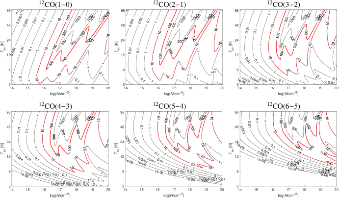
We here ask two questions. First, what is the best $J$ line to observe to reach a relative precision of 20% on all the estimated parameters? Figure 8 shows the variations of the maximum noise $\sigma_{b,\rho}$ when a single line is observed among the first six rotational transitions of ¹²CO. A global pattern is seen, especially for the higher energy transitions ${}^{12}\mathrm{CO}$(4$-$3), ${}^{12}\mathrm{CO}$(5$-$4), ${}^{12}\mathrm{CO}$(6$-$5), For instance, if $N$ lies in the interval $[10^{17},\,10^{19}]\mathrm{\,cm^{-2}}$ and $T_{\mathrm{ex}}>24\mathrm{\,K}$, the ${}^{12}\mathrm{CO}$(6$-$5) line seems the best choice (from a CRB point of view) because it allows to reach $20\%$ accuracy over this broad range of parameters for a noise level of 100 mK. However this line is not easy to access from ground based telescopes because of the limited atmospheric transmission at the line frequency of 690 GHz.

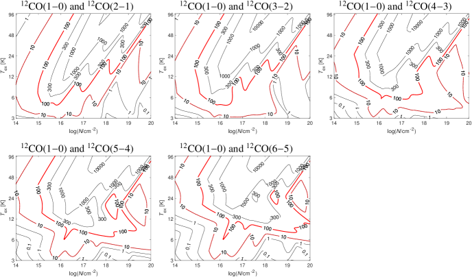
Second, what is the best $J$ line to be observed to complement the $J=1-0$ line to reach the same relative precision of $20\%$? Figure 9 seems to indicate that observing ${}^{12}\mathrm{CO}$(6$-$5) would be the most useful as it would allow to tolerate a noise level of $\sigma_{b}=300\mathrm{\,mK}$ and keep a good precision for $N$ in the interval $[10^{16.0},\,10^{18.5}]\mathrm{\,cm^{-2}}$. We stress that this result only applies to the case where all transitions have the same excitation temperature. In practice, deviations from a Boltzmann population may be present leading to different excitation temperatures for the ¹²CO transitions (van der Tak et al., 2007) because of the higher critical densities of the higher-$J$ transitions. Nevertheless, the usefulness of mildly excited lines remains valid. Non-LTE approaches will be developed in the future that will provide a quantitative assessment of the diagnostic power of these lines.

5 Application to the ORION-B data

The CRB is only a lower bound on the variance of any unbiased estimator. Once the order of magnitude of the CRBs have been analyzed, the next step is to find a good estimator of physical parameters. In this section, we first propose such an estimator and analyze its performance for a realistic amount of noise (herein chosen to $\sigma_{b}=100\mathrm{\,mK}$), before applying it to the ORION-B data.

5.1 Proposed estimator

The maximum likelihood estimator (MLE) is a good candidate because under mild conditions, it reaches the CRB asymptotically, i.e., when $\sigma_{b}\mapsto 0$ (Garthwaite et al., 1995). Appendix B details the computation of this estimator, its initialization, and the iterative algorithm used to yield the estimation that is noted $\widehat{}\boldsymbol{\theta}$. We also briefly discuss its computational efficiency.

Appendix C analyzes the performance of the proposed estimator on simulated data. This appendix shows that this estimator performs optimally for pairs of $(T_{\mathrm{ex}},N)$ values such that a relative precision of reference is reached for all estimated parameters (i.e., the conditions of Eqs. (25) are satisfied with $\rho=20\%$). Interestingly, this appendix also shows that the obtained estimation $\widehat{}\boldsymbol{\theta}$ can be injected in the CRB computation to detect whether or not this estimation is accurate.

5.2 Estimation of the number of velocity components and initialization of the parameters

The number of velocity components is a priori unknown. While we could have tried to use our maximum likelihood estimator to fit the data with either one or two components, we would then have had to devise a statistical test to determine which assumption to choose. Instead, it is simpler to check for the presence of several local maxima in the spectrum denoised with ROHSA, the technique mentioned in Sect. 2. In particular, this allows us to have a spatially coherent detection of the number of components. The ROHSA algorithm is applied separately on the ${}^{13}\mathrm{CO}$(1$-$0), $\mathrm{C}^{18}\mathrm{O}$(1$-$0), and ${}^{12}\mathrm{CO}$(1$-$0) lines. If one of the denoised spectra for ${}^{13}\mathrm{CO}$(1$-$0), $\mathrm{C}^{18}\mathrm{O}$(1$-$0) or ${}^{12}\mathrm{CO}$(1$-$0) has at least two local maxima in the velocity interval of interest $[8.25,14.25]\mathrm{\,km\,s^{-1}}$, we then fix the number of velocity components to two for all three species. The denoised spectra ${}^{13}\mathrm{CO}$(1$-$0), $\mathrm{C}^{18}\mathrm{O}$(1$-$0) and ${}^{12}\mathrm{CO}$(1$-$0) are analyzed iteratively in this order, and as soon as two components are selected based on one of the three spectra, the velocities associated to the local maxima are used to initialize the estimations of the velocity $\Delta_{V}$ of each component for all three species. This ensures that the velocities of each component will stay compatible for all three species during the fit. We analyze the denoised spectra in the above order because the ${}^{13}\mathrm{CO}$(1$-$0) line has both a good signal-to-noise ratio, and moderate opacities. The $\mathrm{C}^{18}\mathrm{O}$(1$-$0) line delivers a good information on the underlying velocity structure because it is most often optically thin, but its limited signal-to-noise ratio may hamper the $\Delta_{V}$ initialization. The saturation that happens for the ${}^{12}\mathrm{CO}$(1$-$0) line also makes the determination of the $\Delta_{V}$ initializations inaccurate. Finally, when all the three denoised spectra have only one maximum, one component is independently fitted per species.

When initializing the parameters before maximizing the likelihood, we use two different assumptions to help the algorithm to converge towards reasonable solutions. First, when two components are detected, we use the same $\Delta_{V}$ and $\sigma_{V}$ initializations for all the species so that the estimated parameters for each component remain correctly paired among the three species, as explained above. The white contours in Fig. 13 delimit the regions where two local maxima have been detected. Only $23\%$ of the field of view requires two velocity components. As the estimations of $T_{\mathrm{ex}}$, $N$, and $\sigma_{V}$ are highly correlated (see Sect. 4.6), we systematically search in the 3D grid described in Sect. B.2 to initialize them. We stress that this is only during the initialization process that we use the same values $\Delta_{V}$ and $\sigma_{V}$ for ${}^{13}\mathrm{CO}$ and $\mathrm{C}^{18}\mathrm{O}$. The maximization of the log-likelihood is done independently on each species, ensuring that the estimations of $\Delta_{V}$ and $\sigma_{V}$ may take a different value for each species.

Second, a single line of ¹²CO is available and it is quite optically thick. In our analysis of the CRB, we observed in Figure 4 (d-e and g-h) that the estimation of $\log N$ is highly correlated with $\sigma_{V}$, when $N$ is high. This may imply some degeneracy between the estimation of the velocity dispersion and the column density. To alleviate this issue, we first deal with ${}^{13}\mathrm{CO}$(1$-$0), ${}^{13}\mathrm{CO}$(2$-$1), $\mathrm{C}^{18}\mathrm{O}$(1$-$0), $\mathrm{C}^{18}\mathrm{O}$(2$-$1), and we use the estimation of $\sigma_{V}$ obtained on ¹³CO to fix $\sigma_{V}$ for the estimation of the other parameters ($T_{\mathrm{ex}}$, $\log N$ and $\Delta_{V}$) in the analysis of the ${}^{12}\mathrm{CO}$(1$-$0) line. If this assumption is false, the obtained estimations of the other parameters will be biased. While this procedure is not ideal, we empirically obtained estimations of $T_{\mathrm{ex}}$ and $\log N$ much closer to physical intuition: in particular, the estimations of the column density are 100 times too large when all four parameters are estimated. An analysis of the impact of a potential incorrect value of $\sigma_{V}$ goes beyond the scope of the present paper.

Figure 10: Two examples of LTE fit of the CO isotopologues lines. In the titles, $T_{\mathrm{ex}}$ is expressed in Kelvin, $N$ in cm^-2, $\Delta_{V}$ in $\mathrm{km\,s^{-1}}$, and $\sigma_{V}$ in $\mathrm{km\,s^{-1}}$. The plain lines show the data, and the dotted ones show the fit results. Values in red indicate estimations whose relative precision is larger than 20%. The associated lines of sight can be localized in Fig. 1 (see red crosses).

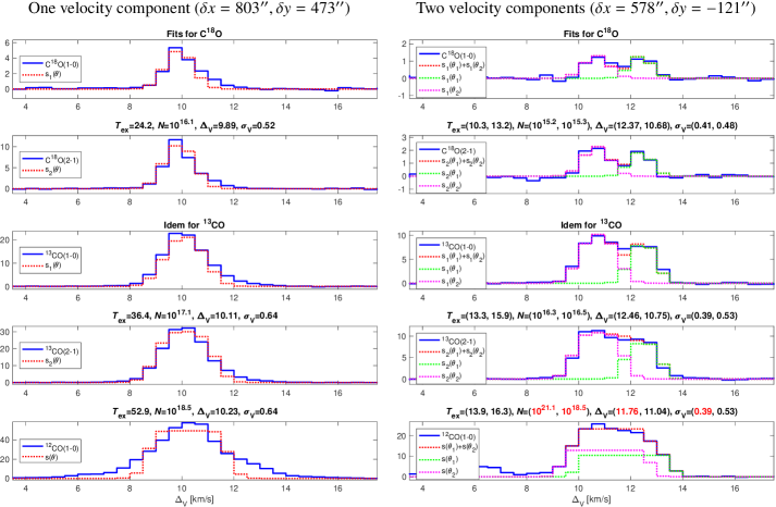
5.3 Detailed analysis of two lines of sight

Figure 10 shows how the proposed estimator succeeds to fit the C¹⁸O, ¹³CO and ¹²CO low $J$ lines towards two lines of sight in the studied field of view (see red crosses Fig. 1), at offsets $(803^{\prime\prime},473^{\prime\prime})$ and $(578^{\prime\prime},-121^{\prime\prime})$. The spectra on the left column are modeled with a single velocity component but they are asymmetric. This implies that our model is not perfectly adequate because it assumes that the line profile is symmetric. The issue is most problematic for ¹²CO, because the high opacity and the complex underlying velocity field imply a more complex profile with broad wings on each side of the line. A detailed solution for this issue is beyond the scope of the present paper.

The spectra on the right column are well fitted with two different velocity components. The estimations for the C¹⁸O and ¹³CO species are physically relevant because the two velocity components are well separated in velocity. This is less obvious for ¹²CO, which presents a large velocity overlap of the two components.

5.4 Estimation of the quality of the fit and filtering out inaccurate estimations

In this section, we first compute the “energy” and the standard deviation of the fit residuals as two ways to quantify the quality of the fit. We then explain how we will filter out inaccurate estimations from the physical analysis.

After a fit, we can define three different “energies” in the sense of the information theory.

• The “energy” of the measured signal is

  $${\cal E}_{x_{l}}=\sum_{n}x_{n,l}^{2}.$$ (27)

• The “energy” of the estimated signal is

  $$\begin{array}[]{ccc}{\cal E}_{s_{l}}=\sum_{n}s^{2}_{n,l}(\widehat{}\boldsymbol{\theta})&\text{or}&{\cal E}_{s_{l}}=\sum_{n}s^{2}_{n,l}(\widehat{}\boldsymbol{\theta}_{1})+s^{2}_{n,l}(\widehat{}\boldsymbol{\theta}_{2}),\end{array}$$ (28)

  depending of the number of estimated components.

• The “energy” of the fit residual is

  $${\cal E}_{r_{l}}=\sum_{n}r_{n,l}^{2},$$ (29)

  $$\begin{array}[]{ll}\text{where}&r_{n,l}=x_{n,l}-s_{n,l}(\widehat{}\boldsymbol{\theta}),\\ \text{or}&r_{n,l}=x_{n,l}-s_{n,l}(\widehat{}\boldsymbol{\theta}_{1})-s_{n,l}(\widehat{}\boldsymbol{\theta}_{2}).\end{array}$$ (30)

All the sums are computed on an interval of $10\mathrm{\,km\,s^{-1}}$ around the maximum. The fit quality can then be quantified by comparing the “energy” in the residual with either the “energy” in the observed spectrum $({\cal E}_{r_{l}}/{\cal E}_{x_{l}})$ or the difference of “energy” between the observed and estimated signals $(\{{\cal E}_{x_{l}}-{\cal E}_{s_{l}}\}/{\cal E}_{x_{l}})$. The former formula tells us the fraction of the observed “energy” that has not been fitted. The latter formula tells us whether the observed spectra has been under-fitted (positive value) or over-fitted (negative value). Measuring the residual “energies” is similar to computing a $\chi^{2}$ in least-square fitting. Another way to quantify the quality of the fit is to compare the standard deviation of the residuals $\sigma_{r}=\left(\frac{1}{K-1}\sum_{n}r_{n,l}^{2}\right)^{1/2}$ with the noise standard deviation $(\sigma_{b})$ on the observed spectrum. The fit is good when $\sigma_{r}\sim\sigma_{b}$.

We can in addition use the CRB framework to filter out pixels with inaccurate estimations. As explained in Sect. C.1, an estimation will be considered inaccurate when there is at least one estimation among the $3\times 3$ neighboring pixels, for which at least one of the following conditions is satisfied

$$\begin{array}[]{ll}{{\cal{B}}}^{1/2}(\widehat{T}_{\mathrm{ex}})/\widehat{T}_{\mathrm{ex}}>0.2,&{{\cal{B}}}^{1/2}(\log\widehat{N})>0.2,\\ {{\cal{B}}}^{1/2}(\widehat{\sigma}_{V})/\widehat{\sigma}_{V}>0.2,&{{\cal{B}}}^{1/2}(\widehat{\Delta}_{V})/\widehat{\sigma}_{V}>0.2.\end{array}$$ (31)

Figure 11: Joint histograms of the standard deviations of the residuals $(\sigma_{r})$ and of the noise $(\sigma_{b})$ for all the studied lines. Standard deviations are expressed in Kelvin. The dashed lines correspond to ratios 1 and 10.

Figure 12: Spatial variations of the observed spectrum “energy” (a), of the residual “energy” (b), of their ratio in % (c), and of the ratio of “energy” in % that has not been modeled (d). The unit of the color look-up table is Kelvin². White contours show the regions where two components have been detected.

5.5 Global analysis of the quality of the estimation

Figure 11 compares the standard deviation of the residuals $(\sigma_{r})$ with the standard deviation of the noise $(\sigma_{b})$ for all the lines studied here. If the fits were ideal, the joint histograms would only peak near a line of slope one. They thus suggest that the C¹⁸O lines are better fitted than the ¹³CO lines, and that the ¹²CO lines are the least well fitted. We also checked that the residuals are larger (i.e., $\sigma_{r}>\sigma_{b}$) when the energy ${\cal E}_{x}$ is large (not shown in the figure). As the signal-to-noise ratio also increases with ${\cal E}_{x}$, this issue implies some misspecification of the model. The best fit happens for the C¹⁸O(1-0) line that has the lowest opacity. In that case, the profiles $\Psi$ are almost perfect Gaussian profiles. On the contrary the high opacity of the ¹²CO(1-0) line implies that the profiles are highly saturated, and any small kinematic perturbations will create deviations from a Gaussian profile as shown in Fig. 10, where the asymmetry pattern could not be taken into account by the model. A better modeling could thus require additional velocity components especially for the ${}^{12}\mathrm{CO}$(1$-$0) line. Another limit of the model is that it does not encode self-absorption signatures that may happen at large opacity.

Figures 12 a and b show the spatial distributions of the “energy” of the observed spectra and of the fit residuals for the ${}^{13}\mathrm{CO}$(1$-$0) line. Both images share the same color look-up table. On the left image, the yellow pixels correspond to bright molecular gas while the blue pixels corresponds to faint signal or noise associated with the IC 434 Hii region. The “energy” of the residual still exhibits spatially coherent structures, but at a much smaller level than the “energy” of the measured spectra. Our estimator under-fits the observed spectra as shown in Fig. 12d. This may be related to the fact that our model does not fit asymmetric profiles. However, the fit quality is good as illustrated by the image of the energy ratio, which shows that the residual “energy” amounts to less than 1% of the signal (the dark blue color corresponds to 0.01% in image 12c) except in regions where the signal-to-noise ratio becomes small. Figure 23 shows the same quantities for all the lines modeled in this paper. Overall, the fitting method is able to recover all the emission with differences at the percent level or less for all lines.

Increasing the complexity of the line profile model to address the observed misspecifications could be hazardous. While the increase of the number of parameters in more complex models certainly allows one to decrease the difference between the observed spectrum and the model, it may also increase the variance of estimations in such proportions that obtained estimations may become useless. In other words, the simple model used here does not capture all the complexity of the physical processes, but it at least allows us to capture the processes that it already encodes. The fact that the residuals are smaller than $1\%$ compared to the observed signal is sufficient to make the analysis of the excitation temperature, the column density, and the velocity dispersion pertinent for CO isotopologues. The main source of systematic errors in the column density determination results from the deviations from the local thermodynamic equilibrium, leading to a more complex partition function than the simple formula in Eq. (9). The effect is expected to be stronger in warm regions ($T_{\mathrm{ex}}\geq 50-100\mathrm{\,K}$) where many rotational levels are populated and contribute to the partition function. These warm regions occupy a small fraction of the total volume and therefore a bias would not affect the general conclusions. Non-LTE approaches will be developed to assess more quantitatively the magnitude of the effect and to provide recommendations on the best method depending on the molecular lines and the range of physical conditions that are studied.

6 Astrophysical implications

Figure 13: Top: Spatial variations of the estimated physical parameters. From left to right: Centroid velocity, velocity dispersion, excitation temperature, column density, and line opacities. Bottom: Spatial variations of the relative precisions. From left to right: Relative precision on the centroid velocity, velocity dispersion, excitation temperature, column density, and line peak signal-to-noise ratio. The black contours on the peak signal-to-noise-ratio image delimit the regions where ${\cal P}\geq 3$. On all images, red contours delimit the regions where the relative precision is better than 20% for all estimated parameters, and white contours delimit regions where two components have been estimated. In this latter case, the images only show the estimation that is the closest (in terms of centroid velocity $\Delta_{V}$) to its neighboring pixels.

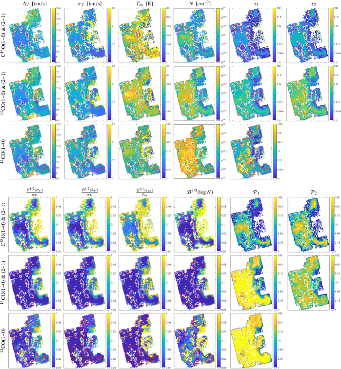
The proposed estimator (see Sect. 5.1) provides accurate column densities, excitation temperatures, and velocity dispersions in the framework of LTE excitation and radiative transfer. This allows us to carefully analyze the errors introduced by the simpler hypotheses that are commonly used for deriving CO isotopologues column densities.

6.1 Estimated parameters and associated uncertainties for C¹⁸O, ¹³CO, and ¹²CO

Figure 14: Comparison between the map of the dust temperature and maps of temperature ratios. Inaccurate estimations are filtered out. The dust temperature is only presented in regions with an accurate estimation of parameters.

Figure 15: Scatter plots between the CO isotopologue excitation temperatures. The color scale encodes the dust temperature $T_{\mathrm{dust}}$. The ellipses represent the interval of confidence for each estimation: Each ellipse is centered on the estimation of the excitation temperature for one pixel and its horizontal and vertical sizes are equal to the associated CRBs. Dashed ellipses correspond to pixels with two components. Inaccurate estimations are filtered out. Dashed red lines show the loci of ratios 1/2, 1, 2, and 4.

Table 2: Statistics of the estimated parameters over all the pixels for the three CO isotopologues.

Quantity	Unit	12CO	13CO	C18O
$T_{\mathrm{ex}}$	K	$30\pm 7.6$	$17\pm 4.6$	$15\pm 4.4$
$T_{\mathrm{ex}}/T_{\mathrm{dust}}$		$1.3\pm 0.3$	$0.76\pm 0.22$	$0.71\pm 0.23$
$\log N$	cm-2	$18\pm 0.5$	$16\pm 0.45$	$15\pm 0.27$
$\log N/N_{\mathrm{H}_{2}}$		$-4.2\pm 0.4$	$-5.6\pm 0.29$	$-6.7\pm 0.15$
$\sigma_{V}$	km s-1	$0.63\pm 0.17$	$0.64\pm 0.26$	$0.58\pm 0.2$
$\log\tau_{1}$		$0.96\pm 0.47$	$-0.06\pm 0.4$	$-0.76\pm 0.25$
$\log\tau_{2}$			$0.34\pm 0.41$	$-0.39\pm 0.25$

Figure 13 shows the spatial variations of the estimated parameters and associated uncertainties for the C¹⁸O, ¹³CO, and ¹²CO isotopologues. Table 2 lists the mean and standard deviation values of the excitation temperatures, column densities, velocity dispersions and opacities. These values are computed over the field of view that is observed for all the lines.

The peak-signal-to-noise ratio of the ${}^{12}\mathrm{CO}$(1$-$0), ${}^{13}\mathrm{CO}$(1$-$0), and ${}^{13}\mathrm{CO}$(2$-$1) lines is large $(>20)$ over most of the studied field of view. The regions where the peak-signal-to-noise ratio of the $\mathrm{C}^{18}\mathrm{O}$(1$-$0) and $\mathrm{C}^{18}\mathrm{O}$(2$-$1) is larger than 20 still amounts to respectively 15% and 32% of the studied field of view. The CRBs are small for all estimated parameters (inside the red contours that delimit the regions where the relative precision is better than 20% for all estimated parameters) except near the regions of transitions between one and two velocity components (i.e., near the white contours). Even though the ¹²CO signal-to-noise ratio is much larger than the C¹⁸O or the ¹³CO one, the ¹²CO estimations are more uncertain (see map of ${\cal B}^{1/2}(\log N)$ for ¹²CO in Figure 13) because a single transition is available and the ¹²CO opacities are large (ranging from 5 to about 1 000). However, the higher signal-to-noise ratio for ¹²CO helps to derive the velocity field in regions where ¹³CO and C¹⁸O are not well detected (diffuse gas).

The largest variations are observed in the column density which varies from the detection limit near 10¹⁵ cm^-2 up to values larger than 10¹⁷ cm^-2 for ¹³CO. The comparison of the column density maps for ¹³CO and C¹⁸O suggests that the C¹⁸O molecules are confined to the high column density regions and avoid the cloud edges. The ¹²CO isotopologue shows a different behavior with emission extending over most of the imaged field of view and column densities ranging from $\sim 10^{16}$ to $\sim 10^{19}$ cm^-2. These behaviors are related to the difference of opacity of the isotopologues lines. Both ¹³CO lines have moderate opacities across the mapped region, with somewhat higher values for ${}^{13}\mathrm{CO}$(2$-$1) than for ${}^{13}\mathrm{CO}$(1$-$0). The ¹²CO is highly optically thick almost everywhere.

For all CO isotopologues, the excitation temperature presents coherent spatial variations with maximum values near the NGC 2023 star forming region. Even though the C¹⁸O emission is fainter and less extended than that of ¹³CO, both species provide similar kinematics information. The velocity field is spatially regular with well-resolved gradients, for instance in the Horsehead nebula at the bottom right of the map. The velocity dispersion $\sigma_{V}$ ranges from 0.4 to 0.8$\mathrm{\,km\,s^{-1}}$, with values around 0.3$\mathrm{\,km\,s^{-1}}$ in the Horsehead nebula (see also Hily-Blant et al., 2005), and somewhat narrower lines for C¹⁸O than for ¹³CO.

6.2 Excitation temperatures

Figure 16: Plots of the ${}^{13}\mathrm{CO}$ column densities per unit intensity of ${}^{13}\mathrm{CO}$(1$-$0) (top) and ${}^{13}\mathrm{CO}$(2$-$1) (bottom) as a function of the excitation temperature. This plot is done for four values of the ${}^{13}\mathrm{CO}$ column density, and $\sigma_{V}=0.61\mathrm{\,km\,s^{-1}}$.

Table 3: Statistics of ratios of the estimated parameters over all the pixels for the three CO isotopologues. We stress that $\sigma_{V}(^{12}$CO$)$ is fixed to $\sigma_{V}(^{13}$CO$)$.

	13CO/C18O	12CO/13CO
$T_{\mathrm{ex}}/T_{\mathrm{ex}}^{\prime}$	$1.3\pm 0.33$	$1.7\pm 0.39$
$\log(N/N^{\prime})$	$1.2\pm 0.17$	$1.4\pm 0.33$
$\sigma_{V}/\sigma_{V}^{\prime}$	$1.1\pm 0.25$	Fixed to $1$

Simplifying assumptions are often made when analyzing the CO rotational emission. The most usual one is that all isotopologues have the same excitation temperature. It is based on the similarity of the collisional cross sections. Because the opacity of a rotational transition scales with the molecular column density, the differences in abundances translate to different opacities. The main isotopologue (¹²CO) has optically thick lines while the rarer isotopologues (¹³CO and C¹⁸O) have lines either optically thin or with moderate opacities (see, e.g., Ripple et al., 2013). Another assumption for high density regions ($n>10^{5}$   cm^-3 Goldsmith & Langer 1978) is the full thermalization of the lowest CO rotational levels at the temperature measured on dust (i.e., assuming the convergence of the dust and gas temperatures). Both hypotheses have been questioned. Recently, in their clustering analysis of a one square degree map in the Orion B cloud, Bron et al. (2018) have shown that the observed CO isotopologue line intensities and line ratios cannot be explained using these simple hypotheses and that differences in excitation temperatures should be present.

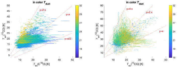
As shown in Fig. 14, the excitation temperatures of the three isotopologues are different across the field of view. The ¹²CO isotopologue has the largest excitation temperature, followed by ¹³CO and C¹⁸O. Table 3 lists the typical ratios of excitation temperatures. They are $T_{\mathrm{ex}}(^{12}$CO$)/T_{\mathrm{ex}}(^{13}$CO$)\sim 1.7$ and $T_{\mathrm{ex}}(^{13}$CO$)/T_{\mathrm{ex}}($C¹⁸O$)\sim 1.3$. Figure 14 shows that these ratios vary significantly as a function of the total column density and dust temperature. Figure 15 suggests that higher dust temperature regions that trace higher UV illumination conditions, tend to show larger differences in excitation temperatures between the CO isotopologues. The same trend is seen when the CO isotopologue excitation temperatures are compared to the dust temperature as in Fig 14. A similar effect has been reported by Welty et al. (2018) for the diffuse/translucent cloud along the line of sight to HD62542.

The excitation temperature of C¹⁸O, which traces the UV shielded regions, is on average lower than $T_{\mathrm{dust}}$ (the mean value of $T_{\mathrm{ex}}/T_{\mathrm{dust}}$ is 0.71, see Table 2). We find a similar situation for ¹³CO(1-0) (mean value $T_{\mathrm{ex}}/T_{\mathrm{dust}}=0.76$), while most of the positions show ¹²CO(1-0) excitation temperatures larger than $T_{\mathrm{dust}}$. This difference between the CO excitation temperature – which is a lower approximation of the gas kinetic temperature– and the dust temperature is indeed expected in photo-dissociation regions and UV-dominated regions where the gas kinetic temperature is larger than the dust temperature. This is different from the usual approximation that $T_{\mathrm{dust}}$ is a good approximation of the gas kinetic temperature in cold and shielded regions.

The difference in excitation temperatures between CO isotopologues can be explained by radiative trapping in the ¹²CO lines or by the presence of kinetic temperature gradients along the line of sight, especially near photodissociation regions, possibly combined with density gradients. Clear spatial patterns emerge in Fig. 14. The C¹⁸O and ¹³CO excitation temperatures get closer to $T_{\mathrm{dust}}$ in regions where $T_{\mathrm{dust}}$ is lower than 20 K. Because the dust emission strongly varies with its temperature (as $T^{(4+\beta)}$ where $\beta$ is the dust emissivity index and takes values between 1.5 and 2, Planck Collaboration XI 2014), the dust temperature derived from a single temperature fit of the spectral energy distribution in lines of sight combining a strongly UV illuminated region and a more shielded material does not represent the conditions in the UV shielded region well. The dust temperature can overestimate the temperature in the shielded gas that represents the bulk of the material. Somehow the illuminated region ”overshines” as compared to the bulk of the matter.

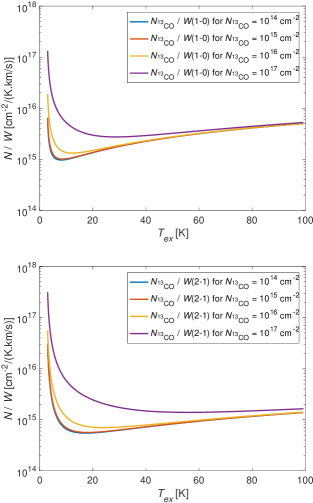
The error introduced in the column density determination by using an incorrect excitation temperature can be estimated by examining the variation of the line column-to-intensity ratio, defined as the ratio of the column density of the species to the line integrated emission, as a function of the excitation temperature. Figure 16 shows the variation of the column-to-intensity ratio for the ${}^{13}\mathrm{CO}$(1$-$0) and ${}^{13}\mathrm{CO}$(2$-$1) lines for different column densities of ${}^{13}\mathrm{CO}$, assuming a velocity dispersion of $0.61\mathrm{\,km\,s^{-1}}$. Column densities of $N_{\mathrm{{}^{13}CO}}\sim 10^{14}-10^{15}\mathrm{\,cm^{-2}}$ correspond to optically thin lines, while the opacity becomes significant (i.e., $\tau\geq 0.5$) for $10^{16}-10^{17}\mathrm{\,cm^{-2}}$. In the optically thin case, the column-to-intensity ratio presents a shallow minimum which depends on the transition, rises rapidly at temperatures lower than the minimum and more slowly for excitation temperatures above the minimum. When the line opacity becomes significant, the shape of the column-to-intensity ratio curve changes and the minimum shifts to higher excitation temperatures or possibly disappears. Therefore, using the ¹²CO excitation temperature for determining the column densities of ¹³CO and C¹⁸O leads to errors in the estimation of these column densities because the associated column-to-intensity ratio is inappropriate. For moderate column densities ($N_{\mathrm{{}^{12}CO}}<10^{16}$ cm^-2), the column densities can be underestimated in the case of low excitation temperatures, or overestimated when using a too high excitation temperature, depending on the position of $T_{\mathrm{ex}}$ relative to the minimum of the column-to-intensity curve. A CO excitation temperature near the minimum of the column-to-intensity curve will minimize the error because a small difference in $T_{\mathrm{ex}}$ in this region will not change the column-to-intensity. For high column densities ($N\sim 10^{17}\mathrm{\,cm^{-2}}$), the bias is significant at low excitation temperatures ($T_{\mathrm{ex}}<20\,K$) because the column-to-intensity ratio (purple curve in Fig. 16) is rising fast at low excitation temperatures.

6.3 Abundances

Figure 17: Comparison of the map of dust-traced H₂ column density with maps of various column density ratios. Inaccurate estimations were filtered out. The dust-traced column density is only presented in regions with an accurate estimation of parameters.

Figure 18: Scatter plot of the CO isotopologue column densities as a function of the dust-traced H₂ column density. Inaccurate estimations are filtered out. The black dashed lines show the expected gas phase abundances relative to H₂ with no depletion: C¹⁸O/H₂ $=5\times 10^{-7}$, ¹³CO/H₂ $=4\times 10^{-6}$, and CO/H₂$=1.4\times 10^{-4}$.

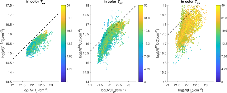
Figure 17 presents maps of the CO isotopologue abundances relative to H₂ (see Sect. 2.2), and Fig. 18 shows scatter plots of the relationships between the CO isotopologue column densities and that of molecular hydrogen. In the mapped area, ¹³CO and ¹²CO can be fitted and analyzed for H₂ column densities larger than $10^{21.5}\mathrm{\,cm^{-2}}$. The threshold for C¹⁸O is about twice higher at $\sim 10^{21.8}\mathrm{\,cm^{-2}}$. Indeed, as shown by Pety et al. (2017) and Orkisz et al. (2019), the threshold for the detection of C¹⁸O is $A_{V}\sim 3\mathrm{\,mag}$ or N(H₂) = $10^{21.5}\mathrm{\,cm^{-2}}$ in the Orion B molecular cloud, while the thresholds for ¹²CO and C¹³O are close to $A_{V}=1$ mag.

Over the mapped area, the mean abundances are well defined at $N(^{13}$CO$)/N($H${}_{2})$ $=10^{-5.6\pm 0.29}=2.5\pm 1.5\times 10^{-6}$, and $N($C¹⁸O$)/N($H${}_{2})$ $=10^{-6.7\pm 0.15}=2.0\pm 0.8\times 10^{-7}$ (see Table 2). These mean abundances are comparable to those of other molecular clouds in the solar neighborhood such as Taurus and Ophiuchus (Frerking et al., 1989). But these values are about a factor of two lower than those predicted when one assumes no isotopic fractionation, and uses the non depleted gas phase carbon elemental abundances applicable to the Orion region, $\mathrm{C/H}=1.4\times 10^{-4}$, ¹²C/¹³C $=57-67$ and ¹⁶O/¹⁸O $=500-560$ (Gerin et al., 2015; Langer & Penzias, 1990; Wilson & Rood, 1994), namely $N(^{13}$CO$)/N($H${}_{2})=4-5\times 10^{-6}$, and $N($C¹⁸O$)/N($H${}_{2})=5-6\times 10^{-7}$. The difference is more pronounced for C¹⁸O because its abundance is affected by both photodissociation and freeze-out over a more significant fraction of the studied area.

Significant deviations from the mean values are present. The C¹⁸O abundance is not only lower near the photo-illuminated edges where molecules are photodissociated, but also in high column density and well shielded regions. In these latter regions, the dust temperature gets below the CO condensation temperature ($T_{\mathrm{dust}}<17$ K), and the CO molecules can rapidly freeze onto dust grains, lowering the gas phase abundances. This depletion effect is seen for C¹⁸O and ¹³CO supporting the explanation by a global freeze-out effect.

Because the ¹²CO lines are saturated over most of the region, and because a single line has been observed, the determination of its abundance is more uncertain. Nevertheless, fixing the value of the velocity dispersion of ¹²CO to the one estimated for ¹³CO (see Sect. 5.2) allows us to determine the ¹²CO column density for the pixels that have the least saturated line emission. Although fairly uncertain, the resulting values of the ¹²CO abundance relative to H₂ are close to $6\times 10^{-5}$, lower than the expected value using the carbon elemental abundance relative to H, $1.4\times 10^{-4}$ (Gerin et al., 2015), but similar to values obtained in Taurus by Pineda et al. (2010).

Figure 19: Scatter plots between CO isotopologue column densities. The color scale encodes the ratio of the excitation temperatures of the considered species in each panel. The ellipses represent the interval of confidence for each estimation: Each ellipse is centered on the estimation of the column density for one pixel and its horizontal and vertical sizes are equal to the associated CRBs. Dashed ellipses correspond to pixels with two components. Inaccurate estimations are filtered out. The dashed red lines show the loci of ratios 5, 20, and 60.

Figure 20: Joint histogram of the logarithm of the estimated column density ratios and of the observed integrated intensity ratios. All the ratios are computed for the ${}^{13}\mathrm{CO}$(1$-$0) line over the $\mathrm{C}^{18}\mathrm{O}$(1$-$0) one. The dashed red lines correspond respectively to ratios of one and two.

6.4 CO isotopologue column density ratios

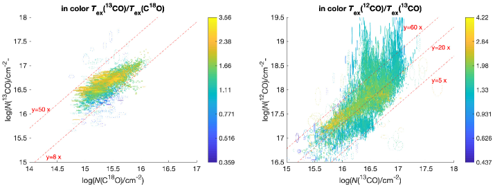
Maps of the CO isotopologue column density ratios are shown in Fig. 17 and scatter plots are displayed in Fig. 19. With no isotopic fractionation and all carbon locked in CO, the expected CO isotopologue ratios are ¹²CO/¹³CO $=57-67$ and ¹³CO/C¹⁸O $=7.5-9.8$ using the elemental abundances given in the previous subsection. As shown in Fig. 19, the lower bound of the ratio of the ¹³CO and C¹⁸O column densities is indeed in the expected range at $N(^{13}$CO$)/N($C¹⁸O$)=8$. The upper bound is close to 50 indicating that chemical effects play a significant role, by enhancing the ¹³CO abundance (fractionation) and/or destroying C¹⁸O (photodissociation).

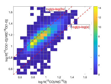
Figure 20 suggests that the column density ratio is well correlated with the ratio of line intensities, but the column density ratio is a factor up to 1.75 smaller than the ratio of line intensities because of the difference in excitation temperatures and of the moderate opacity of the ¹³CO(1-0) line. Ratios of integrated intensities can therefore be used to estimate the column density ratios, but after checking with radiative transfer calculations for a possible multiplicative bias and introducing a correction if needed.

Although the derivations of ¹²CO column densities are uncertain, the column density ratio $N(^{12}$CO$)/N(^{13}$CO$)$ ranges between 10 and 60. In particular, the low values of the ratio remain even when the opacity of the ¹²CO line becomes small enough to accurately derive the column density. Such low values are found in diffuse and translucent gas as a consequence of efficient fractionation in ¹³C due to the exchange reaction between ¹³C⁺ and ¹²CO, that enhances the ¹³CO abundance (Liszt & Pety, 2012). The physical conditions in the translucent envelope of Orion B seem to favor fractionation, which is not restricted to a small subset of the mapped area but it seen over wide areas. As discussed by Bron et al. (2018) the presence of chemical fractionation over the whole region can be identified by comparing the ratio of integrated intensities of the CO isotopologues, and looking at the data in the W(${}^{13}\mathrm{CO}$)/W(${}^{12}\mathrm{CO}$) versus W(${}^{13}\mathrm{CO}$)/W($\mathrm{C}^{18}\mathrm{O}$) plane. The existence of this chemical fractionation implies that using a single value for the abundance ratios of CO isotopologues can introduce significant errors when attempting to correct for the CO opacity in computing its column densities as done by Barnes et al. (2018) for instance. This will further increase the bias introduced by using the same excitation temperature for ¹²CO and ¹³CO ground state transitions. In addition to possibly biasing the results, using such simplifying assumptions is also expected to increase the dispersion and affect the overall determination of the $X_{\mathrm{CO}}=N(\mathrm{H_{2}})/W(\mathrm{CO})$ conversion factor.

6.5 Velocity dispersions

Maps of the velocity dispersions for ¹³CO, C¹⁸O, and ¹²CO are shown in Fig. 13. The mean values are listed in Table 2 and the ratios for the different CO isotopologues are listed in Table 3. Our formalism includes the line broadening due to opacity (see, e.g., Phillips et al., 1979), which is very significant for ¹²CO. This implies that the actual velocity dispersion derived from high opacity lines like those of ¹²CO is smaller than the apparent line width. Because we fixed the ¹²CO velocity dispersion to the value obtained with ¹³CO in our estimation, the velocity dispersions of ¹²CO and ¹³CO are identical (see Sect. 5.2). The velocity dispersions of C¹⁸O and ¹³CO are however fitted independently. Both species show similar velocity dispersions but ¹³CO has consistently broader line profiles than C¹⁸O. The ratio between the velocity dispersions of ¹³CO and C¹⁸O is 1.1 (see Table 3). The ¹³CO emission is produced by a more extended volume along the line of sight than the C¹⁸O emission as shown by the lower threshold in N(H₂) where ¹³CO is detected as discussed above. When analyzing the filamentary structure of the Orion B molecular cloud, Orkisz et al. (2019) showed that the gas velocity dispersion determined from C¹⁸O reaches a minimum value in the filament ridges, and is always lower than the velocity dispersion determined by ¹³CO. The refined analysis presented here, which takes the opacity broadening effect into account, confirms the presence of gradients in velocity dispersion across the spatial extent of the cloud and along the line of sight, which are captured by the difference between ¹³CO and C¹⁸O. Inspecting the spatial distribution of the velocity in Fig. 13 suggests that the small excess of velocity dispersion for ¹³CO relative to C¹⁸O is more prominent in the regions with relatively low $T_{\mathrm{dust}}$. This supports the hypothesis that this variation of velocity dispersion is tracing the starting point of the dissipation of turbulence when entering the dense filamentary skeleton of the molecular cloud.

7 Conclusion

This paper presents an analysis of the precision of the estimation of physical parameters ($\Delta_{V},\sigma_{V},N,T_{\mathrm{ex}}$) when trying to fit spectra of low $J$ transitions for the most common CO isotopologues, using the LTE radiative transfer model. This analysis was based on the Cramer Rao bound (CRB) computation. We applied this analysis to the region of the Orion B molecular cloud that contains the Horsehead pillar and the NGC 2023 and IC 434 Hii regions with the following astrophysical results.

• The mean abundances of the CO isotopologues are consistent with previous determinations in other regions: $\mathrm{X(^{12}CO)}\sim 6\times 10^{-5}$, $\mathrm{X(^{13}CO)}=2.5\pm 1.5\times 10^{-6}$, and $\mathrm{X(C^{18}O)}=2.0\pm 0.8\times 10^{-7}$.

• The excitation temperatures $T_{\mathrm{ex}}$ are different among the CO isotopologues. ¹²CO presents the highest $T_{\mathrm{ex}}$, followed by ¹³CO and C¹⁸O. For ¹³CO and C¹⁸O, the excitation temperatures are lower than the dust temperature on average, while they are higher for ¹²CO. This systematic variation can be understood as resulting from gradients of physical conditions along the line of sight together with the increased effect of radiative trapping for the more abundant isotopologues.

• These differences in $T_{\mathrm{ex}}$ imply that the ratio of ${}^{13}\mathrm{CO}$(1$-$0) and $\mathrm{C}^{18}\mathrm{O}$(1$-$0) integrated intensities is not a direct measurement of the column density ratio $N{\rm{(^{13}CO)}}/N\rm{(C^{18}O)}$, with a difference of up to a factor two. Moreover, this column density ratio exhibits regular spatial variations across the mapped region, with high values in the UV illuminated regions and low values in shielded regions. These low values are consistent with the ratio of ¹³C and ¹⁸O elemental abundances (i.e., a factor of about 8).

• In this nearby molecular cloud, the elemental abundances are uniform and the variations in CO isotopologue relative abundances are solely due to chemical processes (fractionation, photodissociation, freezing). The interpretation of variations of line integrated intensity ratios should therefore be performed with caution, taking into account radiative transfer and chemical effects.

We obtained the following results from the methodological viewpoint.

• This analysis has shown that it is important to take the opacity broadening effect into account when fitting the line profiles, even for moderate opacities as first discussed by Phillips et al. (1979). The estimation of the column density is correlated with that of the velocity dispersion when the line is optically thick and this correlation between column density and velocity dispersion must be taken into account when estimating uncertainties on the fitted parameters even for moderate line opacities. When the line is optically thin, the estimation of the column density is correlated with that of the excitation temperature except in a small interval where the ratio of the column density of the species to the integrated intensity of the line reaches a minimum (around $T_{\rm{ex}}=10$ K for the 1-0 transitions of CO isotopologues). This means that a small variation of the estimation of the excitation temperature or velocity dispersion will lead to large errors on the estimation of the column density.

• This analysis also allows us to quantify the benefit of a simultaneous analysis of two rotational lines of the same species compared to the analysis of a single line. In particular, it alleviates the degeneracy described above. This is a rigorous demonstration of intuitive results. It is an argument in favor of the installation of dual-band receiver systems for telescopes like the IRAM-30m or NOEMA.

• In order to derive the precision achieved on these parameters when trying to fit actual observations of the CO isotopologue lines towards the Orion B molecular cloud, we first showed that a (simple) maximum likelihood estimator is unbiased and efficient when the relative precision given by the CRB is better than $20\%$, and that it is possible to detect pixels for which the estimation of the parameters in LTE conditions is accurate (i.e., better than $20\%$).

• The residuals of the fit of the CO isotopologue lines amount to less than 1% of the original signal and the relative precision on the physical parameters is better than 20% for 63%, 82%, and 40% of the field of view for the ¹²CO, ¹³CO, and C¹⁸O species, respectively. The presence of structured residuals nevertheless indicates that the model remains sometimes too simple. In particular, asymmetric line profiles or the presence of line wings are incorrectly modeled. The ¹²CO line profiles are the most affected. Addressing the possibility of catching the complex shape of this spectrum is a motivating perspective that would generalize the approach initiated in this paper.

In the transition between regions where the number of required velocity components changes, some ambiguity on the velocities of the components occurs, and this impacts the estimations of all the other parameters. Fixing a priori $\Delta_{V}$ based on spatial processing (e.g. extending the ROHSA pre-processing) and thus applying only a gradient on $\sigma_{V}$, $T_{\mathrm{ex}}$ and $N$ could improve the robustness of our estimations. This would be useful, in particular, for low signal-to-noise ratio pixels. Another perspective is to use a spatial regularization criterion in the fit to improve all the estimations. This will be the subject of another paper (Vono et al., in prep.). Finally, trying to estimate the above physical parameters in regions that are more diffuse than on the studied field of view or for other species that have higher dipole moments (HCO⁺ or CS), requires the use of non-LTE models. Such non-LTE models would also be interesting to identify possible systematic effects coming from the use of the LTE approximation. Another paper will study the Large Velocity Gradient approximation of the radiative transfer using a similar CRB approach.

Appendix A Gradient calculation

The spectrum at frequency $\nu$ is

$$s(\nu)=\left(J(T_{\mathrm{ex}},\nu_{l})-J(T_{\mathrm{CMB}},\nu)\right)\left[1-\exp(-\Psi(\nu))\right]$$ (32)

It it thus a function of the unknown parameters $\boldsymbol{\theta}=[T_{\mathrm{ex}},\,\log N,\,\Delta_{V},\,\sigma_{V}]$. The following gradients are useful to derive the Fisher matrix (see Eq. 14).

A.1 $\partial s(\nu)/\partial T_{\mathrm{ex}}$

$$\begin{array}[]{ll}\frac{\partial s(\nu)}{\partial T_{\mathrm{ex}}}=&\frac{\partial J(T_{\mathrm{ex}},\nu_{l})}{\partial T_{\mathrm{ex}}}\left[1-\exp(-\Psi(\nu))\right]\\ &+\left(J(T_{\mathrm{ex}},\nu_{l})-J(T_{\mathrm{CMB}},\nu)\right)\frac{\partial\Psi(\nu)}{\partial T_{\mathrm{ex}}}\exp(-\Psi(\nu))\end{array}$$ (33)

A.2 $\frac{\partial J(T,\nu)}{\partial T}$

$$J(T,\nu)=\frac{h\nu}{k}\frac{1}{\exp{\frac{h\nu}{kT}}-1}$$ (34)

Thus

$$\frac{\partial J(T,\nu)}{\partial T}=\frac{h\nu}{k}\frac{\frac{h\nu}{kT^{2}}\exp{\frac{h\nu}{kT}}}{\left(\exp{\frac{h\nu}{kT}}-1\right)^{2}}=\frac{h^{2}\nu^{2}}{k^{2}T^{2}}\frac{\exp{\frac{h\nu}{kT}}}{\left(\exp{\frac{h\nu}{kT}}-1\right)^{2}}$$ (35)

and finally

$$\frac{\partial J(T,\nu)}{\partial T}=\frac{h^{2}\nu^{2}}{k^{2}T^{2}}\frac{1}{\exp{\frac{h\nu}{kT}}-2+\exp{-\frac{h\nu}{kT}}}$$ (36)

A.3 $\frac{\partial\Psi(\nu)}{\partial T_{\mathrm{ex}}}$

$$\Psi(\nu)=\sum_{l=1}^{2}\alpha_{l}\phi\left(\nu;\nu_{l}\left(1-\frac{\Delta_{V}}{c}\right),\nu_{l}\frac{\sigma_{V}}{c}\right)$$ (37)

Thus

$$\frac{\partial\Psi(\nu)}{\partial T_{\mathrm{ex}}}=\sum_{l=1}^{2}\frac{\partial\alpha_{l}}{\partial T_{\mathrm{ex}}}\phi\left(\nu;\nu_{l}\left(1-\frac{\Delta_{V}}{c}\right),\nu_{l}\frac{\sigma_{V}}{c}\right)$$ (38)

A.4 $\frac{\partial\alpha_{l}}{\partial T_{\mathrm{ex}}}$

$$\alpha_{l}=\frac{c^{2}}{8\pi}\frac{N}{Q(T_{\mathrm{ex}})}\frac{A_{l}\,g_{\mathrm{up}}}{\nu_{l}^{2}}\exp\left[-\frac{E_{\mathrm{up}}}{T_{\mathrm{ex}}}\right]\left(\exp\left[\frac{h\,\nu_{l}}{k\,T_{\mathrm{ex}}}\right]-1\right)$$ (39)

Thus,

$$\frac{\partial\alpha_{l}}{\partial T_{\mathrm{ex}}}=\left(-\frac{Q^{\prime}(T_{\mathrm{ex}})}{Q(T_{\mathrm{ex}})}+\frac{E_{\mathrm{up}}}{T_{\mathrm{ex}}^{2}}-\frac{h\,\nu_{l}}{k\,T_{\mathrm{ex}}^{2}}\frac{1}{1-\exp-\frac{h\,\nu_{l}}{k\,T_{\mathrm{ex}}}}\right)\alpha_{l}$$ (40)

where $Q^{\prime}(T_{\mathrm{ex}})=\frac{\partial Q(T_{\mathrm{ex}})}{\partial T_{\mathrm{ex}}}$ is numerically computed.

A.5 $\partial s(\nu)/\partial L_{N}$

Let us introduce $L_{N}=\log N$.

$$\frac{\partial s(\nu)}{\partial L_{N}}=\left(J(T_{\mathrm{ex}},\nu_{l})-J(T_{\mathrm{CMB}},\nu)\right)\frac{\partial\Psi(\nu)}{\partial L_{N}}\exp(-\Psi(\nu))$$ (41)

A.6 $\frac{\partial\alpha_{l}}{\partial L_{N}}$

Since $N=10^{L_{N}}$ and using Eq. (39), one gets

$$\frac{\partial\alpha_{l}}{\partial L_{N}}=\alpha_{l}\ln(10)$$ (42)

where $\ln$ is the natural logarithm.

A.7 $\partial\Psi(\nu)/\partial L_{N}$

From Eq. (37), one gets

$$\frac{\partial\Psi(\nu)}{\partial L_{N}}=\sum_{l=1}^{L}\frac{\partial\alpha_{l}}{\partial L_{N}}\phi\left(\nu;\nu_{l}\left(1-\frac{\Delta_{V}}{c}\right),\nu_{l}\frac{\sigma_{V}}{c}\right)$$ (43)

Then using Eq. (42), one gets

$$\frac{\partial\Psi(\nu)}{\partial L_{N}}=\log(10)\,\Psi(\nu)$$ (44)

A.8 $\partial s(\nu)/\partial\Delta_{V}$

$$\frac{\partial s(\nu)}{\partial\Delta_{V}}=\left(J(T_{\mathrm{ex}},\nu_{l})-J(T_{\mathrm{CMB}},\nu)\right)\frac{\partial\Psi(\nu)}{\partial\Delta_{V}}\exp(-\Psi(\nu))$$ (45)

A.9 $\partial\Psi(\nu)/\partial\Delta_{V}$

With $\nu_{c}=\nu_{l}\left(1-\frac{\Delta_{V}}{c}\right)$ and $\sigma_{\nu}=\nu_{l}\frac{\sigma_{V}}{c}$ one has

$$\Psi(\nu)=\sum_{l=1}^{2}\alpha_{l}\,\phi\left(\nu;\nu_{c},\sigma_{\nu}\right)$$ (46)

Thus

$$\frac{\partial\Psi(\nu)}{\partial\Delta_{V}}=\sum_{l=1}^{2}\alpha_{l}\frac{\partial\phi\left(\nu;\nu_{c},\sigma_{\nu}\right)}{\partial\Delta_{V}}$$ (47)

Since $\phi(\nu;\nu_{c},\sigma_{\nu})=\frac{1}{\sqrt{2\pi}\sigma_{\nu}}\exp\left(-\frac{(\nu-\nu_{c})^{2}}{2\sigma_{\nu}^{2}}\right)$, one gets

$$\frac{\partial\Psi(\nu)}{\partial\Delta_{V}}=-\sum_{l=1}^{2}\alpha_{l}\frac{\nu_{l}}{c}\frac{\partial\phi(\nu;\nu_{c},\sigma_{\nu})}{\partial\nu_{c}}$$ (48)

where

$$\frac{\partial\phi(\nu;\nu_{c},\sigma_{\nu})}{\partial\nu_{c}}=\frac{2(\nu-\nu_{c})}{2\sigma_{\nu}^{2}}\phi(\nu;\nu_{c},\sigma_{\nu})$$ (49)

Thus

$$\frac{\partial\Psi(\nu)}{\partial\Delta_{V}}=-\sum_{l=1}^{2}\alpha_{l}\frac{\nu_{l}}{c}\frac{(\nu-\nu_{c})}{\sigma_{\nu}^{2}}\phi\left(\nu;\nu_{c},\sigma_{\nu}\right)$$ (50)

A.10 $\partial s(\nu)/\partial\sigma_{V}$

$$\frac{\partial s(\nu)}{\partial\sigma_{V}}=\left(J(T_{\mathrm{ex}},\nu_{l})-J(T_{\mathrm{CMB}},\nu)\right)\frac{\partial\Psi(\nu)}{\partial\sigma_{V}}\exp(-\Psi(\nu))$$ (51)

A.11 $\partial\Psi(\nu)/\partial\sigma_{V}$

From Eq. (46), one gets

$$\frac{\partial\Psi(\nu)}{\partial\sigma_{V}}=\sum_{l=1}^{2}\alpha_{l}\,\frac{\partial\phi\left(\nu;\nu_{c},\sigma_{\nu}\right)}{\partial\sigma_{V}}$$ (52)

and with $\phi(\nu;\nu_{c},\sigma_{\nu})=\frac{1}{\sqrt{2\pi}\sigma_{\nu}}\exp\left(-\frac{(\nu-\nu_{c})^{2}}{2\sigma_{\nu}^{2}}\right)$, one gets

$$\frac{\partial\Psi(\nu)}{\partial\sigma_{V}}=\sum_{l=1}^{2}\alpha_{l}\frac{\nu_{l}}{c}\frac{\partial\phi(\nu;\nu_{c},\sigma_{\nu})}{\partial\sigma_{\nu}}$$ (53)

Then,

$$\frac{\partial\phi(\nu;\nu_{c},\sigma_{\nu})}{\partial\sigma_{\nu}}=-\frac{1}{\sigma_{\nu}}\phi(\nu;\nu_{c},\sigma_{\nu})+\frac{2(\nu-\nu_{c})^{2}}{2\sigma_{\nu}^{3}}\phi(\nu;\nu_{c},\sigma_{\nu})$$ (54)

Thus

$$\frac{\partial\Psi(\nu)}{\partial\sigma_{V}}=\sum_{l=1}^{2}\alpha_{l}\frac{\nu_{l}}{c}\left(\frac{(\nu-\nu_{c})^{2}}{\sigma_{\nu}^{3}}-\frac{1}{\sigma_{\nu}}\right)\phi\left(\nu;\nu_{c},\sigma_{\nu}\right)$$ (55)

which can also be written

$$\frac{\partial\Psi(\nu)}{\partial\sigma_{V}}=\sum_{l=1}^{2}\alpha_{l}\frac{1}{\sigma_{V}}\left(\frac{(\nu-\nu_{c})^{2}}{\sigma_{\nu}^{2}}-1\right)\phi\left(\nu;\nu_{c},\sigma_{\nu}\right).$$ (56)

Appendix B Maximum Likelihood Estimator

B.1 Definition for two lines of the same species, and a single velocity component

We start with the assumption that we will estimate the physical parameters $(\boldsymbol{\theta})$ of the LTE radiative transfer for two lines of the same species, and a single velocity component. Starting from Eq. (13), we note the $2K$ samples $x_{n,l}$ as $\boldsymbol{\chi}$. The amount of noise for each line is fixed to $\sigma_{b,1}$, and $\sigma_{b,2}$. In this case, the maximum likelihood estimator (MLE) is (Garthwaite et al., 1995)

$$\widehat{}\boldsymbol{\theta}=\arg\max_{\boldsymbol{\theta}}\left(\log l(\boldsymbol{\theta};\boldsymbol{\chi})\right).$$ (57)

Thus, $\widehat{}\boldsymbol{\theta}$ is the argument that maximizes the likelihood for the observed sample $\boldsymbol{\chi}$. With two lines, the likelihood can be written as

$$l(\boldsymbol{\theta};\boldsymbol{\chi})=\prod_{l=1}^{2}\prod_{n=1}^{K}\frac{1}{\sqrt{2\pi}\sigma_{b,l}}\exp\left(-\frac{(x_{n,l}-s_{n,l})^{2}}{2\sigma_{b,l}^{2}}.\right)$$ (58)

And the log-likelihood is

$$L(\boldsymbol{\theta};\boldsymbol{\chi})=\mathrm{cte}-\sum_{l=1}^{2}\frac{\sum_{n=1}^{K}(x_{n,l}-s_{n,l})^{2}}{2\sigma_{b,l}^{2}}.$$ (59)

B.2 Initialization of the unknown parameters

The log-likelihood function $L(\boldsymbol{\theta};\boldsymbol{\chi})$ can have many local maxima. It is thus crucial to initialize the gradient near the global maximum. As explained in Sect. 4.1, the vector of unknown parameters has 4 components $(\boldsymbol{\theta}=[T_{\mathrm{ex}},\,\log N,\,\Delta_{V},\,\sigma_{V}]^{T})$ in the case of a single velocity component. A simple initial estimation of the typical velocity along the line of sight $(\Delta_{V})$ is given by the velocity where the spectrum intensity is maximum. As the three other unknown parameters ($T_{\mathrm{ex}}$, $N$, and $\sigma_{V}$) are highly correlated (see section 4.6), we systematically search in a 3D grid defined as follows.

• We sample $N$ logarithmically between $10^{12}$ and $10^{18}\mathrm{\,cm^{-2}}$ with a step of 0.1 (i.e., 61 values).

• We sample $T_{\mathrm{ex}}$ logarithmically between $3\mathrm{\,K}$ and $100\mathrm{\,K}$ with a step of 0.05 (i.e., 31 values).

• Finally, we first sample $\sigma_{V}$ with 0.2, 0.3, …, 0.6, 1.2,…, 3.8 km$/$s (i.e., 10 values) before refining the search with a step of $0.025\mathrm{\,km\,s^{-1}}$ for $\sigma_{V}\leq 0.6\mathrm{\,km\,s^{-1}}$, and of $0.05\mathrm{\,km\,s^{-1}}$ otherwise.

These values have been fixed empirically based on simulations for which we tried to find a tradeoff between accuracy and computation time.

B.3 Maximization of the likelihood function through a scoring algorithm

The likelihood function is maximized here using Fisher’s scoring algorithm (Garthwaite et al., 1995). It is an iterative algorithm

$$\widehat{}\boldsymbol{\theta}^{(i+1)}=\widehat{}\boldsymbol{\theta}^{(i)}+p_{i}\boldsymbol{I}_{F}^{-1}(\widehat{}\boldsymbol{\theta}^{(i)})\nabla_{\boldsymbol{\theta}}(\widehat{}\boldsymbol{\theta}^{(i)})$$ (60)

where $i$ is the ith iteration, $p_{i}$ is a constant, $\boldsymbol{I}_{F}(\boldsymbol{\theta})$ is the Fisher matrix (see Sect. 4) seen as a function of $\boldsymbol{\theta}$, and $\nabla_{\boldsymbol{\theta}}(\boldsymbol{\theta})$ is the gradient

$$\forall j=1,...,4\quad\left[\nabla_{\boldsymbol{\theta}}(\boldsymbol{\theta})\right]_{j}=\sum_{l=1}^{2}\frac{1}{\sigma_{b,l}^{2}}\sum_{n=1}^{K}\frac{\partial s_{n,l}}{\partial\theta_{j}}(x_{n,l}-s_{n,l}),$$ (61)

where $j$ is the index of the unknown parameter.

In practice, at each iteration $i$, the algorithm tries $p_{i}=0.1$, $0.4$ and $0.8$, and it makes a quadratic fit to get an estimation of $p_{i}$ that minimizes the log-likelihood in the interval $[0.1,\,0.8]$. Moreover, the inversion of $\boldsymbol{I}_{F}$ is made with the pseudo-inverse when $\boldsymbol{I}_{F}$ becomes singular (in the sense that the ratio between the largest and the smallest eigenvalues of $\boldsymbol{I}_{F}$ is larger than $10^{8}$). Finally, the iteration loop stops when the log-likelihood verifies $|L(\widehat{}\boldsymbol{\theta}^{(i+1)};\boldsymbol{\chi})-L(\widehat{}\boldsymbol{\theta}^{(i)};\boldsymbol{\chi})|<10^{-16}$ or when the number of iterations reaches 1000.

B.4 Generalization to two velocity components

When two velocity components are needed, the log-likelihood of Eq. (59) becomes

$$L(\boldsymbol{\theta}_{1},\boldsymbol{\theta}_{2};\boldsymbol{\chi})=\mathrm{cte}-\sum_{l=1}^{2}\frac{\sum_{n=1}^{K}(x_{n,l}-s_{n,l}(\boldsymbol{\theta}_{1})-s_{n,l}(\boldsymbol{\theta}_{2}))^{2}}{2\sigma_{b,l}^{2}}$$ (62)

where $s_{n,l}(\boldsymbol{\theta}_{m})$ is the spectrum corresponding to the component $m\in\{1,2\}$. The grid used in the initialization step has now six dimensions: $T_{\mathrm{ex}}^{(1)},N^{(1)},\sigma_{V}^{(1)},T_{\mathrm{ex}}^{(2)},N^{(2)},\sigma_{V}^{(2)}$. One solution is to consider the total Fisher matrix of size $8\times 8$ (see section 4.2), but it can lead to singularities. We empirically observe that using iteratively the gradient on each component separately ($\boldsymbol{\theta}_{1}$, and then $\boldsymbol{\theta}_{2}$) actually leads to better results than using a gradient on the enlarged vector $[\boldsymbol{\theta}_{1},\,\boldsymbol{\theta}_{2}]^{T}$. Such a coordinate descent only requires inversions of $4\times 4$ Fisher matrices.

B.5 Computing load and optimization

From the computational viewpoint, the estimation will be done many times either because it will be applied to many different lines of sight or because it will be used in Monte Carlo simulations. It is thus useful to actually compute in advance a 5D set of $\left(s_{n}(\boldsymbol{\theta})\right)_{n,T_{\mathrm{ex}},N,\sigma_{V},\Delta_{V}}$ per line. In this 5D set, $T_{\mathrm{ex}}$, $N$ and $\sigma_{V}$ are sampled as described in Sect. B.2. Moreover, we consider 10 different values of $\Delta_{V}$ with a step of $0.05\mathrm{\,km\,s^{-1}}$ and we restrict the range of explored channels to the velocity range where the lines appear, i.e., an interval of 26.5$\mathrm{\,km\,s^{-1}}$ around the initially estimated $\Delta_{V}$. This last point decreases substantially the computation time. For a single species, the computation of the 5D set of $\left(s_{n}(\boldsymbol{\theta})\right)_{n}$ takes around 13 seconds in our Matlab implementation on a standard 2016 laptop. Each subsequent estimation (initialization plus gradient) takes around 0.05 or 1.0 second when estimating one or two velocity components, respectively.

For the considered ORION-B data, and with the initialization proposed in Sect. B.2, the median number of iterations required to reach convergence is 40 or 200 when estimating one or two velocity components, respectively.

Appendix C Performance of the Maximum Likelihood Estimator

Figure 21: Variations of the relative number of accurate estimations as a function of the column density and excitation temperature. The contour corresponds to the frontier where the relative precision on the actual values of the four parameters is $\rho=20\%$ (solid red contour on the left), and $10\%$ (dashed red contour on the right). The ${}^{13}\mathrm{CO}$(1$-$0) and ${}^{13}\mathrm{CO}$(2$-$1) lines are simulated with $\sigma_{b}=100$$\mathrm{\,mK}$, $\Delta_{V}=1.1$$\mathrm{\,km\,s^{-1}}$, and $\sigma_{V}=0.61$$\mathrm{\,km\,s^{-1}}$.

Figure 22: Variations of the bias (left) and efficiency (right) of the maximum likelihood estimator as a function of the column density and excitation temperature. The solid and dashed red contours correspond to the frontiers where the relative precisions on the estimations on the four parameters are $\rho=20$, and $10\%$, respectively, as defined in Fig. 21. The ${}^{13}\mathrm{CO}$(1$-$0) and ${}^{13}\mathrm{CO}$(2$-$1) lines are simulated with $\sigma_{b}=100$$\mathrm{\,mK}$, $\Delta_{V}=1.1\mathrm{\,km\,s^{-1}}$, and $\sigma_{V}=0.61\mathrm{\,km\,s^{-1}}$.

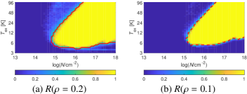
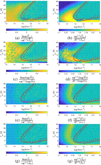
Monte Carlo simulations with $P$ independent realizations of the estimator $\left\{\widehat{}\boldsymbol{\theta}^{(p)}\right\}_{p=1,...,P}$ are used to analyze its performance. We simulate data for the ${}^{13}\mathrm{CO}$(1$-$0) and ${}^{13}\mathrm{CO}$(2$-$1) lines using the different values of $T_{\mathrm{ex}}$ and $N$ already used in Sect. 4.3. We here compute $P=200$ simulations with random noise for each pair of ($T_{\mathrm{ex}},N$) values.

After showing that MLE estimates of the parameters $(\widehat{}\boldsymbol{\theta})$ can be injected in the computation of the CRB to detect accurate estimations, we will show that the proposed estimator is unbiased and efficient.

C.1 Detection of (in)accurate estimations

In order to physically interpret the estimations $\widehat{}\boldsymbol{\theta}$ computed on observed data, it is crucial to remove inaccurate estimations. We thus need a way to quickly detect inaccurate estimations. Figure 21 shows the fraction of the Monte Carlo realizations for each pair of ($T_{\mathrm{ex}},N$) values that deliver “accurate” estimations of all parameters. “Accurate” here means that all the following conditions are simultaneously satisfied

$$\begin{array}[]{ll}{{\cal{B}}}^{1/2}(\widehat{T}_{\mathrm{ex}})/\widehat{T}_{\mathrm{ex}}\leq\rho,&{{\cal{B}}}^{1/2}(\log\widehat{N})\leq\rho,\\ {{\cal{B}}}^{1/2}(\widehat{\sigma}_{V})/\widehat{\sigma}_{V}\leq\rho,&{{\cal{B}}}^{1/2}(\widehat{\Delta}_{V})/\widehat{\sigma}_{V}\leq\rho.\end{array}$$ (63)

In these equations, $\rho$ is the relative precision required for all the parameters. At first sight, Eq. (63) and Eq. (25) seem identical. However, we here use estimation of the parameters $\widehat{}\boldsymbol{\theta}$, while we used values of $\boldsymbol{\theta}$ used to simulate the data in Sect. 4.7. The value $R(\rho)$ is the fraction of “accurate” estimations detected without a priori information on the parameters.

The contours in Fig. 21 correspond to the frontiers where the relative precision on the actual values $\boldsymbol{\theta}$ of the four parameters is $\rho=20\%$ or $10\%$. Figure 21 thus clearly suggests that these frontiers are close to the pixels for which $R(\rho)\simeq 0.5$. The test $R(\rho)\geq 0.5$ thus gives a fair detection of accurate (and inaccurate) estimations. Furthermore, these maps show that, most of the time, all $P$ estimations are either inaccurate ($R(\rho)=0$ in blue) or accurate ($R(\rho)=1$, in yellow). In other words, a single estimation $\widehat{}\boldsymbol{\theta}$ is often sufficient to detect whether it is accurate or not.

More precisely, the light blue area in Fig. 21.a corresponds to a value $R(0.2)=0.15$. This means that we still have a $15\%$ chance of considering an estimation as accurate when it is in fact inaccurate, when $N\simeq 10^{15}\mathrm{\,cm^{-2}}$ and $T_{\mathrm{ex}}>50\mathrm{\,K}$. It is possible to improve this on observed data because adjacent pixels on the sky have physical parameters that are partially correlated. We can thus assume that accurate and inaccurate estimations are spatially grouped, and the detection can be improved by computing Eq. (63) in a sliding window of size $3\times 3$ pixels. In practice, we remove estimations of pixels for which one of the neighbors in the $3\times 3$ pattern violates Eq. (63).

C.2 Bias and variance of the estimator

The bias and variance of the maximum likelihood estimator can be estimated with (Garthwaite et al., 1995)

$$\begin{array}[]{c}\widehat{\mathrm{bias}}(\widehat{\theta}_{i})=\frac{1}{P}\sum\widehat{\theta}^{(p)}_{i}-\theta_{i}\\ \widehat{\mathrm{var}}(\widehat{\theta}_{i})=\frac{1}{P-1}\sum\left(\theta^{(p)}_{i}-\frac{1}{P}\sum\widehat{\theta}^{(p)}_{i}\right)^{2},\end{array}$$ (64)

where $P$ is the number of simulations in the Monte Carlo analysis, $\theta_{i}$ are the actual values of the parameters, and $\widehat{\theta}_{i}$ are the estimated values. Figure 22 shows the variations of the ratios $\widehat{\mathrm{bias}}(\widehat{\theta}_{i})/\widehat{\mathrm{var}}^{1/2}(\widehat{\theta}_{i})$ and $\widehat{\mathrm{var}}^{1/2}(\widehat{\theta}_{i})/{\cal B}^{1/2}(\theta)$ as a function of $T_{\mathrm{ex}}$ and $N$.

It shows that the bias of the proposed estimator is negligible compared to its standard deviation (i.e., $\widehat{\mathrm{bias}}(\widehat{\theta}_{i})\ll\widehat{\mathrm{var}}^{1/2}(\widehat{\theta}_{i})$), and that its variance reaches the Cramer Rao bound (i.e., $\widehat{\mathrm{var}}(\widehat{\theta}_{i})\simeq{\cal{B}}(\theta_{i})$) in the region where the CRBs are sufficiently small to get accurate estimations.

Appendix D Additional figures

In section 5.5, Figure 12 shows the residuals for only one line. Figure 23 is a generalization to the other lines.

Figure 23: Spatial variations of the observed spectrum “energy” (first column), of the residual “energy” (second column), of their ratio (third column), and of the ratio of “energy” that has not been modeled. The unit of the color look-up table is Kelvin² or % depending on the column. White contours show the regions where two components have been detected.