NAT: Noise-Aware Training for Robust Neural Sequence Labeling

Abstract

Sequence labeling systems should perform reliably not only under ideal conditions but also with corrupted inputs—as these systems often process user-generated text or follow an error-prone upstream component. To this end, we formulate the noisy sequence labeling problem, where the input may undergo an unknown noising process and propose two Noise-Aware Training (NAT) objectives that improve robustness of sequence labeling performed on perturbed input: Our data augmentation method trains a neural model using a mixture of clean and noisy samples, whereas our stability training algorithm encourages the model to create a noise-invariant latent representation. We employ a vanilla noise model at training time. For evaluation, we use both the original data and its variants perturbed with real OCR errors and misspellings. Extensive experiments on English and German named entity recognition benchmarks confirmed that NAT consistently improved robustness of popular sequence labeling models, preserving accuracy on the original input. We make our code and data publicly available for the research community.

1 Introduction

Sequence labeling systems are generally trained on clean text, although in real-world scenarios, they often follow an error-prone upstream component, such as Optical Character Recognition (OCR; Neudecker, 2016) or Automatic Speech Recognition (ASR; Parada et al., 2011). Sequence labeling is also often performed on user-generated text, which may contain spelling mistakes or typos (Derczynski et al., 2013). Errors introduced in an upstream task are propagated downstream, diminishing the performance of the end-to-end system (Alex and Burns, 2014). While humans can easily cope with typos, misspellings, and the complete omission of letters when reading (Rawlinson, 2007), most Natural Language Processing (NLP) systems fail when processing corrupted or noisy text (Belinkov and Bisk, 2018). Although this problem is not new to NLP, only a few works addressed it explicitly (Piktus et al., 2019; Karpukhin et al., 2019). Other methods must rely on the noise that occurs naturally in the training data.

Figure 1: An example of a labeling error on a slightly perturbed sentence. Our noise-aware methods correctly predicted the location (LOC) label for the first word, as opposed to the standard approach, which misclassified it as an organization (ORG). We complement the example with a high-level idea of our noise-aware training, where the original sentence and its noisy variant are passed together through the system. The final loss is computed based on both sets of features, which improves robustness to the input perturbations.

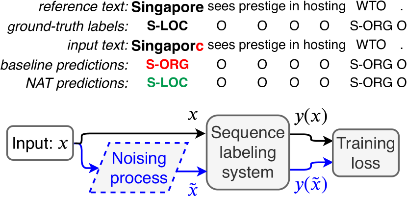
In this work, we are concerned with the performance difference of sequence labeling performed on clean and noisy input. Is it possible to narrow the gap between these two domains and design an approach that is transferable to different noise distributions at test time? Inspired by recent research in computer vision (Zheng et al., 2016), Neural Machine Translation (NMT; Cheng et al., 2018), and ASR (Sperber et al., 2017), we propose two Noise-Aware Training (NAT) objectives that improve the accuracy of sequence labeling performed on noisy input without reducing efficiency on the original data. Figure 1 illustrates the problem and our approach.

Our contributions are as follows:

• We formulate a noisy sequence labeling problem, where the input undergoes an unknown noising process (§2.2), and we introduce a model to estimate the real error distribution (§3.1). Moreover, we simulate real noisy input with a novel noise induction procedure (§3.2).

• We propose a data augmentation algorithm (§3.3) that directly induces noise in the input data to perform training of the neural model using a mixture of noisy and clean samples.

• We implement a stability training method (Zheng et al., 2016), adapted to the sequence labeling scenario, which explicitly addresses the noisy input data problem by encouraging the model to produce a noise-invariant latent representation (§3.4).

• We evaluate our methods on real OCR errors and misspellings against state-of-the-art baseline models (Peters et al., 2018; Akbik et al., 2018; Devlin et al., 2019) and demonstrate the effectiveness of our approach (§4).

• To support future research in this area and to make our experiments reproducible, we make our code and data publicly available.

2 Problem Definition

2.1 Neural Sequence Labeling

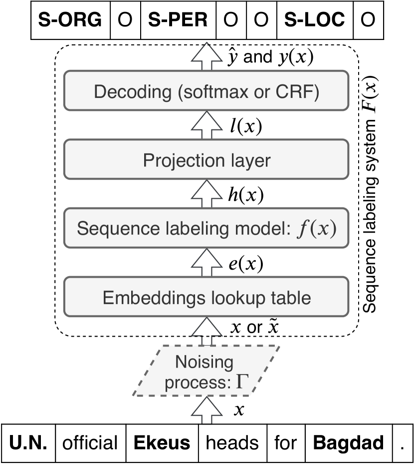
Figure 2 presents a typical architecture for the neural sequence labeling problem. We will refer to the sequence labeling system as $F(x;\theta)$, abbreviated as $F(x)$, where $x{\mkern 3.0mu{=}\mkern 3.0mu}(x_{1},\ldots,x_{N})$ is a tokenized input sentence of length $N$, and $\theta$ represents all learnable parameters of the system. $F(x)$ takes $x$ as input and outputs the probability distribution over the class labels $y(x)$ as well as the final sequence of labels $\hat{y}{\mkern 3.0mu{=}\mkern 3.0mu}(\hat{y}_{1},\ldots,\hat{y}_{N})$.

Either a softmax model (Chiu and Nichols, 2016) or a Conditional Random Field (CRF; Lample et al., 2016) can be used to model the output distribution over the class labels $y(x)$ from the logits $l(x)$, i.e., non-normalized predictions, and to output the final sequence of labels $\hat{y}$. As a labeled entity can span several consecutive tokens within a sentence, special tagging schemes are often employed for decoding, e.g., BIOES, where the Beginning, Inside, Outside, End-of-entity and Single-tag-entity sub-tags are also distinguished (Ratinov and Roth, 2009). This method introduces strong dependencies between subsequent labels, which are modeled explicitly by a CRF (Lafferty et al., 2001) that produces the most likely sequence of labels.

Figure 2: Neural sequence labeling architecture. In the standard scenario (§2.1), the original sentence $x$ is fed as input to the sequence labeling system $F(x)$. Token embeddings $e(x)$ are retrieved from the corresponding look-up table and fed to the sequence labeling model $f(x)$, which outputs latent feature vectors $h(x)$. The latent vectors are then projected to the class logits $l(x)$, which are used as input to the decoding model (softmax or CRF) that outputs the distribution over the class labels $y(x)$ and the final sequence of labels $\hat{y}$. In a real-world scenario (§2.2), the input sentence undergoes an unknown noising process $\Gamma$, and the perturbed sentence $\tilde{x}$ is fed to $F(x)$.

2.2 Noisy Neural Sequence Labeling

Similar to human readers, sequence labeling should perform reliably both in ideal and sub-optimal conditions. Unfortunately, this is rarely the case. User-generated text is a rich source of informal language containing misspellings, typos, or scrambled words (Derczynski et al., 2013). Noise can also be introduced in an upstream task, like OCR (Alex and Burns, 2014) or ASR (Chen et al., 2017), causing the errors to be propagated downstream.

To include the noise present on the source side of $F(x)$, we can modify its definition accordingly (Figure 2). Let us assume that the input sentence $x$ is additionally subjected to some unknown noising process $\Gamma{\mkern 3.0mu{=}\mkern 3.0mu}P(\tilde{x}_{i}{\mkern 1.0mu|\mkern 1.0mux_{i}})$, where $x_{i}$ is the original $i$-th token, and $\tilde{x}_{i}$ is its distorted equivalent. Let $\mathcal{V}$ be the vocabulary of tokens and $\tilde{\mathcal{V}}$ be a set of all finite character sequences over an alphabet $\Sigma$. $\Gamma$ is known as the noisy channel matrix (Brill and Moore, 2000) and can be constructed by estimating the probability $P(\tilde{x}_{i}{\mkern 1.0mu|\mkern 1.0mux_{i}})$ of each distorted token $\tilde{x}_{i}$ given the intended token $x_{i}$ for every $x_{i}\in\mathcal{V}$ and $\tilde{x}_{i}\in\tilde{\mathcal{V}}$.

2.3 Named Entity Recognition

We study the effectiveness of state-of-the-art Named Entity Recognition (NER) systems in handling imperfect input data. NER can be considered as a special case of the sequence labeling problem, where the goal is to locate all named entity mentions in unstructured text and to classify them into pre-defined categories, e.g., person names, organizations, and locations (Tjong Kim Sang and De Meulder, 2003). NER systems are often trained on the clean text. Consequently, they exhibit degraded performance in real-world scenarios where the transcriptions are produced by the previous upstream component, such as OCR or ASR (§2.2), which results in a detrimental mismatch between the training and the test conditions. Our goal is to improve the robustness of sequence labeling performed on data from noisy sources, without deteriorating performance on the original data. We assume that the source sequence of tokens $x$ may contain errors. However, the noising process is generally label-preserving, i.e., the level of noise is not significant enough to affect the corresponding labels. It follows that the noisy token $\tilde{x}_{i}$ inherits the ground-truth label $y_{i}$ from the underlying original token $x_{i}$.

3 Noise-Aware Training

3.1 Noise Model

To model the noise, we use the character-level noisy channel matrix $\Gamma$, which we will refer to as the character confusion matrix (§2.2).

Natural noise

We can estimate the natural error distribution by calculating the alignments between the pairs $(\tilde{x},x)\in\mathcal{P}$ of noisy and clean sentences using the Levenshtein distance metric (Levenshtein, 1966), where $\mathcal{P}$ is a corpus of paired noisy and manually corrected sentences (§2.2). The allowed edit operations include insertions, deletions, and substitutions of characters. We can model insertions and deletions by introducing an additional symbol $\varepsilon$ into the character confusion matrix. The probability of insertion and deletion can then be formulated as $P_{ins}(c{\mkern 1.0mu|\mkern 1.0mu\varepsilon})$ and $P_{del}(\varepsilon{\mkern 1.0mu|\mkern 1.0muc})$, where $c$ is a character to be inserted or deleted, respectively.

Synthetic noise

$\mathcal{P}$ is usually laborious to obtain. Moreover, the exact modeling of noise might be impractical, and it is often difficult to accurately estimate the exact noise distribution to be encountered at test time. Such distributions may depend on, e.g., the OCR engine used to digitize the documents. Therefore, we keep the estimated natural error distribution for evaluation and use a simplified synthetic error model for training. We assume that all types of edit operations are equally likely:

$$\smashoperator[lr]{\sum_{\tilde{c}\,\in\,\Sigma{\setminus}\{\varepsilon\}}^{}}P_{ins}(\tilde{c}{\mkern 1.0mu|\mkern 1.0mu\varepsilon})=P_{del}(\varepsilon{\mkern 1.0mu|\mkern 1.0muc})=\smashoperator[lr]{\sum_{\tilde{c}\,\in\,\Sigma{\setminus}\{c,\,\varepsilon\}}^{}}P_{subst}(\tilde{c}{\mkern 1.0mu|\mkern 1.0muc}),$$

where $c$ and $\tilde{c}$ are the original and the perturbed characters, respectively. Moreover, $P_{ins}$ and $P_{subst}$ are uniform over the set of allowed insertion and substitution candidates, respectively. We use the hyper-parameter $\eta$ to control the amount of noise to be induced with this method.

3.2 Noise Induction

Ideally, we would use the noisy sentences annotated with named entity labels for training our sequence labeling models. Unfortunately, such data is scarce. On the other hand, labeled clean text corpora are widely available (Tjong Kim Sang and De Meulder, 2003; Benikova et al., 2014). Hence, we propose to use the standard NER corpora and to induce noise into the input tokens during training synthetically.

In contrast to the image domain, which is continuous, the text domain is discrete, and we cannot directly apply continuous perturbations for written language. Although some works applied distortions at the level of embeddings (Miyato et al., 2017; Yasunaga et al., 2018; Bekoulis et al., 2018), we do not have a good intuition how it changes the meaning of the underlying textual input. Instead, we apply our noise induction procedure to generate distorted copies of the input. For every input sentence $x$, we independently perturb each token $x_{i}{\mkern 3.0mu{=}\mkern 3.0mu}(c_{1},\ldots,c_{K})$, where $K$ is the length of $x_{i}$, with the following procedure (Figure 3):

1. We insert the $\varepsilon$ symbol before the first and after every character of $x_{i}$ to get an extended token $x_{i}^{\prime}{\mkern 3.0mu{=}\mkern 3.0mu}(\varepsilon,c_{1},\varepsilon,\ldots,\varepsilon,c_{K},\varepsilon)$.

2. For every character $c^{\prime}_{k}$ of $x^{\prime}_{i}$, we sample the replacement character $\tilde{c}_{k}^{\prime}$ from the corresponding probability distribution $P(\tilde{c}_{k}^{\prime}{\mkern 1.0mu|\mkern 1.0muc_{k}^{\prime}})$, which can be obtained by taking a row of the character confusion matrix that corresponds to $c^{\prime}_{k}$. As a result, we get a noisy version of the extended input token $\tilde{x}_{i}^{\prime}$.

3. We remove all $\varepsilon$ symbols from $\tilde{x}^{\prime}_{i}$ and collapse the remaining characters to obtain a noisy token $\tilde{x}_{i}$.

Figure 3: Illustration of our noise induction procedure. Three examples correspond to insertion, deletion, and substitution errors. $x_{i}$, $x_{i}^{\prime}$, $\tilde{x}_{i}^{\prime}$, and $\tilde{x}_{i}$ are the original, extended, extended noisy, and noisy tokens, respectively.

3.3 Data Augmentation Method

We can improve robustness to noise at test time by introducing various forms of artificial noise during training. We distinct regularization methods like dropout (Srivastava et al., 2014) and task-specific data augmentation that transforms the data to resemble noisy input. The latter technique was successfully applied in other domains, including computer vision (Krizhevsky et al., 2012) and speech recognition (Sperber et al., 2017).

During training, we artificially induce noise into the original sentences using the algorithm described in §3.2 and train our models using a mixture of clean and noisy sentences. Let $\mathcal{L}_{0}(x,y;\theta)$ be the standard training objective for the sequence labeling problem, where $x$ is the input sentence, $y$ is the corresponding ground-truth sequence of labels, and $\theta$ represents the parameters of $F(x)$. We define our composite loss function as follows:

$$\begin{split}\mathcal{L}_{augm}(x,\tilde{x},y;\theta)&{\mkern 3.0mu{=}\mkern 3.0mu}\mathcal{L}_{0}(x,y;\theta)+\alpha\mathcal{L}_{0}(\tilde{x},y;\theta),\end{split}$$

where $\tilde{x}$ is the perturbed sentence, and $\alpha$ is a weight of the noisy loss component. $\mathcal{L}_{augm}$ is a weighted sum of standard losses calculated using clean and noisy sentences. Intuitively, the model that would optimize $\mathcal{L}_{augm}$ should be more robust to imperfect input data, retaining the ability to perform well on clean input. Figure 4(a) presents a schematic visualization of our data augmentation approach.

3.4 Stability Training Method

Zheng et al. (2016) pointed out the output instability issues of deep neural networks. They proposed a training method to stabilize deep networks against small input perturbations and applied it to the tasks of near-duplicate image detection, similar-image ranking, and image classification. Inspired by their idea, we adapt the stability training method to the natural language scenario.

Our goal is to stabilize the outputs $y(x)$ of a sequence labeling system against small input perturbations, which can be thought of as flattening $y(x)$ in a close neighborhood of any input sentence $x$. When a perturbed copy $\tilde{x}$ is close to $x$, then $y(\tilde{x})$ should also be close to $y(x)$. Given the standard training objective $\mathcal{L}_{0}(x,y;\theta)$, the original input sentence $x$, its perturbed copy $\tilde{x}$ and the sequence of ground-truth labels $y$, we can define the stability training objective $\mathcal{L}_{stabil}$ as follows:

$$\begin{split}\mathcal{L}_{stabil}(x,\tilde{x},y;\theta)&{\mkern 3.0mu{=}\mkern 3.0mu}\mathcal{L}_{0}(x,y;\theta)+\alpha\mathcal{L}_{sim}(x,\tilde{x};\theta),\\ \mathcal{L}_{sim}(x,\tilde{x};\theta)&{\mkern 3.0mu{=}\mkern 3.0mu}\mathcal{D}\big{(}y(x),y(\tilde{x})\big{)},\end{split}$$

where $\mathcal{L}_{sim}$ encourages the similarity of the model outputs for both $x$ and $\tilde{x}$, $\mathcal{D}$ is a task-specific feature distance measure, and $\alpha$ balances the strength of the similarity objective. Let $R(x)$ and $Q(\tilde{x})$ be the discrete probability distributions obtained by calculating the softmax function over the logits $l(x)$ for $x$ and $\tilde{x}$, respectively:

$$\begin{split}R(x)&{\mkern 3.0mu{=}\mkern 3.0mu}P(y{\mkern 1.0mu|\mkern 1.0mux}){\mkern 3.0mu{=}\mkern 3.0mu}softmax\big{(}l(x)\big{)},\\ Q(\tilde{x})&{\mkern 3.0mu{=}\mkern 3.0mu}P(y{\mkern 1.0mu|\mkern 1.0mu\tilde{x}}){\mkern 3.0mu{=}\mkern 3.0mu}softmax\big{(}l(\tilde{x})\big{)}.\end{split}$$

We model $\mathcal{D}$ as Kullback–Leibler divergence ($\mathcal{D}_{KL}$), which measures the correspondence between the likelihood of the original and the perturbed input:

$$\begin{split}\mathcal{L}_{sim}(x,\tilde{x};\theta)&{\mkern 3.0mu{=}\mkern 3.0mu}\sum\nolimits_{i}\mathcal{D}_{KL}\big{(}R(x_{i}){\mkern 1.0mu\mathbin{\|}\mkern 1.0muQ(\tilde{x}_{i})}\big{)},\\ \mathcal{D}_{KL}\big{(}R(x){\mkern 1.0mu\mathbin{\|}\mkern 1.0muQ(\tilde{x})}\big{)}&{\mkern 3.0mu{=}\mkern 3.0mu}\sum\nolimits_{j}P(y_{j}{\mkern 1.0mu|\mkern 1.0mux})\log\frac{P(y_{j}{\mkern 1.0mu|\mkern 1.0mux})}{P(y_{j}{\mkern 1.0mu|\mkern 1.0mu\tilde{x}})},\end{split}$$

where $i$, $j$ are the token, and the class label indices, respectively. Figure 4(b) summarizes the main idea of our stability training method.

(a) Data augmentation training objective $\mathcal{L}_{augm}$.

(b) Stability training objective $\mathcal{L}_{stabil}$.

Figure 4: Schema of our auxiliary training objectives. $x$, $\tilde{x}$ are the original and the perturbed inputs, respectively, that are fed to the sequence labeling system $F(x)$. $\Gamma$ represents a noising process. $y(x)$ and $y(\tilde{x})$ are the output distributions over the entity classes for $x$ and $\tilde{x}$, respectively. $\mathcal{L}_{0}$ is the standard training objective. $\mathcal{L}_{augm}$ combines $\mathcal{L}_{0}$ computed on both outputs from $F(x)$. $\mathcal{L}_{stabil}$ fuses $\mathcal{L}_{0}$ calculated on the original input with the similarity objective $\mathcal{L}_{sim}$.

A critical difference between the data augmentation and the stability training method is that the latter does not use noisy samples for the original task, but only for the stability objective. Furthermore, both methods need perturbed copies of the input samples, which results in longer training time but could be ameliorated by fine-tuning the existing model for a few epochs.

4 Evaluation

4.1 Experiment Setup

Model architecture

We used a BiLSTM-CRF architecture (Huang et al., 2015) with a single Bidirectional Long-Short Term Memory (BiLSTM) layer and $256$ hidden units in both directions for $f(x)$ in all experiments. We considered four different text representations $e(x)$, which were used to achieve state-of-the-art results on the studied data set and should also be able to handle misspelled text and out-of-vocabulary (OOV) tokens:

• FLAIR (Akbik et al., 2018) learns a Bidirectional Language Model (BiLM) using an LSTM network to represent any sequence of characters. We used settings recommended by the authors and combined FLAIR with GloVe (Pennington et al., 2014; FLAIR + GloVe) for English and Wikipedia FastText embeddings (Bojanowski et al., 2017; FLAIR + Wiki) for German.

• BERT (Devlin et al., 2019) employs a Transformer encoder to learn a BiLM from large unlabeled text corpora and sub-word units to represent textual tokens. We use the BERT_BASE model in our experiments.

• ELMo (Peters et al., 2018) utilizes a linear combination of hidden state vectors derived from a BiLSTM word language model trained on a large text corpus.

• Glove/Wiki + Char is a combination of pre-trained word embeddings (GloVe for English and Wikipedia FastText for German) and randomly initialized character embeddings (Lample et al., 2016).

Training

We trained the sequence labeling model $f(x)$ and the final CRF decoding layer on top of the pre-trained embedding vectors $e(x)$, which were fixed during training, except for the character embeddings (Figure 2). We used a mixture of the original data and its perturbed copies generated from the synthetic noise distribution (§3.1) with our noise induction procedure (§3.2). We kept most of the hyper-parameters consistent with Akbik et al. (2018). We trained our models for at most $100$ epochs and used early stopping based on the development set performance, measured as an average F1 score of clean and noisy samples. Furthermore, we used the development sets of each benchmark data set for validation only and not for training.

Performance measures

We measured the entity-level micro average F1 score on the test set to compare the results of different models. We evaluated on both the original and the perturbed data using various natural error distributions. We induced OCR errors based on the character confusion matrix $\Gamma$ (§3.2) that was gathered on a large document corpus (Namysl and Konya, 2019) using the Tesseract OCR engine (Smith, 2007). Moreover, we employed two sets of misspellings released by Belinkov and Bisk (2018) and Piktus et al. (2019). Following the authors, we replaced every original token with the corresponding misspelled variant, sampling uniformly among available replacement candidates. We present the estimated error rates of text that is produced with these noise induction procedures in Table 5 in the appendix. As the evaluation with noisy data leads to some variance in the final scores, we repeated all experiments five times and reported mean and standard deviation.

Implementation

We implemented our models using the FLAIR framework (Akbik et al., 2019). We extended their sequence labeling model by integrating our auxiliary training objectives (§3.3, §3.4). Nonetheless, our approach is universal and can be implemented in any other sequence labeling framework.

4.2 Sequence Labeling on Noisy Data

To validate our approach, we trained the baseline models with and without our auxiliary loss objectives (§3.3, §3.4). We used the CoNLL 2003 (Tjong Kim Sang and De Meulder, 2003) and the GermEval 2014 (Benikova et al., 2014) data sets in this setup. The baselines utilized GloVe vectors coupled with FLAIR and character embeddings (FLAIR + GloVe, GloVe + Char), BERT, and ELMo embeddings for English. For German, we employed Wikipedia FastText vectors paired with FLAIR and character embeddings (FLAIR + Wiki, Wiki + Char). We used a label-preserving training setup ($\alpha{\mkern 3.0mu{=}\mkern 3.0mu}1.0$, $\eta_{train}{\mkern 3.0mu{=}\mkern 3.0mu}10\%$).

Data set	Model	Train loss	Original data	OCR errors	Misspellings†	Misspellings‡
English CoNLL 2003	FLAIR + GloVe	$\mathcal{L}_{0}$	92.05	76.44$\pm$0.45	75.09$\pm$0.48	87.57$\pm$0.10
		$\mathcal{L}_{augm}$	92.56 (+0.51)	84.79$\pm$0.23 (+8.35)	83.57$\pm$0.43 (+8.48)	90.50$\pm$0.08 (+2.93)
		$\mathcal{L}_{stabil}$	91.99 (-0.06)	84.39$\pm$0.37 (+7.95)	82.43$\pm$0.23 (+7.34)	90.19$\pm$0.14 (+2.62)
	BERT	$\mathcal{L}_{0}$	90.91	68.23$\pm$0.39	65.65$\pm$0.31	85.07$\pm$0.15
		$\mathcal{L}_{augm}$	90.84 (-0.07)	79.34$\pm$0.32 (+11.11)	75.44$\pm$0.28 (+9.79)	86.21$\pm$0.24 (+1.14)
		$\mathcal{L}_{stabil}$	90.95 (+0.04)	78.22$\pm$0.17 (+9.99)	73.46$\pm$0.34 (+7.81)	86.52$\pm$0.12 (+1.45)
	ELMo	$\mathcal{L}_{0}$	92.16	72.90$\pm$0.50	70.99$\pm$0.17	88.59$\pm$0.19
		$\mathcal{L}_{augm}$	91.85 (-0.31)	84.09$\pm$0.18 (+11.19)	82.33$\pm$0.40 (+11.34)	89.50$\pm$0.16 (+0.91)
		$\mathcal{L}_{stabil}$	91.78 (-0.38)	83.86$\pm$0.11 (+10.96)	81.47$\pm$0.29 (+10.48)	89.49$\pm$0.15 (+0.90)
	GloVe + Char	$\mathcal{L}_{0}$	90.26	71.15$\pm$0.51	70.91$\pm$0.39	87.14$\pm$0.07
		$\mathcal{L}_{augm}$	90.83 (+0.57)	81.09$\pm$0.47 (+9.94)	79.47$\pm$0.24 (+8.56)	88.82$\pm$0.06 (+1.68)
		$\mathcal{L}_{stabil}$	90.21 (-0.05)	80.33$\pm$0.29 (+9.18)	78.07$\pm$0.23 (+7.16)	88.47$\pm$0.13 (+1.33)
German CoNLL 2003	FLAIR + Wiki	$\mathcal{L}_{0}$	86.13	66.93$\pm$0.49	78.06$\pm$0.13	80.72$\pm$0.23
		$\mathcal{L}_{augm}$	86.46 (+0.33)	75.90$\pm$0.63 (+8.97)	83.23$\pm$0.14 (+5.17)	84.01$\pm$0.27 (+3.29)
		$\mathcal{L}_{stabil}$	86.33 (+0.20)	75.08$\pm$0.29 (+8.15)	82.60$\pm$0.21 (+4.54)	84.12$\pm$0.26 (+3.40)
	Wiki + Char	$\mathcal{L}_{0}$	82.20	59.15$\pm$0.76	75.27$\pm$0.31	71.45$\pm$0.15
		$\mathcal{L}_{augm}$	82.62 (+0.42)	67.67$\pm$0.75 (+8.52)	78.48$\pm$0.24 (+3.21)	79.14$\pm$0.31 (+7.69)
		$\mathcal{L}_{stabil}$	82.18 (-0.02)	67.72$\pm$0.63 (+8.57)	77.59$\pm$0.12 (+2.32)	79.33$\pm$0.39 (+7.88)
Germ-Eval 2014	FLAIR + Wiki	$\mathcal{L}_{0}$	85.05	58.64$\pm$0.51	67.96$\pm$0.23	68.64$\pm$0.28
		$\mathcal{L}_{augm}$	84.84 (-0.21)	72.02$\pm$0.24 (+13.38)	78.59$\pm$0.11 (+10.63)	81.55$\pm$0.12 (+12.91)
		$\mathcal{L}_{stabil}$	84.43 (-0.62)	70.15$\pm$0.27 (+11.51)	75.67$\pm$0.16 (+7.71)	79.31$\pm$0.32 (+10.67)
	Wiki + Char	$\mathcal{L}_{0}$	80.32	52.48$\pm$0.31	61.99$\pm$0.35	54.86$\pm$0.15
		$\mathcal{L}_{augm}$	80.68 (+0.36)	63.74$\pm$0.31 (+11.26)	70.83$\pm$0.09 (+8.84)	75.66$\pm$0.11 (+20.80)
		$\mathcal{L}_{stabil}$	80.00 (-0.32)	62.29$\pm$0.35 (+9.81)	68.23$\pm$0.23 (+6.24)	72.40$\pm$0.29 (+17.54)

Table 1: Evaluation results on the CoNLL 2003 and the GermEval 2014 test sets. We report results on the original data, as well as on its noisy copies with OCR errors and two types of misspellings released by Belinkov and Bisk (2018)^† and Piktus et al. (2019)^‡. $\mathcal{L}_{0}$ is the standard training objective. $\mathcal{L}_{augm}$ and $\mathcal{L}_{stabil}$ are the data augmentation and the stability objectives, respectively. We report mean F1 scores with standard deviations from five experiments and mean differences against the standard objective (in parentheses).

Table 1 presents the results of this experiment. We found that our auxiliary training objectives boosted accuracy on noisy input data for all baseline models and both languages. At the same time, they preserved accuracy for the original input. The data augmentation objective seemed to perform slightly better than the stability objective. However, the chosen hyper-parameter values were rather arbitrary, as our goal was to prove the utility and the flexibility of both objectives.

4.3 Sensitivity Analysis

We evaluated the impact of our hyper-parameters on the sequence labeling accuracy using the English CoNLL 2003 data set. We trained multiple models with different amounts of noise $\eta_{train}$ and different weighting factors $\alpha$. We chose the FLAIR + GloVe model as our baseline because it achieved the best results in the preliminary analysis (§4.2) and showed good performance, which enabled us to perform extensive experiments.

(a) Data augmentation objective (original test data).

(b) Stability training objective (original test data).

(c) Data augmentation objective (tested on OCR errors)

(d) Stability training objective (tested on OCR errors)

Figure 5: Sensitivity analysis performed on the English CoNLL 2003 test set (§4.3). Each figure presents the results of models trained using one of our auxiliary training objectives on either original data or its variant perturbed with OCR errors. The bar marked as ”OCR” represents a model trained using the OCR noise distribution. Other bars correspond to models trained using synthetic noise distribution and different hyper-parameters ($\alpha$, $\eta_{train}$).

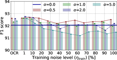
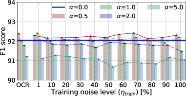
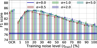
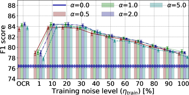
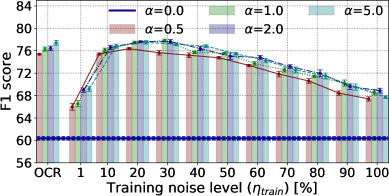
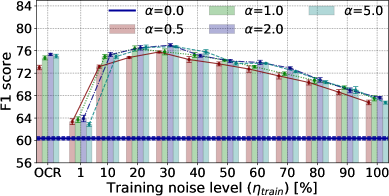
Figure 5 summarizes the results of the sensitivity experiment. The models trained with our auxiliary objectives mostly preserved or even improved accuracy on the original data compared to the baseline model ($\alpha{\mkern 3.0mu{=}\mkern 3.0mu}0$). Moreover, they significantly outperformed the baseline on data perturbed with natural noise. The best accuracy was achieved for $\eta_{train}$ from $10$ to $30\%$, which roughly corresponds to the label-preserving noise range. Similar to Heigold et al. (2018) and Cheng et al. (2019), we conclude that a non-zero noise level induced during training $({\eta_{train}>0})$ always yields improvements on noisy input data when compared with the models trained exclusively on clean data. The best choice of $\alpha$ was in the range from $0.5$ to $2.0$. $\alpha=5.0$ exhibited lower performance on the original data. Moreover, the models trained on the real error distribution demonstrated at most slightly better performance, which indicates that the exact noise distribution does not necessarily have to be known at training time.

4.4 Error Analysis

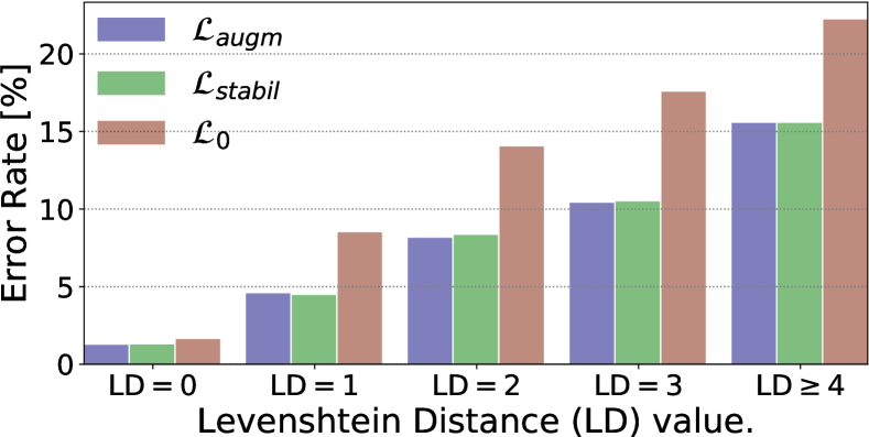
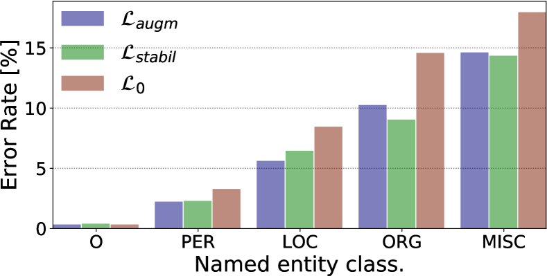
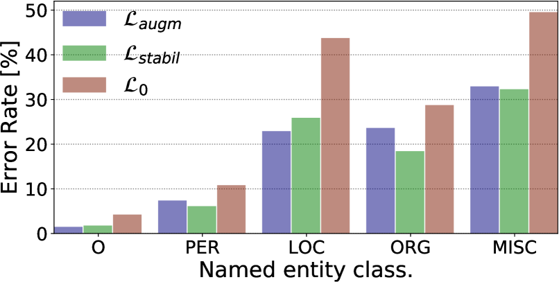
To quantify improvements provided by our approach, we measured sequence labeling accuracy on the subsets of data with different levels of perturbation, i.e., we divided input tokens based on edit distance to their clean counterparts. Moreover, we partitioned the data by named entity class to assess the impact of noise on recognition of different entity types. For this experiment, we used both the test and the development parts of the English CoNLL 2003 data set and induced OCR errors with our noising procedure.

Figure 6 presents the results for the baseline and the proposed methods. It can be seen that our approach achieved significant error reduction across all perturbation levels and all entity types. Moreover, by narrowing down the analysis to perturbed tokens, we discovered that the baseline model was particularly sensitive to noisy tokens from the LOC and the MISC categories. Our approach considerably reduced this negative effect. Furthermore, as the stability training worked slightly better on the LOC class and the data augmentation was more accurate on the ORG type, we argue that both methods could be combined to enhance overall sequence labeling accuracy further. Note that even if the particular token was not perturbed, its context could be noisy, which would explain the fact that our approach provided improvements even for tokens without perturbations.

(a) Divided by the edit distance value.

(b) Divided by the entity class (clean tokens).

(c) Divided by the entity class (perturbed tokens).

Figure 6: Error analysis results on the English CoNLL 2003 data set with OCR noise. We presented the results of the FLAIR + GloVe model trained with the standard and the proposed objectives. The data was divided into the subsets based on the edit distance of a token to its original counterpart and its named entity class. The latter group was further partitioned into the clean and the perturbed tokens. The error rate is the percentage of tokens with misrecognized entity class labels.

(Related Work)

5 Related Work

Improving robustness has been receiving increasing attention in the NLP community. The most relevant research was conducted in the NMT domain.

Noise-additive data augmentation

A natural strategy to improve robustness to noise is to augment the training data with samples perturbed using a similar noise model. Heigold et al. (2018) demonstrated that the noisy input substantially degrades the accuracy of models trained on clean data. They used word scrambling, as well as character flips and swaps as their noise model, and achieved the best results under matched training and test noise conditions. Belinkov and Bisk (2018) reported significant degradation in the performance of NMT systems on noisy input. They built a look-up table of possible lexical replacements from Wikipedia edit histories and used it as a natural source of the noise. Robustness to noise was only achieved by training with the same distribution—at the expense of performance degradation on other types of noise. In contrast, our method performed well on natural noise at test time by using a simplified synthetic noise model during training. Karpukhin et al. (2019) pointed out that existing NMT approaches are very sensitive to spelling mistakes and proposed to augment training samples with random character deletions, insertions, substitutions, and swaps. They showed improved robustness to natural noise, represented by frequent corrections in Wikipedia edit logs, without diminishing performance on the original data. However, not every word in the vocabulary has a corresponding misspelling. Therefore, even when noise is applied at the maximum rate, only a subset of tokens is perturbed (20-50%, depending on the language). In contrast, we used a confusion matrix, which is better suited to model statistical error distribution and can be applied to all tokens, not only those present in the corresponding look-up tables.

Robust representations

Another method to improve robustness is to design a representation that is less sensitive to noisy input. Zheng et al. (2016) presented a general method to stabilize model predictions against small input distortions. Cheng et al. (2018) continued their work and developed the adversarial stability training method for NMT by adding a discriminator term to the objective function. They combined data augmentation and stability objectives, while we evaluated both methods separately and provided evaluation results on natural noise distribution. Piktus et al. (2019) learned representation that embeds misspelled words close to their correct variants. Their Misspelling Oblivious Embeddings (MOE) model jointly optimizes two loss functions, each of which iterates over a separate data set (a corpus of text and a set of misspelling/correction pairs) during training. In contrast, our method does not depend on any additional resources and uses a simplified error distribution during training.

Adversarial learning

Adversarial attacks seek to mislead the neural models by feeding them with adversarial examples Szegedy et al. (2014). In a white-box attack scenario Goodfellow et al. (2015); Ebrahimi et al. (2018) we assume that the attacker has access to the model parameters, in contrast to the black-box scenario Alzantot et al. (2018); Gao et al. (2018), where the attacker can only sample model predictions on given examples. Adversarial training Miyato et al. (2017); Yasunaga et al. (2018), on the other hand, aims to improve the robustness of the neural models by utilizing adversarial examples during training.

The impact of noisy input data

In the context of ASR, Parada et al. (2011) observed that named entities are often OOV tokens, and therefore they cause more recognition errors. In the document processing field, Alex and Burns (2014) studied NER performed on several digitized historical text collections and showed that OCR errors have a significant impact on the accuracy of the downstream task. Namysl and Konya (2019) examined the efficiency of modern OCR engines and showed that although the OCR technology was more advanced than several years ago when many historical archives were digitized Kim and Cassidy (2015); Neudecker (2016), the most widely used engines still had difficulties with non-standard or lower quality input.

Spelling- and post-OCR correction.

A natural method of handling erroneous text is to correct it before feeding it to the downstream task. Most popular post-correction techniques include correction candidates ranking (Fivez et al., 2017; Flor et al., 2019), noisy channel modeling (Brill and Moore, 2000; Duan and Hsu, 2011), voting (Wemhoener et al., 2013), sequence to sequence models Afli et al. (2016); Schmaltz et al. (2017) and hybrid systems Schulz and Kuhn (2017).

In this paper, we have taken a different approach and attempted to make our models robust without relying on prior error correction, which, in case of OCR errors, is still far from being solved Chiron et al. (2017); Rigaud et al. (2019).

6 Conclusions

In this paper, we investigated the difference in accuracy between sequence labeling performed on clean and noisy text (§2.3). We formulated the noisy sequence labeling problem (§2.2) and introduced a model that can be used to estimate the real noise distribution (§3.1). We developed the noise induction procedure that simulates the real noisy input (§3.2). We proposed two noise-aware training methods that boost sequence labeling accuracy on the perturbed text: (i) Our data augmentation approach uses a mixture of clean and noisy examples during training to make the model resistant to erroneous input (§3.3). (ii) Our stability training algorithm encourages output similarity for the original and the perturbed input, which helps the model to build a noise invariant latent representation (§3.4). Our experiments confirmed that NAT consistently improved efficiency of popular sequence labeling models on data perturbed with different error distributions, preserving accuracy on the original input (§4). Moreover, we avoided expensive re-training of embeddings on noisy data sources by employing existing text representations. We conclude that NAT makes existing models applicable beyond the idealized scenarios. It may support an automatic correction method that uses recognized entity types to narrow the list of feasible correction candidates. Another application is data anonymization (Mamede et al., 2016).

Future work will involve improvements in the proposed noise model to study the importance of fidelity to real-world error patterns. Moreover, we plan to evaluate NAT on other real noise distributions (e.g., from ASR) and other sequence labeling tasks to support our claims further.

(Appendices)

Appendix A Noise Model - Supplementary Materials

In this section, we present the extended description of our vanilla noise model introduced in §3.1. Let $P_{edit}{\mkern 3.0mu{=}\mkern 3.0mu}\eta/{3}$ be the probability of performing a single character edit operation (insertion, deletion, or substitution) that replaces the source character $c$ with a noisy character $\tilde{c}$, where $\tilde{c}{\mkern 3.0mu{\neq}\mkern 3.0mu}{c}$. Equation 1 defines the vanilla error distribution, which we use at training time:

$$\frac{P_{edit}}{{\lvert\Sigma{\setminus}\{\varepsilon\}\rvert}}, \mkern 10.0mu\text{if}\ c{\mkern 3.0mu{=}\mkern 3.0mu}\varepsilon\ \text{and}\ \tilde{c}{\mkern 3.0mu{\neq}\mkern 3.0mu}{\varepsilon}.$$ (1a)

$$1-P_{edit}, \mkern 10.0mu\text{if}\ c{\mkern 3.0mu{=}\mkern 3.0mu}\varepsilon\ \text{and}\ \tilde{c}{\mkern 3.0mu{=}\mkern 3.0mu}{\varepsilon}.$$ (1b)

$$\frac{P_{edit}}{{\lvert\Sigma{\setminus}\{c,\varepsilon\}\rvert}}, \mkern 10.0mu\text{if}\ c{\mkern 3.0mu{\neq}\mkern 3.0mu}\varepsilon\ \text{and}\ \tilde{c}{\mkern 3.0mu{\neq}\mkern 3.0mu}{c}.$$ (1c)

$$P_{edit}, \mkern 10.0mu\text{if}\ c{\mkern 3.0mu{\neq}\mkern 3.0mu}\varepsilon\ \text{and}\ \tilde{c}{\mkern 3.0mu{=}\mkern 3.0mu}\varepsilon.$$ (1d)

$$1{-}2P_{edit}, \mkern 10.0mu\text{if}\ c{{\mkern 3.0mu{\neq}\mkern 3.0mu}}\varepsilon\ \text{and}\ \tilde{c}{\mkern 3.0mu{=}\mkern 3.0mu}{c}.$$ (1e)

It consists of the following components:

1. The insertion probability $P_{ins}(\tilde{c}{\mkern 1.0mu|\mkern 1.0mu\varepsilon})$ in eq. 1a. It describes how likely it is to insert a non-empty character $\tilde{c}{\mkern 3.0mu{\neq}\mkern 3.0mu}\varepsilon$ and it is uniform over the set of all characters from the alphabet $\Sigma$, except the $\varepsilon$ symbol.

2. The keep $\varepsilon$ probability $P_{keep}(\varepsilon{\mkern 1.0mu|\mkern 1.0mu\varepsilon})$ in eq. 1b.

3. The substitution probability $P_{subst}(\tilde{c}{\mkern 1.0mu|\mkern 1.0muc})$ in eq. 1c. It is uniform over the set of all characters from the alphabet $\Sigma$, except the source character $c$ and the $\varepsilon$ symbol.

4. The deletion probability $P_{del}(\varepsilon{\mkern 1.0mu|\mkern 1.0muc})$ in eq. 1d.

5. The keep probability $P_{keep}(c{\mkern 1.0mu|\mkern 1.0muc})$ in eq. 1e.

Equations 1a and 1b correspond to the row in the character confusion matrix $\Gamma$, where $c{\mkern 3.0mu{=}\mkern 3.0mu}\varepsilon$ and form a valid probability distribution:

$$P_{keep}(\varepsilon{\mkern 1.0mu|\mkern 1.0mu\varepsilon})+\smashoperator[lr]{\sum_{\tilde{c}\,\in\,\Sigma{\setminus}\{\varepsilon\}}^{}}P_{ins}(\tilde{c}{\mkern 1.0mu|\mkern 1.0muc}) =1.$$

Similarly, eqs. 1c, 1d and 1e correspond to the rows in the character confusion matrix $\Gamma$, where $c\in\Sigma{\setminus}\{\varepsilon\}$, and are also valid probability distributions:

$$P_{del}(\varepsilon{\mkern 1.0mu|\mkern 1.0muc})+P_{keep}(c{\mkern 1.0mu|\mkern 1.0muc})+\smashoperator[lr]{\sum_{\tilde{c}\,\in\,\Sigma{\setminus}\{c,\,\varepsilon\}}^{}}P_{subst}(\tilde{c}{\mkern 1.0mu|\mkern 1.0muc}) =1$$

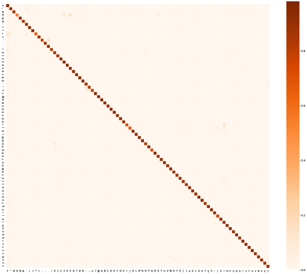
Finally, for comparison, we present visualizations of the confusion matrices used in our vanilla (Figure 7(a)) and OCR error models (Figure 7(b)).

(a) Vanilla error distribution used at training time ($\eta=20\%$).

(b) Real error distribution estimated from a large document corpus using the Tesseract OCR engine.

Figure 7: Confusion matrices for the vanilla and the OCR error distributions. Each cell represents $P(\tilde{c}{\mkern 1.0mu|\mkern 1.0muc})$. The rows correspond to the original characters $c$ and the columns represent the perturbed characters $\tilde{c}$. In this example, we include all symbols from the alphabet of the English CoNLL 2003 data set. The vanilla noise model assigns equal probability to all substitution errors, while the OCR error model is biased towards substitutions of characters with similar shapes like ”I”$\rightarrow$”l”, ”$”$\rightarrow$”5”, ”O”$\rightarrow$”0” or ”,”$\rightarrow$”.”. Moreover, the vanilla model assumes that the deletion of a character $c$ is as likely as the sum of substitution probabilities with all non-empty symbols: $P_{del}(\varepsilon{\mkern 1.0mu|\mkern 1.0muc}){\mkern 3.0mu{=}\mkern 3.0mu}\sum_{{\tilde{c}\,\in\,\Sigma{\setminus}\{\varepsilon\}}}P_{subst}(\tilde{c}{\mkern 1.0mu|\mkern 1.0muc})$.

A.1 Sensitivity Analysis

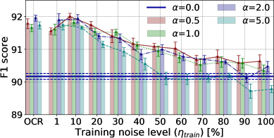
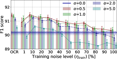
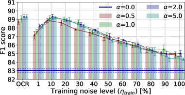
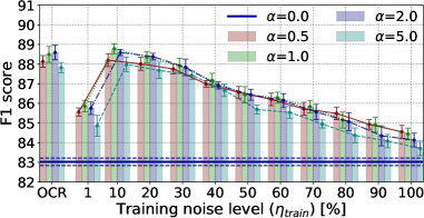
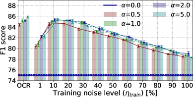
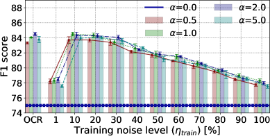
In this section, we present the extended version of our sensitivity study (§4.3). Figure 8 summarizes the results on the synthetic data distribution with various test- and training-time noise levels ($\eta_{test}$ and $\eta_{train}$, respectively) and weighting factors $\alpha$. We noticed a similar trend as in our initial analysis. As the level of noise $\eta_{test}$ increases, the overall accuracy decreases, but this trend is less pronounced for $\alpha\neq 0$. At the same time, the gap between the models trained with and without our auxiliary objectives becomes larger.

(a) Data augmentation objective (synthetic noise: $\eta_{test}{\mkern 3.0mu{=}\mkern 3.0mu}1\%$)

(b) Stability training (synthetic noise: $\eta_{test}{\mkern 3.0mu{=}\mkern 3.0mu}1\%$)

(c) Data augmentation objective (synthetic noise: $\eta_{test}{\mkern 3.0mu{=}\mkern 3.0mu}5\%$)

(d) Stability training objective(synthetic noise: $\eta_{test}{\mkern 3.0mu{=}\mkern 3.0mu}5\%$)

(e) Data augmentation objective (synthetic noise: $\eta_{test}{\mkern 3.0mu{=}\mkern 3.0mu}10\%$)

(f) Stability training objective (synthetic noise: $\eta_{test}{\mkern 3.0mu{=}\mkern 3.0mu}10\%$)

(g) Data augmentation objective (synthetic noise: $\eta_{test}{\mkern 3.0mu{=}\mkern 3.0mu}20\%$)

(h) Stability training objective (synthetic noise: $\eta_{test}{\mkern 3.0mu{=}\mkern 3.0mu}20\%$)

Figure 8: Extended results of our sensitivity analysis on the English CoNLL 2003 test data (§A.1). Each figure presents the results of models trained using one of our auxiliary training objectives on the original data perturbed with various levels of synthetic noise. The bar marked as ”OCR” represents a model trained using the OCR noise distribution. Other bars correspond to models trained using synthetic noise distribution and different hyper-parameters ($\alpha$, $\eta_{train}$).

A.2 Qualitative Analysis

In this section, we compared the outputs generated by the baseline models trained with and without our auxiliary training objectives (Table 2). We found that the NAT method improved robustness to capitalization errors (the first and the fourth row in Table 2(a)) as well as to substitutions (the second, the third and the fifth row in Table 2(a) and the first, the second, the fourth and the fifth row in Table 2(b)), deletions (the fifth row in Table 2(a)) and insertions of characters (the third and the fifth row in Table 2(b)). Moreover, it better recognized the semantics of the sentence in the third row of Table 2(a), where the location name was creatively rewritten (Brazland instead of Brazil).

1.	Reference result	7-1 Raul <B-PER> Gonzalez <E-PER> 7-1 Juan <B-PER> Pizzi <E-PER>
	NAT output	7-1 raul <B-PER> gonzalez <E-PER> 7-1 juan <B-PER> Pizzi <E-PER>
	Baseline output	7-1 raul gonzalez <S-PER> 7-1 juan Pizzi <S-PER>
2.	Reference result	6. Heidi <B-PER> Zurbriggen <E-PER> ( Switzerland <S-LOC> ) 153
	NAT output	6. Heidi <B-PER> Zurbriggen <E-PER> ( swizzerland <S-LOC> ) 153
	Baseline output	6. Heidi <B-PER> Zurbriggen <E-PER> ( swizzerland ) 153
3.	Reference result	Plastic surgery gets boost in Brazil <S-LOC> .
	NAT output	Plastic surgury hets boost is Brazland <S-LOC> .
	Baseline output	Plastic surgury hets boost is Brazland <S-PER> .
4.	Reference result	Waltraud <B-PER> Zimmer <E-PER> , Rödermark-Ober-Roden <S-LOC>
	NAT output	Waltraud <B-PER> zimmer <E-PER> , Rödermark-Ober-Roden <S-LOC>
	Baseline output	Waltraud <S-PER> zimmer , Rödermark-Ober-Roden <S-LOC>
5.	Reference result	Deutschland <S-LOC> ist noch nicht Teil der Reiseroute . "
	NAT output	Deutshland <S-LOC> is nach nich Teil der Reiseroute . "
	Baseline output	Deutshland <S-PER> is nach nich Teil der Reiseroute . "

(a) Misspellings.

1.	Reference result	Hapoel <B-ORG> Jerusalem <E-ORG> 12 4 1 7 10 18 13
	NAT output	Hapoel <B-ORG> lerusalem <E-ORG> I2 A 1 7 10 18 13
	Baseline output	Hapoel <S-ORG> lerusalem I2 A 1 7 10 18 13
2.	Reference result	SOCCER - SPANISH <S-MISC> FIRST DIVISION RESULT / STANDINGS .
	NAT output	SOCCER - SPANlSH <S-MISC> FIRST DIVISiOW RESULT / STA’DINGS .
	Baseline output	SOCCER - SPANlSH <S-PER> FIRST DIVISiOW RESULT / STA’DINGS .
3.	Reference result	EU <S-ORG> , Poland <S-LOC> agree on oil import tariffs .
	NAT output	EU <S-ORG> , Po’land <S-LOC> agree on oil import tarifs .
	Baseline output	EU <S-ORG> , Po’land <S-ORG> agree on oil import tarifs .
4.	Reference result	Schlamm scheint zu helfen - Yahoo <B-ORG> ! <E-ORG>
	NAT output	Schlamm scheint zu helfen - Yaho0 <B-ORG> ! <E-ORG>
	Baseline output	Schlamm scheint zu helfen - Yaho0 <S-PER> !
5.	Reference result	Fachverband <B-ORG> für <I-ORG> Hauswirtschaft <E-ORG> :
	NAT output	Fachverbandi <B-ORG> für <I-ORG> Hauswi’tschaTt <E-ORG> :
	Baseline output	Fachverbandi für Hauswi’tschaTt :

(b) OCR errors.

Table 2: Outputs produced by the models trained with and without our auxiliary NAT objectives (NAT output and Baseline output, respectively). We demonstrate examples that contain misspellings and OCR errors, where the models trained with the auxiliary NAT objectives correctly recognized all tags, while the baseline models either misclassified or completely missed some entities.

Appendix B Hyper-parameters

We present the detailed hyper-parameters of the sequence labeling model $f(x)$ used in our experiments (§4). Note that dropout was applied both before and after the LSTM layer (Table 3).

Parameter name	Parameter value
Tagging schema	BIOES
Mini batch size	32
Max. epochs	100
LSTM # hidden layers	1
LSTM # hidden units	256
Optimizer	SGD
Initial learning rate	0.1
Learning rate anneal factor	0.5
Minimum learning rate	0.0001
Word dropout level	0.05
Variational dropout level	0.5
Patience	3

Table 3: Hyper-parameters of the sequence labeling model $f(x)$ used in our experiments.

Appendix C Data Set Statistics and Estimated Error Rates

In this section, we present the detailed statistics of the data sets used in our NER experiments (Table 4). Following Akbik et al. (2018), we used the revisited version of German CoNLL 2003, which was prepared in 2006 and is believed to be more accurate, as the previous version was done by non-native speakers. Moreover, we used only the inner layer of annotation for GermEval 2014.

Finally, in Table 5, we report estimated error rates for all data sets and all noising procedures used in our experiments.

	Train	Dev	Test	Total
Sentences	14,041	3,250	3,453	20744
Tokens	203,621	51,362	46,435	301418
PER	6,600	1,842	1,617	10059
LOC	7,140	1,837	1,668	10645
ORG	6,321	1,341	1,661	9323
MISC	3,438	922	702	5062

(a) English CoNLL 2003.

	Train	Dev	Test	Total
Sentences	12,705	3,068	3,160	18933
Tokens	207,484	51,645	52,098	311227
PER	2,801	1,409	1,210	5420
LOC	4,273	1,216	1,051	6540
ORG	2,154	1,090	584	3828
MISC	780	216	206	1202

(b) German CoNLL 2003.

	Train	Dev	Test	Total
Sentences	24,000	2,200	5,100	31300
Tokens	452,853	41,653	96,499	591005
PER	7,679	711	1,639	10029
PER-deriv	62	2	11	75
PER-part	184	18	44	246
LOC	8,281	763	1,706	10750
LOC-deriv	2,808	235	561	3604
LOC-part	513	52	109	674
ORG	5,255	496	1,150	6901
ORG-deriv	41	3	8	52
ORG-part	805	91	172	1068
MISC	3,024	269	697	3990
MISC-deriv	236	16	39	291
MISC-part	190	18	42	250

(c) GermEval 2014.

Table 4: Statistics of the data sets used in our NER experiments (§4). We present statistics of the training (Train) development (Dev) and test (Test) sets, including the number of sentences, tokens, and entities: person names (PER), locations (LOC), organizations (ORG) and miscellaneous (MISC). The GermEval 2014 data set defines two additional fine-grained sub-labels: ”-part” and ”-deriv” that mark derivation and compound words, respectively, which stand in direct relation to Named Entities.

	OCR noise	Mis-spellings†	Mis-spellings‡
English CoNLL 2003	8.9%	16.5%	9.8%
German CoNLL 2003	9.0%	8.3%	8.0%
GermEval 2014	9.3%	8.6%	8.2%

(a) Character Error Rates.

	OCR noise	Mis-spellings†	Mis-spellings‡
English CoNLL 2003	35.6%	55.4%	48.3%
German CoNLL 2003	39.5%	26.5%	45.5%
GermEval 2014	41.2%	27.0%	47.9%

(b) Word Error Rates.

Table 5: Error rate estimation for different noise distributions. OCR noise is modeled with the character confusion matrix, whereas misspellings are induced using look-up tables released by Belinkov and Bisk (2018)^† and Piktus et al. (2019)^‡.

References

- Afli et al. (2016) Haithem Afli, Zhengwei Qiu, Andy Way, and Páraic Sheridan. 2016. Using SMT for OCR error correction of historical texts. In Proceedings of the Tenth International Conference on Language Resources and Evaluation (LREC 2016), pages 962–966, Portorož, Slovenia. European Language Resources Association (ELRA).
- Akbik et al. (2019) Alan Akbik, Tanja Bergmann, Duncan Blythe, Kashif Rasul, Stefan Schweter, and Roland Vollgraf. 2019. FLAIR: An easy-to-use framework for state-of-the-art NLP. In Proceedings of the 2019 Conference of the North American Chapter of the Association for Computational Linguistics (Demonstrations), pages 54–59, Minneapolis, Minnesota. Association for Computational Linguistics.
- Akbik et al. (2018) Alan Akbik, Duncan Blythe, and Roland Vollgraf. 2018. Contextual string embeddings for sequence labeling. In Proceedings of the 27th International Conference on Computational Linguistics, pages 1638–1649, Santa Fe, New Mexico, USA. Association for Computational Linguistics.
- Alex and Burns (2014) Beatrice Alex and John Burns. 2014. Estimating and rating the quality of optically character recognised text. In Proceedings of the First International Conference on Digital Access to Textual Cultural Heritage, DATeCH ’14, pages 97–102, New York, NY, USA. ACM.
- Alzantot et al. (2018) Moustafa Alzantot, Yash Sharma, Ahmed Elgohary, Bo-Jhang Ho, Mani Srivastava, and Kai-Wei Chang. 2018. Generating natural language adversarial examples. In Proceedings of the 2018 Conference on Empirical Methods in Natural Language Processing, pages 2890–2896, Brussels, Belgium. Association for Computational Linguistics.
- Bekoulis et al. (2018) Giannis Bekoulis, Johannes Deleu, Thomas Demeester, and Chris Develder. 2018. Adversarial training for multi-context joint entity and relation extraction. In Proceedings of the 2018 Conference on Empirical Methods in Natural Language Processing, pages 2830–2836, Brussels, Belgium. Association for Computational Linguistics.
- Belinkov and Bisk (2018) Yonatan Belinkov and Yonatan Bisk. 2018. Synthetic and natural noise both break neural machine translation. In 6th International Conference on Learning Representations, ICLR 2018, Vancouver, BC, Canada, April 30 - May 3, 2018, Conference Track Proceedings.
- Benikova et al. (2014) Darina Benikova, Chris Biemann, and Marc Reznicek. 2014. NoSta-d named entity annotation for German: Guidelines and dataset. In Proceedings of the Ninth International Conference on Language Resources and Evaluation (LREC-2014), pages 2524–2531, Reykjavik, Iceland. European Languages Resources Association (ELRA).
- Bojanowski et al. (2017) Piotr Bojanowski, Edouard Grave, Armand Joulin, and Tomas Mikolov. 2017. Enriching word vectors with subword information. Transactions of the Association for Computational Linguistics, 5:135–146.
- Brill and Moore (2000) Eric Brill and Robert C. Moore. 2000. An improved error model for noisy channel spelling correction. In Proceedings of the 38th Annual Meeting of the Association for Computational Linguistics, pages 286–293, Hong Kong. Association for Computational Linguistics.
- Chen et al. (2017) Pin-Jung Chen, I-Hung Hsu, Yi Yao Huang, and Hung-Yi Lee. 2017. Mitigating the impact of speech recognition errors on chatbot using sequence-to-sequence model. In 2017 IEEE Automatic Speech Recognition and Understanding Workshop, ASRU 2017, Okinawa, Japan, December 16-20, 2017, pages 497–503.
- Cheng et al. (2019) Yong Cheng, Lu Jiang, and Wolfgang Macherey. 2019. Robust neural machine translation with doubly adversarial inputs. In Proceedings of the 57th Annual Meeting of the Association for Computational Linguistics, pages 4324–4333, Florence, Italy. Association for Computational Linguistics.
- Cheng et al. (2018) Yong Cheng, Zhaopeng Tu, Fandong Meng, Junjie Zhai, and Yang Liu. 2018. Towards robust neural machine translation. In Proceedings of the 56th Annual Meeting of the Association for Computational Linguistics (Volume 1: Long Papers), pages 1756–1766, Melbourne, Australia. Association for Computational Linguistics.
- Chiron et al. (2017) G. Chiron, A. Doucet, M. Coustaty, and J. Moreux. 2017. ICDAR2017 competition on post-OCR text correction. In 2017 14th IAPR International Conference on Document Analysis and Recognition (ICDAR), volume 01, pages 1423–1428.
- Chiu and Nichols (2016) Jason P.C. Chiu and Eric Nichols. 2016. Named entity recognition with bidirectional LSTM-CNNs. Transactions of the Association for Computational Linguistics, 4:357–370.
- Derczynski et al. (2013) Leon Derczynski, Alan Ritter, Sam Clark, and Kalina Bontcheva. 2013. Twitter part-of-speech tagging for all: Overcoming sparse and noisy data. In Proceedings of the International Conference Recent Advances in Natural Language Processing RANLP 2013, pages 198–206, Hissar, Bulgaria. INCOMA Ltd. Shoumen, BULGARIA.
- Devlin et al. (2019) Jacob Devlin, Ming-Wei Chang, Kenton Lee, and Kristina Toutanova. 2019. BERT: Pre-training of deep bidirectional transformers for language understanding. In Proceedings of the 2019 Conference of the North American Chapter of the Association for Computational Linguistics: Human Language Technologies, Volume 1 (Long and Short Papers), pages 4171–4186, Minneapolis, Minnesota. Association for Computational Linguistics.
- Duan and Hsu (2011) Huizhong Duan and Bo-June (Paul) Hsu. 2011. Online spelling correction for query completion. WWW 2011.
- Ebrahimi et al. (2018) Javid Ebrahimi, Anyi Rao, Daniel Lowd, and Dejing Dou. 2018. HotFlip: White-box adversarial examples for text classification. In Proceedings of the 56th Annual Meeting of the Association for Computational Linguistics (Volume 2: Short Papers), pages 31–36, Melbourne, Australia. Association for Computational Linguistics.
- Fivez et al. (2017) Pieter Fivez, Simon Šuster, and Walter Daelemans. 2017. Unsupervised context-sensitive spelling correction of clinical free-text with word and character n-gram embeddings. In BioNLP 2017, pages 143–148, Vancouver, Canada,. Association for Computational Linguistics.
- Flor et al. (2019) Michael Flor, Michael Fried, and Alla Rozovskaya. 2019. A benchmark corpus of English misspellings and a minimally-supervised model for spelling correction. In Proceedings of the Fourteenth Workshop on Innovative Use of NLP for Building Educational Applications, pages 76–86, Florence, Italy. Association for Computational Linguistics.
- Gao et al. (2018) J. Gao, J. Lanchantin, M. L. Soffa, and Y. Qi. 2018. Black-box generation of adversarial text sequences to evade deep learning classifiers. In 2018 IEEE Security and Privacy Workshops (SPW), pages 50–56.
- Goodfellow et al. (2015) Ian Goodfellow, Jonathon Shlens, and Christian Szegedy. 2015. Explaining and harnessing adversarial examples. In International Conference on Learning Representations, ICLR 2015.
- Heigold et al. (2018) Georg Heigold, Stalin Varanasi, Günter Neumann, and Josef van Genabith. 2018. How robust are character-based word embeddings in tagging and MT against wrod scramlbing or randdm nouse? In Proceedings of the 13th Conference of the Association for Machine Translation in the Americas (Volume 1: Research Papers), pages 68–80, Boston, MA. Association for Machine Translation in the Americas.
- Huang et al. (2015) Zhiheng Huang, Wei Xu, and Kai Yu. 2015. Bidirectional LSTM-CRF models for sequence tagging. Computing Research Repository, arXiv:1508.01991.
- Karpukhin et al. (2019) Vladimir Karpukhin, Omer Levy, Jacob Eisenstein, and Marjan Ghazvininejad. 2019. Training on synthetic noise improves robustness to natural noise in machine translation. In Proceedings of the 5th Workshop on Noisy User-generated Text (W-NUT 2019), pages 42–47, Hong Kong, China. Association for Computational Linguistics.
- Kim and Cassidy (2015) Sunghwan Mac Kim and Steve Cassidy. 2015. Finding names in trove: Named entity recognition for Australian historical newspapers. In Proceedings of the Australasian Language Technology Association Workshop 2015, pages 57–65, Parramatta, Australia.
- Krizhevsky et al. (2012) Alex Krizhevsky, Ilya Sutskever, and Geoffrey E. Hinton. 2012. ImageNet classification with deep convolutional neural networks. In Proceedings of the 25th International Conference on Neural Information Processing Systems - Volume 1, NIPS’12, pages 1097–1105, USA. Curran Associates Inc.
- Lafferty et al. (2001) John D. Lafferty, Andrew McCallum, and Fernando C. N. Pereira. 2001. Conditional random fields: Probabilistic models for segmenting and labeling sequence data. In Proceedings of the Eighteenth International Conference on Machine Learning, ICML ’01, pages 282–289, San Francisco, CA, USA. Morgan Kaufmann Publishers Inc.
- Lample et al. (2016) Guillaume Lample, Miguel Ballesteros, Sandeep Subramanian, Kazuya Kawakami, and Chris Dyer. 2016. Neural architectures for named entity recognition. In Proceedings of the 2016 Conference of the North American Chapter of the Association for Computational Linguistics: Human Language Technologies, pages 260–270, San Diego, California. Association for Computational Linguistics.
- Levenshtein (1966) Vladimir Iosifovich Levenshtein. 1966. Binary codes capable of correcting deletions, insertions, and reversals. Soviet Physics-Doklady, 10(8).
- Mamede et al. (2016) Nuno Mamede, Jorge Baptista, and Francisco Dias. 2016. Automated anonymization of text documents. In 2016 IEEE Congress on Evolutionary Computation (CEC), pages 1287–1294. IEEE.
- Miyato et al. (2017) Takeru Miyato, Andrew M. Dai, and Ian J. Goodfellow. 2017. Adversarial training methods for semi-supervised text classification. In 5th International Conference on Learning Representations, ICLR 2017, Toulon, France, April 24-26, 2017, Conference Track Proceedings.
- Namysl and Konya (2019) Marcin Namysl and Iuliu Konya. 2019. Efficient, lexicon-free OCR using deep learning. In 2019 International Conference on Document Analysis and Recognition (ICDAR), pages 295–301.
- Neudecker (2016) Clemens Neudecker. 2016. An open corpus for named entity recognition in historic newspapers. In Proceedings of the Tenth International Conference on Language Resources and Evaluation (LREC 2016), pages 4348–4352, Portorož, Slovenia. European Language Resources Association (ELRA).
- Parada et al. (2011) Carolina Parada, Mark Dredze, and Frederick Jelinek. 2011. OOV sensitive named-entity recognition in speech. In INTERSPEECH 2011, 12th Annual Conference of the International Speech Communication Association, Florence, Italy, August 27-31, 2011, pages 2085–2088.
- Pennington et al. (2014) Jeffrey Pennington, Richard Socher, and Christopher Manning. 2014. Glove: Global vectors for word representation. In Proceedings of the 2014 Conference on Empirical Methods in Natural Language Processing (EMNLP), pages 1532–1543, Doha, Qatar. Association for Computational Linguistics.
- Peters et al. (2018) Matthew Peters, Mark Neumann, Mohit Iyyer, Matt Gardner, Christopher Clark, Kenton Lee, and Luke Zettlemoyer. 2018. Deep contextualized word representations. In Proceedings of the 2018 Conference of the North American Chapter of the Association for Computational Linguistics: Human Language Technologies, Volume 1 (Long Papers), pages 2227–2237, New Orleans, Louisiana. Association for Computational Linguistics.
- Piktus et al. (2019) Aleksandra Piktus, Necati Bora Edizel, Piotr Bojanowski, Edouard Grave, Rui Ferreira, and Fabrizio Silvestri. 2019. Misspelling oblivious word embeddings. In Proceedings of the 2019 Conference of the North American Chapter of the Association for Computational Linguistics: Human Language Technologies, Volume 1 (Long and Short Papers), pages 3226–3234, Minneapolis, Minnesota. Association for Computational Linguistics.
- Ratinov and Roth (2009) Lev Ratinov and Dan Roth. 2009. Design challenges and misconceptions in named entity recognition. In Proceedings of the Thirteenth Conference on Computational Natural Language Learning (CoNLL-2009), pages 147–155, Boulder, Colorado. Association for Computational Linguistics.
- Rawlinson (2007) Graham Rawlinson. 2007. The significance of letter position in word recognition. IEEE Aerospace and Electronic Systems Magazine, 22(1):26–27.
- Rigaud et al. (2019) C. Rigaud, A. Doucet, M. Coustaty, and J. Moreux. 2019. ICDAR 2019 competition on post-OCR text correction. In 2019 International Conference on Document Analysis and Recognition (ICDAR), pages 1588–1593.
- Schmaltz et al. (2017) Allen Schmaltz, Yoon Kim, Alexander Rush, and Stuart Shieber. 2017. Adapting sequence models for sentence correction. In Proceedings of the 2017 Conference on Empirical Methods in Natural Language Processing, pages 2807–2813, Copenhagen, Denmark. Association for Computational Linguistics.
- Schulz and Kuhn (2017) Sarah Schulz and Jonas Kuhn. 2017. Multi-modular domain-tailored OCR post-correction. In Proceedings of the 2017 Conference on Empirical Methods in Natural Language Processing, pages 2716–2726, Copenhagen, Denmark. Association for Computational Linguistics.
- Smith (2007) Ray Smith. 2007. An overview of the Tesseract OCR engine. In Proceedings of the Ninth International Conference on Document Analysis and Recognition (ICDAR 2007), volume 2, pages 629–633.
- Sperber et al. (2017) Matthias Sperber, Jan Niehues, and Alex Waibel. 2017. Toward robust neural machine translation for noisy input sequences. In The International Workshop on Spoken Language Translation (IWSLT), Tokyo, Japan.
- Srivastava et al. (2014) Nitish Srivastava, Geoffrey Hinton, Alex Krizhevsky, Ilya Sutskever, and Ruslan Salakhutdinov. 2014. Dropout: A simple way to prevent neural networks from overfitting. Journal of Machine Learning Research, 15:1929–1958.
- Szegedy et al. (2014) Christian Szegedy, Wojciech Zaremba, Ilya Sutskever, Joan Bruna, Dumitru Erhan, Ian Goodfellow, and Rob Fergus. 2014. Intriguing properties of neural networks. In International Conference on Learning Representations, ICLR 2014.
- Tjong Kim Sang and De Meulder (2003) Erik F. Tjong Kim Sang and Fien De Meulder. 2003. Introduction to the CoNLL-2003 shared task: Language-independent named entity recognition. In Proceedings of the Seventh Conference on Natural Language Learning at HLT-NAACL 2003, pages 142–147.
- Wemhoener et al. (2013) D. Wemhoener, I. Z. Yalniz, and R. Manmatha. 2013. Creating an improved version using noisy OCR from multiple editions. In 2013 12th International Conference on Document Analysis and Recognition, pages 160–164.
- Yasunaga et al. (2018) Michihiro Yasunaga, Jungo Kasai, and Dragomir Radev. 2018. Robust multilingual part-of-speech tagging via adversarial training. In Proceedings of the 2018 Conference of the North American Chapter of the Association for Computational Linguistics: Human Language Technologies, Volume 1 (Long Papers), pages 976–986, New Orleans, Louisiana. Association for Computational Linguistics.
- Zheng et al. (2016) Stephan Zheng, Yang Song, Thomas Leung, and Ian J. Goodfellow. 2016. Improving the robustness of deep neural networks via stability training. In 2016 IEEE Conference on Computer Vision and Pattern Recognition, CVPR 2016, Las Vegas, NV, USA, June 27-30, 2016, pages 4480–4488.