Smooth Exploration for Robotic Reinforcement Learning

Abstract

Reinforcement learning (RL) enables robots to learn skills from interactions with the real world. In practice, the unstructured step-based exploration used in Deep RL – often very successful in simulation – leads to jerky motion patterns on real robots. Consequences of the resulting shaky behavior are poor exploration, or even damage to the robot. We address these issues by adapting state-dependent exploration (SDE) [1] to current Deep RL algorithms. To enable this adaptation, we propose two extensions to the original SDE, using more general features and re-sampling the noise periodically, which leads to a new exploration method generalized state-dependent exploration (gSDE). We evaluate gSDE both in simulation, on PyBullet continuous control tasks, and directly on three different real robots: a tendon-driven elastic robot, a quadruped and an RC car. The noise sampling interval of gSDE permits to have a compromise between performance and smoothness, which allows training directly on the real robots without loss of performance. The code is available at https://github.com/DLR-RM/stable-baselines3.

1 Introduction

One of the first robots that used artificial intelligence methods was called “Shakey”, because it would shake a lot during operation [2]. Shaking has now again become quite prevalent in robotics, but for a different reason. When learning robotic skills with deep reinforcement learning (DeepRL), the de facto standard for exploration is to sample a noise vector $\epsilon_{t}$ from a Gaussian distribution independently at each time step $t$, and then adding it to the policy output. This approach leads to the type of noise illustrated to the left in Fig. 1, and it can be very effective in simulation [3, 4, 5, 6, 7].

Figure 1: Left: unstructured exploration, as typically used in simulated RL. Right: gSDE provides smooth and consistent exploration.

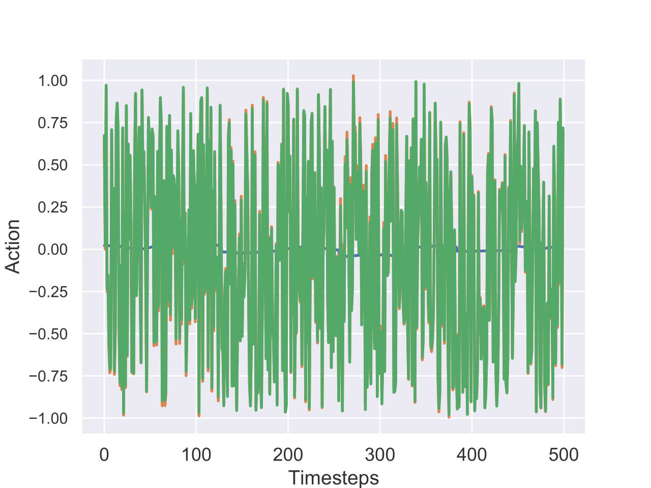
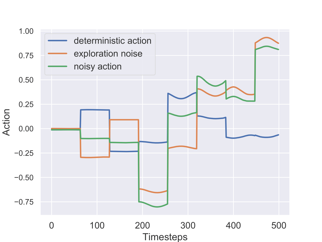
Unstructured exploration has also been applied to robotics [8, 9]. But for experiments on real robots, it has many drawbacks, which have been repeatedly pointed out [1, 10, 11, 12, 13]: 1) Sampling independently at each step leads to shaky behavior [14], and noisy, jittery trajectories. 2) The jerky motion patterns can damage the motors on a real robot, and lead to increased wear-and-tear. 3) In the real world, the system acts as a low pass filter. Thus, consecutive perturbations may cancel each other, leading to poor exploration. This is particularly true for high control frequency [15]. 4) It causes a large variance which grows with the number of time-steps [10, 11, 12]

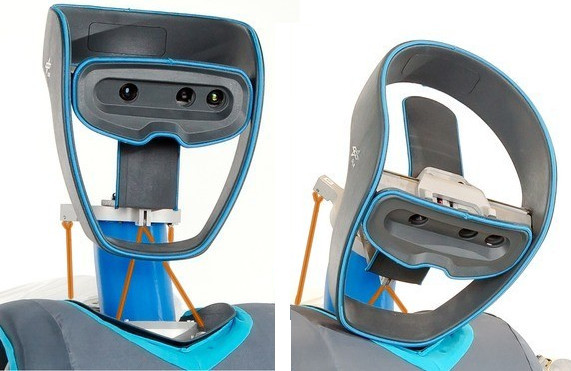
In practice, we have observed all of these drawbacks on three real robots, including the tendon-driven robot David, depicted in Fig. 4, which is the main experimental platform used in this work. For all practical purposes, Deep RL with unstructured noise cannot be applied to David.

In robotics, multiple solutions have been proposed to counteract the inefficiency of unstructured noise. These include correlated noise [8, 15], low-pass filters [16, 17], action repeat [18] or lower level controllers [16, 9]. A more principled solution is to perform exploration in parameter space, rather than in action space [19, 20]. This approach usually requires fundamental changes in the algorithm, and is harder to tune when the number of parameters is high.

State-Dependent Exploration (SDE) [1, 11] was proposed as a compromise between exploring in parameter and action space. SDE replaces the sampled noise with a state-dependent exploration function, which during an episode returns the same action for a given state. This results in smoother exploration and less variance per episode.

To the best of our knowledge, no Deep RL algorithm has yet been successfully combined with SDE. We surmise that this is because the problem that it solves – shaky, jerky movement – is not as noticeable in simulation, which is the current focus of the community.

In this paper, we aim at reviving interest in SDE as an effective method for addressing exploration issues that arise from using independently sampled Gaussian noise on real robots. Our concrete contributions, which also determine the structure of the paper, are:

1. Highlighting the issues with unstructured Gaussian exploration (Sect. 1).

2. Adapting SDE to recent Deep RL algorithms, and addressing some issues of the original formulation (Sects. 2.2 and 3).

3. Evaluate the different approaches with respect to the compromise between smoothness and performance, and show the impact of the noise sampling interval (Sects. 4.1 and 4.2).

4. Successfully applying RL directly on three real robots: a tendon-driven robot, a quadruped and an RC car, without the need of a simulator or filters (Sect. 4.3).

2 Background

In reinforcement learning, an agent interacts with its environment, usually modeled as a Markov Decision Process (MDP) $(\mathcal{S},\mathcal{A},p,r)$ where $\mathcal{S}$ is the state space, $\mathcal{A}$ the action space and $p(\mathbf{s}^{\prime}|\mathbf{s},\mathbf{a})$ the transition function. At every step $t$, the agent performs an action $\mathbf{a}$ in state $\mathbf{s}$ following its policy $\pi:\mathcal{S}\mapsto\mathcal{A}$. It then receives a feedback signal in the next state $\mathbf{s}^{\prime}$: the reward $r(\mathbf{s},\mathbf{a})$. The objective of the agent is to maximize the long-term reward. More formally, the goal is to maximize the expectation of the sum of discounted reward, over the trajectories $\rho_{\pi}$ generated using its policy $\pi$:

$$\sum_{t}\operatorname{\mathbb{E}}_{({\mathbf{s}_{t}},{\mathbf{a}_{t}})\sim\rho_{\pi}}\left[\gamma^{t}r({\mathbf{s}_{t}},{\mathbf{a}_{t}})\right]$$ (1)

where $\gamma\in[0,1)$ is the discount factor and represents a trade-off between maximizing short-term and long-term rewards. The agent-environment interactions are often broken down into sequences called episodes, that end when the agent reaches a terminal state.

2.1 Exploration in Action or Policy Parameter Space

In the case of continuous actions, the exploration is commonly done in the action space [21, 22, 23, 24, 25, 5]. At each time-step, a noise vector $\epsilon_{t}$ is independently sampled from a Gaussian distribution and then added to the controller output:

$${\mathbf{a}_{t}} =\mu({\mathbf{s}_{t}};\theta_{\mu})+\epsilon_{t}, \epsilon_{t}\sim\mathcal{N}(0,\sigma^{2})$$ (2)

where $\mu({\mathbf{s}_{t}})$ is the deterministic policy and $\pi({\mathbf{a}_{t}}|{\mathbf{s}_{t}})\sim\mathcal{N}(\mu({\mathbf{s}_{t}}),\sigma^{2})$ is the resulting stochastic policy, used for exploration. $\theta_{\mu}$ denotes the parameters of the deterministic policy.
For simplicity, throughout the paper, we will only consider Gaussian distributions with diagonal covariance matrices. Hence, here, $\sigma$ is a vector with the same dimension as the action space $\mathcal{A}$.

Alternatively, the exploration can also be done in the parameter space [11, 19, 20]:

$${\mathbf{a}_{t}} =\mu({\mathbf{s}_{t}};\theta_{\mu}+\epsilon), \epsilon\sim\mathcal{N}(0,\sigma^{2})$$ (3)

at the beginning of an episode, the perturbation $\epsilon$ is sampled and added to the policy parameters $\theta_{\mu}$. This usually results in more consistent exploration but becomes challenging with an increasing number of parameters [19].

2.2 State-Dependent Exploration

State-Dependent Exploration (SDE) [1, 11] is an intermediate solution that consists in adding noise as a function of the state ${\mathbf{s}_{t}}$, to the deterministic action $\mu({\mathbf{s}_{t}})$. At the beginning of an episode, the parameters $\theta_{\epsilon}$ of that exploration function are drawn from a Gaussian distribution. The resulting action ${\mathbf{a}_{t}}$ is as follows:

$${\mathbf{a}_{t}} =\mu({\mathbf{s}_{t}};\theta_{\mu})+\epsilon({\mathbf{s}_{t}};\theta_{\epsilon}), \theta_{\epsilon}\sim\mathcal{N}(0,\sigma^{2})$$ (4)

This episode-based exploration is smoother and more consistent than the unstructured step-based exploration. Thus, during one episode, instead of oscillating around a mean value, the action $\mathbf{a}$ for a given state $\mathbf{s}$ will be the same.

SDE should not be confused with unstructured noise where the variance can be state-dependent but the noise is still sampled at every step, as it is the case for SAC.

In the remainder of this paper, to avoid overloading notation, we drop the time subscript $t$, i. e. we now write $\mathbf{s}$ instead of ${\mathbf{s}_{t}}$. $\mathbf{s}_{j}$ or $\mathbf{a}_{j}$ now refer to an element of the state or action vector.

In the case of a linear exploration function $\epsilon(\mathbf{s};\theta_{\epsilon})=\theta_{\epsilon}\mathbf{s}$, by operation on Gaussian distributions, Rückstieß et al. [1] show that the action element $\mathbf{a}_{j}$ is normally distributed:

$$\pi_{j}(\mathbf{a}_{j}|\mathbf{s})\sim\mathcal{N}(\mu_{j}(\mathbf{s}),\hat{\sigma_{j}}^{2})$$ (5)

where $\hat{\sigma}$ is a diagonal matrix with elements $\hat{\sigma_{j}}=\sqrt{\sum_{i}{(\sigma_{ij}\mathbf{s}_{i})^{2}}}$.

Because we know the policy distribution, we can obtain the derivative of the log-likelihood $\log\pi(\mathbf{a}|\mathbf{s})$ with respect to the variance $\sigma$:

$$\frac{\partial\log\pi(\mathbf{a}|\mathbf{s})}{\partial\sigma_{ij}} =\frac{(\mathbf{a}_{j}-\mu_{j})^{2}-\hat{\sigma_{j}}^{2}}{\hat{\sigma_{j}}^{3}}\frac{\mathbf{s}_{i}^{2}\sigma_{ij}}{\hat{\sigma_{j}}}$$ (6)

This can be easily plugged into the likelihood ratio gradient estimator [26], which allows to adapt $\sigma$ during training. SDE is therefore compatible with standard policy gradient methods, while addressing most shortcomings of the unstructured exploration.

For a non-linear exploration function, the resulting distribution $\pi(\mathbf{a}|\mathbf{s})$ is most of the time unknown. Thus, computing the exact derivative w.r.t. the variance is not trivial and may require approximate inference. As we focus on simplicity, we leave this extension for future work.

3 Generalized State-Dependent Exploration

Considering Eqs. 5 and 7, some limitations of the original formulation are apparent:

1. The noise does not change during one episode, which is problematic if the episode length is long, because the exploration will be limited [27].

2. The variance of the policy $\hat{\sigma_{j}}=\sqrt{\sum_{i}{(\sigma_{ij}\mathbf{s}_{i})^{2}}}$ depends on the state space dimension (it grows with it), which means that the initial $\sigma$ must be tuned for each problem.

3. There is only a linear dependency between the state and the exploration noise, which limits the possibilities.

4. The state must be normalized, as the gradient and the noise magnitude depend on the state magnitude.

To mitigate the mentioned issues and adapt it to Deep RL algorithms, we propose two improvements:

1. We sample the parameters $\theta_{\epsilon}$ of the exploration function every $n$ steps instead of every episode.

2. Instead of the state $\mathbf{s}$, we can in fact use any features. We chose policy features $\mathbf{z_{\mu}}(\mathbf{s};\theta_{\mathbf{z_{\mu}}})$ (last layer before the deterministic output $\mu(\mathbf{s})=\theta_{\mu}\mathbf{z_{\mu}}(\mathbf{s};\theta_{\mathbf{z_{\mu}}})$) as input to the noise function $\epsilon(\mathbf{s};\theta_{\epsilon})=\theta_{\epsilon}\mathbf{z_{\mu}}(\mathbf{s})$.

Sampling the parameters $\theta_{\epsilon}$ every $n$ steps tackles the issue i. and yields a unifying framework [27] which encompasses both unstructured exploration ($n=1$) and original SDE ($n=\mathrm{episode\_length}$). Although this formulation follows the description of Deep RL algorithms that update their parameters every $m$ steps, the influence of this crucial parameter on smoothness and performance was until now overlooked.

Using policy features allows mitigating issues ii, iii and iv: the relationship between the state $\mathbf{s}$ and the noise $\epsilon$ is non-linear and the variance of the policy only depends on the network architecture, allowing for instance to use images as input. This formulation is therefore more general and includes the original SDE description, when using state as input to the noise function or when the policy is linear.

We call the resulting approach generalized State-Dependent Exploration (gSDE).

Deep RL algorithms

Integrating this updated version of SDE into recent Deep RL algorithms, such as those listed in the appendix, is straightforward. For those that rely on a probability distribution, such as SAC or PPO, we can replace the original Gaussian distribution by the one from Eq. 5, where the analytical form of the log-likelihood is known (cf. Eq. 7).

4 Experiments

In this section, we study gSDE to answer the following questions:

• How does gSDE compares to the original SDE? What is the impact of each proposed modification?

• How does gSDE compares to other type of exploration noise in terms of compromise between smoothness and performance?

• How does gSDE performs on a real system?

4.1 Compromise Between Smoothness and Performance

Experiment setup

In order to compare gSDE to other type of exploration in terms of compromise between performance and smoothness, we chose 4 locomotion tasks from the PyBullet [28] environments: HalfCheetah, Ant, Hopper and Walker2D. They are similar to the one found in OpenAI Gym [29] but the simulator is open source and they are harder to solve. In this section, we focus on the SAC algorithm as it will be the one used on the real robot, although we report results for additional algorithms such as PPO in the appendix.

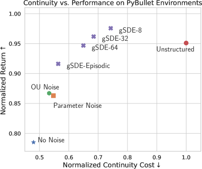
To evaluate smoothness, we define a continuity cost $\operatorname{\mathcal{C}}=100\times\operatorname{\mathbb{E}}_{t}\left[(\frac{\mathbf{a}_{t+1}-{\mathbf{a}_{t}}}{\Delta^{\mathbf{a}}_{\max}})^{2}\right]$ which yields values between 0 (constant output) and 100 (action jumping from one limit to another at every step). The continuity cost of the training $\operatorname{\mathcal{C}}_{\mathrm{train}}$ is a proxy for the wear-and-tear of the robot.

We compare the performance of the following configurations: (a) no exploration noise, (b) unstructured Gaussian noise (original SAC implementation), (c) correlated noise (Ornstein–Uhlenbeck process [30] with $\sigma{=}0.2$, OU noise in the figure), (d) adaptive parameter noise [19] ($\sigma{=}0.2$), (e) gSDE. To decorrelate the exploration noise from the one due to parameter update, and to be closer to a real robot setting, we apply the gradient updates only at the end of each episode.

We fix the budget to 1 million steps and report the average score over 10 runs together with the average continuity cost during training and their standard error. For each run, we test the learned policy on 20 evaluation episodes every 10000 steps, using the deterministic controller $\mu({\mathbf{s}_{t}})$. Regarding the implementation, we use a modified version of Stable-Baselines3 [31] together with the RL Zoo training framework [32]. The methodology we follow to tune the hyperparameters and their details can be found in the appendix. The code we used to run the experiments and tune the hyperparameters can be found in the supplementary material.

Results

Figure 2: Normalized return and continuity cost of SAC on 4 PyBullet tasks with different type of exploration. gSDE provides a compromise between performance and smoothness.

Algorithm	HalfCheetah		Ant		Hopper		Walker2D
SAC	Return $\uparrow$	$\operatorname{\mathcal{C}}_{\mathrm{train}}\downarrow$	Return $\uparrow$	$\operatorname{\mathcal{C}}_{\mathrm{train}}\downarrow$	Return $\uparrow$	$\operatorname{\mathcal{C}}_{\mathrm{train}}\downarrow$	Return $\uparrow$	$\operatorname{\mathcal{C}}_{\mathrm{train}}\downarrow$
w/o noise	2562 +/- 102	2.6 +/- 0.1	2600 +/- 364	2.0 +/- 0.2	1661 +/- 270	1.8 +/- 0.1	2216 +/- 40	1.8 +/- 0.1
w/ unstructured	2994 +/- 89	4.8 +/- 0.2	3394 +/- 64	5.1 +/- 0.1	2434 +/- 190	3.6 +/- 0.1	2225 +/- 35	3.6 +/- 0.1
w/ OU noise	2692 +/- 68	2.9 +/- 0.1	2849 +/- 267	2.3 +/- 0.0	2200 +/- 53	2.1 +/- 0.1	2089 +/- 25	2.0 +/- 0.0
w/ param noise	2834 +/- 54	2.9 +/- 0.1	3294 +/- 55	2.1 +/- 0.1	1685 +/- 279	2.2 +/- 0.1	2294 +/- 40	1.8 +/- 0.1
w/ gSDE-8	2850 +/- 73	4.1 +/- 0.2	3459 +/- 52	3.9 +/- 0.2	2646 +/- 45	2.4 +/- 0.1	2341 +/- 45	2.5 +/- 0.1
w/ gSDE-64	2970 +/- 132	3.5 +/- 0.1	3160 +/- 184	3.5 +/- 0.1	2476 +/- 99	2.0 +/- 0.1	2324 +/- 39	2.3 +/- 0.1
w/ gSDE-episodic	2741 +/- 115	3.1 +/- 0.2	3044 +/- 106	2.6 +/- 0.1	2503 +/- 80	1.8 +/- 0.1	2267 +/- 34	2.2 +/- 0.1

Table 1: Detailed return and continuity cost results for SAC with different type of exploration on PyBullet environments. We report the mean and standard error over 10 runs of 1 million steps. For each benchmark, we highlight the results of the method(s) with the best mean when the difference is statistically significant.

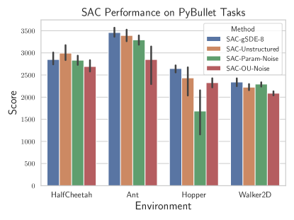
Tables 1 and 2 shows the results on the PyBullet tasks and the compromise between continuity and performance. Without any noise (“No Noise” in the figure), SAC is still able to solve partially those tasks thanks to a shaped reward, but it has the highest variance in the results. Although the correlated and parameter noise yield lower continuity cost during training, it comes at a cost of performance. gSDE is able to achieve a good compromise between unstructured exploration and correlated noise by making use of the noise repeat parameter. gSDE-8 (sampling the noise every 8 steps) even achieves better performance with a lower continuity cost at train time. Such behavior is what is desirable for training on a real robot: we must minimize wear-and-tear at training while still obtaining good performance at test time.

4.2 Comparison to the Original SDE

In this section, we investigate the contribution of the proposed modifications to the original SDE: sampling the exploration function parameters every $n$ steps and using policy features as input to the noise function.

(a) Exploration function input

(b) Sampling interval (PPO on Walker2D)

Figure 3: Impact of gSDE modifications over the original SDE on PyBullet tasks. (a) Influence of the input to the exploration function $\epsilon(\mathbf{s};\theta_{\epsilon})$ for SAC and PPO: using latent features from the policy $\mathbf{z_{\mu}}$ (Latent) is usually better than using the state $\mathbf{s}$ (Original). (b) The frequency of sampling the noise function parameters is crucial for PPO with gSDE.

Sampling Interval

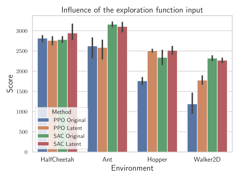
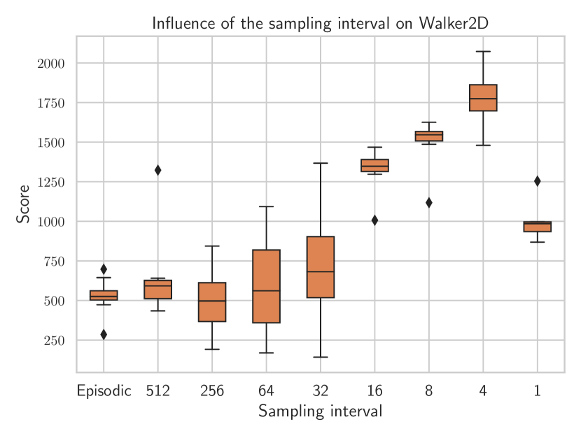
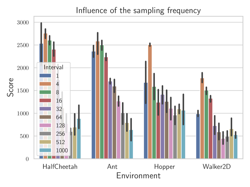
gSDE is a $n$-step version of SDE, where $n$ allows interpolating between the unstructured exploration $n=1$ and the original SDE per-episode formulation. This interpolation allows to have a compromise between performance and smoothness at train time (cf. Tables 1 and 2). Fig. 3 shows the importance of that parameter for PPO on the Walker2D task. If the sampling interval is too large, the agent would not explore enough during long episodes. On the other hand, with a high sampling frequency $n\approx 1$, the issues mentioned in Sect. 1 arise.

Policy features as input

Fig. 3 shows the effect of changing the exploration function input for SAC and PPO. Although it varies from task to task, using policy features (“latent” in the figure) is usually beneficial, especially for PPO. It also requires less tuning and no normalization as it depends only on the policy network architecture. Here, the PyBullet tasks are low dimensional and the state space size is of the same order, so no careful per-task tuning is needed. Relying on features also allows learning directly from pixels, which is not possible in the original formulation.

Compared to the original SDE, the two proposed modifications are beneficial to the performance, with the noise sampling interval $n$ having the most impact. Fortunately, as shown in Tables 1 and 2, it can be chosen quite freely for SAC. In the appendix, we provide an additional ablation study that shows gSDE is robust to the choice of the initial exploration variance.

4.3 Learning to Control a Tendon-Driven Elastic Robot

(a) Tendon-driven elastic continuum neck in a humanoid robot

(b) Model-Based controller vs RL controller on the real robot

Figure 4: (a) The tendon-driven robot [33] used for the experiment. The tendons are highlighted in orange. (b) The model-based controller and the RL agent performs similarly on an evaluation trajectory.

Experiment setup

To assess the usefulness of gSDE, we apply it on a real system. The task is to control a tendon-driven elastic continuum neck [33] (see Fig. 4) to a given target pose. Controlling such a soft robot is challenging because of the nonlinear tendon coupling, together with the deformation of the structure that needs to be modeled accurately. This modeling is computationally expensive [34, 35] and requires assumptions that may not hold in the physical system.

The system is under-actuated (there are only 4 tendons), hence, the desired pose is a 4D vector: 3 angles for the rotation $\theta_{x}$, $\theta_{y}$, $\theta_{z}$ and one for the position $x$. The input is a 16D vector composed of: the measured tendon lengths (4D), the current tendon forces (4D), the current pose (4D) and the target pose (4D). The reward is a weighted sum between the negative geodesic distance to the desired orientation and the negative Euclidean distance to the desired position. The weights are chosen such that the two components have the same magnitude. We also add a small continuity cost to reduce the oscillations in the final policy. The action space consists in desired delta in tendon forces, limited to $5\text{\,}\mathrm{N}$. For safety reasons, the tendon forces are clipped below $10\text{\,}\mathrm{N}$ and above $40\text{\,}\mathrm{N}$. An episode terminates either when the agent reaches the desired pose or after a timeout of $5\text{\,}\mathrm{s}$. The episode is considered successful if the desired pose is reached within a threshold of $10\text{\,}\mathrm{mm}$ for the position and $5\mathrm{°}$ for the orientation. The agent controls the tendons forces at $30\text{\,}\mathrm{Hz}$, while a PD controller monitors the motor current at $3\text{\,}\mathrm{kHz}$ on the robot. Gradient updates are directly done on a 4-core laptop, after each episode.

Results

We first ran the unstructured exploration on the robot, but had to stop the experiment early: the high-frequency noise in the command was damaging the tendons and would have broken them due to their friction on the bearings. Therefore, as a baseline, we trained a policy using SAC with a hand-crafted action smoothing ($2\text{\,}\mathrm{Hz}$ cutoff Butterworth low-pass filter) for two hours.
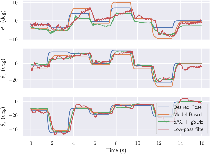
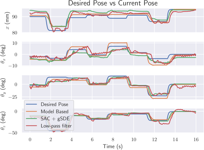
Then, we trained a controller using SAC with gSDE for the same duration. We compare both learned controllers to an existing model-based controller (passivity-based approach) presented in [34, 35] using a pre-defined trajectory (cf. Fig. 4). On the evaluation trajectory, the controllers are equally precise (cf. Table 3): the mean error in orientation is below $3\mathrm{°}$ and the one in position below $3\text{\,}\mathrm{mm}$. However, the policy trained with the low-pass filter is much more jittery than the two others. We quantify this jitter as the mean absolute difference between two timesteps, denoted as continuity cost in Table 3.

	Unstructured	gSDE	Low-pass filter	Model-Based
	noise
Position error (mm)	N/A	2.65 +/- 1.6	1.98 +/- 1.7	1.32 +/- 1.2
Orientation error (deg)	N/A	2.85 +/- 2.9	3.53 +/- 4.0	2.90 +/- 2.8
Continuity cost (deg)	N/A	0.20 +/- 0.04	0.38 +/- 0.07	0.16 +/- 0.04

Table 2: Comparison of the mean error in position, orientation and mean continuity cost on the evaluation trajectory. We highlight best approaches when the difference is significant. The model-based and learned controllers yield comparable results but the policy trained with a low-pass filter has a much higher continuity cost.

Additional Real Robot Experiments

(a) Quadruped and RC car robots

(b) Learning curve on the walking task for the quadruped robot

Figure 5: Additional robots successfully trained using SAC with gSDE directly in the real world.

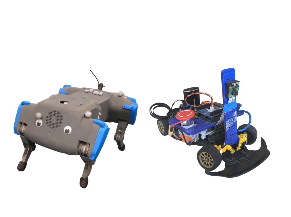
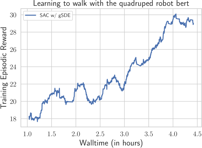
We also successfully applied SAC with gSDE on two additional real robotics tasks (see Fig. 5): training an elastic quadruped robot to walk (learning curve in Fig. 5) and learning to drive around a track using an RC car. Both experiments are fully done on the real robot, without the use of simulation nor filter. We provide in the supplementary material the videos of the trained controllers.

5 Related Work

Exploration is a key topic in reinforcement learning [36]. It has been extensively studied in the discrete case and most recent papers still focus on discrete actions [37, 38].

Several works tackle the issues of unstructured exploration for continuous control by replacing it with correlated noise. Korenkevych et al. [15] use an autoregressive process and introduce two variables that allows to control the smoothness of the exploration. In the same vein, van Hoof et al. [27] rely on a temporal coherence parameter to interpolate between the step- or episode-based exploration, making use of a Markov chain to correlate the noise. This smoothed noise comes at a cost: it requires an history, which changes the problem definition.

Exploring in parameter space [10, 39, 11, 12, 40] is an orthogonal approach that also solves some issues of the unstructured exploration. It was successfully applied to real robot but relied on motor primitives [41, 12], which requires expert knowledge. Plappert et al. [19] adapt parameter exploration to Deep RL by defining a distance in the action space and applying layer normalization to handle high-dimensional space.

Population based algorithms, such as Evolution strategies (ES) or Genetic Algorithms (GA), also explore in parameter space. Thanks to massive parallelization, they were shown to be competitive [42] with RL in terms of training time, at the cost of being sample inefficient. To address this problem, recent works [20] proposed to combine ES exploration with RL gradient update. This combination, although powerful, unfortunately adds numerous hyperparameters and a non-negligible computational overhead.

Obtaining smooth control is essential for real robot, but it is usually overlooked by the DeepRL community. Recently, Mysore et al. [14] integrated a continuity and smoothing loss inside RL algorithms. Their approach is effective to obtain a smooth controller that reduces the energy used at test time on the real robot. However, it does not solve the issue of smooth exploration at train time, limiting their training to simulation only.

6 Conclusion

In this work, we highlighted several issues that arise from the unstructured exploration in Deep RL algorithms for continuous control. Due to those issues, these algorithms cannot be directly applied to learning on real-world robots.

To address these issues, we adapt State-Dependent Exploration to Deep RL algorithms by extending the original formulation: we sample the noise every $n$ steps and replace the exploration function input by learned features. This generalized version (gSDE), provides a simple and efficient alternative to unstructured Gaussian exploration.

gSDE achieves very competitive results on several continuous control benchmarks, while reducing wear-and-tear at train time. We also investigate the contribution of each modification by performing an ablation study: the noise sampling interval has the most impact and allows a compromise between performance and smoothness. Our proposed exploration strategy, combined with SAC, is robust to hyperparameter choice, which makes it suitable for robotics applications. To demonstrate it, we successfully apply SAC with gSDE directly on three different robots.

Although much progress is being made in sim2real approaches, we believe more effort should be invested in learning directly on real systems, even if this poses challenges in terms of safety and duration of learning. This paper is meant as a step towards this goal, and we hope that it will revive interest in developing exploration methods that can be directly applied to real robots.

Appendix A Supplementary Material

A.1 State Dependent Exploration

In the linear case, i. e. with a linear policy and a noise matrix, parameter space exploration and SDE are equivalent:

$${\mathbf{a}_{t}} =\mu({\mathbf{s}_{t}};\theta_{\mu})+\epsilon({\mathbf{s}_{t}};\theta_{\epsilon}), \theta_{\epsilon}\sim\mathcal{N}(0,\sigma^{2})$$

$$=\theta_{\mu}{\mathbf{s}_{t}}+\theta_{\epsilon}{\mathbf{s}_{t}}$$

$$=(\theta_{\mu}+\theta_{\epsilon}){\mathbf{s}_{t}}$$

Because we know the policy distribution, we can obtain the derivative of the log-likelihood $\log\pi(\mathbf{a}|\mathbf{s})$ with respect to the variance $\sigma$:

$$\frac{\partial\log\pi(\mathbf{a}|\mathbf{s})}{\partial\sigma_{ij}} =\sum_{k}{\frac{\partial\log\pi_{k}(\mathbf{a}_{k}|\mathbf{s})}{\partial\hat{\sigma_{j}}}\frac{\partial\hat{\sigma}_{j}}{\partial\sigma_{ij}}}$$ (7)

$$=\frac{\partial\log\pi_{j}(\mathbf{a}_{j}|\mathbf{s})}{\partial\hat{\sigma}_{j}}\frac{\partial\hat{\sigma}_{j}}{\partial\sigma_{ij}}$$ (8)

$$=\frac{(\mathbf{a}_{j}-\mu_{j})^{2}-\hat{\sigma_{j}}^{2}}{\hat{\sigma_{j}}^{3}}\frac{\mathbf{s}_{i}^{2}\sigma_{ij}}{\hat{\sigma_{j}}}$$ (9)

This can be easily plugged into the likelihood ratio gradient estimator [26], which allows adapting $\sigma$ during training. SDE is therefore compatible with standard policy gradient methods, while addressing most shortcomings of the unstructured exploration.

A.2 Algorithms

In this section, we shortly present the algorithms used in this paper. They correspond to state-of-the-art methods in model-free RL for continuous control, either in terms of sample efficiency or wall-clock time.

A2C

A2C is the synchronous version of Asynchronous Advantage Actor-Critic (A3C) [23]. It is an actor-critic method that uses parallel rollouts of $n$-steps to update the policy. It relies on the REINFORCE [26] estimator to compute the gradient. A2C is fast but not sample efficient.

PPO

A2C gradient update does not prevent large changes that lead to huge drop in performance. To tackle this issue, Trust Region Policy Optimization (TRPO) [21] introduces a trust-region in the policy parameter space, formulated as a constrained optimization problem: it updates the policy while being close in terms of KL divergence to the old policy. Its successor, Proximal Policy Optimization (PPO) [24] relaxes the constraints (which requires costly conjugate gradient step) by clipping the objective using importance ratio. PPO makes also use of workers (as in A2C) and Generalized Advantage Estimation (GAE) [43] for computing the advantage.

TD3

Deep Deterministic Policy Gradient (DDPG) [22] combines the deterministic policy gradient algorithm [44] with the improvements from Deep Q-Network (DQN) [45]: using a replay buffer and target networks to stabilize training. Its direct successor, Twin Delayed DDPG (TD3) [5] brings three major tricks to tackle issues coming from function approximation: clipped double Q-Learning (to reduce overestimation of the Q-value function), delayed policy update (so the value function converges first) and target policy smoothing (to prevent overfitting). Because the policy is deterministic, DDPG and TD3 rely on external noise for exploration.

SAC

Soft Actor-Critic [25], successor of Soft Q-Learning (SQL) [46] optimizes the maximum-entropy objective, that is slightly different compared to the classic RL objective:

$$J(\pi)=\sum_{t=0}^{T}\operatorname{\mathbb{E}}_{({\mathbf{s}_{t}},{\mathbf{a}_{t}})\sim\rho_{\pi}}\left[r({\mathbf{s}_{t}},{\mathbf{a}_{t}})+\alpha\mathcal{H}(\pi({\,\cdot\,}|{\mathbf{s}_{t}}))\right].$$ (10)

where $\mathcal{H}$ is the policy entropy and $\alpha$ is the entropy temperature and allows to have a trade-off between the two objectives.

SAC learns a stochastic policy, using a squashed Gaussian distribution, and incorporates the clipped double Q-learning trick from TD3. In its latest iteration [8], SAC automatically adjusts the entropy coefficient $\alpha$, removing the need to tune this crucial hyperparameter.

Which algorithm for robotics?

A2C and PPO are both on-policy algorithms and can be easily parallelized, resulting in relatively small training time. On the other hand, SAC and TD3 are off-policy and run on a single worker, but are much more sample efficient than the two previous methods, achieving equivalent performances with a fraction of the samples.

Because we are focusing on robotics applications, having multiple robots is usually not possible, which makes TD3 and SAC the methods of choice. Although TD3 and SAC are very similar, SAC embeds the exploration directly in its objective function, making it easier to tune. We also found, during our experiments in simulation, that SAC works for a wide range of hyperparameters. As a result, we adopt that algorithm for the experiment on a real robot and for the ablation study.

A.3 Real Robot Experiments

Common Setup

For each real robot experiment, to improve smoothness of the final controller and tackle communication delays (which would break Markov assumption), we augment the input with the previous observation and the last action taken and add a small continuity cost to the reward. For each task, we decompose the reward function into a primary (what we want to achieve) and secondary component (soft constraints such as continuity cost). Each reward term is normalized, which allows to easily weight each component depending on their importance. Compared to previous work, we use the exact same algorithm as the one used for simulated tasks and therefore avoid the use of filter.

Learning to control an elastic neck.

An episode terminates either when the agent reaches the desired pose or after a timeout of 5s, i. e. each episode has a maximum length of 200 steps. The episode is considered successful if the desired pose is reached within a threshold of $10mm$ for the position and $5deg$ for the orientation.

Learning to walk with the elastic quadruped robot bert.

The agent receives joint angles, velocities, torques and IMU data as input (over Wi-Fi) and commands the desired absolute motor angles. The primary reward is the distance traveled and the secondary reward is a weighted sum of different costs: heading cost, distance to the center line and continuity cost. Thanks to a treadmill, the reset of the robot was semi-automated. Early stopping and monitoring of the robot was done using external tracking, but the observation is computed from on-board sensors only. An episode terminates if the robot falls, goes out of bounds or after a timeout of 5s. Training is done directly with the real robot over several days, totalizing around 8 hours of interaction.

Learning to drive with a RC car.

The agent receives an image from the on-board camera as input and commands desired throttle and steering angle. Features are computed using a pre-trained auto-encoder as in Raffin and Sokolkov [47]. The primary reward is a weighted sum between a survival bonus (no intervention by the safety driver) and the commanded throttle. There is only the continuity cost as secondary reward. One episode terminates when the safety driver intervenes (crash) or after a timeout of 1 minute. Training is done directly on the robot and requires less than 30 minutes of interaction.

Figure 6: Comparison of the model-based controller with the learned RL agent on an evaluation trajectory: the two performs similarly.

	SAC + gSDE		Model-Based [34]
Error in position (mm)	2.65 +/- 1.6		1.32 +/- 1.2
Error in orientation (deg)	2.85 +/- 2.9		2.90 +/- 2.8

Table 3: Comparison of the mean error in position and orientation on the evaluation trajectory. The model-based and learned controller yield comparable results.

A.4 Implementation Details

We used a PyTorch [31] version of Stable-Baselines [48] library, together with the RL Zoo training framework [32]. It uses the common implementations tricks for PPO [49] for the version using independent Gaussian noise.

For SAC, to ensure numerical stability, we clip the mean to be in range $[-2,2]$, as it was causing infinite values. In the original implementation, a regularization $\mathcal{L}_{2}$ loss on the mean and standard deviation was used instead. The algorithm for SAC with gSDE is described in Algorithm 1.

Compared to the original SDE paper, we did not have to use the expln trick [1] to avoid exploding variance for PyBullet tasks. However, we found it useful on specific environment like BipedalWalkerHardcore-v2. The original SAC implementation clips this variance.

Algorithm 1 Soft Actor-Critic with gSDE

Initialize parameters $\theta_{\mu}$, $\theta_{Q}$, $\sigma$, $\alpha$

Initialize replay buffer $\mathcal{D}$

for each iteration do

     $\theta_{\epsilon}\sim\mathcal{N}(0,\sigma^{2})$ $\triangleright$ Sample noise function parameters

     for each environment step do

         ${\mathbf{a}_{t}}=\pi({\mathbf{s}_{t}})=\mu({\mathbf{s}_{t}};\theta_{\mu})+\epsilon({\mathbf{s}_{t}};\theta_{\epsilon})$ $\triangleright$ Get the noisy action

         $\mathbf{s}_{t+1}\sim p(\mathbf{s}_{t+1}|{\mathbf{s}_{t}},{\mathbf{a}_{t}})$ $\triangleright$ Step in the environment

         $\mathcal{D}\leftarrow\mathcal{D}\cup\left\{({\mathbf{s}_{t}},{\mathbf{a}_{t}},r({\mathbf{s}_{t}},{\mathbf{a}_{t}}),\mathbf{s}_{t+1})\right\}$ $\triangleright$ Update the replay buffer

     end for

     for each gradient step do

         $\theta_{\epsilon}\sim\mathcal{N}(0,\sigma^{2})$ $\triangleright$ Sample noise function parameters

         Sample a minibatch from the replay buffer $\mathcal{D}$

         Update the entropy temperature $\alpha$

         Update parameters using $\nabla J_{Q}$ and $\nabla J_{\pi}$ $\triangleright$ Update actor $\mu$, critic $Q$ and noise variance $\sigma$

         Update target networks

     end for

end for

A.5 Learning Curves and Additional Results

Figure 7: Performance results for SAC with different type of exploration on PyBullet tasks

	A2C			PPO
Environments	gSDE	Gaussian		gSDE	Gaussian
HalfCheetah	2028 +/- 107	1652 +/- 94		2760 +/- 52	2254 +/- 66
Ant	2560 +/- 45	1967 +/- 104		2587 +/- 133	2160 +/- 63
Hopper	1448 +/- 163	1559 +/- 129		2508 +/- 16	1622 +/- 220
Walker2D	694 +/- 73	443 +/- 59		1776 +/- 53	1238 +/- 75

Table 4: Final performance (higher is better) of A2C and PPO on 4 environments with gSDE and unstructured Gaussian exploration. We report the mean over 10 runs of 2 million steps. For each benchmark, we highlight the results of the method with the best mean, when the difference is statistically significant.

	SAC			TD3
Environments	gSDE	Gaussian		gSDE	Gaussian
HalfCheetah	2850 +/- 73	2994 +/- 89		2578 +/- 44	2687 +/- 67
Ant	3459 +/- 52	3394 +/- 64		3267 +/- 34	2865 +/- 278
Hopper	2646 +/- 45	2434 +/- 190		2353 +/- 78	2470 +/- 111
Walker2D	2341 +/- 45	2225 +/- 35		1989 +/- 153	2106 +/- 67

Table 5: Final performance (higher is better) of SAC and TD3 on 4 environments with gSDE and unstructured Gaussian exploration. We report the mean over 10 runs of 1 million steps. For each benchmark, we highlight the results of the method with the best mean, when the difference is statistically significant.

(a) HalfCheetah

(b) Ant

(c) Hopper

(d) Walker2D

Figure 8: Learning curves for SAC with different type of exploration on PyBullet tasks. The line denotes the mean over 10 runs of 1 million steps.

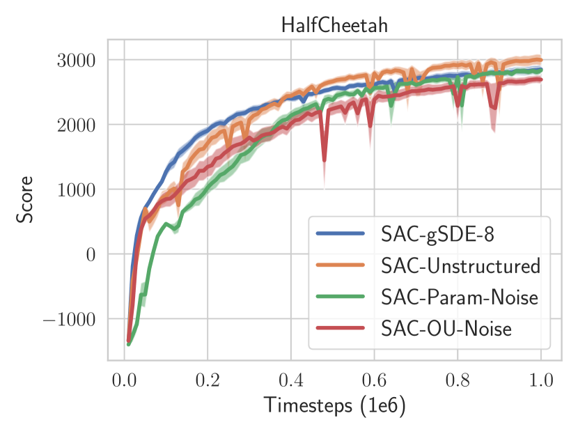
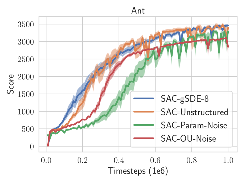
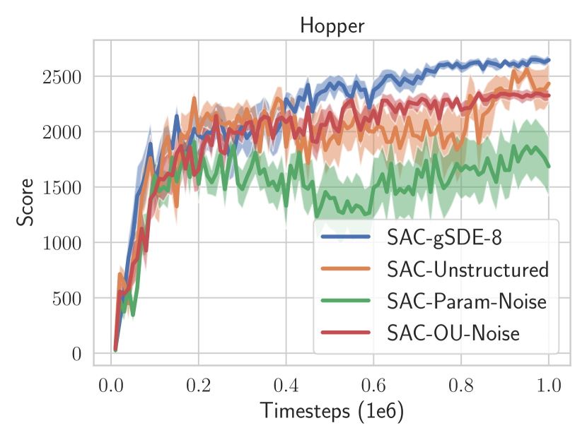
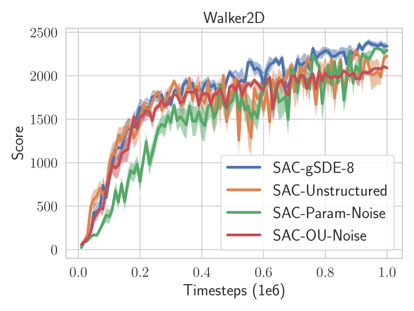
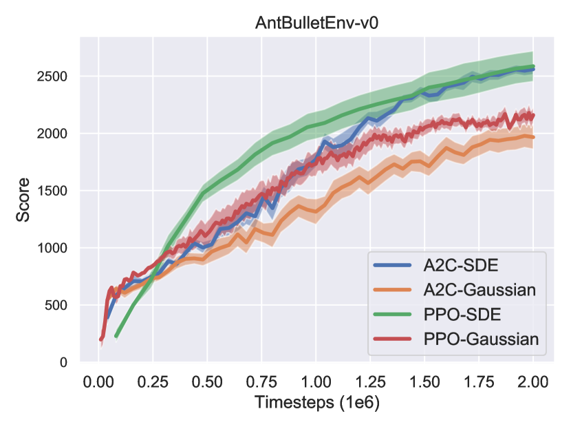
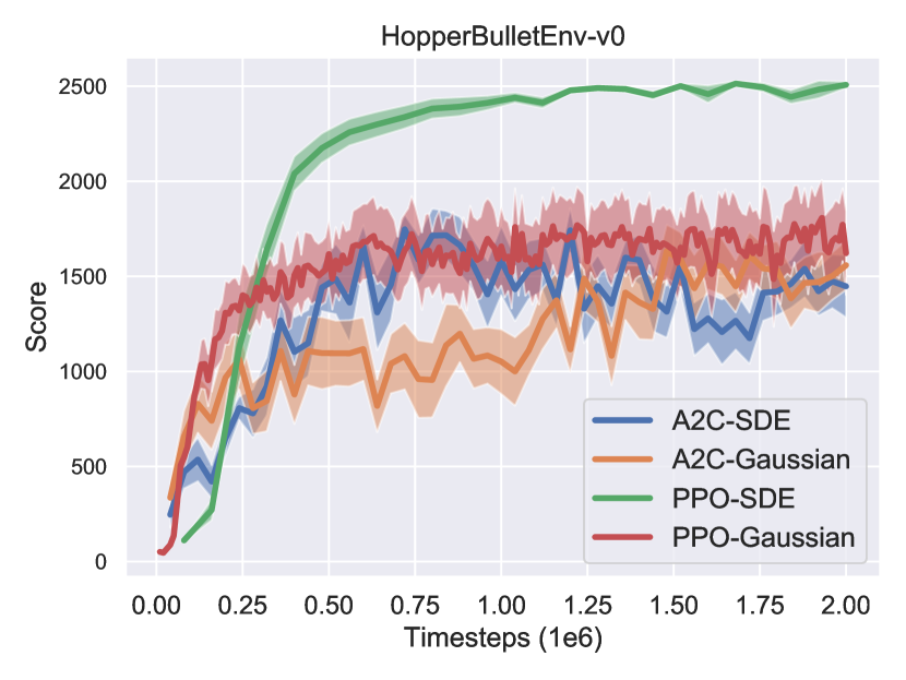
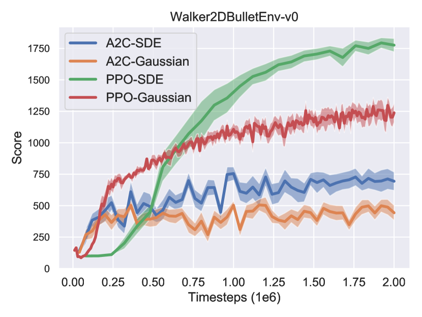
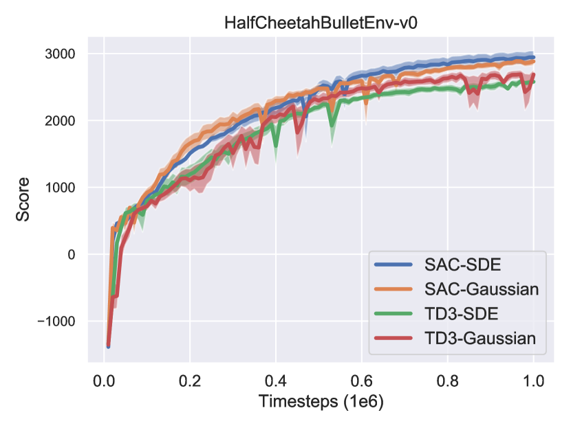
Fig. 8 shows the learning curves for SAC with different types of exploration noise.

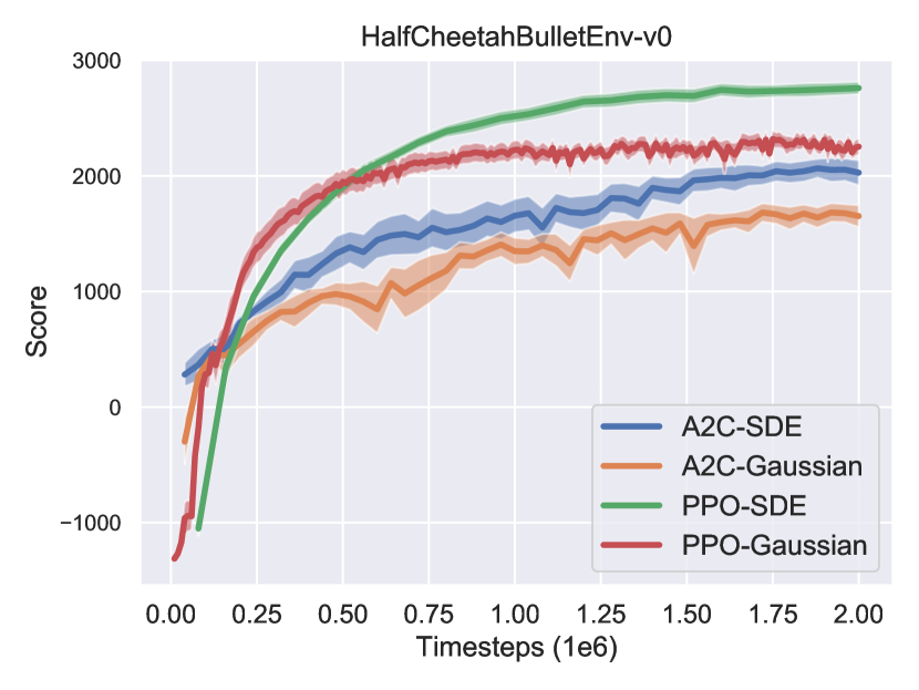
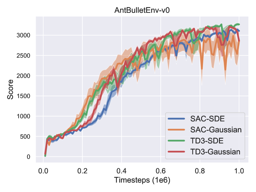
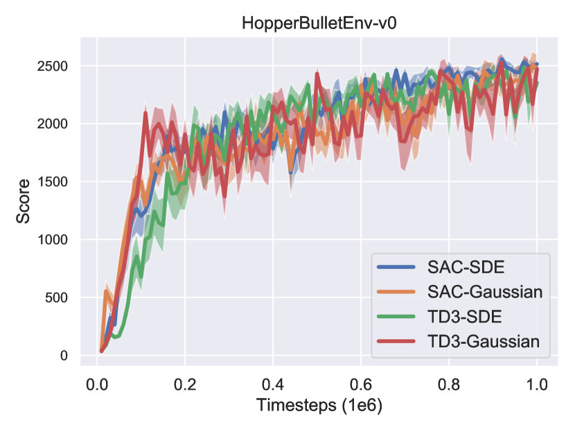
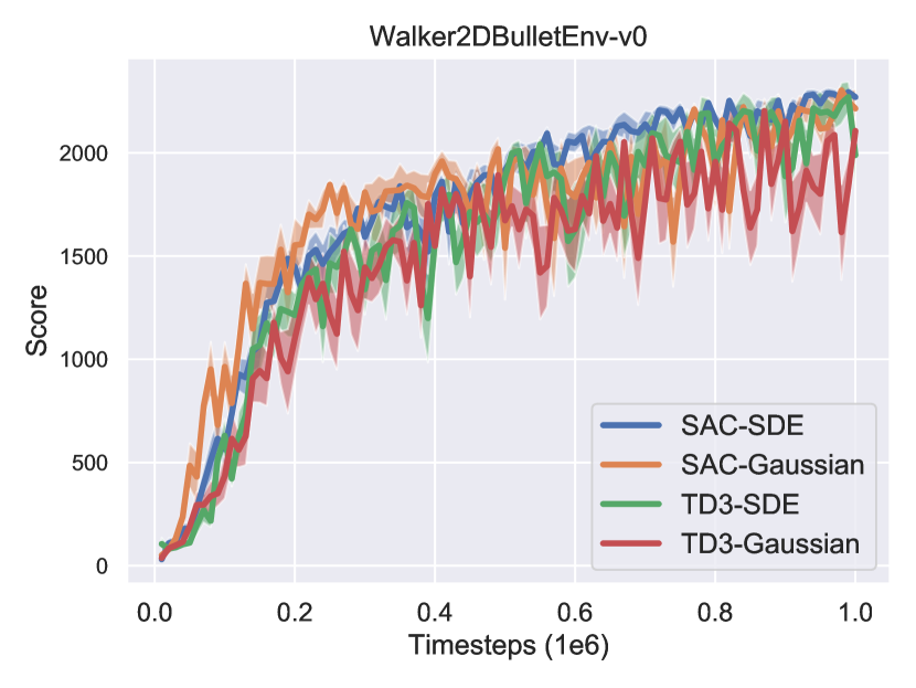
Fig. 9 and Fig. 10 show the learning curves for off-policy and on-policy algorithms on the four PyBullet tasks, using gSDE or unstructured Gaussian exploration.

(a) HalfCheetah

(b) Ant

(c) Hopper

(d) Walker2D

Figure 9: Learning curves for on-policy algorithms on PyBullet tasks. The line denotes the mean over 10 runs of 2 million steps.

(a) HalfCheetah

(b) Ant

(c) Hopper

(d) Walker2D

Figure 10: Learning curves for off-policy algorithms on PyBullet tasks. The line denotes the mean over 10 runs of 1 million steps.

A.6 Ablation Study: Additional Plots

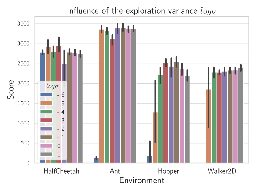
Fig. 11 displays the ablation study on remaining PyBullet tasks. It shows that SAC is robust against initial exploration variance, and PPO results highly depend on the noise sampling interval.

(a) Initial exploration variance $\log\sigma$ (SAC)

(b) Noise sampling interval (PPO)

Figure 11: Sensitivity of SAC and PPO to selected hyperparameters on PyBullet tasks

(a) Effect of parallel sampling for PPO

(b) Effect of parallel sampling for A2C

Figure 12: Parallel sampling of the noise matrix has a positive impact for PPO (a) and A2C (b) on PyBullet tasks.

Parallel Sampling

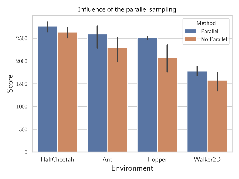
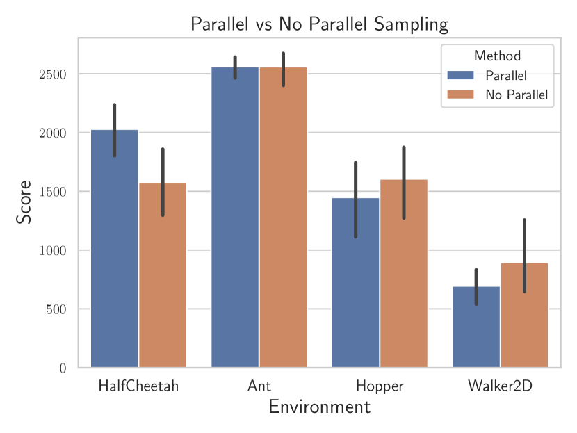
The effect of sampling a set of noise parameters per worker is shown for PPO in Fig. 12. This modification improves the performance for each task, as it allows a more diverse exploration. Although less significant, we observe the same outcome for A2C on PyBullet environments (cf. Fig. 12). Thus, making use of parallel workers improves both exploration and the final performance.

A.7 Hyperparameter Optimization

PPO and TD3 hyperparameters for unstructured exploration are reused from the original papers [24, 5]. For SAC, the optimized hyperparameters for gSDE are performing better than the ones from Haarnoja et al. [46], so we keep them for the other types of exploration to have a fair comparison. No hyperparameters are available for A2C in Mnih et al. [23] so we use the tuned one from Raffin [50].

To tune the hyperparameters, we use a TPE sampler and a median pruner from Optuna [51] library. We give a budget of 500 candidates with a maximum of $3\cdot 10^{5}$ time-steps on the HalfCheetah environment. Some hyperparameters are then manually adjusted (e. g. increasing the replay buffer size) to improve the stability of the algorithms.

A.8 Hyperparameters

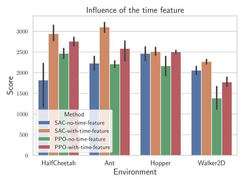
For all experiments with a time limit, as done in [3, 52, 53, 48], we augment the observation with a time feature (remaining time before the end of an episode) to avoid breaking Markov assumption. This feature has a great impact on performance, as shown in Fig. 13.

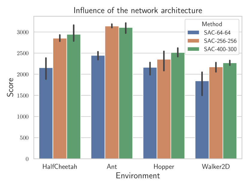
Fig. 13 displays the influence of the network architecture for SAC on PyBullet tasks. A bigger network usually yields better results but the gain is minimal passed a certain complexity (here, a two layers neural network with 256 unit per layer).

(a) Influence of the network architecture

(b) Influence of the time feature

Figure 13: (a) Influence of the network architecture (same for actor and critic) for SAC on PyBullet environments. The labels displays the number of units per layer. (b) Influence of including the time or not in the observation for PPO and SAC.

Table 6: SAC Hyperparameters

Parameter		Value
Shared
	optimizer	Adam [54]
	learning rate	$7.3\cdot 10^{-4}$
	learning rate schedule	constant
	discount ($\gamma$)	0.98
	replay buffer size	$3\cdot 10^{5}$
	number of hidden layers (all networks)	2
	number of hidden units per layer	[400, 300]
	number of samples per minibatch	256
	non-linearity	$ReLU$
	entropy coefficient ($\alpha$)	auto
	target entropy	$-dim(\mathcal{A})$
	target smoothing coefficient ($\tau$)	0.02
	train frequency	episodic
	warm-up steps	10 000
	normalization	None
gSDE
	initial $\log\sigma$	-3
	gSDE sample frequency	8

Table 7: SAC Environment Specific Parameters

Environment	Learning rate schedule
HopperBulletEnv-v0	linear
Walker2dBulletEnv-v0	linear

Table 8: TD3 Hyperparameters

Parameter		Value
Shared
	optimizer	Adam [54]
	discount ($\gamma$)	0.98
	replay buffer size	$2\cdot 10^{5}$
	number of hidden layers (all networks)	2
	number of hidden units per layer	[400, 300]
	number of samples per minibatch	100
	non-linearity	$ReLU$
	target smoothing coefficient ($\tau$)	0.005
	target policy noise	0.2
	target noise clip	0.5
	policy delay	2
	warm-up steps	10 000
	normalization	None
gSDE
	initial $\log\sigma$	-3.62
	learning rate for TD3	$6\cdot 10^{-4}$
	target update interval	64
	train frequency	64
	gradient steps	64
	learning rate for gSDE	$1.5\cdot 10^{-3}$
Unstructured Exploration
	learning rate	$1\cdot 10^{-3}$
	action noise type	Gaussian
	action noise std	0.1
	train frequency	every episode
	gradient steps	every episode

Table 9: A2C Hyperparameters

Parameter		Value
Shared
	number of workers	4
	optimizer	RMSprop with $\epsilon=1\cdot 10^{-5}$
	discount ($\gamma$)	0.99
	number of hidden layers (all networks)	2
	number of hidden units per layer	[64, 64]
	shared network between actor and critic	False
	non-linearity	$Tanh$
	value function coefficient	0.4
	entropy coefficient	0.0
	max gradient norm	0.5
	learning rate schedule	linear
	normalization	observation and reward [48]
gSDE
	number of steps per rollout	8
	initial $\log\sigma$	-3.62
	learning rate	$9\cdot 10^{-4}$
	GAE coefficient [43] ($\lambda$)	0.9
	orthogonal initialization [49]	no
Unstructured Exploration
	number of steps per rollout	32
	initial $\log\sigma$	0.0
	learning rate	$2\cdot 10^{-3}$
	GAE coefficient [43] ($\lambda$)	1.0
	orthogonal initialization [49]	yes

Table 10: PPO Hyperparameters

Parameter		Value
Shared
	optimizer	Adam [54]
	discount ($\gamma$)	0.99
	value function coefficient	0.5
	entropy coefficient	0.0
	number of hidden layers (all networks)	2
	shared network between actor and critic	False
	max gradient norm	0.5
	learning rate schedule	constant
	advantage normalization [48]	True
	clip range value function [49]	no
	normalization	observation and reward [48]
gSDE
	number of workers	16
	number of steps per rollout	512
	initial $\log\sigma$	-2
	gSDE sample frequency	4
	learning rate	$3\cdot 10^{-5}$
	number of epochs	20
	number of samples per minibatch	128
	number of hidden units per layer	[256, 256]
	non-linearity	$ReLU$
	GAE coefficient [43] ($\lambda$)	0.9
	clip range	0.4
	orthogonal initialization [49]	no
Unstructured Exploration
	number of workers	1
	number of steps per rollout	2048
	initial $\log\sigma$	0.0
	learning rate	$2\cdot 10^{-4}$
	number of epochs	10
	number of samples per minibatch	64
	number of hidden units per layer	[64, 64]
	non-linearity	$Tanh$
	GAE coefficient [43] ($\lambda$)	0.95
	clip range	0.2
	orthogonal initialization [49]	yes

Table 11: PPO Environment Specific Parameters

	Environment	Learning rate schedule	Clip range schedule	initial $\log\sigma$
gSDE
	AntBulletEnv-v0	default	default	-1
	HopperBulletEnv-v0	default	linear	-1
	Walker2dBulletEnv-v0	default	linear	default
Unstructured Exploration
	Walker2dBulletEnv-v0	linear	default	default

References

- Rückstieß et al. [2008] T. Rückstieß, M. Felder, and J. Schmidhuber. State-dependent exploration for policy gradient methods. In Joint European Conference on Machine Learning and Knowledge Discovery in Databases, pages 234–249. Springer, 2008.
- Nilsson [1984] N. J. Nilsson. Shakey the robot. Technical Report 323, Artificial Intelligence Center, SRI International, Menlo Park, CA, USA, 1984. URL http://www.ai.sri.com/shakey/.
- Duan et al. [2016] Y. Duan, X. Chen, R. Houthooft, J. Schulman, and P. Abbeel. Benchmarking deep reinforcement learning for continuous control. In International Conference on Machine Learning, pages 1329–1338, 2016.
- Andrychowicz et al. [2018] M. Andrychowicz, B. Baker, M. Chociej, R. Jozefowicz, B. McGrew, J. Pachocki, A. Petron, M. Plappert, G. Powell, A. Ray, et al. Learning dexterous in-hand manipulation. arXiv preprint arXiv:1808.00177, 2018.
- Fujimoto et al. [2018] S. Fujimoto, H. van Hoof, and D. Meger. Addressing function approximation error in actor-critic methods. arXiv preprint arXiv:1802.09477, 2018.
- Peng et al. [2018] X. B. Peng, P. Abbeel, S. Levine, and M. van de Panne. Deepmimic: Example-guided deep reinforcement learning of physics-based character skills. ACM Transactions on Graphics (TOG), 37(4):143, 2018.
- Hwangbo et al. [2019] J. Hwangbo, J. Lee, A. Dosovitskiy, D. Bellicoso, V. Tsounis, V. Koltun, and M. Hutter. Learning agile and dynamic motor skills for legged robots. arXiv preprint arXiv:1901.08652, 2019.
- Haarnoja et al. [2018] T. Haarnoja, A. Zhou, K. Hartikainen, G. Tucker, S. Ha, J. Tan, V. Kumar, H. Zhu, A. Gupta, P. Abbeel, et al. Soft actor-critic algorithms and applications. arXiv preprint arXiv:1812.05905, 2018.
- Kendall et al. [2019] A. Kendall, J. Hawke, D. Janz, P. Mazur, D. Reda, J.-M. Allen, V.-D. Lam, A. Bewley, and A. Shah. Learning to drive in a day. In 2019 International Conference on Robotics and Automation (ICRA), pages 8248–8254. IEEE, 2019.
- Kober and Peters [2009] J. Kober and J. R. Peters. Policy search for motor primitives in robotics. In Advances in neural information processing systems, pages 849–856, 2009.
- Rückstiess et al. [2010] T. Rückstiess, F. Sehnke, T. Schaul, D. Wierstra, Y. Sun, and J. Schmidhuber. Exploring parameter space in reinforcement learning. Paladyn, Journal of Behavioral Robotics, 1(1):14–24, 2010.
- Stulp and Sigaud [2013] F. Stulp and O. Sigaud. Robot skill learning: From reinforcement learning to evolution strategies. Paladyn, Journal of Behavioral Robotics, 4(1):49–61, 2013.
- Deisenroth et al. [2013] M. P. Deisenroth, G. Neumann, J. Peters, et al. A survey on policy search for robotics. Foundations and Trends® in Robotics, 2(1–2):1–142, 2013.
- Mysore et al. [2021] S. Mysore, B. Mabsout, R. Mancuso, and K. Saenko. Regularizing action policies for smooth control with reinforcement learning. 2021.
- Korenkevych et al. [2019] D. Korenkevych, A. R. Mahmood, G. Vasan, and J. Bergstra. Autoregressive policies for continuous control deep reinforcement learning. arXiv preprint arXiv:1903.11524, 2019.
- Haarnoja et al. [2018] T. Haarnoja, S. Ha, A. Zhou, J. Tan, G. Tucker, and S. Levine. Learning to walk via deep reinforcement learning. arXiv preprint arXiv:1812.11103, 2018.
- Ha et al. [2020] S. Ha, P. Xu, Z. Tan, S. Levine, and J. Tan. Learning to walk in the real world with minimal human effort. arXiv preprint arXiv:2002.08550, 02 2020.
- Neunert et al. [2020] M. Neunert, A. Abdolmaleki, M. Wulfmeier, T. Lampe, J. T. Springenberg, R. Hafner, F. Romano, J. Buchli, N. Heess, and M. Riedmiller. Continuous-discrete reinforcement learning for hybrid control in robotics. arXiv preprint arXiv:2001.00449, 2020.
- Plappert et al. [2017] M. Plappert, R. Houthooft, P. Dhariwal, S. Sidor, R. Y. Chen, X. Chen, T. Asfour, P. Abbeel, and M. Andrychowicz. Parameter space noise for exploration. arXiv preprint arXiv:1706.01905, 2017.
- Pourchot and Sigaud [2018] A. Pourchot and O. Sigaud. Cem-rl: Combining evolutionary and gradient-based methods for policy search. arXiv preprint arXiv:1810.01222, 2018.
- Schulman et al. [2015] J. Schulman, S. Levine, P. Abbeel, M. Jordan, and P. Moritz. Trust region policy optimization. In International conference on machine learning, pages 1889–1897, 2015.
- Lillicrap et al. [2015] T. P. Lillicrap, J. J. Hunt, A. Pritzel, N. Heess, T. Erez, Y. Tassa, D. Silver, and D. Wierstra. Continuous control with deep reinforcement learning. arXiv preprint arXiv:1509.02971, 2015.
- Mnih et al. [2016] V. Mnih, A. P. Badia, M. Mirza, A. Graves, T. Lillicrap, T. Harley, D. Silver, and K. Kavukcuoglu. Asynchronous methods for deep reinforcement learning. In International conference on machine learning, pages 1928–1937, 2016.
- Schulman et al. [2017] J. Schulman, F. Wolski, P. Dhariwal, A. Radford, and O. Klimov. Proximal policy optimization algorithms. arXiv preprint arXiv:1707.06347, 2017.
- Haarnoja et al. [2017] T. Haarnoja, H. Tang, P. Abbeel, and S. Levine. Reinforcement learning with deep energy-based policies. In Proceedings of the 34th International Conference on Machine Learning-Volume 70, pages 1352–1361. JMLR. org, 2017.
- Williams [1992] R. J. Williams. Simple statistical gradient-following algorithms for connectionist reinforcement learning. Machine learning, 8(3-4):229–256, 1992.
- van Hoof et al. [2017] H. van Hoof, D. Tanneberg, and J. Peters. Generalized exploration in policy search. Machine Learning, 106(9-10):1705–1724, oct 2017. Special Issue of the ECML PKDD 2017 Journal Track.
- Coumans and Bai [2016–2019] E. Coumans and Y. Bai. Pybullet, a python module for physics simulation for games, robotics and machine learning. http://pybullet.org, 2016–2019.
- Brockman et al. [2016] G. Brockman, V. Cheung, L. Pettersson, J. Schneider, J. Schulman, J. Tang, and W. Zaremba. Openai gym. arXiv preprint arXiv:1606.01540, 2016.
- Uhlenbeck and Ornstein [1930] G. E. Uhlenbeck and L. S. Ornstein. On the theory of the brownian motion. Physical review, 36(5):823, 1930.
- Raffin et al. [2019] A. Raffin, A. Hill, M. Ernestus, A. Gleave, A. Kanervisto, and N. Dormann. Stable baselines3. https://github.com/DLR-RM/stable-baselines3, 2019.
- Raffin [2020] A. Raffin. Rl baselines3 zoo. https://github.com/DLR-RM/rl-baselines3-zoo, 2020.
- Reinecke et al. [2016] J. Reinecke, B. Deutschmann, and D. Fehrenbach. A structurally flexible humanoid spine based on a tendon-driven elastic continuum. In 2016 IEEE International Conference on Robotics and Automation (ICRA), pages 4714–4721. IEEE, 2016.
- Deutschmann et al. [2017] B. Deutschmann, A. Dietrich, and C. Ott. Position control of an underactuated continuum mechanism using a reduced nonlinear model. In 2017 IEEE 56th Annual Conference on Decision and Control (CDC), pages 5223–5230. IEEE, 2017.
- Deutschmann et al. [2019] B. Deutschmann, M. Chalon, J. Reinecke, M. Maier, and C. Ott. Six-dof pose estimation for a tendon-driven continuum mechanism without a deformation model. IEEE Robotics and Automation Letters, 4(4):3425–3432, 2019.
- Sutton and Barto [2018] R. S. Sutton and A. G. Barto. Reinforcement learning: An introduction. MIT press, 2018.
- Osband et al. [2016] I. Osband, C. Blundell, A. Pritzel, and B. Van Roy. Deep exploration via bootstrapped dqn. In Advances in neural information processing systems, pages 4026–4034, 2016.
- Osband et al. [2018] I. Osband, J. Aslanides, and A. Cassirer. Randomized prior functions for deep reinforcement learning. In Advances in Neural Information Processing Systems, pages 8617–8629, 2018.
- Sehnke et al. [2010] F. Sehnke, C. Osendorfer, T. Rückstieß, A. Graves, J. Peters, and J. Schmidhuber. Parameter-exploring policy gradients. Neural Networks, 23(4):551–559, 2010.
- Sigaud and Stulp [2019] O. Sigaud and F. Stulp. Policy search in continuous action domains: an overview. Neural Networks, 2019.
- Peters and Schaal [2008] J. Peters and S. Schaal. Reinforcement learning of motor skills with policy gradients. Neural networks, 21(4):682–697, 2008.
- Such et al. [2017] F. Such, V. Madhavan, E. Conti, J. Lehman, K. Stanley, and J. Clune. Deep neuroevolution: Genetic algorithms are a competitive alternative for training deep neural networks for reinforcement learning. arXiv preprint arXiv:1712.06567, 12 2017.
- Schulman et al. [2015] J. Schulman, P. Moritz, S. Levine, M. Jordan, and P. Abbeel. High-dimensional continuous control using generalized advantage estimation. arXiv preprint arXiv:1506.02438, 2015.
- Silver et al. [2014] D. Silver, G. Lever, N. Heess, T. Degris, D. Wierstra, and M. Riedmiller. Deterministic policy gradient algorithms. In Proceedings of the 31st International Conference on International Conference on Machine Learning - Volume 32, ICML’14, page I–387–I–395. JMLR.org, 2014.
- Mnih et al. [2013] V. Mnih, K. Kavukcuoglu, D. Silver, A. Graves, I. Antonoglou, D. Wierstra, and M. Riedmiller. Playing atari with deep reinforcement learning. arXiv preprint arXiv:1312.5602, 2013.
- Haarnoja et al. [2018] T. Haarnoja, A. Zhou, P. Abbeel, and S. Levine. Soft actor-critic: Off-policy maximum entropy deep reinforcement learning with a stochastic actor. arXiv preprint arXiv:1801.01290, 2018.
- Raffin and Sokolkov [2019] A. Raffin and R. Sokolkov. Learning to drive smoothly in minutes. https://github.com/araffin/learning-to-drive-in-5-minutes/, 2019.
- Hill et al. [2018] A. Hill, A. Raffin, M. Ernestus, A. Gleave, A. Kanervisto, R. Traore, P. Dhariwal, C. Hesse, O. Klimov, A. Nichol, M. Plappert, A. Radford, J. Schulman, S. Sidor, and Y. Wu. Stable baselines. https://github.com/hill-a/stable-baselines, 2018.
- Engstrom et al. [2020] L. Engstrom, A. Ilyas, S. Santurkar, D. Tsipras, F. Janoos, L. Rudolph, and A. Madry. Implementation matters in deep {rl}: A case study on {ppo} and {trpo}. In International Conference on Learning Representations, 2020. URL https://openreview.net/forum?id=r1etN1rtPB.
- Raffin [2018] A. Raffin. Rl baselines zoo. https://github.com/araffin/rl-baselines-zoo, 2018.
- Akiba et al. [2019] T. Akiba, S. Sano, T. Yanase, T. Ohta, and M. Koyama. Optuna: A next-generation hyperparameter optimization framework. In Proceedings of the 25rd ACM SIGKDD International Conference on Knowledge Discovery and Data Mining, 2019.
- Pardo et al. [2017] F. Pardo, A. Tavakoli, V. Levdik, and P. Kormushev. Time limits in reinforcement learning. arXiv preprint arXiv:1712.00378, 2017.
- Rajeswaran et al. [2017] A. Rajeswaran, K. Lowrey, E. V. Todorov, and S. M. Kakade. Towards generalization and simplicity in continuous control. In Advances in Neural Information Processing Systems, pages 6550–6561, 2017.
- Kingma and Ba [2014] D. P. Kingma and J. Ba. Adam: A method for stochastic optimization. arXiv preprint arXiv:1412.6980, 2014.