Continuous Learning in a Single-Incremental-Task Scenario with Spike Features
Abstract.
Deep Neural Networks (DNNs) have two key deficiencies, their dependence on high precision computing and their inability to perform sequential learning, that is, when a DNN is trained on a first task and the same DNN is trained on the next task it forgets the first task. This phenomenon of forgetting previous tasks is also referred to as catastrophic forgetting. On the other hand a mammalian brain outperforms DNNs in terms of energy efficiency and the ability to learn sequentially without catastrophically forgetting. Here, we use bio-inspired Spike Timing Dependent Plasticity (STDP) in the feature extraction layers of the network with instantaneous neurons to extract meaningful features. In the classification sections of the network we use a modified synaptic intelligence that we refer to as cost per synapse metric as a regularizer to immunize the network against catastrophic forgetting in a Single-Incremental-Task scenario (SIT). In this study, we use MNIST handwritten digits dataset that was divided into five sub-tasks.
1. Introduction
Typically, Spiking Neural Networks (SNNs) are trained using an unsupervised algorithm called Spike Timing Dependant Plasticity (STDP) (Kheradpisheh et al., 2018). Spike features extracted from latency encoded convolutional variants of SNNs have been used with an SVM (Kheradpisheh et al., 2018) and a linear neural network classifier (Vaila et al., 2019) to achieve classification accuracies in excess of . However, SNNs tend to achieve lower classification accuracies when compared to Artificial Neural Networks (ANNs) (Panda et al., 2019). ANNs are trained using Stochastic Gradient Descent (SGD). The main assumption of SGD is that the mini-batches of the training data contain approximately equal number of data points with the same labels (i.e., the data is uniformly randomly distributed). This assumption does not hold for many of the machine learning systems that learn online continuously. Different kinds of continuous learning schemes have been proposed to mitigate the problem of catastrophic forgetting. Two main scenarios of continuous learning are the Multi-Task (MT) and the Single-Incremental-Task (SIT) scenarios (Maltoni and Lomonaco, 2019). In the MT scenario a neural network with a disjoint set of output neurons is used to train/test a corresponding set of disjoint tasks. In contrast, a neural network for the SIT scenario expands the number of neurons in the output layer to accommodate new classification tasks. The MT scenario is useful when training different classification tasks on the same network thereby allowing resource sharing. The SIT scenario is useful for online continuous learning applications. That is, the SIT scenario is more suitable for online machine learning systems and is more difficult compared to the MT scenario. This is because the MT network has to not only mitigate catastrophic forgetting, but also learn to differentiate classes that are usually not seen together (unless the system has some kind of short term memory to be replayed later). Self-Organizing Maps (SOM) with short-term memory were used in (Gepperth and Karaoguz, 2016) (Parisi et al., 2019) to achieve an accuracy of on the MNIST dataset using a SIT scenario and replaying the complete dataset. Using STDP based unsupervised learning and dopaminergic plasticity modulation controlled forgetting was proposed in (Allred and Roy, 2020). It was shown to achieve a accuracy on MNIST dataset using the SIT scenario. Unsupervised spiking networks with predictive coding have been trained with STDP and shown to achieve an accuracy of on the MNIST dataset using the MT scenario (Ororbia, 2019). In our work here, our network classifies the data according to the AR1 method given in (Maltoni and Lomonaco, 2019). This uses the SIT scenario which was inspired by synaptic intelligence for the MT scenario in (Zenke et al., 2017). In our previous work (Vaila et al., 2019) we used the MNIST dataset split into two disjoint tasks to show that features extracted from a spiking convolutional network (SCN) demonstrated more immunity to catastrophic forgetting compared to their ANN counterparts. In (Vaila et al., 2019), using early stopping, the first five output neurons were trained to classify the digits and then the remaining five output neurons were trained to classify the digits . The network was then tested on the complete test dataset (digits 0-9) and achieved a accuracy on this test data. In the work presented here we exclusively work with spike features extracted from an SCN and study the effect of continuous learning using the SIT scenario on the MNIST dataset. For this study the MNIST dataset was split into the five disjoint classification tasks . The feature classification is done unsupervised in the convolution layer (L2) while the classification is done in the latter layers using error backpropagation. Here we modify the synaptic intelligence regularizer calculation of (Zenke et al., 2017) in order to reduce the computational load.
2. Network
![[Uncaptioned image]](/html/2005.04167/assets/x1.png)
The feature extraction part of the network is same as in (Vaila et al., 2019) (Vaila et al., 2019). Input images are encoded into spikes using ON and OFF center DoG filters followed by thresholding (Kheradpisheh et al., 2018). The L2 (convolution) layer consists of 30 maps and the neurons that emerge as winners after lateral inhibition and STDP competition (Vaila et al., 2020) get to update their weights according to a simplified STDP (Kheradpisheh et al., 2018).
| (1) |
and are the spike times of the pre-synaptic (input) and the post-synaptic (output) neuron, respectively. If the input neuron spikes before the output neuron spikes, the weight is increased; otherwise the weight is decreased.111The input neuron is assumed to have spiked after the output neuron spiked. Learning refers to the change in the (synaptic) weights with and denoting the learning rate constants. These rate constants are initialized with low values and are typically increased for every 1500 input images as learning progresses (Kheradpisheh et al., 2018). This STDP rule is considered simplified because the amount of weight change doesn’t depend on the time duration between pre-synaptic and post-synaptic spikes. In this work, backpropagation is used only in the classification layers (L3-L4-L5) of the network with a single hidden layer L4.
3. Continuous Learning
By continuous learning we mean that the network in Figure 1 will start with two output neurons in L5 and be trained to classify the digits . During this training the error is backpropagated from layer L5 only as far as L3. After this training is complete two new neurons will be appended to the L5 layer and then trained to classify the digits . This is continued in the same manner for the three remaining classes . We proceed in the rest of this section to give the details of this training by specifying the cost function along with the (cost per synapse) weight regularizer. The neural network in this work has a softmax output layer which is the likelihood of the input image belonging to a particular class. Let denote the (flattened) spike features in L3 and denote the weights from L3 to the hidden layer L4. For task 1 there are two output neurons and we let denote the cross-entropy cost computed with the softmax outputs of these two neurons. For task 2 there are now four output neurons and we let denote the cross-entropy cost computed with the softmax outputs of these four neurons. The costs are defined in a similar manner. The L4 and the L5 weights are updated using SGD on mini-batches. denotes the cost of the input mini-batch for the task . are similarly defined. During training for task 1 the weights are updated as usual according to
| (2) |
After training is completed for task 1, we need to know the importance of each of the weights for and in terms of classifying the images of task 1. This is necessary because when we proceed to train on task 2 these ”important” weights should not be allowed to change significantly. That is the network must be forced to use the other weights for the training of task 2. Accordingly, we next define a cost per synapse regularizer during the training of task 2 to help prevent changes to the so called important weights of the task 1. The change in the cost per each synapse is defined as
| (3) |
with
| (4) |
For each task there are mini-batches with images per mini-batch for a total of input images for each task. The average change in cost for is given by
| (5) |
with
| (6) |
A softmax output layer with a cross-entropy cost function and one-hot encoded labels is the same as the log-likelihood cost function (Nielsen, 2015). The MNIST label with corresponds to the output neuron with , respectively. Let denote the images and corresponding labels in the mini-batch. In Equation (5) the average cost for mini-batch is
| (7) |
as and for . Here L5 indicates the last layer and indicates softmax output activations. Substituting Equation (7) in to Equation (5), Equation (6) becomes
| (8) |
In (Kirkpatrick et al., 2017) the authors state that near a minimum of the cost the component of Equation (8) given by is the same as
| (9) |
with some limitations (Kunstner et al., 2019) and is the Fisher information (Chiasson, 2013) for the parameter is a measure of the “importance” of the weight A large value of implies that small changes in the value of will lead to a large increase in average cost (classification error). When the network is to train for task 2, those weights with a large computed from task 1 must now be constrained to only small changes so the network will continue to classify the images of task 1 correctly. That is, when training on task 2, the network must be forced to (essentially) use only those weights that had a small value of from task 1. So, the cost per synapse for the first task (calculated during the last epoch of training for the first task) gives the relative importance of the weights for the task1 classification problem.
Let be the change in weights during the last epoch of task 1. Further denotes the value of the weights after training on task 1. The second task is trained using the regularized cost function given by
| (10) |
with
| (11) |
where and represent the Hadamard product and division, respectively. is a small positive number added to each element of the matrix to prevent division by zero when doing Hadamard division. Similarly, is calculated during the last epoch of training task , denotes the change in the weights during the last epoch, and finally denotes the weights at the end of training task . Task is trained by adding a weight regularizing term to prevent the ”important” weights from the previous tasks being changed significantly. With a matrix of zeros define
| (12) |
then we can write the cost function of the as
| (13) |
are the weights between L3 and L4 layers at the end of task and is the number of input images. Remark Note that only the weights connecting L3 to L4 are subject to cost per synapse regularization. The weights connecting L4 to L5 are trained without regularization and use the AR1 method to train sequentially (Maltoni and Lomonaco, 2019). The parameter updates for the cost function are
| (14) |
In (Zenke et al., 2017) the cost per synapse is calculated over all the

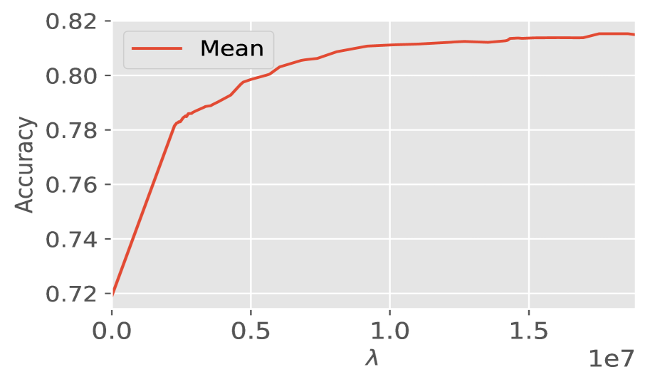
training epochs (rather than just the last epoch). The parameter in Equation (14) was optimized with validation data. Figure 2 shows the effect of on accuracy. Results for each were obtained from different weight initializations.
3.1. Results with Disjoint Tasks
In this section the network was not presented with any

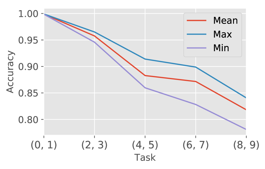
of the data from the previous tasks. Figure 3 shows the trend of testing accuracy as the network is trained on disjoint tasks with 10 different weight initializations. The highest testing accuracy achieved for this disjointly trained tasks was . was set to . in Figure 3 ’Max’ in the legend indicates the weight initialization that resulted in highest test accuracy and ’Min’ indicates the weight initialization that resulted in lowest test accuracy.
3.2. Results by Replaying
Here the data for the new task was expanded with of

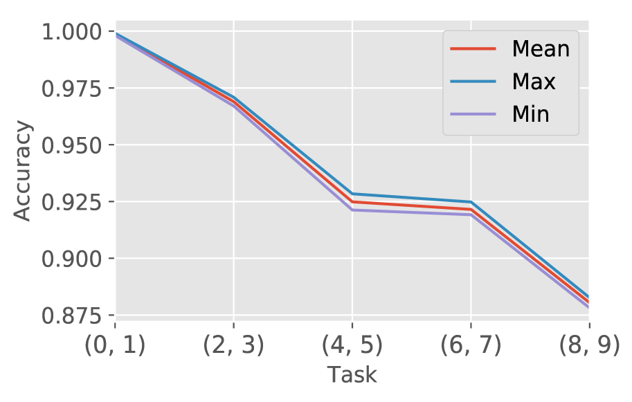
data from all the previously trained tasks. The accuracy trend as the learning progresses is shown in the Figure 4 for 10 different weight initializations with same as the disjoint case. The highest accuracy achieved by replaying of the data from the previous tasks was . For all of the above reported experiments the hyper-parameter , the mini-batch size and the number of mini-batches per task .
4. Conclusion
We achieved a final accuracy of in sequential training of MNIST dataset. While we do not claim state-of-the-art classification accuracy we proposed a hybrid method that combines bio-inspired feature extraction and the cost per synapse metric that is scalable to more challenging datasets. This is a work in progress and we are currently working towards extending this work to a more challenging EMNIST dataset (Cohen et al., 2017) by using surrogate gradients (Vaila et al., 2020) that can potentially eliminate floating point matrix-vector multiplications when implemented in a custom hardware.
References
- (1)
- Allred and Roy (2020) Jason M. Allred and Kaushik Roy. 2020. Controlled Forgetting: Targeted Stimulation and Dopaminergic Plasticity Modulation for Unsupervised Lifelong Learning in Spiking Neural Networks. Frontiers in Neuroscience 14 (2020), 7. https://doi.org/10.3389/fnins.2020.00007
- Chiasson (2013) John Nelson. Chiasson. 2013. Introduction to probability theory and stochastic processes. Wiley.
- Cohen et al. (2017) Gregory Cohen, Saeed Afshar, Jonathan Tapson, and André van Schaik. 2017. EMNIST: an extension of MNIST to handwritten letters. arXiv e-prints, Article arXiv:1702.05373 (Feb. 2017), arXiv:1702.05373 pages. arXiv:cs.CV/1702.05373
- Gepperth and Karaoguz (2016) Alexander Gepperth and Cem Karaoguz. 2016. A Bio-Inspired Incremental Learning Architecture for Applied Perceptual Problems. Cognitive Computation 8, 5 (01 Oct 2016), 924–934. https://doi.org/10.1007/s12559-016-9389-5
- Kheradpisheh et al. (2018) Saeed Reza Kheradpisheh, Mohammad Ganjtabesh, Simon J. Thorpe, and Timothée Masquelier. 2018. STDP-based spiking deep convolutional neural networks for object recognition. Neural Networks 99 (2018), 56 – 67. https://doi.org/10.1016/j.neunet.2017.12.005
- Kirkpatrick et al. (2017) James Kirkpatrick, Razvan Pascanu, Neil Rabinowitz, Joel Veness, Guillaume Desjardins, Andrei A. Rusu, Kieran Milan, John Quan, Tiago Ramalho, Agnieszka Grabska-Barwinska, Demis Hassabis, Claudia Clopath, Dharshan Kumaran, and Raia Hadsell. 2017. Overcoming catastrophic forgetting in neural networks. Proceedings of the National Academy of Sciences 114, 13 (2017), 3521–3526. https://doi.org/10.1073/pnas.1611835114 arXiv:https://www.pnas.org/content/114/13/3521.full.pdf
- Kunstner et al. (2019) Frederik Kunstner, Lukas Balles, and Philipp Hennig. 2019. Limitations of the Empirical Fisher Approximation for Natural Gradient Descent. arXiv:cs.LG/1905.12558
- Maltoni and Lomonaco (2019) Davide Maltoni and Vincenzo Lomonaco. 2019. Continuous learning in single-incremental-task scenarios. Neural Networks 116 (2019), 56 – 73. https://doi.org/10.1016/j.neunet.2019.03.010
- Nielsen (2015) Michael A Nielsen. 2015. Neural Networks and Deep Learning. Determination Press. http://neuralnetworksanddeeplearning.com/
- Ororbia (2019) Alexander Ororbia. 2019. Spiking Neural Predictive Coding for Continual Learning from Data Streams. arXiv:cs.NE/1908.08655
- Panda et al. (2019) Priyadarshini Panda, Aparna Aketi, and Kaushik Roy. 2019. Towards Scalable, Efficient and Accurate Deep Spiking Neural Networks with Backward Residual Connections, Stochastic Softmax and Hybridization. arXiv:cs.CV/1910.13931
- Parisi et al. (2019) German I. Parisi, Ronald Kemker, Jose L. Part, Christopher Kanan, and Stefan Wermter. 2019. Continual lifelong learning with neural networks: A review. Neural Networks 113 (2019), 54 – 71. https://doi.org/10.1016/j.neunet.2019.01.012
- Vaila et al. (2019) Ruthvik Vaila, John Chiasson, and Vishal Saxena. 2019. Deep Convolutional Spiking Neural Networks for Image Classification. arXiv e-prints, Article arXiv:1903.12272 (Mar 2019), arXiv:1903.12272 pages. arXiv:cs.NE/1903.12272
- Vaila et al. (2019) Ruthvik Vaila, John Chiasson, and Vishal Saxena. 2019. Feature Extraction Using Spiking Convolutional Neural Networks. In Proceedings of the International Conference on Neuromorphic Systems (ICONS ’19). Association for Computing Machinery, New York, NY, USA, Article Article 14, 8 pages. https://doi.org/10.1145/3354265.3354279
- Vaila et al. (2020) Ruthvik Vaila, John Chiasson, and Vishal Saxena. 2020. A Deep Unsupervised Feature Learning Spiking Neural Network with Binarized Classification Layers for EMNIST Classification. arXiv:cs.NE/2002.11843
- Zenke et al. (2017) Friedemann Zenke, Ben Poole, and Surya Ganguli. 2017. Continual Learning Through Synaptic Intelligence. In Proceedings of the 34th International Conference on Machine Learning (Proceedings of Machine Learning Research), Doina Precup and Yee Whye Teh (Eds.), Vol. 70. PMLR, International Convention Centre, Sydney, Australia, 3987–3995. http://proceedings.mlr.press/v70/zenke17a.html