Effect of The Latent Structure on Clustering with GANs

Abstract

Generative adversarial networks (GANs) have shown remarkable success in generation of data from natural data manifolds such as images. In several scenarios, it is desirable that generated data is well-clustered, especially when there is severe class imbalance. In this paper, we focus on the problem of clustering in generated space of GANs and uncover its relationship with the characteristics of the latent space. We derive from first principles, the necessary and sufficient conditions needed to achieve faithful clustering in the GAN framework: (i) presence of a multimodal latent space with adjustable priors, (ii) existence of a latent space inversion mechanism and (iii) imposition of the desired cluster priors on the latent space. We also identify the GAN models in the literature that partially satisfy these conditions and demonstrate the importance of all the components required, through ablative studies on multiple real world image datasets. Additionally, we describe a procedure to construct a multimodal latent space which facilitates learning of cluster priors with sparse supervision. The code for the implementation can be found at https://github.com/NEMGAN/NEMGAN-P

I Introduction

I-A Background and Contributions

Generative Adversarial Networks(GANs) [11, 1, 23, 4, 22] and its variants are a category of highly successful generative neural models which learn mappings from arbitrary latent distributions to highly complex real-world distributions. In several downstream tasks such as conditional generation, data augmentation and class balancing  [14, 3, 25, 17, 6], it is desirable that the data generated by a generative model is clustered. However, it is well known that GANs in their raw formulation are unable to fully impose all the cluster properties of the real-data on to the generated data [2, 29, 15, 4], especially when the real-data has skewed clusters. While a lot of efforts have been devoted in past to stabilize the GAN training [26, 12, 15], little attention has been given to understand the impact of latent space characteristics on data generation (a brief review of related methods is given in Sec. 4). Motivated by these observations, we propose to accomplish the following:

1. Starting from the first principles, formulate the necessary and sufficient conditions needed for faithful clustering in the generated space of GAN.

2. Demonstrate the importance of each of the condition through ablative studies using different GAN models that partially satisfy them, on four large-scale datasets.

3. Propose a method for the construction of a learnable multi-modal latent space that facilitates sparsely supervised learning of the cluster priors.

I-B Problem setting

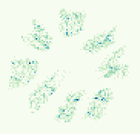
In the context of GANs, clustering in generated space refers to inheritance of the cluster properties of real data on the generated data. In GANs, a generator $g$, which is a function of the latent variable (${\mathbf{z}}$), is tasked to sample from the desired data (${\mathbf{x}}$) distribution via an adversarial game [11]. Suppose $P_{X}$ and $P_{W}$, respectively be the distributions of the generated and real data, with ${\mathbb{X}}$ and ${\mathbb{W}}$ representing their support. We call a distribution clustered (or equivalently multi-modal) if its support is a disconnected union of non-empty pairwise-disjoint connected open subsets. For instance, $P_{W}$ is a clustered distribution with $M$ clusters if ${\mathbb{W}}$ is a disconnected union of $M$ non-empty pairwise disjoint connected open subsets $\Big{(}{\mathbb{W}}_{i},i\in\{0,1,...,M-1\}\Big{)}$ and ${\mathbb{W}}\equiv\bigcup_{i=0}^{M-1}{{\mathbb{W}}}_{i}$, with ${\mathbb{W}}_{i}$ denoting the support of the $i^{th}$ mode . With this definition, clustering in generated space amounts to the following: if $P_{W}$ is clustered in the aforementioned way, $P_{X}$ is also clustered in the exact same way. That is, the probability masses of $P_{W}$ and $P_{X}$ over each individual cluster (or mode) are the same.

II Clustering in GANs - Requirements

Firstly, we show that to obtain a clustered generated space or equivalently, a multimodal $P_{X}$, it is necessary to have a multimodal latent space $P_{Z}$ with a structure similar to the real-data.

Lemma 1: Let ${\mathbb{Z}}$ denote the support of $P_{Z}$. If ${\mathbb{Z}}_{i}\subseteq{\mathbb{Z}}$ denote the inverse images of ${{\mathbb{X}}}_{i}$ under $g$, then $\bigcap_{i}{{\mathbb{X}}}_{i}=\Phi$ only if $\bigcap_{i}{{\mathbb{Z}}}_{i}=\Phi$, where $\Phi$ is an empty set.

Proof: Without the loss of generality we assume $M=2$. Assume $\displaystyle{\mathbb{X}}_{0}\cap{\mathbb{X}}_{1}=\Phi$ and $\displaystyle{\mathbb{Z}}_{0}\cap{\mathbb{Z}}_{1}\neq\Phi\implies\exists{\mathbf{z}}_{i}\in{\mathbb{Z}}_{0}\cap{\mathbb{Z}}_{1}$. Given $\displaystyle{\mathbf{z}}_{i}\in{\mathbb{Z}}_{0}$, let $g({\mathbf{z}}_{i})={\mathbf{x}}_{i0}\in{\mathbb{X}}_{0}$ and similarly, given $\displaystyle{\mathbf{z}}_{i}\in{\mathbb{Z}}_{1}$, $g({\mathbf{z}}_{i})={{\mathbf{x}}}_{i1}\in{{\mathbb{X}}}_{1}$. Since $g$ is a continuous function, ${{\mathbf{x}}}_{i0}={{\mathbf{x}}}_{i1}={{\mathbf{x}}}_{i}\implies{{\mathbf{x}}}_{i}\in{\mathbb{X}}_{0}\cap{\mathbb{X}}_{1}$ contradicting the fact that ${\mathbb{X}}_{0}\cap{\mathbb{X}}_{1}=\Phi$, hence $\displaystyle{\mathbb{Z}}_{0}\cap{\mathbb{Z}}_{1}=\Phi.$

Even though a multimodal latent space is a necessary condition (Lemma 1), it is not sufficient. The generating function $g$ can be non-injective, implying that multiple modes of the latent space can collapse to a single mode in the generated space. However, if there exists another continuous mapping $h:{{\mathbb{X}}}\rightarrow{\hat{{\mathbb{Y}}}}$ which maps the generated samples ${\mathbf{x}}$, to another auxiliary random variable $\mathbf{\hat{y}}$ such that $P_{\hat{Y}}$ is also multi-modal, then Lemma 1 can be applied again on $h$ to guarantee multimodality on $P_{X}$, as stated in the following corollary to Lemma 1.

Corollary 1.1. Let $h:{\mathbb{X}}\rightarrow\hat{{\mathbb{Y}}}$ and $\hat{{\mathbb{Y}}}_{i}\subseteq\hat{{\mathbb{Y}}}$ be a subset of $\hat{{\mathbb{Y}}}$. Then $\bigcap_{i}\hat{{\mathbb{Y}}}_{i}=\Phi$ only if $\bigcap_{i}{{\mathbb{X}}}_{i}=\Phi$. Given $\bigcap_{i}{{\mathbb{Z}}}_{i}=\Phi$, the condition $\bigcap_{i}\hat{{\mathbb{Y}}}_{i}=\Phi$ is sufficient for $\bigcap_{i}{{\mathbb{X}}}_{i}=\Phi$.

Corollary 1.1 states that if the latent distribution ($P_{Z}$) is multimodal with $M$ modes and $h$ maps ${\mathbf{x}}$ to any multimodal distribution ($P_{\hat{Y}}$) with $M$ modes, the generated distribution, $P_{X}$, will also have $M$ modes. Even though in principle, it is sufficient that if $P_{\hat{Y}}$ is any $M$ modal distribution to achieve clustering in $P_{X}$, the clusters may not be optimal as ascertained in the following corollary.

Corollary 1.2. Suppose $g$ is the generator network of a GAN which maps $P_{Z}$ to $P_{X}$ and $h$ is an inverter network which maps $P_{X}$ to $P_{\hat{Y}}$. Further, let us assume all the distributions, $P_{Z}$, $P_{X}$ and $P_{\hat{Y}}$, along with the real data distribution $P_{W}$ are multimodal with $M$ modes having disjoint supports. The cluster properties of the real data ${\mathbb{W}}$ will not be reflected in the generated data ${\mathbb{X}}$, if the probability mass under every mode (cluster) in $P_{Z}$ does not match with the modal masses of $P_{W}$ (Proof in the Supplementary material).

Thus, if either $P_{Z}$ or $P_{\hat{Y}}$ are chosen such that their mode (cluster) masses do not match with that of real data distribution $P_{W}$, the adversarial game played in the GAN objective cannot force $P_{X}$ to follow $P_{W}$. In other words, cluster properties of the real data ${\mathbb{W}}$ will not be reflected in the generated data ${\mathbb{X}}$ leading to incorrect coverage of the clusters in the generated data as observed in [16]. In summary, the following are the necessary and sufficient conditions required to accomplish clustering in the generated space of a GAN.

1. The latent space which is the input to the GAN, should be multimodal with number of modes equal to the number of clusters in the real data ($\mathbf{C_{1}}$).

2. There should be a continuous mapping from the generated space to an auxiliary multimodal random variable with same cluster properties as the real data ($\mathbf{C_{2}}$).

3. The mode (cluster) masses of the distributions of the latent and auxiliary variables must match to the mode masses of the distribution of the real data ($\mathbf{C_{3}}$).

III Clustering in GANs - Realization

In this section, we describe the possible methods for realizing the requirements for clustering with GANs.

III-A Multimodal Latent space

Two known ways of constructing a multimodal latent space are 1) using the mixture of continuous distributions such as GMM [13], 2) using the mixture of a discrete and a continuous distribution [5, 24]. Latter one is more popular and often realized by concatenation of discrete and continuous random variables. We describe a more general form of this by using an additive mixture of a pair of discrete and continuous random variables, which facilitates flexible mode priors.

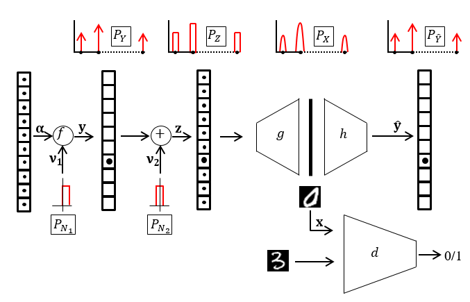
Let the latent space be represented by ${\mathbb{Z}}$ and $P_{Z}$ denote its distribution with $M$ modes. This could be obtained by taking an additive mixture of a generalized discrete distribution and a compact-support continuous distribution such as uniform distribution. Let ${\mathbf{y}}\sim P_{Y}$ and $\bm{\nu_{2}}\sim P_{N_{2}}$ denote samples drawn from the discrete and continuous distributions, respectively. Accordingly, the latent space ${\mathbf{z}}$ is obtained as: ${\mathbf{z}}={\mathbf{y}}+\bm{\nu_{2}}$. This results in a multi-modal continuous distribution with disconnected modes since $P_{Z}=P_{Y}*P_{N_{2}}$, where $*$ denotes the convolution product. The support of $P_{N_{2}}$ is chosen in such a way that the modes of $P_{Z}$ are disjoint. In $P_{Z}$, the number and the mass of the modes are obtained from discrete component $(P_{Y})$ and the continuous component $(P_{N_{2}})$ ensures variability. The discrete component ${\mathbf{y}}\sim P_{Y}$ can also be interpreted as an indicator of the modes of ${\mathbf{z}}$. Formally, ${\mathbf{y}}:=i\quad\forall{z\in{\mathbb{Z}}_{i}}$, which implies that $\int_{{\mathbb{Z}}_{i}}P_{Z}~{}d{\mathbf{z}}=P_{Y}({\mathbf{y}}=i)$.

Note that in all the aforementioned latent space construction strategies, the latent space parameters are fixed and cannot be changed or learned to suit the real-data distribution. To alleviate this problem, we propose to reparameterize a second continuous uniform distribution, $P_{N_{1}}$, using a vector $\bm{\alpha}$ to construct the desired $P_{Y}$. Let $\bm{\alpha}=[\alpha_{0},\alpha_{1},.....,\alpha_{M-1}]^{T}$, $\alpha_{i}\in\mathbb{R}$ be an arbitrary vector and $\nu_{1}\sim P_{N_{1}}(\nu_{1})=\mathbb{U}[0,1]$. We define a function, $f\left(\bm{\alpha},\nu_{1}\right):{\mathbb{R}}^{M}\times{\mathbb{R}}\rightarrow{\mathbb{R}}^{M}$ reparameterizing $P_{Y}$ as follows.

$$f_{i}\left(\alpha_{i},\nu_{1}\right)=\begin{cases}\sigma_{h}\left(a_{i}-\nu_{1}\right)-\sigma_{h}\left(a_{i-1}-\nu_{1}\right);&i\neq 0\\ \sigma_{h}\left(a_{i}-\nu_{1}\right);&i=0\end{cases}$$ (1)

where$f_{i}$ is the $i^{th}$ element of $f$, $\sigma_{h}$ is a unit step function and $a_{i}$ is given as

$$a_{i}=\frac{1}{{\sum_{k}{e^{\alpha_{k}}}}}\sum_{j=0}^{i}{e^{\alpha_{i}}}$$ (2)

With these, one can reparametrize a uniform distribution using $\bm{\alpha}$ and $f$, to obtain a multinoulli distribution.

Lemma 2: Define ${\mathbf{y}}=:\operatorname*{arg\,max}_{i\in\{0,..,M-1\}}f_{i}$, then ${\mathbf{y}}$ follows a multinoulli distribution $P_{Y}$ with

$$P_{Y}({\mathbf{y}}=i)=\frac{e^{\alpha_{i}}}{\sum_{k}{e^{\alpha_{k}}}}$$

(Proof in the supplementary material).

Therefore, starting from an arbitrary discrete valued real vector and sampling from a known uniform distribution, one can obtain a multinoulli random variable whose parameters become a function of the chosen arbitrary discrete vector $\bm{\alpha}$ which may be fixed according to the real data or learned through some inductive bias.

III-B Latent inverter

III-B1 Clustering

As mentioned in the previous sections, it is necessary to have a mapping from the generated data space to an auxiliary random variable that would have same mode masses as the real data. This can be ensured by choosing $h({{\mathbf{x}}})=\hat{{\mathbf{y}}}$ (a neural network) that would minimize a divergence measure, $\mathcal{D}(P_{\hat{Y}},P_{Y})$, such as KL-divergence, between the distribution of its output $\hat{{\mathbf{y}}}$ and the distribution of the discrete part of the latent space (${{\mathbf{y}}}$). Learning an $h$ this way, would not only lead to clustered generation, but also ensures that the modal (cluster) properties of the latent space (and thus real data) is reflected in the generated space as described in the following lemma:

Lemma 3: Let $\hat{{\mathbf{x}}}$ be a discrete random variable that is an indicator of clusters (modes) of $P_{X}$. That is, $P_{\hat{{\mathbb{X}}}}(\hat{{\mathbf{x}}}=i)=\int_{{{\mathbb{X}}}_{i}}P_{X}~{}d{\mathbf{x}}$. Then minimization of KL divergence, $D_{\mathrm{KL}}(P_{\hat{Y}}||P_{Y})$, leads to minimization of $D_{\mathrm{KL}}(P_{\hat{Y}}||P_{\hat{X}})$. (Proof given in the supplementary material).

Note that $h({\mathbf{x}})$ or $\hat{{\mathbf{y}}}$ acts like a posterior of the cluster assignment conditioned on the generated data. Therefore if the parameters of the input latent distribution ($\alpha_{i}$’s) are chosen in accordance with the modal properties of the real data distribution, generated data space will be well-clustered within a standard GAN training regime. If $g$ is the Generator of a GAN with $d$ denoting the usual discriminator network and $h$ is a neural network operating on the output of the generator to produce $\hat{{\mathbf{y}}}$, the objective function to be optimized for faithful clustering is given by:

$$\min_{g,h}\max_{d}\mathcal{L}\left(g,h,d\right)$$ (3)

$$\mathcal{L}\left(g,h,d\right)=\mathbb{E}_{{\mathbf{w}}}[\log d({\mathbf{w}})]+\mathbb{E}_{{\mathbf{z}}}[\log\left(1-d\circ g({\mathbf{z}})\right)]\\ +\mathcal{D}(P_{\hat{Y}},P_{Y})$$ (4)

where ${\mathbf{w}}$ represents samples from the real data distribution. For implementation, cross-entropy for the KL-term in equation 4 is used, since the entropy of $P_{Y}$ is a constant for a given dataset. A block diagram representing the learning pipeline is given in the Supplementary material (Fig. 2).

III-B2 Learning cluster priors

The presence of the inverter network provides an additional advantage. It helps in learning the true mode (cluster) priors in presence of a favourable inductive bias [21]. In our formulation, information about the mode-priors is parameterized through the vector $\bm{\alpha}$. Let there be a set of few labelled real data samples, call it ${\mathbb{W}}_{s}$, which provides the required inductive bias. As observed previously, the network $h({\mathbf{x}})$ is an estimator of the posterior of the cluster assignments given the data, $P(\hat{{\mathbf{y}}}|{\mathbf{x}})$. Thus, marginalizing the output of $h({\mathbf{x}})$ over all ${\mathbf{x}}$ amounts to computing $\mathbb{E}_{{\mathbf{x}}}[h({\mathbf{x}})]$, which provides an estimate of $P_{\hat{Y}}$. Analogous to $\mathbb{E}_{{\mathbf{x}}}[h({\mathbf{x}})]$, the quantity $\frac{e^{\alpha_{i}}}{\sum_{k}{e^{\alpha_{k}}}}$ provides an estimate of $P_{Y}$ (Lemma 2). If the assumed $\bm{\alpha}$ is incorrect, then $h$ would mis-assign cluster labels on some of ${\mathbb{W}}_{s}$. In other words, $P_{Y}$ and $P_{\hat{Y}}$ aren’t the same which would be the same if the priors were correct. In this scenario, we propose to retrain $h({\mathbf{x}})$ on ${\mathbb{W}}_{s}$ using a cross-entropy loss so that it assigns correct cluster labels on all of ${\mathbb{W}}_{s}$. Subsequently, we re-estimate $\mathbb{E}_{{\mathbf{x}}}[h({\mathbf{x}})]$ for an arbitrary subset of unlabelled data (typically less than 1%), with the new $h({\mathbf{x}})$. Now since $h({\mathbf{x}})$ is changed (via retraining), one can use the mismatch between $\mathbb{E}_{{\mathbf{x}}}[h({\mathbf{x}})]$ and $\frac{e^{\alpha_{i}}}{\sum_{k}{e^{\alpha_{k}}}}$ to re-compute $\bm{\alpha}$.

The following is the loss function used that incorporates the aforementioned idea for learning $\bm{\alpha}$:

$$\min_{h,\bm{\alpha}}\mathcal{L}_{\alpha}=\min_{h}\mathcal{L}_{cc}+\min_{\bm{\alpha}}\big{|}\big{|}\mathbb{E}_{{\mathbf{x}}}[h({\mathbf{x}})]-\frac{e^{\alpha_{i}}}{\sum_{k}{e^{\alpha_{k}}}}\big{|}\big{|}_{1}$$ (5)

where $\mathcal{L}_{cc}$ is the cross-entropy loss used to train $h$ on ${\mathbb{W}}_{s}$.
Note that prior-learning component is optional and independent of the GAN training which is completely unsupervised. However, since we have shown that with incorrect priors, GANs cannot cluster faithfully, the priors can be first learned, if unknown, and GANs can be trained with the correct priors.

IV GAN Models

In this section, we identify the GAN models that satisfy at-least one of the three conditions required for clustering. Vanilla GANs such as DCGAN [25], WGAN [1], SNGAN [23] etc. satisfy none of the three conditions. Models such as DeliGAN [13], GANMM [30], MADGAN [10] constructs a multimodal latent space using mixture models to avoid mode-collapse, nevertheless they neither have a latent inverter (C2) nor mode-matching (C3). Latent inverter network (with different choices for $d$) has been incorporated in the context of regularizing GAN training in many models such as VEEGAN [28], BiGAN [7], ALI [8], CATGAN [27] etc. While all of these have latent inverter with different objectives, they lack multimodal latent space (C1) and prior-matching (C3). InfoGAN [5] and ClusterGAN [24] have both multimodal latent space and latent inverter (with a mutual information maximization cost for $d$) but not the mode-matching (C3).

In the subsequent sections, we consider a representative model from all categories to demonstrate the role of all the conditions via ablations. In a model, a satisfied and an unsatisfied condition is respectively denoted with $\bf{C_{i}}$ and $\hat{C_{i}}$. For this study, we consider WGAN for $\hat{C}_{1}\hat{C}_{2}\hat{C}_{3}$, DeliGAN for $\mathbf{C_{1}}\hat{C_{2}}\hat{C}_{3}$, ALI/BiGAN for $\hat{C_{1}}\mathbf{C_{2}}\hat{C_{3}}$, InfoGAN/ClusterGAN for $\mathbf{C_{1}}\mathbf{C_{2}}\hat{C_{3}}$, and finally build a model (with WGAN as the base) with the described multimodal latent space, latent inverter (with KL-divergence for $h$) and matched prior for $\mathbf{C_{1}}\mathbf{C_{2}}\mathbf{C_{3}}$. For all the experiments, the class prior is fixed either to uniform (for $\hat{C_{3}}$) or matched to the appropriate mode/cluster prior (for $\mathbf{C_{3}}$), which provides the required inductive bias. The underlying architecture and the training procedures are kept the same across all models. All GANs are trained using the architectures and procedures described in the respective papers.

V Experiments and Results

V-A Datasets and metrics

We consider four image datasets namely, MNIST [19], FMNIST, CelebA [20], and CIFAR-10 [18] for experiments (qualitative illustration on a synthetic dataset is provided in the supplementary material, Fig. 1). Since the objective of all the experiments is to obtain a well-clustered generation with class imbalance, we create imbalanced datasets from the standard datasets by either sub-sampling or merging multiple classes. Specifically, we consider the following data - (i) take two sets of two distinct MNIST classes, 0 Vs 4 (minimal overlap under t-SNE) and 3 Vs 5 (maximum overlap under t-SNE), with two different skews of 70:30 and 90:10, (ii) merge together ‘similar’ clusters {{3,5,8}, {2}, {1,4,7,9}, {6}, {0}} to form a 5-class MNIST dataset (MNIST-5). Similarly, we also grouped FMNIST classes to create the FMNIST-5 dataset as {{Sandal, Sneaker, Ankle Boot}, {Bag}, {Tshirt/Top, Dress}, {Pullover, Coat, Shirt}, {Trouser}}, (iii) we consider CelebA dataset to distinguish celebrities with black hair from the rest. (iv) two classes of CIFAR (Frog Vs Planes, selected arbitrarily) with two synthetic imbalances of 70:30 and 90:10.

We use Accuracy (ACC), Adjusted Rand Index (ARI) and Normalized Mutual Information (NMI) [9] as metrics to measure the clustering performance and Frechet Inception Distance (FID) [23] to measure the quality of the generated images. While the first three have to be higher, FID that quantifies the relative image quality of different models, have to be lower.

V-B Results and Discussions

TABLE I: Quantitative evaluation on imbalanced data for generation with clustering. Lower performances are observed with GANs where one of three conditions is violated.

Dataset	Model	ACC	NMI	ARI	FID
	$\hat{C}_{1}\hat{C}_{2}\hat{C}_{3}$	0.64	0.06	0.08	19.76
	$\mathbf{C_{1}}\hat{C}_{2}\hat{C}_{3}$	0.66	0.13	0.11	10.14
MNIST-2	$\hat{C}_{1}\mathbf{C_{2}}\hat{C}_{3}$	0.75	0.20	0.25	15.11
(70:30)	$\mathbf{C_{1}}\mathbf{C_{2}}\hat{C}_{3}$	0.81	0.40	0.38	4.63
	$\mathbf{C_{1}}\mathbf{C_{2}}\mathbf{C_{3}}$	0.98	0.89	0.93	1.33
	$\hat{C}_{1}\hat{C}_{2}\hat{C}_{3}$	0.64	0.09	0.07	20.32
	$\mathbf{C_{1}}\hat{C}_{2}\hat{C}_{3}$	0.59	0.15	0.13	11.45
MNIST-2	$\hat{C}_{1}\mathbf{C_{2}}\hat{C}_{3}$	0.61	0.24	0.25	10.84
(90:10)	$\mathbf{C_{1}}\mathbf{C_{2}}\hat{C}_{3}$	0.77	0.33	0.54	6.08
	$\mathbf{C_{1}}\mathbf{C_{2}}\mathbf{C_{3}}$	0.98	0.86	0.91	1.66
	$\hat{C}_{1}\hat{C}_{2}\hat{C}_{3}$	0.51	0.21	0.19	20.64
	$\mathbf{C_{1}}\hat{C}_{2}\hat{C}_{3}$	0.71	0.55	0.52	12.07
MNIST-5	$\hat{C}_{1}\mathbf{C_{2}}\hat{C}_{3}$	0.76	0.59	0.64	15.31
	$\mathbf{C_{1}}\mathbf{C_{2}}\hat{C}_{3}$	0.74	0.65	0.71	4.92
	$\mathbf{C_{1}}\mathbf{C_{2}}\mathbf{C_{3}}$	0.96	0.89	0.89	1.13
	$\hat{C}_{1}\hat{C}_{2}\hat{C}_{3}$	0.62	0.30	0.30	10.46
	$\mathbf{C_{1}}\hat{C}_{2}\hat{C}_{3}$	0.77	0.66	0.61	5.41
FMNIST-5	$\hat{C}_{1}\mathbf{C_{2}}\hat{C}_{3}$	0.75	0.68	0.65	9.20
	$\mathbf{C_{1}}\mathbf{C_{2}}\hat{C}_{3}$	0.81	0.72	0.74	4.42
	$\mathbf{C_{1}}\mathbf{C_{2}}\mathbf{C_{3}}$	0.92	0.81	0.81	0.69

Results on MNIST-2 (3 Vs 5), MNIST-5 and FMNIST-5 are shown in Table I. It is observed that the GAN with all conditions satisfied (proposed) consistently outperforms the models that only satisfy the conditions partially, both in terms of cluster-purity and generation-quality. Similar observations are made on the colour datsets, CIFAR and CelebA as summerized in Table II. It is also seen that, the presence of the multimodal latent space ($C_{1}$) and a latent inverter ($C_{2}$) seem to affect the performance the most when there is class imbalance. This is corroborated by the fact that the performance of the $\mathbf{C_{1}}\mathbf{C_{2}}\hat{C}_{3}$ model (ClusterGAN) is consistently best amongst all the models that partially satisfy the conditions. This implies that knowing the class-priors is an important pre-requisite to obtain a faithful clustered generation in GANs.

Another important observation in CelebA experiment is that, different attributes e.g. eyeglasses, mustache etc., can divide the data into two clusters of different sizes. However, only black hair attribute divides the data into clusters of sizes 23.9% and 76.1% and by fixing the latent mode priors to 0.239 and 0.761, our model automatically discovers the black hair attribute and generates data accordingly. Finally, it is observed that the performance of the $\mathbf{C_{1}}\mathbf{C_{2}}\hat{C}_{3}$ and $\mathbf{C_{1}}\mathbf{C_{2}}\mathbf{C}_{3}$ are almost the same when the dataset is balanced (quantitative results in the supplementary material, Table IV). This is expected since the mode priors are matched by default in both the cases and the dataset has uniform priors. All these experiments suggests for a GAN model to generated well-clustered data, it should be equipped with all the stated conditions.

TABLE II: Evaluation of the proposed method on colour datasets, CIFAR (Frogs Vs. Planes), CelebA (black hair Vs. non-black hair). It is seen that GANs that violate any of three required conditions offer lower performance.

Dataset	Model	ACC	NMI	ARI	FID
	$\hat{C}_{1}\hat{C}_{2}\hat{C}_{3}$	0.66	0.41	0.46	55.54
	$\mathbf{C_{1}}\hat{C}_{2}\hat{C}_{3}$	0.70	0.51	0.54	42.87
CIFAR-2	$\hat{C}_{1}\mathbf{C_{2}}\hat{C}_{3}$	0.75	0.60	0.63	47.35
(70:30)	$\mathbf{C_{1}}\mathbf{C_{2}}\hat{C}_{3}$	0.72	0.68	0.65	44.38
	$\mathbf{C_{1}}\mathbf{C_{2}}\mathbf{C_{3}}$	0.88	0.70	0.75	31.15
	$\hat{C}_{1}\hat{C}_{2}\hat{C}_{3}$	0.50	0.19	0.17	58.45
	$\mathbf{C_{1}}\hat{C}_{2}\hat{C}_{3}$	0.54	0.18	0.29	43.87
CIFAR-2	$\hat{C}_{1}\mathbf{C_{2}}\hat{C}_{3}$	0.63	0.26	0.39	48.16
(90:10)	$\mathbf{C_{1}}\mathbf{C_{2}}\hat{C}_{3}$	0.67	0.22	0.21	42.01
	$\mathbf{C_{1}}\mathbf{C_{2}}\mathbf{C_{3}}$	0.83	0.26	0.28	32.86
	$\hat{C}_{1}\hat{C}_{2}\hat{C}_{3}$	0.55	0.02	0.01	150.2
	$\mathbf{C_{1}}\hat{C}_{2}\hat{C}_{3}$	0.58	0.15	0.14	110.9
CelebA	$\hat{C}_{1}\mathbf{C_{2}}\hat{C}_{3}$	0.57	0.14	0.23	83.56
	$\mathbf{C_{1}}\mathbf{C_{2}}\hat{C}_{3}$	0.64	0.18	0.26	67.1
	$\mathbf{C_{1}}\mathbf{C_{2}}\mathbf{C_{3}}$	0.81	0.30	0.38	62.9

V-C Results for Prior learning

As mentioned in Section III.A, the proposed method of latent construction with latent inverter could be used to learn the class-priors (if unknown) with sparse supervision (note that the clustering experiments are completely independent of prior-learning where the priors were assumed to be either uniform or known a-priori). To evaluate the performance of the proposed prior learning method, we consider the same setup as in the previous section, with imbalanced class priors. We initialize $\bm{\alpha}$ uniformly with same value for each of its element. Priors are learned with the technique described in Section III.B.2 using 1% of the labelled data. The learned priors are compared with real data priors in Table III. It is seen that the proposed technique learns class priors accurately for all the cases considered.

TABLE III: Evaluation of the proposed prior learning method.

Dataset	Real data priors	Learned priors
MNIST-2	[0.7, 0.3]	[0.709, 0.291]
MNIST-2	[0.9, 0.1]	[0.891, 0.109]
MNIST-5	[0.3, 0.1, 0.4,	[0.291, 0.095, 0.419,
	0.1, 0.1]	0.095, 0.099]
FMNIST-5	[0.3, 0.1, 0.3,	[0.304, 0.096, 0.284,
	0.2, 0.1]	0.220, 0.096]
CIFAR-2	[0.7, 0.3]	[0.679, 0.321]
CIFAR-2	[0.9, 0.1]	[0.876, 0.124]
CelebA-2	[0.239, 0.761]	[0.272, 0.727]

VI Conclusion

In this work, we described the problem of clustering in the generated space of GANs and investigated the role of latent space characteristics in obtaining the desired clustering. We showed, this can be achieved by having a multimodal latent space along with a latent space inversion network and matched priors of latent and real data distribution. We also proposed to parameterize the latent space such that its characteristics can be learned. It also leads to the development of a technique for learning the unknown real data class-priors using sparse supervision. Our analysis results in a GAN model which offers the advantages of robust generation under the setting of skewed data distributions and clustering, where the existing methods showed sub-optimal performances. To the best of our knowledge, this is the first work that demonstrates the importance of latent structure on the ability of GANs to generate well-clustered data.

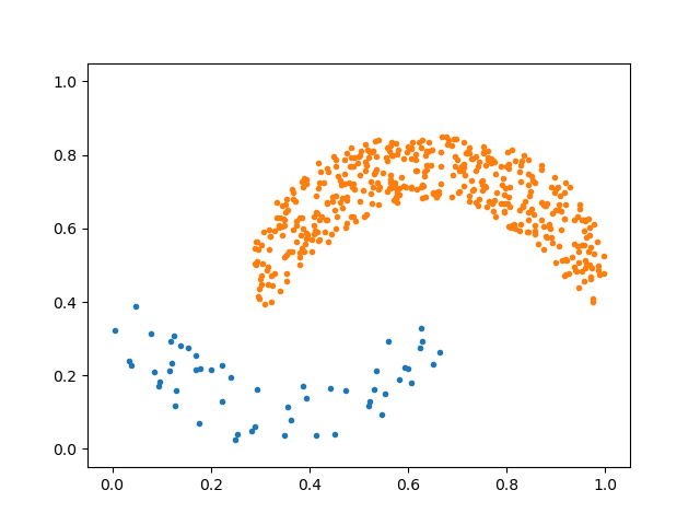
(a) Real data

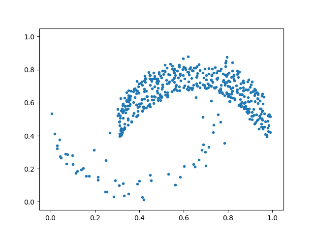
(b) WGAN

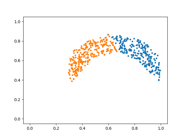
(c) DeliGAN

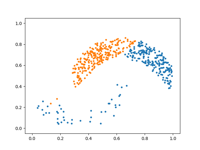
(d) InfoGAN

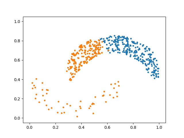
(e) ClusterGAN

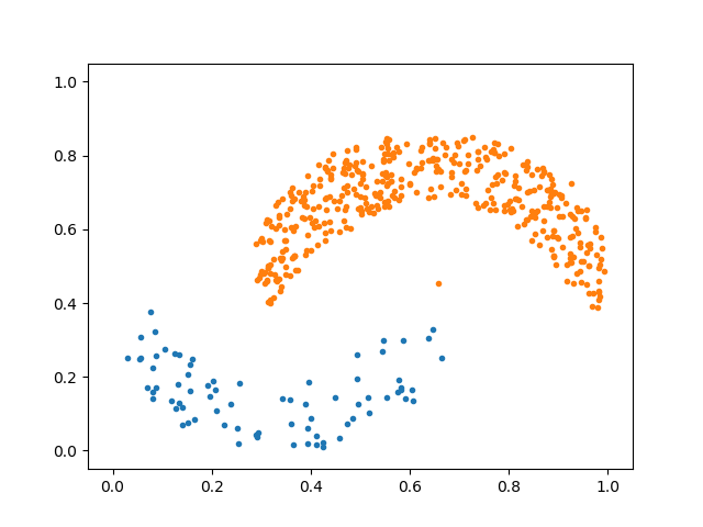
(f) Ours

Figure 1: Clustering in the generated spaces produced by different GANs for two-class Moon-data with cluster size ratio of 80:20. In absence of multimodal latent space, latent inverter and prior matching (WGAN), entire data is confined to a single cluster (Impossible conditional generation). Fulfilment of only one of the three requirements, e.g. only multimodal latent space (DeliGAN) can generate two classes but misses one of the clusters completely. Similarly the presence of multimodal latent space and latent space inverter (InfoGAN and ClusterGAN) are also unable to provide desired clustering in absence of matched priors. Our method satisfies all three conditions and thus can faithfully cluster.

Figure 2: Illustration of the proposed pipeline for clustering. Generator $g({\mathbf{z}})$ tries to mimic the real data distribution $P_{X}$ with the help of discriminator $d$. The inversion network $h(g({\mathbf{z}}))$ inverts the generation process to ensure the matching of clustering properties of generating and latent distributions. Mode priors of the latent space is encoded in ${\mathbf{y}}$ by reparameterizing a known distribution $P_{N_{1}}({\nu_{1}})$ using a learnable vector $\bm{\alpha}$.

VII Additional Proofs

Proof for Corollary 1.2: Since both $g$ and $h$ are continuous mappings (neural networks) and supports of all the distributions are disjoint,

$$\int_{{{\mathbb{Z}}}_{i}}P_{Z}~{}d{\mathbf{z}}=\int_{{{\mathbb{X}}}_{i}}P_{X}~{}d{\mathbf{x}}=\int_{{\hat{{\mathbb{Y}}}}_{i}}P_{\hat{Y}}~{}d\mathbf{\hat{y}}$$ (6)

and,

$$\int_{{{\mathbb{W}}}_{i}}P_{W}~{}d{\mathbf{w}}\neq\int_{{{\mathbb{Z}}}_{i}}P_{Z}~{}d{\mathbf{z}}\implies\int_{{{\mathbb{W}}}_{i}}P_{W}~{}d{\mathbf{w}}\neq\int_{{{\mathbb{X}}}_{i}}P_{X}~{}d{\mathbf{x}}$$ (7)

Proof for Lemma 2: Since $\sigma_{h}$ is a unit step function, $f$ is the first order difference or discrete Dirac delta function positioned at $a_{i}$. Now by definition,

$$P_{Y}({\mathbf{y}}=i)=P(f_{i}\neq 0)$$ (8)

From equation 1, we can see that $f_{i}$ becomes non-zero only for $a_{i-1}\leq\nu_{1}\leq a_{i}$, therefore,

$$P_{Y}({\mathbf{y}}=i) =P_{N_{1}}(a_{i-1}\leq\nu_{1}\leq a_{i})$$ (9)

$$=\int_{a_{i-1}}^{a_{i}}P_{N_{1}}(\nu)d\nu=a_{i}-a_{i-1}=\frac{e^{\alpha_{i}}}{\sum_{k}{e^{\alpha_{k}}}}$$ (10)

Proof for Lemma 3:

$$D_{\mathrm{KL}}(P_{\hat{Y}}||P_{Y}) =\sum_{\hat{{\mathbf{y}}}=i}{P_{\hat{Y}}}\log\frac{P_{\hat{Y}}}{P_{Y}}\quad\quad s.t.\quad i\in\{0,1\}$$ (11)

$$=\sum_{\hat{{\mathbf{y}}}=i}\left({P_{\hat{Y}}}\log{P_{\hat{Y}}}-{P_{\hat{Y}}}\log{P_{Y}}\right)$$ (12)

$$=\sum_{\hat{{\mathbf{y}}}=i}\left({P_{\hat{Y}}}\log{P_{\hat{Y}}}-{P_{\hat{Y}}}\log{\int_{{\mathbb{Z}}_{i}}P_{Z}~{}d{\mathbf{z}}}\right)$$ (13)

Since $\int_{{\mathbb{Z}}_{i}}P_{Z}~{}d{\mathbf{z}}=\int_{{\mathbb{X}}_{i}}P_{X}~{}d{\mathbf{x}}$, equation 12 can be written as

$$D_{\mathrm{KL}}(P_{\hat{Y}}||P_{Y})=\sum_{\hat{{\mathbf{y}}}=i}\left({P_{\hat{Y}}}\log{P_{\hat{Y}}}-{P_{\hat{Y}}}\log{\int_{{\mathbb{X}}_{i}}P_{X}~{}d{\mathbf{x}}}\right)$$ (14)

Since $\int_{{{\mathbb{X}}}_{i}}P_{X}~{}d{\mathbf{x}}=P_{\hat{X}}(\hat{{\mathbf{x}}}=i)$, by definition, equation 14 can be written as

$$D_{\mathrm{KL}}(P_{\hat{Y}}||P_{Y}) =\sum_{\hat{{\mathbf{y}}}=i}\left({P_{\hat{Y}}}\log{P_{\hat{Y}}}-{P_{\hat{Y}}}\log{P_{\hat{X}}}\right)$$ (15)

$$=D_{\mathrm{KL}}(P_{\hat{Y}}||P_{\hat{X}})$$ (16)

TABLE IV: Quantitative evaluation on balanced data for generation with clustering. Multimodal latent space with latent inverter offers similar performance as model with all three conditions satisfied when the data is balanced.

Dataset	Model	ACC	NMI	ARI	FID
	$\hat{C}_{1}\hat{C}_{2}\hat{C}_{3}$	0.64	0.61	0.49	10.83
	$\mathbf{C}_{1}\hat{C_{2}}\hat{C}_{3}$	0.89	0.86	0.82	8.74
MNIST	$\hat{C_{1}}\mathbf{C}_{2}\hat{C}_{3}$	0.89	0.90	0.84	7.34
	$\mathbf{C_{1}}\mathbf{C_{2}}\hat{C}_{3}$	0.95	0.89	0.89	1.84
	$\mathbf{C_{1}}\mathbf{C_{2}}\mathbf{C_{3}}$	0.96	0.91	0.92	1.82
	$\hat{C}_{1}\hat{C}_{2}\hat{C}_{3}$	0.34	0.27	0.20	19.80
	$\mathbf{C_{1}}\hat{C}_{2}\hat{C}_{3}$	0.61	0.59	0.44	12.44
FMNIST	$\hat{C_{1}}\mathbf{C}_{2}\hat{C}_{3}$	0.55	0.60	0.44	6.95
	$\mathbf{C_{1}}\mathbf{C_{2}}\hat{C}_{3}$	0.63	0.64	0.50	0.56
	$\mathbf{C_{1}}\mathbf{C_{2}}\mathbf{C_{3}}$	0.65	0.70	0.63	0.55
	$\hat{C}_{1}\hat{C}_{2}\hat{C}_{3}$	0.24	0.36	0.26	46.80
	$\mathbf{C_{1}}\hat{C}_{2}\hat{C}_{3}$	0.43	0.39	0.46	40.44
CIFAR	$\hat{C_{1}}\mathbf{C}_{2}\hat{C}_{3}$	0.52	0.42	0.48	36.95
	$\mathbf{C_{1}}\mathbf{C_{2}}\hat{C}_{3}$	0.60	0.68	0.69	29.66
	$\mathbf{C_{1}}\mathbf{C_{2}}\mathbf{C_{3}}$	0.67	0.76	0.72	26.35

VIII Additional Experiments

VIII-A D. Mode Separation

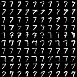
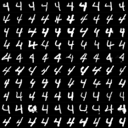
In this work, semantics of the data refer to the modes in data distribution. These semantics represent different attributes of the samples and are separated out by the proposed method. For a better understanding, experiments are conducted with samples of only a single digit type from the MNIST dataset. Samples of digit 7 and 4 are considered for this purpose. The proposed GAN ($\mathbf{C_{1}}\mathbf{C_{2}}\mathbf{C}_{3}$) is trained with a discrete uniform latent space with 10 modes and the generated images are shown in Fig. 3. Each row in Fig. 3 corresponds on one latent space mode and shows different attributes of the considered digits. For example, the fifth row in left pane contains generated images of digit 7 with slits. Similarly in right pane, the third row contains images of digit 4 with a closed notch. Note that, even with images of a single digit, no mode collapse is observed with the proposed method.

Figure 3: Demonstration of mode separation using the proposed method. Every row in each figure depicts sample from a mode when the the proposed method is trained only with a single digit type with a latent space with ten modes.

VIII-B E. Attribute discovery

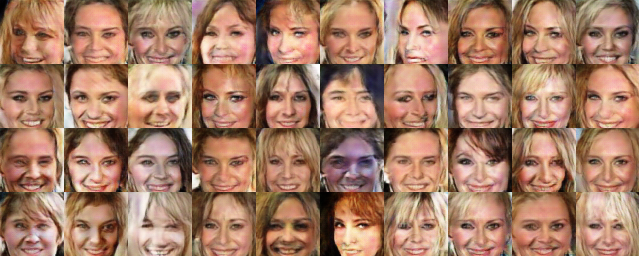
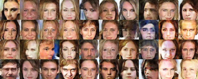
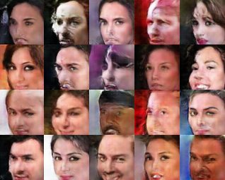
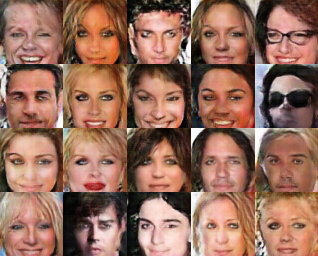
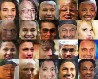
In a few real-life scenarios, the class imbalance ratio is unknown. In such cases, an unsupervised technique should discover semantically plausible regions in the data space. To evaluate the proposed method’s ability to perform such a task, we perform experiments where sample from $P_{Y}$ are drawn with an assumed class ratio rather than a known ratio. Two experiments are performed on CelebA, first with the assumption of 2 classes having a ratio of 70:30 and the second with the assumption of 3 classes having a ratio of 10:30:60. In the first experiment, the network discovers visibility of teeth as an attribute to the faces whereas in the second it learns to differentiate between the facial pose angles. Conditional generation from both the experiments are shown in figure 4 and 5, respectively. Note that these attributes are not labelled in the dataset but are discovered by our model.

Figure 4: Discovery of the facial attribute smile with teeth visible. Sample images generated in the experiments with class ratio of 70:30 for faces from the CelebA dataset.

Figure 5: Discovery of the attribute facial pose-angle. Sample images generated in the experiments with class ratio of 10:30:60 for from the CelebA dataset.

VIII-C F. Mode counting using proposed method

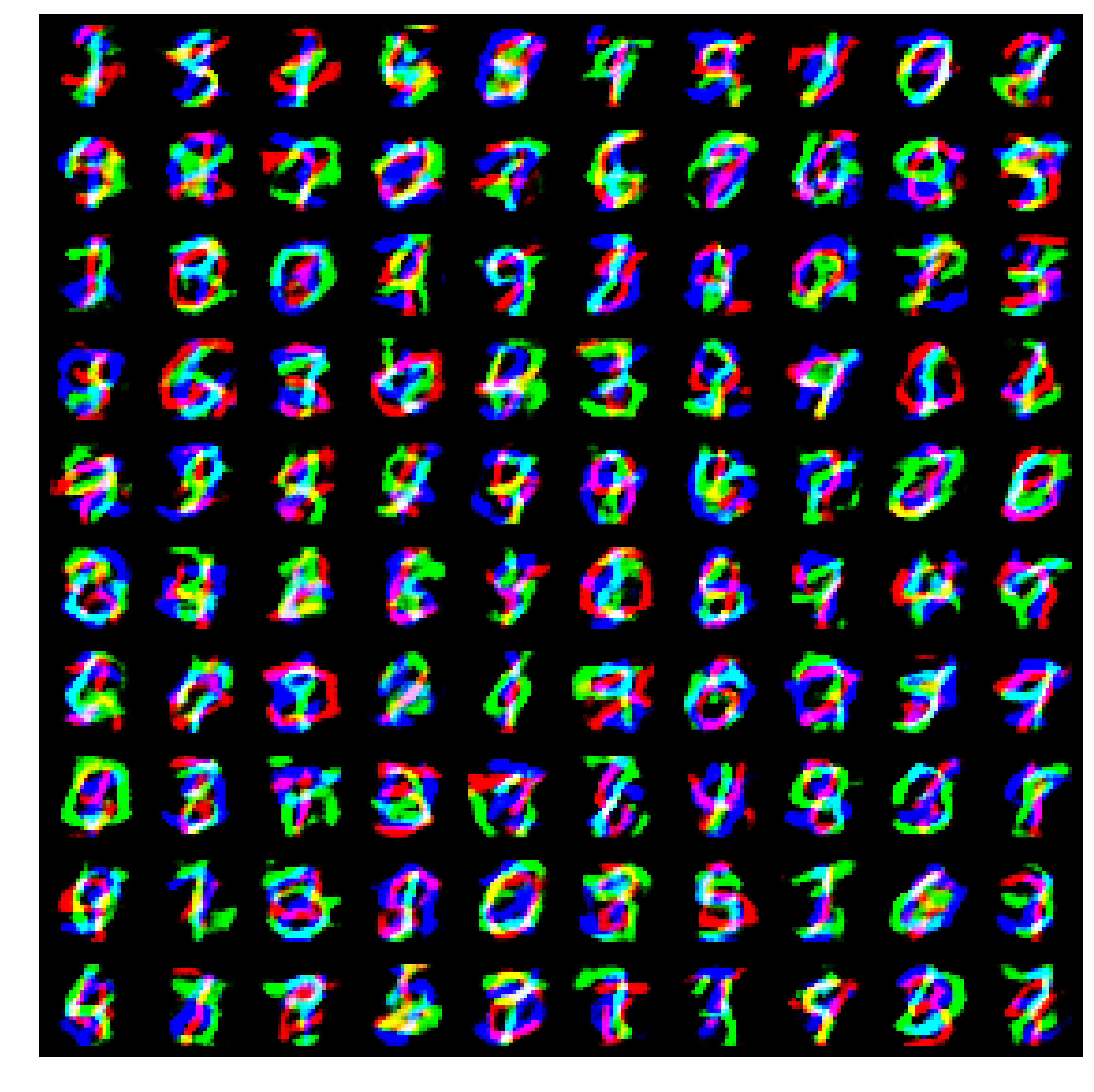
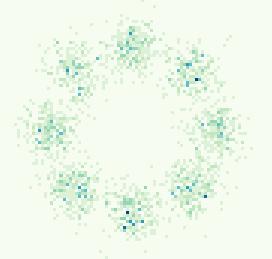
We trained the proposed method for mode counting experiment on stacked MNIST dataset. It is able to generate 993 modes. Some of the generated images are shown in Fig. 6. Similar performance is observed in 8 component GMM experiment, as shown in Fig. 7.

Figure 6: Mode counting experiment result for stacked MNIST dataset. The proposed method is able to produce variety of modes after training.

(a) Real data

(a) Generated data

Figure 7: Density plots of true data and the proposed method’s generator output for 8 component GMM arranged over a circle

References

- [1] Martin Arjovsky, Soumith Chintala, and Léon Bottou. Wasserstein generative adversarial networks. In International Conference on Machine Learning, pages 214–223, 2017.
- [2] Sanjeev Arora and Yi Zhang. Do GANs actually learn the distribution? an empirical study. arXiv preprint arXiv:1706.08224, 2017.
- [3] Yoshua Bengio, Aaron Courville, and Pascal Vincent. Representation learning: A review and new perspectives. IEEE transactions on pattern analysis and machine intelligence, 35(8):1798–1828, 2013.
- [4] Andrew Brock, Jeff Donahue, and Karen Simonyan. Large scale GAN training for high fidelity natural image synthesis. arXiv preprint arXiv:1809.11096, 2018.
- [5] Xi Chen, Yan Duan, Rein Houthooft, John Schulman, Ilya Sutskever, and Pieter Abbeel. InfoGAN: Interpretable representation learning by information maximizing generative adversarial nets. In Advances in neural information processing systems, pages 2172–2180, 2016.
- [6] Brian Cheung, Jesse A Livezey, Arjun K Bansal, and Bruno A Olshausen. Discovering hidden factors of variation in deep networks. arXiv preprint arXiv:1412.6583, 2014.
- [7] Jeff Donahue, Philipp Krähenbühl, and Trevor Darrell. Adversarial feature learning. arXiv preprint arXiv:1605.09782, 2016.
- [8] Vincent Dumoulin, Ishmael Belghazi, Ben Poole, Olivier Mastropietro, Alex Lamb, Martin Arjovsky, and Aaron Courville. Adversarially learned inference. arXiv preprint arXiv:1606.00704, 2016.
- [9] Adil Fahad, Najlaa Alshatri, Zahir Tari, Abdullah Alamri, Ibrahim Khalil, Albert Y Zomaya, Sebti Foufou, and Abdelaziz Bouras. A survey of clustering algorithms for big data: Taxonomy and empirical analysis. IEEE Transactions on Emerging Topics in Computing, 2(3):267–279, 2014.
- [10] Arnab Ghosh, Viveka Kulharia, Vinay P Namboodiri, Philip HS Torr, and Puneet K Dokania. Multi-agent diverse generative adversarial networks. In Proceedings of the IEEE Conference on Computer Vision and Pattern Recognition, pages 8513–8521, 2018.
- [11] Ian Goodfellow, Jean Pouget-Abadie, Mehdi Mirza, Bing Xu, David Warde-Farley, Sherjil Ozair, Aaron Courville, and Yoshua Bengio. Generative adversarial nets. In Advances in neural information processing systems, pages 2672–2680, 2014.
- [12] Ishaan Gulrajani, Faruk Ahmed, Martin Arjovsky, Vincent Dumoulin, and Aaron C Courville. Improved training of wasserstein GANs. In Advances in Neural Information Processing Systems, pages 5767–5777, 2017.
- [13] Swaminathan Gurumurthy, Ravi Kiran Sarvadevabhatla, and R Venkatesh Babu. DeliGAN: Generative adversarial networks for diverse and limited data. In Proceedings of the IEEE Conference on Computer Vision and Pattern Recognition, pages 166–174, 2017.
- [14] Trevor Hastie, Robert Tibshirani, and Jerome Friedman. Unsupervised learning. In The elements of statistical learning, pages 485–585. Springer, 2009.
- [15] Tero Karras, Timo Aila, Samuli Laine, and Jaakko Lehtinen. Progressive growing of GANs for improved quality, stability, and variation. arXiv preprint arXiv:1710.10196, 2017.
- [16] Mahyar Khayatkhoei, Maneesh K Singh, and Ahmed Elgammal. Disconnected manifold learning for generative adversarial networks. In Advances in Neural Information Processing Systems, pages 7343–7353, 2018.
- [17] Diederik P Kingma, Shakir Mohamed, Danilo Jimenez Rezende, and Max Welling. Semi-supervised learning with deep generative models. In Advances in Neural Information Processing Systems, pages 3581–3589, 2014.
- [18] Alex Krizhevsky and Geoffrey Hinton. Learning multiple layers of features from tiny images. Technical report, Citeseer, 2009.
- [19] Yann LeCun, Corinna Cortes, and CJ Burges. Mnist handwritten digit database. AT&T Labs [Online]. Available: http://yann. lecun. com/exdb/mnist, 2, 2010.
- [20] Ziwei Liu, Ping Luo, Xiaogang Wang, and Xiaoou Tang. Deep learning face attributes in the wild. In Proceedings of the IEEE International Conference on Computer Vision, pages 3730–3738, 2015.
- [21] Francesco Locatello, Stefan Bauer, Mario Lucic, Sylvain Gelly, Bernhard Schölkopf, and Olivier Bachem. Challenging common assumptions in the unsupervised learning of disentangled representations. arXiv preprint arXiv:1811.12359, 2018.
- [22] Xudong Mao, Qing Li, Haoran Xie, Raymond YK Lau, Zhen Wang, and Stephen Paul Smolley. Least squares generative adversarial networks. In Proceedings of the IEEE International Conference on Computer Vision, pages 2794–2802, 2017.
- [23] Takeru Miyato, Toshiki Kataoka, Masanori Koyama, and Yuichi Yoshida. Spectral normalization for generative adversarial networks. arXiv preprint arXiv:1802.05957, 2018.
- [24] Sudipto Mukherjee, Himanshu Asnani, Eugene Lin, and Sreeram Kannan. ClusterGAN: Latent space clustering in generative adversarial networks. arXiv preprint arXiv:1809.03627, 2018.
- [25] Alec Radford, Luke Metz, and Soumith Chintala. Unsupervised representation learning with deep convolutional generative adversarial networks. arXiv preprint arXiv:1511.06434, 2015.
- [26] Tim Salimans, Ian Goodfellow, Wojciech Zaremba, Vicki Cheung, Alec Radford, and Xi Chen. Improved techniques for training GANs. In Advances in Neural Information Processing Systems, pages 2234–2242, 2016.
- [27] Jost Tobias Springenberg. Unsupervised and semi-supervised learning with categorical generative adversarial networks. arXiv preprint arXiv:1511.06390, 2015.
- [28] Akash Srivastava, Lazar Valkoz, Chris Russell, Michael U Gutmann, and Charles Sutton. VEEGAN: Reducing mode collapse in GANs using implicit variational learning. In Advances in Neural Information Processing Systems, pages 3308–3318, 2017.
- [29] Huikai Wu, Shuai Zheng, Junge Zhang, and Kaiqi Huang. GP-GAN: Towards realistic high-resolution image blending. arXiv preprint arXiv:1703.07195, 2017.
- [30] Yang Yu and Wen-Ji Zhou. Mixture of GANs for clustering. In IJCAI, pages 3047–3053, 2018.