Bayesian constraints on the astrophysical neutrino source population
from IceCube data

Abstract

We present constraints on an astrophysical population of neutrino sources imposed by recent data from the IceCube neutrino observatory. By using the IceCube point source search method to model the detection of sources, our detection criterion is more sensitive than using the observation of high-energy neutrino multiplets for source identification. We frame the problem as a Bayesian hierarchical model to connect the high-level population parameters to the IceCube data, allowing us to consistently account for all relevant sources of uncertainty in our model assumptions. Our results show that sources with a local density of $n_{0}\gtrsim 10^{-7}$ $\mathrm{Mpc}^{-3}$ and luminosity $L\lesssim 10^{43}$ erg $\mathrm{s}^{-1}$ are the most likely candidates, but that populations of rare sources with $n_{0}\simeq 10^{-9}$ $\mathrm{Mpc}^{-3}$ and $L\simeq 10^{45}$ erg $\mathrm{s}^{-1}$ can still be consistent with the IceCube observations. We demonstrate that these conclusions are strongly dependent on the source evolution considered, for which we consider a wide range of models. In doing so, we present realistic, model-independent constraints on the population parameters that reflect our current state of knowledge from astrophysical neutrino observations. We also use our framework to investigate constraints in the case of possible source detections and future instrument upgrades. Our approach is flexible and can be used to model specific source cases and extended to include multi-messenger information.

I Introduction

High energy neutrinos are expected to be produced through the hadronic interactions of energetic cosmic rays with the matter and radiation fields present in their astrophysical source environments. These interactions lead to the production of charged and neutral pions, which then decay into secondary gamma rays and neutrinos [1, 2]. Thanks to extensive experimental efforts, it is now possible to detect high energy cosmic rays and neutrinos in addition to electromagnetic radiation here on Earth. These measurements provide complementary information that can be harnessed to understand their common sources. Unlike charged particles, neutrinos are weakly interacting and not deflected by intervening magnetic fields, meaning that we can use neutrino observations to identify cosmic-ray accelerators directly, as well as to study distant sources and astrophysical processes occurring within dense source environments.

A flux of high energy neutrinos ($>60$ TeV) has been measured by the IceCube Collaboration [3, 4]. These astrophysical events have been identified by their relatively high energies with respect to the atmospheric background. This signal has now been detected with high significance in both the “high energy starting events” [5] and “through-going muons” [6] channels. However, these neutrinos seem to be isotropically distributed on the sky, and various searches have not identified any point sources [7, 8, 9, 10, 11]. Due to their isotropic nature, the majority of the high energy IceCube neutrinos are thought to be of extra-Galactic origin, with a Galactic contribution constrained to $\sim$ 14% above 1 TeV [12].

Plausible extra-Galactic sources of the IceCube neutrinos are closely connected to the sources of very high energy cosmic rays with energies of up to 100 PeV, due to their production mechanism. Proposed sources include different types of active galactic nuclei and galaxies with high star formation rates as well as explosive transients such as gamma-ray bursts and tidal disruption events [13]. As neutrinos are weakly interacting and can reach us from considerable distances, the bulk of the observed high energy flux is expected to be due to the integrated contribution of many distant sources. However, for certain source population properties, we could be able to detect nearby, individual point sources in addition to this diffuse component [14]. The combination of the measurement of an astrophysical neutrino flux, but non-observation of individual neutrino sources can be used to place constraints on the properties of an unknown, steady-state source population [15, 16, 17, 18, 19, 20, 21]. The general idea is that the neutrino sources must collectively be able to satisfy the energy density requirements of the observed astrophysical flux while being consistent with the current non-detection of point sources. These simple considerations can be used to test the validity of proposed source models.

It is necessary to quantify source detection in order to place constraints on the population from the non-observation of sources. In previous work [15, 18, 19, 20, 21], this has been done by requiring a point source to produce two or more high energy ($\sim 100$–200 TeV) neutrinos in a detector. The argument is that at these energies, the angular resolution is sufficiently high, and the atmospheric neutrino background is sufficiently low, that the so-called neutrino “multiplets,” which have consistent arrival directions, must be coming from a common source. However, the probability of high-energy multiplets occurring by chance will become increasingly non-negligible as the IceCube experiment continues to gather data, meaning that it will be necessary to set even higher energy thresholds, consider only multiplets including three or more events, or make stronger corrections for the atmospheric neutrino backgrounds. All of these approaches lead to broader constraints on the source population, despite the increased detector exposure.

The goal of this work is to go beyond the multiplet assumption and model the neutrino and source detection process to characterize the detection probability in detail. We achieve this goal by connecting the high-level population parameters to observable quantities through the use of a Bayesian hierarchical model for the neutrino sources. This approach allows us to bring together the IceCube observations with a generic source population model in order to place coherent constraints on the properties of the unknown sources. In this way, the resulting constraints are summarized through the marginalized posterior distribution over the relevant parameters. Our approach also builds on previous work by including the significant effects of uncertainties in the cosmological evolution of the unknown sources and the IceCube observations, meaning that the final results reflect realistic and model-independent assumptions. We present the physical modeling assumptions in Section II, followed by a description of neutrino detection with IceCube and the characterization of the individual source detection probability in Sections III and IV. The statistical formalism for the hierarchical model that we develop is introduced in Section V. We then apply our method to recent IceCube observations in Section VI and present the results in Section VII. Finally, we summarize our framework and discuss some exciting possibilities for its extension in Section VIII. The code used in this work is open source and available online.

II Physical Model

We consider a generic, extra-Galactic population of steady, neutrino-emitting sources. Neutrinos are assumed to be produced by individual point-like sources (Section II.1), which form a population with a density distribution that evolves over cosmological scales (Section II.2). This population will produce a flux of neutrinos that can be detected on Earth (Section II.3).

II.1 Individual sources

High energy neutrinos are expected to be produced through the interactions of accelerated cosmic rays with their source environments. As such, they should have a power-law energy spectrum with a similar spectral index to that of the primary cosmic rays. We assume that the neutrino spectrum is described by a power law, such that the differential emission from a single neutrino source is given by

$$\frac{\mathrm{d}\bar{N}_{\nu}^{\mathrm{src}}}{\mathop{\mathrm{d}E}\mathop{\mathrm{d}t}}=Lk_{\gamma}E_{0}^{-\gamma}\Bigg{(}\frac{E}{E_{0}}\Bigg{)}^{-\gamma},$$ (1)

where $\mathrm{d}\bar{N}_{\nu}^{\mathrm{src}}/\mathrm{d}E\mathrm{d}t$ is the expected rate of neutrinos per unit energy, $\gamma$ is the spectral index, and $E_{0}$ is the energy at which the power law is normalized. The factor $k_{\gamma}$ is defined such that is the luminosity between $E_{\mathrm{min}}$ and $E_{\mathrm{max}}$ is given by

$$L=\int_{E_{\mathrm{min}}}^{E_{\mathrm{max}}}\mathop{\mathrm{d}E}E\frac{\mathrm{d}\bar{N}_{\nu}^{\mathrm{src}}}{\mathop{\mathrm{d}E}\mathop{\mathrm{d}t}},$$ (2)

and so we have

$$k_{\gamma}=\frac{(\gamma-2)E_{\mathrm{min}}^{\gamma-2}}{1-(E_{\mathrm{min}}/E_{\mathrm{max}})^{\gamma-2}}.$$ (3)

While this physical picture is clear for the case of sources that emit neutrinos isotropically, this assumption is expected to be false for many popular source candidate classes. For example, energetic blazars could emit neutrinos that are strongly beamed along the axis of their relativistic jets, such that all emission is contained within $\Delta\Omega$. We handle this case by considering $L$ to be the “isotropic-equivalent” luminosity, such that $L\equiv(4\pi/\Delta\Omega)L_{\mathrm{true}}$ (see e.g., Lipari [14]). We assume that all sources produce neutrinos independently of time according to their luminosity and energy spectrum.

Here, we consider all neutrino sources to have the same luminosity. While this is not realistic, this choice corresponds to more conservative constraints on the source population from the non-observation of point sources. The basic argument, as highlighted in Bartos et al. [22], is that introducing a luminosity function would increase the effective anisotropy of a population viewed from Earth, therefore making it easier to detect individual neutrino sources, and placing stronger constraints on the population for the non-observation of point sources. Additionally, the neutrino luminosity function is currently poorly constrained, given that the details of the source physics and connection to observations at other wavelengths remain open questions. However, it is potentially interesting to consider a general, parametric luminosity function that reflects our expectations. Such an extension of this model is presented in Appendix A.

II.2 The source population

We assume that individual sources are distributed isotropically throughout the universe and that their density evolves over cosmological scales. The structure of this cosmological evolution depends on the category of source candidates considered, with popular models including evolution following the star formation rate (SFR) [23] or the AGN luminosity function [24]. Flat or even negative evolutions are also often considered for comparison, motivated by studies of the ultra-high-energy cosmic ray data [25, 26, 27] and the debated evolution of certain types of BL Lac objects [28]. In order to account for the uncertainty in the exact form of the comoving density, we parameterize this as a simple function capable of representing a range of relevant source models, motivated by parameterizations used in Cole et al. [29] and Ueda et al. [30]. The expected number of sources per unit comoving volume is given by

$$\frac{\mathrm{d}\bar{N}_{\mathrm{s}}^{\mathrm{tot}}}{\mathrm{d}V}=n_{0}\frac{(1+z)^{p_{1}}}{(1+z/z_{c})^{p_{2}}}=n_{0}f(z,\theta),$$ (4)

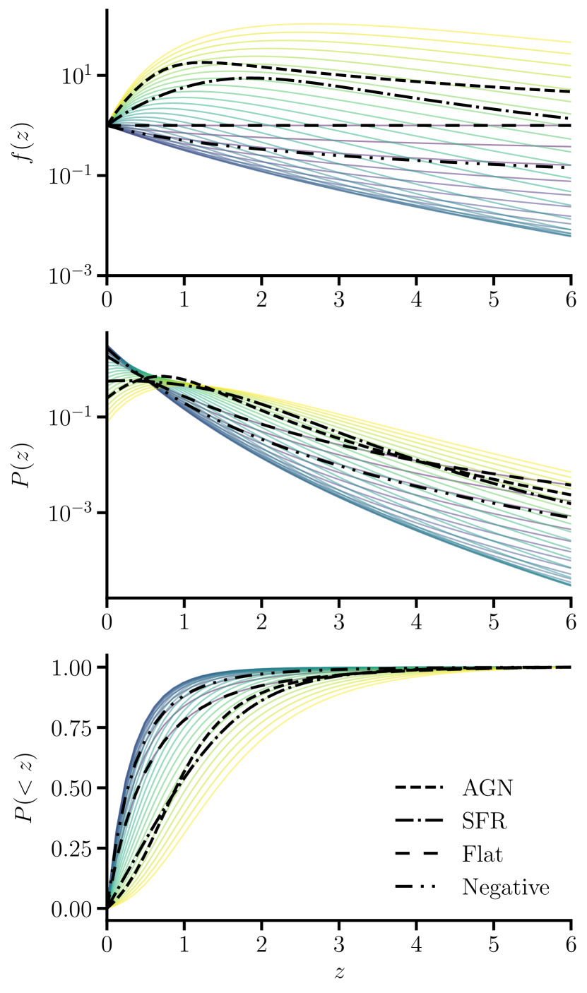
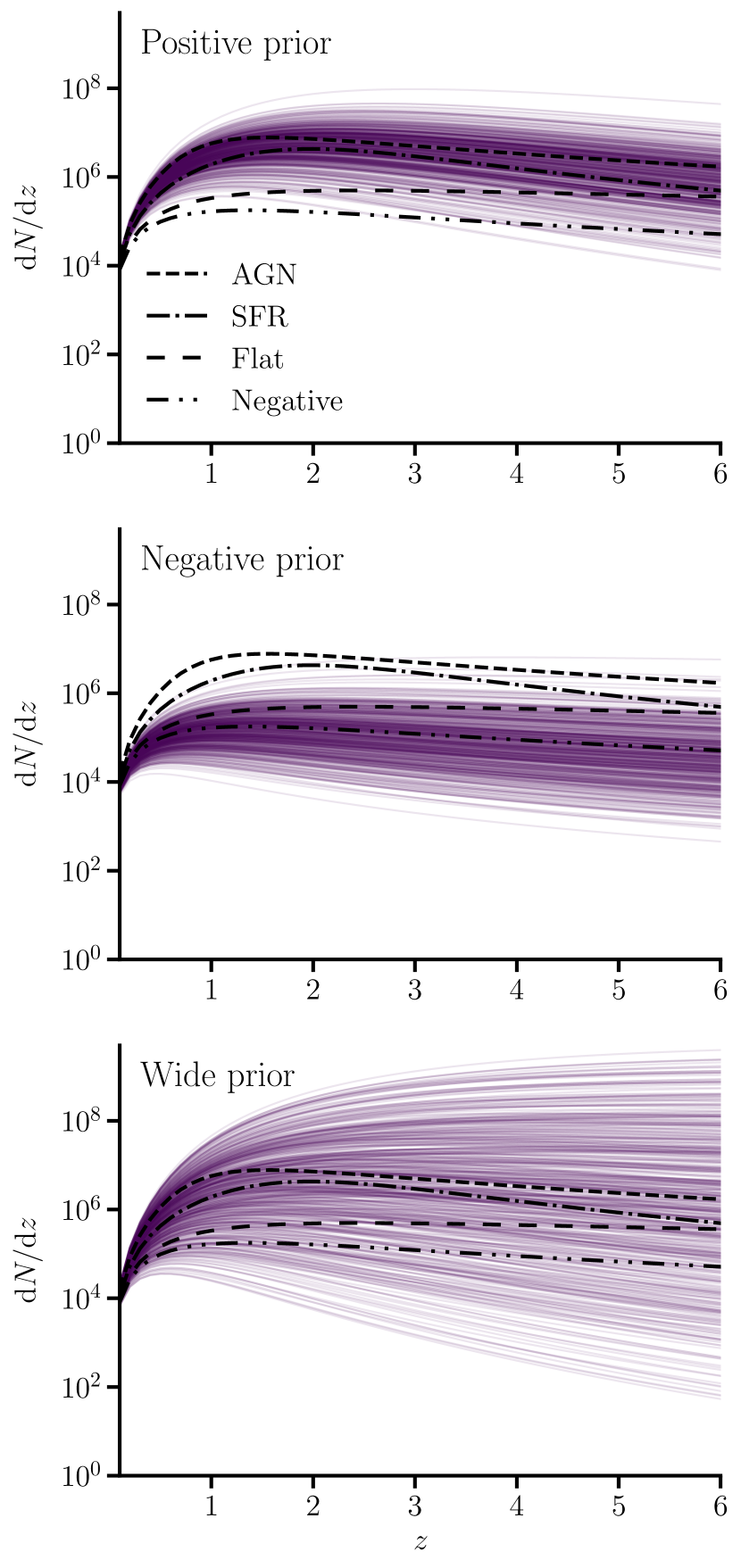
where $n_{0}$ is the local source density. The parameters $p_{1}$, $p_{2}$, and $z_{c}$ can be varied to produce a wide range of possible source evolutions, as shown in Figure 1. We refer to these shape parameters collectively as $\theta=\{p_{1},p_{2},z_{c}\}$ in the following sections for the sake of brevity, as they will typically be treated as nuisance parameters and marginalized over. The expected total number of sources in the universe can be found by integrating the product of the density and comoving volume over redshift as

$$\bar{N}_{\mathrm{s}}^{\mathrm{tot}}=\int_{0}^{\infty}\mathop{\mathrm{d}z}\frac{\mathrm{d}\bar{N}_{\mathrm{s}}^{\mathrm{tot}}}{\mathrm{d}V}\frac{\mathrm{d}V}{\mathrm{d}z}.$$ (5)

The differential comoving volume is given by

$$\frac{\mathrm{d}V}{\mathrm{d}z}=\frac{4\pi cD_{L}^{2}(z)}{H_{0}(1+z)^{2}\sqrt{\Omega_{m}(1+z)^{3}+\Omega_{\Lambda}}},$$ (6)

where $z$ is the redshift, $H_{0}$ is the Hubble constant, and $D_{L}$ is the luminosity distance [31]. We assume a flat $\Lambda\mathrm{CDM}$ cosmology throughout this work, with $H_{0}=70\ \mathrm{km}\ \mathrm{s}^{-1}\ \mathrm{Mpc}^{-1}$, $\Omega_{m}=0.3$, and $\Omega_{\Lambda}=0.7$.

II.3 Incident neutrino flux at Earth

As neutrinos propagate from their sources to Earth, they lose energy due to the adiabatic expansion of the universe such that the arrival energy is related to the emitted energy at the source by a factor of $1+z$. In this way, we can write the differential neutrino flux of a single point source at Earth as

$$\frac{\mathrm{d}\bar{N}_{\nu}^{\mathrm{src}}}{\mathop{\mathrm{d}E}\mathop{\mathrm{d}t}\mathop{\mathrm{d}A}}=Lk_{\gamma}\frac{(1+z)^{2-\gamma}}{4\pi D_{L}^{2}(z)}E_{0}^{-\gamma}\Bigg{(}\frac{E}{E_{0}}\Bigg{)}^{-\gamma},$$ (7)

where the factor of $(1+z)^{2-\gamma}$ is due to the neutrino energy losses. This factor arises as we consider $E_{\mathrm{min}}$ and $E_{\mathrm{max}}$, as defined in Equation (2), to be the energy range within which the luminosity is defined at Earth, not the location of the source. We can define the point source flux normalization, $\phi$, such that

$$\frac{\mathrm{d}\bar{N}_{\nu}^{\mathrm{src}}}{\mathop{\mathrm{d}E}\mathop{\mathrm{d}t}\mathop{\mathrm{d}A}}=\phi\Bigg{(}\frac{E}{E_{0}}\Bigg{)}^{-\gamma},$$ (8)

to simplify this expression. The total differential flux can then be found by integrating over all sources in the population

$$\frac{\mathrm{d}\bar{N}_{\nu}^{\mathrm{tot}}}{\mathop{\mathrm{d}E}\mathop{\mathrm{d}t}\mathop{\mathrm{d}A}\mathop{\mathrm{d}\Omega}}=\frac{1}{4\pi}\int_{0}^{\infty}\mathop{\mathrm{d}z}\frac{\mathrm{d}\bar{N}_{\mathrm{s}}^{\mathrm{tot}}}{\mathrm{d}V}\frac{\mathrm{d}V}{\mathrm{d}z}\frac{\mathrm{d}\bar{N}_{\nu}^{\mathrm{src}}}{\mathop{\mathrm{d}E}\mathop{\mathrm{d}t}\mathop{\mathrm{d}A}}.$$ (9)

Similarly, the total flux of neutrinos between $E_{\mathrm{min}}$ and $E_{\mathrm{max}}$ is given by integrating Equation (7) over energy and then integrating over the source population

$$\frac{\mathrm{d}\bar{N}_{\nu}^{\mathrm{tot}}}{\mathop{\mathrm{d}t}\mathop{\mathrm{d}A}}=\int_{0}^{\infty}\mathop{\mathrm{d}z}\int_{E_{\mathrm{min}}}^{E_{\mathrm{max}}}\mathop{\mathrm{d}E}\frac{\mathrm{d}\bar{N}_{\mathrm{s}}^{\mathrm{tot}}}{\mathrm{d}V}\frac{\mathrm{d}V}{\mathrm{d}z}\frac{\mathrm{d}\bar{N}_{\nu}^{\mathrm{src}}}{\mathop{\mathrm{d}E}\mathop{\mathrm{d}t}\mathop{\mathrm{d}A}}.$$ (10)

For typical source evolutions, as discussed above, we expect the majority of the neutrinos at Earth to come from considerable distances ($z\sim 1$–2), as illustrated in Fig. 1.

Figure 1: The parameterization for the source density evolution given in Equation (4) is shown as thin colored lines for a range of different $p_{1}$, $p_{2}$, and $z_{c}$ values in the top panel. Models typically used to represent the evolution are also plotted as dashed and dotted lines, scaled to a local density of 1 for comparison. The central panel shows the differential probability that a neutrino originates at a redshift $z$, given that it contributes to the flux at Earth. This probability is calculated from the total differential flux above $E_{\mathrm{min}}$, found by evaluating the integrand of Equation (10) for the example case of $n_{0}=10^{-6}$ $\mathrm{Mpc}^{-3}$, $L=10^{42}$ erg $\mathrm{s}^{-1}$, $E_{\mathrm{min}}=E_{0}=100$ TeV, $E_{\mathrm{max}}=\infty$ and $\gamma=2$. The bottom panel shows the corresponding cumulative probability. The AGN luminosity evolution is taken from the best-fit pure luminosity evolution (PLE) model in Ueda et al. [30], and the SFR evolution is as presented in Equation (15) of Madau and Dickinson [23]. Flat signifies no evolution and negative is $\propto(1+z)^{-1}$.

III Neutrino detection with IceCube

Neutrinos are detected through their interactions in dense, transparent media, typically ice or water. In principle, the approach described in this work can be applied to any neutrino detector, but here we will focus on the case of the IceCube neutrino observatory, given that it is currently the only instrument to have detected an astrophysical flux of neutrinos.

The IceCube detector is essentially a cubic-kilometer of ice at the geographic South Pole that has been instrumented with photomultiplier detector modules. These modules are installed through a grid of strings lowered into the ice at regular intervals between depths of 1450 m and 2450 m. Neutrino interactions produce relativistic secondary particles, which in turn lead to Cherenkov radiation in the ice. These signals are detected in optical wavelengths by the photomultiplier modules and are used to identify neutrino-induced events and reconstruct the direction and energy of these incoming neutrinos. A detailed description of the IceCube instrumentation can be found in Achterberg et al. [32], Aartsen et al. [33].

Due to the geometry of the Earth, the energy-dependence of the neutrino interaction cross-section, and the details of the detection process, any neutrino detector will have an effective area that is both a function of the neutrino arrival energy and direction, $A_{\mathrm{eff}}(E,\omega)$. As IceCube is located at the South Pole, its effective area is independent of right ascension and purely a function of declination, $\delta$. The expected number of detected neutrinos from a single source can be found by convolving its flux with the effective area of the detector and integrating over the exposure time

$$\bar{N}_{\nu}^{\mathrm{src}}=T\int_{E_{\mathrm{min}}}^{E_{\mathrm{max}}}\mathop{\mathrm{d}E}A_{\mathrm{eff}}(E,\delta)\frac{\mathrm{d}\bar{N}_{\nu}^{\mathrm{src}}}{\mathop{\mathrm{d}E}\mathop{\mathrm{d}t}\mathop{\mathrm{d}A}},$$ (11)

where $T$ is the total observation time. For each event, the photomultiplier signals are reconstructed to estimate the neutrino energy and direction. In this way, a resulting dataset is a number of neutrino events, their reconstructed energies, $\hat{E}$, arrival directions, $\hat{\omega}$, and the corresponding uncertainties on these measurements. This information can be used to separate neutrino-induced events from other background signals. However, it is more difficult to differentiate between astrophysical neutrinos and atmospheric neutrinos due to cosmic ray interactions in the Earth’s atmosphere. The origin of a neutrino event can only be determined in a probabilistic way, with the measured neutrino energy as the driving factor.

There are two main event types in a neutrino detector like IceCube: “tracks” from muons produced in charged-current interactions of muon neutrinos, and “cascades” from charged-current interactions of electron and tau neutrinos, as well as neutral-current interactions of all flavors [34]. In this work, we rely on results from the analysis of up-going muon tracks from the Northern sky, produced by muon neutrinos interacting both within and outside of the instrumented volume. In this case, the effective area of the detector is much larger in comparison with “cascade”-like neutrino interactions that must occur within the sensitive volume in order to be identified. Due to their topology, track events have a better angular resolution of $\sim 0.5^{\circ}$ at the highest energies, making them more sensitive to the detection of point sources via the method described in Section IV. However, only the energy of the resulting muon is sampled in the detector, so $\hat{E}$ is a lower limit on the reconstructed muon energy and the energy resolution is much worse than for cascade events. The geometry of the Earth and the location of IceCube at the South Pole mean that events coming from the Northern hemisphere have a lower background, due to the absorption of atmospheric muons produced in cosmic ray-induced air showers. The combination of these factors makes the Northern sky muon track sample the most sensitive to point-like neutrino sources, and therefore it provides the most substantial constraints on the source population in our model.

Due to neutrino oscillations, we expect the flavor composition of the neutrino signal to be equally partitioned at Earth for standard extra-Galactic source scenarios [35, 36]. As our analysis is based on a muon track sample, we consider the per-flavor flux summed over muon neutrinos and muon anti-neutrinos throughout this work.

IV Individual source detection probability

To understand the implications of a non-detection of sources for our population model, it is essential to define the criteria required for detection. Previous work in this area has considered the observation of neutrino multiplets as a sufficient requirement, where a multiplet is defined as two or more high energy ($\hat{E}>100$–200 TeV) neutrino events that come from similar directions [15, 18, 19, 20, 21]. While the highest energy neutrinos are the most likely to be astrophysical and have the best angular resolution, the atmospheric background is not negligible at these energies, with some events having a probability of astrophysical origin in the range of 0.5 to 0.7 [6]. Additionally, we do not know a priori whether two neutrinos originate from the same source. The angular resolution at these energies is around $0.5^{\circ}$, but the overlap of two error regions would not be sufficient to report a detection due to the probability of this occurring by chance, which becomes increasingly non-negligible as IceCube continues to gather data.

It is possible to introduce a correction factor for the number of false multiplets in this approach, as shown in [20], but this implies reducing the constraining power of the analysis. We also note that in the existing 3-year public dataset [37], there are now several multiplets above 50 TeV, so this criterion has been surpassed with no reported source detections. In general, the number of multiplets is expected to increase as more data is acquired. To continue to use the multiplet approach to define the non-detection of point sources by IceCube, it is necessary to either increase the energy threshold or to change the definition to require three or more events to have consistent directions, again weakening the subsequent constraints on the properties of the source population.

In this work, we go beyond the assumption of neutrino multiplets corresponding to a source detection. The IceCube Collaboration has developed methods for the detection of neutrino sources that are optimized in terms of their sensitivity to background-dominated signals. The standard point source search method makes use of the reconstructed energies and arrival directions of neutrinos with a likelihood ratio technique for the comparison of source and background hypotheses, as described in Braun et al. [38]. In order to include all relevant information into the likelihood and maximize the discovery potential, these searches also make use of lower energy events in the sample down to $\sim 100$ GeV. As a consequence, the IceCube point source search is more sensitive to source detection than solely considering high-energy events. A more sensitive detection criterion implies more stringent constraints on the source population for a non-detection, and is therefore a favorable starting point for this analysis. The point source search also has the benefit of consistently accounting for statistical fluctuations and the presence of the atmospheric neutrino background. We briefly describe the IceCube point source search methodology in Section IV.1, then explain how we can use this analysis to define the detection probability in Section IV.2.

IV.1 The IceCube point source search

The unbinned likelihood ratio method used by the IceCube Collaboration is based on the likelihood function for the reconstructed neutrino energies and arrival directions at a general, test source point on the sky, $\omega_{s}=(\alpha_{s},\delta_{s})$. The likelihood is essentially a mixture model over the possible source and background contributions with the form

$$\mathcal{L}(\omega_{s},\bar{N}_{\nu}^{\mathrm{src}},\gamma)=\prod_{i=1}^{N_{\nu}}\Bigg{[}\frac{\bar{N}_{\nu}^{\mathrm{src}}}{N_{\nu}}S_{i}(\omega_{s},\gamma)+\bigg{(}1-\frac{\bar{N}_{\nu}^{\mathrm{src}}}{N_{\nu}}\bigg{)}B_{i}\Bigg{]}P(\gamma),$$ (12)

where $N_{\nu}$ is the total number of neutrinos in the sample, $\bar{N}_{\nu}^{\mathrm{src}}$ is the expected number of signal events, and $S_{i}$ and $B_{i}$ are the signal and background likelihoods respectively for the $i^{\mathrm{th}}$ event. There is also an optional prior term, $P(\gamma)$, to include information on the spectral index from analyses of the diffuse flux. The source and background likelihoods factor into independent spatial and energy likelihoods for the event properties

$$S_{i}=P(\hat{\omega}|\omega_{s},\sigma_{i})P(\hat{E}|\gamma),$$ (13)

$$B_{i}=P(\hat{\omega}|\mathrm{BG})P(\hat{E}|\mathrm{BG}),$$ (14)

where $\sigma_{i}$ is the event-by-event uncertainty on the angular reconstruction. In practice, events far from $\omega_{s}$ have a negligible probability of contributing to the likelihood, so a band in declination is selected for a more efficient analysis. In this case, $N_{\nu}$ is the total number of events in the band, and the background spatial likelihood for isotropic emission is a function of the declination-dependence of the atmospheric neutrino background in the band [39].

A set of $\omega_{s}$ is then defined to scan over the sky. At each source position, the likelihood is maximized with respect to $\bar{N}_{\nu}^{\mathrm{src}}\geq 0$ and $1\leq\gamma\leq 4$. The best-fit $\hat{N}_{\nu}^{\mathrm{src}}$ and $\hat{\gamma}$ are used in a likelihood ratio test to compare the hypotheses of clustered point source emission and isotropic background. The likelihood ratio test statistic is

$$\lambda=-2\log\Bigg{[}\frac{P(\omega_{s},N_{\nu}^{\mathrm{src}}=0|\hat{\omega},\hat{E})}{P(\omega_{s},\hat{N}_{\nu}^{\mathrm{src}},\hat{\gamma}|\hat{\omega},\hat{E})}\Bigg{]}.$$ (15)

To understand the performance of the analysis and the significance of the results, the distribution of $\lambda$ is profiled through Monte Carlo simulations for the case of purely background events. The $\lambda$ corresponding to the $5\sigma$ tail probability, $\lambda_{5\sigma}$, can then be defined, which is typically between 20 and 30. By simulating the $\lambda$ distribution in the case of injected source events, it is also possible to define the “discovery potential,” $\phi_{\mathrm{dp}}$, as the point source flux which leads to $>5\sigma$ deviation from background for 50% of repeated simulated trials, given $\omega_{s}$ and $\gamma$. As a scan of point source searches is carried out at different locations over the sky, a source found to have a local significance of $5\sigma$ would then have a trial factor correction applied to calculate the final p-value relevant for a discovery announcement. This is estimated in various ways from simulated experiments, and typically has a value of $\sim 10^{5}$, such that a source with a pre-trial p-value of $10^{-7}$ would have a post-trial p-value of only $10^{-2}$.

IV.2 Defining the detection probability

We can make use of the IceCube point source search framework in order to quantify source detection. We define the requirement for the detection of a neutrino point source as $\lambda>\lambda_{5\sigma}$. While this is not the criterion that would be used to announce a discovery due to the lack of a trial factor correction, it is the most constraining criterion that can be used to connect with the current results of the IceCube point source searches. In this way, the detection probability of a source will depend on its flux, its spectral index, and its location on the sky in relation to IceCube’s effective area and so have the form

$$P_{\mathrm{det}}=P(\mathrm{det}|\phi,\gamma,\delta),$$ (16)

where we have used the fact that IceCube’s effective area is independent of right ascension and used the notation for the point source flux introduced in Equation (8).

The IceCube point source analyses usually report $\phi_{\mathrm{dp}}$ as a function of declination for specific spectral indices, e.g., Fig. 3 and Fig. 18 in Aartsen et al. [9], as well as Fig. 2 here. These plots directly give the source parameters corresponding to $P_{\mathrm{det}}=0.5$. However, to fully characterize how the detection probability depends on the source parameters, we use simulations to profile the $\lambda$ distribution for a range of relevant source positions and properties. In our simulations, we make use of the publicly available information regarding the IceCube effective area to muon track events from Aartsen et al. [37] to calculate the total number of neutrinos for a given flux. We also use the angular resolution information reported in Aartsen et al. [37] to model the distribution of the reconstructed arrival direction $\hat{\omega}$, and the correspondence between reconstructed muon energy and true neutrino energy reported in Aartsen et al. [40] to estimate the energy resolution and model the distribution of the reconstructed energy $\hat{E}$. We approximate the atmospheric neutrino spectrum as a broken power law, and the astrophysical spectrum is modeled with a single power law. To evaluate the discovery potential, we combine our simulated datasets with the procedure outlined in Section IV.1. We verify the ability of this approach to recreate the reported discovery potential plots from existing IceCube publications, showing our results in Appendix B.

Figure 2: The discovery potential calculated using the method described in Section IV.1 applied to simulated data in order to reproduce the discovery potential presented in Fig. 18 of Aartsen et al. [9], which are shown for comparison. The flux is shown normalized to $E_{0}=100$ TeV.

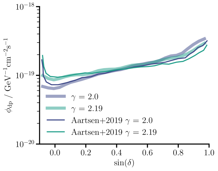
We then implement our approach to reproduce the sensitivity of the analysis described in Aartsen et al. [9]. To do this, we follow their analysis by simulating 497,000 events to reflect eight years of data, and incorporating the results of Aartsen et al. [6] and Haack and Wiebusch [41] by modeling a diffuse astrophysical background as well as the atmospheric component. We also include a prior on the spectral index. Due to the improved discovery potential of including lower energy events into the analysis, we follow the approach of IceCube and assume that sources have a power-law neutrino spectrum that extends to energies as low as $E_{\mathrm{min}}^{\mathrm{PS}}=1$ TeV and up to $E_{\mathrm{max}}^{\mathrm{PS}}=100$ PeV when calculating the detection probability used in this work. The minimum energy is slightly higher than the lowest energies considered for the sample used in Aartsen et al. [9] (see Table 1 therein) as it was not possible to estimate the energy resolution of the detector well below 1 TeV using the publicly available information reported in Aartsen et al. [40]. However, the impact of this on the presented detection probability is negligible given the small effective area of IceCube below 1 TeV and the relative contribution of the lowest energy events in the sample to the point source likelihood function described in Equation (12). Taking these factors into account, we can reasonably reproduce the discovery potential as a function of declination, as shown in Fig. 2. The overall shape is well reproduced for the different spectral indices, but we see that at higher $\sin(\delta)$, the discovery potential is slightly overestimated. This is likely due to the approximate treatment of the effective area and instrument response that we have used in our simulations, based on publicly available information. In contrast, the IceCube Collaboration analyses make use of much more lower-level information and detailed simulations. In any case, the impact of overestimating the discovery potential at this level is negligible on the final results.

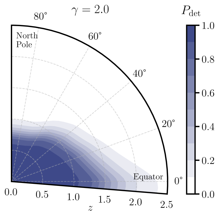
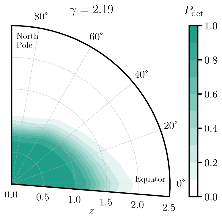
Having verified this method, we can then use it to calculate $P(\mathrm{det|\phi,\gamma,\delta})$ for a range of source parameters, as shown in Fig. 3. We see that for harder spectral indices, the detection probability is highly declination dependent. This variation is because of the energy dependence of the IceCube effective area, and the importance of high energy neutrinos in discriminating potential sources from the background. At high declinations, the highest energy neutrinos suffer Earth-absorption and are not detected. Conversely, at low declinations, high energy source neutrinos can make a substantial contribution to the signal. For this reason, a source producing a constant number of neutrinos above a certain energy can be detected from higher redshift if it has a harder spectral index and is located at lower declinations.

Figure 3: The detection probability is shown as a function of redshift (radial axis), declination (angular axis), and spectral index (upper and lower panels). The weight of the colored segments shows the detection probability from 0 to 1, as indicated by the color bars. For simplicity, we show ten detection probability bins and two spectral indices. In practice, we can compute these values with finer resolution, as required. In both panels, the detection probability is calculated for a source with a constant emission rate above 100 TeV of $\mathrm{d}N_{\nu}/\mathrm{d}t=10^{44}$ $\mathrm{s}^{-1}$ to facilitate comparison. Here, 100 TeV is chosen as an example and the actual calculation of the detection probability includes neutrinos with energies down to 1 TeV, as detailed in the text. At high declinations, the results are extrapolated from $\sin(\delta)=0.97$ to avoid boundary effects.

The detection probability can be included in the physical picture described in Section II by defining the expected number of detected sources in a given population as

$$\bar{N}_{\mathrm{s}}=\frac{1}{2}\int_{\delta_{\mathrm{min}}}^{\pi/2}\mathop{\mathrm{d}\delta}\cos\delta\int_{0}^{\infty}\mathop{\mathrm{d}z}P(\mathrm{det}|\phi,\gamma,\delta)\frac{\mathrm{d}\bar{N}_{\mathrm{s}}^{\mathrm{tot}}}{\mathrm{d}V}\frac{\mathrm{d}V}{\mathrm{d}z},$$ (17)

where $\delta_{\mathrm{min}}\simeq-5^{\circ}$ is the minimum declination used in the search for sources, given that we focus on Northern sky searches, and we note that $\phi$ is a function of $z$, as shown in Equations (7) and (8).

IV.3 Limitations of this approach

The IceCube approach to defining the discovery potential implicitly relies on inevitable stopping and testing intentions that must be defined when calculating p-values [42]. This strategy means that a set number of neutrinos are used in the background and injected source simulations, reflecting the observed number of neutrinos in the point source analysis dataset. This procedure connects the individual source detection probability to the higher-level population parameters through the source flux, $\phi(L,z)$, and spectral index, $\gamma$. However, we also need to account for the effect of varying $n_{0}$ and $\theta$. Changing the source density and evolution will lead to different diffuse astrophysical neutrino backgrounds, and therefore different background $\lambda$ profiles and associated $\lambda_{5\sigma}$ levels. In this way, the full detection probability has the form

$$P_{\mathrm{det}}=P(\mathrm{det}|\phi,\gamma,\delta,n_{0},\theta).$$ (18)

Calculating the detection probability as a function of these parameters is very computationally expensive, as noted in Section 5 of Aartsen et al. [9], in which this has been done for fixed values of $\gamma$ and $\theta$. Additionally, as the diffuse background to point source detection is dominated by the atmospheric component, we do not expect a significant impact of this effect on the results, as quantified in Appendix C. For this reason, we use the implementation of the detection probability described in Equation (16) in this work.

V Statistical formalism

The physical model presented in Section II and the detector description given in Section III connect the high-level population parameters to the detected neutrinos and their properties. This dataset can then be used to reconstruct the observed astrophysical flux and to search for individual sources, as detailed in Section IV. In order to use this connection to place constraints on the nature of the sources, we need to derive a likelihood function for these observations, given the model assumptions and parameters. The case of observations of a population of similar sources is particularly well-suited to a statistical framework known as hierarchical or multi-level modeling [43], where the individual sources share certain properties. We use a Bayesian approach to infer the allowed regions of parameters through the computation of the posterior distribution, under the assumptions of our model and the observations.

Ideally, the likelihood function would be derived for the lowest level available data, the individual neutrino energies, and arrival directions. However, given the computational complexity of this implementation and the limited publicly available information, we choose to take a more practical approach that makes use of existing IceCube results. We first introduce the observable quantities used in Section V.1 and then make use of the hierarchical modeling approach to construct the likelihood function in Section V.2, along with a discussion of the parameter priors chosen. The computational implementation of this likelihood in order to perform inference is described in Section V.3.

V.1 Reconstructed quantities

The IceCube collaboration measures the flux of astrophysical neutrinos using a maximum likelihood analysis based on the reconstructed event energies and arrival directions. The astrophysical neutrino spectrum is typically reported in the form

$$\frac{\mathrm{d}N_{\nu}^{\mathrm{tot}}}{\mathop{\mathrm{d}E}\mathop{\mathrm{d}t}\mathop{\mathrm{d}A}\mathop{\mathrm{d}\Omega}}=(\hat{\Phi}\pm\sigma_{\Phi})\Bigg{(}\frac{E}{E_{0}}\Bigg{)}^{-(\hat{\gamma}\pm\sigma_{\gamma})},$$ (19)

where $E_{0}$ is 100 TeV, and $\hat{\Phi}$ is the estimated differential flux normalization at $E_{0}$. The uncertainties on the reconstructed flux and spectral index are given by $\sigma_{\Phi}$ and $\sigma_{\gamma}$, respectively. These represent the 68% confidence intervals based on the profile likelihood using Wilk’s theorem [44] and include both statistical and systematic uncertainties. Using the physical model described in Section II, we can express the total differential flux at Earth by integrating over the contribution due to all sources in the population, as shown in Equation (9).

The detection probability of a single source is defined in Section IV. Equation (17) represents the number of sources that we would expect to detect from a population, given the population parameters and the IceCube sensitivity of the point source analysis. The non-observation of point sources in this framework can be summarized by $N_{\mathrm{s}}=0$ given $P(\mathrm{det}|\phi,\gamma,\delta)$, where $N_{\mathrm{s}}$ is the detected number of sources. This result can then be used to quantify the implications for the population model.

V.2 Hierarchical model

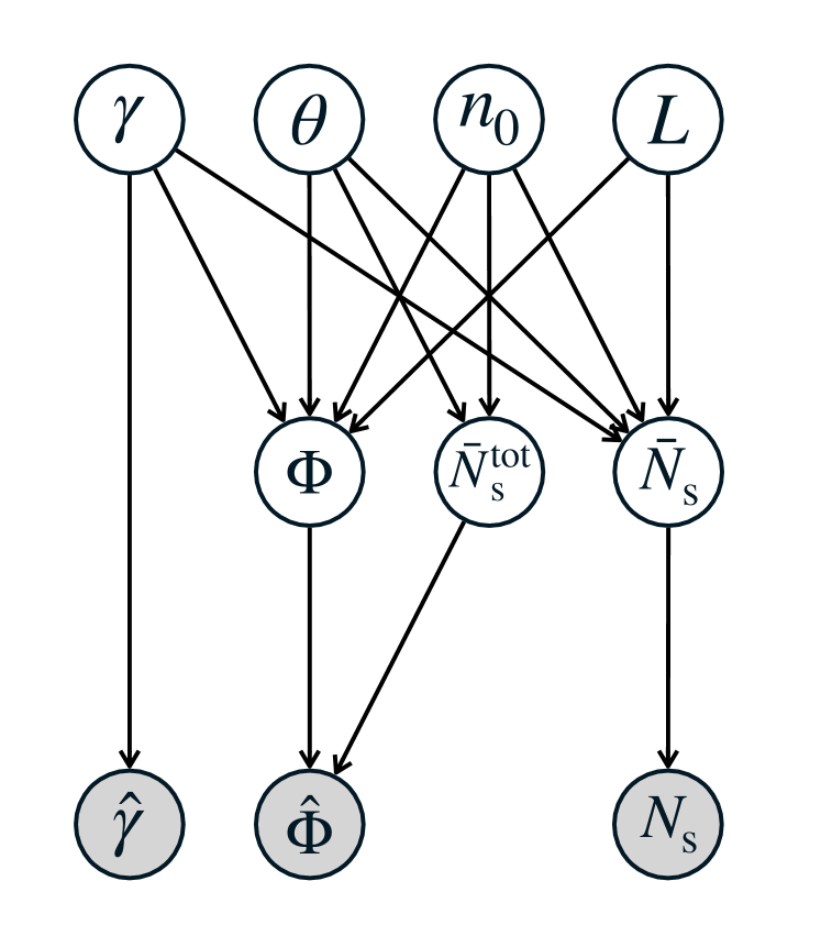
We derive an expression for the unnormalized posterior distribution through a hierarchical modeling approach. The idea is to connect the constraints on the model parameters by requiring our population model to explain both the diffuse flux observations and the non-detection of point sources. The structure of the likelihood is shown diagrammatically in Fig. 4. This figure can be understood as a representation of the generative model needed to produce the IceCube observations. If we were to simulate these observations, we would start by defining the top-level parameters, use these to derive the lower level or “latent” parameters, and finally sample the observations based on the values of these latent parameters. Writing down the generative model for the observations gives us all the ingredients needed to derive the likelihood function. The full derivation for the posterior distribution is given in Appendix D. Here, we use Fig. 4 to intuitively state the connections between observations and parameters and then discuss the form of the resulting expressions. The model parameters are summarized in Table 1 for reference.

Parameters
$\gamma$	Spectral index
$\theta$	Population evolution shape $\{p_{1},p_{2},z_{c}\}$
$n_{0}$	Local source density
$L$	Observed muon neutrino luminosity
$\Phi$	Diffuse flux normalization
$\bar{N}_{\mathrm{s}}^{\mathrm{tot}}$	Expected number of sources in the universe
$\bar{N}_{\mathrm{s}}$	Expected number of detected sources
Observables
$\hat{\gamma}$	Reconstructed $\gamma$
$\hat{\Phi}$	Reconstructed $\Phi$
$N_{\mathrm{s}}$	Number of detected sources

Table 1: Summary of model parameters and observables. The luminosity is defined between $E_{\mathrm{min}}^{L}=10$ TeV and $E_{\mathrm{max}}^{L}=10$ PeV and the diffuse flux normalisation is also at $E_{0}=100$ TeV.

Starting at the top of Fig. 4, the high-level parameters or hyperparameters are assumed to be independent. To include knowledge on our modeling assumptions and avoid giving weight to unphysical regions of the parameter space, weakly informative prior distributions [43, 45] are placed on the high-level parameters, with $n_{0}$ and $L$ described by broad lognormal distributions to reflect our uncertainty, and bounded to sensible values. The evolution parameters, $\theta$, can either be left free to cover a range of plausible source evolutions or more constrained to follow positive or negative evolution models, as shown in Fig. 5. We summarize the high-level parameters and their priors in Table 2. In both Fig. 5 and Table 2, we refer to the priors on $\theta$ as “positive”, “negative” and “wide”, where the first two terms reflect the source evolution models conisdered and the latter reflects the choice of a wide range of possible evolutions. Stepping down one level in Fig. 4, we have the latent parameters, $\Phi$, $\bar{N}_{\mathrm{s}}^{\mathrm{tot}}$, and $\bar{N}_{\mathrm{s}}$. These latent quantities can all be directly calculated from the high-level model parameters, as described by Equations (9), (5), and (17), respectively.

Finally, the likelihood for the observations is given by

$$P(\hat{\gamma},\hat{\Phi},N_{\mathrm{s}}|\bar{N}_{\mathrm{s}},\bar{N}_{\mathrm{s}}^{\mathrm{tot}},\Phi)=P(\hat{\gamma}|\gamma)P(\hat{\Phi}|\bar{N}_{\mathrm{s}}^{\mathrm{tot}},\Phi)P(N_{\mathrm{s}}|\bar{N}_{\mathrm{s}}),$$ (20)

where the conditional terms connect the high-level parameters to the observations through the latent parameters. $P(\hat{\gamma}|\gamma)$ is approximated by a normal distribution with mean $\gamma$ and standard deviation $\sigma_{\gamma}$. Similarly, $P(N_{\mathrm{s}}|\bar{N}_{\mathrm{s}})$ is given by a Poisson distribution with mean $\bar{N}_{\mathrm{s}}$. In the high $n_{0}$ limit, the final term $P(\hat{\Phi}|\bar{N}_{\mathrm{s}}^{\mathrm{tot}},\Phi)$ is effectively independent of $\bar{N}_{\mathrm{s}}^{\mathrm{tot}}$ and lognormal. However, in the low $n_{0}$ limit, the observed astrophysical flux depends on the presence of sources in the observable universe, and a universe with no sources is incompatible with the observation of an astrophysical flux. We can encode this by expanding this term as a mixture model over the two relevant cases

$$\begin{split}P(\hat{\Phi}|\bar{N}_{\mathrm{s}}^{\mathrm{tot}},\Phi)=&\ P(N_{\mathrm{s}}^{\mathrm{tot}}=0|\bar{N}_{\mathrm{s}}^{\mathrm{tot}})P(\hat{\Phi}|N_{\mathrm{s}}^{\mathrm{tot}}=0)\\ &+P(N_{\mathrm{s}}^{\mathrm{tot}}\neq 0|\bar{N}_{\mathrm{s}}^{\mathrm{tot}})P(\hat{\Phi}|\Phi).\end{split}$$ (21)

where the first term in the mixture is the Poisson probability of observing $N_{\mathrm{s}}^{\mathrm{tot}}=0$, given $\bar{N}_{\mathrm{s}}^{\mathrm{tot}}$, multiplied by a lognormal distribution for $\hat{\Phi}$, centered on an effectively zero flux with standard deviation $\sigma_{\Phi}$. Similarly, the second term is weighted by the Poisson probability that $N_{\mathrm{s}}^{\mathrm{tot}}\neq 0$ multiplied by a lognormal distribution with mean $\Phi$ and standard deviation $\sigma_{\Phi}$.

Figure 4: Directed acyclic graph showing the hierarchical likelihood function given in Equation (20). The unshaded circles show the free parameters, and the shaded circles represent observed quantities, with the arrows showing the connections between them. The parameters are described in the text.

	Prior	Lower	Upper	Unit
$n_{0}$	$\mathrm{Log\mathcal{N}}(\log(10^{-6}),30)$	$10^{-12}$	$10^{2}$	Mpc-3
$L$	$\mathrm{Log\mathcal{N}}(\log(10^{42}),30)$	$10^{35}$	$10^{50}$	TeV s-1
$\gamma$	$\mathcal{N}(2,3)$	1	4	-
$\theta$ – positive
$p_{1}$	$\mathcal{N}(19.3,0.2)$	18.1	20.5	-
$p_{2}$	$\mathcal{N}(24.9,0.2)$	23.7	26.1	-
$z_{c}$	$\mathcal{N}(1.76,0.12)$	1.04	2.48	-
$\theta$ – negative
$p_{1}$	$\mathcal{N}(19.3,0.2)$	18.1	20.5	-
$p_{2}$	$\mathcal{N}(20.5,0.2)$	19.3	21.7	-
$z_{c}$	$\mathcal{N}(1.0,0.08)$	0.52	1.48	-
$\theta$ – wide
$p_{1}$	$\mathcal{U}(19,21)$	19	21	-
$p_{2}-p_{1}$	$\mathcal{U}(0,6)$	0	6	-
$z_{c}$	$\mathcal{U}(1.0,1.8)$	1.0	1.8	-
$M$	Represents other prior assumptions related to the choice of the physical model.

Table 2: Prior choices for the high-level model parameters. The columns labeled “Lower” and “Upper” given the lower and upper bounds placed on parameters. The three different cases for the source evolution parameters, $\theta$, correspond to the three different panels in Fig. 5. We also introduce $M$ to encode the implicit conditioning of our results on the choice of an astrophysical source population made up of discrete sources with power-law spectra and shared luminosities. The notation $\mathrm{Log}\mathcal{N}$(mean, standard deviation), $\mathcal{N}$(mean, standard deviation) and $\mathcal{U}$(lower bound, upper bound) is used to summarize the lognormal, normal and uniform distributions, repectively.

Figure 5: The source redshift distribution is shown for the three different priors on the source evolution parameters, $\theta=\{p_{1},p_{2},z_{c}\}$, as presented in Table 2. The top panel shows the case where the prior on $\theta$ is chosen to reflect a positively evolving source distribution, similar to that of the SFR or AGN luminosity function, the middle panel shows a flat or negative evolution, and the bottom panel shows a relatively unconstrained evolution model. In each case, 500 random draws from the prior are shown, so the density of curves reflects the weight of the prior probability. Typical source evolution choices are shown for comparison, as in Fig. 1.

V.3 Inference

For a given set of observations, we infer the model parameters using Bayesian inference. Bringing together the likelihood function from Equation (20) and the priors described in Table 2, the joint posterior distribution for the model parameters, given the observations is

$$\begin{split}P(\theta,n_{0},\gamma&,\bar{N}_{\mathrm{s}},\bar{N}_{\mathrm{s}}^{\mathrm{tot}},\Phi|N_{\mathrm{s}},\hat{\Phi},\hat{\gamma},M)\\ \propto&~{}P(\theta,n_{0},L,\gamma|M)P(\bar{N}_{\mathrm{s}}|\theta,n_{0},L,\gamma)\\ &\times P(\bar{N}_{\mathrm{s}}^{\mathrm{tot}}|n_{0},\theta)P(\Phi|\theta,n_{0},L,\gamma)\\ &\times P(\hat{\gamma}|\gamma)P(N_{\mathrm{s}}|\bar{N}_{\mathrm{s}})P(\hat{\Phi}|\bar{N}_{\mathrm{s}}^{\mathrm{tot}},\Phi).\end{split}$$ (22)

The full derivation of this expression for the posterior distribution is given in Appendix D. We compute the posterior distribution numerically by drawing samples from it using Stan [46]. This procedure allows us to easily marginalize over the source evolution parameters, the spectral index, and the latent parameters of the model to produce the results shown in Section VII. Stan is an open-source framework for statistical computation with an interface to several different techniques. In particular, we make use of Stan’s adaptive Hamiltonian Monte Carlo [47]. To assess the convergence of the resulting chains to the target distribution, we employ a set of diagnostics implemented within the Stan framework. We require that all chains are sampled with no divergent transitions. Also, for each parameter, we ensure that we have a large effective sample size, $n_{\mathrm{eff}}>1000$ and that the Gelman-Rubin statistic is bounded, $\hat{R}<1.1$, in order to monitor the mixing between chains.

Equations (9) and (17) contain integrals over $z$ from 0 to $\infty$. In practice, we integrate up to some finite $z_{\mathrm{max}}$ to describe the whole Universe, as sources beyond a redshift of $\sim 6$ are expected to have a negligible contribution to the flux at Earth for typical source evolutions, as illustrated in Fig. 1. We verify that the results are not sensitive to the choice of $z_{\mathrm{max}}$. We include the detection probability by fitting a sigmoid over $\phi$ and then tabulating the parameters of the sigmoid over $\gamma$ and $\delta$. These values are then interpolated over in the model in the calculation of $\bar{N}_{\mathrm{s}}$.

VI Application to IceCube observations

We apply the statistical formalism developed in Section V to infer constraints on the steady-state source population parameters from the combined observation of an astrophysical flux but no individual sources. For the non-observation of point sources, we use the results of the point-like source search presented in Aartsen et al. [9]. These results are implemented as $N_{\mathrm{s}}=0$, given that the detection probability is as defined in Section IV, which is not satisfied by any direction in the all-sky analysis in Aartsen et al. [9] (see e.g., Fig. 5 therein). Aartsen et al. [9] make use of the same muon neutrino sample developed for the diffuse astrophysical flux analysis of Aartsen et al. [6] and Haack and Wiebusch [41], expected to contain between 190 and 2145 astrophysical neutrinos. The 8-year diffuse muon neutrino flux results can be summarized as

$$\hat{\Phi}=1.01\times 10^{-18}\ \mathrm{GeV}^{-1}\mathrm{cm}^{-2}\mathrm{s}^{-1}\mathrm{sr}^{-1}$$

$$\sigma_{\Phi}=0.25\times 10^{-18}\ \mathrm{GeV}^{-1}\mathrm{cm}^{-2}\mathrm{s}^{-1}\mathrm{sr}^{-1}$$

$$\hat{\gamma}=2.19$$

$$\sigma_{\gamma}=0.1,$$

using the notation introduced in Equation (19), where we also defined $E_{0}=100$ TeV. The point source analysis presented in Aartsen et al. [9] is optimized to search for sources with similar spectra to the observed diffuse astrophysical flux, and the discovery potential for the Northern sky is on the level of $\phi_{\mathrm{dp}}\sim 10^{-19}$ $\mathrm{GeV}^{-1}\ \mathrm{cm}^{-2}\ \mathrm{s}^{-1}$ for a flux normalization at $E_{0}=100$ TeV.

These two results for the diffuse spectrum and point source search are based on the same neutrino sample and are therefore particularly well-suited to joint analysis. To reflect this sample, we use $\delta_{\mathrm{min}}=-5^{\circ}$ in our joint model. As explained in Section IV.2, we consider a minimum energy of $E_{\mathrm{min}}^{\mathrm{PS}}=1$ TeV and $E_{\mathrm{max}}^{\mathrm{PS}}=100$ PeV in the derivation of the detection probability from the IceCube point source analysis. When interpreting the results and comparing to previous work in Section VII, we instead use $E_{\mathrm{min}}^{L}=10$ TeV and $E_{\mathrm{max}}^{L}=10$ PeV as the energy range within which the neutrino luminosity is defined, as it is not yet confirmed that the power-law astrophysical flux measured by IceCube extends to other energies, and this choice facilitates comparison with previous work.

The IceCube Collaboration has recently presented an updated point source search using ten years of muon track data [11]. This work extends the analysis to both hemispheres, but the Northern sky remains the strongest in terms of sensitivity due to the reduced background to atmospheric neutrinos. In the Northern sky, the discovery potential of this analysis is comparable to that used here for the case of an $E^{-2}$ spectrum but reduced by $\sim 30$% for sources with a softer $E^{-3}$ spectrum. No point sources are found to have a local significance of $>5\sigma$, although signals of $\sim 4\sigma$ have emerged. Due to the comparable discovery potential and lack of $>5\sigma$ detection, our results are still relevant in light of this recent work.

VII Results

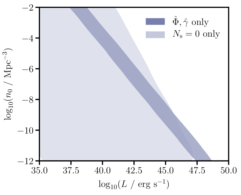
The results can be summarized as the joint posterior distribution over the model parameters. We show the joint and marginal posterior distributions for the high-level population parameters $n_{0}$ and $L$ in Fig. 6. In this way, the two-dimensional joint distribution over $n_{0}$ and $L$ is analogous to the standard presentations of the combined constraints from the observation of a flux, but no point sources, that have been produced in several other publications, including [16, 17, 18, 19, 20, 21]. We see that the current observations disfavor a population of rare, luminous sources, in agreement with what has been found by previous studies of this nature (e.g. [20, 9, 21]). Assuming positive source evolution constrains the population to a narrow region of the parameter space, with $n_{0}\gtrsim 10^{-10}$ $\mathrm{Mpc}^{-3}$ and $L\lesssim 10^{46}$ erg $\mathrm{s}^{-1}$. Flat and negatively evolving populations are more strongly constrained to $n_{0}\gtrsim 10^{-8}$ $\mathrm{Mpc}^{-3}$ and $L\lesssim 5\times 10^{44}$ erg $\mathrm{s}^{-1}$. Considering a more comprehensive range of possible source evolution shapes weakens the constraints, as expected. Denser and less luminous populations are most probable, but the posterior distribution generally has a long tail out to more sparse populations of brighter sources. For illustrative purposes, we also show the constraints on $n_{0}$ and $L$ separately in terms of the flux requirement and non-detection of significant point sources in the right panels of Fig. 6. We see that the joint result is more constraining than the individual contributions. The plots with separate constraints are intended to aid the understanding of the main result and connect to the presentation of results in previous work. We emphasize that in our hierarchical model, the two constraints are coupled through conditional probability statements to the shared high-level parameters, and cannot be treated as independent. Indeed, the posterior distribution is not well-identified in the “$N_{\mathrm{s}}=0$ only” case, and sampling from it can result in divergent transitions.

Figure 6: The joint posterior distribution for $L$ and $n_{0}$ under the observational constraints. The left panels show this distribution under the combined constraints for the case of a positive prior (top), a negative prior (middle) and a more unconstrained prior on $\theta$ (bottom), as detailed in Table 2. The right panels give the same case as the left, with the two observational constraints plotted separately to show their relative contribution to the combined result. The constraint from requiring the source population to reproduce the observed astrophysical flux is labeled “$\hat{\Phi},\hat{\gamma}$ only”, and the constraint from the non-detection of significant point sources is given by “$N_{\mathrm{s}}=0$ only”. For the left plots, the contours show the 30, 60, 90, and 99% highest posterior density credible regions for the joint distributions. In the right plots, only the 99% highest posterior density credible regions are shown. A kernel density estimate is used to plot the posterior samples and calculate the regions of highest posterior density. The non-observation of sources does not constrain low $L$ and large $n_{0}$ values, so the posterior continues unchanged in this regime.

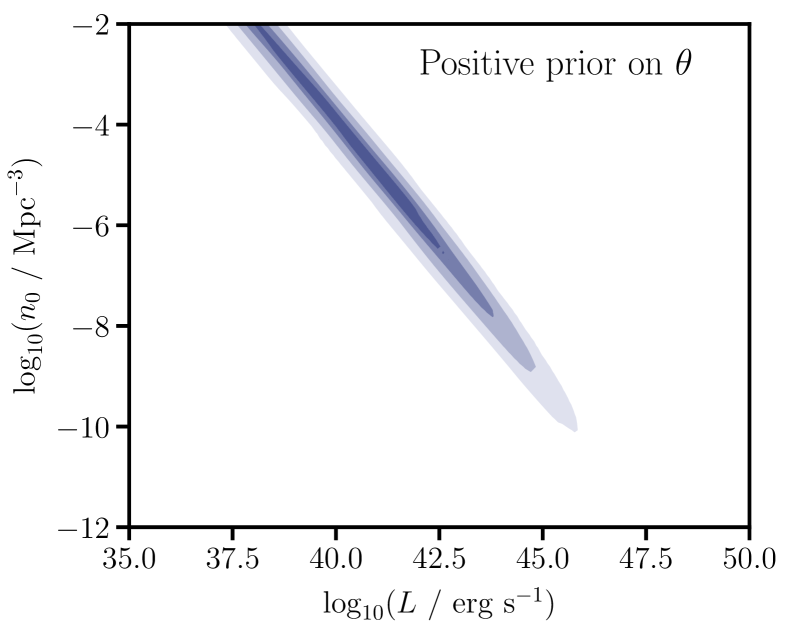
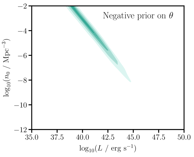
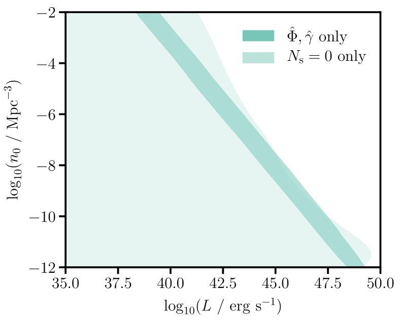
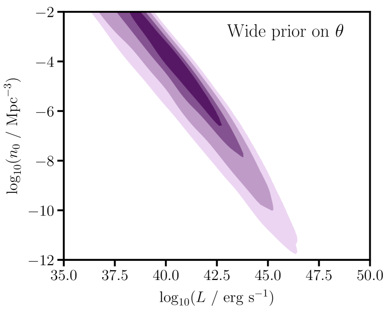
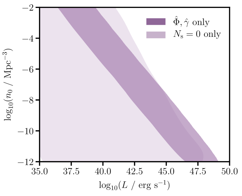
We also show our results in terms of the dependency of the allowed $n_{0}$ values on the source evolution in Fig. 7. Here, we show the same results as in the left panels of Fig. 6, but instead give the joint posterior of $n_{0}$ and $p_{1}-(p_{2}/z_{c})$. $p_{1}$, $p_{2}$ and $z_{c}$ are parameters used to describe the redshift evolution of sources, as introduced in Equation (4). The choice of $p_{1}-(p_{2}/z_{c})$ reflects the behaviour of the evolution at low redshift ($z\ll 1$) and therefore allows us to summarize the $n_{0}$-evolution dependence in a simple 2D plot. We see that the constraints for $n_{0}$ are very much dependent on the evolution model and therefore the different priors chosen. Stronger evolution allows for rarer source populations because in this case the contribution to the observed neutrino flux from nearby sources is relatively small.

Figure 7: The dependence of $n_{0}$ on the source evolution for the three different evolution priors. We show $p_{1}-(p_{2}/z_{c})$ on the x-axis to summarize the dependence of $f(z,\theta)$ from Equation (4) on these parameters at low redshifts ($z\ll 1$). The top panel shows the case of positive and negative evolution models and the bottom panel shows the case for the wide, unconstrained prior. In both panels we also plot the $p_{1}-(p_{2}/z_{c})$ values that correspond to commonly studied evolution models, as introduced in Fig. 1. The contours show the 30, 60, 90 and 99% highest posterior density credible regions, as in the left panels of Fig. 6. It is clear that for more strongly evolving populations (higher values on the x-axis), $n_{0}$ is less constrained.

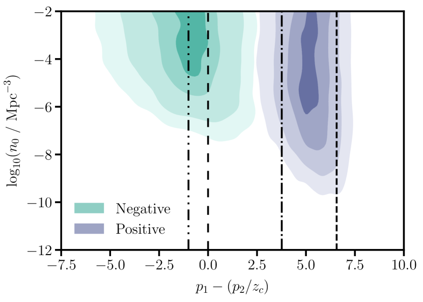
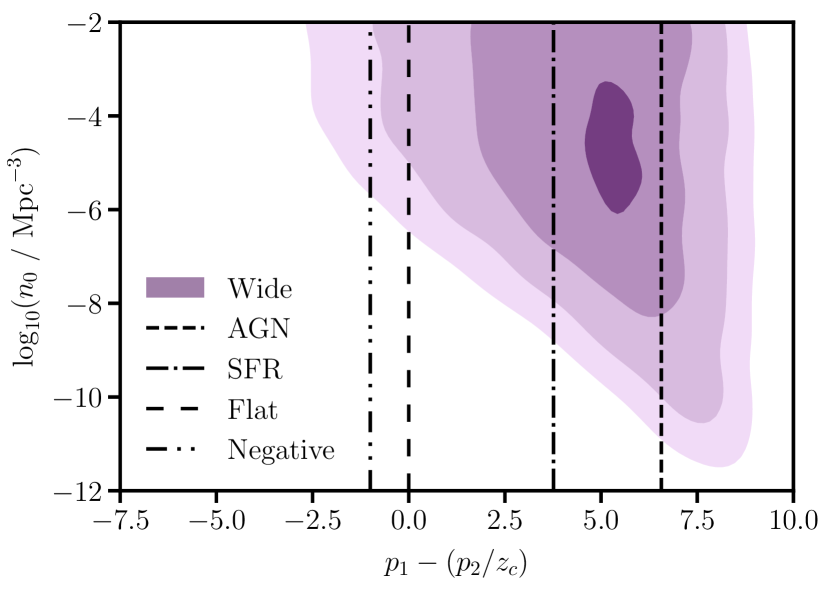
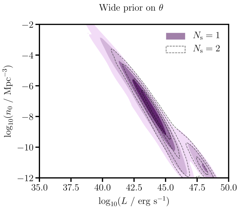
Fig. 6 shows the current source population constraints, assuming the IceCube observation of a flux, non-observation of point sources and the discovery potential described in Section VI. To understand how these constraints would be affected by the possible detection of point sources with the current detector configuration and analysis methods, we also show the results for the counter-factual case of $N_{\mathrm{s}}=1$ and $N_{\mathrm{s}}=2$ in the upper panel of Fig. 8. For this hypothetical example, we consider a population with an unconstrained evolution. The detection of a single point source above the threshold would further constrain the source population to values around $n_{0}\sim 10^{-8}$ $\mathrm{Mpc}^{-3}$ and $L\sim 10^{44}$ erg $\mathrm{s}^{-1}$, with the population shifting to less dense and brighter sources for further point source detections, as can be seen from the shape of the posterior.

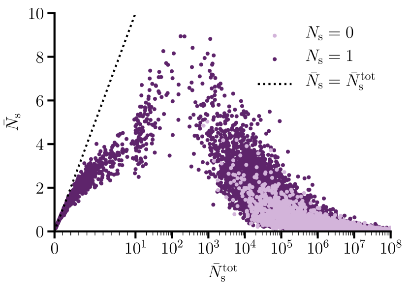
The bimodality in the joint posterior distribution reflects that it is most probable for detected sources to come from a dense population, but there is some non-negligible probability that a few rare, but very bright sources could be responsible for all the observed flux under our assumptions. We illustrate this point further in the lower panel of Fig. 8 by showing the posterior samples of the latent parameters $\bar{N}_{\mathrm{s}}^{\mathrm{tot}}$ and $\bar{N}_{\mathrm{s}}$ for the case of $N_{\mathrm{s}}=1$ (with $N_{\mathrm{s}}=0$ also shown for comparison). Large values of $\bar{N}_{\mathrm{s}}^{\mathrm{tot}}$ directly corresponds to large $n_{0}$, as shown in Equation (5). Therefore, the samples on the right side of this plot reflect the main peak in the upper panel of Fig. 8. As the total number of sources decreases, the energy density implied by the observed flux is shared among fewer sources. As such, each source is brighter, and more sources are detectable. As $\bar{N}_{\mathrm{s}}^{\mathrm{tot}}$ continues to decrease, there are so few sources in the universe that despite their brightness, few are within the $P_{\mathrm{det}}$ horizon, and eventually we reach the regime where $\bar{N}_{\mathrm{s}}=\bar{N}_{\mathrm{s}}^{\mathrm{tot}}$, as marked by the dashed line in the figure. However, this configuration of few total sources is allowed in our model since by considering $N_{\mathrm{s}}>0$, we no longer require the neutrino arrival direction to be close to isotropic. In constrast, for the case of $N_{\mathrm{s}}=0$, we see that only the high-$n_{0}$ component is present, as it would be impossible to have a few bright sources with no source detection. The bimodality arises from requiring that we observe $N_{\mathrm{s}}=1$, which imposes a strong constraint on high $\bar{N}_{\mathrm{s}}$, as shown by the lower density of samples. As this requirement is relaxed and we consider $N_{\mathrm{s}}=2$ and higher, the two peaks move together and eventually merge, as indicated in the upper panel of Fig. 8.

While the second peak around $n_{0}\sim 10^{-11}$ $\mathrm{Mpc}^{-3}$ and $L\sim 10^{48}$ erg $\mathrm{s}^{-1}$ is permitted by these data, it corresponds to the case of $\bar{N}_{\mathrm{s}}^{\mathrm{tot}}<100$, which is not physical for typical source classes considered. Even if one point source were soon detected in IceCube, the overall distribution of astrophysical neutrinos would still be close to isotropic. These anisotropic models are still allowed in our analysis because the observation of an isotropic flux is not explicitly included into the data that we use. To include this information mathematically, it would be necessary to extend the framework described here to incorporate the individual neutrino event arrival directions and energies. We also note that the total observed astrophysical flux is $\sim 10^{-17}$ GeV $\mathrm{cm}^{-2}$ $\mathrm{s}^{-1}$ and the discovery potential used in this work is around $10^{-19}$ GeV $\mathrm{cm}^{-2}$ $\mathrm{s}^{-1}$. So, even if all source fluxes are at the discovery potential, we require at least $4\pi\Phi/\phi_{\mathrm{dp}}\sim 100$ sources to maintain the observed flux and a near-isotropic distribution of detected neutrinos.

Figure 8: The case of an observation of one or two point sources with a pre-trial significance of above 5$\sigma$, with the current sensitivity and observed astrophysical flux. We consider an unconstrained prior on $\theta$ in the calculation of this result. The joint posterior distribution for $L$ and $n_{0}$ is shown in the upper panel, as in Fig. 6. The lower panel shows samples from the joint distribution of the latent parameters $\bar{N}_{\mathrm{s}}^{\mathrm{tot}}$ and $\bar{N}_{\mathrm{s}}$ for the case of $N_{\mathrm{s}}=1$ and $N_{\mathrm{s}}=0$ for comparison. We see that the second peak in the upper panel at low $n_{0}$ and consequently low $\bar{N}_{\mathrm{s}}^{\mathrm{tot}}$ corresponds to the possibility of a few bright sources being responsible for all the observed flux. This model is ruled out by the observation of near-isotropic emission, which is not included in our likelihood, as explained in the text.

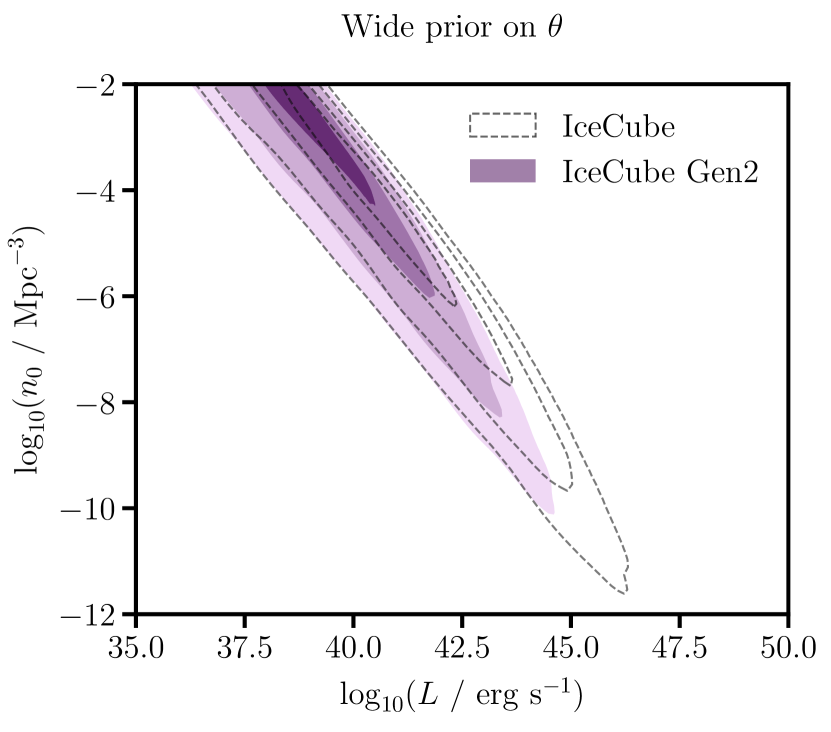
Future detectors will improve the discovery potential of point source analyses. The IceCube Collaboration plans IceCube Gen2, an expansion of the instrumented volume of IceCube from 1 $\mathrm{km}^{2}$ to 10 $\mathrm{km}^{2}$ in the Antarctic ice [48]. The planned design benefits from the increased understanding of the ice properties from the development of IceCube, which makes it possible to dramatically increase the spacing of the strings of photomultiplier detector modules while maintaining the desired performance. By increasing the exposure and angular resolution of the detector (thanks to the longer muon track lengths that can be sampled in a larger volume), there is an expected increase in the discovery potential of a least $\sim 5$ compared to that of the current IceCube results for 15 years of Gen2 operation following 15 years of IceCube [49]. We rescale the detection probability calculated in Section IV.2 by a factor of 5 across all declinations and show the equivalent source population constraints in Fig. 9 for the case of the unconstrained prior on the source evolution parameters. We see that for a continued non-detection of significant individual sources, the constraints become increasingly confined to numerous, dimmer sources, which would produce an unresolvable diffuse flux in the detector. However, due to the uncertainties present, there is still a long tail in the joint distribution out to $n_{0}\sim 10^{-10}$ $\mathrm{Mpc}^{-3}$ and $L\sim 5\times 10^{44}$ erg $\mathrm{s}^{-1}$. The constraints that we find for $n_{0}$ are similar to those reported using an angular power spectrum analysis in Dekker and Ando [50].

The KM3NeT Collaboration is also developing a cubic-kilometer scale neutrino detector in the Mediterranean Sea [51]. The detector is still under construction and has recently started taking data successfully in parallel with its continued expansion. With water as the detection medium, the scattering length of photons in increased, and it is possible to reconstruct the direction of such events with an angular resolution of $<0.2^{\circ}$ at energies of $E>10$ TeV with a similar module spacing to that of IceCube [52]. This high angular resolution means that the KM3Net detector will have an improved discovery potential by a factor of $\sim 3-4$ compared to IceCube’s Northern sky once it reaches its full size and equivalent operation time (see Fig. 9 in Aiello et al. [52]). As the effective area of KM3Net is very different from that of IceCube, in particular in terms of declination dependence, applying our model to this case would require a dedicated study of the detection probability, as described in Section IV. We do not attempt this here, but simply note that the potential impact on the constraints would be somewhere between that of IceCube and IceCube Gen2. The two detectors observe different regions of the sky, and so their operation will be complementary in terms of point source searches.

Figure 9: The joint posterior distribution for $L$ and $n_{0}$ for the case of IceCube Gen2, assuming no point source detections. The results are compared to the IceCube results, considering the case of an unconstrained prior, as shown in the bottom-left panel of Fig. 6. The distributions are plotted as in Fig. 8.

VII.1 Implications

In order to understand the constraints for a particular class of sources, we must model its luminosity distribution, as described in Appendix A. Neutrino luminosity functions are currently unconstrained for all candidate source classes, so it is necessary to assume some connection between the measured electromagnetic emission from a source class and its neutrino emission in the context of a theoretical model. For this reason, we leave such a comparison to future work and highlight the general implications of our results here. A more in-depth discussion of relevant source classes can be found in [18] and [20].

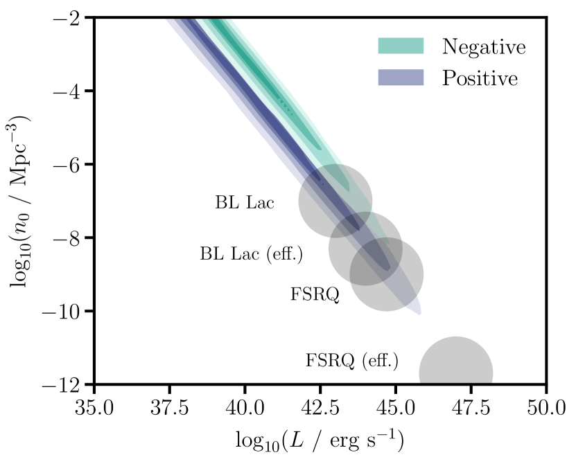
The general implications of our results are that populations of very rare, luminous sources are disfavored as the primary contributors to the observed astrophysical neutrinos, as otherwise, we would have started to detect them as individual sources. This argument can be weakened if we consider non-standard source evolutions, such as for the case of the wide prior on $\theta$ in the bottom-left panel of Fig. 6, and particularly for the case of rapidly evolving sources. For positively evolving source candidates with a local density of $\gtrsim 10^{-6}$ $\mathrm{Mpc}^{-3}$, such as starburst galaxies, AGN and galaxy clusters, the local density is consistent with the 30% region of highest posterior density. At lower densities, possible candidates are energetic blazars such as BL Lac objects. Their evolution is still not clear, with some studies suggesting negative or flat cases (see Ajello et al. 28 and references therein), which provide stronger constraints. Flat-spectrum radio quasars (FSRQs) are popular source candidates with $n_{0}\lesssim 10^{-9}$ $\mathrm{Mpc}^{-3}$ that are widely agreed to have a strong positive evolution. Following the assumptions on the source evolution and luminosity function reported in Ajello et al. [28], we compare the cases for these more constrained sources to our results for positive and negative evolution in Fig. 10. BL Lac objects lie in the tail of our posterior distribution assuming negative evolution, but are still consistent with our results if positively evolving models are considered. FSRQs lie further out, and even including more uncertainty into our model, it is difficult for such a population to explain the IceCube observations without very strong evolution. These results are in general agreement with those found from considering more specific models for the individual source classes [20], but do not disfavour BL Lacs and FSRQs as strongly as previous work. It is important to remember that the $n_{0}$ estimates for these sources depend on the evolution reconstructed from their observations. In this way, further investigation with more model-specific assumptions is necessary for us to draw final conclusions on this matter, and we plan to explore this direction in future work.

Figure 10: The joint posterior distributions are shown for the case of both positive and negative source evolution, as in Fig. 6. We compare these distributions with expected values for BL Lacs and FSRQs that are shown by the shaded circles. These shaded areas are intended to guide the eye to values based on the results presented in Ajello et al. [28]. The label “eff.” denotes an estimate for the local density of these sources that is expected to dominate their contribution to the neutrino flux. This estimate is based on the effective luminosity and the formalism introduced in Murase and Waxman [20]. The specific constraints for BL Lacs and FSRQs depend on the assumptions regarding the source evolution.

We find that the most probable region for the density of the neutrino source population is $n_{0}\geq 10^{-7}$ $\mathrm{Mpc}^{-3}$, which is in general agreement with the results reported in previous work. However, our results show that values down to $n_{0}\sim 10^{-11}$ $\mathrm{Mpc}^{-3}$ are consistent with the current IceCube observations, depending on the source evolution. The tail of the posterior distribution down to lower $n_{0}$ arises as we model the detection probability gradient and include information on uncertainty into our model, as we will discuss further below. Our results are hence less constraining than those reported in Fig. 3 of Murase and Waxman [20], despite making use of the recent IceCube observations and a more constraining detection criterion, as we include more sources of uncertainty. In Murase and Waxman [20], the detection criterion is a multiplet above 50 TeV, including a correction based on the estimated number of atmospheric neutrino events, and the luminosity is defined as the differential energy flux at 100 TeV. We note that there is no major difference in the conclusions reached in our work if the luminosity is redefined in this way. Fig. 4 of Murase and Waxman [20] also shows the case of using harder blazar spectral templates, which is somewhat closer to our results. As we mentioned in Section IV, there are now several multiplets above 50 and even 100 TeV, so the criterion on which these results are based has now been surpassed. Our results are also closer to, but still allow lower $n_{0}$ values than, the SFR case shown in Fig. 4 of Palladino et al. [21], which uses multiplets above 200 TeV as a detection criterion, and Fig. 19 in Aartsen et al. [9], which uses 90% CL upper limits calculated assuming $\gamma=2.19$.

In our work, we have explicitly modeled the detection probability of a statistically significant signal in IceCube instead of assuming that the observation of neutrino multiplets at high energies is a sufficient requirement for detection. We utilize the additional information in lower-energy neutrino events to uncover possible point sources that may not yet result in a high-energy multiplet, making our framework more sensitive. While there are higher backgrounds at lower energies, the power-law nature of the expected source fluxes means that this information is still useful in the statistical detection of sources. Additionally, high-energy events can also appear as low energy tracks that start outside the detector. If we ignore the sources of uncertainty in our model and use the same assumptions applied in previous studies, we actually find results that are more constraining than those reported in Aartsen et al. [9] and Palladino et al. [21]. We cannot easily compare our approach with that used in Murase and Waxman [20] as the criterion for multiplets above 50 TeV has now been exceeded in the publicly available IceCube data. More generally, it is difficult to directly compare the two methods as the IceCube point source analysis also accounts for isotropic background fluctuations and the presence of atmospheric neutrinos in the sample through a statistical analysis. Given that we expect our definition of source detection to result in stronger or comparable constraints to those shown in previous results, our broader constraints can be understood in that we have consistently accounted for relevant sources of uncertainty. The current population of neutrino sources is unknown, as are important population parameters such as the evolution and luminosity function. Additionally, the astrophysical flux and spectral index reconstructed from IceCube data also have associated uncertainties. By modeling known sources of uncertainty, our results reflect a coherent picture of our current state of knowledge with minimal modeling assumptions.

The IceCube collaboration has recently reported an energetic neutrino in coincidence with a blazar flare [53] and an additional excess of lower-energy neutrinos from this point in the sky [54]. The blazar, TXS 0506+056, was initially identified as a BL Lac object but since been proposed for reclassification as an FSRQ based on its radio and OII luminosities, emission-line ratios and Eddington ratio [55]. While our results disfavor FSRQs as candidate source classes for the majority of the astrophysical flux, we want to emphasize that this is not in conflict with the first observation of neutrino emission originating from these energetic sources. Our results are relevant for the time-integrated emission from a population of transient sources, whereas our assumptions do not constrain single bright transients. Through coincident observation in time, the instantaneous background to astrophysical neutrinos can be drastically reduced, revealing sources that would be hidden in the time-integrated emission.

VIII Conclusions

We have developed a Bayesian hierarchical model for the derivation of constraints on a general population of neutrino sources. Within our framework, we model the individual source detection probability and propagate sources of uncertainty, allowing us to infer realistic and model-independent constraints from the IceCube observations. For this reason, our results are less constraining than those of previous work. We present our results as a posterior distribution to facilitate their interpretation and argue that rare sources with $n_{0}\gtrsim 10^{-10}$ $\mathrm{Mpc}^{-3}$ may be consistent with the current IceCube observations for the case of strong source evolution. However, even when including more sources of uncertainty, it seems that rare, bright sources, such as BL Lacs and FSRQs remain unlikely candidates. We also use our framework to show potential constraints in the event of point source detection and the impact of the expected improvement in the sensitivity of future detectors.

Our approach can be extended to include further relevant information. Here, we have used muon track events in the Northern sky as the most constraining channel, but this could be extended to include other event types and lower declinations that can provide complementary information thanks to their different properties. Indeed, different spectral indices of the astrophysical component have been found in different IceCube diffuse flux analyses (see e.g. Fig 13 in Aartsen et al. [6]). The statistical formalism introduced here could also be applied to constrain the rate and properties of transient source populations. Another compelling possibility is the inclusion of multi-messenger observations. General constraints on the power density of neutrino sources can be derived from the standard phenomenological picture. For example, the Waxman Bahcall bound [56] connects the average production rate of ultra-high-energy cosmic rays to that of high energy neutrinos, and the observations of the diffuse extra-Galactic gamma-ray background by the Fermi-LAT instrument [57] constrain the spectral index of the neutrino emission [58, 59]. Moving away from a more model-independent view, our framework can also be applied to a specific source scenario in order to investigate the implications in detail. By defining a theoretically motivated relationship between cosmic ray, neutrino, and electromagnetic emission, the multi-messenger observations can be combined coherently.

Appendix A Including a luminosity function

The inclusion of a luminosity function is relatively straightforward, once a suitable function is chosen. This function could either be fixed to match observations, or parameterized to reflect reasonable expectations. In the latter case, these parameters could be included in the hierarchical model as has been done for the source evolution. It would also be necessary to integrate over this function in the calculations shown in Section II and the subsequently derived expressions in Section V. From extending the diffuse differential flux shown in Equation (9), we would have

$$\frac{\mathrm{d}\bar{N}_{\nu}^{\mathrm{tot}}}{\mathop{\mathrm{d}E}\mathop{\mathrm{d}t}\mathop{\mathrm{d}A}\mathop{\mathrm{d}\Omega}}=\frac{1}{4\pi}\int\mathop{\mathrm{d}L}\int_{0}^{\infty}\mathop{\mathrm{d}z}\frac{\mathrm{d}\bar{N}_{\mathrm{s}}}{\mathop{\mathrm{d}L}\mathop{\mathrm{d}V}}\frac{\mathrm{d}V}{\mathrm{d}z}\frac{\mathrm{d}\bar{N}_{\nu}^{\mathrm{src}}}{\mathop{\mathrm{d}E}\mathop{\mathrm{d}t}\mathop{\mathrm{d}A}},$$ (23)

where $\mathrm{d}\bar{N}_{\mathrm{s}}/\mathop{\mathrm{d}L}\mathop{\mathrm{d}V}$ is the luminosity function, including its evolution with redshift. In the same way, the expected number of detected sources shown in Equation (17) would be

$$\bar{N}_{\mathrm{s}}=\frac{1}{4\pi}\int_{\Omega}\mathop{\mathrm{d}\Omega}\int\mathop{\mathrm{d}L}\int_{0}^{\infty}\mathop{\mathrm{d}z}P(\mathrm{det}|\phi,\gamma,\delta)\frac{\mathrm{d}\bar{N}_{\mathrm{s}}}{\mathop{\mathrm{d}L}\mathop{\mathrm{d}V}}\frac{\mathrm{d}V}{\mathrm{d}z}.$$ (24)

If we substitute a luminosity function that is a delta function into the above expression, we recover Equations (9) and (17). The effect of including the luminosity function into the hierarchical model would be to increase the constraints, with broader luminosity functions becoming more constraining than the results presented above. This approach would be well suited to assessing the viability of specific source classes where it is possible to motivate a robust connection between the observed electromagnetic radiation and the emitted neutrino flux.

Appendix B Verification of the detection probability

The specific implementation of the detection probability used in this work is detailed in Section VI. Here, we illustrate the general procedure used, following the approach in Braun et al. [38] and verifying that we can reproduce the reported results. We calculate the individual source detection probability for the example case of a source at $\delta=48^{\circ}$ with a power-law spectrum. We use a simulated dataset of 67,000 background events from an atmospheric-only isotropic component simulated down to $E_{\mathrm{min}}^{\mathrm{PS}}=100$ GeV. We sample the reconstructed energies by using the reported marginal likelihood in Fig. 4 of Braun et al. [38] and use the angular resolution of Aartsen et al. [37] with an offset of $0.2^{\circ}$ to reflect the originally more pessimistic angular resolution assumptions.

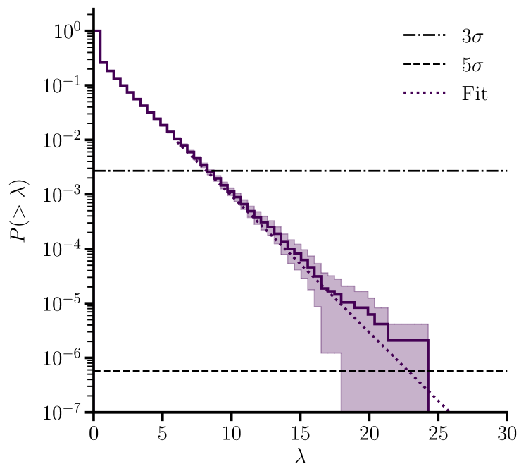
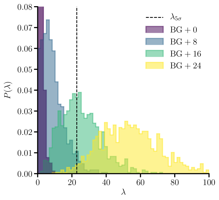
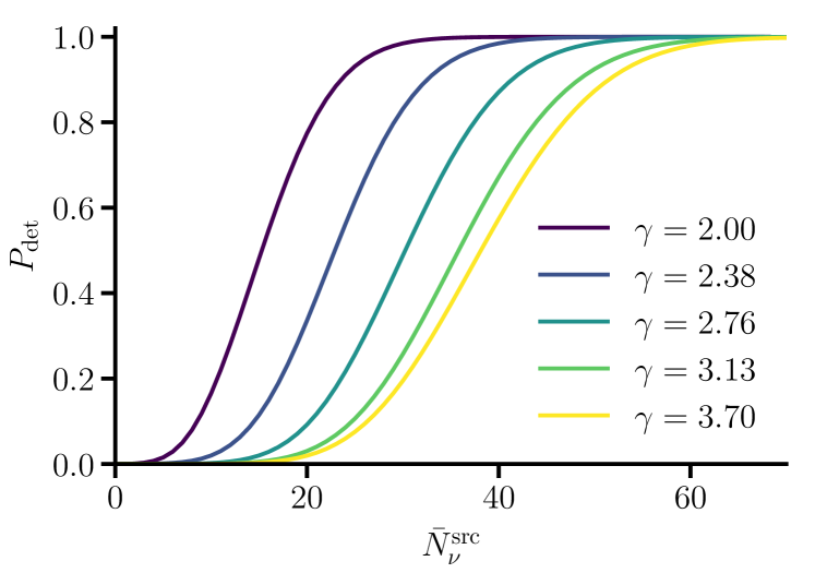
First, we find $\lambda_{5\sigma}$ by evaluating the $\lambda$ distribution for a large number of background simulations. The resulting cumulative probability distribution is shown in Fig. 11. We then inject a fixed number of signal events into the simulation and evaluate the $\lambda$ distribution in this case, as shown in Fig. 12. The detection probability for a given mean number of source events, $\bar{N}_{\nu}^{\mathrm{src}}$, is calculated by summing over the detection probabilities for source events, $N_{\nu}^{\mathrm{src}}$, in the range 0 - 100 and weighting by the Poisson probability, $P(N_{\nu}^{\mathrm{src}}|\bar{N}_{\nu}^{\mathrm{src}})$. The resulting detection probability is shown for a range of spectral indices in Fig. 13.

For a given detector effective area and $\gamma$, $\bar{N}_{\nu}^{\mathrm{src}}$ corresponds to the point source flux normalization, $\phi$, as shown in Equation (11). Using the expression for the point source flux given in Equation (7), we see that

$$P(\mathrm{det}|\bar{N}_{\nu}^{\mathrm{src}},\gamma,\omega_{s})\Leftrightarrow P(\mathrm{det}|\phi,\gamma,\omega_{s}).$$ (25)

In this way, the detection probability can be connected to the source parameters described in Section II, and form part of the generative model.

Figure 11: The $\lambda$ distribution for the simulated background is shown with the $\pm\sqrt{N_{\mathrm{bin}}}$ uncertainty as the shaded area, with $N_{\mathrm{bin}}$ the number of counts in each histogram bin (c.f. Fig. 6 in Braun et al. [38]). For this example we have calculated $\lambda$ in $4.8\times 10^{5}$ trials. The $3\sigma$ and $5\sigma$ levels are also plotted as the dash-dotted and dashed lines, respectively. An exponential function is fit to the tail of the distribution to determine $\lambda_{5\sigma}=22.8$, and this is also shown by the purple dashed line.

Figure 12: The $\lambda$ distribution for simulated background with a varying number of source events (c.f. Fig 6 in Braun et al. [38]). $10^{3}$ trials are shown for each case, and the injected signal has a power-law spectrum with $\gamma=2$. The dashed line shows $\lambda_{5\sigma}$, the threshold for a $5\sigma$ detection, and we see that injecting 16 source events corresponds to $P_{\mathrm{det}}\sim 0.5$.

Figure 13: The detection probability as a function of the expected source counts, $\bar{N}_{\nu}^{\mathrm{src}}$. The case for $\gamma=2$ is shown, based on the results presented in Fig. 12, with steeper $\gamma$ shown for comparison. As expected, a steeper source spectrum requires more source counts for detection as it is more difficult to distinguish the signal events from the background (c.f. Fig. 7 and Fig. 8 in Braun et al. [38]).

Appendix C Impact of including $\mathbf{n_{0}}$ and $\theta$ into the detection probability

Changing the population density and evolution parameters, $n_{0}$ and $\theta$, results in a variation of the diffuse astrophysical flux, which is a background to point source detection. As we require the diffuse astrophysical flux to match observations in our joint model, in practice, the value of the diffuse astrophysical flux is somewhat constrained, and this change will have a limited impact on our results. However, in the low $n_{0}$ regime, we have the extreme case of only a few sources in the population and effectively no diffuse astrophysical background to source detection, leading to more constraining results. Here, we explore this extreme case and demonstrate that it has little impact on our final results.

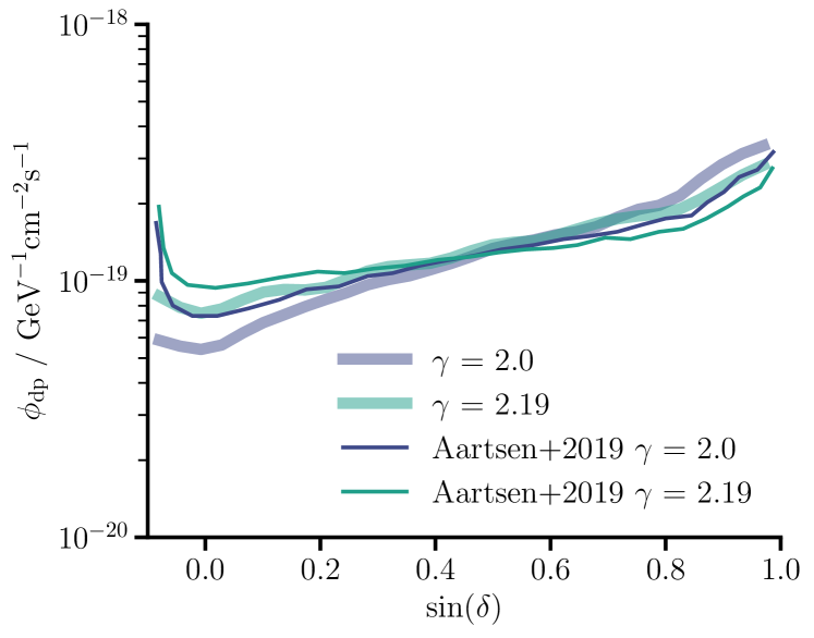
Fig. 14 shows the discovery potential in the case of a diffuse background that is purely due to the atmospheric neutrino flux. The results are similar to what we find in Fig. 2, but we see a slight decrease in $\phi_{\mathrm{dp}}$ at low declinations. This decrease is due to the fact that at lower declinations, even the highest energy neutrinos are not attenuated due to Earth-absorption, and by removing the astrophysical background, we become more sensitive to high energy point source signals.

Figure 14: The discovery potential, as calculated in Fig. 2, but for the case of a purely atmospheric diffuse background flux.

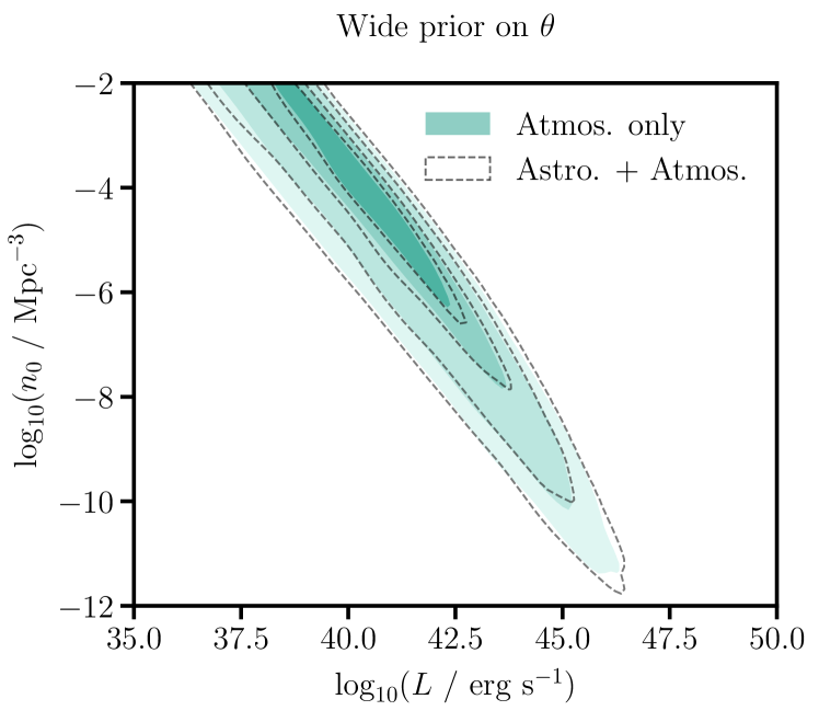
We now calculate the detection probability for this case, as in Section IV.2, and propagate this through into our final results for the population parameters $n_{0}$ and $L$, which are shown in Fig. 15. We see good agreement between the two cases with no apparent differences.

Figure 15: The joint posterior distribution, as in the bottom-left panel of Fig. 6, but for the case of a purely atmospheric diffuse background flux in the detection probability calculation. The standard case of both astrophysical and atmospheric diffuse background components is also shown for comparison.

Appendix D Full posterior derivation

In Section V.3, we present the expression in Equation (22) as the form of the posterior distribution. Here, we derive this expression in full. The posterior distribution is defined over the model parameters, $\theta$, $n_{0}$, $L$, $\bar{N}_{\mathrm{s}}$ and $\bar{N}_{\mathrm{s}}^{\mathrm{tot}}$, and is conditional on the observations, $N_{\mathrm{s}}$, $\hat{\Phi}$, $\hat{\gamma}$, and the model assumptions, $M$. This gives us

$$P(\theta,n_{0},L,\gamma,\bar{N}_{\mathrm{s}},\bar{N}_{\mathrm{s}}^{\mathrm{tot}}\Phi|N_{\mathrm{s}},\hat{\Phi},\hat{\gamma},M)\propto P(\theta,n_{0},L,\gamma,\bar{N}_{\mathrm{s}},\bar{N}_{\mathrm{s}}^{\mathrm{tot}},\Phi|M)P(N_{\mathrm{s}},\hat{\Phi},\hat{\gamma}|\theta,n_{0},L,\gamma,\bar{N}_{\mathrm{s}},\bar{N}_{\mathrm{s}}^{\mathrm{tot}},\Phi,M),$$ (26)

where we have used Bayes’ theorem to expand the posterior. In a complex hierarchical model with many latent parameters, it is not always clear how to factorize terms into the prior and likelihood function, as typically done for simpler examples. However, for the purpose of this derivation, we consider the first term to be the joint prior distribution, and the second term the joint likelihood. We can proceed by expanding the prior term using the chain rule, to separate out the hyperparameters from the latent parameters. This gives

$$P(\theta,n_{0},L,\gamma,\bar{N}_{\mathrm{s}},\bar{N}_{\mathrm{s}}^{\mathrm{tot}},\Phi|M)=P(\theta,n_{0},L,\gamma|M)P(\bar{N}_{\mathrm{s}},\bar{N}_{\mathrm{s}}^{\mathrm{tot}},\Phi|\theta,n_{0},L,\gamma),$$ (27)

where the first term is the joint prior over the hyperparameters. In our model, we treat $\theta$, $n_{0}$, $L$ and $\gamma$ as independent, and this term factorizes into independent probabilities. In expanding the second term , we have also used conditional independence to write this as independent of $M$. The second term can also be factorized further using the conditional independence of $\bar{N}_{\mathrm{s}}$, $\bar{N}_{\mathrm{s}}^{\mathrm{tot}}$ and $\Phi$ such that

$$P(\theta,n_{0},L,\gamma,\bar{N}_{\mathrm{s}},\bar{N}_{\mathrm{s}}^{\mathrm{tot}},\Phi|M)=P(\theta,n_{0},L,\gamma|M)P(\bar{N}_{\mathrm{s}}|\theta,n_{0},L,\gamma)P(\bar{N}_{\mathrm{s}}^{\mathrm{tot}}|n_{0},\theta)P(\Phi|\theta,n_{0},L,\gamma).$$ (28)

We continue by now considering the likelihood factor in our original expression for the posterior distribution. Again, we start by expanding the expression using the chain rule and separating out independent observations from those that are connected, which yields

$$P(N_{\mathrm{s}},\hat{\Phi},\hat{\gamma}|\theta,n_{0},L,\gamma,\bar{N}_{\mathrm{s}},\bar{N}_{\mathrm{s}}^{\mathrm{tot}},\Phi,M)=P(\hat{\gamma}|\theta,n_{0},L,\gamma,\bar{N}_{\mathrm{s}},\bar{N}_{\mathrm{s}}^{\mathrm{tot}},\Phi,M)P(N_{\mathrm{s}},\hat{\Phi}|\theta,n_{0},L,\gamma,\bar{N}_{\mathrm{s}},\bar{N}_{\mathrm{s}}^{\mathrm{tot}},\Phi,M).$$ (29)

We now make use of conditional independence of $\hat{\gamma}$, $N_{\mathrm{s}}$ and $\hat{\Phi}$ to simplify this expression as much as possible

$$P(N_{\mathrm{s}},\hat{\Phi},\hat{\gamma}|\theta,n_{0},L,\gamma,\bar{N}_{\mathrm{s}},\bar{N}_{\mathrm{s}}^{\mathrm{tot}},\Phi,M)=P(\hat{\gamma}|\gamma)P(N_{\mathrm{s}}|\bar{N}_{\mathrm{s}})P(\hat{\Phi}|\bar{N}_{\mathrm{s}}^{\mathrm{tot}},\Phi).$$ (30)

In the regime of large $n_{0}$, $\hat{\Phi}$ is independent of $N_{\mathrm{s}}^{\mathrm{tot}}$. However, in the low $n_{0}$ limit, we enter the regime where could be very few sources in the observable universe, and the detected astrophysical flux is conditionally dependent on the presence or lack of sources. We can treat this by expanding the final term as a mixture model over the case where $N_{\mathrm{s}}^{\mathrm{tot}}=0$ and its complement, as shown in Equation (21). Bringing this all together, we have the complete expression shown in Equation (22).

$$\begin{split}P(\theta,n_{0},\gamma,\bar{N}_{\mathrm{s}},&\bar{N}_{\mathrm{s}}^{\mathrm{tot}},\Phi|N_{\mathrm{s}},\hat{\Phi},\hat{\gamma},M)\\ &\propto P(\theta,n_{0},L,\gamma|M)P(\bar{N}_{\mathrm{s}}|\theta,n_{0},L,\gamma)P(\bar{N}_{\mathrm{s}}^{\mathrm{tot}}|n_{0},\theta)P(\Phi|\theta,n_{0},L,\gamma)P(\hat{\gamma}|\gamma)P(N_{\mathrm{s}}|\bar{N}_{\mathrm{s}})P(\hat{\Phi}|\bar{N}_{\mathrm{s}}^{\mathrm{tot}},\Phi).\end{split}$$ (31)

References

- Mészáros et al. [2019] P. Mészáros, D. B. Fox, C. Hanna, and K. Murase, Multi-messenger astrophysics, Nature Reviews Physics 1, 585 (2019).
- Halzen [2017] F. Halzen, High-energy neutrino astrophysics, Nature Physics 13, 232 (2017).
- Aartsen et al. [2013] M. G. Aartsen et al., Evidence for High-Energy Extraterrestrial Neutrinos at the IceCube Detector, Science 342, 1242856 (2013).
- Aartsen et al. [2015a] M. G. Aartsen, M. Ackermann, J. Adams, J. A. Aguilar, M. Ahlers, et al., A combined maximum-likelihood analysis of the high-energy astrophysical neutrino flux measured with IceCube, The Astrophysical Journal 809, 98 (2015a).
- Aartsen et al. [2014] M. G. Aartsen, M. Ackermann, J. Adams, J. A. Aguilar, M. Ahlers, M. Ahrens, D. Altmann, T. Anderson, C. Argüelles, T. C. Arlen, and et al., Observation of high-energy astrophysical neutrinos in three years of icecube data, Physical Review Letters 113, 101101 (2014).
- Aartsen et al. [2016] M. G. Aartsen et al., Observation and characterization of a cosmic muon neutrino flux from the Northern hemisphere using six years of IceCube data, The Astrophysical Journal 833, 3 (2016).
- Abbasi et al. [2011] R. Abbasi et al., Time-integrated searches for point-like source of neutrinos with the 40-string IceCube detector, The Astrophysical Journal 732, 18 (2011).
- Aartsen et al. [2017a] M. G. Aartsen et al., All-sky Search for Time-integrated Neutrino Emission from Astrophysical Sources with 7 yr of IceCube Data, The Astrophysical Journal 835, 151 (2017a).
- Aartsen et al. [2019a] M. G. Aartsen et al., Search for steady point-like sources in the astrophysical muon neutrino flux with 8 years of IceCube data, Eur. Phys. J. C 79, 234 (2019a).
- Aartsen et al. [2019b] M. G. Aartsen et al., Search for Sources of Astrophysical Neutrinos Using Seven Years of IceCube Cascade Events, The Astrophysical Journal 886, 12 (2019b).
- Aartsen et al. [2020] M. G. Aartsen, M. Ackermann, J. Adams, J. A. Aguilar, M. Ahlers, et al., Time-Integrated Neutrino Source Searches with 10 Years of IceCube Data, Physical Review Letters 124, 051103 (2020).
- Aartsen et al. [2017b] M. G. Aartsen et al., Constraints on Galactic Neutrino Emission with Seven Years of IceCube Data, The Astrophysical Journal 849, 67 (2017b).
- Mészáros [2017] P. Mészáros, Astrophysical Sources of High-Energy Neutrinos in the IceCube Era, Annual Review of Nuclear and Particle Science 67, 45 (2017).
- Lipari [2006] P. Lipari, Perspectives of high-energy neutrino astronomy, Nuclear Instruments and Methods in Physics Research Section A: Accelerators, Spectrometers, Detectors and Associated Equipment 567, 405 (2006).
- Lipari [2008] P. Lipari, Proton and neutrino extragalactic astronomy, Physical Review D 78, 083011 (2008).
- Silvestri and Barwick [2010] A. Silvestri and S. W. Barwick, Constraints on extragalactic point source flux from diffuse neutrino limits, Physical Review D 81, 023001 (2010).
- Murase et al. [2012] K. Murase, J. F. Beacom, and H. Takami, Gamma-ray and neutrino backgrounds as probes of the high-energy universe: hints of cascades, general constraints, and implications for TeV searches, J. Cosmol. Astropart. P. 08, 030 (2012).
- Ahlers and Halzen [2014] M. Ahlers and F. Halzen, Pinpointing extragalactic neutrino sources in light of recent IceCube observations, Physical Review D 90, 043005 (2014).
- Kowalski [2015] M. Kowalski, Status of High-Energy Neutrino Astronomy, Journal of Physics: Conference Series 632, 012039 (2015).
- Murase and Waxman [2016] K. Murase and E. Waxman, Constraining High-Energy Cosmic Neutrino Sources: Implications and Prospects, Physical Review D D94, 103006 (2016).
- Palladino et al. [2019] A. Palladino, A. van Vliet, W. Winter, and A. Franckowiak, Can astrophysical neutrinos trace the origin of the detected ultra-high energy cosmic rays?, arXiv.org (2019), 1911.05756v1 .
- Bartos et al. [2017] I. Bartos, M. Ahrens, C. Finley, and S. Márka, Prospects of establishing the origin of cosmic neutrinos using source catalogs, Physical Review D 96, 023003 (2017).
- Madau and Dickinson [2014] P. Madau and M. Dickinson, Cosmic star formation history, Annu. Rev. Astron. Astrophys. 52, 415–486 (2014).
- Aird et al. [2010] J. Aird, K. Nandra, E. S. Laird, A. Georgakakis, M. L. N. Ashby, P. Barmby, A. L. Coil, J. S. Huang, A. M. Koekemoer, C. C. Steidel, and C. N. A. Willmer, The evolution of the hard X-ray luminosity function of AGN, Monthly Notices of the Royal Astronomical Society 401, 2531 (2010).
- Taylor et al. [2015] A. M. Taylor, M. Ahlers, and D. Hooper, Indications of negative evolution for the sources of the highest energy cosmic rays, Physical Review D 92, 063011 (2015).
- Aab and others [2018] A. Aab and others, Combined fit of spectrum and composition data as measured by the Pierre Auger Observatory, J. Cosmol. Astropart. P. 1704, 038 (2018).
- Batista et al. [2019] R. A. Batista, R. M. de Almeida, B. Lago, and K. Kotera, Cosmogenic photon and neutrino fluxes in the Auger era, J. Cosmol. Astropart. P. 2019, 002 (2019).
- Ajello et al. [2014] M. Ajello, R. W. Romani, D. Gasparrini, M. S. Shaw, J. Bolmer, G. Cotter, J. Finke, J. Greiner, S. E. Healey, O. King, W. Max-Moerbeck, P. F. Michelson, W. J. Potter, A. Rau, A. C. S. Readhead, J. L. Richards, and P. Schady, The cosmic evolution of Fermi BL Lacertae objects, The Astrophysical Journal 780, 73 (2014).
- Cole et al. [2001] S. Cole, P. Norberg, C. M. Baugh, et al., The 2dF galaxy redshift survey: near-infrared galaxy luminosity functions, Monthly Notices of the Royal Astronomical Society 326, 255 (2001).
- Ueda et al. [2003] Y. Ueda, M. Akiyama, K. Ohta, and T. Miyaji, Cosmological evolution of the hard X-ray active galactic nucleus luminosity function and the origin of the hard X-ray background, The Astrophysical Journal 598, 886 (2003).
- Peacock [2010] J. A. Peacock, Cosmological Physics (Cambridge University Press, Cambridge, United Kingdom, 2010) pp. 89–91.
- Achterberg et al. [2006] A. Achterberg et al., First year performance of the IceCube neutrino telescope, Astroparticle Physics 26, 155 (2006).
- Aartsen et al. [2017c] M. G. Aartsen et al., The IceCube Neutrino Observatory: instrumentation and online systems, Journal of Instrumentation 12, 03012 (2017c).
- Gaisser et al. [2016] T. K. Gaisser, R. Engel, and E. Resconi, Cosmic rays and particle physics, second edition (Cambridge University Press, Cambridge, United Kingdom, 2016) p. 362.
- Learned and Pakvasa [1995] J. G. Learned and S. Pakvasa, Detecting oscillations at PeV energies, Astroparticle Physics 3, 267 (1995).
- Athar et al. [2011] H. Athar, C. S. Kim, and J. Lee, Intrinsic and oscillated astrophysical neutrino flavor ratios revisited, Modern Physics Letters A 21, 1049 (2011).
- Aartsen et al. [2018a] M. G. Aartsen, M. Ackermann, J. Adams, J. A. Aguilar, M. Ahlers, M. Ahrens, D. Altmann, T. Anderson, C. Argüelles, T. C. Arlen, J. Auffenberg, X. Bai, S. W. Barwick, V. Baum, J. J. Beatty, J. B. Tjus, K. H. Becker, et al., All-sky point-source icecube data: years 2010-2012, https://icecube.wisc.edu/science/data/PS-3years (2018a), dataset.
- Braun et al. [2008] J. Braun, J. Dumm, F. De Palma, C. Finley, A. Karle, and T. Montaruli, Methods for point source analysis in high energy neutrino telescopes, Astroparticle Physics 29, 299 (2008).
- Aartsen et al. [2015b] M. G. Aartsen, M. Ackermann, J. Adams, J. A. Aguilar, M. Ahlers, M. Ahrens, D. Altmann, T. Anderson, C. Argüelles, T. C. Arlen, J. Auffenberg, X. Bai, S. W. Barwick, V. Baum, J. J. Beatty, J. B. Tjus, K. H. Becker, et al., Development of a general analysis and unfolding scheme and its application to measure the energy spectrum of atmospheric neutrinos with IceCube, Eur. Phys. J. C 75, 116 (2015b).
- Aartsen et al. [2015c] M. G. Aartsen et al., Evidence for Astrophysical Muon Neutrinos from the Northern Sky with IceCube, Physical Review Letters 115, 081102 (2015c).
- Haack and Wiebusch [2017] C. Haack and C. Wiebusch, A measurement of the diffuse astrophysical muon neutrino flux using eight years of icecube data, in Proceedings of the 35th International Cosmic Ray Conference (ICRC2017) (2017) p. PoS(ICRC2017)1005.
- Kruschke and Liddell [2017] J. K. Kruschke and T. M. Liddell, The Bayesian New Statistics: Hypothesis testing, estimation, meta-analysis, and power analysis from a Bayesian perspective, Psychonomic Bulletin & Review 25, 178 (2017).
- Gelman et al. [2014] A. Gelman, J. B. Carlin, H. S. Stern, D. B. Dunson, A. Vehtari, and D. B. Rubin, Bayesian Data Analysis (CRC Press, Boca Raton, Florida, 2014).
- Wilks [1938] S. S. Wilks, The Large-Sample Distribution of the Likelihood Ratio for Testing Composite Hypotheses, The Annals of Mathematical Statistics 9, 60 (1938).
- Simpson et al. [2017] D. Simpson, H. Rue, A. Riebler, T. G. Martins, and S. H. Sørbye, Penalising Model Component Complexity: A Principled, Practical Approach to Constructing Priors, Statistical Science 32, 1 (2017).
- Carpenter et al. [2017] B. Carpenter, A. Gelman, M. D. Hoffman, D. Lee, B. Goodrich, M. Betancourt, M. Brubaker, J. Guo, P. Li, and A. Riddell, Stan: A Probabilistic Programming Language, Journal of Statistical Software 76, 1 (2017).
- Betancourt et al. [2017] M. Betancourt, S. Byrne, S. Livingstone, and M. Girolami, The geometric foundations of Hamiltonian Monte Carlo, Bernoulli 23, 2257 (2017).
- Aartsen and others [2014] M. G. Aartsen and others, IceCube-Gen2: A Vision for the Future of Neutrino Astronomy in Antarctica, arXiv.org (2014), 1412.5106 .
- van Santen [2017] J. van Santen, IceCube-Gen2: the next-generation neutrino observatory for the South Pole, in Proceedings of the 35th International Cosmic Ray Conference (2017) p. 991.
- Dekker and Ando [2018] A. Dekker and S. Ando, Angular power spectrum analysis on current and future high-energy neutrino data, Journal of Cosmology and Astroparticle Physics 2019 (02), 002–002.
- Adrián-Martínez et al. [2016] S. Adrián-Martínez, M. Ageron, F. Aharonian, S. Aiello, et al., Letter of intent for KM3NeT 2.0, Journal of Physics G: Nuclear and Particle Physics 43, 084001 (2016).
- Aiello et al. [2019] S. Aiello, S. E. Akrame, F. Ameli, et al., Sensitivity of the KM3NeT/ARCA neutrino telescope to point-like neutrino sources, Astroparticle Physics 111, 100 (2019).
- The IceCube Collaboration et al. [2018] The IceCube Collaboration, Fermi-LAT, MAGIC, AGILE, ASAS-SN, HAWC, H.E.S.S., INTEGRAL, Kanata, Kiso, Kapteyn, Liverpool Telescope, Subaru, Swift/NuSTAR, VERITAS, and VLA/17B-403 teams, Multimessenger observations of a flaring blazar coincident with high-energy neutrino IceCube-170922A, Science 361, eaat1378 (2018).
- Aartsen et al. [2018b] M. G. Aartsen et al., Neutrino emission from the direction of the blazar TXS 0506+056 prior to the IceCube-170922A alert, Science 361, 147 (2018b).
- Padovani et al. [2019] P. Padovani, F. Oikonomou, M. Petropoulou, P. Giommi, and E. Resconi, TXS 0506+056, the first cosmic neutrino source, is not a BL Lac, Monthly notices of the Royal Astronomical Society 484, L104 (2019), 1901.06998v1 .
- Waxman and Bahcall [1998] E. Waxman and J. Bahcall, High energy neutrinos from astrophysical sources: An upper bound, Physical Review D 59, 023002 (1998).
- Ackermann et al. [2015] M. Ackermann, M. Ajello, A. Albert, et al., The spectrum of diffuse gamma-ray emission between 100 MeV and 820 GeV, The Astrophysical Journal 799, 86 (2015).
- Murase et al. [2013] K. Murase, M. Ahlers, and B. C. Lacki, Testing the hadronuclear origin of PeV neutrinos observed with IceCube, Physical Review D 88, 121301(R) (2013).
- Capanema et al. [2020] A. Capanema, A. Esmaili, and K. Murase, New Constraints on the Origin of Medium-Energy Neutrinos Observed by IceCube, arXiv.org (2020), 2002.07192v1 .
- Oliphant [2006] T. Oliphant, A guide to NumPy (Trelgol Publishing, 2006).
- Jones et al. [2001] E. Jones, T. Oliphant, P. Peterson, et al., SciPy: Open source scientific tools for Python (2001), accessed on the 3rd April 2020.
- Price-Whelan et al. [2018] A. M. Price-Whelan, B. M. Sip’ocz, H. M. Günther, et al., The Astropy Project: Building an Open-science Project and Status of the v2.0 Core Package, aj 156, 123 (2018).
- Hunter [2007] J. D. Hunter, Matplotlib: A 2D Graphics Environment, Comput. Sci. Eng. 9, 90 (2007).
- Waskom et al. [2017] M. Waskom, O. Botvinnik, D. O’Kane, P. Hobson, S. Lukauskas, D. C. Gemperline, T. Augspurger, Y. Halchenko, J. B. Cole, J. Warmenhoven, J. de Ruiter, C. Pye, S. Hoyer, J. Vanderplas, S. Villalba, G. Kunter, E. Quintero, P. Bachant, M. Martin, K. Meyer, A. Miles, Y. Ram, T. Yarkoni, M. L. Williams, C. Evans, C. Fitzgerald, Brian, C. Fonnesbeck, A. Lee, and A. Qalieh, mwaskom/seaborn: v0.8.1 (september 2017) (2017).
- Collette [2013] A. Collette, Python and HDF5 (O’Reilly, 2013).