Fitting Laplacian Regularized
Stratified Gaussian Models

Abstract

We consider the problem of jointly estimating multiple related zero-mean Gaussian distributions from data. We propose to jointly estimate these covariance matrices using Laplacian regularized stratified model fitting, which includes loss and regularization terms for each covariance matrix, and also a term that encourages the different covariances matrices to be close. This method ‘borrows strength’ from the neighboring covariances, to improve its estimate. With well chosen hyper-parameters, such models can perform very well, especially in the low data regime. We propose a distributed method that scales to large problems, and illustrate the efficacy of the method with examples in finance, radar signal processing, and weather forecasting.

1 Introduction

We observe data records of the form $(z,y)$, where $y\in{\mbox{\bf R}}^{n}$ and $z\in\{1,\ldots,K\}$. We model $y$ as samples from a zero-mean Gaussian distribution, conditioned on $z$, i.e.,

$$y\mid z\sim\mathcal{N}(0,\Sigma_{z}),$$

with $\Sigma_{z}\in{\mbox{\bf S}}_{++}^{n}$ (the set of symmetric positive definite $n\times n$ matrices), $z=1,\ldots,K$. Our goal is to estimate the model parameters $\Sigma=(\Sigma_{1},\ldots,\Sigma_{K})\in({\mbox{\bf S}}_{++}^{n})^{K}$ from the data. We refer to this as a stratified Gaussian model, since we have a different Gaussian model for $y$ for each value of the stratification feature $z$. Estimating a set of covariance matrices is referred to as joint covariance estimation.

The negative log-likelihood of $\Sigma$, on an observed data set $(z_{i},y_{i})$, $i=1,\ldots,m$, is given by

$$\sum_{i=1}^{m}\left((1/2)y_{i}^{T}\Sigma_{z_{i}}^{-1}y_{i}-(1/2)\log\det(\Sigma_{z_{i}}^{-1})-(n/2)\log(2\pi)\right)$$

$$= \sum_{k=1}^{K}\left((n_{k}/2)\mathop{\bf Tr}(S_{k}\Sigma_{k}^{-1})-(n_{k}/2)\log\det(\Sigma_{k}^{-1})-(n_{k}n/2)\log(2\pi)\right),$$

where $n_{k}$ is the number of data samples with $z=k$ and $S_{k}=\frac{1}{n_{k}}\sum_{i:z_{i}=k}y_{i}y_{i}^{T}$ is the empirical covariance matrix of $y$ for which $z=k$, with $S_{k}=0$ when $n_{k}=0$.

This function is general not convex in $\Sigma$, but it is convex in the natural parameter

$$\theta=(\theta_{1},\ldots,\theta_{K})\in({\mbox{\bf S}}_{++}^{n})^{K},$$

where $\theta_{k}=\Sigma_{k}^{-1}$, $k=1\ldots,K$. We will focus on estimating $\theta$ rather than $\Sigma$. In terms of $\theta$, and dropping a constant and a factor of two, the negative log-likelihood is

$$\ell(\theta)=\sum_{k=1}^{K}\ell_{k}(\theta_{k}),$$

where

$$\ell_{k}(\theta_{k})=n_{k}\left(\mathop{\bf Tr}(S_{k}\theta_{k})-\log\det(\theta_{k})\right).$$

We refer to $\ell(\theta)$ as the loss, and $\ell_{k}(\theta_{k})$ as the local loss, associated with $z=k$. For the special case where $n_{k}=0$, we define $\ell_{k}(\theta_{k})$ to be zero if $\theta_{k}\succ 0$, and $\infty$ otherwise. We refer to $\ell(\theta)/m$ as the average loss.

To estimate $\theta$, we add two types of regularization to the loss, and minimize the sum. We choose $\theta$ as a solution of

$$\begin{array}[]{ll}\mbox{minimize}&\sum_{k=1}^{K}\left({\ell_{k}}(\theta_{k})+r(\theta_{k})\right)+\mathcal{L}(\theta),\end{array}$$ (1)

where $\theta$ is the optimization variable, $r:{\mbox{\bf S}}^{n}\to{\mbox{\bf R}}$ is a local regularization function, and $\mathcal{L}:({\mbox{\bf S}}^{n})^{K}\to{\mbox{\bf R}}$ is Laplacian regularization, defined below. We refer to our estimated $\theta$ as a Laplacian regularized stratified Gaussian model.

Local regularization.

Common types of local regularization include trace regularization, $r(\theta_{k})=\gamma\mathop{\bf Tr}\theta_{k}$, and Frobenius regularization, $r(\theta_{k})=\gamma\|\theta_{k}\|_{F}^{2}$, where $\gamma>0$ is a hyper-parameter. Two more recently introduced local regularization terms are $\gamma\|\theta_{k}\|_{1}$ and $\gamma\|\theta_{k}\|_{\mathrm{od},1}=\gamma\sum_{i\neq j}|(\theta_{k})_{ij}|$, which encourage sparsity of $\theta$ and of the off-diagonal elements of $\theta$, respectively [FHT08]. (A zero entry in $\theta_{k}$ means that the associated components of $y$ are conditionally indedendent, given the others, when $z=k$ [DWW14].)

Laplacian regularization.

Let $W\in{\mbox{\bf S}}^{K}$ be a symmetric matrix with zero diagonal entries and nonnegative off-diagonal entries. The associated Laplacian regularization is the function $\mathcal{L}:({\mbox{\bf S}}^{n})^{K}\to{\mbox{\bf R}}$ given by

$$\mathcal{L}(\theta)=\frac{1}{2}\sum_{i,j=1}^{K}W_{ij}\|\theta_{i}-\theta_{j}\|_{F}^{2}.$$

Evidently $\mathcal{L}$ is separable across the entries of its arguments; it can be expressed as

$$\mathcal{L}(\theta)=\frac{1}{2}\sum_{u,v=1}^{n}\left(\sum_{i,j=1}^{K}W_{ij}((\theta_{i})_{uv}-(\theta_{j})_{uv})^{2}\right).$$

Laplacian regularization encourages the estimated values of $\theta_{i}$ and $\theta_{j}$ to be close when $W_{ij}>0$. Roughly speaking, we can interpret $W_{ij}$ as prior knowledge about how close the data generation processes for $y$ are, for $z=i$ and $z=j$.

We can associate the Laplacian regularization with a graph with $K$ vertices, which has an edge $(i,j)$ for each positive $W_{ij}$, with weight $W_{ij}$. We refer to this graph as the regularization graph. We assume that the regularization graph is connected. We can express Laplacian regularization in terms of a (weighted) Laplacian matrix $L$, given by

$$L_{ij}=\left\{\begin{array}[]{ll}-W_{ij}&i\neq j\\ \sum_{k=1}^{K}W_{ik}&i=j\end{array}\right.$$

for $i,j=1,\ldots,K$. The Laplacian regularization can be expressed in terms of $L$ as

$${\mathcal{L}}(\theta)=(1/2)\mathop{\bf Tr}(\theta^{T}(I\otimes L)\theta),$$

where $\otimes$ denotes the Kronecker product.

Assumptions.

We note that (1) need not have a unique solution, in pathological cases. As a simple example, consider the case with $r=0$ and $W=0$, i.e., no local regularization and no Laplacian regularization, which corresponds to independently creating a model for each value of $z$. If all $S_{k}$ are positive definite, the solution is unique, with $\theta_{k}=S_{k}^{-1}$. If any $S_{k}$ is not positive definite, the problem does not have a unique solution. The presence of either local or Laplacian regularization (with the associated graph being connected) can ensure that the problem has a unique solution. For example, with trace regularization (and $\gamma>0$), it is readily shown that the problem (1) has a unique solution. Another elementary condition that guarantees a unique solution is that the associated graph is connected, and $S_{k}$ do not have a common nullspace.

We will henceforth assume that the problem (1) has a unique solution. This implies that the objective in (1) is closed, proper, and convex. The problem (1) is a convex optimization problem which can be solved globally in an efficient manner [VB96, BV04].

Contributions.

Joint covariance estimation and Laplacian regularized stratified model fitting are not new ideas; in this paper we simply bring them together. Laplacian regularization has been shown to work well in conjunction with stratified models, allowing one with very little data to create sensible models for each value of some stratification parameter [TBB19, TB20]. To our knowledge, this is the first paper that has explicitly framed joint covariance estimation as a stratified model fitting problem. We develop and implement a large-scale distributed method for Laplacian regularized joint covariance estimation via the alternating direction method of multipliers (ADMM), which scales to large-scale data sets [BPC⁺11, WBAW12].

Outline.

In §1, we introduce Laplacian regularized stratified Gaussian models and review work related to fitting Laplacian regularized stratified Gaussian models. In §2, we develop and analyze a distributed solution method to fit Laplacian regularized stratified Gaussian models, based on ADMM. Lastly, in §3, we illustrate the efficacy of this model fitting technique and of this method with three examples, in finance, radar signal processing, and weather forecasting.

1.1 Related work

Stratified model fitting.

Stratified model fitting, i.e., separately fitting a different model for each value of some parameter, is an idea widely used across disciplines. For example, in medicine, patients are often divided into subgroups based on age and sex, and one fits a separate model for the data from each subgroup [KVM⁺99, TBB19]. Stratification can be useful for dealing with categorical feature values, interpreting the nature of the data, and can play a large role in experiment design. As mentioned previously, the joint covariance estimation problem can naturally be framed as a stratified model fitting problem.

Covariance matrix estimation.

Covariance estimation applications span disciplines such as radar signal processing [SCC⁺19], statistical learning [BEGd08], finance [AC00, SB09], and medicine [LH87]. Many techniques exist for the estimation of a single covariance matrix when the covariance matrix’s structure is known a priori [FLL16]. When the covariance matrix is sparse, thresholding the elements of the sample covariance matrix has been shown to be an effective method of covariance matrix estimation [BL08]. [SG00] propose a maximum likelihood solution for a covariance matrix that is the sum of a Hermitian positive semidefinite matrix and a multiple of the identity. Maximimum likelihood-style approaches also exist for when the covariance matrix is assumed to be Hermitian, Toeplitz, or both [BLW82, MS87, LSL99]. [CB09] propose using various shrinkage estimators when the data is high dimensional. (Shrinkage parameters are typically chosen by an out-of-sample validation technique [HL96].)

Joint covariance estimation.

Jointly estimating statistical model parameters has been the subject of significant research spanning different disciplines. The joint graphical lasso [DWW14] is a stratified model that encourages closeness of parameters by their difference as measured by fused lasso and group lasso penalties. (Laplacian regularization penalizes their difference by the $\ell_{2}$-norm squared.) The joint graphical lasso penalties in effect result in groups of models with the same parameters, and those parameters being sparse. (In contrast, Laplacian regularization leads to parameter values that vary smoothly with nearby models. It has been observed that in most practical settings, Laplacian regularization is sufficient for accurate estimation [TBB19].) Similar to the graphical lasso, methods such as the time-varying graphical lasso [HPBL17] and the network lasso [HLB15] have been recently developed to infer model parameters in graphical networks assuming some graphical relationship (in the former, the relationship is in time; in the latter, the relationship is arbitrary).

Another closely related work to this paper is [THB19], which introduces the use of Laplacian regularization in joint estimation of covariance matrices in a zero-mean multivariate Gaussian model. In this paper, Laplacian regularization is used assuming a grid structure, and the problem is solved using the majorization-minimization algorithmic framework [SBP17]. In contrast, this paper assumes a much more complex and sophisticated structure of the system, and uses ADMM to solve the problem much more efficiently.

Connection to probabilistic graphical models.

There is a significant connection of this work to probabilistic graphical models [KF09]. In this connection, a stratified model for joint model parameter estimation can be seen as an undirected graphical model, where the vertices follow different distributions, and the edges encourage corresponding vertices’ distributions to be alike. In fact, very similar problems in atmospheric science, medicine, and statistics have been studied under this context [GLMZ11, DWW14, ZSP14, MM16].

2 Distributed solution method

There are many methods that can be used to solve minimize (1); for example, ADMM [BPC⁺11] has been successfully used in the past as a large-scale, distributed method for stratified model fitting with Laplacian regularization [TBB19], which we will adapt for use in this paper. This method expresses minimizing (1) in the equivalent form

$$\begin{array}[]{ll}{{\mbox{minimize}}}&\overset{K}{\underset{k=1}{\sum}}(({\ell_{k}}(\theta_{k})+r(\widetilde{\theta}_{k}))+\mathcal{L}(\widehat{\theta})\\ {\mbox{subject to}}&\theta-\widehat{\theta}=0,\quad\widetilde{\theta}-\widehat{\theta}=0,\end{array}$$ (2)

now with variables $\theta\in({\mbox{\bf S}}_{++}^{n})^{K}$, $\widetilde{\theta}\in({\mbox{\bf S}}_{++}^{n})^{K}$, and $\widehat{\theta}\in({\mbox{\bf S}}_{++}^{n})^{K}$. Problem (2) is in ADMM standard form, splitting on $(\theta,\widetilde{\theta})$ and $\widehat{\theta}$. The ADMM algorithm for this problem, outlined in full in Algorithm 2, can be summarized by four steps: computing the (scaled) proximal operators of $\ell_{1},\ldots,\ell_{K}$, $r$, and $\mathcal{L}$, followed by updates on dual variables associated with the two equality constraints, $U\in({\mbox{\bf R}}^{n\times n})^{K}$ and ${\widetilde{U}}\in({\mbox{\bf R}}^{n\times n})^{K}$. Recall that the proximal operator of $f:{\mbox{\bf R}}^{n\times n}\to{\mbox{\bf R}}$ with penalty parameter $\omega$ is

$$\mathbf{prox}_{\omega f}(V)=\underset{\theta}{\mathop{\rm argmin}}\left(\omega f(\theta)+(1/2)\|\theta-V\|_{F}^{2}\right).$$

• Algorithm 2.1  Distributed method for Laplacian regularized joint covariance estimation.

  given Loss functions $\ell_{1},\ldots,\ell_{K}$, local regularization function $r$, graph Laplacian matrix $L$,
  and penalty parameter $\omega>0$.
  Initialize. $\theta^{0}={\widetilde{\theta}}^{0}={\widehat{\theta}}^{0}=U^{0}={\widetilde{U}}^{0}=0$.
  repeat
  	1. Evaluate the proximal operator of ${\ell_{k}}$. $\theta^{t+1}_{k}=\mathbf{prox}_{\omega\ell_{k}}({\widehat{\theta}}_{k}^{t}-U_{k}^{t}),\quad k=1,\ldots,K$
  	2. Evaluate the proximal operator of $r$. ${\widetilde{\theta}}^{t+1}_{k}=\mathbf{prox}_{\omega r}({\widehat{\theta}}_{k}^{t}-{\widetilde{U}}_{k}^{t}),\quad k=1,\ldots,K$
  	3. Evaluate the proximal operator of $\mathcal{L}$. ${\widehat{\theta}}^{t+1}=\mathbf{prox}_{\omega{\mathcal{L}}/2}((1/2)(\theta^{t+1}+U^{t}+{\widetilde{\theta}}^{t+1}+{\widetilde{U}}^{t}))$
  	4. Update the dual variables. ${{U}}^{t+1}={{U}}^{t}+{\theta}^{t+1}-{\widehat{\theta}}^{t+1};\quad{\widetilde{U}}^{t+1}={\widetilde{U}}^{t}+\widetilde{\theta}^{t+1}-{\widehat{\theta}}^{t+1}$
  until convergence

To see how we could use this for fitting Laplacian regularized stratified models for the joint covariance estimation problem, we outline efficient methods for evaluating the proximal operators of $\ell_{k}$, of a variety of relevant local regularizers $r$, and of the Laplacian regularization.

2.1 Evaluating the proximal operator of $\ell_{k}$

Evaluating the proximal operator of $\ell_{k}$ (for $n_{k}>0$) can be done efficiently and in closed-form [WT09, BPC⁺11, DWW14, TBB19]. We have that the proximal operator is

$$\mathbf{prox}_{\omega\ell_{k}}(V)=QXQ^{T},$$

where $X\in{\mbox{\bf R}}^{K\times K}$ is a diagonal matrix with entries

$$X_{ii}=\frac{\omega n_{k}d_{i}+\sqrt{(\omega n_{k}d_{i})^{2}+4\omega n_{k}}}{2},\quad i=1,\ldots,K,$$

and $d$ and $Q$ are computed as the eigen-decomposition of $(1/\omega n_{k})V-S_{k}$, i.e.,

$$\frac{1}{\omega n_{k}}V-S_{k}=Q\mathop{\bf diag}(d)Q^{T}.$$

The dominant cost in computing the proximal operator of $\ell_{k}$ is in computing the eigen-decomposition, which can be computed with order $n^{3}$ flops.

2.2 Evaluating the proximal operator of $r$

The proximal operator of $r$ often has a closed-form expression that can be computed in parallel. For example, if $r=\gamma\mathop{\bf Tr}(\theta)$, then $\mathbf{prox}_{\omega r}(V)=V-\omega\gamma I$. If $r(\theta)=(\gamma/2)\|\theta\|_{F}^{2}$ then $\mathbf{prox}_{\omega r}(V)=(1/(1+\omega\gamma))V$, and if $r=\gamma\|\theta\|_{1}$, then $\mathbf{prox}_{\omega r}(V)=\max(V-\omega\gamma,0)-\max(-V-\omega\gamma,0)$, where $\max$ is taken elementwise [PB14]. If $r(\theta)=\gamma_{1}\mathop{\bf Tr}(\theta)+\gamma_{2}\|\theta\|_{\mathrm{od},1}$ where $\|\theta\|_{\mathrm{od},1}=\sum_{i\neq j}|\theta_{ij}|$ is the $\ell_{1}$-norm of the off diagonal elements of $\theta$, then

$$\mathbf{prox}_{\omega r}(V)_{ij}=\begin{cases}V_{ij}-\omega\gamma_{1},&i=j\\ \max(V_{ij}-\omega\gamma_{2},0)-\max(-V_{ij}-\omega\gamma_{2},0)&i\neq j\end{cases}.$$

2.3 Evaluating the proximal operator of $\mathcal{L}$

Evaluating the proximal operator of $\mathcal{L}$ is equivalent to solving the $n(n+1)/2$ regularized Laplacian systems

$$\bigg{(}L+(2/\omega)I\bigg{)}\begin{bmatrix}(\widehat{\theta}^{t+1}_{1})_{ij}\\ (\widehat{\theta}^{t+1}_{2})_{ij}\\ \vdots\\ (\widehat{\theta}^{t+1}_{K})_{ij}\end{bmatrix}=(1/\omega)\begin{bmatrix}(\theta^{t+1}_{1}+U^{t}_{1}+{\widetilde{\theta}}^{t+1}_{1}+{\widetilde{U}}^{t}_{1})_{ij}\\ (\theta^{t+1}_{2}+U^{t}_{2}+{\widetilde{\theta}}^{t+1}_{2}+{\widetilde{U}}^{t}_{2})_{ij}\\ \vdots\\ (\theta^{t+1}_{K}+U^{t}_{K}+{\widetilde{\theta}}^{t+1}_{K}+{\widetilde{U}}^{t}_{K})_{ij}\end{bmatrix}$$ (3)

for $i=1,\ldots,n$ and $j=1,\ldots,i$, and setting $({\widehat{\theta}}_{k}^{t+1})_{ji}=({\widehat{\theta}}_{k}^{t+1})_{ij}$. Solving these systems is quite efficient; many methods for solving Laplacian systems (and more generally, symmetric diagonally-dominant systems) can solve these systems in nearly-linear time [Vis13, KOSZ13]. We find that the conjugate gradient (CG) method with a diagonal pre-conditioner [HS52, TJ16] can efficiently and reliably solve these systems. (We can also warm-start CG with $\widehat{\theta}^{t}$.)

Stopping criterion.

Under our assumptions on the objective, the iterates of ADMM converge to a global solution, and the primal and dual residuals

$$r^{t+1}=(\theta^{t+1}-\widehat{\theta}^{t+1},\widetilde{\theta}^{t+1}-\widehat{\theta}^{t+1}),\quad s^{t+1}=-(1/\lambda)(\widehat{\theta}^{t+1}-\widehat{\theta}^{t},\widehat{\theta}^{t+1}-\widehat{\theta}^{t}),$$

converge to zero [BPC⁺11]. This suggests the stopping criterion

$$\|r^{t+1}\|_{F}\leq\epsilon_{\mathrm{pri}},\quad\|s^{t+1}\|_{F}\leq\epsilon_{\mathrm{dual}},$$

for some primal tolerance $\epsilon_{\mathrm{pri}}$ and dual tolerance $\epsilon_{\mathrm{dual}}$. Typically, these tolerances are selected as a combination of absolute and relative tolerances; we use

$$\epsilon_{\mathrm{pri}}=\sqrt{2Kn^{2}}\epsilon_{\mathrm{abs}}+\epsilon_{\mathrm{rel}}\max\{\|r^{t+1}\|_{F},\|s^{t+1}\|_{F}\},\quad\epsilon_{\mathrm{dual}}=\sqrt{2Kn^{2}}\epsilon_{\mathrm{abs}}+(\epsilon_{\mathrm{rel}}/\omega)\|(u^{t},{\widetilde{u}^{t}})\|_{F},$$

for some absolute tolerance $\epsilon_{\mathrm{abs}}>0$ and relative tolerance $\epsilon_{\mathrm{rel}}>0$.

Penalty parameter selection.

In practice (i.e., in §3), we find that the number of iterations to convergence does not change significantly with the choice of the penalty parameter $\omega$. We found that fixing $\omega=0.1$ worked well across all of our experiments.

3 Examples

In this section we illustrate Laplacian regularized stratified model fitting for joint covariance estimation. In each of the examples, we fit two models: a common model (a Gaussian model without stratification), and a Laplacian regularized stratified Gaussian model. For each model, we selected hyper-parameters that performed best under a validation technique. We provide an open-source implementation of Algorithm 2, along with the code used to create the examples, at https://github.com/cvxgrp/strat_models. We train all of our models with an absolute tolerance $\epsilon_{\mathrm{abs}}=10^{-3}$ and a relative tolerance $\epsilon_{\mathrm{rel}}=10^{-3}$. All computation was carried out on a 2014 MacBook Pro with four Intel Core i7 cores clocked at 3 GHz.

3.1 Sector covariance estimation

Estimating the covariance matrix of a portfolio of time series is a central task in quantitative finance, as it is a parameter to be estimated in the classical Markowitz portfolio optimization problem [Mar52, SB09, BBD⁺17]. In addition, models for studying the dynamics of the variance of a time series (or multiple time series) data are common, such as with the GARCH family of models in statistics [Eng82]. In this example, we consider the problem of modeling the covariance of daily sector returns, given market conditions observed the day prior.

Data records and dataset.

We use daily returns from $n=9$ exchange-traded funds (ETFs) that cover the sectors of the stock market, measured daily, at close, from January 1, 2000 to January 1, 2018 (for a total of 4774 data points). The ETFs used are XLB (materials), XLV (health care), XLP (consumer staples), XLY (consumer discretionary), XLE (energy), XLF (financials), XLI (industrials), XLK (technology), and XLU (utilities). Each data record includes $y\in{\mbox{\bf R}}^{9}$, the daily return of the sector ETFs. The sector ETFs have individually been winsorized (clipped) at their 5th and 95th percentiles.

Each data record also includes the market condition $z$, which is derived from market indicators known on the day, the five-day trailing averages of the market volume (as measured by the ETF SPY) and volatility (as measured by the ticker VIX). Each of these market indicators is binned into 2% quantiles (i.e., $0\%-2\%,2\%-4\%,\ldots,98\%-100\%$), making the number of stratification features $K=50\cdot 50=2500$. We refer to $z$ as the market conditions.

We randomly partition the dataset into a training set consisting of 60% of the data records, a validation set consisting of 20% of the data records, and a held-out test set consisting of the remaining 20% of the data records. In the training set, there are an average of 1.2 data points per market condition, and the number of data points per market condition vary significantly. The most populated market condition contains 38 data points, and there are 1395 market conditions (more than half of the 2500 total) for which there are zero data points.

Model.

The stratified model in this case includes $K=2500$ different sector return (inverse) covariance matrices in ${\mbox{\bf S}}_{++}^{9}$, indexed by the market conditions. Our model has $Kn(n-1)/2=90000$ parameters.

Regularization.

For local regularization, we use trace regularization with regularization weight $\gamma_{\mathrm{loc}}$, i.e., $r=\gamma_{\mathrm{loc}}\mathop{\bf Tr}(\cdot)$.

The regularization graph for the stratified model is the Cartesian product of two regularization graphs:

• Quantile of five-day trailing average volatility. The regularization graph is a path graph with 50 vertices, with edge weights $\gamma_{\mathrm{vix}}$.

• Quantile of five-day trailing average market volume. The regularization graph is a path graph with 50 vertices, with edge weights $\gamma_{\mathrm{vol}}$.

The corresponding Laplacian matrix has 12300 nonzero entries, with hyper-parameters $\gamma_{\mathrm{vix}}$ and $\gamma_{\mathrm{vol}}$. All together, our stratified Gaussian model has three hyper-parameters.

Results.

We compared a stratified model to a common model. The common model corresponds to solving one covariance estimation problem, ignoring the market regime.

For the common model, we used $\gamma_{\mathrm{loc}}=5$. For the stratified model, we used $\gamma_{\mathrm{loc}}=0.15$, $\gamma_{\mathrm{vix}}=1500$, and $\gamma_{\mathrm{vol}}=2500$. These values were chosen based on a crude hyper-parameter search. We compare the models’ average loss over the held-out test set in table 1. We can see that the stratified model substantially outperforms the common model.

Table 1: Results for §3.1.

Model	Average test loss
Common	$6.42\times 10^{-3}$
Stratified	$1.15\times 10^{-3}$

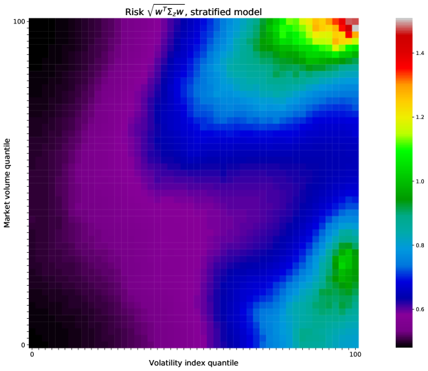
To visualize how the covariance varies with market conditions, we look at risk of a portfolio (i.e., the standard deviation of the return) with uniform allocation across the sectors. The risk is given by $\sqrt{w^{T}\Sigma w}$, where $\Sigma$ is the covariance matrix and $w=(1/9)\mathbf{1}$ is the weight vector corresponding to a uniform allocation. In figure 1, we plot the heatmap of the risk of this portfolio as a function of the market regime $z$ for the stratified model. The risk heatmap makes sense and varies smoothly across market conditions. The estimate of the risk of the uniform portfolio for the common model covariance matrix is $0.859$. The risk in our stratified model varies by about a factor of two from this common estimate of risk.

Figure 1: Heatmap of $\sqrt{w^{T}\Sigma_{z}w}$ with $w=(1/9)\mathbf{1}$ for the stratified model.

Application.

Here we demonstrate the use of our stratified risk model, in a simple trading policy. For each of the $K=2500$ market conditions, we compute the portfolio $w_{z}\in{\mbox{\bf R}}^{9}$ which is Markowitz optimal, i.e., the solution of

$$\begin{array}[]{ll}\mbox{maximize}&\mu^{T}w-\gamma w^{T}\Sigma_{z}w\\ \mbox{subject to}&\mathbf{1}^{T}w=1\\ &\|w\|_{1}\leq 2,\end{array}$$ (7)

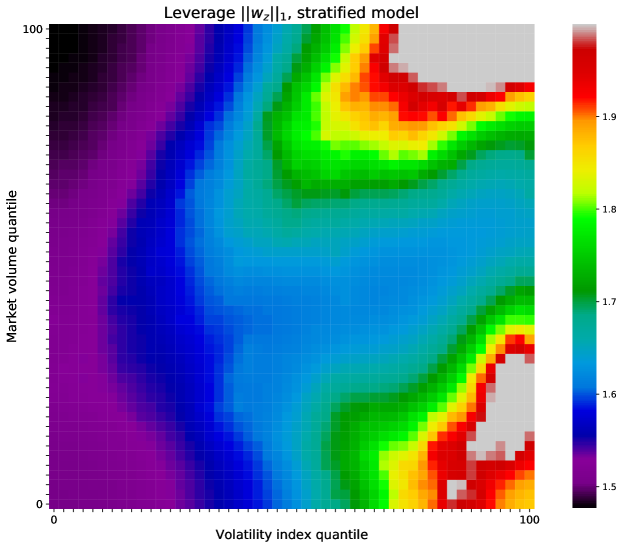
with optimization variable $w\in{\mbox{\bf R}}^{9}$ ($w_{i}<0$ denotes a short position in asset $i$). The objective is the risk adjusted return, and $\gamma>0$ is the risk-aversion parameter, which we take as $\gamma=0.15$. We take $\mu\in{\mbox{\bf R}}^{9}$ to be the vector of median sector returns in the training set. The last constraint limits the portfolio leverage, measured by $\|w\|_{1}$, to no more than 2. (This means that the total short positions in the portfolio cannot exceed $0.5$ times the total portfolio value.) We plot the leverage of the stratified model portfolios $w_{z}$, indexed by market conditions, in figure 2.

Figure 2: Heatmap of $\|w_{z}\|_{1}$, the stratified model portfolios, indexed by market conditions.

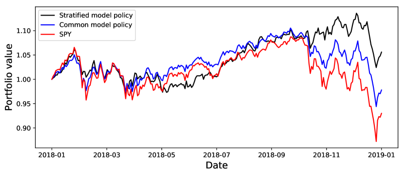
At the beginning of each day $t$, we use the previous day’s market conditions $z_{t}$ to allocate our current total portfolio value according to the weights $w_{z_{t}}$. We run this policy using realized returns from January 1, 2018 to January 1, 2019 (which was held out from all other previous experiments). In figure 3, we plot the cumulative value of three policies: Using the weights from the stratified model, using a constant weight from the common model, and simply buying and holding SPY.

Figure 3: Cumulative value of three portfolios, starting from initial value $1$.

In figure 4, we plot the sector weights of the stratified model policy and the weights of the common model policy.

Figure 4: Weights for the stratified model policy and the common policy over 2018.

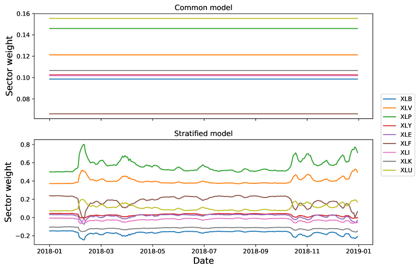
Table 2 gives the annualized realized risks and returns of the three policies. The stratified model policy has both the lowest annualized risk and the greatest annualized return. While the common model policy and buying and holding SPY realize losses over the year, our simple policy has a positive realized return.

Table 2: Annualized realized risks and returns for the three policies.

Model	Annualized risk	Annualized return
Stratified model	0.112	0.061
Common model	0.124	-0.015
Buy/hold SPY	0.170	-0.059

3.2 Space-time adaptive processing

In radar space time adaptive processing (STAP), a problem of widespread importance is the detection problem: detect a target over a terrain in the presence of interference. Interference typically comes in the form of clutter (unwanted terrain noise), jamming (noise emitted intentionally by an adversary), and white noise (typically caused by the circuitry/machinery of the radar receiver) [Mel04, WRAH06, Kan15]. (We refer to the sum of these three noises as interference.) In practice, these covariance matrices for a given radar orientation (i.e., for a given range, azimuth, Doppler frequency, etc.) are unknown and must be estimated [WRAH06, Kan15]. Our goal is to estimate the covariance matrix of the interference, given the radar orientation.

Data records.

Our data records $(z,y)$ include ground interference measurements $y\in{\mbox{\bf R}}^{30}$ (so $n=30$), which were synthetically generated (see below). In addition, the stratification features $z$ describe the radar orientation. A radar orientation corresponds to a tuple of the range $r$ (in km), azimuth angle $a$ (in degrees), and Doppler frequency $d$ (in Hz), which are binned. For example, if $z=(r,a,d)=([35,37),[87,89),[976,980))$, then the measurement was taken at a range between 35-57 km, an azimuth between 87-89 degrees, and a Doppler frequency between 976-980 Hz.

There are 10 range bins, 10 azimuth bins, and 10 Doppler frequency bins, and we allow $r\in[35,50]$, $a\in[87,267]$, and $d\in[-992,992]$; these radar orientation values are realistic and were selected from the radar signal processing literature; see [rad02, Table 1] and [Kan15, Table 3.1]. The number of stratification features is $K=10\cdot 10\cdot 10=1000$.

We generated the data records $(z,y)$ as follows. We generated three complex Hermitian matrices ${\widetilde{\Sigma}}_{\mathrm{range}}\in{\mbox{\bf C}}^{15}$, ${\widetilde{\Sigma}}_{\mathrm{azi}}\in{\mbox{\bf C}}^{15}$, and ${\widetilde{\Sigma}}_{\mathrm{dopp}}\in{\mbox{\bf C}}^{15}$ randomly, where C is the set of complex numbers. For each $z=(r,a,d)$, we generate a covariance matrix according to

$${\widetilde{\Sigma}}_{z}={\widetilde{\Sigma}}_{(r,a,d)}=\left(\frac{4\times 10^{4}}{r}\right)^{2}{\widetilde{\Sigma}}_{\mathrm{range}}+\left(\cos\left(\frac{\pi a}{180}\right)+\sin\left(\frac{\pi a}{180}\right)\right){\widetilde{\Sigma}}_{\mathrm{azi}}+\left(1+\frac{d}{1000}\right){\widetilde{\Sigma}}_{\mathrm{dopp}}.$$

For each $z$, we then independently sample from a Gaussian distribution with zero mean and covariance matrix ${\widetilde{\Sigma}}_{z}$ to generate the corresponding data samples $\widetilde{y}\in{\mbox{\bf R}}^{15}$. We then generate the real-valued data records $(z,y)$ from the complex-valued $(z,\widetilde{y})$ via $y=(\Re{\widetilde{y}},\Im{\widetilde{y}})$, where $\Re$ and $\Im$ denote the real and imaginary parts of $\widetilde{y}$, respectively, and equivalently estimate (the inverses of)

$$\Sigma_{z}=\begin{bmatrix}\Re{\widetilde{\Sigma}}_{z}&-\Im{\widetilde{\Sigma}}_{z}\\ \Im{\widetilde{\Sigma}}_{z}&\Re{\widetilde{\Sigma}}_{z}\\ \end{bmatrix},\quad z=1,\ldots,K,$$

the real-valued transformation of $\widetilde{\Sigma}_{z}$ [BV04, Ch. 4]. (Our model estimates the collection of real-valued natural parameters $\theta=(\Sigma^{-1}_{1},\ldots,\Sigma^{-1}_{K})$; it is trivial to obtain the equivalent collection of complex-valued natural parameters.) For the remainder of this section, we only consider the problem in its real-valued form.

We generate approximately 2900 samples and randomly partition the data set into 80% training samples and 20% test samples. The number of training samples per vertex vary significantly; there are a mean of 1.74 samples per vertex, and the maximum number of samples on a vertex is 30. 625 of the $K=1000$ vertices have no training samples associated with them.

Model.

The stratified model in this case is $K=1000$ (inverse) covariance matrices in ${\mbox{\bf S}}_{++}^{30}$, indexed by the radar orientation. Our model has $Kn(n-1)/2=435000$ parameters.

Regularization.

For local regularization, we utilize trace regularization with regularization weight $\gamma_{\mathrm{tr}}$, and $\ell_{1}$-regularization on the off-diagonal elements with regularization weight $\gamma_{\mathrm{od}}$. That is, $r(\theta)=\gamma_{\mathrm{tr}}\mathop{\bf Tr}(\theta)+\gamma_{\mathrm{od}}\|\theta\|_{\mathrm{od},1}$.

The regularization graph for the stratified model is taken as the Cartesian product of three regularization graphs:

• Range. The regularization graph is a path graph with 10 vertices, with edge weight $\gamma_{\mathrm{range}}$.

• Azimuth. The regularization graph is a cycle graph with 10 vertices, with edge weight $\gamma_{\mathrm{azi}}$.

• Doppler frequency. The regularization graph is a path graph with 10 vertices, with edge weight $\gamma_{\mathrm{dopp}}$.

The corresponding Laplacian matrix has 6600 nonzero entries and the hyper-parameters are $\gamma_{\mathrm{range}}$, $\gamma_{\mathrm{azi}}$, and $\gamma_{\mathrm{dopp}}$.

The stratified model in this case has five hyper-parameters: two for the local regularization, and three for the Laplacian regularization graph edge weights.

Results.

We compared a stratified model to a common model. The common model corresponds to solving one individual covariance estimation problem, ignoring the radar orientations. For the common model, we let $\gamma_{\mathrm{tr}}=0.001$ and $\gamma_{\mathrm{od}}=59.60$. For the stratified model, we let $\gamma_{\mathrm{tr}}=2.68$, $\gamma_{\mathrm{od}}=0.66$, $\gamma_{\mathrm{range}}=10.52$, $\gamma_{\mathrm{azi}}=34.30$, and $\gamma_{\mathrm{dopp}}=86.97$. These hyper-parameters were chosen by performing a crude hyper-parameter search and selecting hyper-parameters that performed well on the validation set. We compare the models’ average loss over the held-out test sets in table 3. In addition, we also compute the metric

$$D(\theta)=\frac{1}{Kn}\sum_{k=1}^{K}\left(\mathop{\bf Tr}(\Sigma_{k}^{\star}\theta_{k})-\log\det(\theta_{k})\right),$$

where $\Sigma_{k}^{\star}$ is the true covariance matrix for the stratification feature value $z=k$; this metric is used in the radar signal processing literature as a metric to determine how close $\theta_{k}^{-1}$ is to $\Sigma_{k}^{\star}$.

Table 3: Results for §3.2.

Model	Average test sample loss	$D(\theta)$
Common	0.153	2.02
Stratified	0.069	1.62

Application.

As another experiment, we consider utilizing these models in a target detection problem: given a vector of data $y\in{\mbox{\bf R}}^{30}$ and its radar orientation $z$, determine if the vector is just interference, i.e.,

$$y\mid z=d,\quad d\sim{\mathcal{N}}(0,\Sigma_{z}^{\star}),$$

or if the vector has some target associated with it, i.e.,

$$y\mid z=s_{z}+d,\quad d\sim{\mathcal{N}}(0,\Sigma_{z}^{\star})$$

for some target vector $s_{z}\in{\mbox{\bf R}}^{30}$, which is fixed for each $z$. (Typically, this is cast as a hypothesis test where the former is the null hypothesis and the latter is the alternative hypothesis [War95].) We generate $s_{z}$ with $z=(r,a,d)$ as

$$s_{z}=(\Re\widetilde{s}_{z},\Im\widetilde{s}_{z}),\qquad\widetilde{s}_{z}=(1,z_{d},z_{d}^{2})\otimes(1,z_{a},z_{a}^{2},z_{a}^{3},z_{a}^{4})$$

with $z_{a}=e^{2\pi i\sin(a)}$, $z_{d}=e^{2\pi id/f_{R}}$, and $f_{R}=1984$ is the pulse repetition frequency (in Hz); these values are realistic and selected from the radar signal processing literature [Kan15, Ch. 2]. For each $z$, we generate $y$ as follows: we sample a $d\sim{\mathcal{N}}(0,\Sigma_{z}^{\star})$, and with probability 1/2 we set $y=s_{z}+d$, and set $y=d$ otherwise. (There are 1000 samples). We then test if $y$ contains the target vector via the selection criterion

$$\frac{(s_{z}^{T}\theta_{z}y)^{2}}{s_{z}^{T}\theta_{z}s_{z}}>\alpha,$$

for some threshold $\alpha$; this is well-known in the radar signal processing literature as the optimal method for detection in this setting [RFKN92, WRAH06, Kan15]. If the selection criterion holds, then we classify $y$ as containing a target; otherwise, we classify $y$ as containing noise.

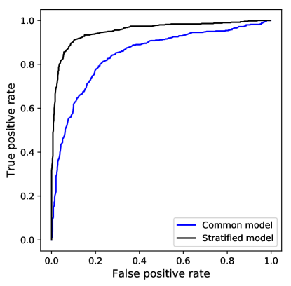
We vary $\alpha$ and test the samples on the common and stratified models. We plot the receiver operator characteristic (ROC) curves for both models in figure 5. The area under the ROC curve is 0.84 for the common model and 0.95 for the stratified model; the stratified model is significantly more capable at classifying in this setting.

Figure 5: ROC curves for the common and stratified models as the threshold $\alpha$ varies.

3.3 Temperature covariance estimation

We consider the problem of modeling the covariance matrix of hourly temperatures of a region as a function of day of year.

Data records and dataset.

We use temperature measurements (in Fahrenheit) from Boston, MA, sampled once per hour from October 2012 to October 2017, for a total of 44424 hourly measurements. We winsorize the data at its 1st and 99th percentiles. We then remove a baseline temperature, which consists of a constant and a sinusoid with period one year. We refer to this time series as the baseline-adjusted temperature.

From this data, we create data records $(z_{i},y_{i}),i=1,\ldots,1851$ (so $m=1851$), where $y_{i}\in{\mbox{\bf R}}^{24}$ is the baseline-adjusted temperature for day $i$, and $z_{i}\in\{1,\ldots,366\}$ is the day of the year. For example, $(y_{i})_{3}$ is the baseline-adjusted temperature at 3AM, and $z_{i}=72$ means that the day was the 72nd day of the year. The number of stratification features is then $K=366$, corresponding to the number of days in a year.

We randomly partition the dataset into a training set consisting of 60% of the data records, a validation set consisting of 20% of the data records, and a held-out test set consisting of the remaining 20% of the data records. In the training set, there are a mean of approximately 3.03 data records per day of year, the most populated vertex is associated with six data records, and there are seven vertices associated with zero data records.

Model.

The stratified model in this case is $K=366$ (inverse) covariance matrices in ${\mbox{\bf S}}_{++}^{24}$, indexed by the days of the year. Our model has $Kn(n-1)/2=101016$ parameters.

Regularization.

For local regularization, we utilize trace regularization with regularization weight $\gamma_{\mathrm{tr}}$, and $\ell_{1}$-regularization on the off-diagonal elements with regularization weight $\gamma_{\mathrm{od}}$. That is, $r(\theta)=\gamma_{\mathrm{tr}}\mathop{\bf Tr}(\theta)+\gamma_{\mathrm{od}}\|\theta\|_{\mathrm{od},1}$.

The stratification feature stratifies on day of year; our overall regularization graph, therefore, is a cycle graph with 366 vertices, one for each possible day of the year, with edge weights $\gamma_{\mathrm{day}}$. The associated Laplacian matrix contains 1096 nonzeros.

Results.

We compared a stratified model to a common model. The common model corresponds to solving one covariance estimation problem, ignoring the days of the year.

For the common model, we used $\gamma_{\mathrm{tr}}=359$ and $\gamma_{\mathrm{od}}=0.1$. For the stratified model, we used $\gamma_{\mathrm{tr}}=6000$, $\gamma_{\mathrm{od}}=0.1$, and $\gamma_{\mathrm{day}}=0.14$. These hyper-parameters were chosen by performing a crude hyper-parameter search and selecting hyper-parameters that performed well on the validation set.

We compare the models’ losses over the held-out test sets in table 4.

Table 4: Average loss over the test set for §3.3.

Model	Average test loss
Common	0.132
Stratified	0.093

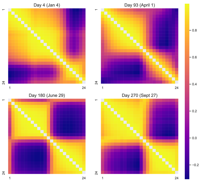
To illustrate some of these model parameters, in figure 6 we plot the heatmaps of the correlation matrices for days that roughly correspond to each season.

Figure 6: Heatmaps of the correlation matrices for days approximately corresponding to the start of winter (top left), spring (top right), summer (bottom left) and autumn (bottom right).

Application.

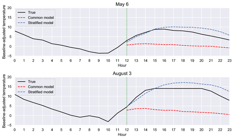
As another experiment, we consider the problem of forecasting the second half of a day’s baseline-adjusted temperature given the first half of the day’s baseline-adjusted temperature. We do this by modeling the baseline-adjusted temperature from the second half of the day as a Gaussian distribution conditioned on the observed baseline-adjusted temperatures [Mar84, Bis06]. We run this experiment using the common and stratified models found in the previous experiment, using the data in the held-out test set. In table 5, we compare the root-mean-square error (RMSE) between the predicted temperatures and the true temperatures over the held-out test set for the two models, and in figure 7, we plot the temperature forecasts for two days in the held-out test set.

Table 5: Average prediction RMSE over the test set for §3.3.

Model	Average prediction RMSE
Common	8.269
Stratified	6.091

Figure 7: Baseline-adjusted temperature forecasts for two days in the held-out test set.

References

- [AC00] R. Almgren and N. Chriss. Optimal execution of portfolio transactions. Journal of Risk, pages 5–39, 2000.
- [BBD+17] S. Boyd, E. Busseti, S. Diamond, R. N. Kahn, K. Koh, P. Nystrup, and J. Speth. Multi-period trading via convex optimization. Foundations and Trends in Optimization, 3(1):1–76, 2017.
- [BEGd08] O. Banerjee, L. El Ghaoui, and A. d’Aspremont. Model selection through sparse maximum likelihood estimation for multivariate Gaussian or binary data. Journal of Machine Learning Research, 9:485–516, 2008.
- [Bis06] C. M. Bishop. Pattern Recognition and Machine Learning. Springer, 2006.
- [BL08] P. J. Bickel and E. Levina. Covariance regularization by thresholding. The Annals of Statistics, 36(6):2577–2604, 12 2008.
- [BLW82] J. P. Burg, D. G. Luenberger, and D. L. Wenger. Estimation of structured covariance matrices. Proceedings of the IEEE, 70(9):963–974, Sep. 1982.
- [BPC+11] S. Boyd, N. Parikh, E. Chu, B. Peleato, and J. Eckstein. Distributed optimization and statistical learning via the alternating direction method of multipliers. Foundation and Trends in Machine Learning, 3(1):1–122, 2011.
- [BV04] S. Boyd and L. Vandenberghe. Convex Optimization. Cambridge University Press, 2004.
- [CB09] G. Cao and C. Bouman. Covariance estimation for high dimensional data vectors using the sparse matrix transform. In D. Koller, D. Schuurmans, Y. Bengio, and L. Bottou, editors, Advances in Neural Information Processing Systems 21, pages 225–232. Curran Associates, Inc., 2009.
- [DWW14] P. Danaher, P. Wang, and D. M. Witten. The joint graphical lasso for inverse covariance estimation across multiple classes. Journal of the Royal Statistical Society, 76(2):373–397, 2014.
- [Eng82] R. F. Engle. Autoregressive conditional heteroscedasticity with estimates of the variance of United Kingdom inflation. Econometrica, 50(4):987–1007, 1982.
- [Faz02] M. Fazel. Matrix Rank Minimization with Applications. PhD thesis, Stanford University, March 2002.
- [FHT08] J. Friedman, T. Hastie, and R. Tibshirani. Sparse inverse covariance estimation with the graphical lasso. Biostatistics, 9(3):432–441, 2008.
- [FLL16] J. Fan, Y. Liao, and H. Liu. An overview of the estimation of large covariance and precision matrices. The Econometrics Journal, 19(1):C1–C32, 2016.
- [GLMZ11] J. Guo, E. Levina, G. Michailidis, and J. Zhu. Joint estimation of multiple graphical models. Biometrika, 98(1):1–15, February 2011.
- [HL96] J. P. Hoffbeck and D. A. Landgrebe. Covariance matrix estimation and classification with limited training data. IEEE Transactions on Pattern Analysis and Machine Intelligence, 18(7):763–767, July 1996.
- [HLB15] D. Hallac, J. Leskovec, and S. Boyd. Network lasso: Clustering and optimization in large graphs. In Proceedings of the ACM International Conference on Knowledge Discovery and Data Mining, pages 387–396, 2015.
- [HPBL17] D. Hallac, Y. Park, S. Boyd, and J. Leskovec. Network inference via the time-varying graphical lasso. In Proceedings of the ACM International Conference on Knowledge Discovery and Data Mining, pages 205–213, 2017.
- [HS52] M. Hestenes and E. Stiefel. Methods of conjugate gradients for solving linear systems. Journal of Research of the National Bureau of Standards, 49(6), 1952.
- [Kan15] B. Kang. Robust Covariance Matrix Estimation for Radar Space-Time Adaptive Processing (STAP). PhD thesis, The Pennsylvania State University, August 2015.
- [KF09] D. Koller and N. Friedman. Probabilistic Graphical Models: Principles and Techniques. The MIT Press, 2009.
- [KOSZ13] J. A. Kelner, L. Orecchia, A. Sidford, and Z. A. Zhu. A simple, combinatorial algorithm for solving sdd systems in nearly-linear time. In Proceedings of the Forty-Fifth Annual ACM Symposium on Theory of Computing, STOC ’13, page 911–920, New York, NY, USA, 2013. Association for Computing Machinery.
- [KVM+99] W. Kernan, C. Viscoli, R. Makuch, L. Brass, and R. Horwitz. Stratified randomization for clinical trials. Journal of clinical epidemiology, 52(1):19–26, 1999.
- [LH87] E. Levitan and G. T. Herman. A maximum a posteriori probability expectation maximization algorithm for image reconstruction in emission tomography. IEEE Transactions on Medical Imaging, 6(3):185–192, Sept 1987.
- [LSL99] H. Li, P. Stoica, and J. Li. Computationally efficient maximum likelihood estimation of structured covariance matrices. IEEE Transactions on Signal Processing, 47(5):1314–1323, May 1999.
- [Mar52] H. Markowitz. Portfolio selection. The Journal of Finance, 7(1):77–91, 1952.
- [Mar84] F. H. C. Marriott. Multivariate Statistics: A Vector Space Approach. Journal of the Royal Statistical Society Series C, 33(3):319–319, November 1984.
- [Mel04] W. L. Melvin. A STAP overview. IEEE Aerospace and Electronic Systems Magazine, 19(1):19–35, Jan 2004.
- [MM16] J. Ma and G. Michailidis. Joint structural estimation of multiple graphical models. Journal of Machine Learning Research, 17(166):1–48, 2016.
- [MS87] M. I. Miller and D. L. Snyder. The role of likelihood and entropy in incomplete-data problems: Applications to estimating point-process intensities and toeplitz constrained covariances. Proceedings of the IEEE, 75(7):892–907, July 1987.
- [PB14] N. Parikh and S. Boyd. Proximal algorithms. Foundations and Trends in Optimization, 1(3):127–239, 2014.
- [rad02] High-fidelity site-specific radar data set. In Knowledge-Aided Sensor Signal Processing & Expert Reasoning Workshop 2002, April 2002.
- [RFKN92] F. C. Robey, D. R. Fuhrmann, E. J. Kelly, and R. Nitzberg. A CFAR adaptive matched filter detector. IEEE Transactions on Aerospace and Electronic Systems, 28(1):208–216, 1992.
- [RFP10] B. Recht, M. Fazel, and P. A. Parrilo. Guaranteed minimum-rank solutions of linear matrix equations via nuclear norm minimization. SIAM Review, 52(3):471–501, August 2010.
- [SB09] J. Skaf and S. Boyd. Multi-period portfolio optimization with constraints and transaction costs, 2009.
- [SBP17] Y. Sun, P. Babu, and D. Palomar. Majorization-minimization algorithms in signal processing, communications, and machine learning. IEEE Transactions in Signal Processing, 65(3):794–816, 2017.
- [SCC+19] S. Salari, F. Chan, Y. Chan, I. Kim, and R. Cormier. Joint DOA and clutter covariance matrix estimation in compressive sensing MIMO radar. IEEE Transactions on Aerospace and Electronic Systems, 55(1):318–331, Feb 2019.
- [SG00] M. Steiner and K. Gerlach. Fast converging adaptive processor or a structured covariance matrix. IEEE Transactions on Aerospace and Electronic Systems, 36(4):1115–1126, Oct 2000.
- [TB20] J. Tuck and S. Boyd. Eigen-stratified models, 2020.
- [TBB19] J Tuck, S. Barratt, and S. Boyd. A Distributed Method for Fitting Laplacian Regularized Stratified Models. arXiv e-prints, page arXiv:1904.12017, Apr 2019.
- [THB19] J. Tuck, D. Hallac, and S. Boyd. Distributed majorization-minimization for Laplacian regularized problems. IEEE/CAA Journal of Automatica Sinica, 6(1):45–52, January 2019.
- [TJ16] R. Takapoui and H. Javadi. Preconditioning via diagonal scaling, 2016.
- [VB96] L. Vandenberghe and S. Boyd. Semidefinite programming. SIAM Review, 38(1):49–95, 1996.
- [Vis13] N. Vishnoi. Lx= b. Foundations and Trends in Theoretical Computer Science, 8(1–2):1–141, 2013.
- [War95] J. Ward. Space-time adaptive processing for airborne radar. In 1995 International Conference on Acoustics, Speech, and Signal Processing, volume 5, pages 2809–2812, 1995.
- [WBAW12] B. Wahlberg, S. Boyd, M. Annergren, and Y. Wang. An ADMM algorithm for a class of total variation regularized estimation problems. In 16th IFAC Symposium on System Identification, 2012.
- [WRAH06] M. C. Wicks, M. Rangaswamy, R. Adve, and T. B. Hale. Space-time adaptive processing: a knowledge-based perspective for airborne radar. IEEE Signal Processing Magazine, 23(1):51–65, Jan 2006.
- [WT09] D. M. Witten and R. Tibshirani. Covariance-regularized regression and classification for high dimensional problems. Journal of the Royal Statistical Society, 71(3):615–636, 2009.
- [ZSP14] Y. Zhu, X. Shen, and W. Pan. Structural pursuit over multiple undirected graphs. Journal of the American Statistical Association, 109(508):1683–1696, 2014.