Identification of Self-Excited Systems Using Discrete-Time, Time-Delayed Lur’e Models

Abstract

This paper presents a system identification technique for systems whose output is asymptotically periodic under constant inputs. The model used for system identification is a discrete-time Lur’e model consisting of asymptotically stable linear dynamics, a time delay, a washout filter, and a static nonlinear feedback mapping. For all sufficiently large scalings of the loop transfer function, these components cause divergence under small signal levels and decay under large signal amplitudes, thus producing an asymptotically oscillatory output. A bias-generation mechanism is used to provide a bias in the oscillation. The contribution of the paper is a least-squares technique that estimates the coefficients of the linear model as well as the parameterization of the continuous, piecewise-linear feedback mapping.

1 Introduction

Nonlinear system identification is an exciting area of research with numerous challenges and open problems; the overview in Schoukens  Ljung (2019) describes the status of the field and provides extensive references. The present paper focuses on nonlinear system identification for systems whose response to a constant input is asymptotically periodic; a system of this type is called a self-excited system (SES). A classical example of a SES is the van der Pol oscillator, whose states converge to a limit cycle. A SES, however, may have an arbitrary number of states and need not possess a limit cycle. Overviews of SES are given in Jenkins (2013); Ding (2010); applications to chemical and biochemical systems are discussed in Chance . (1973); Gray  Scott (1990); Goldbeter  Berridge (1996); self-excited thermoacoustic oscillation is discussed in Dowling (1997); Awad  Culick (1986); Chen  Driscoll (2016); and fluid-structure interaction and its role in aircraft wing flutter is discussed in Blevins (1990); Friedmann (1999); Coller  Chamara (2004); Jonsson . (2019).

A convenient model for SES is a feedback loop consisting of linear dynamics and a static nonlinear feedback mapping; a system of this type is called a Lur’e system Khalil (2002). Within the context of SES, Lur’e systems are considered in Ding (2010); Jian  Yu-shu (2004); Zanette (2017); Risau-Gusman (2016); Chatterjee (2011); Stan  Sepulchre (2007); Tomberg  Yakubovich (1989); Mees  Chua (1979); Aguilar . (2009); Hang . (2002); Stan  Sepulchre (2004); Savaresi . (2001). Self-oscillating discrete-time systems are considered in Rasvan (1998); D’Amico . (2002, 2004); Gentile . (2011).

As discussed in Paredes, Islam, Kouba  Bernstein (2020); Paredes, Islam  Bernstein (2020), self-excited oscillations arise in Lur’e systems from a combination of stabilizing and destabilizing effects. Destabilization at small signal levels causes the output to diverge, whereas stabilization at large signal levels causes the output to decay.

To provide a framework for SES system identification, this paper considers a discrete-time, time-delay Lur’e model consisting of an asymptotically stable linear system, a time delay, a washout filter, and a static nonlinear feedback mapping. For all sufficiently large scalings of the loop transfer function, these components cause divergence under small signal levels and decay under large signal amplitudes, thus producing an asymptotically oscillatory output. A bias-generation mechanism is used to provide a nonzero offset in the oscillation. Similar features appear in Jian  Yu-shu (2004); Zanette (2017); Risau-Gusman (2016); Ding (2010); Chatterjee (2011). Conditions under which the Lur’e model used in the present paper is SES are given in Paredes, Islam, Kouba  Bernstein (2020); Paredes, Islam  Bernstein (2020).

The contribution of the present paper is the development of a technique for identifying SES using discrete-time, time-delayed Lur’e models. In setting up the model structure, the user must choose the order of the linear discrete-time model and the number of steps delay. Once these are chosen, the system identification method estimates the parameters of the linear discrete-time model as well as the static nonlinear feedback mapping, which is formulated as a continuous, piecewise-linear (CPL) function characterized by its slope in each interval of a user-chosen partition of the real line. Although a nonlinear least-squares optimization technique can be used for parameter estimation, we adopt the approach of Van Pelt  Bernstein (2001); Van Pelt  Bernstein (2000), which minimizes a bound on the least-square cost function that can be optimized by linear least squares.

The contents of the paper are as follows. Section 2 introduces SES and the DTTDL model used for identification. Section 3 describes the parameterization of the CPL functions used to approximate the nonlinear feedback mapping. Section 4 presents the DTTDL/CPL model, which consists of the DTTDL model with the CPL mapping parameterized in Section 3. Section 5 describes the least-squares technique for identifying SES using CTTDL/CPL, and Section 6 describes a variation of this technique for the constant-input case. Section 7 presents numerical examples.

Notation. ${\mathbb{R}}\stackrel{{\scriptstyle\triangle}}{{=}}(-\infty,\infty),$ $\mathbb{N}\stackrel{{\scriptstyle\triangle}}{{=}}\{0,1,2,\ldots\}.$

2 Identification of self-excited systems using discrete-time, time-delayed Lur’e models

Let ${\mathcal{S}}$ be a discrete-time, self-excited system (SES) with input $v$ and output $y,$ and let ${\mathcal{M}}$ be a discrete-time model with input $v$ and output $y_{\rm m}$ (see Figure 1). The signals $v,y,y_{\rm m}$ are scalar. The structure of ${\mathcal{M}}$ is designed to capture the self-excited dynamics of ${\mathcal{S}}$ in the sense that, for all sufficiently large constant $v,$ there exist a nonconstant periodic function $\tau\colon{\mathbb{N}}\to{\mathbb{R}}$ and $k_{0}\in\BBN$ such that $\lim_{k\to\infty}|y_{k}-\tau_{k}|=0$ and $\lim_{k\to\infty}|y_{{\rm m},k}-\tau_{k+k_{0}}|=0.$ In the case where ${\mathcal{S}}$ is a continuous-time SES, the output $y_{k}$ represents a sampled value of $y(t).$ In this paper, ${\mathcal{M}}$ is chosen to be a discrete-time, time-delayed Lur’e model.

Figure 1: Self-excited system ${\mathcal{S}}$ with input $v$ and output $y,$ and model ${\mathcal{M}}$ with input $v$ and output $y_{\rm m}.$ A system identification algorithm is used to construct a model ${\mathcal{M}}$ that captures the dynamics of ${\mathcal{S}}$.

The discrete-time, time-delayed Lur’e (DTTDL) model shown in Figure 2 incorporates the $n$th-order, asymptotically stable, strictly proper linear system

$$G({\bf q})=\frac{B({\bf q})}{A({\bf q})}=\frac{b_{1}{\bf q}^{n-1}+\cdots+b_{n}}{{\bf q}^{n}+a_{1}{\bf q}^{n-1}+\cdots+a_{n}},$$ (1)

where ${\bf q}$ is the forward-shift operator, the bias-generation mechanism

$$v_{\rm b}=(\beta+v_{\rm f})v,$$ (2)

the time delay $G_{\rm d}({\bf q})={\bf q}^{-d}$, where $d\geq 0,$ the washout filter

$$G_{\rm f}({\bf q})=\frac{{\bf q}-1}{{\bf q}},$$ (3)

and the nonlinear function ${\mathcal{N}}\colon{\mathbb{R}}\to{\mathbb{R}}$ written as

$$v_{{\rm f},k}={\mathcal{N}}(y_{{\rm f},k}).$$ (4)

Using $y_{{\rm m},k}=G({\bf q})v_{{\rm b},k},$ it follows that

$$A({\bf q})y_{{\rm m},k} =B({\bf q})v_{{\rm b},k}$$

$$=B({\bf q})[\beta+{\mathcal{N}}(y_{{\rm f},k})]v_{k},$$ (5)

and thus, for all $k\geq n+d+1,$

$$y_{{\rm m},k} =(1-A({\bf q}))y_{{\rm m},k}+B({\bf q})[\beta+{\mathcal{N}}(y_{{\rm f},k})]v_{k}$$

$$=-a_{1}y_{{\rm m},k-1}-\cdots-a_{n}y_{{\rm m},k-n}+\beta(b_{1}v_{k-1}+\cdots+b_{n}v_{k-n})$$

$$\quad+b_{1}{\mathcal{N}}(y_{{\rm f},k-1})v_{k-1}+\cdots+b_{n}{\mathcal{N}}(y_{{\rm f},k-n})v_{k-n},$$ (6)

where

$$y_{{\rm f},k}=y_{{\rm m},k-d}-y_{{\rm m},k-d-1}.$$

Note that the propagation of (6) depends on the initial output values $y_{{\rm m},0},\ldots,y_{{\rm m},n+d}.$

In Paredes, Islam, Kouba  Bernstein (2020); Paredes, Islam  Bernstein (2020), ${\mathcal{N}}$ is assumed to be bounded, continuous, either nondecreasing or nonincreasing, and changes sign (positive to negative or vice versa) at zero; hence, ${\mathcal{N}}(0)=0$. Under these assumptions, it is shown in Paredes, Islam, Kouba  Bernstein (2020); Paredes, Islam  Bernstein (2020) that, if the input $v$ is constant and sufficiently large, then the output $y_{\rm m}$ is nonconstant and asymptotically periodic.

Figure 2: Discrete-time, time-delayed Lur’e model with constant input $v$ and bias-generation mechanism.

3 Parameterization of the continuous, piecewise-linear function ${\mathcal{N}}$

In this section, we assume that ${\mathcal{N}}$ is continuous and piecewise-linear (CPL), and we parameterize ${\mathcal{N}}$ as in Van Pelt  Bernstein (2001). Let $c_{1}<\cdots<c_{p}$, let $(-\infty,c_{1}],(c_{1},c_{2}],\ldots,(c_{p-1},c_{p}],(c_{p},\infty)$ be a partition of the domain ${\mathbb{R}}$ of ${\mathcal{N}},$ and define the vector

$$c\stackrel{{\scriptstyle\triangle}}{{=}}{[\begin{array}[]{ccc}c_{1}&\cdots&c_{p}\end{array}]}^{\rm T}\in{\mathbb{R}}^{p}.$$ (7)

Furthermore, for all $i=1,\ldots,p+1,$ let $\mu_{i}$ denote the slope of ${\mathcal{N}}$ in the $i$th partition interval, and define the slope vector

$$\mu\stackrel{{\scriptstyle\triangle}}{{=}}{[\begin{array}[]{ccc}\mu_{1}&\cdots&\mu_{p+1}\end{array}]}^{\rm T}\in{\mathbb{R}}^{p+1}.$$ (8)

Finally, letting $\kappa\in{\mathbb{R}}$ and $r\in\{1,\ldots,p\},$ it follows that, for all $u\in{\mathbb{R}},$ ${\mathcal{N}}$ can be written as

$${\mathcal{N}}(u)=\mu^{\rm T}\eta(u)+\kappa,$$ (9)

where $\eta\colon{\mathbb{R}}\to{\mathbb{R}}^{p+1}$ is defined by

$$\eta(u)\stackrel{{\scriptstyle\triangle}}{{=}}\begin{cases}\eta_{1}(u),&\delta(u)<r+1,\\ \eta_{2}(u),&\delta(u)\geq r+1,\end{cases}$$ (10)

$\delta(u)\in\{1,\ldots,p+1\}$ is the index of the partition interval containing $u$, and

$$\eta_{1}(u) \stackrel{{\scriptstyle\triangle}}{{=}}{[\begin{array}[]{cccccc}0_{1\times(\delta(u)-1)}&u-c_{\delta(u)}&c_{\delta(u)}-c_{\delta(u)+1}&\cdots&c_{r-1}-c_{r}&0_{1\times(p+1-r)}\end{array}]}^{\rm T},$$ (12)

$$\eta_{2}(u) \stackrel{{\scriptstyle\triangle}}{{=}}{[\begin{array}[]{cccccc}0_{1\times r}&c_{r+1}-c_{r}&\cdots&c_{\delta(u)-1}-c_{\delta(u)-2}&u-c_{\delta(u)-1}&0_{1\times(p+1-\delta(u))}\end{array}]}^{\rm T}.$$ (14)

Note that, if $\delta(u)=r,$ then $\eta_{1}(u)={[\begin{array}[]{cccccc}0_{1\times(\delta(u)-1)}&u-c_{\delta(u)}&0_{1\times(p+1-r)}\end{array}]}^{\rm T},$ whereas, if $\delta(u)=r+1,$ then $\eta_{2}(u)\stackrel{{\scriptstyle\triangle}}{{=}}{[\begin{array}[]{cccccc}0_{1\times r}&u-c_{\delta(u)-1}&0_{1\times(p+1-\delta(u))}\end{array}]}^{\rm T}.$ Since ${\mathcal{N}}(c_{r})=\kappa,$ it can be seen that $r$ and $\kappa$ fix ${\mathcal{N}}$ along the ordinate axis, as shown in Figure 3. Hence, ${\mathcal{N}}$ is parameterized by $c,$ $\mu,$ $r,$ and $\kappa.$

Figure 3: Parameterization of the CPL function ${\mathcal{N}}.$ Note that $r$ and $\kappa$ fix $g$ along the ordinate axis.

4 DTTDL model with a CPL nonlinear feedback mapping

In this section, we consider the DTTDL model in the case where ${\mathcal{N}}$ is CPL; this is the DTTDL/CPL model. In order to enforce ${\mathcal{N}}(0)=0$ (see Section 2), we let $\kappa=0$ and assume that, for some $r,$ $c_{r}=0.$ It thus follows from (6) and (9) that

$$y_{{\rm m},k} =-a_{1}y_{{\rm m},k-1}-\cdots-a_{n}y_{{\rm m},k-n}$$

$$\quad+\beta(b_{1}v_{k-1}+\cdots+b_{n}v_{k-n})$$

$$\quad+b_{1}\mu^{\rm T}\eta(y_{{\rm f},k-1})v_{k-1}+\cdots+b_{n}\mu^{\rm T}\eta(y_{{\rm f},k-n})v_{k-n}.$$ (15)

Now, defining

$$a\stackrel{{\scriptstyle\triangle}}{{=}}{[\begin{array}[]{ccc}a_{1}&\cdots&a_{n}\end{array}]}^{\rm T},\quad b\stackrel{{\scriptstyle\triangle}}{{=}}{[\begin{array}[]{ccc}b_{1}&\cdots&b_{n}\end{array}]}^{\rm T},$$ (18)

it follows that (15) can be written as

$$y_{{\rm m},k}=\phi_{k}^{\rm T}\theta,$$ (19)

where

$$\theta\stackrel{{\scriptstyle\triangle}}{{=}}\left[\begin{array}[]{c}a\\ {\rm vec}(\mu b^{\rm T})\\ \beta b\end{array}\right],$$ (20)

$$\phi_{k}\stackrel{{\scriptstyle\triangle}}{{=}}{[\begin{array}[]{ccc}-\phi_{y,k}^{\rm T}&\phi_{\eta,k}^{\rm T}&\phi_{v,k}^{\rm T}\end{array}]}^{\rm T},$$ (21)

and

$$\phi_{y,k} \stackrel{{\scriptstyle\triangle}}{{=}}{[\begin{array}[]{ccc}y_{{\rm m},k-1}&\cdots&y_{{\rm m},k-n}\end{array}]}^{\rm T},$$ (23)

$$\phi_{\eta,k} \stackrel{{\scriptstyle\triangle}}{{=}}{[\begin{array}[]{ccc}v_{k-1}{\eta}^{\rm T}(y_{{\rm f},k-1})&\cdots&v_{k-n}{\eta}^{\rm T}(y_{{\rm f},k-n})\end{array}]}^{\rm T},$$ (25)

$$\phi_{v,k} \stackrel{{\scriptstyle\triangle}}{{=}}{[\begin{array}[]{ccc}v_{k-1}&\cdots&v_{k-n}\end{array}]}^{\rm T}.$$ (27)

5 Identification of DTTDL/CPL model parameters

In this section, we present a least-squares identification technique for constructing a DTTDL/CPL model that approximates the response of the self-excited system ${\mathcal{S}}$. Since we do not assume that ${\mathcal{S}}$ is a DTTDL system, the goal is to determine asymptotically stable $\hat{G}$ and CPL $\hat{\mathcal{N}}$ such that the response of the identified model ${\mathcal{M}}$ approximates the response of the true system ${\mathcal{S}}.$

The least-squares identification technique depends on choosing values of $n,d,c$; these choices are denoted by $\hat{n},\hat{d},\hat{c}$. In practice, $\hat{n},\hat{d},\hat{c}$ can be iteratively modified depending on the accuracy of the identification. The goal is thus to obtain parameter estimates $\hat{a},\hat{b},\hat{\beta},\hat{\mu}$ for the DTTDL/CPL model. In the special case where ${\mathcal{S}}$ is DTTDL or DTTDL/CPL, the parameters $\hat{a},\hat{b},\hat{\beta},\hat{\mu}$ can be viewed as estimates of $a,b,\beta,\mu$.

Next, let $l_{\rm u}\geq l_{\rm l}\geq\hat{n}+\hat{d}+1$ and, for all $k\in\{l_{\rm l}-\hat{n}-\hat{d}-1,\ldots,l_{\rm u}\},$ let $v_{k}$ and $y_{k}$ be the sampled measurements of ${\mathcal{S}}$ used for identification. Then, define the least-squares cost

$$J(\theta)\stackrel{{\scriptstyle\triangle}}{{=}}{||Y-\Phi\theta||}_{2},$$ (28)

where

$$Y\stackrel{{\scriptstyle\triangle}}{{=}}{[\begin{array}[]{ccc}y_{l_{\rm l}}&\cdots&y_{l_{\rm u}}\end{array}]}^{\rm T},$$ (29)

and

$$\Phi\stackrel{{\scriptstyle\triangle}}{{=}}[\begin{array}[]{ccc}-\Phi_{Y}&\Phi_{\eta,Y}&\Phi_{\rm V}\end{array}],$$ (30)

where

$$\Phi_{Y}\stackrel{{\scriptstyle\triangle}}{{=}}\left[\begin{array}[]{c}\phi_{Y,l_{\rm l}}^{\rm T}\\ \vdots\\ \phi_{Y,l_{\rm u}}^{\rm T}\end{array}\right],\hskip 22.76219pt\Phi_{\eta,Y}\stackrel{{\scriptstyle\triangle}}{{=}}\left[\begin{array}[]{c}\phi_{\eta,Y,l_{\rm l}}^{\rm T}\\ \vdots\\ \phi_{\eta,Y,l_{\rm u}}^{\rm T}\end{array}\right],\hskip 22.76219pt\Phi_{{\rm V}}\stackrel{{\scriptstyle\triangle}}{{=}}\left[\begin{array}[]{c}\phi_{v,l_{\rm l}}^{\rm T}\\ \vdots\\ \phi_{v,l_{\rm u}}^{\rm T}\end{array}\right],$$ (31)

and

$$\phi_{Y,k} \stackrel{{\scriptstyle\triangle}}{{=}}{[\begin{array}[]{ccc}y_{k-1}&\cdots&y_{k-\hat{n}}\end{array}]}^{\rm T},$$ (33)

$$\phi_{\eta,Y,k} \stackrel{{\scriptstyle\triangle}}{{=}}{[\begin{array}[]{ccc}v_{k-1}{\eta}^{\rm T}(y_{{\rm f},Y,k-1})&\cdots&v_{k-\hat{n}}{\eta}^{\rm T}(y_{{\rm f},Y,k-\hat{n}})\end{array}]}^{\rm T},$$ (35)

$$y_{{\rm f},Y,k} \stackrel{{\scriptstyle\triangle}}{{=}}y_{k-\hat{d}}-y_{k-\hat{d}-1}.$$ (36)

Since $\theta$ given by (20) is not linear in $b,\mu,\beta,$ we derive an upper bound for $J(\theta),$ which is subsequently minimized. To do this, let $\theta_{\mathcal{A}}\in{\mathbb{R}}^{n(p+1)},$ define $\theta_{\Lambda}\stackrel{{\scriptstyle\triangle}}{{=}}\beta b,$ and note that (29) can be written as

$$J(\theta) ={||Y-\Phi\theta+\Phi_{\eta,Y}\theta_{\mathcal{A}}-\Phi_{\eta,Y}\theta_{\mathcal{A}}||}_{2}$$

$$={||Y+\Phi_{Y}a-\Phi_{\eta,Y}{\rm vec}(\mu b^{\rm T})-\Phi_{{\rm V}}\theta_{\Lambda}+\Phi_{\eta,Y}\theta_{\mathcal{A}}-\Phi_{\eta,Y}\theta_{\mathcal{A}}||}_{2}$$

$$={||Y-\Phi\tilde{\theta}+\Phi_{\eta,Y}(\theta_{\mathcal{A}}-{\rm vec}(\mu b^{\rm T}))||}_{2},$$ (37)

where

$$\tilde{\theta}\stackrel{{\scriptstyle\triangle}}{{=}}\left[\begin{array}[]{c}a\\ \theta_{\mathcal{A}}\\ \theta_{\Lambda}\end{array}\right].$$ (38)

It follows from (37) that

$$J(\theta) \leq{||Y-\Phi\tilde{\theta}||}_{2}+{||\Phi_{\eta,Y}(\theta_{\mathcal{A}}-{\rm vec}(\mu b^{\rm T}))||}_{2}$$

$$\leq{||Y-\Phi\tilde{\theta}||}_{2}+\sigma_{\rm max}(\Phi_{\eta,Y}){||\theta_{\mathcal{A}}-{\rm vec}(\mu b^{\rm T})||}_{2}$$

$$=J_{\rm LS}(\tilde{\theta})+\sigma_{\rm max}(\Phi_{\eta,Y})J_{\mathcal{A}}(\theta_{\mathcal{A}},\mu,b),$$ (39)

where

$$J_{\rm LS}(\tilde{\theta})\stackrel{{\scriptstyle\triangle}}{{=}}{||Y-\Phi\tilde{\theta}||}_{2},$$ (40)

$$J_{\mathcal{A}}(\theta_{\mathcal{A}},\mu,b)\stackrel{{\scriptstyle\triangle}}{{=}}{||{\rm vec}^{-1}(\theta_{\mathcal{A}})-\mu b^{\rm T}||}_{\rm F},$$ (41)

${||\cdot||}_{\rm F}$ denotes the Frobenius norm, and $\sigma_{\rm max}$ denotes the largest singular value.

The upper bound for $J(\theta)$ given by (39) is minimized by sequentially minimizing $J_{\rm LS}(\bar{\theta})$ and $J_{\mathcal{A}}(\theta_{\mathcal{A}},\mu,b)$ to obtain

$$\hat{\tilde{\theta}}\stackrel{{\scriptstyle\triangle}}{{=}}\underset{\bar{\theta}_{0}\in{\mathbb{R}}^{n(p+3)}}{\rm argmin}\,J_{\rm LS}(\bar{\theta}_{0})=\left[\begin{array}[]{c}\hat{a}\\ \hat{\theta}_{\mathcal{A}}\\ \hat{\theta}_{\Lambda}\end{array}\right],$$ (42)

where $\hat{\theta}_{\mathcal{A}}\in{\mathbb{R}}^{n(p+1)}$ and $\hat{\theta}_{\Lambda}\stackrel{{\scriptstyle\triangle}}{{=}}\hat{\beta}\hat{b}.$ Note that $\hat{\tilde{\theta}}$ can be obtained by applying linear least-squares minimization to $J_{\rm LS}.$ Since $\hat{\beta}$ and $\hat{b}$ are unidentifiable from $\hat{\theta}_{\Lambda},$ choosing an arbitrary nonzero value for $\hat{\beta}$ yields $\hat{b}=\hat{\theta}_{\Lambda}/\hat{\beta}.$

The following result is used to obtain $\hat{\mu}=\underset{\mu_{0}\in{\mathbb{R}}^{p+1}}{\rm argmin}\,J_{\mathcal{A}}(\hat{\theta}_{\mathcal{A}},\mu_{0},\hat{b}).$

Proposition 5.1.

Let $A\in{\mathbb{R}}^{n\times m}$, let $r\in{\mathbb{R}}^{m}$ be nonzero, and define $V\colon{\mathbb{R}}^{n}\to{\mathbb{R}}$ by

$$V(x)\stackrel{{\scriptstyle\triangle}}{{=}}{||A-xr^{\rm T}||}_{\rm F}^{2}.$$ (43)

$$\underset{x\in{\mathbb{R}}^{n}}{\rm argmin}\,V(x)=(r^{\rm T}r)^{-1}{Ar}.$$ (44)

Proof. For all $x\in{\mathbb{R}}^{n},$

$$V(x)={\rm tr}(A^{\rm T}A)-2x^{\rm T}Ar+x^{\rm T}xr^{\rm T}r,$$ (45)

and thus

$$V^{\prime}(x)=-2Ar+2r^{\rm T}rx,$$ (46)

$$V^{\prime\prime}(x)=2r^{\rm T}r>0.$$ (47)

It follows from (47) and (Bazaraa ., 2006, Theorem 3.3.8, p. 115) that $V$ is strictly convex, which implies that $V$ has at most one minimizer. Since

$$V^{\prime}((r^{\rm T}r)^{-1}{Ar})=0,$$ (48)

(47) implies that $(r^{\rm T}r)^{-1}{Ar}$ is a local minimizer of $V$. Hence, (Bazaraa ., 2006, Theorem 3.4.2, pp. 125, 126) implies that $(r^{\rm T}r)^{-1}{Ar}$ is the unique minimizer of $V.$ $\hfill\square$

Proposition 5.1 implies that, for fixed $\hat{\theta}_{\mathcal{A}}$ and $\hat{b},$ the value of $\hat{\mu}$ that minimizes $\hat{\mu}\mapsto J_{\mathcal{A}}(\hat{\theta}_{\mathcal{A}},\hat{\mu},\hat{b})$ is given by

$$\hat{\mu}=\frac{{\rm vec}^{-1}(\hat{\theta}_{\mathcal{A}})\hat{b}}{\hat{b}^{\rm T}\hat{b}}.$$ (49)

The identified DTTDL/CPL model ${\mathcal{M}}$ is characterized by the chosen parameters $\hat{n},\hat{d},\hat{c},\hat{\beta},$ as well as the estimated parameters $\hat{a},\hat{b},\hat{\mu}.$ Note that multiplying $\hat{\beta}$ by nonzero $\gamma\in{\mathbb{R}}$ results in the division of $\hat{b}$ by $\gamma$ and the multiplication of $\hat{\mu}$ by $\gamma$, which modifies the estimate of the nonlinear feedback mapping. However, it follows from (15) that the response of the identified model remains unchanged.

6 Identification of DTTDL/CPL model parameters with constant input

This section considers a variation of the identification technique presented in the previous section for the case where $v$ is constant, as typically occurs in self-excited systems. For $v_{k}\equiv v_{0}$, (15) becomes

$$y_{{\rm m},k} =-a_{1}y_{{\rm m},k-1}-\cdots-a_{n}y_{{\rm m},k-n}+\beta v_{0}(b_{1}+\cdots+b_{n})$$

$$\quad+v_{0}[b_{1}\mu^{\rm T}\eta(y_{{\rm f},k-1})+\cdots+b_{n}\mu^{\rm T}\eta(y_{{\rm f},k-n})].$$ (50)

Then, (50) can be expressed as (19), where

$$\theta\stackrel{{\scriptstyle\triangle}}{{=}}\left[\begin{array}[]{c}a\\ {\rm vec}(\mu b^{\rm T})\\ \beta 1_{1\times n}b\end{array}\right],$$ (54)

$$\phi_{k}\stackrel{{\scriptstyle\triangle}}{{=}}{[\begin{array}[]{ccc}-\phi_{y,k}^{\rm T}&\phi_{\eta,k}^{\rm T}&v_{0}\end{array}]}^{\rm T},$$ (56)

$\phi_{y,k}$ is defined by (23), and where

$$\phi_{\eta,k} \stackrel{{\scriptstyle\triangle}}{{=}}v_{0}\ {[\begin{array}[]{ccc}{\eta}^{\rm T}(y_{{\rm f},k-1})&\cdots&{\eta}^{\rm T}(y_{{\rm f},k-n})\end{array}]}^{\rm T}.$$ (58)

Furthermore, $J(\theta)$ can be written as in (28), where $Y$ is defined by (29) and $\Phi$ is defined by (30)–(36), where

$$\Phi_{{\rm V}} \stackrel{{\scriptstyle\triangle}}{{=}}v_{0}1_{(l_{\rm u}-l_{\rm l}+1)\times 1},$$ (59)

$$\phi_{\eta,Y,k} \stackrel{{\scriptstyle\triangle}}{{=}}v_{0}{[\begin{array}[]{ccc}{\eta}^{\rm T}(y_{{\rm f},Y,k-1})&\cdots&{\eta}^{\rm T}(y_{{\rm f},Y,k-\hat{n}})\end{array}]}^{\rm T}.$$ (61)

Since $\theta$ given by (54) is not linear in $b,\mu,\beta,$ we derive an upper bound for $J(\theta),$ which is subsequently minimized. Next, (28) can be rewritten as in (37), where $\theta_{\mathcal{A}}\in{\mathbb{R}}^{n(p+1)},$ $\theta_{\Lambda}\stackrel{{\scriptstyle\triangle}}{{=}}\beta 1_{1\times n}b,$ and $\tilde{\theta}$ is defined as in (38). Then, an upper bound for $J(\theta)$ can be derived as in $\eqref{Jineq2},$ where $J_{\rm LS}$ and $J_{\mathcal{A}}$ are defined as in (40) and (41), and can be minimized by sequentially minimizing $J_{\rm LS}(\bar{\theta})$ and $J_{\mathcal{A}}(\theta_{\mathcal{A}},\mu,b).$ Let $\hat{\theta}_{\mathcal{A}}\in{\mathbb{R}}^{n(p+1)},$ define $\hat{\theta}_{\Lambda}\stackrel{{\scriptstyle\triangle}}{{=}}\hat{\beta}1_{1\times n}\hat{b},$ and define $\hat{\bar{\theta}}$ as in (42). Then $\hat{\bar{\theta}}$ can be obtained by minimizing $J_{\rm LS}.$

Next, (Bernstein, 2018, Fact 11.16.39, p. 906) implies that, for fixed $\hat{\theta}_{\mathcal{A}},$ the rank-1 approximation of $\hat{\mu}\hat{b}^{\rm T}$ that minimizes $J_{\mathcal{A}}(\hat{\theta}_{\mathcal{A}},\hat{\mu},\hat{b})$ is given by

$$\hat{\mu}\hat{b}^{\rm T}=\sigma_{\rm max}({\rm vec}^{-1}(\hat{\theta}_{\mathcal{A}}))u_{{\mathcal{A}},1}v_{{\mathcal{A}},1}^{\rm T},$$ (62)

where $\sigma_{\rm max}$ denotes the largest singular value, $u_{{\mathcal{A}},1}$ denotes the first left-singular vector of ${\rm vec}^{-1}(\hat{\theta}_{\mathcal{A}}),$ and $v_{{\mathcal{A}},1}$ denotes the first right-singular vector of ${\rm vec}^{-1}(\hat{\theta}_{\mathcal{A}}).$ Since $\hat{\mu}$ and $\hat{b}$ are unidentifiable from (62), choosing arbitrary nonzero $\beta_{\rm LS}\in{\mathbb{R}}$ and using it to separate (62) yields

$$\hat{\mu}=\beta_{\rm LS}\ \sigma_{\rm max}({\rm vec}^{-1}(\hat{\theta}_{\mathcal{A}}))u_{{\mathcal{A}},1},\hskip 14.22636pt\hat{b}=\frac{v_{{\mathcal{A}},1}}{\beta_{\rm LS}}.$$ (63)

Finally, $\hat{\beta}$ is given by

$$\hat{\beta}=\frac{\hat{\theta}_{\Lambda}}{1_{1\times\hat{n}}\hat{b}}.$$ (64)

The identified DTTDL/CPL model ${\mathcal{M}}$ is characterized by the chosen parameters $\hat{n},\hat{d},\beta_{\rm LS},$ and $\hat{c},$ as well as the estimated parameters $\hat{a},\hat{b},$ $\hat{\beta}$ and $\hat{\mu}.$ Note that multiplying $\beta_{\rm LS}$ by nonzero $\gamma\in{\mathbb{R}}$ results in the division of $\hat{b}$ by $\gamma,$ and the multiplication of $\hat{\mu}$ (which scales $\hat{\mathcal{N}}$) and $\hat{\beta}$ by $\gamma.$ However, it follows from (15) that the response of the identified model remains unchanged.

7 Numerical examples

In this section, we present numerical examples to illustrate identification of DTTDL/CPL models. Recursive least squares (RLS) is used for regression, as presented in Astrom  Wittenmark (1995); Islam  Bernstein (2019). Table 1 summarizes the details of the numerical examples considered in this section. The identified systems include three DTTDL systems, one continuous-time, time-delayed Lur’e (CTTDL) system, the Van der Pol (VdP) system with output bias, and the predator-prey Lotka-Volterra system. For continuous-time systems, $T_{\rm d}$ is the time delay. For examples 7 to 7, it is assumed that the input $v$ is known. However, since examples 7 and 7 do not involve an external input, an arbitrary value of the input $v$ is used to facilitate identification of the DTTDL model. Note that the outputs of the systems in Example 7.2 and Example 7.3 are asymptotically periodic under sufficiently large constant inputs, despite the fact that the nonlinearities in these systems do not satisfy the assumptions on ${\mathcal{N}}$ in Section 2.

Table 1: Examples for DTTDL/CPL System Identification

Example	System Type	$\bm{n}$	$\bm{d}$	$T_{{\rm d}}$	$\bm{{\mathcal{N}}}$	Parameters
7	DTTDL	2	4	n/a	CPL, monotonic, odd	$\beta=7.5$
7	DTTDL	3	4	n/a	C${}^{\infty},$ monotonic, not odd	$\beta=5$
7	DTTDL	6	0	n/a	C${}^{\infty},$ not monotonic, odd	$\beta=2.5$
7	CTTDL	2	n/a	0.1 s	C${}^{\infty},$ monotonic, odd	$\beta=50,$ $T_{\rm s}=0.1$ s
7	VdP w/bias	2	n/a	n/a	C${}^{\infty},$ multivariable	$\mu_{0}=1,$ $\overline{y}=10,$ $T_{\rm s}=0.1$ s
7	Lotka-Volterra	n/a	n/a	n/a	n/a	$\zeta=2/3,\varrho=4/3,$ $\xi=1,\varphi=1,$ $T_{\rm s}=0.1$ s

Example 7: DTTDL system with CPL, monotonic, odd ${\mathcal{N}}$

Consider the DTTDL system ${\mathcal{S}}$ with $\beta=7.5,$ $d=4,$

$$G({\bf q})=\frac{{\bf q}-0.5}{{\bf q}^{2}-1.6{\bf q}+0.8},$$ (65)

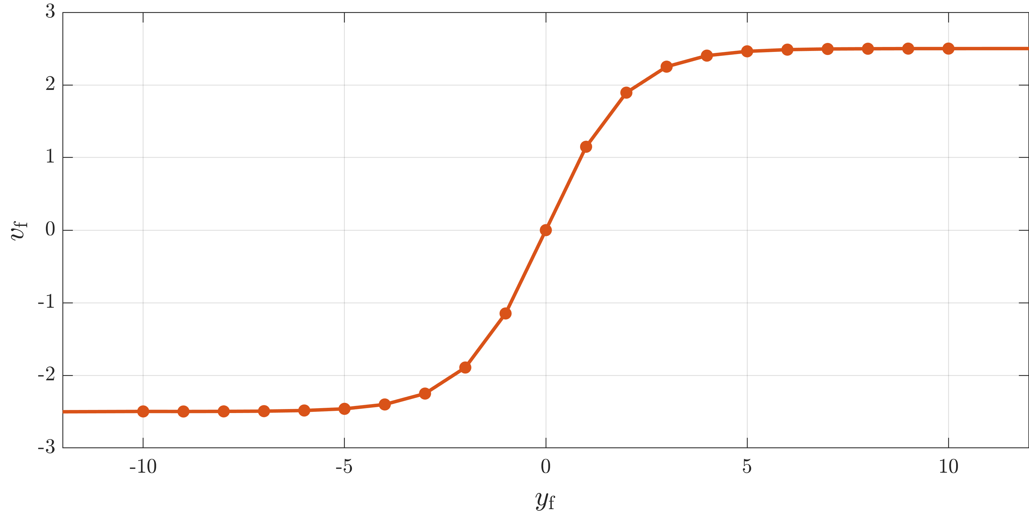
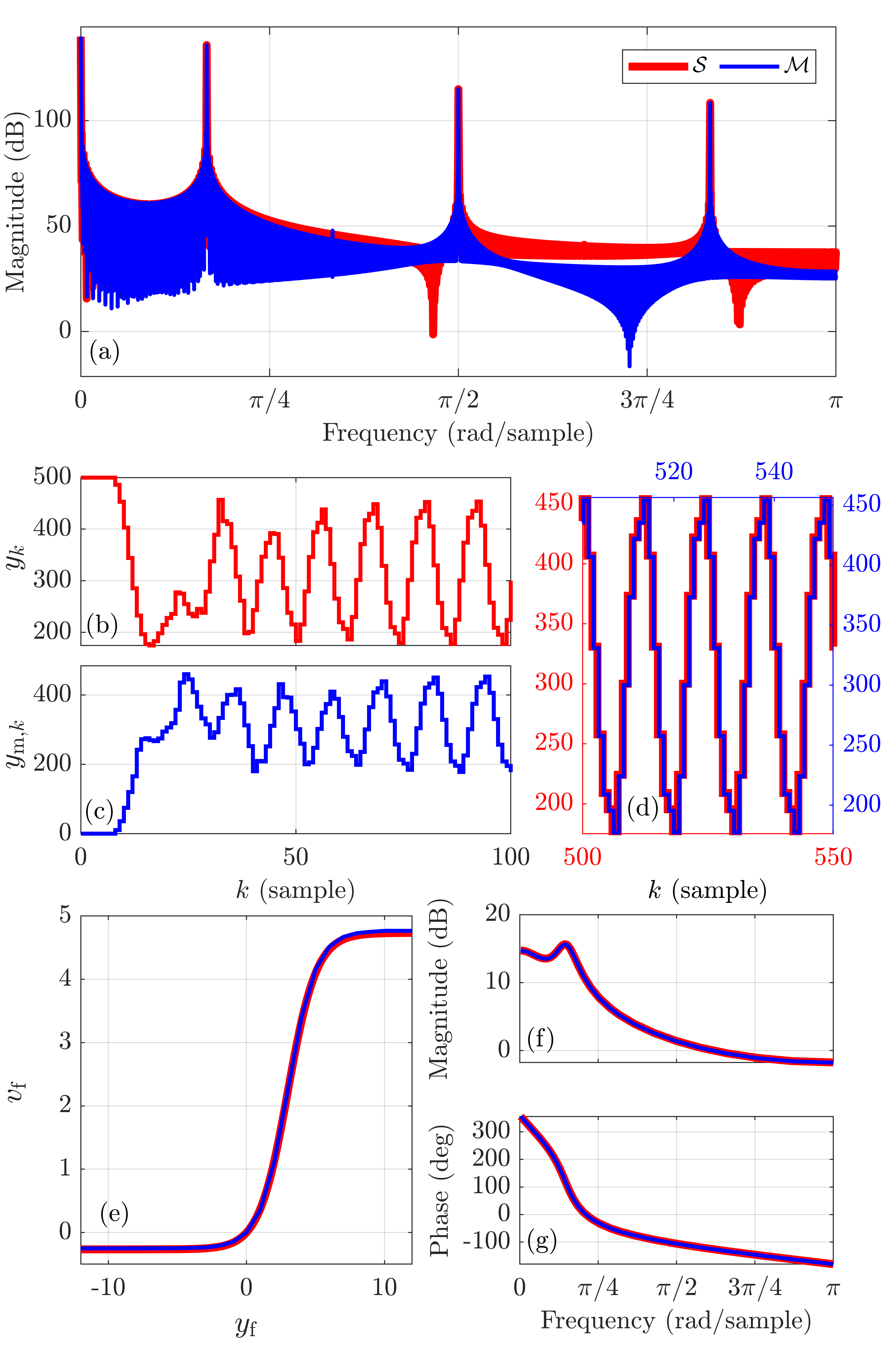
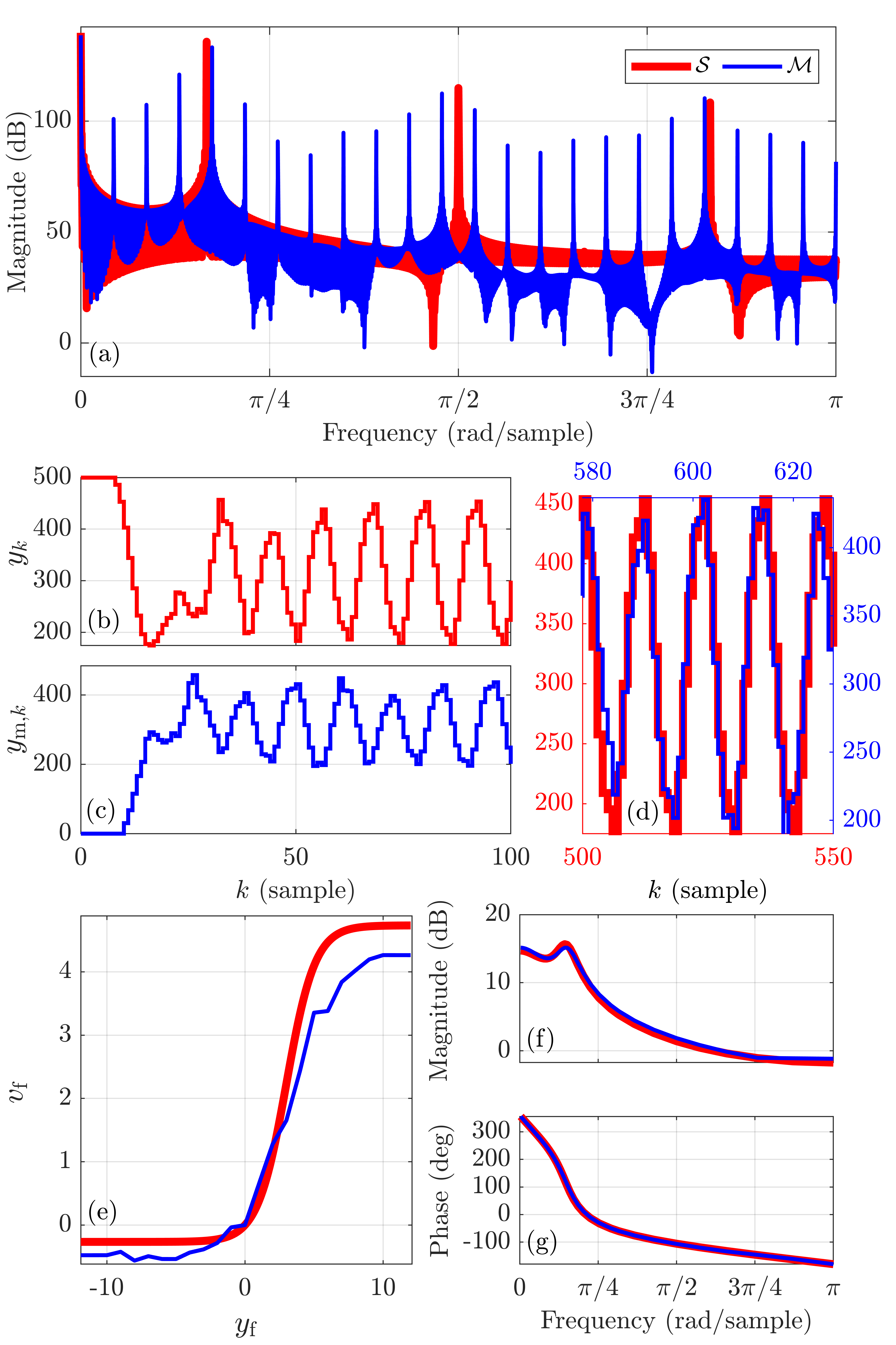
and the CPL, monotonic, odd feedback mapping ${\mathcal{N}}$ shown in Figure 4. The domain of ${\mathcal{N}}$ is partitioned by $c={[\begin{array}[]{ccccccc}-10&-9&\cdots&9&10\end{array}]}^{\rm T},$ and ${\mathcal{N}}$ is constructed such that, for all $i\in\{1,\ldots,21\},$ ${\mathcal{N}}(c_{i})=2.5\tanh(1.2c_{i}/2.5).$ To obtain data for identification, $y_{0},\ldots,y_{6}$ are generated randomly, and, for all $k\geq 0,$ $v_{k}$ is a gaussian random variable with mean $5$ and standard deviation $\sqrt{1.5}.$ For all $k\geq 7,$ $y_{k}$ is generated by simulating ${\mathcal{S}}$ with (65). The same technique is used in all subsequent examples.

For least-squares identification of the DTTDL/CPL model parameters, we let $\hat{c}=c$ and $\hat{\beta}=\beta$, and we apply RLS with $\theta_{0}=0,$ $P_{0}={10}^{6}$ and $\lambda=1$ using data in $[100,25000].$ The standard deviation of the sensor noise is chosen to be $\sqrt{1.5},$ which yields a measurement signal-to-noise ratio (SNR) of approximately $40$ dB.

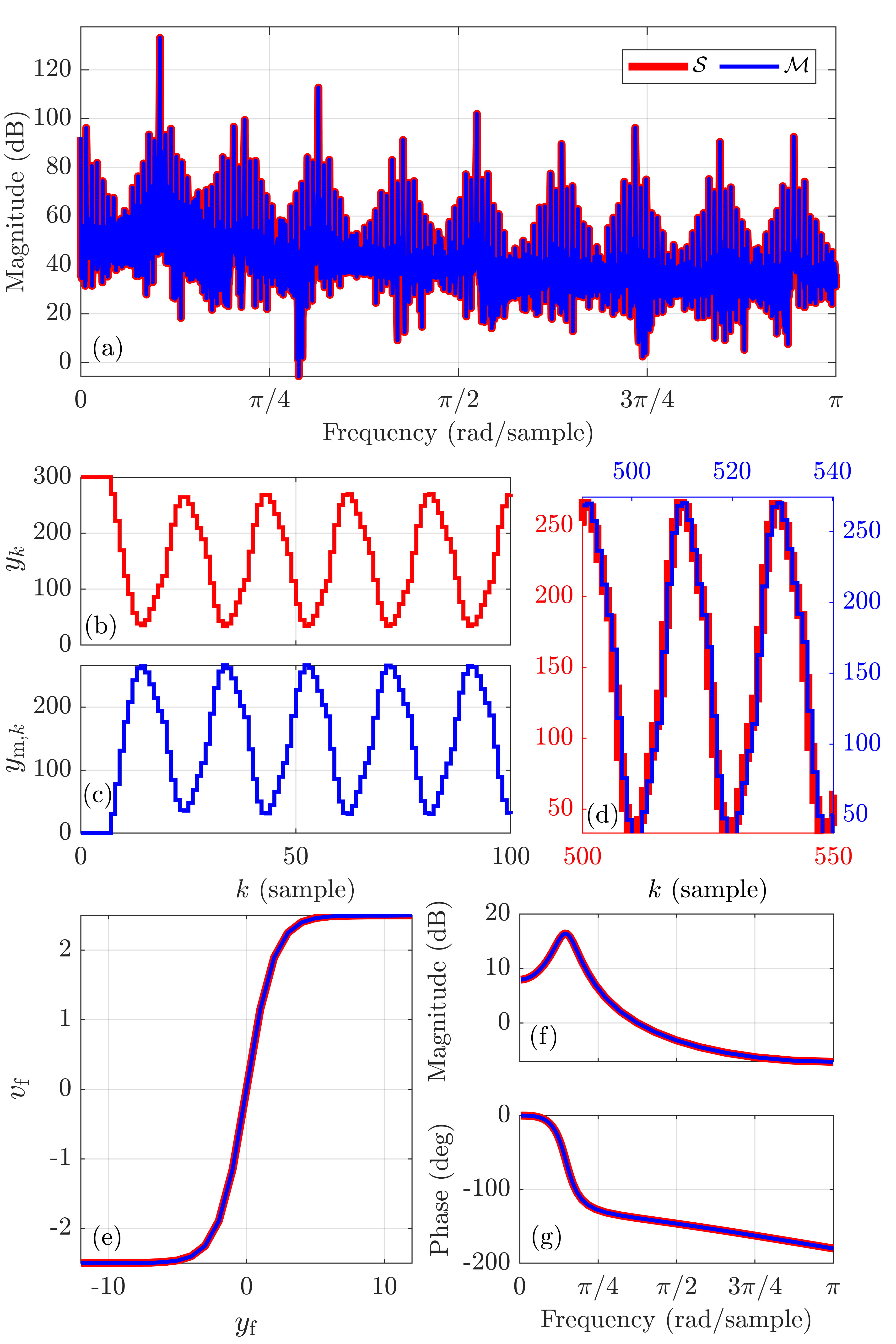
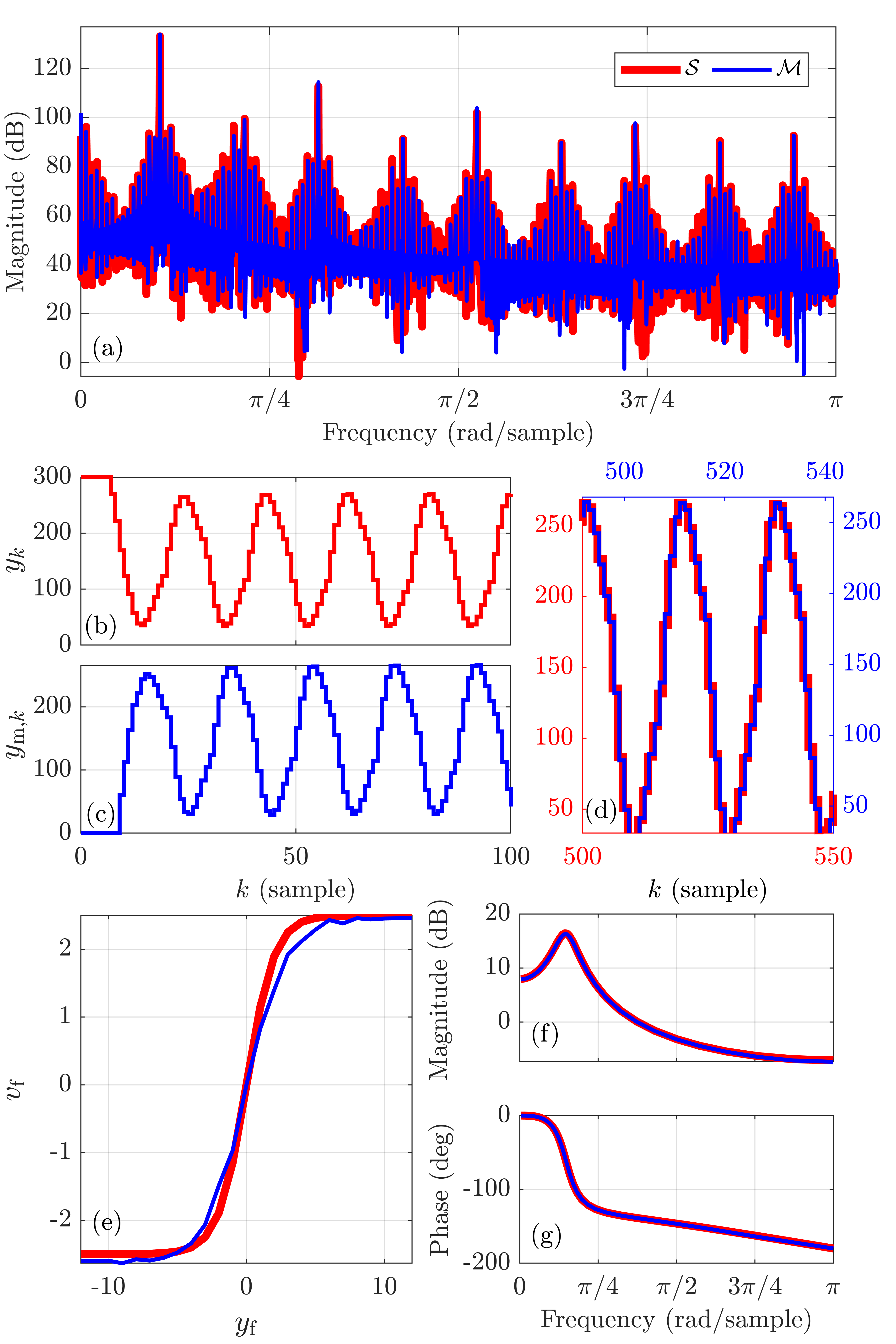
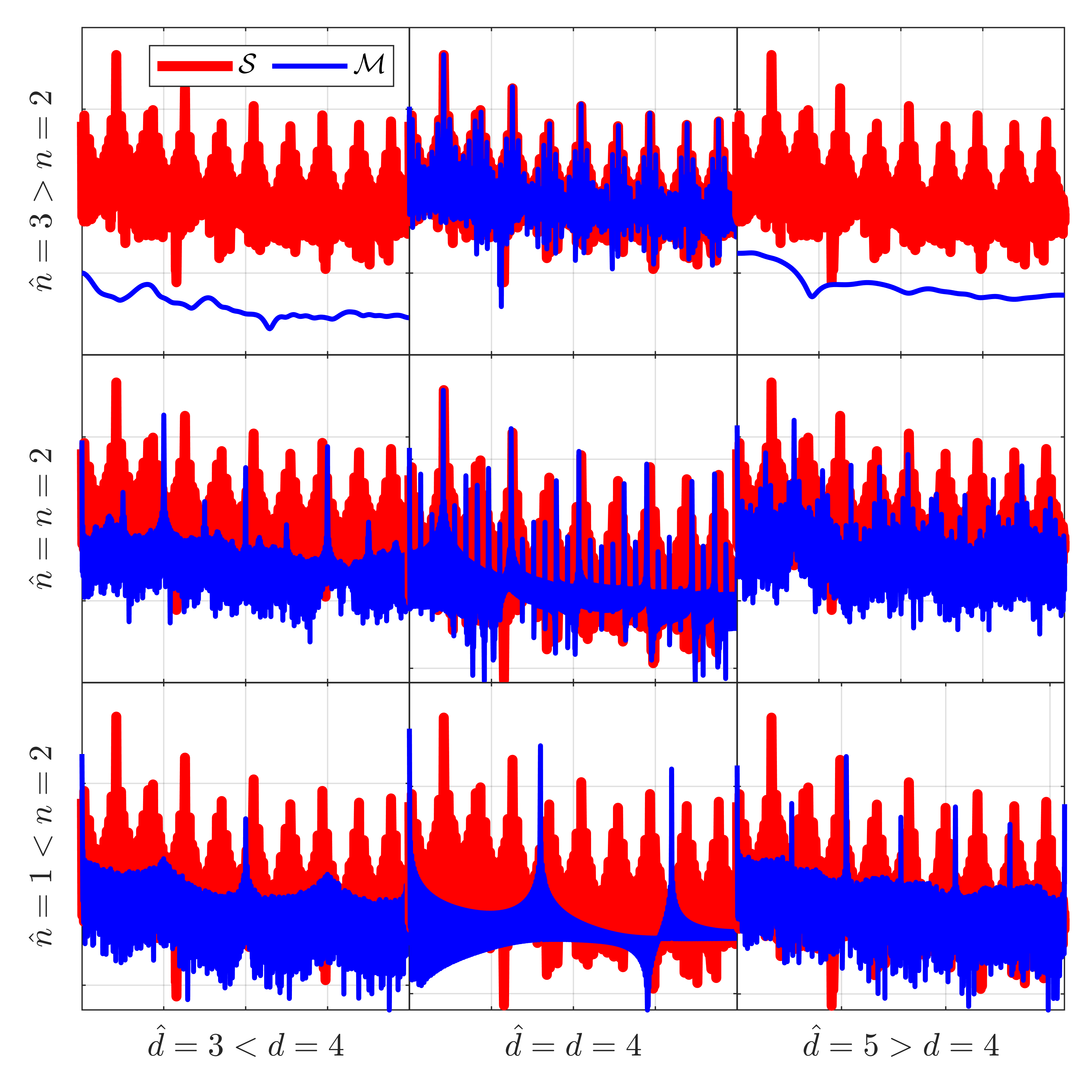
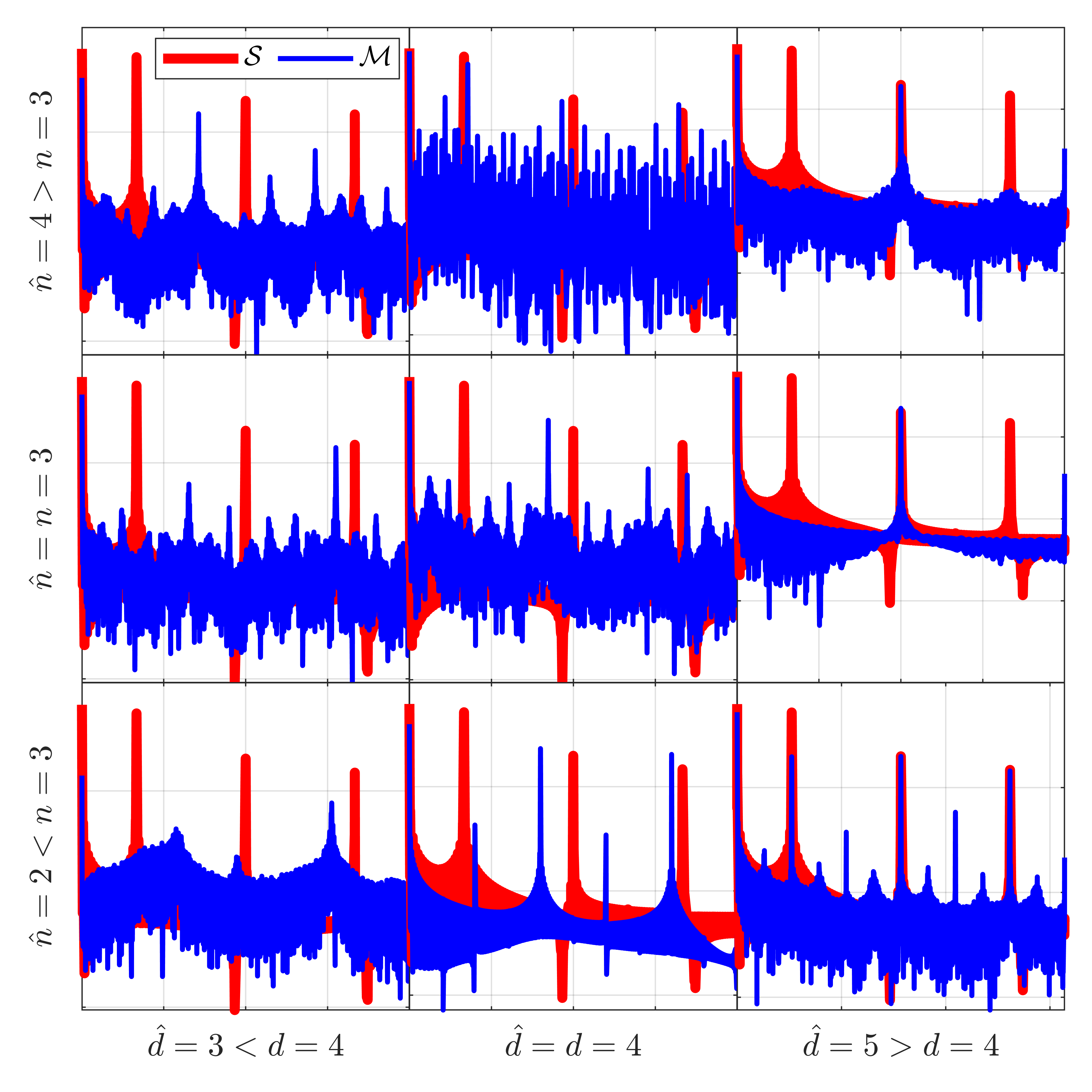
To assess the accuracy of the identified model, the input $v_{k}\equiv 8$ is applied to the system ${\mathcal{S}}$ with the initial conditions $y_{k}=300$ for all $k\in[0,6],$ as well as the identified model ${\mathcal{M}}$ with the initial conditions $y_{{\rm m},k}=0$ for all $k\in[0,6].$ The response of the identified model based on noiseless measurements with $\hat{n}=n$ and $\hat{d}=d$ is shown in Figure 5, and the response of the identified model based on noisy measurements with $\hat{n}=4$ and $\hat{d}=d$ is shown in Figure 6. Figure 7 compares the power spectral density (PSD) of the output of ${\mathcal{M}}$ for $\hat{n}\in\{1,2,3\}$ and $\hat{d}\in\{3,4,5\}$ obtained using noisy measurements with the PSD of the output of ${\mathcal{S}}$.

Figure 4: Example 7: Piecewise-linear feedback mapping ${\mathcal{N}}$.

Figure 5: Example 7: Least-squares identification of DTTDL/CPL model parameters using noiseless measurements with $\hat{n}=n$ and $\hat{d}=d.$ (a) compares the power spectral density (PSD) of the output of ${\mathcal{M}}$ with the PSD of the output of ${\mathcal{S}}$. (b) shows the output of ${\mathcal{S}}$ with $v_{k}\equiv 8$ and with $y_{k}=300$ for all $k\in[0,6]$. (c) shows the output of ${\mathcal{M}}$ with $v_{k}\equiv 8$ and with $y_{{\rm m},k}=0$ for all $k\in[0,6]$. (d) shows the output of ${\mathcal{S}}$ on $[500,550]$ and the output of ${\mathcal{M}}$ on $[491,540].$ (e) shows the true and estimated nonlinearities. (f) and (g) show the frequency responses of the linear dynamics of ${\mathcal{S}}$ and ${\mathcal{M}}$.

Figure 6: Example 7: Least-squares identification of DTTDL/CPL model parameters using noisy measurements for $\hat{n}=4$ and $\hat{d}=d.$ (a) compares the PSD of the output of ${\mathcal{M}}$ with the PSD of the output of ${\mathcal{S}}$. (b) shows the output of ${\mathcal{S}}$ with $v_{k}\equiv 8$ and with $y_{k}=300$ for all $k\in[0,6]$. (c) shows the output of ${\mathcal{M}}$ with $v_{k}\equiv 8$ and with $y_{{\rm m},k}=0$ for all $k\in[0,6]$. (d) shows the output of ${\mathcal{S}}$ on $[500,550]$ and the output of ${\mathcal{M}}$ on $[492,541]$. (e) shows the true and estimated nonlinearities. (f) and (g) show the frequency responses of the linear dynamics of ${\mathcal{S}}$ and ${\mathcal{M}}$.

Figure 7: Example 7: For $\hat{n}\in\{1,2,3\}$ and $\hat{d}\in\{3,4,5\}$, these plots compare the PSD of the output of ${\mathcal{M}}$ identified using noisy measurements with the PSD of the output of ${\mathcal{S}}$.

Example 7: DTTDL system with $C^{\infty},$ monotonic, not odd ${\mathcal{N}}$

Consider the DTTDL system ${\mathcal{S}}$ with $\beta=5,$ $d=4,$

$$G({\bf q})=\frac{{\bf q}^{2}-2.3{\bf q}-1.5725}{{\bf q}^{3}-2.35{\bf q}^{2}+2{\bf q}-0.6},$$ (66)

and ${\mathcal{N}}(y_{\rm f})=2.5\tanh\left(1.2(y_{\rm f}-3)/2.5\right)+2.2342,$ which is monotonic but not odd. To obtain data for identification, $y_{0},\ldots,y_{7}$ are generated randomly, and, for all $k\geq 0,$ $v_{k}$ is a gaussian random variable with mean 4 and standard deviation $\sqrt{2}.$ For all $k\geq 8,$ $y_{k}$ is generated by simulating ${\mathcal{S}}$ with (66).

For least-squares identification of the DTTDL/CPL model parameters, we let $\hat{c}={[\begin{array}[]{ccccccc}-10&-9&\ldots&9&10\end{array}]}^{\rm T}$ and $\hat{\beta}=\beta,$ and we apply RLS with $\theta_{0}=0,$ $P_{0}={10}^{6}$ and $\lambda=1$ using data in $[100,25000].$ The standard deviation of the sensor noise is chosen to be $\sqrt{2.65}$, which yields a measurement SNR of approximately $40$ dB.

To assess the accuracy of the identified model, the input $v_{k}\equiv 8$ is applied to the system ${\mathcal{S}}$ with the initial conditions $y_{k}=500$ for all $k\in[0,7],$ as well as the identified model ${\mathcal{M}}$ with the initial conditions $y_{{\rm m},k}=0$ for all $k\in[0,7].$ The response of the identified model based on noiseless measurements with $\hat{n}=n$ and $\hat{d}=d$ is shown in Figure 8, and the response of the identified model based on noisy measurements with $\hat{n}=5$ and $\hat{d}=d$ is shown in Figure 9. Figure 10 compares the PSD of the output of ${\mathcal{M}}$ for $\hat{n}\in\{2,3,4\}$ and $\hat{d}\in\{3,4,5\}$ obtained using noisy measurements with the PSD of the output of ${\mathcal{S}}$.

Figure 8: Example 7: Least-squares identification of DTTDL/CPL model parameters using noiseless measurements with $\hat{n}=n$ and $\hat{d}=d.$ (a) compares the PSD of the output of ${\mathcal{M}}$ with the PSD of the output of ${\mathcal{S}}$. (b) shows the output of ${\mathcal{S}}$ with $v_{k}\equiv 8$ and with $y_{k}=500$ for all $k\in[0,7]$. (c) shows the output of ${\mathcal{M}}$ with $v_{k}\equiv 8$ and with $y_{{\rm m},k}=0$ for all $k\in[0,7]$. (d) shows the output of ${\mathcal{S}}$ on $[500,550]$ and the output of ${\mathcal{M}}$ on $[502,552].$ (e) shows the true and estimated nonlinearities. (f) and (g) show the frequency responses of the linear dynamics of ${\mathcal{S}}$ and ${\mathcal{M}}$.

Figure 9: Example 7: Least-squares identification of DTTDL/CPL model parameters using noisy measurements for $\hat{n}=5$ and $\hat{d}=d.$ (a) compares the PSD of the output of ${\mathcal{M}}$ with the PSD of the output of ${\mathcal{S}}$. (b) shows the output of ${\mathcal{S}}$ with $v_{k}\equiv 8$ and with $y_{k}=500$ for all $k\in[0,7]$. (c) shows the output of ${\mathcal{M}}$ with $v_{k}\equiv 8$ and with $y_{{\rm m},k}=0$ for all $k\in[0,7]$. (d) shows the output of ${\mathcal{S}}$ on $[500,550]$ and the output of ${\mathcal{M}}$ on $[579,629].$ (e) shows the true and estimated nonlinearities. (f) and (g) show the frequency responses of the linear dynamics of ${\mathcal{S}}$ and ${\mathcal{M}}$.

Figure 10: Example 7: For $\hat{n}\in\{2,3,4\}$ and $\hat{d}\in\{3,4,5\}$, these plots compare the PSD of the output of ${\mathcal{M}}$ identified using noisy measurements with the PSD of the output of ${\mathcal{S}}$.

Example 7: DTTDL system with $C^{\infty},$ not monotonic, odd ${\mathcal{N}}$

Consider the DTTDL system ${\mathcal{S}}$ with $\beta=1,$ $d=0,$

$$G({\bf q})=\frac{{\bf q}^{2}+1.5{\bf q}+0.8125}{{\bf q}^{6}-3.5442{\bf q}^{5}+5.21974{\bf q}^{4}-3.92160{\bf q}^{3}+1.5316{\bf q}^{2}-0.2722{\bf q}-0.02153},$$ (67)

and

$${\mathcal{N}}(y_{\rm f})=-{\mathcal{N}}_{\rm max}\frac{1}{\sigma_{\mathcal{N}}\sqrt{2\pi}}e^{-\tfrac{1}{2}{((y_{\rm f}+\mu_{\mathcal{N}})/\sigma_{\mathcal{N}})}^{2}}+{\mathcal{N}}_{\rm max}\frac{1}{\sigma_{\mathcal{N}}\sqrt{2\pi}}e^{-\tfrac{1}{2}{((y_{\rm f}-\mu_{\mathcal{N}})/\sigma_{\mathcal{N}})}^{2}},$$ (68)

which is not monotonic and odd, with ${\mathcal{N}}_{\rm max}=4,$ $\sigma_{\mathcal{N}}=1.75,$ and $\mu_{\mathcal{N}}=4.$

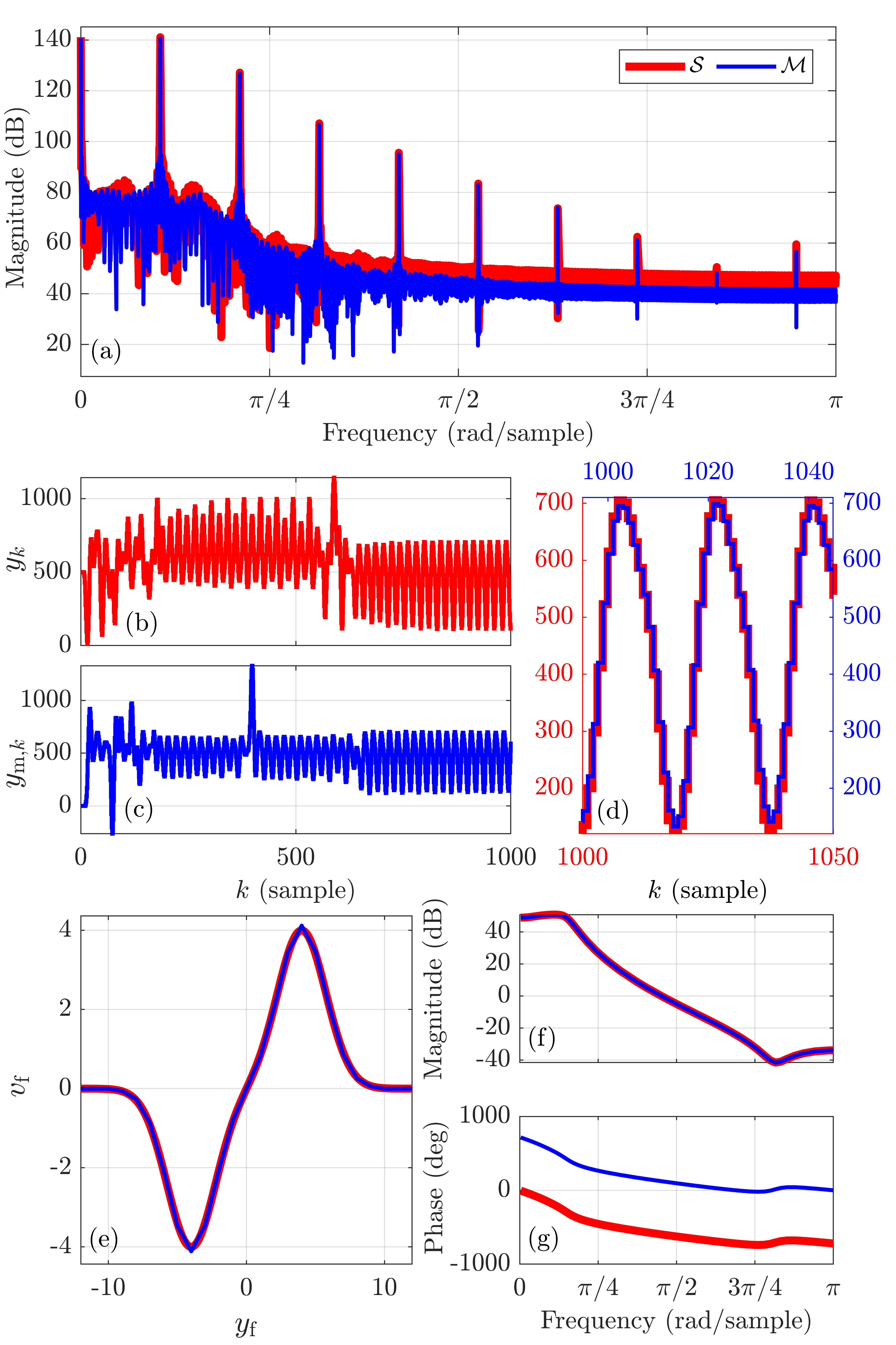
To obtain data for identification, $y_{0},\ldots,y_{6}$ are generated randomly, and, for all $k\geq 0,$ $v_{k}$ is a gaussian random variable with mean 3 and standard deviation $\sqrt{5}.$ For all $k\geq 7,$ $y_{k}$ is generated by simulating ${\mathcal{S}}$ with (68).

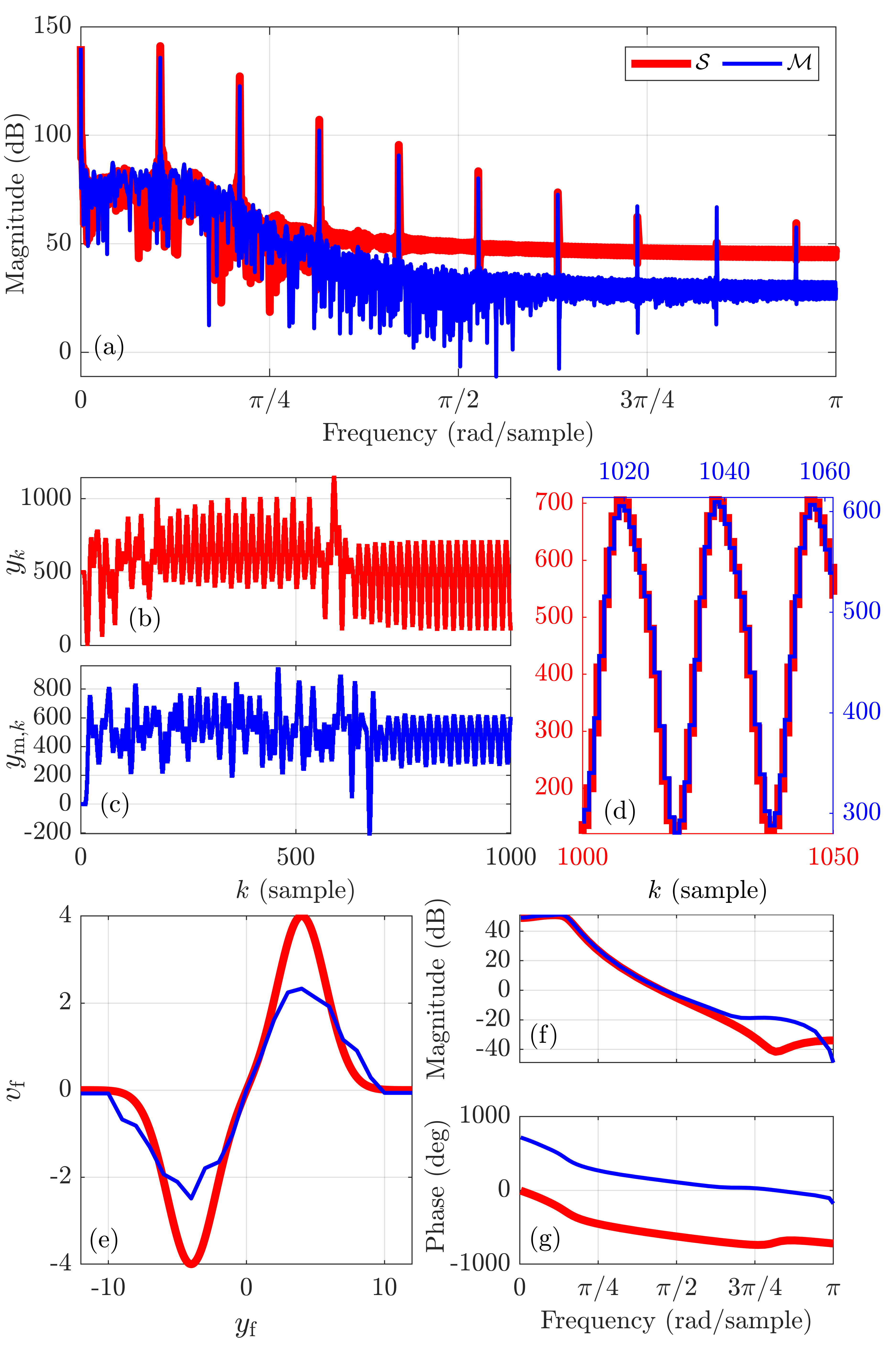
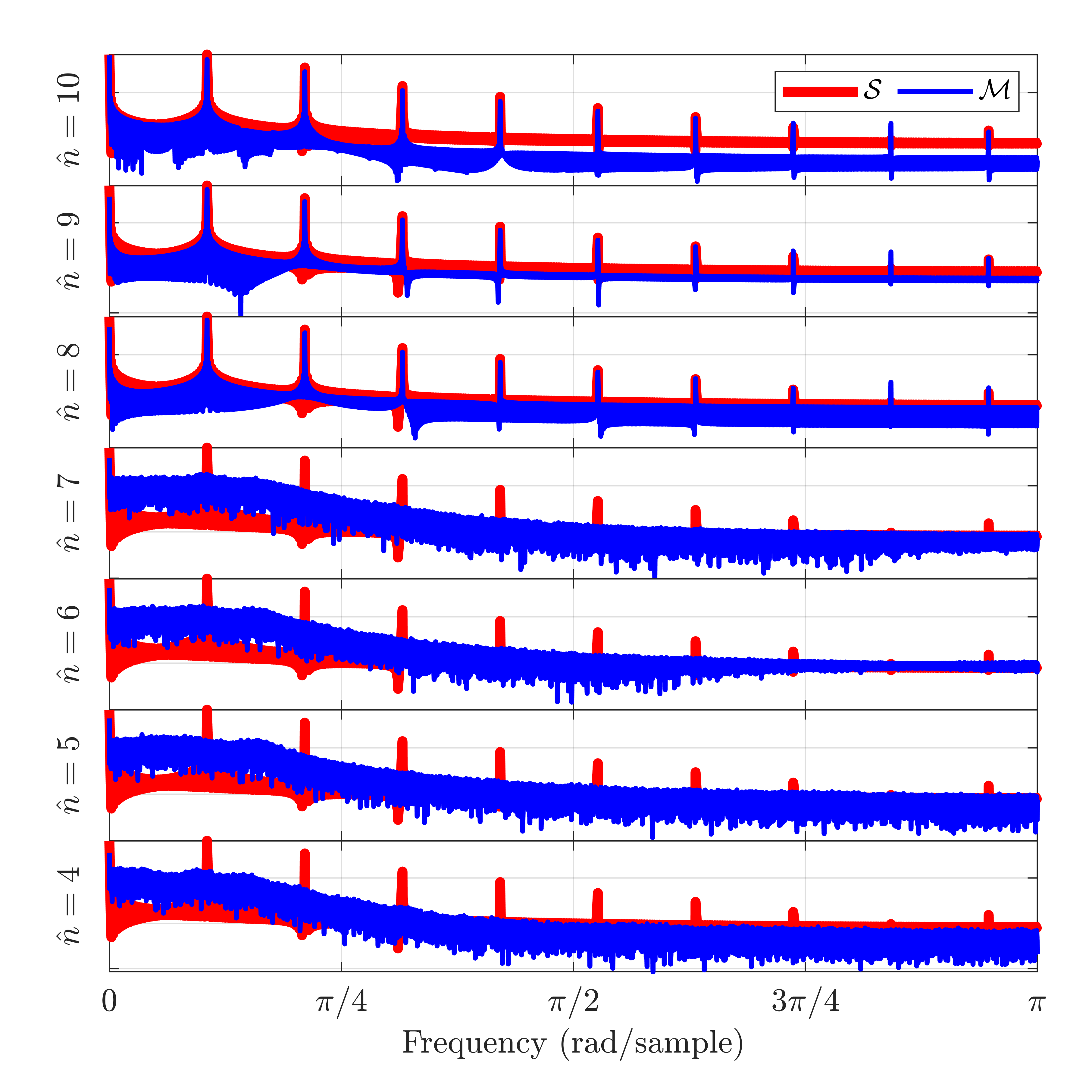
For least-squares identification of the DTTDL/CPL model parameters, we let $\hat{c}={[\begin{array}[]{ccccccc}-10&-9&\cdots&9&10\end{array}]}^{\rm T}$ and $\hat{\beta}=\beta,$ and we apply RLS with $\theta_{0}=0,$ $P_{0}=10^{6}$ and $\lambda=1$ using data in $[100,100000].$ The standard deviation of the sensor noise is chosen to be $\sqrt{2.5},$ which yields a measurement SNR of approximately $55$ dB. To assess the accuracy of the identified model, the input $v_{k}\equiv 2$ is applied to the system ${\mathcal{S}}$ with the initial conditions $y_{k}=500$ for all $k\in[0,6],$ as well as the identified model ${\mathcal{M}}$ with the initial conditions $y_{{\rm m},k}=0$ for all $k\in[0,6].$ The response of the identified model based on noiseless measurements with $\hat{n}=n$ and $\hat{d}=d$ is shown in Figure 11, and the response of the identified model based on noisy measurements with $\hat{n}=10$ and $\hat{d}=d$ is shown in Figure 12. Figure 13 compares the PSD of the output of ${\mathcal{M}}$ for $\hat{n}\in\{4,5,\ldots,9,10\}$ and $\hat{d}=0$ obtained using noisy measurements with the PSD of the output of ${\mathcal{S}}$.

Figure 11: Example 7: Least-squares identification of DTTDL/CPL model parameters using noiseless measurements with $\hat{n}=n$ and $\hat{d}=d.$ (a) compares the PSD of the output of ${\mathcal{M}}$ with the PSD of the output of ${\mathcal{S}}$. (b) shows the output of ${\mathcal{S}}$ with $v_{k}\equiv 2$ and $y_{k}=500$ for all $k\in[0,6].$ (c) shows the output of ${\mathcal{M}}$ with $v_{k}\equiv 2$ and $y_{{\rm m},k}=0$ for all $k\in[0,6].$ (d) shows the output of ${\mathcal{S}}$ on $[1000,1050]$ and the output of ${\mathcal{M}}$ on $[995,1045]$. (e) shows the true and estimated nonlinearities. (f) and (g) show the frequency responses of the linear dynamics of ${\mathcal{S}}$ and ${\mathcal{M}}$.

Figure 12: Example 7: Least-squares identification of DTTDL/CPL model parameters using noisy measurements with $\hat{n}=10$ and $\hat{d}=d.$ (a) compares the PSD of the output of ${\mathcal{M}}$ with the PSD of the output of ${\mathcal{S}}$. (b) shows the output of ${\mathcal{S}}$ with $v_{k}\equiv 2$ and $y_{k}=500$ for all $k\in[0,6].$ (c) shows the output of ${\mathcal{M}}$ with $v_{k}\equiv 2$ and $y_{{\rm m},k}=0$ for all $k\in[0,6].$ (d) shows the output of ${\mathcal{S}}$ on $[1000,1050]$ and the output of ${\mathcal{M}}$ on $[1012,1062]$. (e) shows the true and estimated nonlinearities. (f) and (g) show the frequency responses of the linear dynamics of ${\mathcal{S}}$ and ${\mathcal{M}}$.

Figure 13: Example 7: For $\hat{n}\in\{4,5,\ldots,9,10\}$ and $\hat{d}=0,$ these plots compare the PSD of the output of ${\mathcal{M}}$ identified using noisy measurements with the PSD of the output of ${\mathcal{S}}$.

Example 7: CTTDL system with $C^{\infty},$ monotonic, odd ${\mathcal{N}}$

Let $T_{\rm d}\geq 0$ be the delay time, and let $t\geq 0.$ Furthermore, let $G$ be an $n$th-order strictly proper SISO transfer function with minimal realization $(A,B,C)$ and state $x(t)\in{\mathbb{R}}^{n}.$ Finally, let $G_{\rm f}$ be a SISO washout filter with realization $(A_{{\rm f}},B_{{\rm f}},C_{{\rm f}},D_{{\rm f}})$ and state $x_{\rm f}(t)\in{\mathbb{R}}.$ Then, for all $t\geq T_{\rm d},$ the closed-loop dynamics of the continuous-time, time-delayed Lur’e (CTTDL) model shown in Figure 14 are given by

$$\begin{bmatrix}\dot{x}(t)\\ {\dot{x}}_{{\rm f}}(t)\end{bmatrix}=\begin{bmatrix}A&0\\ 0&A_{{\rm f}}\end{bmatrix}\begin{bmatrix}x(t)\\ x_{{\rm f}}(t)\end{bmatrix}+\begin{bmatrix}0&0\\ B_{{\rm f}}C&0\end{bmatrix}\begin{bmatrix}x(t-T_{{\rm d}})\\ x_{{\rm f}}(t-T_{{\rm d}})\end{bmatrix}+\begin{bmatrix}B\\ 0\end{bmatrix}v_{\rm b}(t),$$ (69)

with output

$$y(t)=\left[\begin{array}[]{cc}C&0\end{array}\right]\left[\begin{array}[]{c}x(t)\\ x_{{\rm f}}(t)\end{array}\right],$$ (73)

the bias-generation mechanism

$$v_{\rm b}(t)=v(t)(\beta+v_{\rm f}(t)),$$ (74)

and signals

$$v_{\rm f}(t) ={\mathcal{N}}(y_{{\rm f}}(t)),$$ (75)

$$y_{{\rm f}}(t) =C_{{\rm f}}x_{{\rm f}}(t)+D_{{\rm f}}y_{{\rm d}}(t),$$ (76)

$$y_{\rm d}(t) =y(t-T_{{\rm d}}).$$ (77)

The resulting bias $\bar{y}$ of the periodic response is thus given by $\bar{y}=v\beta G(0).$ Note that the initialization of (69) depends on $x_{\rm f}(T_{\rm d})$ as well as $x(t)$ for all $t\in[0,T_{\rm d}]$. To compute the solution of the delay differential equations (DDEs) (73)–(77), a Runge-Kutta DDE method is used with an interpolant to approximate the delayed terms, as in (Bellen  Zennaro, 2003, pp. 156–158). In this paper, 4th-order Runge-Kutta is used with a linear interpolant and a fixed time step of 0.001 s.

Figure 14: Continuous-time, time-delayed Lur’e model with constant input $u$ and bias-generation mechanism.

Consider the CTTDL system ${\mathcal{S}}$ with $\beta=50,$ $T_{\rm d}=0.1$ s, $G_{{\rm f}}({\bf p})={\bf p}/(\tau{\bf p}+1)$ with realization $A_{\rm f}=-1/\tau,$ $B_{\rm f}=1,$ $C_{\rm f}=-1/\tau^{2},$ $D_{\rm f}=1/\tau,$ where $\tau=0.001$ s,

$$G({\bf p})=\frac{{\bf p}+2.5}{{\bf p}^{2}+{\bf p}+6.5},$$ (78)

with realization

$$A=\begin{bmatrix}-1&-6.5\\ 1&0\end{bmatrix},\hskip 10.00002ptB=\begin{bmatrix}1\\ 0\end{bmatrix},\hskip 10.00002ptC=\begin{bmatrix}1&2.5\end{bmatrix},$$ (79)

and ${\mathcal{N}}(y_{\rm f})=5\tanh(y_{\rm f}/5).$

To obtain data for identification, let $y_{0}\in{\mathbb{R}}$ and $y(t)=y_{0}$ for all $t\in[0,T_{\rm d}].$ Therefore, for all $t\in[0,T_{\rm d}],$ $\dot{y}(t)=0$, and thus $x(t)=x_{0}$, where

$$x_{0}={\left[\begin{array}[]{c}C\\ CA\end{array}\right]}^{-1}\left[\begin{array}[]{c}y_{0}\\ 0\end{array}\right].$$ (80)

Furthermore, since $y_{\rm d}(T_{\rm d})=y_{0},$ let $x_{\rm f}(T_{\rm d})=\tau y_{0}=0.001y_{0},$ such that $\dot{x}_{{\rm f}}(T_{\rm d})=y_{\rm f}(T_{\rm d})=0.$ For all $t>T_{\rm d},$ $y(t)$ is computed using the DDE method described above, with $y_{0}=0.$ For all $k\geq 0,$ sampled output is $y_{k}=y(kT_{\rm s})$, where $T_{\rm s}=0.1$ s is the sample time.

In the first case, the data are obtained by subjecting ${\mathcal{S}}$ to the constant input $v(t)\equiv 2.5$. For least-squares identification of the DTTDL/CPL model parameters with constant input, we let $\hat{n}=12,$ $\hat{d}=5,$ $\beta_{\rm LS}=5,$ and $\hat{c}={[\begin{array}[]{ccccccc}-6&-5.5&\cdots&5.5&6\end{array}]}^{\rm T},$ and we apply RLS with $\theta_{0}=0,$ $P_{0}={10}^{2}$ and $\lambda=1$ using data in $[100,100000].$ To assess the accuracy of the identified model, $v(t)\equiv 5$ is applied to ${\mathcal{S}}$ with the initial conditions $y(0)=0,$ $x(t)=0$ for all $t\in[0,T_{\rm d}]$ and $x_{\rm f}(T_{\rm d})=0,$ and $v_{k}\equiv 5$ is applied to the identified model ${\mathcal{M}}$ with the initial conditions $y_{{\rm m},k}=0$ for all $k\in[0,17].$ The response of the identified model based on noiseless measurements is shown in Figure 15.

In the second case, the data are obtained by subjecting ${\mathcal{S}}$ to a piecewise-constant input such that, for all $k\geq 0,$ it follows that, for all $t\in[kT_{\rm s},(k+1)T_{\rm s}),$ $v(t)=\omega_{k},$ where $\omega_{k}$ is a gaussian random variable with mean $2.5$ and standard deviation $\sqrt{0.5}.$ For least-squares identification of the DTTDL/CPL model parameters, we let $\hat{n}=12,$ $\hat{d}=4,$ and $\hat{c}={[\begin{array}[]{ccccccc}-12.5&-10&\cdots&10&12.5\end{array}]}^{\rm T},$ and we apply RLS with $\theta_{0}=0,$ $P_{0}={10}^{2}$ and $\lambda=1$ using data in $[100,100000].$ The standard deviation of the sensor noise is chosen to be $\sqrt{2},$ which yields a measurement SNR of approximately 30 dB. To assess the accuracy of the identified model, $v(t)\equiv 5$ is applied to ${\mathcal{S}}$ with the initial conditions $y(0)=0,$ $x(t)=0$ for all $t\in[0,T_{\rm d}]$, and $x_{\rm f}(T_{\rm d})=0.$ The sampled input $v_{k}\equiv 5$ is applied to the identified model ${\mathcal{M}}$ with the initial conditions $y_{{\rm m},k}=0$ for all $k\in[0,16].$ The response of the identified model based on noiseless measurements with $\hat{\beta}=25$ is shown in Figure 16. The response of the identified model based on noisy measurements with $\hat{\beta}=15$ is shown in Figure 17.

Figure 15: Example 7: Least-squares identification of DTTDL/CPL model parameters for constant input measurements using noiseless measurements arising from a constant input $v,$ with $\hat{n}=12,$ $\hat{d}=5,$ and $\beta_{\rm LS}=5.$ (a) compares the PSD of the output of ${\mathcal{M}}$ with the PSD of the output of ${\mathcal{S}}$. (b) shows the sampled output of ${\mathcal{S}}$ with $v(t)\equiv 5$ and $y_{k}=0$ for all $k\in[0,1].$ (c) shows the output of ${\mathcal{M}}$ with $v_{k}\equiv 5$ and $y_{{\rm m},k}=0$ for all $k\in[0,17].$ (d) shows the sampled output of ${\mathcal{S}}$ on $[20000,20100]$ and the output of ${\mathcal{M}}$ on $[19994,20094]$. (e) shows the true and estimated nonlinearities.

Figure 16: Example 7: Least-squares identification of DTTDL/CPL model parameters using noiseless measurements arising from a non-constant input $v,$ with $\hat{n}=12,$ $\hat{d}=4,$ and $\hat{\beta}=25$. (a) compares the PSD of the output of ${\mathcal{M}}$ with the PSD of the output of ${\mathcal{S}}$. (b) shows the sampled output of ${\mathcal{S}}$ with $v(t)\equiv 5$ and $y_{k}=0$ for all $k\in{0,1}.$ (c) shows the output of ${\mathcal{M}}$ with $v_{k}\equiv 5$ and $y_{{\rm m},k}=0$ for all $k\in[0,16].$ (d) shows the sampled output of ${\mathcal{S}}$ on $[2000,2100]$ and the output of ${\mathcal{M}}$ on $[1988,2088]$. (e) shows the true and estimated nonlinearities.

Figure 17: Example 7: Least-squares identification of DTTDL/CPL model parameters using noisy measurements arising from a non-constant input $v,$ with $\hat{n}=12,$ $\hat{d}=4,$ and $\hat{\beta}=15.$ (a) compares the PSD of the output of ${\mathcal{M}}$ with the PSD of the output of ${\mathcal{S}}$. (b) shows the sampled output of ${\mathcal{S}}$ with $v(t)\equiv 5$ and $y_{k}=0$ for all $k\in{0,1}.$ (c) shows the output of ${\mathcal{M}}$ with $v_{k}\equiv 5$ and $y_{{\rm m},k}=0$ for all $k\in[0,16].$ (d) shows the sampled output of ${\mathcal{S}}$ on $[2000,2100]$ and the output of ${\mathcal{M}}$ on $[1989,2089]$. (e) shows the true and estimated nonlinearities.

Example 7: Van der Pol system with bias

Let the ${\mathcal{S}}$ be the continuous-time Van der Pol system

$$\ddot{y}+\mu_{0}(y^{2}-1)\dot{y}+y=0,$$ (81)

where $\mu_{0}$ is a constant parameter. Figure 18 represents ${\mathcal{S}}$ as a Lur’e system.

Figure 18: Block representation of the Van der Pol system, where ${\mathcal{N}}(y,\dot{y})=\mu_{0}(1-y^{2})\dot{y}.$

To obtain data for identification, let $\mu_{0}=1,$ $y(0)=0.1,$ and $\dot{y}(0)=0.$ For all $t>0,$ the Van der Pol system is simulated using ode45, and the output is sampled with sample time $T_{\rm s}=0.1$ s. The integration accuracy of ode45 is set so that approximately 160 integration steps are implemented within each sample interval. A bias $\bar{y}$ is added to all sampled measurements so that, for all $k\geq 0,$ the biased output is $y_{k}=y(kT_{\rm s})+\bar{y}$, where $\bar{y}=10$. Finally, for identification purposes, it is assumed that $v(t)\equiv 1$ is applied to ${\mathcal{S}}.$

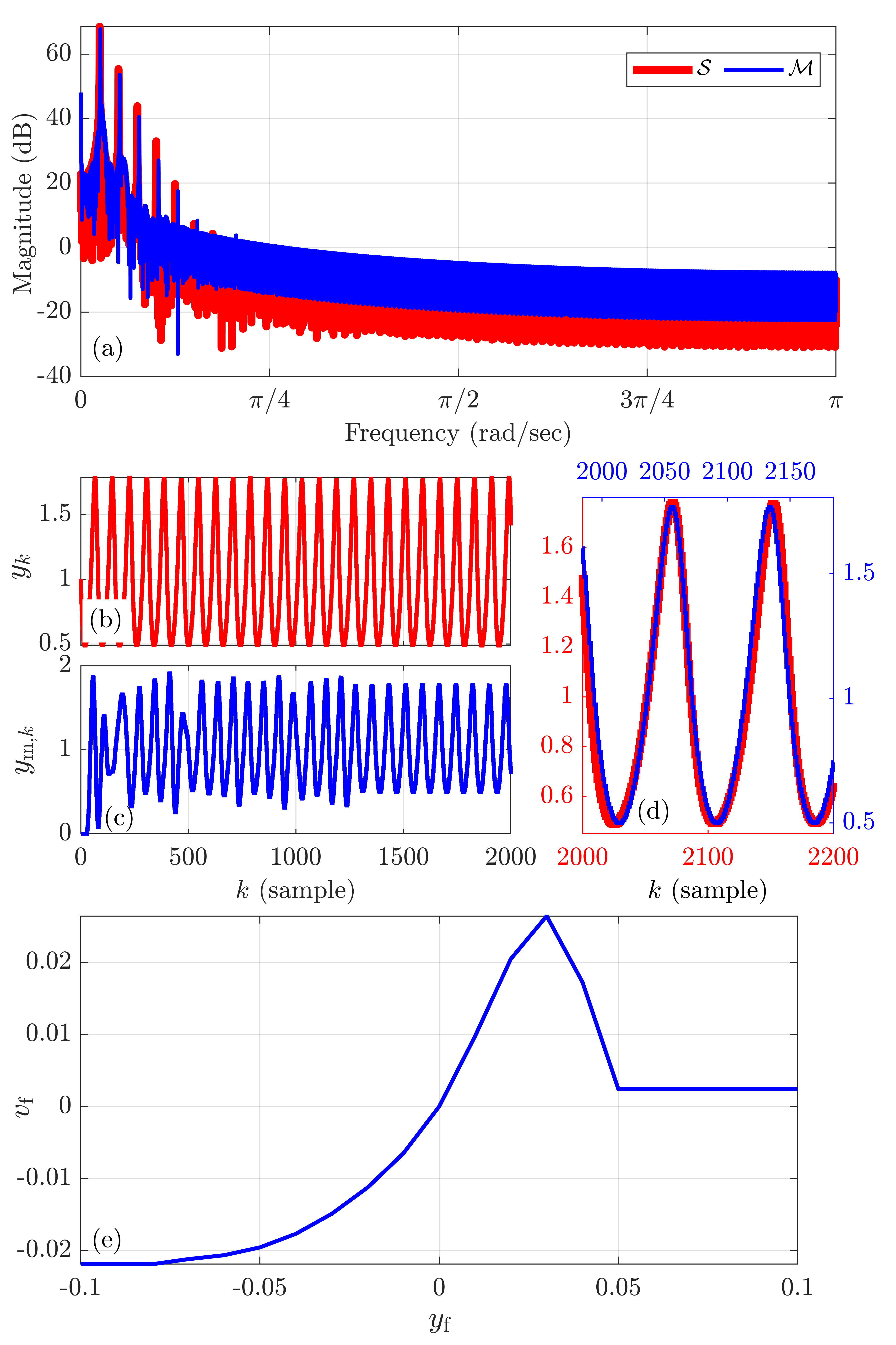
For least-squares identification of the DTTDL/CPL model parameters with constant input, we let $\hat{c}={[\begin{array}[]{ccccc}-0.3&-0.275&\cdots&0.275&0.3\end{array}]}^{\rm T},$ $\hat{n}=12$ and $\hat{d}=19,$ and $\beta_{\rm LS}=-5,$ and we apply RLS with $\theta_{0}=0,$ $P_{0}={10}^{2}$ and $\lambda=1$ using data in $[225,20000].$ To assess the accuracy of the identified model, $v_{k}\equiv 1$ is applied to the identified model ${\mathcal{M}}$ with the initial conditions $y_{{\rm m},k}=0$ for all $k\in[0,31].$ The response of the identified model based on noiseless measurements is shown in Figure 19.

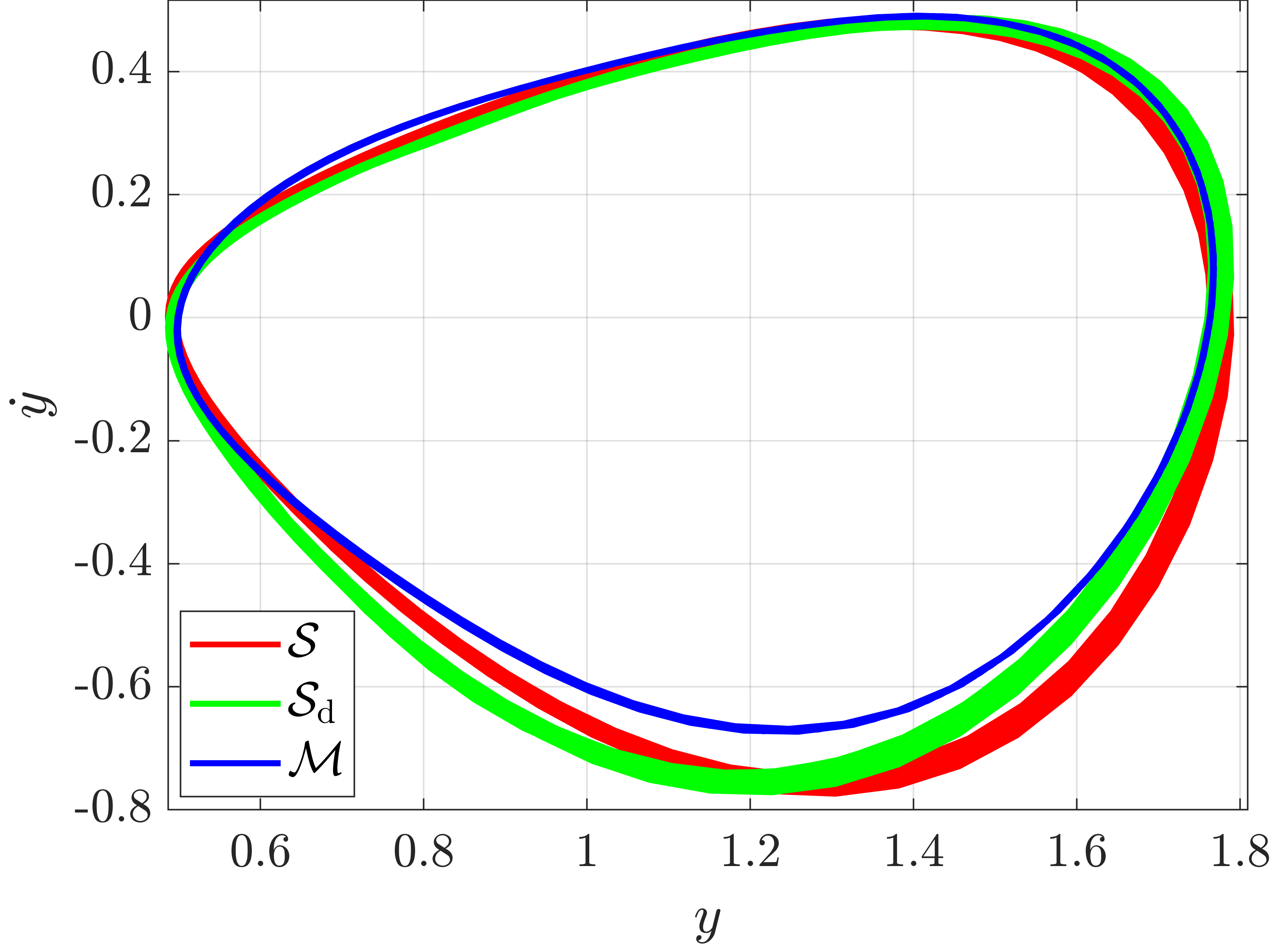
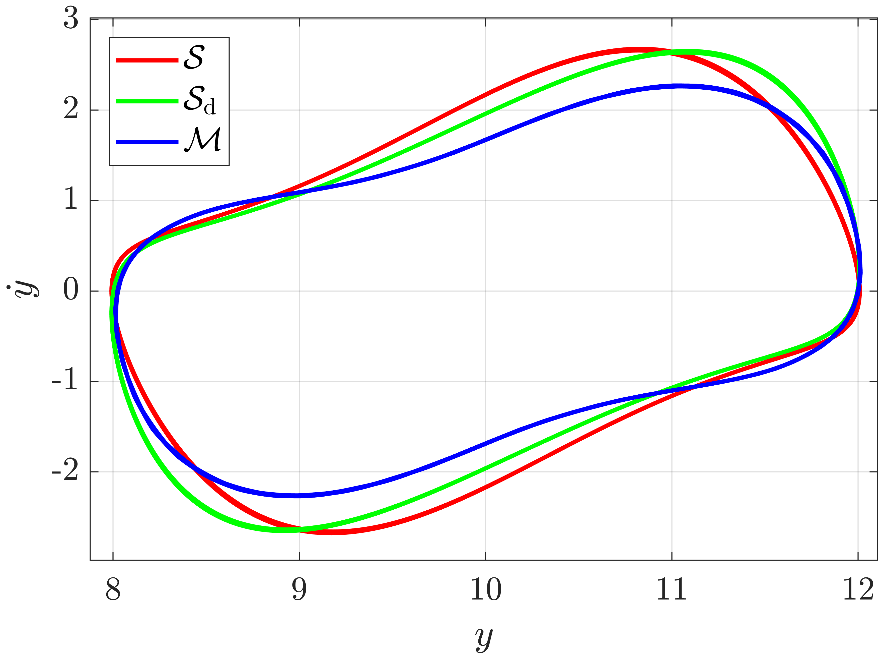
Let ${\mathcal{S}}_{\rm d}$ be the system whose output is the sampled output of ${\mathcal{S}}$ and where the derivative of the sampled output is approximated by $\dot{y}_{k}=\tfrac{y_{k+1}-y_{k-1}}{2T_{\rm s}}.$ Figure 20 compares the phase portraits of the continuous-time system ${\mathcal{S}},$ the discrete-time system ${\mathcal{S}}_{\rm d},$ and the identified model ${\mathcal{M}}$ using $\dot{y}_{k}=\tfrac{y_{k+1}-y_{k-1}}{2T_{\rm s}}$ to approximate the derivative of the output.

Figure 19: Example 7: Least-squares identification of DTTDL/CPL model parameters for constant input measurements using noiseless measurements with $\hat{n}=12,$ $\hat{d}=19,$ and $\beta_{\rm LS}=-5.$ (a) compares the PSD of the output of ${\mathcal{M}}$ with the PSD of the output of ${\mathcal{S}}$. (b) shows the biased sampled output of ${\mathcal{S}}.$ (c) shows the output of the ${\mathcal{M}}$ with $v_{k}\equiv 1$ and $y_{{\rm m},k}=0$ for all $k\leq 31$. (d) shows the sampled output of ${\mathcal{S}}$ on $[555,625]$ and the output of ${\mathcal{M}}$ on $[582,652].$ (e) shows the estimated nonlinear feedback mapping.

Figure 20: Example 7: Phase portraits of the response of the continuous-time Van der Pol system ${\mathcal{S}}$ with $\mu_{0}=1,$ the response of the discrete-time system ${\mathcal{S}}_{\rm d},$ whose output is the sampled output of ${\mathcal{S}},$ and the response of the identified model ${\mathcal{M}}.$ The derivative of the output of ${\mathcal{S}}_{\rm d}$ and ${\mathcal{M}}$ is approximated by using $\dot{y}_{k}=\tfrac{y_{k+1}-y_{k-1}}{2T_{\rm s}}.$

Example 7: Predator-prey Lotka-Volterra system

Let the ${\mathcal{S}}$ be the continuous-time predator-prey Lotka-Volterra system

$$\dot{y} =\zeta y-\varrho xy,$$ (82)

$$\dot{x} =-\xi x+\varphi xy,$$ (83)

where $\zeta,\varrho,\xi,\varphi$ are constant parameters.

To obtain data for identification, let $\zeta=2/3,$ $\varrho=4/3,$ $\xi=1,$ $\varphi=1,$ and $y(0)=x(0)=1.$ For all $t>0,$ the Lotka-Volterra system is simulated using ode45, and the output is sampled with sample time $T_{\rm s}=0.1$ s. The integration accuracy of ode45 is set so that approximately 160 integration steps are implemented within each sample interval. Finally, for identification purposes, it is assumed that $v(t)\equiv 1$ is applied to ${\mathcal{S}}.$

For least-squares identification of the DTTDL/CPL model parameters with constant input, we let $\hat{c}={[\begin{array}[]{ccccc}-0.08&-0.07&\cdots&0.05&0.06\end{array}]}^{\rm T},$ $\hat{n}=12$, $\hat{d}=13,$ and $\beta_{\rm LS}=-5,$ and we apply RLS with $\theta_{0}=0,$ $P_{0}={10}^{2},$ and $\lambda=1$ using data in $[500,10000].$ To assess the accuracy of the identified model, $v_{k}\equiv 1$ is applied to the identified model ${\mathcal{M}}$ with the initial conditions $y_{{\rm m},k}=0$ for all $k\in[0,25].$ The response of the identified model based on noiseless measurements is shown in Figure 21.

Let ${\mathcal{S}}_{\rm d}$ be the system whose output is the sampled output of ${\mathcal{S}}$ and where the derivative of the sampled output is approximated by $\dot{y}_{k}=\tfrac{y_{k+1}-y_{k-1}}{2T_{\rm s}}.$ Figure 22 compares the phase portraits of the continuous-time system ${\mathcal{S}},$ the discrete-time system ${\mathcal{S}}_{\rm d},$ and the identified model ${\mathcal{M}}$ using $\dot{y}_{k}=\tfrac{y_{k+1}-y_{k-1}}{2T_{\rm s}}$ to approximate the derivative of the output.

Figure 21: Example 7: Least-squares identification of DTTDL/CPL model parameters for constant input measurements using noiseless measurements with $\hat{n}=12,$ $\hat{d}=13,$ and $\beta_{\rm LS}=-5.$ (a) compares the PSD of the output of ${\mathcal{M}}$ with the PSD of the output of ${\mathcal{S}}$. (b) shows the biased sampled output of ${\mathcal{S}}.$ (c) shows the output of the ${\mathcal{M}}$ with $v_{k}\equiv 1$ and $y_{{\rm m},k}=0$ for all $k\leq 25$. (d) shows the sampled output of ${\mathcal{S}}$ on $[2000,2200]$ and the output of ${\mathcal{M}}$ on $[1985,2185].$ (e) shows the estimated nonlinear feedback mapping.

Figure 22: Example 7: Phase portraits of the response of the continuous-time Lotka-Volterra system ${\mathcal{S}}$ with $\zeta=2/3,\varrho=4/3,\xi=1,\varphi=1,$ and $y(0)=x(0)=1,$ the response of the discrete-time system ${\mathcal{S}}_{\rm d},$ whose output is the sampled output of ${\mathcal{S}},$ and the response of the identified model ${\mathcal{M}}.$ The derivative of the output of ${\mathcal{S}}_{\rm d}$ and ${\mathcal{M}}$ is approximated by using $\dot{y}_{k}=\tfrac{y_{k+1}-y_{k-1}}{2T_{\rm s}}.$

8 Conclusions and future work

This paper developed a technique for identification of self-excited systems (SES) based on a discrete-time, time-delayed Lur’e (DTTDL) model. The nonlinear feedback mapping was chosen to be a continuous, piecewise-linear (CPL) function characterized by its slope in each interval of a user-chosen partition of the real line. By minimizing a bound on a nonquadratic cost function, linear least-squares techniques were used for parameter estimation within DTTDL/CPL.

Numerical examples included both discrete-time and continuous-time systems with sampled data. Of particular interest was the ability of the DTTDL model to reproduce the limit-cycle response of the Van der Pol oscillator and the Lotka-Volterra model. Although neither of these systems have the structure of a DTTDL model, the system identification technique was able to approximately reproduce the phase-plane dynamics of both systems.

Future research will focus on efficient techniques for determining the user-chosen partition of the real line needed to parameterize the static nonlinear feedback mapping. Finally, the numerical results motivate a fundamental research question, namely, to what extent can DTTDL/CPL models approximate the response of an arbitrary SES system.

9 Acknowledgments

This research was supported by NSF grant CMMI 1634709, “A Diagnostic Modeling Methodology for Dual Retrospective Cost Adaptive Control of Complex Systems.”